ON A FUNCTIONAL-DIFFERENTIAL EQUATION ARISING FROM … · ON A FUNCTIONAL-DIFFERENTIAL EQUATION ARISING FROM ... The model is related to the macroscopic tra c model rst suggested

ON A FUNCTIONAL-DIFFERENTIAL EQUATION ARISING FROMA TRAFFIC FLOW MODEL∗

REINHARD ILLNER AND GEOFFREY MCGREGOR†

Abstract. We provide a derivation in the context of a traffic flow model, and both analyticaland numerical studies of the functional-differential equation

(z(s) + α)2z′(s) = β(z(s+ z(s)) − z(s)).

Here, α and β are positive parameters, and we are in particular investigating the existence andproperties of non-constant “traveling-wave” type solutions.

Key words. Kinetic and macroscopic traffic flow models, traveling waves, functional-differentialequations

AMS subject classifications. 34K99,35L65,82D99

1. Introduction. The subject of interest of this article is the functional-differentialequation

(z(s) + α)2z′(s) = β(z(s+ z(s))− z(s))(1.1)

This equation arises in a search for traveling wave solutions of a macroscopic trafficflow model (first introduced in [14]) which takes the inherent non-locality of trafficseriously. We will refer to (1.1) as “jam” equation because it emerges from a search forbraking waves. The model is related to the macroscopic traffic model first suggestedby Aw and Rascle [1], and independently by Zhang [31]. Our paper is, in particular,a continuation of [15], where we presented mathematical and numerical analysis ofthe model. The emphasis in [15] was on a careful model refinement and on studies ofits predictions under certain traffic scenarios, such as local speed limits, density per-turbations or speed reductions. In particular, we investigated (numerically) whethertraveling wave approximations would properly apply in suitable road intervals. Theresults in [15] gave an affirmative answer to this query, and they also showed thatsimplifications of the model in which the non-locality is removed by Taylor approxi-mation to second order, while simpler and qualitatively satisfying, give significantlydifferent results from a quantitative point of view.

In [15] no effort was made to analytically or numerically solve (1.1); rather, so-lutions of the full model of conservation type equations were checked to satisfy thetraveling wave version (essentially (1.1)) in appropriate subdomains of the road. Astudy of (1.1) was deferred to the future, i.e., to this present work.

Functional-differential equations have been studied for centuries, but their the-ory suffers, to some extent, from a very limited toolbox. Existence and uniquenessquestions can be much more subtle than for ordinary or partial differential equa-tions. Analytic expansions of Cauchy-Kowalewskaya type are routinely applied, butthey provide typically only locally defined solutions. The monograph [3] provides theframework and many examples for this approach. However, we state from the outsetthat our efforts to apply this methodology to (1.1) were not satisfactory.

Our work begins, in Section 2, with a brief review of the derivations given inthe earlier references [14, 15]. This is also the place where crucial traffic parameters

∗Supported by grants from the Natural Science and Research Council of Canada.†Department of Mathematics and Statistics, University of Victoria, PO BOX 3060 STN CSC,

Victoria, BC V8W 3R4, CANADA

1

2 R. Illner and G. McGregor

such as H (minimal safety distance), T (look-ahead time) and τ (individual reactiontime) are introduced. We then focus on the functional-differential equations arisingfrom a traveling wave ansatz in braking scenarios (similar considerations apply toacceleration cases, but will here not be discussed; the derivation and analysis of thesescenarios requires model refinements and will be done elsewhere [25]). A preliminarydiscussion is provided in Section 8.

The crucial difficulty in our traveling wave equations is the non-locality arisingfrom realistic driver behaviour. This non-locality can be removed via a Taylor expan-sion and crude truncation, as already discussed in [14, 15]. The truncated (“localized”)equations admit beautiful traveling waves; however, as seen from the numerical ex-periments in [15], the truncation will in general cause a significant error, because thedisplacement H + Tu(x, t), “removed” via Taylor expansion, is in general not small,and hence the truncation of the expansion will lead to errors. For that reason theinclusion of the full non-locality is not just a matter of theoretical interest; rather, itappears that it is essential for a detailed resolution of the velocity profiles in brakingwaves.

We review the derivation of the macroscopic model in Section 2, and the travelingwave ansatz and its localized version in Section 3.

In Section 4 we simplify the full (non-localized) traveling wave equation via affinetransformations. The end result is equation (1.1) for z = z(s) (where s is the variables = x+ V t and z is a rescaled speed variable)

(z(s) + α)2z′(s) = β(z(s+ z(s))− z(s)).

There remain only two parameters α, β, combinations of the original model parame-ters. The main question of interest is for what values of α > 0, β > 0 (1.1) will admitnon-trivial (i.e., non-constant) solutions. This is a question not just of some practicalinterest for traffic flow studies. We hope to convince the reader that (1.1) is an objectof pure mathematical interest in itself, and we follow a variety of avenues to answerthe main question. While we have no complete solution, we will show evidence thatnon-trivial and stable traveling waves solving (1.1) will exist or fail to exist, dependingon the values of the parameters. A remarkable practical aspect of our study is thatit provides quite realistic upper and lower bounds for the traveling wave speeds.

In Section 5 we present two examples related to (1.1): First, a simpler linearfunctional-differential equation with a constant non-locality; for this example it iseasy to construct explicit solutions, and they allow an interpretation in terms ofelementary geometric operations. Secondly, we try a “Mott-Smith”- approximation[4] in the sense that we insert an ansatz z(s) = A+B tanh(−σs) into the equation. Itturns out that the equation is not satisfied (no surprise there), but if we force equalitybetween the two sides by allowing β = β(s) to be dependent on s, then the resultingfunctions β are asymptotically constant for large |s|; moreover, an exploration whichwe defer until Appendix 1 shows that there are many parameter choices (A,B, σ, α)for which β(−∞) = β(+∞). The point of these examples is to provide evidence thatthere actually are equations closely related to (1.1) with non-trivial solutions of thedesired class.

Section 6 returns to the real equation (1.1). In this section we describe a numer-ical approximation procedure to compute (approximate) solutions. The method isbased on a dynamical systems idea and suggests rapid convergence for a select set ofparameters. It is not to be expected that the traveling wave solutions we are lookingfor will exist for all (or even most) choices of parameters. In Appendix 2 we present

Functional-Differential Equation in Traffic Flow 3

a situation where the dynamical systems approach fails to converge. There may beno solution of (1.1) for the parameters and boundary values used there.

In Section 7 we describe an operator approach to the solvability question. This,the most abstract of our sections, is heavily motivated by geometric interpretation,and we introduce and discuss two operators T1, T2 acting on wave profiles such thata solution z of (1.1) of the desired type will satisfy T1z = T2z, a fixed point equation.We collect a number of intriguing properties of these operators, suggesting that a fixedpoint argument is a viable approach to the existence question, but we need some apriori assumptions to complete this argument. Whether these assumptions can beverified remains an avenue for future work.

While our problem arose in traffic flows models, it is treated here as an abstractmathematical challenge. Its practical relevance for traffic applications will dependon the degree to which the underlying model is accepted as realistic, and, if this isthe case, whether high resolution of speed profiles can be exploited to improve trafficcontrol. We discuss these matters in Section 8.

There is extensive mathematical literature on traffic flow models (see [15] and thereferences therein). Traffic models may roughly be classified as “microscopic” (keepingtrack of each car in a deterministic way, see for example [6, 7, 12, 13, 22, 24]), ofstochastic type (there is much variation here; see [2, 28, 29]), or variations includingboth features, such as cellular automata [12, 26, 27]. The model which leads toEquation (1.1) is of macroscopic type, and earlier versions of macroscopic models andtheir analysis may be found in [1, 8, 9, 10, 11, 17, 18, 23, 30]. Kinetic models are apossible bridge between microscopic/ stochastic and macroscopic models, as discussedin [20, 5, 21].

An inherent problem in all traffic modelling is the complexity of drivers’ reactions,which poses a serious obstacle to accuracy at all levels, and is a persistent sourceof criticism of all models. While validation of models from both a theoretical andpractical point of view remains elusive for this “human” factor, traffic models oftenlead to intriguing mathematical challenges, like the functional-differential equationwhich is the object of our study.

2. The macroscopic model. Reference [15] introduced the following kineticmodel for traffic on a single-lane (or homogenized over several lanes) highway:

∂tf + v∂xf + ∂v(B(ρ, v − uX)f) = 0(2.1)

where f = f(x, v, t) is a kinetic car density such that fdxdv will be the statisticallyexpected car number in the space and speed domain [x, x + dx] × [v, v + dv] , and ρand u are the macroscopic density and speed, related to f via

ρ =

∫ ∞0

fdv, ρu =

∫ ∞0

vfdv.

The shorthand uX in (2.1) stands for uX = u(x + H + Tv, t − τ). Here, H > 0is a constant safety distance (think of two car lengths) which drivers keep at lowspeeds, measured from car front to car front. T is a characteristic “look-ahead” timeused to keep an appropriate distance to the lead car, and τ is the individual reactiontime. The term B(. . .) in (2.1) denotes the braking or acceleration force applied by areference driver at position x and moving with speed v at time t.

Equation (2.1) must be interpreted in a statistical sense (a comment which appliesto all kinetic models, but is often ignored for models involving microscopic particles


such as atoms or electrons), and although we have incorporated a non-locality, themodel is likely to be overly simplistic from a practical point of view: we assumethat the forces depend only on the local density (ρ) and on the relative speed ofthe reference driver with respect to the delay-observed average speed uX at positionx+H +Tv. While this makes sense, reality certainly requires random fluctuations inthese forces, which are not included in (2.1). In addition, one could consider equationslike (2.1) for many different lanes and include lane-changing terms on the right-handsides. Some of this was done in [20] and subsequent papers [16]. Here, we aim atstructural problems emerging from the non-locality, and we therefore keep thingssimple.

A reasonable ansatz for the braking or acceleration force is

B(ρ, v − uX) =

{−g1(ρ)(v − uX) if v − uX > 0−g2(ρ)(v − uX) if v − uX < 0

(2.2)

and simple “reasonable” choices for g1, g2 are

g1(ρ) = c1ρ, g2(ρ) = c2(ρmax − ρ)

(the maximal density is ρmax = 1/H, where H is the minimal safety distance betweenthe fronts of two vehicles; in standing traffic we may have real bumper-to-bumpertraffic, and then ρmax = 1/L, where L is the average length of a car. One may guessthat H ≈ 2L). It must be stated here that (2.2) is overly simplistic, but as this is nota paper on the details of traffic modelling, we will not pursue the delicacies of driverbehaviour. Some of these matters are discussed in [15], and in [22].

How does one go from a kinetic model to a macroscopic model? One method,used in [19], is to set up and study moment equations. Typically a closure procedureis needed to obtain a finite (closed) set of equations, and this closure will involveassumptions on the system at hand. There is a more direct (if rough) approach:in moderate to high traffic densities (which in reality are the relevant densities) oneexpects (based on observations) only small statistical fluctuations. Traffic is oftendescribed as “synchronized”, meaning that all vehicles at time t and near position xwill move at approximately the same speed. This motivates the ansatz f(x, v, t) =ρ(x, t)δ(v − u(x, t)) in (2.1), and we have the following general result.

Theorem 2.1. Assume that ρ = ρ(x, t) and u = u(x, t) are of class C1. Thenthe distribution ρ(x, t)δ(v − u(x, t)) is a weak solution of (2.1) if and only if ρ and usatisfy the system of equations

ρt + (ρu)x = 0(2.3)

ut + uux −B(ρ, u− uX) = 0.(2.4)

Remark 1. The first equation is just the continuity equation, while the secondequation is the equation for the speed. In equation (2.4) the meaning of the superscript()X has changed: Now, uX(x, t) = u(x+H+Tu(x, t), t−τ). Notice how the dependentvariable u here appears inside its own argument.

Proof. The proof we present is a more transparent version of the proof given in[15]. The key idea is to exploit the different status of the variables x, t and v. For


simplicity, assume that the (kinetic) density f vanishes rapidly as x → ±∞, and asv → 0 or v → ∞ (this assumption certainly holds for the ansatz ρ(x, t)δ(v − u(x, t))while u > 0.) Then f is a weak solution of the kinetic model if for every test functionφ(x, v, t), compactly supported in x, t and arbitrary but bounded in v, we have∫ ∫ ∫

φtf + φxvf + φvB(ρ, v − uX)f dx dv dt = 0.(2.5)

We substitute in (2.5) a test function of the form φ(x, v, t) = ϕ(x, t)h(v). Set ψ(x, t) :=φ(x, u(x, t), t) = ϕ(x, t)h(u(x, t)), then

ψt = φt + φvut= ϕth+ ϕh′ut

ψx = φx + φvux= ϕxh+ ϕh′ux.

Rewrite φt = ψt − ∂vφut and φx = ψx − ∂vφux and substitute in (2.5), to find∫ ∫ ∫[ψtf + ψxvf − ϕh′(v)utf − ϕh′(v)uxvf + ϕh′(v)B(. . .)f ] dv dx dt = 0,

and for f = ρδ(v − u) this becomes∫ ∫[ψtρ+ ψxρu]−

∫ ∫ψh′(u)

h(u)ρ[ut + uux −B(ρ, u− uX)] = 0,

provided we assume that h is bounded away from zero. We may then consider ψ asan arbitrary test function and observe that the last integral contains the extra degreeof freedom h′

h . It follows that both integrals must vanish identically, and our resultfollows from this.

Remark 2. It is a simple and natural idea to remove the nonlinearity in (2.4) byusing a (formal) Taylor expansion. In a braking scenario, if we take B(ρ, u− uX) =−g1(ρ)(u − uX) and expand to first order u − uX ≈ −(H + Tu)ux, we obtain thesimpler equation

ut + uux − g1(ρ)(H + Tu)ux = 0.(2.6)

In combination with the continuity equation, (2.6) is a generalization of the Aw-Rasclemodel [1], for which the speed transfer equation is usually written as

ut + uux − ρ∂p

∂ρux = 0.

Here,

pρ =∂p

∂ρ(ρ, u) =

g1(ρ)

ρ(H + Tu).

This generalizes the Aw-Rascle model inasmuch as p depends on both ρ and u, whileonly a dependence on ρ was assumed in [1]. A similar equation applies to the ac-celeration scenario, and in combination these two equations form a traffic model ofHamilton-Jacobi type. One can easily consider models in which the second order termsin the Taylor expansion is retained, as already done in [14, 15]. The resulting modelscan be considered as Hamilton-Jacobi type models with diffusive corrections.


3. On Traveling Waves. The models introduced above readily offer themselvesto numerical analysis, in particular because the non-locality arises in a term with atime delay (i.e., the velocity profile needed in the calculation will have been computedin previous steps). Extra care, and modelling refinements, are needed in transitiondomains between braking and acceleration; as already mentioned, we plan to addressthese issues in future work [25].

Interesting quandaries arise in searching for traveling wave solutions, and thisis the main theme addressed here. A traveling wave solution will be of the formρ = ρ(s), u = u(s) where s = x+V t and V is the speed of the traveling wave. We willimplicitly always assume V > 0, so with s = x+ V t waves will be moving backwardsin traffic. It is useful to note at this point that observations suggest realistic wavespeeds V ≈ 20 km/hr, or about 5.5 meters per second. We will pause intermittentlyin our progress to compare results with this benchmark.

With the traveling wave ansatz the continuity equation becomes dds [ρ(u+V )] = 0,

which gives

ρ(s) =c0V

u+ V,

with an integration constant c0 > 0 (in [14] we set c0 = ρmax, motivated by theobservation that in standing traffic (u = 0) we expect ρ = ρmax. However, othervalues of c0 are perfectly consistent with the continuity equation).

Substituting this ρ into (2.4) and setting g1(ρ) = c1ρ, we find the equation for atraveling braking wave,

(u(s) + V )2u′(s) = c0c1V [u(s+ (H − τV ) + Tu(s))− u(s)].(3.1)

This is a functional-differential equation. Observe how u(s) shows up inside the argu-ment of u itself. Equation (3.1) contains no fewer than 6 parameters (H,T, τ, c0, c1, V ).We will shortly see that all but two parameters can be eliminated via affine transfor-mations. Equation (3.1) suggests to restrict our discussion to V < H/τ, so that forany u(s) > 0 we will have Tu(s) +H − τV > 0, a “causality” constraint.

3.1. Removing the nonlocality by Taylor expansion. This simple idea wasalready followed in [14, 15], but we include it here for completeness. It also providesfurther insight on the relationships between parameters. Here, it is implicitly assumedthat u has sufficiently many derivatives.

A Taylor expansion to second order gives

u(s+(H−τV )+Tu(s))−u(s) = (H−τV +Tu(s))u′(s)+1

2(H−τV +Tu(s))2u′′(s)+. . .

After neglecting terms of third and higher order and substituting into (3.1) one finds

u′′ = 2(u+ V )2 − c0c1V (H − τV + Tu)

c0c1V (H − τV + Tu)2u′.(3.2)

This equation is easily studied in phase space u, u′, because it follows from (3.2) that

du′

du= 2

(u+ V )2 − c0c1V (H − τV + Tu)

c0c1V (H − τV + Tu)2.(3.3)


Every point (u > 0, u′ = 0) is a (trivial) solution of (3.2). If the condition

V <c0c1H

1 + c0c1τ

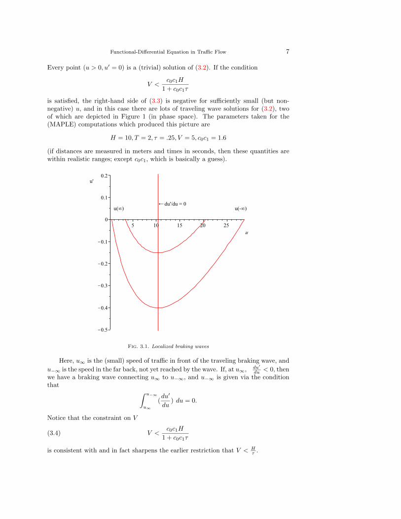
is satisfied, the right-hand side of (3.3) is negative for sufficiently small (but non-negative) u, and in this case there are lots of traveling wave solutions for (3.2), twoof which are depicted in Figure 1 (in phase space). The parameters taken for the(MAPLE) computations which produced this picture are

H = 10, T = 2, τ = .25, V = 5, c0c1 = 1.6

(if distances are measured in meters and times in seconds, then these quantities arewithin realistic ranges; except c0c1, which is basically a guess).

Fig. 3.1. Localized braking waves

Here, u∞ is the (small) speed of traffic in front of the traveling braking wave, and

u−∞ is the speed in the far back, not yet reached by the wave. If, at u∞,du′

du < 0, thenwe have a braking wave connecting u∞ to u−∞, and u−∞ is given via the conditionthat ∫ u−∞

u∞

(du′

du) du = 0.

Notice that the constraint on V

V <c0c1H

1 + c0c1τ(3.4)

is consistent with and in fact sharpens the earlier restriction that V < Hτ .


A similar analysis applies to acceleration waves with the corresponding equationfor acceleration scenarios. They fill the upper half of the phase portrait depicted inFigure 1. Examples for this (with τ = 0) are given in [14].

4. The “Jam” equation. We return to the equation displaying the full non-locality,

(u(s) + V )2u′(s) = c0c1V [u(s+ (H − τV ) + Tu(s))− u(s)].(4.1)

A simple and natural idea is to try and reduce the number of parameters by affinetransformations in both independent and dependent variables. It is straightforwardto do that; elementary calculations show that if we set

δ :=1

T(H − τV ), z(s) := T (u(s) + δ)

then z = z(s) satisfies the simpler equation

(z(s) + α)2z′(s) = β(z(s+ z(s))− z(s)).(4.2)

with

α = T (V − δ) and β = c0c1V T2.(4.3)

This is the “jam” equation already given in (1.1). It contains only the two parametersα, β and the (simpler) non-locality z(s+ z(s)).

Our implicit assumption u > 0 translates into z > Tδ = H − τV. If we add the(somewhat arbitrary) assumption that α > 0 then it follows that δ < V, which meansH < V (T + τ). While this final condition on V is less motivated than the earlier ones,it is instructive to write the sequence of constraints imposed so far:

H

T + τ< V <

c0c1H

1 + c0c1τ<H

τ,

where the last estimate is obvious; note that the final upper bound depends only andH and τ. In reality, one has (approximately) τ ≈ 1 sec, H ≈ 8 m, T ≈ 3 sec. Insertingin the inequalities above one gets

H

T + τ≈ 2 m/sec < V < 8 m/sec ≈ H

τ,

which translates into V s between 8 and 30 km/h — very much the observed range(5.5 m/sec).

We are looking for a special class of solutions of (4.2), namely, braking waves. Abraking wave is a solution of (4.2) such that ∀s z′(s) < 0, and such that z(−∞) =a > b = z(∞) > δ > 0. Here, a, b are (shifted and rescaled) speeds at ±∞. If a = b,the constant a is a trivial solution of (4.2) and it is immediate that every constantsolves (4.2). We will implicitly assume that (4.2) is complemented with boundaryconditions at infinity such that a > b. Two remarks are in order.


• Translation invariance: If z = z(s) is a solution of the jam equation, then sois Ss0z(s) := z(s− s0).

• Consistency: While z(s) takes nonnegative values and is decreasing, we havez(s+ z(s))− z(s) ≤ 0, consistent with z′(s) ≤ 0. However, it is in general nottrue that s → z(s + z(s)) will decrease if z′(s) < 0. See Section 7 for moredetails.

The hardest question we face is whether non-trivial braking waves as solutions of(4.2) actually exist. As the problem appears rather inaccessible to standard analyticaltools, we now provide some related illuminating examples, and numerical evidence.We revisit the existence question in Section 7.

5. Related examples.

5.1. A linear example. Consider the much simpler linear example

z′ = β(z(s+ z0)− z(s)),

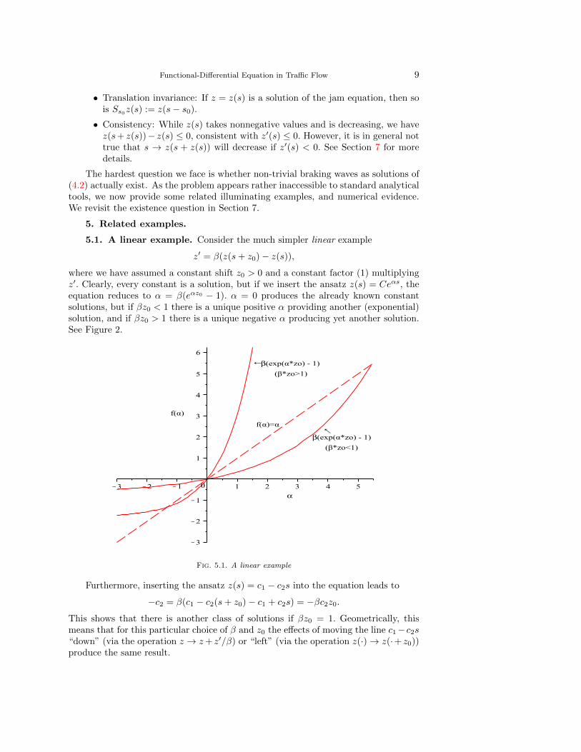
where we have assumed a constant shift z0 > 0 and a constant factor (1) multiplyingz′. Clearly, every constant is a solution, but if we insert the ansatz z(s) = Ceαs, theequation reduces to α = β(eαz0 − 1). α = 0 produces the already known constantsolutions, but if βz0 < 1 there is a unique positive α providing another (exponential)solution, and if βz0 > 1 there is a unique negative α producing yet another solution.See Figure 2.

Fig. 5.1. A linear example

Furthermore, inserting the ansatz z(s) = c1 − c2s into the equation leads to

−c2 = β(c1 − c2(s+ z0)− c1 + c2s) = −βc2z0.

This shows that there is another class of solutions if βz0 = 1. Geometrically, thismeans that for this particular choice of β and z0 the effects of moving the line c1−c2s“down” (via the operation z → z+ z′/β) or “left” (via the operation z(·)→ z(·+ z0))produce the same result.


5.2. The tanh− (or “Mott-Smith”) approximation. One of the fundamen-tal ideas of the “Mott-Smith” approximation (see, for example, [4] and the referencestherein) in fluid dynamics is to fit a hyperbolic tangent profile to a shock wave; therelevant dependent variables there are density, macroscopic flow speed, pressure andtemperature. It is tempting to do the same here, where the traveling wave ansatz hasalready reduced the complexity to one dependent variable, z(s).

Remarkably, if we consider the function z(s) := A + B tanh(−σs), (it is a littlesloppy to use the same same symbol z for this function, but we will do it anyway),and use the identities

d

dstanh(s) = 1− tanh2(s)

tanh(x+ y) =tanh(x) + tanh(y)

1 + tanh(x) tanh(y)

we find that this z satisfies an equation

(z(s) + α)2z′(s) = β(s)(z(s+ z(s))− z(s)),(5.1)

where β(s) =

−σ(α+A+B tanh(−σs))2(1 + tanh(−σs) tanh(−σ(A+B tanh(−σs))))tanh(−σ(A+B tanh(−σs)))

.(5.2)

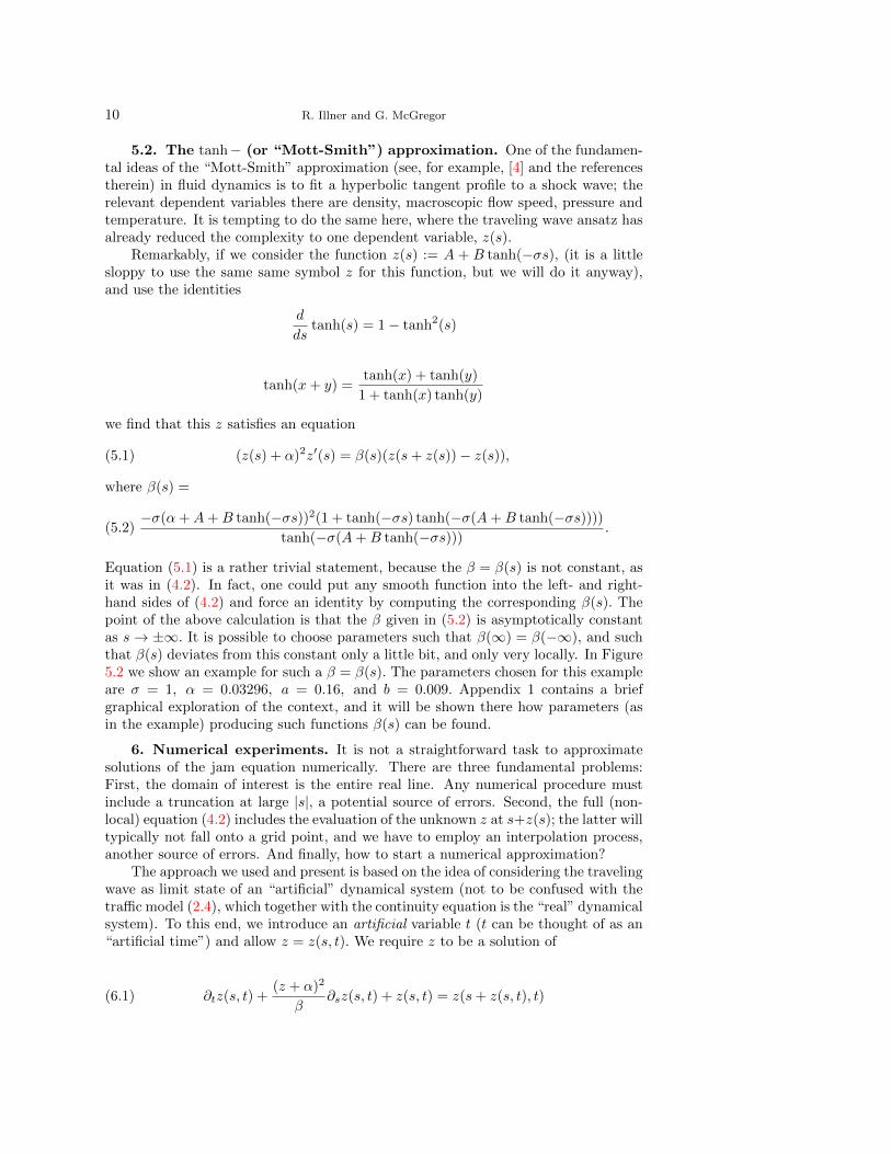
Equation (5.1) is a rather trivial statement, because the β = β(s) is not constant, asit was in (4.2). In fact, one could put any smooth function into the left- and right-hand sides of (4.2) and force an identity by computing the corresponding β(s). Thepoint of the above calculation is that the β given in (5.2) is asymptotically constantas s→ ±∞. It is possible to choose parameters such that β(∞) = β(−∞), and suchthat β(s) deviates from this constant only a little bit, and only very locally. In Figure5.2 we show an example for such a β = β(s). The parameters chosen for this exampleare σ = 1, α = 0.03296, a = 0.16, and b = 0.009. Appendix 1 contains a briefgraphical exploration of the context, and it will be shown there how parameters (asin the example) producing such functions β(s) can be found.

6. Numerical experiments. It is not a straightforward task to approximatesolutions of the jam equation numerically. There are three fundamental problems:First, the domain of interest is the entire real line. Any numerical procedure mustinclude a truncation at large |s|, a potential source of errors. Second, the full (non-local) equation (4.2) includes the evaluation of the unknown z at s+z(s); the latter willtypically not fall onto a grid point, and we have to employ an interpolation process,another source of errors. And finally, how to start a numerical approximation?

The approach we used and present is based on the idea of considering the travelingwave as limit state of an “artificial” dynamical system (not to be confused with thetraffic model (2.4), which together with the continuity equation is the “real” dynamicalsystem). To this end, we introduce an artificial variable t (t can be thought of as an“artificial time”) and allow z = z(s, t). We require z to be a solution of

∂tz(s, t) +(z + α)2

β∂sz(s, t) + z(s, t) = z(s+ z(s, t), t)(6.1)


Fig. 5.2. An example: β = β(s)

Obviously, any steady solution of (6.1) will be a solution of (4.2). The formerequation allows solution procedures based on explicit discretizations (in t). The dis-cretizations in s involve interpolation to address the evaluation of the last term in(6.1). We complement (6.1) with boundary conditions z(−∞, t) = a, z(∞, t) = b.

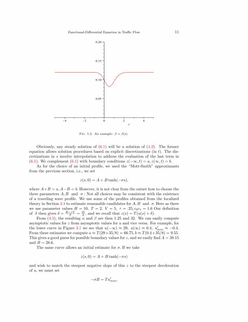
As for the choice of an initial profile, we used the “Mott-Smith” approximantsfrom the previous section, i.e., we set

z(s, 0) = A+B tanh(−σs),

where A+B = a,A−B = b. However, it is not clear from the outset how to choose thethree parameters A,B and σ : Not all choices may be consistent with the existenceof a traveling wave profile. We use some of the profiles obtained from the localizedtheory in Section 3.1 to estimate reasonable candidates for A,B and σ. Here as therewe use parameter values H = 10, T = 2, V = 5, τ = .25, c0c1 = 1.6 Our definitionof δ then gives δ = H−τV

T = 358 , and we recall that z(s) = T (u(s) + δ).

From (4.3), the resulting α and β are then 1.25 and 32. We can easily computeasymptotic values for z from asymptotic values for u and vice versa. For example, forthe lower curve in Figure 3.1 we see that u(−∞) ≈ 29, u(∞) ≈ 0.4, u′min ≈ −0.4.From these estimates we compute a ≈ T (29+35/8) = 66.75, b ≈ T (0.4+35/8) = 9.55.This gives a good guess for possible boundary values for z, and we easily find A = 38.15and B = 28.6.

The same curve allows an initial estimate for σ. If we take

z(s, 0) = A+B tanh(−σs)

and wish to match the steepest negative slope of this z to the steepest decelerationof u, we must set

−σB = Tu′min,


A 29.71 a 34.535B 4.825 b 24.885

u(−∞) 12.8925 u(∞) 8.067σ 0.0051 “time” step 0.04

Table 6.1Data for a “weak” jam

A 31.3055 a 44.2119B 12.9064 b 18.3991

u(−∞) 17.73095 u(∞) 4.82455σ 0.013061 “time” step 0.04

Table 6.2A stronger initial profile

or, for the data under consideration, σ = 0.02797. This same procedure can be appliedto all the possible triples (u(∞), u(−∞), u′min) arising from the theory in Section 3.1.Or, equivalently, one can compute localized traveling waves directly for the dependentvariable z(s); this is how the initial data in our first numerical experiment (the weakjam: see Table 6.1) were constructed.

We show the results of three different numerical experiments: “weak”, intermedi-ate and strong braking profiles. The relevant data are given in Tables 6.1 to 6.3. Inall runs we used α = 1.25, β = 32,∆t = 0.04,∆s = 8.5. The σ given in each table iscomputed as described above; if the limit state is stable, then the value of σ can bevaried without problems.

The braking wave corresponding to Table 6.1 is not depicted in Figure 3.1; it is a“weaker” wave in the sense that the speed difference is modest- the conversion givesu(−∞) ≈ 12.9, u(+∞) ≈ 8.07 (if we consider meters per second this translates intobraking modestly, from 46 to 29 km per hour).

The step size (8.5) seems large but works well because of the small slope in ourunits. We computed inside a domain (-15,000, + 2,000) in order to avoid boundaryerrors to invade (eventually, this is unavoidable, as our sought after waves are notconstant but only converge to constants for large |s| - in the simulations, one has touse a cutoff). The time step was 0.04. We used an adaptive upwind scheme withexcellent numerical stability. We are grateful for G. Russo for providing us with thescheme.

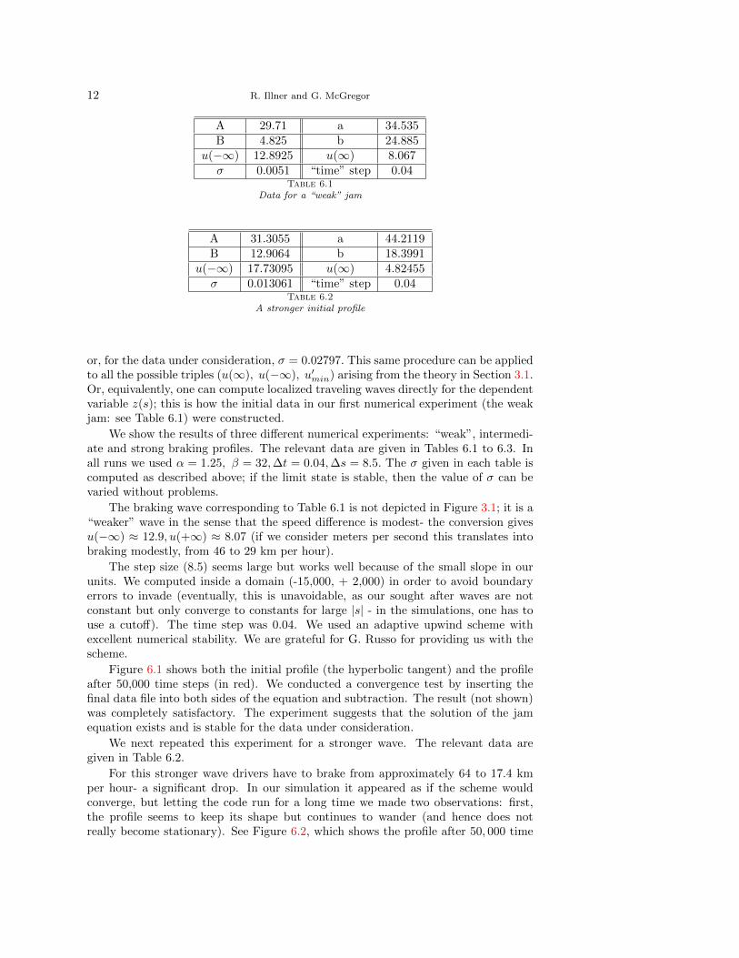
Figure 6.1 shows both the initial profile (the hyperbolic tangent) and the profileafter 50,000 time steps (in red). We conducted a convergence test by inserting thefinal data file into both sides of the equation and subtraction. The result (not shown)was completely satisfactory. The experiment suggests that the solution of the jamequation exists and is stable for the data under consideration.

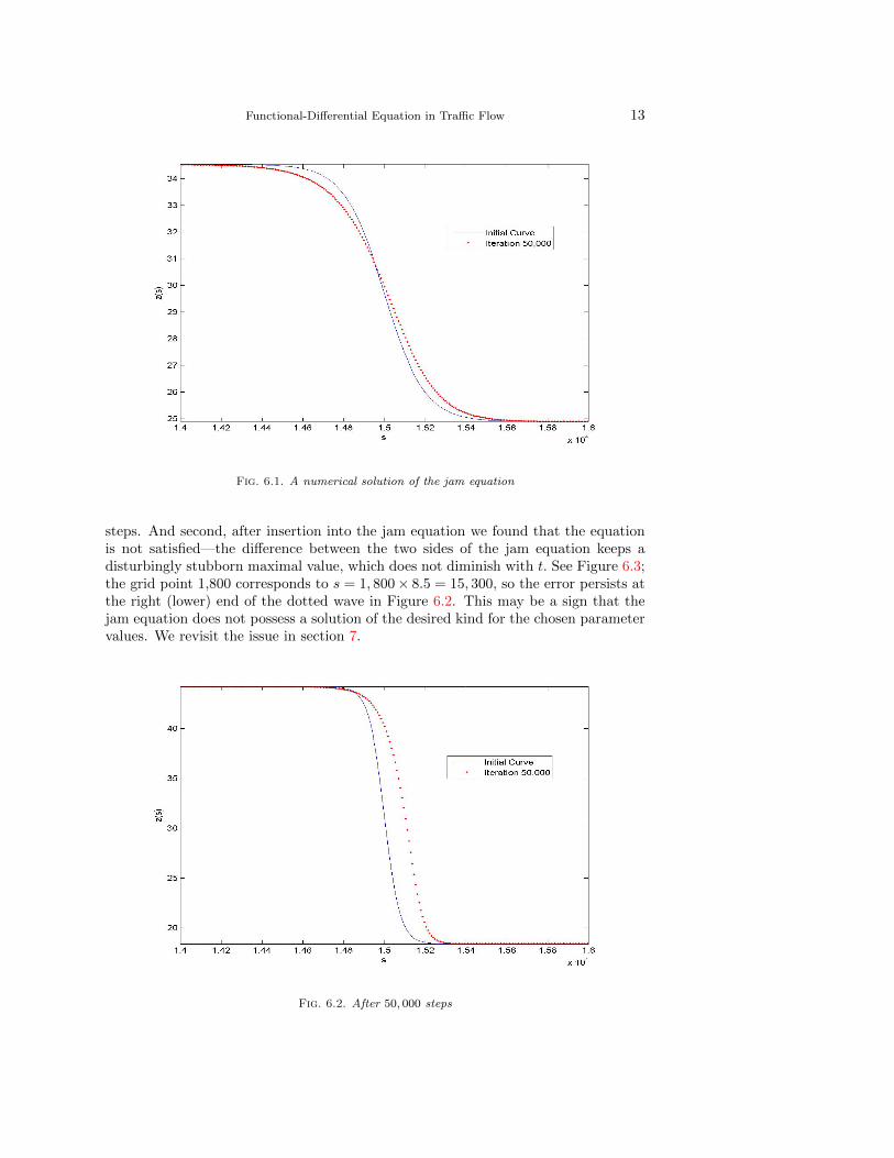
We next repeated this experiment for a stronger wave. The relevant data aregiven in Table 6.2.

For this stronger wave drivers have to brake from approximately 64 to 17.4 kmper hour- a significant drop. In our simulation it appeared as if the scheme wouldconverge, but letting the code run for a long time we made two observations: first,the profile seems to keep its shape but continues to wander (and hence does notreally become stationary). See Figure 6.2, which shows the profile after 50, 000 time


Fig. 6.1. A numerical solution of the jam equation

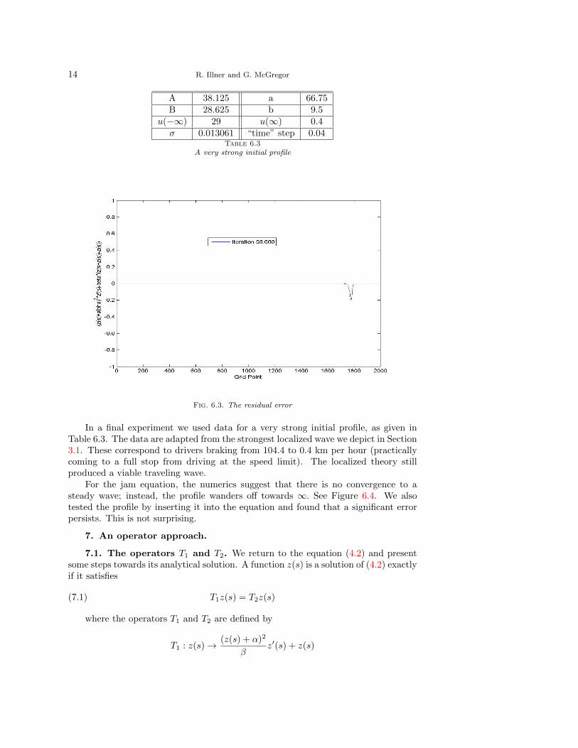
steps. And second, after insertion into the jam equation we found that the equationis not satisfied—the difference between the two sides of the jam equation keeps adisturbingly stubborn maximal value, which does not diminish with t. See Figure 6.3;the grid point 1,800 corresponds to s = 1, 800× 8.5 = 15, 300, so the error persists atthe right (lower) end of the dotted wave in Figure 6.2. This may be a sign that thejam equation does not possess a solution of the desired kind for the chosen parametervalues. We revisit the issue in section 7.

Fig. 6.2. After 50, 000 steps


A 38.125 a 66.75B 28.625 b 9.5

u(−∞) 29 u(∞) 0.4σ 0.013061 “time” step 0.04

Table 6.3A very strong initial profile

Fig. 6.3. The residual error

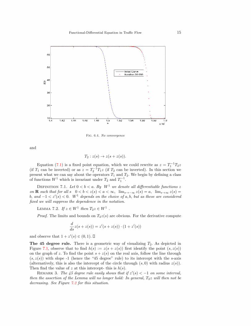
In a final experiment we used data for a very strong initial profile, as given inTable 6.3. The data are adapted from the strongest localized wave we depict in Section3.1. These correspond to drivers braking from 104.4 to 0.4 km per hour (practicallycoming to a full stop from driving at the speed limit). The localized theory stillproduced a viable traveling wave.

For the jam equation, the numerics suggest that there is no convergence to asteady wave; instead, the profile wanders off towards ∞. See Figure 6.4. We alsotested the profile by inserting it into the equation and found that a significant errorpersists. This is not surprising.

7. An operator approach.

7.1. The operators T1 and T2. We return to the equation (4.2) and presentsome steps towards its analytical solution. A function z(s) is a solution of (4.2) exactlyif it satisfies

T1z(s) = T2z(s)(7.1)

where the operators T1 and T2 are defined by

T1 : z(s)→ (z(s) + α)2

βz′(s) + z(s)


Fig. 6.4. No convergence

and

T2 : z(s)→ z(s+ z(s)).

Equation (7.1) is a fixed point equation, which we could rewrite as z = T−11 T2z(if T1 can be inverted) or as z = T−12 T1z (if T2 can be inverted). In this section wepresent what we can say about the operators T1 and T2. We begin by defining a classof functions W 1 which is invariant under T2 and T−11 .

Definition 7.1. Let 0 < b < a. By W 1 we denote all differentiable functions zon R such that for all s 0 < b < z(s) < a <∞, lims→−∞ z(s) = a, lims→∞ z(s) =b, and −1 < z′(s) < 0. W 1 depends on the choice of a, b, but as these are consideredfixed we will suppress the dependence in the notation.

Lemma 7.2. If z ∈W 1 then T2z ∈W 1 .

Proof. The limits and bounds on T2z(s) are obvious. For the derivative compute

d

dsz(s+ z(s)) = z′(s+ z(s)) · (1 + z′(s))

and observe that 1 + z′(s) ∈ (0, 1).

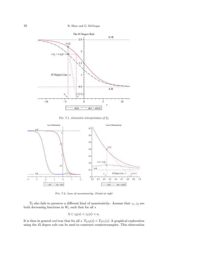
The 45 degree rule. There is a geometric way of visualizing T2. As depicted inFigure 7.1, observe that to find h(s) := z(s + z(s)) first identify the point (s, z(s))on the graph of z. To find the point s+ z(s) on the real axis, follow the line through(s, z(s)) with slope -1 (hence the “45 degree” rule) to its intercept with the s-axis(alternatively, this is also the intercept of the circle through (s, 0) with radius z(s)).Then find the value of z at this intercept- this is h(s).

Remark 3. The 45 degree rule easily shows that if z′(s) < −1 on some interval,then the assertion of the Lemma will no longer hold: In general, T2z will then not bedecreasing. See Figure 7.2 for this situation.


Fig. 7.1. Geometric interpretation of T2

Fig. 7.2. Loss of monotonicity. Detail at right

T2 also fails to preserve a different kind of monotonicity: Assume that z1, z2 areboth decreasing functions in W1 such that for all s

b < z2(s) < z1(s) < a.

It is then in general not true that for all s T2z2(s) < T2z1(s). A graphical explorationusing the 45 degree rule can be used to construct counterexamples. This observation


shows that it would be difficult to solve (4.2) using monotonicity methods.As T2 moves functions in W1 “to the left” and flattens them, T1 moves such

functions “down”. It is certainly plausible that T1 and T2 will have exactly the sameeffect on some functions (which, if true, would assert the existence of solutions to ourproblem).

While T1 moves z down it is not true that T1 maps W1 into itself. It is easy toconstruct examples of functions z in W1 for which, say, T1z violates the lower boundb. It turns out that a better way is to invert T1.

7.2. Inverting T1. The invertibility of T1 on the class W1 is given by the nexttheorem. Assume that h is continuous, strictly decreasing, and that h(−∞) = a >b = h(∞) > 0. We also recall that α and β are strictly positive constants.

Theorem 7.3. There is a unique function z = z(s) such that• (z + α)2z′ + βz = βh• z(−∞) = a, z(∞) = b• ∀s z′(s) < 0.

Observe that z = T−11 h.We remark that for the simpler linear case where z′+βz =βh a corresponding result holds, and it is easy to find an integral representation forz :

z(s) = β

∫ ∞0

e−βxh(s− x) dx.

The properties of z can be derived from this formula. The case at hand is moredifficult.

Proof. Uniqueness: from the equation it is clear that every solution with therequired properties will satisfy z > h (this follows from z = h − 1

β (z + α)2z′). Writethe equation as

d

ds

1

3(z(s) + α)3 = −β(z(s)− h(s)).

Integration gives

1

3

((b+ α)3 − (a+ α)3

)= −β

∫(z(s)− h(s)) ds.

The left-hand-side depends only on a and b. Therefore, if we had two solutions z1.z2,it would follow that

∫(z1(s)− z2(s)) ds = 0. By continuity there has to be a s0 where

z1(s0) = z2(s0), and this would imply z1 = z2 by the uniqueness theorem for ODEs.

Existence is a little less trivial, as we cannot start integration at ±∞. Instead,we use an approximation procedure. Choose a sequence (sn)n=1,2,... with sn → −∞,and consider for each n solutions zl, zh of the ODE with zl(sn) = h(sn), zh(sn) = a.These solutions are well defined everywhere, but we only consider them for s ≥ sn.For s < sn we set zh(s) ≡ a, zl(s) = h(s). This means that the approximants donot satisfy the equation for s ≤ sn. The functions zh and zl defined in this way arecontinuous and differentiable for s > sn, and they have the following properties.

a) for all s h(s) ≤ zl(s) ≤ zh(s) ≤ a, and for all s > sn h(s) < zl(s) < zh(s) < a.b) lims→∞ zh(s) = b = lims→∞ zl(s) = lims→∞ h(s). Similarly, all these limits

as s→ −∞ are a.


c) for s > sn z′l(s) < 0, z′h(s) < 0.

To prove these, note first that by uniqueness zh and zl cannot cross for s > sn.Further, zl cannot cross h, for if we had zl(t) = h(t) for some t > sn it would followfrom the equation that z′l(t) = 0 while h′(t) < 0, a contradiction. This shows a).Part c) is immediate from a) and from the equation. As for b), we only need to showthe first equality. Clearly, lims→∞ zh(s) exists. If this limit is, say, c > b, we integrateas before to find

1

3

(zh(s) + α)3 − (a+ α)3

)= −β

∫ s

sn

(zh(τ)− h(τ)) dτ

and observe that the integral will diverge as s→∞, a contradiction.To complete the proof we send n→∞, so sn → −∞. We obtain two sequences

of functions, znl (s) and znh (s), such that for s > sn

h(s) ≤ znl (s) < zn+1l (s) < zn+1

h (s) < znh (s) < a.

It follows that both sequences must converge uniformly to limits zl and zh, bothsolutions of the equation with the same boundary conditions. By uniqueness, itfollows that zl = zh. This completes the proof.

By the previous results the operator T2 maps W1 into itself, and T−11 is definedon W1. But it may well be that if h ∈ W1 then T−11 h /∈ W1 : the slope may becometoo steep. We next show that this will not happen if there are reasonable constraintson the parameters.

Lemma 7.4. Assume that β(a − b) ≤ (α + b)2. Then, if h ∈ W1 and z = T−11 hwe have z ∈W1.

Proof. All we have to do is to show that |z′(s)| ≤ 1. But from the equation for zwe have |z′|(z + α)2 = β|z − h| (observe that for all s we have z(s) > h(s).) Solvingfor |z′| we obtain

|z′| = β(z − h)

(z + α)2≤ β(a− b)

(b+ α)2≤ 1.

This result is straightforward and uses only the simplest estimates. Notice thatthe condition involves all four parameters. We can do better. Here is an alternativecondition, not involving the parameter a, giving the same result. We are grateful toour colleague Rod Edwards for showing us this condition.

Lemma 7.5. Suppose that β ≤ 2(b+ α). Then z ∈W1.

Proof. We will assume that z /∈W1 and show that then also h /∈W1. To this end,assume that there is a s1 such that z′(s1) < −1. From the differential equation it isclear that z′′ exists, and by differentiation we find

h′ = z′ +1

β[2(z′)2(z + α) + z′′(z + α)2].

We may further assume that s1 is the location where z′ assumes its minimum, andhence z′′(s1) = 0. Therefore


h′(s1) = z′(s1)

[1 +

2

βz′(s1)(z(s1) + α)

].

By using the assumption z′(s1) < −1 twice in the above identity we obtain theestimate

h′(s1) >2

β(z(s1) + α)− 1 >

2

β(b+ α)− 1 ≥ 0,

where the final estimate follows from the condition β ≤ 2(b + α). Hence h′(s1) > 0,contradicting h ∈W1.

Remark 4. It is instructive to test whether the parameter values used in thesimulations in Section 6 satisfy these conditions. A quick check shows that the datafrom Table 6.1 satisfy the conditions in both lemmas. The data from Table 6.2 violatesthe condition in Lemma 7.4 but satisifies the condition in Lemma 7.5, and the datafrom Table 6.3 violate both conditions.

If we assume that the parameter constraints from either lemma are satisfied, thenclearly T = T−11 T2 maps W1 into itself. Unfortunately, It does not seem to do socontractively, so we cannot use the Banach fixed point theorem to assert existenceof a fixed point. The Schauder fixed point theorem is also not directly applicable;the problem is that while W1 is a family of equicontinuous functions, it is not pre-compact because the domain is the whole real line, so the Arzela-Ascoli theorem isnot applicable in direct form. Regrettably, while we know that an iteratively definedsequence z0 := h ∈W1, zn+1 = Tzn will stay in W1, we cannot assert that there willbe a convergent subsequence. This difficulty is related to the translation invarianceof (4.2).

It is useful to visualize how the sequence {zn} could fail to converge: There couldbe a) progressive “flattening”, where the slopes of the zn would converge to zero oncompact subsets, and the zn themselves may (or may not) approach a constant in[b, a] on compact sets, while the boundary conditions are violated in the limit. Or,b) the wave could wander away to plus or minus infinity, leaving again a constantlimit a or b but violating one of the boundary conditions in the limit. One needsan additional compactness constraint to prevent this behaviour. A condition of thefollowing type suffices.

Assumption. Suppose that there is a nonempty subset W2 ⊂W1 with the followingtwo characteristics.

a) T : W2 →W2 (invariance under T )b) There are function hl, hu, both in W1, such that for all z ∈W2 and all s ∈ R

hl(s) ≤ z(s) ≤ hu(s).

The existence of such a W2 will certainly depend on the choice of parameters. Ifthere is such a set W2 then one can easily prove that W2 is compact with respect tothe topology of uniform convergence. Therefore, the Schauder fixed point theoremapplies on W2 to the operator T, and we have

Theorem 7.6. If a W2 with the properties a) and b) exists, then T has a fixedpoint in W2.


This result is not satisfactory, as we have no good criteria for the existence of sucha W2. Of course every fixed point itself is a possible element of such a set. Naturalcandidates for hl and hu are suitably scaled and shifted hyperbolic tangents (seeSection 5), i.e., hl(s) = A+B tanh(−σ1(s+s1)) and hu(s) = A+B tanh(−σ2(s−s1)),but it is not clear under which conditions the set {z ∈ W1;hl ≤ z ≤ hu} is invariantunder T2T

−11 . This is a challenge for the future; the numerical experiments from

Section 6 provide some guidance. For example, it seems reasonable to expect that aW2 as described will exists for the first example discussed there.

8. Concluding Remarks and an Applied Perspective. We have shown howthe “jam” equation (1.1) arises from a kinetic traffic model in a formal high-densitylimit (where traffic is locally synchronized) and via a travelling wave ansatz. Re-moving the non-locality via Taylor approximation provides easily solvable ordinarydifferential equations with convincing travelling wave profiles. Further, we investi-gated functional-differential equations similar to the jam equation from a geometricpoint of view, and we explored a hyperbolic-tangent approximation to the expectedwave profiles. Some numerical experiments were presented in Section 6. These experi-ments suggest that non-trivial solutions of (4.2) will exist for reasonable choices of thefour parameters (α, β, a, b) but not for all choices (for example, as seen in Figure 6.4,our numerical procedure may fail to converge and produce instead a profile wander-ing off to ∞. The functional-analytic discussion in Section 7 is consistent with theseobservations: we were able to identify non-trivial solutions of (4.2) as fixed points ofsuitable operators T1, T2 and managed to find function sets invariant under T−11 T2.This required constraints on the parameter set which are consistent with the resultsin Section 6. For the final Theorem we needed an additional invariance assumptionto overcome the lack of compactness in our function sets. It remains an interesting(and presumably hard) open problem to prove that this assumption really holds forsuitable parameters.

The applicability of our work is manifold: first, we obtained reasonable boundson the dimensions of possible wave speeds for traveling waves. Second, there is therelevance to identify accurate speed profiles in braking waves, which may prove usefulfor traffic guidance systems in congested domains (for example, optimal speed limitsto guarantee safety and maximize flux at the same time). Our models may also giveuseful information on boundary conditions (u(infty), u(∞)) for which traveling wavesexist.

A similar theory can be developed for acceleration waves. The localized versionof the corresponding “unjam” equation was already described in [14].

For practical purposes transition regimes between braking and acceleration willrequire additional modelling ingredients, because otherwise unrealistic behaviour mayresult. This is work in progress. For example, the model introduced in this paper cannaturally be coupled with the more common models where drivers are at liberty tobrake or accelerate according to a fundamental diagram.

9. Appendix. Here it is explained which parameter choices (α, a, b) will produceMott-Smith approximants for which β(−∞) = β(∞). Recall a = A + B, b = A − B.From the formula (5.2) for β(s) we have

β(−∞) = −σ(a+ α)2(1 + tanh(−σa))

tanh(−σa)


and

β(∞) = −σ(b+ α)2(1− tanh(−σb))tanh(−σb)

so both will be equal if (after multiplying both by σ)

(aσ + ασ)21− tanh (σa)

tanh (σa)= (bσ + ασ)2

1 + tanh (σb)

tanh (σb).(9.1)

So our question whether we can have a β(s) which approximates the same constant ass→ ±∞ will be answered in the affirmative if we find solutions of (9.1) in acceptableranges.

Proposition 9.1. Let σ > 0. Then (9.1) possesses solutions a > b > 0 if α > 0is sufficiently small (relative to σ).

Proof. First note that σ scales all the variables (α, a, b) in (9.1). We can thereforejust set σ = 1. Then (9.1) simplifies to

(a+ α)21− tanh a

tanh a= (b+ α)2

1 + tanh b

tanh b.(9.2)

For α = 0 the right-hand side is b2(1 + tanh b)/ tanh b, and by L’Hopital’s rulelimb→0 b

2(1 + tanh b)/ tanh b = 0. Therefore, for all ε > 0 there is an α(ε) such thatfor all α < α(ε)

infb>0

(α+ b)2(1 + tanh b)/ tanh b ≤ ε,

although

limb→0

(α+ b)2(1 + tanh b)/ tanh b =∞.

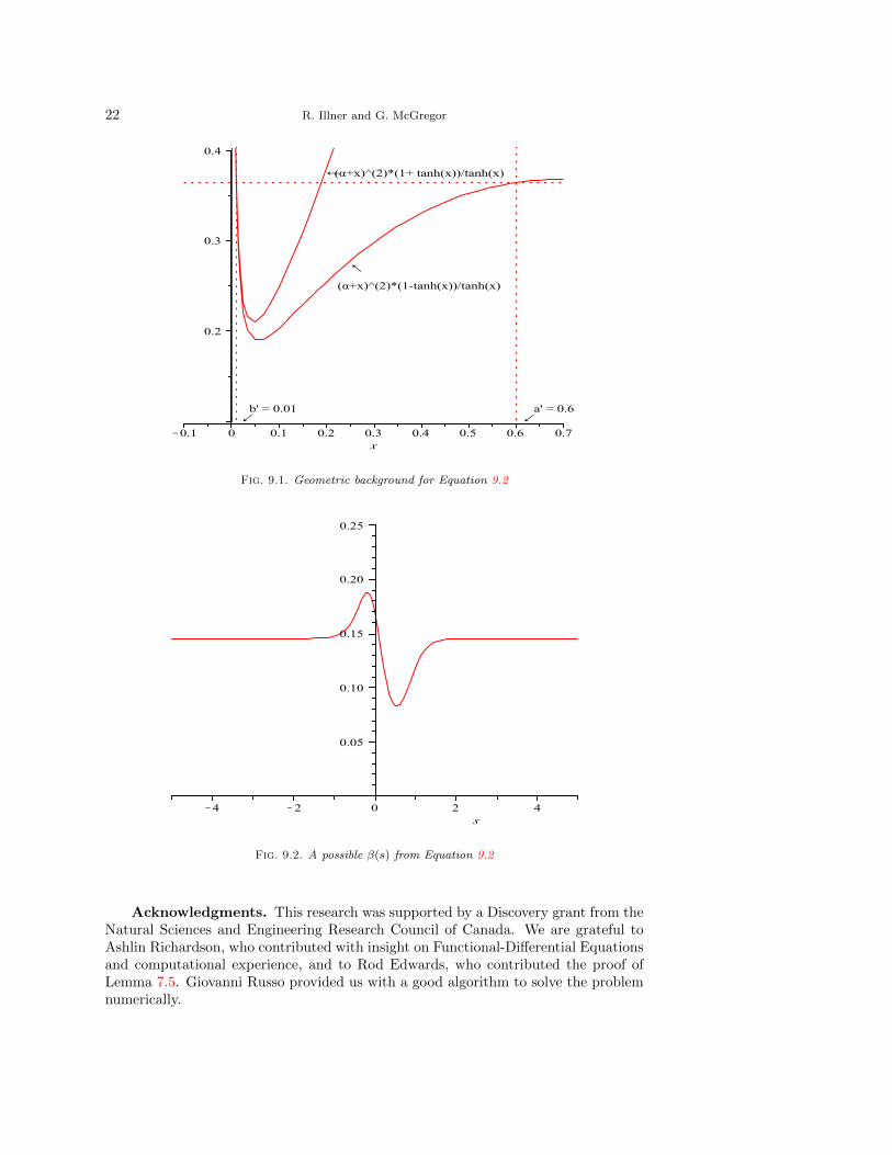
The two sides of equation (9.2) are depicted in Figure 9.1, where x is written for a andb respectively. For small enough α there is an interval (dependent on α) I := [a1, a2]such that the left-hand side of (9.2) is increasing as a function of a on I, and

mina∈I

(a+ α)2(1− tanh a)/ tanh a ≥ minb>0

(b+ α)2(1 + tanh b)/ tanh b.

For each a ∈ I there are then 2 values for b (one for a = a1) such that (9.2) holds.See Figure 9.1.

The corresponding β(s) for a = 0.6, b = 0.01, σ = 1 and α = 0.05 is plotted inFigure 9.2


Fig. 9.1. Geometric background for Equation 9.2

Fig. 9.2. A possible β(s) from Equation 9.2

Acknowledgments. This research was supported by a Discovery grant from theNatural Sciences and Engineering Research Council of Canada. We are grateful toAshlin Richardson, who contributed with insight on Functional-Differential Equationsand computational experience, and to Rod Edwards, who contributed the proof ofLemma 7.5. Giovanni Russo provided us with a good algorithm to solve the problemnumerically.


REFERENCES

[1] A. Aw and M. Rascle, Resurrection of “second order” models of traffic flow., SIAM J. Appl.Math., 60 (2000), pp. 916–938.

[2] E. Ben-Naim, P. L. Krapinsky, S. Redner, Kinetics of clustering in traffic flows, PhysicalRev. E 50(2), (1994) pp. 822–829.

[3] S. S. Cheng, W. Li, Analytic Solutions of Functional Equations, World Scientific (2008)[4] C. Cercignani, A. Frezzotti, P. Grosfils, The structure of an infinitely strong shock wave,

Phys. Fluids 11, (1999), 2757–2765.[5] J. Dolbeault and R. Illner, Entropy methods for kinetic models of traffic flow, Commun.

Math. Sci, 1 (2003), pp. 401–423.[6] I. Gasser, T. Seidel, G. Sirito, and B. Werner, Bifurcation Analysis of a Class of Car

Following Traffic Models II: Variable Reaction Times and Agressive Drivers, Bulletin ofthe Institute of Mathematics, Academica Sinica (New Series), 2 (2007), pp. 587–607.

[7] I. Gasser, G. Sirito, and B. Werner, Bifurcation analysis of a class of ‘car following’ trafficmodels., Physica D, 197 (2004), pp. 222–241.

[8] J. Greenberg, Extensions and amplifications of a traffic model of Aw and Rascle., SIAM J.Appl. Math., 62 (2001), pp. 729–745.

[9] , Congestion redux., SIAM J. Appl. Math., 64 (2004), pp. 1175–1185.[10] , Traffic congestion – an instability in a hyperbolic system, Bulletin of the Institute of

Mathematics, Academica Sinica (New Series), 2 (2007), pp. 123–138.[11] J. Greenberg, A. Klar, and M. Rascle, Congestion on multilane highways., SIAM J. Appl.

Math., 63 (2003), pp. 818–833.[12] D. Helbing, Traffic dynamics. New physical concepts of modelling. (Verkehrsdynamik. Neue

physikalische Modellierungskonzepte.), Berlin: Springer. xii, 308 p. DM 128.00; oS 934.40;sFr 113.00 , 1997.

[13] D. Helbing, A. Hennecke, V. Shvetsov, and M. Treiber, Micro- and macro-simulation offreeway traffic., Math. Comput. Modelling, 35 (2002), pp. 517–547.

[14] M. Herty, R. Illner,On stop-and-go waves in dense traffic., Kinetic and Related Models1(3)(2008), pp. 437-452.

[15] M. Herty, R. Illner, Analytical and numerical investigations of refined macroscopic traffic flowmodels, Kinetic and Related Models 2(3) (2010), pp. 311-334.

[16] M. Herty, R. Illner, A. Klar, and V. Panferov, Qualitative properties of solutions tosystems of Fokker-Planck equations for multilane traffic flow., Transp. Theory Stat. Phys.,35 (2006), pp. 31–54.

[17] M. Herty and A. Klar, Modelling, simulation and optimization of traffic flow networks,SIAM J. Sci. Comp., 25 (2003), pp. 1066-1087.

[18] M. Herty and M. Rascle, Coupling conditions for a class of second-order models for trafficflow. , SIAM J. Math. Anal., 38 (2006), pp. 595-616.

[19] R. Illner, C. Kirchner, and R. Pinnau, A derivation of the Aw–Rascle traffic models fromfokker-planck type kinetic models, Quarterly Appl. Math., 67(1) (2009), pp. 39–45

[20] R. Illner, A. Klar, and T. Materne, Vlasov-Fokker-Planck models for multilane trafficflow., Commun. Math. Sci., 1 (2003), pp. 1–12.

[21] A. Klar, R .Wegener, A hierarchy of models for multilane vehicular traffic. I. Modeling.,SIAM J. Appl. Math., Vol. 3 (1999), pp. 983–1001

[22] B. Kerner, The Physics of traffic, Springer, Berlin, 2004.[23] J. P. Lebacque, Les modeles macroscopiques de trafic, Annales des Ponts 67, 3rd trim, (1993),

pp 28-45.[24] P. I. Richards, Shock waves on the highway, Oper. Res., 4 (1956), pp. 42–51.[25] A. Richardson, M.Sc. Thesis, University of Victoria (2011), in preparation.[26] L. Santen, A. Schadschneider, M. Schreckenberg, Towards a realistic microscopic de-

scription of highway traffic, J. Phys A, Vol. 33, (2000), pp. 477–485[27] S. Marinosson, R. Chrobok, A. Pottmeier, J. Wahle, M. Schreckenberg, Simulation

framework for the autobahn traffic in North Rhine-Westphalia, Cellular automata 315–324, Lecture Notes in Comput. Sci., 2493, Springer, Berlin (2002)

[28] T. Alperovich, A. Sopasakis, Stochastic description of traffic flow, J. Stat. Phys., Vol. 133(2008), pp. 1083-1105

[29] A. Sopasakis, M.A. Katsoulakis, Stochastic modeling and simulation of traffic flow: asym-metric single exclusion process with Arrhenius look-ahead dynamics, SIAM J. Appl. Math.,Vol. 66 (2006), pp. 921-944.

[30] M. Treiber and D. Helbing, Macroscopic simulation of widely scattered synchronized trafficstates., J. Phys. A, Math. Gen., (1999).


[31] H. M. Zhang, A non–equilibrium traffic model devoid of gas–like behavior, Tans. Res. B, Vol.36 (2002), pp. 275–290

Received xxxx 20xx; revised xxxx 20xx.

Documents

ON A FUNCTIONAL-DIFFERENTIAL EQUATION ARISING FROM … · ON A FUNCTIONAL-DIFFERENTIAL EQUATION ARISING FROM ... The model is related to the macroscopic tra c model rst suggested