on a circle with point singularities - arXiv · on a circle with point singularities ... [email protected] ... the upper ﬁgures mean the geometrical meaning of Pk,Rk

arX

iv:h

ep-t

h/05

0513

2v3

3 A

ug 2

005

KOBE-TH-05-03OU-HET-530

Extended supersymmetry and its reductionon a circle with point singularities

Tomoaki Nagasawa1, Makoto Sakamoto2, Kazunori Takenaga3

1Graduate School of Science and Technology, Kobe University, Rokkodai, Nada,

Kobe 657-8501, Japan2Department of Physics, Kobe University, Rokkodai, Nada, Kobe 657-8501, Japan

3Department of Physics, Osaka University, Toyonaka 560-0043, Japan

Abstract

We investigate N -extended supersymmetry in one-dimensional quan-

tum mechanics on a circle with point singularities. For any integer n,

N = 2n + 1 supercharges are explicitly constructed in terms of discrete

transformations, and a class of singularities compatible with supersym-

metry is clarified. In our formulation, the supersymmetry can be reduced

to M-extended supersymmetry for any integer M < N . The degener-

acy of the spectrum and spontaneous supersymmetry breaking are also

studied.

1 Introduction

A point singularity in one dimensional quantum mechanics may be considered, in general,

as a localized limit of a finite range potential and is parametrized by the group U(2)[1, 2, 3],

and the parameters characterize connection conditions between a wavefunction and its

derivative at the singularity. The varieties of the connection conditions lead to various

interesting phenomena, such as duality[4, 5], the Berry phase[6, 7], scale anomaly[8] and

supersymmetry[9, 10, 11, 12].

N = 1 or N = 2 supersymmetry in the model of a free particle on a line R or an1e-mail: [email protected] (T. Nagasawa)2e-mail: [email protected] (M. Sakamoto)3e-mail: [email protected] (K. Takenaga)

1

http://arxiv.org/abs/hep-th/0505132v3

interval [−l, l] with a point singularity was discussed in Ref. [9]. In Ref. [11], this work was

extended to N = 4 supersymmetry in the model on a pair of lines or intervals each having

a point singularity. In Ref. [10], N = 2 supersymmetric model with a superpotential was

constructed on a circle with two point singularities. The supercharges are represented in

terms of a set of discrete transformation {P1,Q1,R1}, which forms an su(2) algebra of

spin 1/2. In Ref. [12], this work was extended to N = 2n supersymmetry by putting

2n number of point singularities on a circle, and N = 2n supercharges are explicitly

constructed in terms of n sets of discrete transformations {P1,Q1,R1}, · · · , {Pn,Qn,Rn}on the circle.

We would like to emphasize that the study on the supersymmetry in one dimensional

quantum mechanics with point singularities has a physical application to higher dimen-

sional gauge theories. It has been shown that a quantum-mechanical supersymmetry is

hidden in any gauge invariant theories with extra dimensions[13, 14, 15]. In Ref. [14],

the hierarchy problem at tree level has been solved in a scenario of gauge theories with

compact extra dimensions with boundaries[16]. Then, the hidden quantum-mechanical

supersymmetric structure as well as the choice of boundary conditions have been found

to be crucial, and the analyses in Ref. [10, 12] have turned out to give a powerful tool to

derive all possible sets of boundary conditions.

In this paper, we study N = 2n + 1 supersymmetry on a circle with 2n point singu-

larities, and give a full detail of the analysis. The N = 2n+ 1 supercharges are explicitly

constructed in terms of n + 1 sets of discrete transformations

{P1,Q1,R1}, · · · , {Pn,Qn,Rn}, {Pn+1,Qn+1,Rn+1}.

Since the model contains point singularities, we need to impose appropriate connection

conditions there. We succeed to clarify a possible set of connection conditions compatible

with the N = 2n+1 supercharges. Thus, the N = 2n+1 supersymmetry can be realized

under the connection conditions. In our formulation, we can remove some of the N = 2n+

1 supercharges from a class of physical observables by relaxing the connection conditions,

so that the N = 2n + 1 supersymmetry can be reduced to M-extended supersymmetry

for any integer M < N . This implies that for any fixed M we have a wide variety of

M-extended supersymmetric models. We provide a general discussion about reduction

of the supersymmetry and construct N = 2n supersymmetric models as a result of the

reduction of the original N = 2n+ 1 supersymmetry. We also investigate the degeneracy

of the spectrum, in particular, vacuum states with vanishing energy.

The plan of this paper is as follows. In Section 2, we introduce n + 1 sets of discrete

transformations on a circle. In Section 3, we construct N = 2n+1 supercharges in terms

of these discrete transformations and examine connection conditions compatible with all

the 2n+ 1 supercharges. We also investigate the degeneracy of the spectrum. In Section

4, we discuss reduction of the supersymmetry and study some N = 2n supersymmetric

models as examples. Section 5 is devoted to summary.

2

x l0= l=

1x l= l= ( )1– 1

2n 1–—

3x l= l= ( )1–3

2 n 1–—

2x l= l= ( )1–

2

2n 1–—

x l2= n =–22

l—

x l2= n 1– =0

x l2

= n=–1 2

l—–32–

.

2x l= –1n = l( )–1 + 1

2n 1–—

2x l= –2n l= ( )–1 + 2

2n 1–—

2x l= –3n l= ( )–1 +

3

2n 1–—

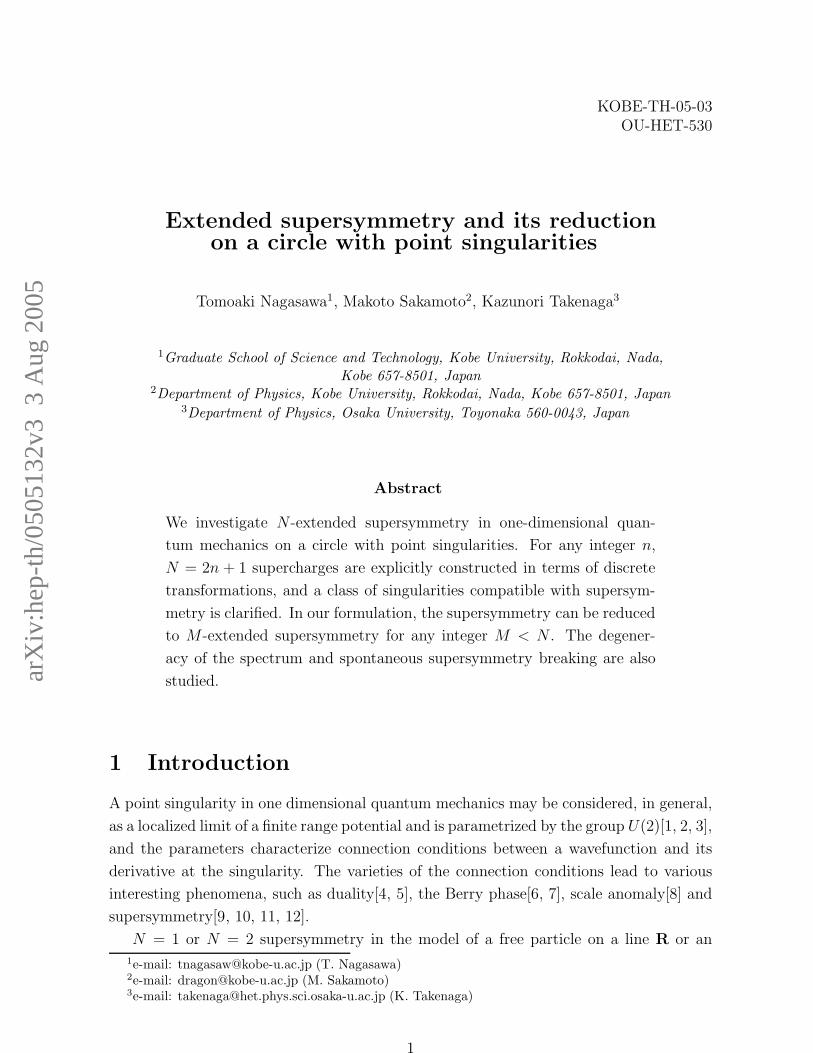
Figure 1: The positions of the singularities on a circle S1(−l < x ≤ l)

2 Discrete transformations

We consider the model which is one-dimensional quantum mechanics on a circle S1 (−l <x ≤ l) with 2n point singularities placed at

x = ls ≡(

1− s

2n−1

)

l for s = 0, 1, · · · , 2n − 1. (2.1)

This paper deals with the model in which the wavefunction and its derivative are contin-

uous everywhere except for the point singularities. These point singularities are placed at

regular intervals on the circle (Fig. 1). We define discrete transformations on the circle

as

(Pkϕ)(x) =2k−1∑

s=1

Θ(

x−(

1− s

2k−2

)

l)

Θ((

1− s− 1

2k−2

)

l − x)

×ϕ(

−x+(

2− 2s− 1

2k−1

)

l)

, (2.2)

3

(Rkϕ)(x) =2k−1∑

s=1

(−1)s[

−Θ

(

x−(

1− s− 1/2

2k−2

)

l

)

Θ((

1− s− 1

2k−2

)

l − x)

+ Θ(

x−(

1− s

2k−2

)

l)

Θ

((

1− s− 1/2

2k−2

)

l − x

)]

ϕ(x),

(2.3)

(Qkϕ)(x) ≡ −i (RkPkϕ) (x) (2.4)

for k = 1, 2, · · · , n+ 1. Here Θ(x) is the Heaviside step function defined by

Θ(x) =

{

1 for 0 < x < l,0 for −l < x < 0.

(2.5)

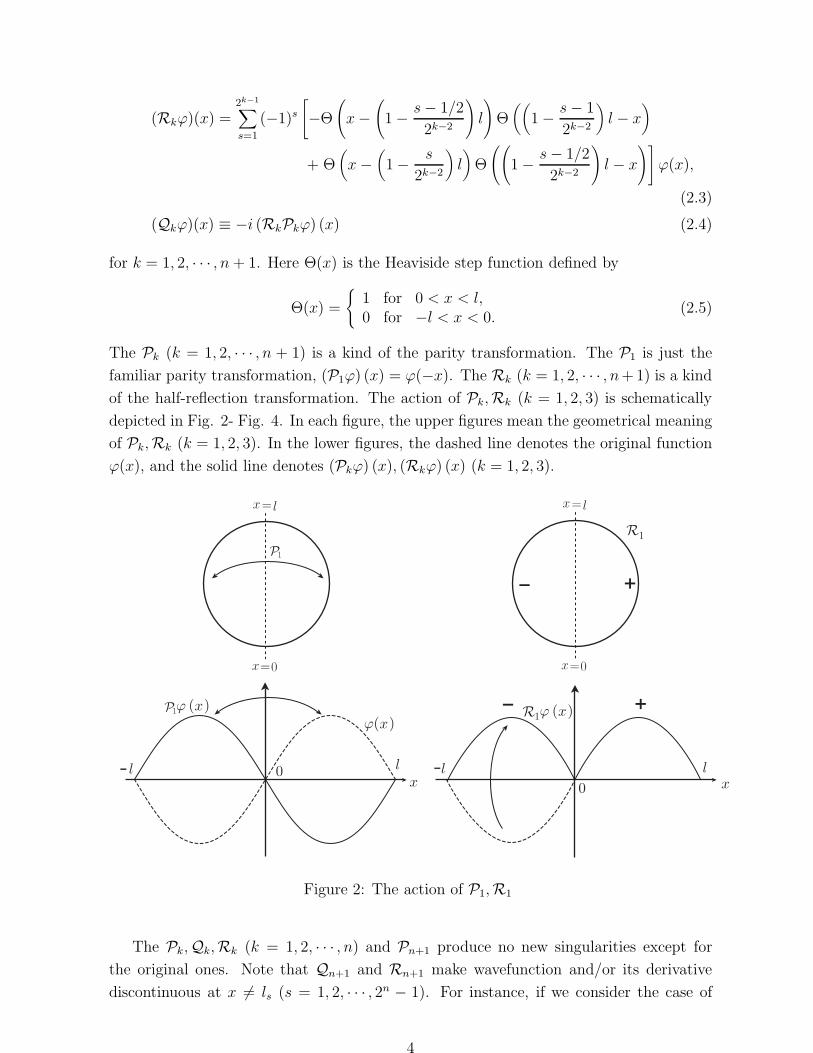
The Pk (k = 1, 2, · · · , n + 1) is a kind of the parity transformation. The P1 is just the

familiar parity transformation, (P1ϕ) (x) = ϕ(−x). The Rk (k = 1, 2, · · · , n+1) is a kind

of the half-reflection transformation. The action of Pk,Rk (k = 1, 2, 3) is schematically

depicted in Fig. 2- Fig. 4. In each figure, the upper figures mean the geometrical meaning

of Pk,Rk (k = 1, 2, 3). In the lower figures, the dashed line denotes the original function

ϕ(x), and the solid line denotes (Pkϕ) (x), (Rkϕ) (x) (k = 1, 2, 3).

1R

llxx

ll -- 00

ϕ( )x

ϕ ( )x ϕ ( )x1R

Figure 2: The action of P1,R1

The Pk,Qk,Rk (k = 1, 2, · · · , n) and Pn+1 produce no new singularities except for

the original ones. Note that Qn+1 and Rn+1 make wavefunction and/or its derivative

discontinuous at x 6= ls (s = 1, 2, · · · , 2n − 1). For instance, if we consider the case of

4

ll

l

lxx -

-

R2

00

ϕ ( )xR2

ϕ ( )x2

ϕ( )x


R3

3

ϕ ( )xR3

0 l xl

l l--x

0

ϕ( )x

ϕ ( )x ϕ( )x


5

n = 1, there are two singularities located at x = 0, l. As seen in fig. 2, a set of discrete

transformation {P1,Q1,R1} does not make wavefunction and its derivative discontinuous

at x 6= 0, l. We introduce a new set of discrete transformation {P2,Q2,R2}. Although

the P2 produces no new discontinuity for wavefunction and its derivative at x 6= 0, l, the

Q2 and R2, however, produce discontinuity for wavefunction and/or its derivative at the

different points of the original singularities, x = ± l2(see fig. 3).

A crucial observation is that each set {Pk,Qk,Rk} (k = 1, 2, · · · , n+1) forms an su(2)

algebra of spin 1/2,

PkQk = −QkPk = iRk, QkRk = −RkQk = iPk, RkPk = −PkRk = iQk,

(Pk)2 = (Qk)2 = (Rk)

2 = 1 (2.6)

and that Ok = {Pk,Qk,Rk} and Ok′ = {Pk′,Qk′,Rk′} commute with each other if k 6= k′,

[Ok,Ok′ ] = 0 for k 6= k′. (2.7)

For later use, let us introduce new sets of su(2) generators {GPk,GQk

,GRk} (k =

1, 2, · · · , n) as

GPk= V†PkV, GQk

= V†QkV, GRk= V†RkV, k = 1, 2, · · · , n, (2.8)

where

V ≡ V1V2 · · · Vn, Vk = ei~vk ·~Pk ∈ SU(2). (2.9)

Here, ~Pk (~vk) is an abbreviation of ~Pk = (Pk,Qk,Rk) (~vk = (vPk, vQk

, vRk)), and (vPk

, vQk, vRk

)

are real parameters. The new su(2) generators {GPk,GQk

,GRk} have to be linearly related

to ~Pk as

GPk= ~ePk

· ~Pk, GQk= ~eQk

· ~Pk, GRk= ~eRk

· ~Pk, k = 1, 2, · · · , n, (2.10)

where {~ePk, ~eQk

, ~eRk} are three-dimensional orthogonal unit vectors.

3 N = 2n+ 1 supersymmetry

3.1 N = 2n + 1 supercharges

Equipped with the discrete transformations given in the previous section, we construct

N = 2n+1 supercharges in terms of the n+1 sets of the discrete transformations. There

are two types of N = 2n+ 1 supercharges (type A and type B),

• Type A

QAa =

i

2ΓaDA =

i

2DAΓa, a = 1, 2, · · · , 2n+ 1, (3.1)

6

• Type B

QBa =

i

2ΓaDB =

i

2DBΓa, a = 1, 2, · · · , 2n+ 1, (3.2)

where

DA =

(

R1 · · ·Rn+1d

dx

)

+ GR1 · · · GRn(R1 · · ·Rn+1W

′(x)) , (3.3)

DA =

(

R1 · · ·Rn+1d

dx

)

− GR1 · · · GRn(R1 · · ·Rn+1W

′(x)) , (3.4)

DB =

(

R1 · · ·Rn+1d

dx

)

− Pn+1 (R1 · · ·Rn+1V′(x)) , (3.5)

DB =

(

R1 · · ·Rn+1d

dx

)

+ Pn+1 (R1 · · ·Rn+1V′(x)) (3.6)

and

Γ2k−1 = GR1GR2 · · · GRk−1GPk

Rn+1,Γ2k = GR1GR2 · · · GRk−1

GQkRn+1, k = 1, 2, · · · , n,

Γ2n+1 = Qn+1.(3.7)

Here, W ′(x) = ddxW (x), V ′(x) = d

dxV (x), and W (x), V (x) are called superpotentials. We

note that Γa,DA(B), DA(B) in the supercharges contain Rn+1,Qn+1 which produce new

singularities except for the original singular point x = ls(s = 1, 2, · · · , 2n − 1). The

combinations of these operators in the supercharges, however, make the Qn+1 and Rn+1

vanished due to the su(2) algebra.

The functions W ′(x), V ′(x) are continuous and finite valued functions at intervals

between singularities and are allowed to have discontinuities at x = ls (s = 0, 1, · · · , 2n−1).

In order to construct the N = 2n+ 1 superalgebra, the functions turn out to be required

to

PkW ′(x) = −W ′(x)Pk, k = 1, 2, · · · , n, (3.8)

Pn+1W′(x) = W ′(x)Pn+1 (3.9)

and

PiV ′(x) = −V ′(x)Pi, i = 1, 2, · · · , n+ 1. (3.10)

Noting thatR1 · · ·Rn+1ddx,R1 · · ·Rn+1W

′(x) andR1 · · ·Rn+1V′(x) commute with {Pk,Qk,Rk}

(k = 1, 2, · · · , n+ 1), we have the relations

{Γa,Γb} = 2δab, (3.11)

ΓaDA(B) = DA(B)Γa, a, b = 1, 2, · · · , 2n+ 1. (3.12)

It follows that the supercharges form the N = 2n+ 1 superalgebra;

7

• Type A

{QAa , Q

Ab } = HAδab, a, b = 1, 2, · · ·2n+ 1, (3.13)

HA = −1

2DADA =

1

2

[

− d2

dx2− GR1 · · · GRn

W ′′(x) + (W ′(x))2

]

, (3.14)

• Type B

{QBa , Q

Bb } = HBδab, a, b = 1, 2, · · ·2n+ 1, (3.15)

HB = −1

2DBDB =

1

2

[

− d2

dx2+ Pn+1V

′′(x) + (V ′(x))2

]

, (3.16)

where HA and HB are the Hamiltonian in each model.

3.2 Connection conditions compatible with supersymmetry

In this section, we clarify the connection conditions compatible with the N = 2n + 1

supersymmetry. Since the model contains the point singularities, we need to impose

appropriate connection conditions there, namely, our model is specified not only by the

Hamiltonian but also by the connection conditions. The functional space in our model is

required to be squared integrable and to be spanned by eigenfunctions of the Hamiltonian

with connection conditions that make the Hamiltonian hermitian.

In order to obtain the appropriate connection conditions, let us introduce a 2n+1 -

dimensional boundary vector Φϕ that consists of boundary values of a wavefunction ϕ(x)

in the vicinity of the singularities, ϕ(ls ± ǫ) for s = 0, 1, · · · , 2n − 1 with an infinitesimal

positive constant ǫ. For later convenience, we arrange ϕ(ls ± ǫ) in such a way that Φϕ

satisfies the relations

ΦPkϕ = (

k︷︸︸︷

I2 ⊗ · · · ⊗ I2 ⊗ σ1 ⊗I2 ⊗ · · · ⊗ I2)Φϕ, (3.17)

ΦQkϕ = (I2 ⊗ · · · ⊗ I2 ⊗ σ2 ⊗ I2 ⊗ · · · ⊗ I2)Φϕ, (3.18)

ΦRkϕ = (I2 ⊗ · · · ⊗ I2 ⊗ σ3 ⊗ I2 ⊗ · · · ⊗ I2︸︷︷︸

n+1

)Φϕ, (3.19)

where IM denotes anM×M unit matrix, and σi(i = 1, 2, 3) stands for the Pauli matrices.

8

The boundary vector can be arranged as

Φϕ =

ϕ(l0 − ǫ)ϕ(l1 + ǫ)

(Pnϕ)(l0 − ǫ)(Pnϕ)(l1 + ǫ)(Pn−1ϕ)(l0 − ǫ)(Pn−1ϕ)(l1 + ǫ)

(Pn−1Pnϕ)(l0 − ǫ)(Pn−1Pnϕ)(l1 + ǫ)(Pn−2ϕ)(l0 − ǫ)(Pn−2ϕ)(l1 + ǫ)

(Pn−2Pnϕ)(l0 − ǫ)(Pn−2Pnϕ)(l1 + ǫ)(Pn−2Pn−1ϕ)(l0 − ǫ)(Pn−2Pn−1ϕ)(l1 + ǫ)

(Pn−2Pn−1Pnϕ)(l0 − ǫ)(Pn−2Pn−1ϕ)(l1 + ǫ)

...(P2P3 · · · Pnϕ)(l0 − ǫ)(P2P3 · · · Pnϕ)(l1 + ǫ)

· · · · · · · · · · · · · · ·P1

[

upper halfcomponents

]

. (3.20)

For instance, Φϕ for the case of n = 1 (two singular points are placed at x = 0, l) is

arranged as

Φϕ =

ϕ(l − ǫ)ϕ(0 + ǫ)ϕ(−l + ǫ)ϕ(0− ǫ)

=

ϕ(l − ǫ)ϕ(0 + ǫ)

(P1ϕ)(l − ǫ)(P1ϕ)(0 + ǫ)

, (3.21)

which obeys the relations (3.17)-(3.19) with n = 1,

ΦP1ϕ =

(P1ϕ) (l − ǫ)(P1ϕ) (0 + ǫ)(P1ϕ) (−l + ǫ)(P1ϕ) (0− ǫ)

=

ϕ(−l + ǫ)ϕ(0− ǫ)ϕ(l − ǫ)ϕ(0 + ǫ)

=

(

0 I2I2 0

)

Φϕ = (σ1 ⊗ I2)Φϕ,

(3.22)

ΦR1ϕ =

(R1ϕ) (l − ǫ)(R1ϕ) (0 + ǫ)(R1ϕ) (−l + ǫ)(R1ϕ) (0− ǫ)

=

ϕ(l − ǫ)ϕ(0 + ǫ)

−ϕ(−l + ǫ)−ϕ(0− ǫ)

=

(

I2 00 −I2

)

Φϕ = (σ3 ⊗ I2)Φϕ,

(3.23)

9

ΦQ1ϕ =

(Q1ϕ) (l − ǫ)(Q1ϕ) (0 + ǫ)(Q1ϕ) (−l + ǫ)(Q1ϕ) (0− ǫ)

=

−iϕ(−l + ǫ)−iϕ(0− ǫ)iϕ(l − ǫ)iϕ(0 + ǫ)

=

(

0 −iI2iI2 0

)

Φϕ = (σ2 ⊗ I2)Φϕ.

(3.24)

Since our model has the singular points, wavefunction will, in general, be discontinuous

there, but the discontinuity has to be controlled by the connection conditions that make

the Hamiltonian hermitian. The hermiticity condition is

∫ l

−ldxψ∗(x)

(

HA(B)ϕ)

(x) =∫ l

−ldx(

HA(B)ψ)∗

(x)ϕ(x) (3.25)

for any wavefunctions ψ(x), ϕ(x), where the integral∫ l−l dx is defined by

∫ l

−ldx ≡

2n∑

s=1

∫ ls−1−ǫ

ls+ǫdx with l2n ≡ l0. (3.26)

In terms of the boundary vector, the requirement (3.25) can simply be rewritten as the

constraints on the boundary vector

Φ†ψΦDA(B)ϕ = Φ†

DA(B)ψΦϕ. (3.27)

In order to derive it, we have used the relation (3.19) and the formula of integration by

parts

∫ l

−ldxξ∗(x)

(

d

dxη(x)

)

= −∫ l

−ldx

(

d

dxξ(x)

)∗

η(x) + Φ†ξ(σ3 ⊗ · · · ⊗ σ3)Φη, (3.28)

where the functions ξ(x) and η(x) are assumed to be continuous everywhere except for

the singular points. It is easy to show that eq. (3.27) is equivalent to

|Φϕ − iL0ΦDA(B)ϕ| = |Φϕ + iL0ΦDA(B)ϕ|, (3.29)

where L0 is an arbitrary nonzero constant with the dimension of length. Then, the

condition (3.29) can be written as

(I2n+1 − U) Φϕ + iL0 (I2n+1 + U) ΦDA(B)ϕ = 0, (3.30)

where U is a 2n+1×2n+1 unitary matrix. Thus, we have found that the connection condi-

tions which make the Hamiltonian hermitian are given by eq. (3.30). The 2n singularities

in our model are characterized by a 2n+1 × 2n+1 unitary matrix, U .

It is important to notice that the above connection condition does not necessarily

guarantee the N = 2n + 1 supersymmetry, because the hermiticity of the Hamiltonian

does not, in general, ensure that of the supercharges. Moreover, the state, (Qaϕ) (x)

does not necessarily belong to the same functional space as ϕ(x). This also means that

10

(Qaϕ) (x) does not obey the same connection conditions as ϕ(x). In order for any operator

O to be physical, the state (Oϕ) (x) for any state ϕ(x) has to obey the same connection

conditions as ϕ(x). In the following, we call O a physical operator if O is hermitian and

(Oϕ) (x) satisfies the same connection conditions as ϕ(x).

In the standard argument of supersymmetry, for any energy eigenfunction ϕ with an

energy E, Qaϕ is also an energy eigenfunction with the same energy E(> 0) and then Qaϕ

is called a supersymmetric partner of ϕ. In our model, this is true if and only if Qa is a

physical operator, otherwise the state Qaϕ should be removed from the functional space,

in which any state satisfies the connection conditions (3.30) with a characteristic matrix

U . Therefore the N = 2n + 1 supersymmetry can be realized in our model, only when

all the N = 2n + 1 supercharges are physical. We will see below that this requirement

severely restricts a class of the connection conditions.

Let ϕ(x) be any wavefunction obeying the connection conditions (3.30), and satisfying

Schrodinger equation, HA(B)ϕ(x) = Eϕ(x).

First, we require that (QA(B)a ϕ)(x) (a = 1, 2, · · · , 2n + 1) obey the same connection

conditions as ϕ(x),

(I2n+1 − U) ΦQ

A(B)a ϕ

+ iL0 (I2n+1 + U) ΦDA(B)(Q

A(B)a ϕ)

= 0. (3.31)

Here, ϕ in eq. (3.30) has been replaced by QA(B)a ϕ. By noting (3.1), (3.2), (3.12), (3.13)-

(3.16) and HA(B)ϕ(x) = Eϕ(x), eq. (3.31) leads to

(I2n+1 − U) ΦΓaDA(B)ϕ − 2iL0E (I2n+1 + U) ΦΓaϕ = 0. (3.32)

The connection conditions must be independent of the energy E, so that we find the

eigenvalues of U must be ±1, i.e. U2 = I2n+1 . Then, (3.32) can be written as

(I2n+1 − U)ΦΓaDA(B)ϕ = 0, (3.33)

(I2n+1 + U)ΦΓaϕ = 0. (3.34)

We note that the case of U = ±I2n+1 turns out to lead to no nontrivial models because

all wavefunctions would vanish. It is convenient to introduce γa (a = 1, 2, · · · , 2n+1) as 4

γ2k−1 =(

~eR1 · ~σ ⊗ · · · ⊗ ~eRk−1· ~σ ⊗ ~ePk

· ~σ ⊗ I2 ⊗ · · · ⊗ I2 ⊗ σ3)

, (3.35)

γ2k =(

~eR1 · ~σ ⊗ · · · ⊗ ~eRk−1· ~σ ⊗ ~eQk

· ~σ ⊗ I2 ⊗ · · · ⊗ I2 ⊗ σ3)

, (3.36)

γ2n+1 = (I2 ⊗ · · · ⊗ I2 ⊗ σ2) , k = 1, 2, · · · , n, (3.37)

where ~σ = (σ1, σ2, σ3). The γa for a = 1, 2, · · · , 2n + 1 satisfy the same anticommutation

relations as Γa,

{γa, γb} = 2δab. (3.38)

4The definition of γa for a = 1, 2, · · · , 2n is slightly different from those in ref. [12].

11

Using these, we have the relation

ΦΓaϕ = γaΦϕ, (3.39)

and then, eqs. (3.33), (3.34) become

(I2n+1 − γaUγa)ΦDA(B)ϕ = 0, (3.40)

(I2n+1 + γaUγa)Φϕ = 0. (3.41)

Eq. (3.30) is reduced to

(I2n+1 − U)Φϕ = 0, (3.42)

(I2n+1 + U)ΦDA(B)ϕ = 0, (3.43)

under the condition of U2 = I2n+1 . Since our model contains the 2n point singularities, we

need to impose 2× 2n connection conditions at the singularities to solve the Schrodinger

equation. If the number of conditions is larger than 2 × 2n, the model would become

trivial due to overconstraints. Since the number of the conditions (3.30), which make

the Hamiltonian hermitian, is 2 × 2n, eqs. (3.40) and (3.41) should produce no new

constraints. This implies that the characteristic matrix U has to satisfy

γaUγa = −U, a = 1, 2, · · · , 2n+ 1. (3.44)

Thus, we have found the constraints on the characteristic matrix U ,

U †U = I2n+1 , (3.45)

U2 = I2n+1 , (3.46)

γaUγa = −U, a = 1, 2, · · · , 2n+ 1 (3.47)

which guarantee that the Hamiltonian is hermitian and (QA(B)a ϕ)(x) (a = 1, 2, · · · , 2n+1)

satisfy the same connection conditions as ϕ(x).

Before we discuss the hermiticity of the supercharges, let us determine the form of the

characteristic matrix U . An arbitrary 2n+1 × 2n+1 matrix can be uniquely expanded as

3∑

α1=0

· · ·3∑

αn+1=0

Cα1,α2,···,αn+1

(

e(1)α1⊗ e(2)α2

⊗ · · · ⊗ e(n)αn⊗ e(n+1)

αn+1

)

, (3.48)

where

e(k)αk=0 ≡ I2, e

(k)αk=1 ≡ ~ePk

· ~σ, e(k)αk=2 ≡ ~eQk· ~σ, e(k)αk=3 ≡ ~eRk

· ~σ,k = 1, 2, · · · , n, (3.49)

and

e(n+1)αn+1=0 ≡ I2, e

(n+1)αn+1=1 ≡ σ1, e

(n+1)αn+1=2 ≡ σ2, e

(n+1)αn+1=3 ≡ σ3. (3.50)

12

First, we impose the conditions (3.47) on the characteristic matrix U . Then, some coef-

ficients in the expansion vanish except for Cα1=0,···,αn=0,αn+1=1, Cα1=3,···,αn=3,αn+1=3. Thus,

the characteristic matrix U becomes

U = b1 (I2 ⊗ · · · I2 ⊗ σ1) + b2 (~eR1 · ~σ ⊗ · · · ⊗ ~eRn· ~σ ⊗ σ3) , (3.51)

where

b1 ≡ Cα1=0,···,αn=0,αn+1=1, b2 ≡ Cα1=3,···,αn=3,αn+1=3. (3.52)

The conditions U †U = I2n+1 and U2 = I2n+1 imply U † = U , so that we have

b1, b2 ∈ R, (b1)2 + (b2)

2 = 1. (3.53)

Therefore, the connection conditions can be written by

(I2n+1 − U(b1, b2)) Φϕ = 0, (3.54)

(I2n+1 + U(b1, b2))ΦDA(B)ϕ = 0, (3.55)

where

U(b1, b2) = b1 (I2 ⊗ · · · I2 ⊗ σ1) + b2 (~eR1 · ~σ ⊗ · · · ⊗ ~eRn· ~σ ⊗ σ3) (3.56)

with b1, b2 ∈ R and (b1)2 + (b2)

2 = 1.

Now, an important question that remains to be answered is whether the supercharges

are hermitian under the connection conditions (3.54) and (3.55) or not. Using (3.28), we

have the relation∫ l

−ldxψ∗(x) (Qaϕ) (x) =

∫ l

−ldx (Qaψ)

∗ (x)ϕ(x) +i

2Φ†ψγaΦϕ,

a = 1, 2, · · · , 2n+ 1. (3.57)

It is not difficult to show that the surface term in (3.57) vanishes,

Φ†ψγaΦϕ = 0, a = 1, 2, · · · , 2n+ 1, (3.58)

if wavefunctions ϕ and ψ obey the connection conditions (3.54) and (3.55). Thus, the

connection conditions (3.54) and (3.55) also make all the supercharges hermitian.

Thus, we have found that the connection conditions, which make not only the Hamilto-

nian hermitian but also the 2n+ 1 supercharges physical, are given by eq. (3.54), (3.55).

Then, the N = 2n + 1 supersymmetry can be realized with the connection conditions

(3.54), (3.55).

13

3.3 Degeneracy of the spectrum

In this section, we study the degeneracy of the spectrum in the N = 2n + 1 supersym-

metric models, in particular, vacuum states with the vanishing energy. We consider the

two types of the N = 2n+ 1 supersymmetric models (type A and type B), separately.

3.3.1 Type A model

We first consider the degeneracy in the type A supersymmetric model. The connec-

tion conditions compatible with the N = 2n + 1 supercharges QA1 , · · · , QA

2n+1 are given

by

(I2n+1 − U(b1, b2))Φϕ = 0, (3.59)

(I2n+1 + U(b1, b2))ΦDAϕ = 0, (3.60)

where

U(b1, b2) = b1(I2 ⊗ · · · ⊗ I2 ⊗ σ1) + b2(~eR1 · ~σ ⊗ · · · ⊗ ~eRn· ~σ ⊗ σ3) (3.61)

with b1, b2 ∈ R and (b1)2 + (b2)

2 = 1. We note that the GRk(k = 1, 2, · · · , n) commutes

with the Hamiltonian HA and also with each other. Since they are also physical under the

connection conditions (3.59) and (3.60), we can introduce simultaneous eigenfunctions of

HA and GRksuch that

HAϕE;λ1,···,λn(x) = EϕE;λ1,···,λn(x), (3.62)

GRkϕE;λ1,···,λn(x) = λkϕE;λ1,···,λn(x) (3.63)

with λk = 1 or −1 for k = 1, 2, · · · , n. Since QAa (a = 1, 2, · · · , 2n + 1) and GRk

(k =

1, 2, · · · , n) satisfy the relations

QAa GRk

=

{

−GRkQAa for a = 2k − 1 or 2k,

+GRkQAa otherwise,

(3.64)

the states QA2k−1ϕE;λ1,···,λn(x) and QA

2kϕE;λ1,···,λn(x) should be proportional to

ϕE;λ1,···,−λk,···,λn(x), and the states QA2n+1ϕE;λ1,···,λn(x) should be proportional to

ϕE;λ1,···,λn(x). Noting that QA2k−1 = −iQA

2kGRk, we have the relations

QA2k−1ϕE;λ1,···,λn(x) = −iλkQA

2kϕE;λ1,···,λn(x) ∝ ϕE;λ1,···,−λk,···,λn(x), (3.65)

QA2n+1ϕE;λ1,···,λn(x) ∝ ϕE;λ1,···,λn(x), (3.66)

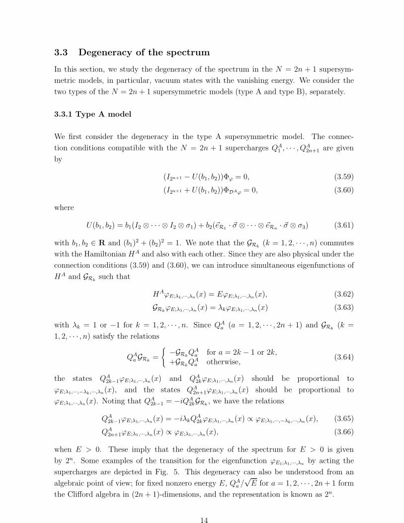
when E > 0. These imply that the degeneracy of the spectrum for E > 0 is given

by 2n. Some examples of the transition for the eigenfunction ϕE1;λ1,···,λn by acting the

supercharges are depicted in Fig. 5. This degeneracy can also be understood from an

algebraic point of view; for fixed nonzero energy E, QAa /

√E for a = 1, 2, · · · , 2n+ 1 form

the Clifford algebra in (2n+ 1)-dimensions, and the representation is known as 2n.

14

... ...

E

E1

Q2 +1nA

; λ ...λϕ

E n1 1

Q Q,2 1k 2 kA A

–

; λ ...λϕ

E n–1 1

Q Q21 ,

A A

; λ ... λλ ...ϕ

E nk–11

Q Q,2 1n 2 nA A

–

; λ ... λλ ...ϕ

E nk11 –

Figure 5: Examples of the transition for the eigenfunction ϕE1;λ1,···,λn under the action ofthe supercharges (QA

1 , · · · , QA2n+1)

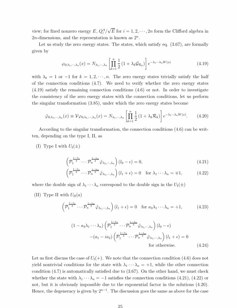
The above argument cannot apply for the case of E = 0. This is because any state

ϕ0(x) with vanishing energy must satisfy QAa ϕ0(x) = 0 for a = 1, 2, · · · , 2n + 1. The

equations QAa ϕ0(x) = 0 are equivalent to

DAϕ0(x) = 0. (3.67)

The above equation is easily solved, and we have formal solutions as

ϕ0;λ1,···,λn(x) = Nλ1,···,λn

[n∏

k=1

1

2(1 + λkGRk

)

]

e−λ1···λnW (x). (3.68)

Here, Nλ1,···,λn denotes normalization constants. By noting the Hamiltonian HA includes

only W ′(x) (but not W (x) itself), we have an ambiguity to choose W (x) to satisfy

PkW (x)Pk = W (x), k = 1, 2, · · · , n, (3.69)

Pn+1W (x)Pn+1 = −W (x). (3.70)

For a noncompact space, any non-normalizable states would be removed from the func-

tional space. The space is, however, compact in our model, so that these solutions are

always normalizable. Nevertheless, some of them must be removed from the functional

space. This is because some solutions are incompatible with the connection conditions.

Although the zero energy states trivially satisfy the half of the connection conditions

(3.60), we need to verify whether the states (3.68) satisfy the remaining connection con-

dition (3.59) or not.

In order to investigate the consistency of the zero energy states with the connection

conditions, we use the transformation (2.8), (2.9). This transformation yields

U(b1, b2) ≡ V U(b1, b2)V† = b1 (I2 ⊗ · · · ⊗ I2 ⊗ σ1) + b2 (σ3 ⊗ · · · ⊗ σ3) , (3.71)

where

V ≡(

ei~v1·~σ ⊗ ei~v2·~σ ⊗ · · · ⊗ ei~vn·~σ ⊗ I2)

, ei~vk ·~σ ∈ SU(2). (3.72)

15

The transformation is a singular unitary transformation because it, in general, changes

connection conditions of wavefunctions at singular points. The transformation may be

regarded as a duality connecting different theories (with different connection conditions).

Moreover, the transformation gives us the convenient expression for the connection con-

dition.

For instance, we consider the model which possesses two point singularities placed at

x = 0, l (n = 1) as an example. The connection condition (3.59) is transformed by (3.72)

to

(I4 − U(b1, b2))Φϕ = 0, (3.73)

where

U(b1, b2) = b1(I2 ⊗ σ1) + b2(σ3 ⊗ σ3), ϕ = V1ϕ, V1 = ei~v1·~P1. (3.74)

Explicitly, eq. (3.73) is written as

1− b2 −b1 0 0−b1 1 + b2 0 00 0 1 + b2 −b10 0 −b1 1− b2

ϕ(l − ǫ)ϕ(0 + ǫ)ϕ(−l + ǫ)ϕ(−0 − ǫ)

= 0. (3.75)

We observe that the above connection condition is separated into two independent condi-

tions, depending on the argument of the wavefunction. This suggests that it is useful to

assign the eigenvalue λ1 of the operator R1 for the wavefunction. To this end, we define

the projection operator,1

2(1 + λ1R1) . (3.76)

By multiplying (1 + λ1R1)/2 from the left to eq. (3.73), we obtain the boundary vector

as

Φ( 1+λ1R12 )ϕ =

ϕλ1=+1(l − ǫ) = 0ϕλ1=+1(0 + ǫ) = 0

00

for λ1 = +1,

00

ϕλ1=−1(−l + ǫ) = 0ϕλ1=−1(0− ǫ) = 0

for λ1 = −1.

(3.77)

Then, the connection conditions (3.73) are reduced to

• for b2 = 1 (and b1 = 0)

ϕλ1=+1(0 + ǫ) = 0, (3.78)

ϕλ1=−1(−l + ǫ) = 0, (3.79)

16

• for b2 6= 1

(1− b2)ϕλ1=+1(l − ǫ)− b1ϕλ1=+1(0 + ǫ) = 0, (3.80)

(1− b2)ϕλ1=−1(0− ǫ)− b1ϕλ1=−1(−l + ǫ) = 0. (3.81)

Let us also note that the Schrodinger equations can be written separately in each region

of (0 < x < l) and (−l < x < 0),

Hϕλ1=+1(x) = Eϕλ1=+1(x) (0 < x < l) with (3.78) or (3.80), (3.82)

Hϕλ1=−1(x) = Eϕλ1=−1(x) (−l < x < 0) with (3.79) or (3.81), (3.83)

where H ≡ VHV†.

Similarly, we can generalize the above argument to the case of n. The connection

conditions (3.59) can be written as

(I2n+1 − U(b1, b2))Φ(∏n

k=1

1+λkRk2

)

ϕ= 0 (3.84)

where

ϕ ≡ Vϕ with V ≡ V1V2 · · · Vn, Vi = ei~vi·~Pi. (3.85)

In this basis, the boundary vector can simply be written as

Φ(∏n

k=1

1+λkRk2

)

ϕ= Φϕλ1,···,λn

=

0...0

(

P1−λ1

21 · · · P

1−λn2

n ϕλ1,···,λn

)

(l0 − ǫ)(

P1−λ1

21 · · · P

1−λn2

n ϕλ1,···,λn

)

(l1 + ǫ)

0...0

. (3.86)

The connection conditions (3.84) are reduced to

• for b2 = 1 (and b1 = 0)

(

P1−λ1

21 · · · P

1−λn2

n ϕλ1,···,λn

)

(l0 − ǫ) = 0 for λ1 · · ·λn = −1, (3.87)(

P1−λ1

21 · · · P

1−λn2

n ϕλ1,···,λn

)

(l1 + ǫ) = 0 for λ1 · · ·λn = +1, (3.88)

• for b2 6= 1

17

(1− b2)(

P1−λ1

21 · · · P

1−λn2

n ϕλ1,···,λn

)

(l0 − ǫ)− b1

(

P1−λ1

21 · · · P

1−λn2

n ϕλ1,···,λn

)

(l1 + ǫ) = 0

for λ1 · · ·λn = +1, (3.89)

(1− b2)(

P1−λ1

21 · · · P

1−λn2

n ϕλ1,···,λn

)

(l1 + ǫ)− b1

(

P1−λ1

21 · · · P

1−λn2

n ϕλ1,···,λn

)

(l0 − ǫ) = 0

for λ1 · · ·λn = −1. (3.90)

The Schrodinger equations can be separated into 2n regions of (ls < x < ls+1) (s =

0, 1, · · · , 2n − 1).

Now, we are ready to discuss whether the zero energy states satisfy the connection

conditions or not. With the transformations (3.85), the zero energy states (3.68) become

ϕ0;λ1,···,λn(x) ≡ Vϕ0;λ1,···,λn(x) = Nλ1,···,λn

[n∏

k=1

1

2(1 + λkRk)

]

e−λ1···λnW (x). (3.91)

The states (3.91) do not satisfy the connection conditions (3.87), (3.88) for b2 = 1. Al-

though for general W (x), the connection conditions (3.89), (3.90) are not satisfied by the

zero energy states for b2 6= 1, there is, however, an exceptional case, where W (x) satisfies√

1− b11 + b1

= e2W (l0−ǫ). (3.92)

With this special W (x), all the states (3.91) become supersymmetric vacuum states com-

patible with the connection conditions.

There is no supersymmetric vacuum state for general W (x). Therefore, the supersym-

metry is “spontaneously”5 broken. While, for the special W (x) satisfying (3.92), we have

the supersymmetric vacuum states, and the degeneracy is 2n.

Let us note that the Pn+1 becomes physical when b2 = 0 and commutes with the

Hamiltonian HA only for W ′′(x) = 0. We can introduce the simultaneous eigenfunctions

of the Hamiltonian HA, GRk(k = 1, 2, · · · , n) and Pn+1,

HAϕE;λ1,···,λn,λn+1(x) = EϕE;λ1,···,λn,λn+1(x), (3.93)

GRkϕE;λ1,···,λn,λn+1(x) = λkϕE;λ1,···,λn,λn+1(x), (3.94)

Pn+1ϕE;λ1,···,λn,λn+1(x) = λn+1ϕE;λ1,···,λn,λn+1(x). (3.95)

The new label λn+1 on the wavefunction suggests the enhancement of the degeneracy

for the state with E > 0. In order to confirm it, let us define new operator QAa (a =

1, 2, · · · , 2n+ 1) as

QAa ≡ i

2Γa

(

R1 · · ·Rn+1d

dx

)

. (3.96)

Then, the Hamiltonian HA can be written as

HA = 2(QAa )

2 = 2(QAa )

2 +1

2c2, (3.97)

5If there is no zero energy state, we say that supersymmetry is spontaneously broken by analogy withsupersymmetric quantum field theory. Other mechanisms of (spontaneous) supersymmetry breaking dueto boundary effects have been found in Refs. [17, 18].

18

where c2 ≡ (W ′(x))2 is independent of x for W ′′(x) = 0. The energy is bounded from

below as

E ≥ 1

2c2. (3.98)

We can show that QAa (a = 1, 2, · · · , 2n+1) is physical under the connection conditions

(3.59) and (3.60). Since QAa and GRk

(k = 1, 2, · · · , n), Pn+1 satisfy

Pn+1QAa = −QA

aPn+1 for a = 1, 2, · · · , 2n+ 1. (3.99)

GRkQAa =

{

−QAa GRk

for a = 2k − 1, 2k,

+QAa GRk

otherwise(3.100)

and QA2k−1 = −iQA


QA2k−1ϕE;λ1,···,λn,λn+1 = −iλkQA

2kϕE;λ1,···,λn,λn+1 ∝ ϕE;λ1,···,−λk,···,λn,−λn+1, (3.101)

QA2n+1ϕE;λ1,···,λn,λn+1 ∝ ϕE;λ1,···,λn,−λn+1. (3.102)

Thus, in this case, the degeneracy for E > 12c2 is given by 2n+1. This result can also be

obtained from an algebraic point of view; QAa /

√E (a = 1, 2, · · · , 2n + 1) and Pn+1 form

the Clifford algebra in (2n+ 2)- dimensions and the representation is known as 2n+1.

Let us discuss the case of E = 12c2. The state with E = 1

2c2 satisfies QA

a ϕE= 12c2(x) =

0 (a = 1, 2, · · · , 2n+ 1), which is equivalent to

d

dxϕE= 1

2c2;λ1,···,λn,λn+1

(x) = 0, (3.103)

where we have performed the singular transformation (3.85). The solution satisfying

(3.103) always have only λn+1 = 1 state because the state with λn+1 = −1 have disconti-

nuity except for the original singularities. The formal solutions for the state with E = 12c2

are given by

ϕE= 12c2;λ1,···,λn,λn+1=+1 = Nλ1,···,λn,λn+1=+1

[n∏

k=1

1

2(1 + λkRk)

]

. (3.104)

Let us note that the solution (3.104) shows that it takes constant values between the two

neighboring singularities.

Let us study the compatibility of the solutions (3.104) with the connection conditions

(3.87)-(3.90). For b1 = +1, all the states with E = 12c2 satisfy the connection conditions

(3.89) and (3.90), so that the degeneracy is 2n, while for b1 = −1, all the states do not

satisfy the connection conditions (3.89), (3.90) and are removed from the functional space.

We can introduce the “fermion” number operator as

(−1)F ≡ Pn+1 (3.105)

for b2 = 0 and W ′(x) = 0 (c = 0). We note that W ′(x) = 0 ensures6

{QAa , (−1)F} = 0. (3.106)

6Let us note that when W ′′(x) = 0, Pn+1 anticommutes with QAa . If we regard QA

a as a supercharge,Pn+1 can be taken as the “fermion” number operator.

19

We call states with (−1)F = +1(−1) “bosonic” (“fermionic”) ones. Under the relation

(3.106), QAa ϕE;λ1,···,λn(x) have the opposite eigenvalues of (−1)F as ϕE;λ1,···,λn(x).

We discuss the Witten index in this model. The Witten index of an operator O with

O2 = 1 is defined by

∆W ;O ≡ NE=0+ −NE=0

− , (3.107)

where NE=0± denotes the number of the zero energy states with O = ±1, respectively and

all the nonzero energy states between O = 1 and O = −1 are degenerate.

The Witten index of Pn+1 for W ′(x) = 0 (c = 0)7 and b2 = 0 is given by

∆W ;Pn+1 = 2n. (3.108)

When W ′′(x) = 0, the zero energy states do not exist. However, by shifting the energy,

E → E = E − 12c2, there is a nonzero Witten index for E = 0 (E = 1

2c2),

∆W ;Pn+1 = N E=0+ −N E=0

− = 2n. (3.109)

We should make a comment on the special case (3.92) in which the zero energy states

exist. In this case, the Witten index of GR1 · · · GRnvanishes because NE=0

+ and NE=0− are

the same,

NE=0GR1

···GRn=+1 = NE=0GR1

···GRn=−1 = 2n−1. (3.110)

3.3.2 Type B model

The connection conditions compatible with the N = 2n + 1 supercharges QB1 , · · · , QB

2n+1

are given by

(I2n+1 − U(b1, b2))Φϕ = 0, (3.111)

(I2n+1 + U(b1, b2))ΦDBϕ = 0, (3.112)

where

U(b1, b2) = b1(I2 ⊗ · · · ⊗ I2 ⊗ σ1) + b2(~eR1 · ~σ ⊗ · · · ⊗ ~eRn· ~σ ⊗ σ3) (3.113)

with b1, b2 ∈ R and (b1)2 + (b2)

2 = 1. We first note that the GRk(k = 1, 2, · · · , n)

commute with HB and also with each other. Since they are also physical under the

connection conditions (3.111), (3.112), we can introduce simultaneous eigenfunctions,

HBϕE;λ1,···,λn(x) = EϕE;λ1,···,λn(x), (3.114)

GRkϕE;λ1,···,λn(x) = λkϕE;λ1,···,λn(x) (3.115)

7In this case, QAa is the same as QA

a .

20

with λk = 1 or λk = −1 for k = 1, 2, · · · , n. The supercharges QBa (a = 1, 2, · · · , 2n + 1)

and GRk(k = 1, 2, · · · , n) satisfy the relations

QBa GRk

=

{

−GRkQBa for a = 2k − 1, 2k,

+GRkQBa otherwise.

(3.116)

Noting that QB2k−1 = −iQB


QB2k−1ϕE;λ1,···,λn(x) = −iλkQB

2kϕE;λ1,···,λn(x) ∝ ϕE;λ1,···,−λk,···,λn(x), (3.117)

QB2n+1ϕE;λ1,···,λn(x) ∝ ϕE;λ1,···,λn(x), (3.118)

then the degeneracy of the spectrum is given by 2n for E > 0. This result can also be

obtained from an algebraic point of view, that is, for fixed nonzero energy E, QBa /

√E for

a = 1, 2, · · · , 2n+ 1 form Clifford algebra in (2n + 1)-dimensions, and the representation

is known as 2n.

The above argument cannot apply for E = 0 states because QBa ϕ0 = 0. The equations

QBa ϕ0(x) = 0 are easily solved and we have formal solutions as

ϕ0;λ1,···,λn(x) = Nλ1,···,λn

[n∏

k=1

1

2(1 + λkGRk

)

]

eV (x), (3.119)

where Nλ1,···,λn denotes normalization constants. Since the Hamiltonian HB includes only

V ′(x) (but not V (x) itself), we have an ambiguity to choose V (x) to satisfy

PiV (x)Pi = V (x), i = 1, 2, · · · , n+ 1. (3.120)

Under the singular unitary transformation (3.85), the zero energy states become


[n∏

k=1

1

2(1 + λkRk)

]

eV (x). (3.121)

The zero energy states trivially satisfy the half of the connection conditions (3.112). Let us

discuss the remaining connection conditions (3.111), which are given by eqs. (3.87)-(3.90).

The states (3.121) do not satisfy the connection conditions (3.87), (3.88). On the

other hand, the connection conditions (3.89), (3.90) are neither satisfied by the zero

energy states. There is, however, an exceptional case

b1 = 1. (3.122)

This is because V (l0 − ǫ) = V (l1 + ǫ).

The Pn+1 commutes with GRk(k = 1, 2, · · · , n), HB and becomes physical only for

b2 = 0. An accidental degeneracy occurs in this case. We can introduce simultaneous

eigenfunctions of the Hamiltonian HB, GRk(k = 1, 2, · · · , n) and Pn+1 such that

HBϕE;λ1,···,λn,λn+1(x) = EϕE;λ1,···,λn,λn+1(x), (3.123)

GRkϕE;λ1,···,λn,λn+1(x) = λkϕE;λ1,···,λn,λn+1(x), (3.124)

Pn+1ϕE;λ1,···,λn,λn+1(x) = λn+1ϕE;λ1,···,λn,λn+1(x). (3.125)

21

The QBa and Pn+1 satisfy the relations

QBa Pn+1 = −Pn+1Q

Ba , a = 1, 2, · · · , 2n+ 1. (3.126)

Eqs. (3.116), (3.117) and (3.126) imply that the degeneracy of the spectrum for E > 0 is

given by 2n+1.

The zero energy formal solutions are

ϕ0;λ1,···,λn,λn+1=+1(x) = Nλ1,···,λn

[n∏

k=1

1

2(1 + λkGRk

)

]

eV (x). (3.127)

Here ϕ0;λ1,···,λn,λn+1=−1(x) do not exist because the states cannot construct without new

singularities except for the original singular points x = ls (s = 0, 1, · · · , 2n−1). For b1 = 1,

all the zero energy states (3.127) become supersymmetric vacuum states compatible with

the connection conditions (3.89), (3.90), while, for b1 = −1, all the states are incompatible

with the connection conditions (3.89), (3.90).

The Pn+1 can be regarded as the “fermion” number operator only if b2 = 0,

(−1)F = Pn+1. (3.128)

The operator satisfies

{QBa , (−1)F} = 0. (3.129)

There is a nonzero Witten index of Pn+1 only for b1 = 1 and b2 = 0,

∆W ;Pn+1 = 2n. (3.130)

4 Reduction of the supersymmetry

4.1 General discussion

In this section, we provide a general discussion on a reduction of the supersymmetry by

relaxing the connection conditions8. So far, we have considered the connection conditions

compatible with all the 2n + 1 supercharges. Here we require that only a subset of the

supercharges are physical. To put it the other way around, we allow some of the 2n + 1

supercharges to become incompatible with connection conditions.

Let us consider the m supercharges that are a subset of the 2n+ 1 supercharges (3.1)

((3.2)). The connection conditions compatible with the m supercharges are given by

(I2n+1 − U) Φϕ = 0, (4.1)

(I2n+1 + U) ΦDA(B)ϕ = 0, (4.2)

8Falomir and Pisani have also discussed the reduction of supersymmetry in the presence of singularsuperpotentials[19].

22

where the constraints on the characteristic matrix U are

U †U = I2n+1 , (4.3)

U2 = I2n+1 , (4.4)

γiUγi = −U. (4.5)

Here the number of γi is m, which is a subset of the γa (a = 1, 2, · · · , 2n + 1). The

difference from the case of the N = 2n + 1 supersymmetry is in eq. (4.5), that is, the

number of γi is smaller than that of the case of the N = 2n + 1 supersymmetry. The

smaller the number of γi in eq. (4.5) becomes, the larger the number of parameters of

the characteristic matrix U becomes. This implies that the supercharges not belonging

to the subset are not the physical operators.

4.2 N = 2n supersymmetry

In this section, we consider some N = 2n supersymmetric models as examples of the

reduced supersymmetry. We choose 2n supercharges that are subset of the 2n+ 1 super-

charges (3.1), (3.2) as

(a) QA1 , Q

A2 , · · · , QA

2n, (b) QA1 , Q

A2 , · · · , QA

2n−1, QA2n+1,

(c) QB1 , Q

B2 , · · · , QB

2n, (d) QB1 , Q

B2 , · · · , QB

2n−1, QB2n+1.

We will obtain the connection conditions compatible with the constraints (4.3)-(4.5) and

study the degeneracy of the spectrum and the zero energy states in each model.

4.2.1 (a) QA1 , Q

A2 , · · · , QA

2n

In order for the supercharges QA1 , · · · , QA

2n to satisfy the superalgebra, we need

only eq. (3.8). And the Hamiltonian is also given by eq. (3.14). The N = 2n

supersymmetry has already been found and discussed in Ref. [12]. The results of the

connection conditions and degeneracy of the spectrum in this subsection agree with those

in Ref. [12] although the analysis has been incomplete in Ref. [12].

The connection conditions compatible with the 2n supercharges QA1 , · · · , QA

2n are

(I2n+1 − U)Φϕ = 0, (4.6)

(I2n+1 + U)ΦDAϕ = 0, (4.7)

where

U2 = I2n+1 , (4.8)

U †U = I2n+1 , (4.9)

γiUγi = −U, i = 1, 2, · · · , 2n. (4.10)

23

In order to obtain the expression of the characteristic matrix U , we use the expansion

(3.48)-(3.50). Eq. (4.10) implies that the nonvanishing coefficients are only four,

a1 ≡ Cα1=0,α2=0,···,αn=0,αn+1=1, a2 ≡ Cα1=0,α2=0,···,αn=0,αn+1=2, (4.11)

a3 ≡ Cα1=3,α2=3,···,αn=3,αn+1=3, a4 ≡ Cα1=3,α2=3,···,αn=3,αn+1=0. (4.12)

Thus, the characteristic matrix U can be expanded as

U = a1 (I2 ⊗ · · · ⊗ I2 ⊗ σ1) + a2 (I2 ⊗ · · · ⊗ I2 ⊗ σ2)

+a3 (~eR1 · ~σ ⊗ · · · ⊗ ~eRn· ~σ ⊗ σ3) + a4 (~eR1 · ~σ ⊗ · · · ⊗ ~eRn

· ~σ ⊗ I2) . (4.13)

Let us note the number of parameters in the characteristic matrix U is larger than that

in the N = 2n+1 supersymmetric model because of the decrease of the conditions on the

U . We further restrict the form of U by imposing the conditions (4.8) and (4.9). Then,

we obtain that

(a4)2 = 1 and a1 = a2 = a3 = 0, (4.14)

or

(a1)2 + (a2)

2 + (a3)2 = 1 and a4 = 0 (4.15)

with a1, a2, a3, a4 ∈ R. Thus, the characteristic matrix U compatible with the 2n super-

symmetry is given by

(I) Type I

UI(±) = ± (~eR1 · ~σ ⊗ · · · ⊗ ~eRn· ~σ ⊗ I2) , (4.16)

(II) Type II

UII(a) = a1 (I2 ⊗ · · · ⊗ I2 ⊗ σ1) + a2 (I2 ⊗ · · · ⊗ I2 ⊗ σ2)

+a3 (~eR1 · ~σ ⊗ · · · ⊗ ~eRn· ~σ ⊗ σ3) (4.17)

with (a1)2 + (a2)

2 + (a3)2 = 1.

Let us next study the degeneracy of the spectrum. We note that GRk(k = 1, 2, · · · , n)

commutes with the Hamiltonian HA and is physical under the connection conditions

(4.16), (4.17), so that the state with E(> 0) is labeled by the quantum number λk, which

is the eigenvalue of GRk. Noting that QA

2k−1 = −iQA2kGRk

and the relations

QAi GRk

=

{

−GRkQAi for i = 2k − 1 or 2k,

+GRkQAi otherwise

(4.18)

for k = 1, 2, · · · , n, we have the relations (3.65) for k = 1, 2, · · · , n. Thus, the degeneracy

for E > 0 is given by 2n. This result can also be obtained from an algebraic point of

24

view; for fixed nonzero energy E, QAi /

√E for i = 1, 2, · · · , 2n form the Clifford algebra in

2n-dimensions, and the representation is known as 2n.

Let us study the zero energy states. The states, which satisfy eq. (3.67), are formally

given by

ϕ0;λ1,···,λn(x) = Nλ1,···,λn

[n∏

k=1

1

2(1 + λkGRk

)

]

e−λ1···λnW (x) (4.19)

with λk = 1 or −1 for k = 1, 2, · · · , n. The zero energy states trivially satisfy the half

of the connection conditions (4.7). We need to verify whether the zero energy states

(4.19) satisfy the remaining connection conditions (4.6) or not. In order to investigate

the consistency of the zero energy states with the connection conditions, let us perform

the singular transformation (3.85), under which the zero energy states become


[n∏

k=1

1

2(1 + λkRk)

]

e−λ1···λnW (x). (4.20)

According to the singular transformation, the connection conditions (4.6) can be writ-

ten, depending on the type I, II, as

(I) Type I with UI(±)

(

P1−λ1

21 · · · P

1−λn2

n ϕλ1,···,λn

)

(l0 − ǫ) = 0, (4.21)(

P1−λ1

21 · · · P

1−λn2

n ϕλ1,···,λn

)

(l1 + ǫ) = 0 for λ1 · · ·λn = ∓1, (4.22)

where the double sign of λ1 · · ·λn correspond to the double sign in the UI(±)

(II) Type II with UII(a)

(

P1−λ1

21 · · · P

1−λn2

n ϕλ1,···,λn

)

(l1 + ǫ) = 0 for a3λ1 · · ·λn = +1, (4.23)

(1− a3λ1 · · ·λn)(

P1−λ1

21 · · · P

1−λn2

n ϕλ1,···,λn

)

(l0 − ǫ)

−(a1 − ia2)(

P1−λ1

21 · · ·P

1−λn2

n ϕλ1,···,λn

)

(l1 + ǫ) = 0

for otherwise. (4.24)

Let us first discuss the case of UI(+). We note that the connection condition (4.6) does not

yield nontrivial conditions for the state with λ1 · · ·λn = +1, while the other connection

condition (4.7) is automatically satisfied due to (3.67). On the other hand, we must check

whether the state with λ1 · · ·λn = −1 satisfies the connection conditions (4.21), (4.22) or

not, but it is obviously impossible due to the exponential factor in the solutions (4.20).

Hence, the degeneracy is given by 2n−1. The discussion goes the same as above for the case

25

of UI(−), so that the degeneracy is, again, 2n−1. Thus, the supersymmetry is unbroken.

We have seen that once we determine the connection condition UI(±), the states with

λ1 · · ·λn = ±1 can satisfy the connection conditions.

For the type II connection conditions, the zero energy states (4.20) are found to be

inconsistent with the connection conditions (4.23), (4.24), so that there are no vacuum

states with zero energy. There is, however, an exception. If the following relations are

satisfied√

1− a31 + a3

= eW (l0−ǫ)−W (l1+ǫ), a1 =√

1− (a3)2, a2 = 0, (4.25)

all the states (4.20) accidentally become supersymmetric vacuum states compatible with

the connection conditions (4.24), hence, the degeneracy is 2n. Therefore, for the type II

connection conditions, supersymmetry is spontaneously broken except for the above case.

If a2 = 0, the supercharge QA2n+1 become physical. Then, QA

1 , · · · , QA2n+1 form the

N = 2n+1 superalgebra if we require the conditions (3.9). Therefore, the supersymmetry

is enhanced to the N = 2n + 1 supersymmetry, and the degeneracy has been studied in

the previous section.

We can introduce the “fermion” number operator as

(−1)F ≡ GR1 · · · GRn, (4.26)

which is physical under the connection conditions (4.6) and (4.7), and commutes (anti-

commutes) with the Hamiltonian HA (all the supercharges QAi (i = 1, 2, · · · , 2n)). Let

us note that eigenvalues of the fermion number operator are λ1 · · ·λn = ±1. The Witten

index of GR1 · · · GRnwith UI(±) is given by

∆W ;GR1···GRn

= ±2n−1, (4.27)

where the double sign correspond to the double sign in the UI(±).

If W ′(x) = 0, the Pn+1 is physical under the connection condition (4.16). And it

(anti)commutes with the (supercharges) HA. Then, we can introduce the Witten index

of Pn+1,

∆W ;Pn+1 = 2n−1. (4.28)

For the type II connection conditions with UII(a), the Witten index of GR1 · · · GRn

vanishes because there are no zero energy states. We should make a comment on the

special case (4.25), in which the zero energy states exist. The Witten index of GR1 · · · GRn

is, however, zero because NE=0+ and NE=0

− are the same,

NE=0GR1

···GRn=+1 = NE=0GR1

···GRn=−1 = 2n−1. (4.29)

26

4.2.2 (b) QA1 , Q

A2 , · · · , QA

2n−1, QA2n+1

The N = 2n supercharges QA1 , Q

A2 , · · · , QA

2n−1, QA2n+1 form the N = 2n superalge-

bra if the function W ′(x) obeys (3.8) and (3.9). The constraints on the characteristic

matrix U are

U2 = I2n+1 , (4.30)

U †U = I2n+1 , (4.31)

γiUγi = −U, i = 1, 2, · · · , 2n− 1, 2n+ 1. (4.32)

We expand the U in the expression (3.48)-(3.50). Because of the conditions (4.32), nonzero

coefficients are only four,

a1 ≡ Cα1=0,α2=0,···,αn=0,αn+1=1, a2 ≡ Cα1=3,α2=3,···,αn−1=3,αn=2,αn+1=3,a3 ≡ Cα1=3,α2=3,···,αn=3,αn+1=3, a4 ≡ Cα1=0,α2=0,···,αn−1=0,αn=1,αn+1=1.

(4.33)

The conditions (4.30) and (4.31) imply that

(a4)2 = 1 and a1 = a2 = a3 = 0, (4.34)

or

(a1)2 + (a2)

2 + (a3)2 = 1 and a4 = 0 (4.35)

with a1, a2, a3, a4 ∈ R. Thus, the characteristic matrix U compatible with the 2n super-

charges QA1 , · · · , QA

2n−1, QA2n+1 are

(I) Type I

UI(±) = ± (I2 ⊗ · · · ⊗ I2 ⊗ ~ePn· ~σ ⊗ σ1) , (4.36)

(II) Type II

UII(a) = a1 (I2 ⊗ · · · ⊗ I2 ⊗ σ1)

+a2(

~eR1 · ~σ ⊗ · · · ⊗ ~eRn−1 · ~σ ⊗ ~eQn· ~σ ⊗ σ3

)

+a3 (~eR1 · ~σ ⊗ · · · ⊗ ~eRn· ~σ ⊗ σ3) (4.37)

with (a1)2 + (a2)

2 + (a3)2 = 1. With the above characteristic matrix U , the connection

conditions are given by

(I2n+1 − U)Φϕ = 0, (4.38)

(I2n+1 + U)ΦDAϕ = 0. (4.39)

In this case, GRnis no longer physical under the connection conditions (4.36), (4.37),

but instead, GPnPn+1 is physical. The Hamiltonian HA, GRk

(k = 1, 2, · · · , n − 1) and

27

GPnPn+1 are physical, and they commute with each other. We can introduce simultaneous

eigenfunctions of these operators such that

HAϕE;λ1,···,λ′n(x) = EϕE;λ1,···,λ′n(x), (4.40)

GRkϕE;λ1,···,λ′n(x) = λkϕE;λ1,···,λ′n(x), k = 1, 2, · · · , n− 1, (4.41)

(GPnPn+1)ϕE;λ1,···,λ′n(x) = λ′nϕE;λ1,···,λ′n(x) (4.42)

with λk = 1 or −1 for k = 1, 2, · · · , n − 1 and λ′n = 1 or −1. In this case, we have the

relations

QA2k−1ϕE;λ1,···,λ′n(x) = −iλkQA

2kϕE;λ1,···,λ′n(x) ∝ ϕE;λ1,···,−λk,···,λ′n(x),

k = 1, 2, · · · , n− 1, (4.43)

QA2n−1ϕE;λ1,···,λ′n(x) ∝ ϕE;λ1,···,−λ′n(x), (4.44)

QA2n+1ϕE;λ1,···,λ′n(x) ∝ ϕE;λ1,···,−λ′n(x), (4.45)

because

GRkQAi =

{

−QAi GRk

for k = 2i− 1, 2i,+QA

i GRkotherwise,

(4.46)

(GPnPn+1)Q

Ai = −QA

i (GPnPn+1) (4.47)

for i = 1, 2, · · · , 2n− 1, 2n + 1 and QA2k−1 = −iQA

2kGRkfor k = 1, 2, · · · , n − 1. Thus, the

degeneracy for E > 0 is given by 2n. This result can also be obtained from an algebraic

point of view; for fixed nonzero energy E, QAi /

√E for i = 1, 2, · · · , 2n − 1, 2n + 1 form

the Clifford algebra in 2n-dimensions, and the representation is known as 2n.

The above argument cannot apply for the zero energy states. The zero energy states

are given by solving

DAϕ0(x) =

[(

R1 · · ·Rn+1d

dx

)

+ λ1 · · ·λn−1GRn(R1 · · ·Rn+1W

′(x))

]

ϕ0;λ1,···,λ′n(x) = 0.

(4.48)

The solutions to eq. (4.48) are formally given by

ϕ0;λ1,···,λ′n(x) = Nλ1,···,λ′n

(n−1∏

k=1

1 + λkGRk

2

)

×{(

1 + GRn

2

)

e−λ1···λn−1W (x) + λ′n

(1− GRn

2

)

eλ1···λn−1W (x)}

,(4.49)

and trivially satisfy the half of the connection conditions (4.39). We need to verify whether

the zero energy states satisfy the remaining connection conditions (4.38) or not. Under

the singular unitary transformation (3.85), the zero energy states become

ϕ0;λ1,···,λ′n(x) ≡ Vϕ0;λ1,···,λ′n(x)

= Nλ1,···,λ′n

(n−1∏

k=1

1 + λkRk

2

)

×{(

1 +Rn

2

)

e−λ1···λn−1W (x) + λ′n

(1−Rn

2

)

eλ1···λn−1W (x)}

,(4.50)

28

and accordingly the connection conditions, (4.38) can be written as

(I) Type I with UI(±)

(

P1−λ1

21 · · · P

1−λn−12

n−1 ϕλ1,···,λ′n

)

(l0 − ǫ) = 0, (4.51)

(

P1−λ1

21 · · · P

1−λn−12

n−1 ϕλ1,···,λ′n

)

(l1 + ǫ) = 0 for λ′n = ∓1, (4.52)

where the double sign of λ′n correspond to the double sign in the UI(±),

(II) Type II with UII(a)

(

P1−λ1

21 · · · P

1−λn−12

n−1 ϕλ1,···,λ′n

)

(l1 + ǫ) = 0 for a3λ1 · · ·λn−1 = +1, (4.53)

(1− a3λ1 · · ·λn−1)

(

P1−λ1

21 · · · P

1−λn−12

n−1 ϕλ1,···,λ′n

)

(l0 − ǫ)

−(a1 − ia2λ1 · · ·λ′n)(

P1−λ1

21 · · · P

1−λn−12

n−1 ϕλ1,···,λ′n

)

(l1 + ǫ) = 0

for otherwise. (4.54)

We first consider the case of UI(+) (UI(−)). The zero energy states with λ′n =

+1 (λ′n = −1) can satisfy the connection conditions (4.38), (4.39) because the connection

conditions (4.38) do not yield nontrivial conditions for the states with λ′n = +1 (λ′n = −1),

and the connection conditions (4.39) are automatically satisfied due to (4.48). On the

other hand, the states with λ′n = −1 (λ′n = +1) do not satisfy the connection conditions

(4.51), (4.52) because of the exponential factor in the solution. Thus, the degeneracy of

the zero energy states for the case of UI(±) is given by 2n−1, and the supersymmetry is

unbroken.

For the case of UII(a), the zero energy states do not satisfy the connection conditions

(4.53), (4.54) with one exception. If the following relations are satisfied

√

1− a31 + a3

= e2W (l0−ǫ), a1 =√

1− (a3)2, a2 = 0, (4.55)

all the states (4.50) are compatible with the connection conditions (4.54), then, the de-

generacy is 2n. Hence, for the type II connection conditions, the supersymmetry is spon-

taneously broken except for the above case.

Note that if a2 = 0, the supercharge QA2n becomes physical. Then, the supersymmetry

is enhanced to the N = 2n+ 1 supersymmetry.

In this model, GPnPn+1 can be regarded as the “fermion” number operator,

(−1)F = GPnPn+1. (4.56)

29

The Witten indices of GPnPn+1, Pn+1 for UI(±) are given by

∆W ;GPnPn+1 = ±2n−1, (4.57)

∆W ;Pn+1 = 2n−1, only for W ′(x) = 0, (4.58)

where the double sign in eq. (4.57) correspond to the double sign in the UI(±). For

UII(a), the Witten index of GPnPn+1 vanishes because the zero energy states do not exist.

Let us comment on the special case (4.55), where we have the zero energy states. We

note that the supersymmetry is enhanced to the same N = 2n+ 1 supersymmetry in the

special case (4.55) as that in the previous section.

4.2.3 (c) QB1 , · · · , QB

2n

The N = 2n supercharges QB1 , · · · , QB

2n form the N = 2n superalgebra if the V ′(x) obeys

(3.10). In this case, the constraints on the characteristic matrix U are same with the

case of (a). The connection conditions are given by

(I2n+1 − U)Φϕ = 0, (4.59)

(I2n+1 + U)ΦDBϕ = 0, (4.60)

where U is given by (4.16) or (4.17).

For UI(±), the GRk(k = 1, 2, · · · , n) and Pn+1 are physical under the connection condi-

tions (4.59),(4.60) and commute with HB. We can introduce simultaneous eigenfunctions

of HB, GRk(k = 1, 2, · · · , n) and Pn+1 such that

HBϕE;λ1,···,λn+1(x) = EϕE;λ1,···,λn+1(x), (4.61)

GRkϕE;λ1,···,λn+1(x) = λkϕE;λ1,···,λn+1(x), k = 1, 2, · · · , n, (4.62)

Pn+1ϕE;λ1,···,λn+1(x) = λn+1ϕE;λ1,···,λn+1(x). (4.63)

Although the labels in ϕ increase, the degeneracy of the spectrum for E > 0 states does

not increase in this model. The QBi (i = 1, 2, · · · , 2n), GRk

(k = 1, 2, · · · , n) and Pn+1

satisfy

Pn+1QBi = −QB

i Pn+1 for i = 1, 2, · · · , 2n, (4.64)

GRkQBi =

{

−QBi GRk

for i = 2k − 1, 2k,+QB

i GRkotherwise,

(4.65)

The supercharge QBi (i = 1, 2, · · · , n) changes not only the sign of λi but also the sign of

λn+1, so that no supercharge connects λ1 · · ·λn+1 = +1 states with λ1 · · ·λn+1 = −1 ones.

Therefore, The degeneracy between the states with λ1 · · ·λn+1 = +1 and the states with

λ1 · · ·λn+1 = −1 is not guaranteed, so that the 2n+1-fold degeneracy is not ensured.

Since QB2k−1 = −iQB

2kGRkfor k = 1, 2, · · · , n and

QB2k−1ϕE;λ1,···,λn(x) = −iλkQB

2kϕE;λ1,···,λn(x) ∝ ϕE;λ1,···,−λk,···,−λn(x) (4.66)

30

for k = 1, 2, · · · , n, the 2n-fold degeneracy for E > 0 states is ensured. This result can

also be obtained from an algebraic point of view; for fixed nonzero energy E, QBi /

√E

for i = 1, 2, · · · , 2n form the Clifford algebra in 2n-dimensions, and the representation

is known as 2n. The Pn+1 is regarded as a “fermion” number operator (−1)F in the

type I connection conditions. For UII(a), since the Pn+1, in general, is not physical, the

degeneracy for E > 0 is 2n.

The zero energy states satisfying QBi ϕ0(x) = 0 are formally

ϕ0;λ1,···,λn(x) = Nλ1,···,λn

(n∏

k=1

1 + λkGRk

2

)

eV (x). (4.67)

The zero energy states trivially satisfy the half of the connection conditions (4.60). Under

the singular unitary transformation (3.85), the remaining connection conditions (4.59)

can be written by eqs. (4.21)-(4.24), and the zero energy states become


(n∏

k=1

1 + λkRk

2

)

eV (x). (4.68)

Let us first discuss the case of UI(+) (UI(−)). We note that the connection conditions

(4.59) do not yield nontrivial conditions for the states with λ1 · · ·λn = +1 (λ1 · · ·λn =

−1), while the other connection conditions (4.60) are automatically satisfied due to

DBϕ0(x) = 0. On the other hand, we must check whether the states with λ1 · · ·λn =

−1 (λ1 · · ·λn = +1) satisfy the connection conditions (4.21), (4.22) or not. It is obviously

impossible because of the exponential factor in the solution. Hence the degeneracy for

the zero energy states for the case of UI(±) is given by 2n−1, and the supersymmetry is

unbroken. We have seen that once we determine the connection conditions UI(±), the

state with λ1 · · ·λn = ±1 can satisfy the connection conditions.

For the type II connection conditions, the zero energy states (4.68) are found to be

inconsistent with the connection conditions (4.23), (4.24), so that there are no vacuum

states with zero energy. There is, however, an exception. If the following relation is

satisfied

a1 = 1, (4.69)


the connection conditions (4.24), then, the degeneracy is 2n. Hence, for the type II

connection conditions, supersymmetry is spontaneously broken except for the above case.

Note that if a2 = 0, the supercharge QB2n+1 becomes physical, therefore the supersymmetry

is enhanced to the N = 2n+1 supersymmetry, which is same as the type B model in the

previous section.

The fermion number operators can be defined as

(−1)F = GR1 · · · GRnfor UI(±) or UII(a), (4.70)

(−1)F = Pn+1 for UI(±) or UII(a1 = ±1). (4.71)

31

For UI(±), the Witten indices of GR1 · · · GRnand Pn+1 are given by

∆W ;GR1···GRn

= ±2n−1, (4.72)

∆W ;Pn+1 = 2n−1, (4.73)

where the double sign in eq. (4.72) correspond to the double sign in the UI(±). Let us

comment on the special case of UII(a) with a1 = 1, where we have the zero energy states.

We note that the supersymmetry is enhanced to the same N = 2n + 1 supersymmetry

even in the special case of a1 = 1 as that in the previous section.

4.2.4 (d) QB1 , · · · , QB

2n−1, QB2n+1

The N = 2n supercharges QB1 , · · · , QB

2n−1, QB2n+1 form the N = 2n superalgebra if

the V ′(x) are assumed to obey (3.10). The characteristic matrix U is again given by

(4.36),(4.37). The connection conditions become

(I2n+1 − U)Φϕ = 0, (4.74)

(I2n+1 + U)ΦDBϕ = 0. (4.75)

In this model, GRk(k = 1, 2, · · · , n − 1) and GPn

Pn+1 are physical and commute with

HB. Since these operators commute with each other, we can introduce simultaneous

eigenfunctions of HB, GRk(k = 1, 2, · · · , n− 1) and GPn

Pn+1 such that

HBϕE;λ1,···,λ′n(x) = EϕE;λ1,···,λ′n(x), (4.76)

GRkϕE;λ1,···,λ′n(x) = λkϕE;λ1,···,λ′n(x), k = 1, 2, · · · , n− 1, (4.77)

(GPnPn+1)ϕE;λ1,···,λ′n(x) = λ′nϕE;λ1,···,λ′n(x). (4.78)

Since

GRkQBi =

{

−QBi GRk

for k = 2i− 1, 2i,+QB

i GRkotherwise,

(4.79)

(GPnPn+1)Q

Bi = −QB

i (GPnPn+1) (4.80)

and QB2k−1 = −iQB

2kGRkfor k = 1, 2, · · · , n− 1, we have the relations

QB2k−1ϕE;λ1,···,λ′n(x) = −iλkQB

2kϕE;λ1,···,λ′n(x) ∝ ϕE;λ1,···,−λk,···,−λ′n(x),

k = 1, 2, · · · , n− 1, (4.81)

QB2n−1ϕE;λ1,···,λ′n(x) ∝ ϕE;λ1,···,−λ′n(x), (4.82)

QB2n+1ϕE;λ1,···,λ′n(x) ∝ ϕE;λ1,···,−λ′n(x). (4.83)

Then, the degeneracy of the spectrum for E > 0 is given by 2n. This result can also be

obtained from an algebraic point of view; for fixed nonzero energy E, QBi /

√E for i =

32

1, 2, · · · , 2n− 1, 2n+1 form the Clifford algebra in 2n-dimensions, and the representation

is known as 2n.

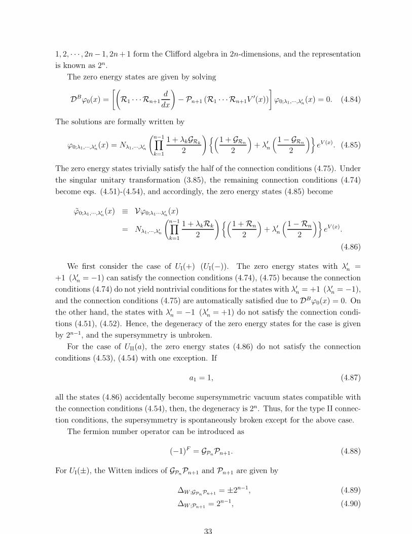
The zero energy states are given by solving

DBϕ0(x) =

[(

R1 · · ·Rn+1d

dx

)

−Pn+1 (R1 · · ·Rn+1V′(x))

]

ϕ0;λ1,···,λ′n(x) = 0. (4.84)

The solutions are formally written by

ϕ0;λ1,···,λ′n(x) = Nλ1,···,λ′n

(n−1∏

k=1

1 + λkGRk

2

){(1 + GRn

2

)

+ λ′n

(1− GRn

2

)}

eV (x). (4.85)

The zero energy states trivially satisfy the half of the connection conditions (4.75). Under

the singular unitary transformation (3.85), the remaining connection conditions (4.74)

become eqs. (4.51)-(4.54), and accordingly, the zero energy states (4.85) become

ϕ0;λ1,···,λ′n(x) ≡ Vϕ0;λ1···λ′n(x)

= Nλ1,···,λ′n

(n−1∏

k=1

1 + λkRk

2

){(1 +Rn

2

)

+ λ′n

(1−Rn

2

)}

eV (x).

(4.86)

We first consider the case of UI(+) (UI(−)). The zero energy states with λ′n =

+1 (λ′n = −1) can satisfy the connection conditions (4.74), (4.75) because the connection

conditions (4.74) do not yield nontrivial conditions for the states with λ′n = +1 (λ′n = −1),

and the connection conditions (4.75) are automatically satisfied due to DBϕ0(x) = 0. On

the other hand, the states with λ′n = −1 (λ′n = +1) do not satisfy the connection condi-

tions (4.51), (4.52). Hence, the degeneracy of the zero energy states for the case is given

by 2n−1, and the supersymmetry is unbroken.

For the case of UII(a), the zero energy states (4.86) do not satisfy the connection

conditions (4.53), (4.54) with one exception. If

a1 = 1, (4.87)


the connection conditions (4.54), then, the degeneracy is 2n. Thus, for the type II connec-

tion conditions, the supersymmetry is spontaneously broken except for the above case.

The fermion number operator can be introduced as

(−1)F = GPnPn+1. (4.88)

For UI(±), the Witten indices of GPnPn+1 and Pn+1 are given by

∆W ;GPnPn+1 = ±2n−1, (4.89)

∆W ;Pn+1 = 2n−1, (4.90)

33

where the double sign in eq. (4.89) correspond to the double sign in the UI(±). For UII(a),

the Witten index of GPnPn+1 vanishes because the zero energy states do not exist. Let us

comment on the special case (4.87), where we have the zero energy states. We note that

the supersymmetry is enhanced to the same N = 2n + 1 supersymmetry in the special

case as that in the previous section.

5 Summary

In this paper, we have studied the supersymmetry on a circle with 2n point singularities

placed at regular intervals in a full detail. The two types of the N = 2n+1 supercharges

(type A and type B) are constructed in terms of the n+1 sets of discrete transformations

{Pk,Qk,Rk} (k = 1, 2, · · · , n + 1). The singularities can be described by the connection

conditions in our formulation. We have found the connection conditions make all the

supercharges physical, so that the N = 2n+ 1 supersymmetry can be realized under the

connection conditions.

In our analysis, the connection conditions, under which arbitrary subset of the N =

2n + 1 supercharges are physical and others are not physical, can be obtained. Thus,

the N = 2n + 1 supersymmetry can be reduced to M-extended supersymmetry for any

integer M < N due to the connection conditions.

We have also studied the degeneracy of the spectrum in particular zero energy states

in the N = 2n + 1 supersymmetric models and some N = 2n supersymmetric models as

examples of the reduction of the supersymmetry. The energy eigenfunctions can be labeled

by the eigenvalues of the physical operators which commute with the Hamiltonian and

each other. The degeneracy of the spectrum for the states with E > 0 have been obtained

by discussing the transition of the labeled states under the action of the supercharges.

The analysis cannot apply for the states with E = 0. This is because the zero energy

states satisfy Qϕ0 = 0, that is, the transition does not occurs. The zero energy states,

however, satisfy the first order differential equation thanks to the supersymmetry, and the

formal solutions can be obtained. We have checked whether the formal solutions satisfy

the connection conditions or not. The degeneracy of the spectrum and the Witten index

are summarized in table 1 and table 2.

Acknowledgements

The authors wish to thank C.S. Lim, I. Tsutsui for valuable discussions and useful

comments. M. S. is supported in part by the Grant-in-Aid for Scientific Research

(No.15540277) by the Japanese Ministry of Education, Science, Sports and Culture. K.

T. is supported in part by the Grant-in-Aid for Science Research, Ministry of Education,

Science and Culture, Japan, No. 17043007 and the 21st Century COE Program at Osaka

University.

34

Table 1: degeneracy of the spectrum in the N = 2n+ 1 supersymmetric modelsType parameters degeneracy Witten index

Type Ab2 = 0and

E > 12c2 2n+1

W ′′(x) = 0(W ′(x) ≡ c)

E = 12c2

{

2n for b1 = +10 for b1 = −1

∆W ;Pn+1 = 2n

(for b1 = 1)

otherwise E > 0 2n

E = 0

{

2n for ∗0 for otherwise

0

Type B b2 = 0 E > 0 2n+1

E = 0

{

2n for b1 = +10 for b1 = −1

∆W ;Pn+1 = 2n

(for b1 = 1)otherwise E > 0 2n

E = 0 0 0

where ∗ denotes√

1−b21+b2

= e2W (l0−ǫ).

References

[1] M. Reed, B. Simon, “Methods of Modern Mathematical Physics”, Vol.II, AcademicPress, New York, 1980.

[2] P. Seba, Czeck. J. Phys. 36 (1986) 667.

[3] S. Albeverio, F. Gesztesy, R. Høegh-Krohn, H. Holden, “Solvable Models in QuantumMechanics”, Springer, New York, 1988.

[4] T. Cheon, T. Shigehara, Phys. Rev. Lett. 82 (1999) 2536, quant-ph/9806041.

[5] I. Tsutsui, T. Fulop, T. Cheon, J. Phys. Soc. Jap. 69 (2000) 3473, quant-ph/0003069.

[6] T. Cheon, Phys. Lett. A248 (1998) 285, quant-ph/9803020.

[7] P. Exner, H. Grosse, “Some properties of the one-dimensional generalized point in-teractions (a torso), math-ph/9910029.

[8] T. Cheon, T. Fulop, I. Tsutsui, Ann. Phys. 294 (2001) 1, quant-ph/0008123.

[9] T. Uchino, I. Tsutsui, Nucl. Phys. B662 (2003) 447, quant-ph/0210084.

[10] T. Nagasawa, M. Sakamoto, K.Takenaga, Phys. Lett. B562 (2003) 358, hep-th/0212192.

[11] T. Uchino, I. Tsutsui, J. Phys. A36 (2003) 6493, hep-th/0302089.

[12] T. Nagasawa, M. Sakamoto, K. Takenaga, Phys. Lett. B583 (2004), 357, hep-th/0311043.

[13] M. Shaposhnikov and P. Tinyakov, Phys. Lett. B515 (2001), 442, hep-th/0102161.

35

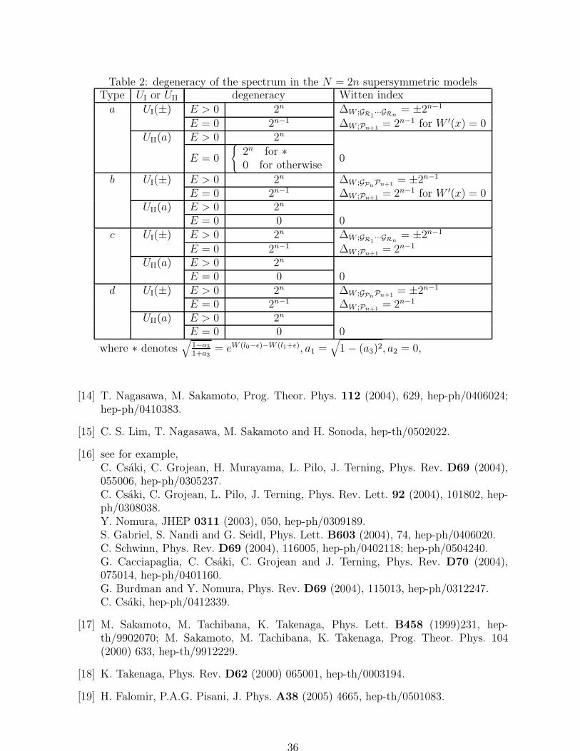
Table 2: degeneracy of the spectrum in the N = 2n supersymmetric modelsType UI or UII degeneracy Witten indexa UI(±) E > 0 2n ∆W ;GR1

···GRn= ±2n−1

E = 0 2n−1 ∆W ;Pn+1 = 2n−1 for W ′(x) = 0UII(a) E > 0 2n

E = 0

{

2n for ∗0 for otherwise

0

b UI(±) E > 0 2n ∆W ;GPnPn+1 = ±2n−1

E = 0 2n−1 ∆W ;Pn+1 = 2n−1 for W ′(x) = 0UII(a) E > 0 2n

E = 0 0 0c UI(±) E > 0 2n ∆W ;GR1

···GRn= ±2n−1

E = 0 2n−1 ∆W ;Pn+1 = 2n−1

UII(a) E > 0 2n

E = 0 0 0d UI(±) E > 0 2n ∆W ;GPnPn+1 = ±2n−1

E = 0 2n−1 ∆W ;Pn+1 = 2n−1

UII(a) E > 0 2n

E = 0 0 0

where ∗ denotes√

1−a31+a3

= eW (l0−ǫ)−W (l1+ǫ), a1 =√

1− (a3)2, a2 = 0,

[14] T. Nagasawa, M. Sakamoto, Prog. Theor. Phys. 112 (2004), 629, hep-ph/0406024;hep-ph/0410383.

[15] C. S. Lim, T. Nagasawa, M. Sakamoto and H. Sonoda, hep-th/0502022.

[16] see for example,C. Csaki, C. Grojean, H. Murayama, L. Pilo, J. Terning, Phys. Rev. D69 (2004),055006, hep-ph/0305237.C. Csaki, C. Grojean, L. Pilo, J. Terning, Phys. Rev. Lett. 92 (2004), 101802, hep-ph/0308038.Y. Nomura, JHEP 0311 (2003), 050, hep-ph/0309189.S. Gabriel, S. Nandi and G. Seidl, Phys. Lett. B603 (2004), 74, hep-ph/0406020.C. Schwinn, Phys. Rev. D69 (2004), 116005, hep-ph/0402118; hep-ph/0504240.G. Cacciapaglia, C. Csaki, C. Grojean and J. Terning, Phys. Rev. D70 (2004),075014, hep-ph/0401160.G. Burdman and Y. Nomura, Phys. Rev. D69 (2004), 115013, hep-ph/0312247.C. Csaki, hep-ph/0412339.

[17] M. Sakamoto, M. Tachibana, K. Takenaga, Phys. Lett. B458 (1999)231, hep-th/9902070; M. Sakamoto, M. Tachibana, K. Takenaga, Prog. Theor. Phys. 104(2000) 633, hep-th/9912229.

[18] K. Takenaga, Phys. Rev. D62 (2000) 065001, hep-th/0003194.

[19] H. Falomir, P.A.G. Pisani, J. Phys. A38 (2005) 4665, hep-th/0501083.

36

Documents

on a circle with point singularities - arXiv · on a circle with point singularities ... [email protected] ... the upper ﬁgures mean the geometrical meaning of Pk,Rk