Material and Methods

3.1 Material

3.1.1. Plant materials

The plant material used in the present study comprised of a total of 15 important

accessions of genus Ocimum placed within five species. The seed material for all the

accessions was obtained from National gene bank of CIMAP, as described in (Table 3.1).

Table: 3.1. Description of planting materials employed in the present study

Accession Source of seeds Ocimum species Germplasm OCS1 CIMAP, Lucknow Ocimum tenuiflorum CIM-Ayu/HYDOCS2 CIMAP, RC, Hyderabad O. tenuiflorum CIM-Kanchan/HydOCS3 CIMAP, RC, Hyderabad O. tenuiflorum OTP-Tall/HydOCS4 CIMAP, Lucknow O. tenuiflorum CIM-Angana/LkoOCS5 CIMAP, Lucknow O. tenuiflorum CIM-Amrit/LkoOCS6 CIMAP, Lucknow O. tenuiflorum Nasik/LkoOCB7 CIMAP, RC, Hyderabad O. basilicum LO/HydOCB8 CIMAP,RC, Hyderabad O. basilicum LM-IV/HydOCB9 CIMAP,RC, Hyderabad O. basilicum OB5/OBT/HydOCB10 CIMAP, RC, Hyderabad O. basilicum OB4/EXO/HydOCB11 CIMAP,RC, Hyderabad O. basilicum Soumya/HydOCA12 CIMAP,RC, Hyderabad O. americanam CTRL-II/HydOCG13 CIMAP,RC, Hyderabad O. gratissimum OGO/HydOCG14 CIMAP,RC, Hyderabad O. gratissimum OGM/HydOCK15 CIMAP,RC, Hyderabad O. kilimandscharicum OK/Hyd

Among the various genotypes, six accessions were from O. tenuiflorum L.f. (syn.

O. sanctum L.), five accessions were of O. basilicum L., two accessions were from O.

gratissimum L. and a single accession each was from O. kilimandscharicum Baker ex.

Guerke and Ocimum canam Sim. syn. O. amricanam were selected for the study. Initially,

most of these accessions were maintained at CIMAP Resource Centre, Hyderabad (AP),

except few accessions that were maintained at CIMAP Lucknow (UP). The G x E

interaction and phenotypic stability analysis was performed for important characters of

Ocimum accessions grown in the field conditions across two consecutive years (2007 to

2009) and three locations (Lucknow, Hyderabad and Bangalore) as shown in the (Figure

3.1). The average data from the observations were used for morphological characterization,

statistical derivation and interpretation in the study.

Page | 34

Material and Methods

Page | 35

Figure: 3.1. Three different Agro-environment (Lucknow,Hyderabad and Bangalore) of study for Ocimum species germplasm accessions.

Agro-ecological locations of India

Material and Methods

3.1.2. Chemicals and reagents

Chemicals and reagents used in the present study were procured from various

manufacturing companies viz., Sigma Aldrich (USA), High media (India), Difco (USA),

Merk (Germany), BioLabs (India), Thermo Scientific (India) etc.

CTAB, Tris-HCl, NaCl, chloroform, phenol, isopropanol, TAE, ethanol, high salt

TE, sterilized-H2O, PVP (Sigma), EDTA, dNTPs (Fermentas), Taq polymerase, PCR buffer

(Fermentas), RAPD Primer (Operon technologies, USA), ISSR primers (Ocimum

Biosolution, Hyderabad), 100 bp DNA molecular marker (BioLabs), Agarose (High Media),

Loading dye and Ethidium bromide, SDS, Dimethylsulfoxide, Anhydrous sodium sulphate,

HPLC grade H2O, culture media for bacterial and fungal growth and standard antibiotic discs

were purchased from Hi-Media. McFarland Standard solution, Nutrient agar and broth,

Mueller-Hinton agar, Sabaroud’s dextrose agar etc. were used in the study.

Buffers, solutions and media

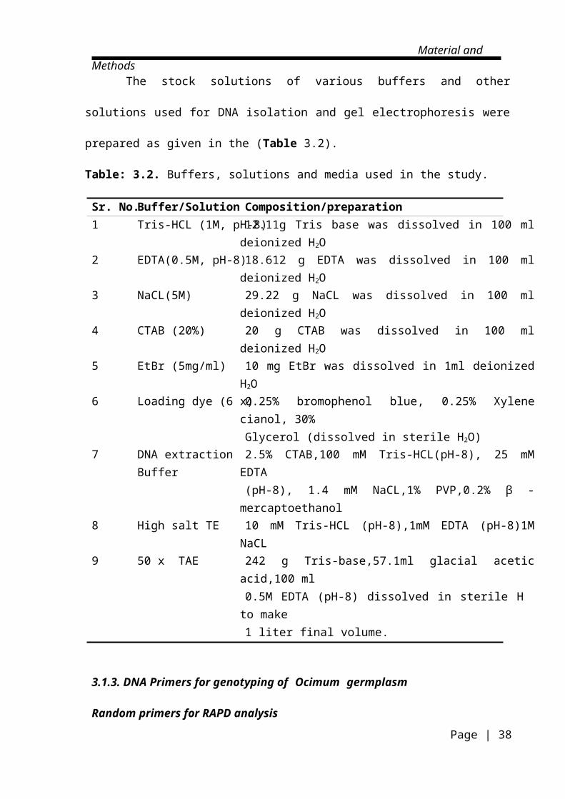
The stock solutions of various buffers and other solutions used for DNA isolation

and gel electrophoresis were prepared as given in the (Table 3.2).

Table: 3.2. Buffers, solutions and media used in the study.

Sr. No. Buffer/Solution Composition/preparation1 Tris-HCL (1M, pH-8) 12.11g Tris base was dissolved in 100 ml deionized H2O2 EDTA(0.5M, pH-8) 18.612 g EDTA was dissolved in 100 ml deionized H2O3 NaCL(5M) 29.22 g NaCL was dissolved in 100 ml deionized H2O4 CTAB (20%) 20 g CTAB was dissolved in 100 ml deionized H2O5 EtBr (5mg/ml) 10 mg EtBr was dissolved in 1ml deionized H2O6 Loading dye (6 x) 0.25% bromophenol blue, 0.25% Xylene cianol, 30%

Glycerol (dissolved in sterile H2O)7 DNA extraction

Buffer2.5% CTAB,100 mM Tris-HCL(pH-8), 25 mM EDTA (pH-8), 1.4 mM NaCL,1% PVP,0.2% β -mercaptoethanol

8 High salt TE 10 mM Tris-HCL (pH-8),1mM EDTA (pH-8)1M NaCL9 50 x TAE 242 g Tris-base,57.1ml glacial acetic acid,100 ml

0.5M EDTA (pH-8) dissolved in sterile H2O to make 1 liter final volume.

Page | 36

Material and Methods

3.1.3. DNA Primers for genotyping of Ocimum germplasm

Random primers for RAPD analysis

Seventeen random decamer primers which were used for the characterization and

RAPD profiling of germplasm in this study are described in the (Table 3.3)

Table: 3.3. List of RAPD primers used for germplasm characterization and phylogenetic analysis.

Sr. No Primer Sequence 5’-----3’1 OPO-6 CCA CGG GAA G2 OPO-9 TCC CAC GCA A3 0PO-11 GAC AGG AGG T4 OPO-13 GTC AGA GTC C5 OPO-14 AGC ATG GCT C6 OPO-15 TGG CGT CCT T7 OPO-16 TCG GCG GTT C8 OPO-17 GGC TTA TGC C9 OPO-18 CTC GCT ATC C10 OPO-19 GGT GCA CGT T11 OPO-20 ACA CAC GCT G12 OPT-2 GGA GAG ACT C13 OPT-12 GGG TGT GTA G14 OPT-13 AGG ACT GCC A15 OPT-16 GGT GAA CGC T16 OPT-17 CCA ACG TCG T17 OPT-18 GAT GCC AGA C

ISSR Primers

ISSR markers have unique efficiency in distinguishing even closely related

germplasm accessions. In this study, eight ISSR primers which were used for genotyping

of Ocimum germplasm are described in (Table 3.4).

Table: 3.4. List of ISSR primers for phylogenetic analysis

Sr. No Primer Sequence5’-----3’

Primer length Tm

1 Micro-8 (CAA)5 15 40.62 Micro-13 (GTGA)4 16 40.03 Micro-16 (GAAT)4 16 40.04 Micro-19 (GACA)4 16 44.85 G-13 (GTG)5 15 48.06 G-18 (ACG)5 15 57.07 M-6 (GTC)5 15 61.48 C-12 (GAC)5 15 56.0

Page | 37

Material and Methods

3.1.4. Bacterial strains

Eight bacteria comprising gram positive and gram negative strains which were used

for determination of antibacterial activity of the essential oils from various Ocimum species

and their accessions are described in (Table 3.5).

Table: 3.5. Bacterial strains used in the antibacterial bioassay of Ocimum essential oils.

Sr. No Bacterial strain Type of bacteriaName MTCC No.

1 Staphylococcus aureus MTCC96 Gram positiveGram positiveGram positiveGram positive

2 Streptococcus mutans MTCC4973 Bacillus subtilis MTCC1214 Salmonella typhi MTCC7335 Klebsiella pneumonia MTCC109 Gram negative

Gram negativeGram negativeGram negative

6 Escherichia coli MTCC7237 Micrococcus luteus MTCC24708 Raoultella planticola MTCCRP530

The above bacterial cultures were procured from the Microbial Type Culture

Collection Centre (MTCC), CSIR-Institute of Microbial Technology (CSIR-IMTech),

Chandigarh and are currently maintained in the Bio Safety Division of CSIR-CIMAP,

Lucknow, India.

3.1.5. Instruments

The instruments used for different analysis during the study are as follows. Laminar

air flow (Newton), Ultra low Freezer-80 (NBS), Electronic Balance (Sartorius, India),

Water bath (RMS Lauda), Labtherm shaker (Kuhner), Autoclave (Tomy, USA), High

speed refrigerated centrifuge (Sigma), PCR Machine (Bio-Rad), UV Trans-illuminator

(Fotodyne), Gel documentation system (Pharmacia Biotech), Spectrophotometer

(Beckman), Nanodrop (ND1000), Clevenger apparatus (Borosil glass), Gas

Chromatography-Perkin-Elmer (8700), Mortar and Pestle, cooler freezer (Geni), deep

freezer -20 (vest frost), submarine electrophoresis units (Bio Labs), pH meter (Lab India),

Digital Camera (Nicon).

Page | 38

Material and Methods

3.1.6. Glasswares and plasticwares

All the glasswares used in the present study viz., spreading glass rod,

culture tubes, oil collection tubes, conical flask, beakers, measuring cylinder, schott duran

bottles etc. were purchased from Borosil, India. The plasticwares such as digital micro

pipettes (Nichipet ECO, USA) and micro tips (Genaxy, India), Micro-centrifuge tubes

(Eppendorf, USA), Powder free latex gloves and 90 mm plastic petri plates (Genaxy, India)

were used in the study.

3.1.7. Statistical software and databases

CIMAP Ver. 1.0 for D2 and other statistical analysis, SPSS ver. 17, free tree

software, treeview 32, and Sigma plot ver. 14, Microsoft office word 2007 and Microsoft

office excel 2007 were used for the statistical analysis of the experimental data.

3.2. Methods

3.2.1. Experimental location and edapho-climatic conditions

In order to evaluate the G x E interaction, genetic diversity among different Ocimum

germplasm and stability of genotypes, field experiments were conducted at three locations of

the India, namely (1). CIMAP Research Centre, Hyderabad [altitude 542 m above mean sea

level -(MSL), latitude 17o25’ N, and longitude 78o33’ E); mean annual rainfall as 764 mm

(80% of which is received between June and September); winter season characterized by

mild, cool, dry weather. (2). CIMAP Lucknow (Semiarid-to Subtropical climate, located at

128 m above MSL, latitude 26’8’N and longitude 80.9 E); mean annual rainfall as 800 mm

(80-85% of which is received between July to September) and (3). CIMAP Research Centre,

Bangalore (altitude 930 m above mean sea above MSL, latitude 13o05’ N and longitude

77o55’ E). The area receives a mean annual rainfall of 870 mm, between May and October.

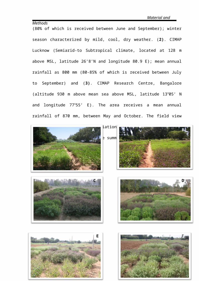
The field view (Figure 3.2) and climatic variation of all the three locations during the

experimentation are summarized in (Table 3.6)

Page | 39

Material and Methods

3.2.2. Experimental field design

Figure: 3.2. Experimental field view of Ocimum crop at full blooming stage at Hyderabad (A and

B), Lucknow (C and D) and Bangalore (E and F) locations.

Page | 40

BA

C D

E F

Material and Methods

The experiment was laid out in Randomized Block Design (RBD) on well-drained

soil at all the locations by using the method as prescribed by Sidney, A. (1970). All the

fifteen Ocimum germplasm accessions were transplanted in the respective locations with

three replications for two consecutive cropping years (2007-2008 and 2008-2009).

Individual plot size was 2.5 × 3 m (7.5 m2). Each plot received vermin-compost (1-2 t/ha),

single superphosphate (P2O5 40 kg.ha-1), and muriate of potash (K2O 40 kg.ha-1) prior to

planting. Seeds of all the fifteen Ocimum germpalsm were sown in nursery beds in June

first week at all the three experimental locations. Six weeks old, uniformly growing,

healthy seedlings were transplanted at 60 cm row-to-row and 45 cm plant-to-plant spacing

(Rao et al., 2011) during third week of July at all the experimental locations. The fields

were irrigated after planting and thereafter, at 10 to 12 day intervals. Nitrogen (as urea) was

given at 50 kg/ha for each harvest. Weeds were manually removed 25 and 45 days after

transplanting seedlings, and after each harvest.

Metric observations

The morphometric data for the following growth and yield contributing traits were

recorded on 10 randomly selected plants from all the blocks for characterization and

evaluation of G x E interaction and phenotypic stability in Ocimum germplasm accessions

over the years. All the traits were measured at full flowering stage of crop emphasizing the

morphological characters viz., plant height (cm), plant canopy (cm), No. of primary

branches, leaf length (cm), leaf width (cm), leaf area (cm2), leaf stem ratio (fresh wt basis),

essential oil content (% w/ v), fresh herb yield (t/ha) and essential oil yield (lit/ha).

Page | 41

Material and Methods

Harvesting of crop

Crop was harvested manually 10-15 cm above the ground level (Singh, et al., 2013)

during each growing season at all the respective locations having full bloom stage (Gupta

et al.,1996).

3.2.3. Morphological characterization of Ocimum germplasm

The important qualitative morphological characters for characterization of germplasm

accessions were observed before harvesting of crops. Quantitative morphological data viz.,

plant height, plant canopy, number of primary branches, fresh biomass/plant, leaf length,

leaf width, leaf area, essential oil content, 1000 seeds weight, spike length and number of

whorls/spike recorded for Hyderabad experimental location were subjected for

phenotyping and used to calculate Euclidean distance (Ed) for all pairs of accessions.

Euclidean distance obtained from 11 morphological traits was used to construct

hierarchical dendogram with the help of SPSS statistical software ver.17. Principal

Component Analysis (PCA) was performed to demonstrate the relationship among Ocimum

germplasm accessions in terms of their position relative to two coordinate axes. PCA using

correlated data matrix among phenotypic traits was used to determine differences between

accessions.

3.2.4. Chemotypic characterization and diversity analysis

For the extraction of essential oil, after every harvest aerial shoots biomass (leaf,

branches and inflorescence) weighing approximately 300 g was collected from every block

at each location and hydro distilled using Clevenger’s apparatus (Clevenger, 1928) for 3 h.

Essential oil concentration (%) was estimated using formula-

EOC = Essential oil (ml) recovered/ weight of biomass (g) ×100.

Essential oil yield per unit area was calculated by multiplying the biomass yield

with essential oil concentration (Clevenger’s data) and density of the essential oil. Essential

Page | 42

Material and Methods

oil samples were dried over anhydrous sodium sulphate and stored in sealed glass vials at

40C till further analysis.

Gas chromatography

Gas chromatography (GC) usually represents the method of choice nowadays to

scrutinize the complex mixture of an essential oil (Cserháti, 2010). Volatile oil samples were

analyzed on a PerkinElmer (PerkinElmer Life and Analytical Sciences, Milano, Italy) Gas

Chromatography (auto system XLGC) machine having flame ionization detector (FID), an

electronic integrator, and bonded phased fused silica capillary column (60 meters x 0.32 mm

id x 0.25 mm film thickness); Capillary column coated with polydimethylsiloxane was

employed as the stationary phase. Hydrogen was the carrier gas with 0.4 ml/min flow rate

and 10 psi column pressure. The oven temperature was programmed initially at 700C (2min)

and increased at 250oC at 3oC/min (hold time 2 min) and 290oC at 6oC /min ramp rate and 10

min hold time. Injector and detector were set at 280oC and 350oC, respectively. Samples

(0.06 mL) were injected neat with split ratio 1:80.

Identification of essential oil constituents

Essential oil components were identified by comparing their retention times with

authentic compounds run under identical conditions, by comparison of retention indices

(Kováts, 1965) computed from gas chromatograms by logarithmic interpolation between n-

alkanes. Homologous series of n-alkanes C8-C22, Poly Science Inc. Niles, USA, were used

as standard) with literature data and comparison of peaks’ mass spectra with standard

compounds reported in literature and stored on NIST and Wiley MS libraries. Quantitative

data was obtained by electronic integration of peak areas without the use of response

correction factors:

Page | 43

Material and Methods

3.2.5. Chemotypic diversity analysis through Euclidean distance model

Quantitative data of the major essential oil components obtained from GC analysis

were used to calculate the Euclidean distance (Ed) for all pairs of samples.

Where i and j represent two cases (samples) of the data matrix, k represents the variable

(chemical compound) and the total number of variables is n. Cluster analysis was used to

classify and group all the germplasm according to their main components. Cluster analysis

based on selected components and was calculated using the Euclidean distance measure.

For the grouping of the chemotypes, the agglomerative and hierarchical method was

applied (Ozdemir, 2002) using the single linkage method. Principal Component Analysis

(PCA) was performed to display the relationship among Ocimum germplasm accessions in

terms of their position relative to two dimensional coordinate system. PCA using correlated

data matrix among essential oil constituents was used to determine differences between

accessions.The computations were performed using SPSS package software (Version 17).

3.2.6. DNA fingerprinting for molecular genetic diversity analysis

The diversity due to genetic constitution of germplasm accessions was analyzed by

employing PCR amplification profile of DNA with random primers and microsatellite

primers ISSR.

Isolation of genomic DNA

Total genomic DNA was isolated from the young apical leaves of all 15 Ocimum

germplasm accessions grown at Lucknow location, using CTAB method described by

Porebsky et al. (1997). Well cleaned and fine tissue powder of leaves grounded in liquid

nitrogen was extracted using CTAB buffer (2.5% CTAB, 100 mM Tris-Hcl (pH 8), 25 mM

EDTA (pH8), 1.5M NaCl, 1% PVP, 0.3% b-mercapto-ethanol) and incubated at 650C for

one hour. Chloroform: iso-amylalcohol (24:1) was added to the incubated sample and

Page | 44

Material and Methods

mixed by inversion up to 15 min. to form an emulsion, centrifuged at 10,000 rpm for 10

minutes at room temperature. The upper layer (supernatant) was transferred and

precipitated by adding 5 M NaCl (1/25th vol.) and 0.6 volume of isopropanol. DNA was

pelleted at 10,000 rpm for 10 min, washed with 80% ethanol, dried and resuspended in

high salt TE buffer (10 mM, Tris-HCl (pH-8.0) and 1M-NaCl). This DNA was again

extracted with chloroform/ isoamyl alcohol (24:1), and then the supernatant was transferred

and precipitated with ice-cold absolute alcohol. This was followed by a centrifugation at

12,000 rpm for 10 min at 40C and washing with 70% ethanol. The dried pellets were

dissolved in 50µl sterile distilled water. The quality and concentration of DNA were

estimated using a DNA ladder of known concentration and absorbance at 260 nm and

working stocks of DNA were prepared based on both the estimates.

PCR and amplification of Genomic DNA

DNA fingerprinting by RAPD

Decamer arbitrary oligonucleotides (Operon technologies, USA) were used for PCR

amplification following the procedure of Williams et al. (1990) and Khanuja et al. (1998)

with a few modifications. Amplification were performed in 25 µl volume of PCR reaction

mixture containing 25-50 ng genomic DNA as template, 0.6 unit of Taq polymerase, 100

µM of each of the dNTPs, 2.0 µl 10 x buffer, 1 µl of MgCl2 (15mM) and 5 pmol of primers.

The PCR were performed in a thermo- cycler programmed as follows.

Step 1: Initial denaturation at 940C for 5min

Step 2: Denaturation at 940C for 1.0 min

Annealing at 38.40C for 1.0 min

Extension at 720C for 2.0 min

Step 3: Final extension at 720C for 5 min

Page | 45

45 cycles

Material and Methods

DNA fingerprinting by ISSR

Inter simple sequence repeat (ISSR) are the primers anchored at the 5' or 3' end of a

repeat region and extend into the flanking region. This technique allows amplification of

the genomic segments between inversely oriented repeats (ISSRs). Generally, a series of

single primers are used to generate series of fragments that are size-separated on either an

agarose gel or polyacrylamide. The same volume and concentration of reaction mixture

(mentioned for RAPD) was employed for ISSR amplifications. The PCR programming for

amplification is as follows:

Step 1: Initial denaturation at 940C for 5 min

Step 2: Denaturation at 940C for 1min

Annealing at 420C* for 2 min

Extension at 720C for 1 min

Step 3: Final extension at 720C for 5 min.

The annealing temperatures were optimized for each primer used. A rough estimate of the

annealing temperature (Tm) for the primer was calculated by using the following formula

(Suggs et al., 1981)

Tm = (G + C) ×4°C + (A + T) ×2°C

Where G, C, A and T are the numbers of these nucleotides in the primer, respectively.

(*Annealing temperature was set according to Tm value of used primers).

Gel electrophoresis

The amplification products (RAPD and ISSR) were differentiated by horizontal gel

electrophoresis using 1.4 % agarose in 0.5X TAE buffer and 20 μl amplicon product of

each sample with 2μl loading dye (1 times concentrated) was loaded on the agarose gel.

DNA marker of 100 bp was used to estimate molecular weight and size of the fragments.

Gel Electrophoresis was run for 3 hours at 100 V. The DNA was stained with (0.5mg/ml)

Page | 46

40 cycles

Material and Methods

ethidum bromide (EtBr) which was mixed with warmed agarose gel before pouring in

casting tray. The gels were photographed with Image master VDS (Pharmacia).

3.2.7. Statistical analysis of RAPD and ISSR profile for genetic diversity

RAPD and ISSR profiles/bands were scored manually for each individual accession

from the gel photograph. The bands were recorded as discrete characters, presence ‘1’ or

absence ‘0’ and ‘?’for missing and ambiguous data. The resulting presence/absence data

matrix of the RAPD and ISSR were analyzed by using FreeTree software to estimate

genetic diversity parameters such as; the percentage of polymorphic bands (PPB) and the

genetic standard distance (Ds) between populations were computed using the formula

given by (Nei's, 1972).

To examine the genetic relationship among populations, a dendrogram was also

constructed by an un-weighted paired group method of cluster analysis using arithmetic

averages (UPGMA). Jaccard’s coefficient was calculated by using FREETREE software,

common estimator of genetic identity and similarities were calculated as follows:

Jaccard’s coefficient = NAB / (NAB+ NA+ NB)

Where NAB is the number of bands shared by samples, NA represents fragments in

sample B. Similarity matrices based on these indices were calculated. Similarity matrices

were utilized to construct the UPGMA (un-weighted pair group method to construct

arithmetic average) dendogram. Statistical stability of the branches in the cluster was

estimated by bootstrap analysis with 1,000 replicates, using the Tree-Free software

program.

3.2.8. Antibacterial bioassay

Disk-diffusion assay (Bauer et al., 1996) was conducted to get an idea about the

antibacterial activity of essential oil of Ocimum germplasm collections against some

selected pathogenic microbes. The inoculums of the test microbes were prepared up to a

Page | 47

Material and Methods

density equivalent to the McFarland Standard 0.5. Uniform lawn of each of the test bacteria

(Gram positive and Gram negative bacteria) were prepared using 100 ml inoculum of the

specified bacteria on nutrient agar plate. The filter paper (What man No.6 were soaked with

neat essential oil (8 µl) and placed over the seeded plates. The plates were incubated at

37oC for 24 hrs. The activity was measured in terms of zone of microbial growth inhibition.

The net zone of inhibition was determined by subtracting the disc diameter (6.0 mm) from

the total zone of inhibition shown by the test disc in terms of clear zone around the disc.

3.2.9. Statistical analysis of agro-morphological traits for genetic divergence study

The statistical analysis of 10 economic traits was performed with the help of

analysis of variance (ANOVA) technique (statistical software CIMAP ver.1. based on

(Singh and Chaudhary, 1979) as applicable to Randomized Block Design (Panse and

Sukhatme, 1978). Variance (F) ratio was applied to test the significance of treatment

variance versus error variance. Least significant difference (LSD) values at 5% and 1%

probability level (5% and 1%) were computed by multiplying standard error of difference

(SED) values with tabulated t values, for assessing the significance of differences between

any two treatment means.

Analysis of variance (ANOVA)

Xijk =m+gi + rj + eijk

Where, Xijk is kth observation in jth replication of ith treatment (genotypes) , m is the grand

mean gi is the effect of ith genotype (treatment), rj is the effect of block jth replication. eijk is

the environmental effect associated with ijk th observation.

Source Main effect Degree of freedom Mean squre F (expected)

Block (Replications) r-1 Rms Rms /Ems

Treatment (Genotypes) g-1 Gms Ems (Gms-Ems)/r

Error (r-1)(g-1)

Page | 48

Material and Methods

Correlation coefficient:

Correlation coefficient between independent (x) and dependent (y) variables were

calculated at phenotypic (rp), genotypic (rg) and environmental (re) levels using variance

and covariance from sub-section A as under.

rp = Cov (p) xy/ . ) 1/2, rg = Cov (g) xy/ . ) 1/2, re = Cov (e) xy/ . ) ½

Multivariate analysis

The genetic divergence among 15 Ocimum accessions was determined on the basis

of ten characteristics using Mahalanobis (1936) D2 statistic and canonical analysis (Rao,

1952) as follows;

D2 statistic

The Mahalanobi’s generalized distance (D2) between any two populations is defined

as:

D2= ∑ ∑ λij di dj

Where,ij-The matrix reciprocal to the common dispersion matrix (error variance and

covariance) and di and dj were the difference between the mean values of the two

populations for ith and jth characters, respectively. The analyses were involved as following

steps:

Assessment of component of variance among the accessions

Variance due to genotypes, i.e. the genotypic variance

was calculated as the difference (MSG-MSE) over number of replications, i.e. =

(MSG-MSE)

Page | 49

Material and Methods

Phenotypic variance ):

Phenotypic variance being the sum total of the variation among genotypes and the

environmental variation was calculated as = +

Heritability in broad sense ( 2 (bs)

It was calculated as the ratio of total genotypic variance to the phenotypic variance in

broad sense ( 2 (bs)) as 2

(bs) = + (Lush, 1948).

Genetic advance (GA)

It was calculated by following formula (Robinson, 1949).

GA = i x 2 (bs) x

Where, i is the standardized selection differential (i.e. the difference in mean of a

genotype from the base population means at 1% selection intensity, i.e. I =2.64),) 2 (bs) and

are the usual notations described above.

Computation of D2 values

The D2 values representing divergence between two accessions were obtained as the

sum of squares of differences in the value of y’s associated with the two genotypes for each

component.

Group constellation:

(i) The grouping by visual observation of the relative size of D2 between any two accessions,

and (ii) Final grouping confirmed by Tocher’s (Rao, 1952)

Intra and inter cluster divergence:

Page | 50

Material and Methods

After final grouping, the intra-cluster divergence was obtained from the last column

of Tocher’s table itself. The inter-cluster divergence was calculated by averaging the total

D2 values between any two accessions included in different clusters. The cluster means for

each character were calculated by averaging each of the x’s values for all genotypes

included in each cluster.

Canonical analysis

The spatial distances among individual accession could also be determined by

canonical analysis. For this the uncorrelated y-variables obtained under D2 statics were

further exploited. λ1- λ2 chart were prepared by the first two canonical vectors supplied

the best two linear functions Z1 and Z2. Since λ1+ λ2 accounted for more than 70 % of the

total variance, λ1- λ2 was found to be adequate. Further, the y-values and then mean value

of Z1 and Z2 were calculated. The two dimensional representation was depicted having the

canonical variation λ1 and λ2 as the coordinate axes.

3.2.10. G x E interaction and stability analysis

In order to analyses the Gene x Environment interaction, the comparative

expression patterns of distinct characters were studied across the locations. The stability

model proposed by Eberhart and Russell (1966) was adopted to analyze the data over three

environments. The model involves the estimation of three stability parameters like mean

(µi), regression coefficient (bi) and deviation from regression (S2di), which are defined by

the following mathematical formula.

Yij = µi + βiIj + ij

Yij: Mean of ith genotype at the jth environment (i=1, 2, 3, 4, 5….22, j = 1, 2, 3)

μi: The mean of ith genotype over all the environments

Page | 51

Material and Methods

∑i: The regression coefficient that measures the response of i th genotype to varying

environment

∑ij: The deviation from regression of the ith genotype of jth environment

Ij: The environmental index obtained by subtracting the regression of the ith

Stability parameters

The mean (µi), the regression coefficient (bi) and mean square deviation from linear

regression line (S2di) are the three stability parameters proposed by Eberhart and Russell

(1966) in their stability model. These parameters were computed by using the following

formula.

a) Genotype the grand mean from the mean of all genotype at jth environment.

µi (mean) = ∑jYij / s

b) Environmental index Ij

Ij =

Where, t = Number of varieties, s = Number of environments with jIj = 0

c) The regression coefficient for each germplasm.

bi =

(d) Deviation from regression S2di =

Where, S2e/r = Mean square for (estimate of) pooled error

(e) Predicted performance of the genotypes

Yij = + biIj

Page | 52

Material and Methods

Where, is the estimate of bi

In this model the variance due to environments and Genotype × Environment (G x E) are

partitioned into environment (linear), genotype × environment (linear) and deviations from

the regression coefficient.)

ANOVA for stability

Source of variation D.F SS MS F valueGenotypes (G) (g-1) SiSjY2ij -CF MS1 MS1/MS3Environment (E) (n-1) 1/nSjY2i – 1/n SjY2iG x E (g-1)(n-1) SiSj Y2ij – 1/nSjY2iEnvironment (linear) 1 1/g [(SjYj - Ij)2 SjIj2 ]Genotype x Environment (Linear)

(g-1) Sj [(S Yij Ij)2 / Sj Ij2]- 1/g [(SjYj - Ij)2 SjIj2]

MS2 MS2/MS3

Pooled deviation g (n-2) Si Sj d2ij2 MS3 MS3/MS4Pooled error n(g-1)(r-1) MS4Total (ng – 1) Si Sj Y Ij2 – CF TSSWhere,

n = Number of environments, r = Number of replications

g = Number of genotypes, CF = Correction factor

(a) To test the significance of pooled deviation mean square against the pooled error mean

square

F = MS3/ MS4

If pooled deviation mean square is found significant then it is the appropriate denominator

to test the significance of all components including genotypes, genotype G x E

environment (linear). Otherwise pooled error mean square is appropriate denominator.

(b) To test the significance of the differences among the means of genotypes.

F = MS1/ MS3

(c) To test that the genotypes do not differ for their regression on environmental index

F = MS2/ MS3

Further, t’ test was used to test the significance of deviation of ‘bi’ from unity

t =1-bi / S.E (bi)

Page | 53

Material and Methods

Where ,

SE (bi) =

ij is the deviation of ith variety in jth environment from regression

d) To test individual deviation from linear regression

F = / Pooled error mean square

A joint consideration of three parameters, that is;

(i) The mean performance of the genotype over environments (location),

(ii) Regression coefficient bi and

(iii) The deviation from linear regression S2di, are used to define stability of genotype

(variety).

The estimate of deviation from regression suggests the degree of reliance that should be put

to linear regression in interpretation of data. If these values are significantly deviating from

zero, the expected phenotype cannot be predicted satisfactorily. When deviations are non

significant, the conclusions, may be drawn by joint consideration of mean yield and

regression values (Finlay and Wilkinson (1963) and Eberhart and Russell (1966) as

described below;

Regression Stability Mean yield

Remarks

bi = 1 Average High Well adapted to all the environments

bi = 1 Average Low Poorly adapted to all environments

bi > 1 Below average High Specifically adopted to favourableenvironments

Page | 54

Material and Methods

bi < 1 Above average High Specifically adopted to unfavourableenvironments

Page | 55