Olink Wizard for GenEx USER GUIDE

Version 1.0 (June 2013)

TECHNICAL SUPPORT For support and technical information, please contact support@multid.se, or join the GenEx online forum: www.multid.se/forum.php.

Table of content

1. INTRODUCTION………………………………………………… ……… 4

2. EXPORTING DATA FROM THE FLUIDIGM BIOMARK……………………….. 5

3. OLINK WIZARD FOR GENEX……………………………………………… 9

4. NORMALIZATION METHOD……………………………………………… 18

5. LINEAR VALUES………………………………………………… ……… 19

3

The Olink wizard add-on feature for GenEx is an easy-to-use data import and pre-processing tool. The wizard will guide you through all steps of importing data, validating data quality and normalization of your Proseek Multiplex data, preparing it for statistical analysis with the GenEx software. In short: ►Export your data from the Fluidigm BioMark ►Follow the Olink wizard for GenEx for quality control and normalization of your data Continue with statistical analysis of your data, such as hierarchical clustering methods, principal component analysis and more using the GenEx software.

1. Introduction

4

2. Exporting data from the Fluidigm Biomark

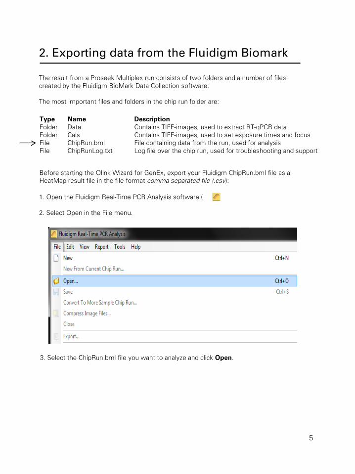
The result from a Proseek Multiplex run consists of two folders and a number of files created by the Fluidigm BioMark Data Collection software: The most important files and folders in the chip run folder are: Type Name Description Folder Data Contains TIFF-images, used to extract RT-qPCR data Folder Cals Contains TIFF-images, used to set exposure times and focus File ChipRun.bml File containing data from the run, used for analysis File ChipRunLog.txt Log file over the chip run, used for troubleshooting and support

Before starting the Olink Wizard for GenEx, export your Fluidigm ChipRun.bml file as a HeatMap result file in the file format comma separated file (.csv):

1. Open the Fluidigm Real-Time PCR Analysis software ( ). 2. Select Open in the File menu.

3. Select the ChipRun.bml file you want to analyze and click Open.

5

4. Add sample information using Sample Setup according to manufacturer’s instruction (www.fluidigm.com). Sample names can also be provided later in GenEx. 5. Biomarker names are inserted automatically in the Olink wizard for GenEx. 6. Optional: For a quick overview of the data, use the built in functions of the Fluidigm Real-Time PCR Analysis software according to manufacturer’s instruction (www.fluidigm.com). 7. IMPORTANT! Make sure that the baseline correction in the Fluidigm RT-PCR Analysis Software is set to Linear and that the Ct Threshold Method is set to Auto (Global) under “Analysis views”. In versions up to 3.X this is the standard setting. When changing this setting you need to click the Analyze button before exporting the data. Auto (Global) Threshold is used to avoid differences in dCq values between biomarkers depending on where the threshold is set for each run. It is possible to use other methods for setting the threshold as well, but this might prove to flag samples as outliers in the wizard. If you decide to change this setting, keep it in mind when comparing several runs and also when going through the quality control of the wizard.

6

9. Name your data file in the File name box. 10. Select Heat Map Results (*.csv) in the Save as type menu.

8. Select Export in the File menu to export your data.

7

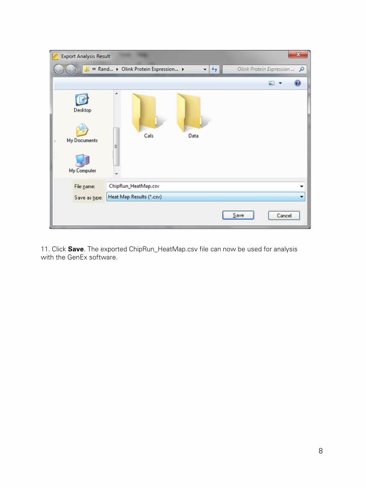
11. Click Save. The exported ChipRun_HeatMap.csv file can now be used for analysis with the GenEx software.

8

3. Olink Wizard for Genex 1. Start the GenEx software. 2. Press the Olink Wizard icon.

3. The Olink Wizard start screen is displayed. Click Next.

9

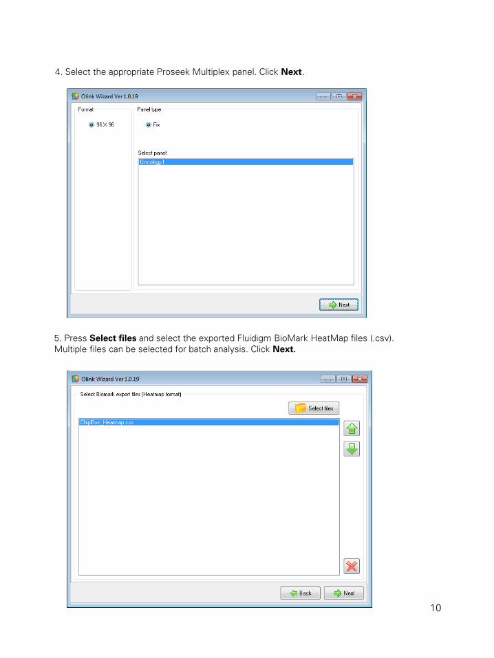
4. Select the appropriate Proseek Multiplex panel. Click Next.

5. Press Select files and select the exported Fluidigm BioMark HeatMap files (.csv). Multiple files can be selected for batch analysis. Click Next.

10

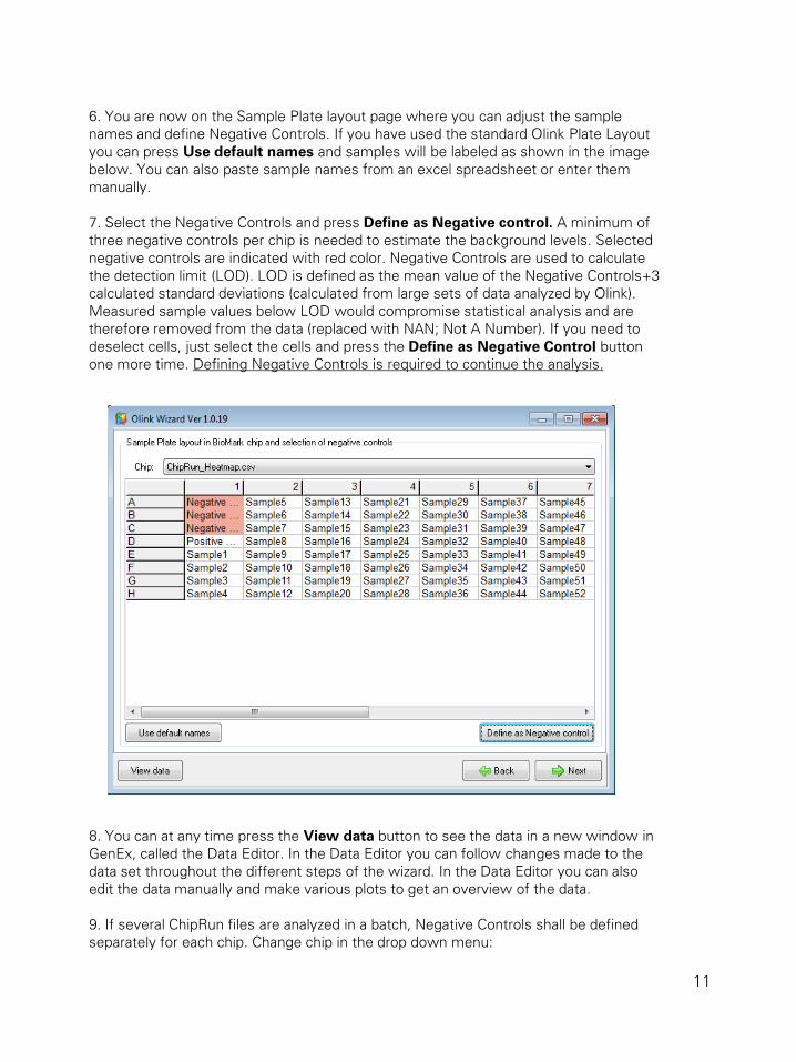
8. You can at any time press the View data button to see the data in a new window in GenEx, called the Data Editor. In the Data Editor you can follow changes made to the data set throughout the different steps of the wizard. In the Data Editor you can also edit the data manually and make various plots to get an overview of the data. 9. If several ChipRun files are analyzed in a batch, Negative Controls shall be defined separately for each chip. Change chip in the drop down menu:

6. You are now on the Sample Plate layout page where you can adjust the sample names and define Negative Controls. If you have used the standard Olink Plate Layout you can press Use default names and samples will be labeled as shown in the image below. You can also paste sample names from an excel spreadsheet or enter them manually. 7. Select the Negative Controls and press Define as Negative control. A minimum of three negative controls per chip is needed to estimate the background levels. Selected negative controls are indicated with red color. Negative Controls are used to calculate the detection limit (LOD). LOD is defined as the mean value of the Negative Controls+3 calculated standard deviations (calculated from large sets of data analyzed by Olink). Measured sample values below LOD would compromise statistical analysis and are therefore removed from the data (replaced with NAN; Not A Number). If you need to deselect cells, just select the cells and press the Define as Negative Control button one more time. Defining Negative Controls is required to continue the analysis.

11

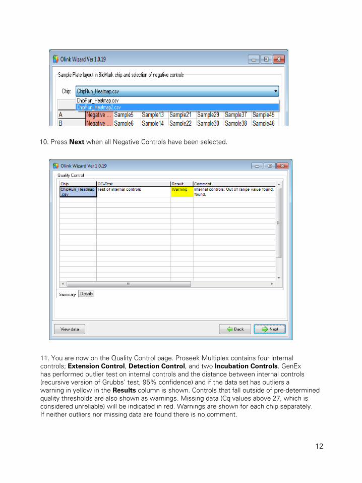
11. You are now on the Quality Control page. Proseek Multiplex contains four internal controls; Extension Control, Detection Control, and two Incubation Controls. GenEx has performed outlier test on internal controls and the distance between internal controls (recursive version of Grubbs’ test, 95% confidence) and if the data set has outliers a warning in yellow in the Results column is shown. Controls that fall outside of pre-determined quality thresholds are also shown as warnings. Missing data (Cq values above 27, which is considered unreliable) will be indicated in red. Warnings are shown for each chip separately. If neither outliers nor missing data are found there is no comment.

10. Press Next when all Negative Controls have been selected.

12

12. Select the Details tab in the lower left corner to see detailed information for each chip. Here individual outliers are shown and can be removed from the analysis. Look through highlighted values and decide if the sample need to be removed from analysis. The measured values for each internal control should not vary across samples:

13

13. Select samples to be removed (if any) from analysis by checking the corresponding boxes in the Remove column, and press Remove selected samples from analysis. 14. Press Next when done.

a. Ext Ctrl: The Extension Control monitors the PEA (Proximity Extension Assay) reaction. This control is used for normalization and compensates for PEA, PCR and qPCR variations between samples. b. Det Ctrl: The Detection Control monitors the PCR and qPCR step. This control is not affected during incubation or extension and is therefore used for detection of outliers and technical errors. c. dCq Incubation: dCq Incubation shows the difference between one of the Incubation Controls and the Detection Control. The two Incubation Controls are two control immunoassays measuring spiked antigens. They measure the variation in the incubation step of the assay. d. dCq Extension: dCq Extension is the difference between the Detection Control and the Extension Control.

15. You are now on the Overview of Data page. Here you can view your data in three different control charts. Select chart type by the radio buttons on the Chart type tab. Switch to the Page options tab to change settings or to scroll pages. The available control charts are: a. Box plot: Each box and whisker shows the distribution of the measured sample values of one protein across the samples. The red dotted line indicates the median value.

14

b. Limit of Detection and missing data frequency: A bar chart shows the fraction of samples with values below the Limit of Detection and frequency of missing data for each biomarker.

15

c. Sample value profiles: Profile plots shows variation of the measured sample values for selected biomarkers.

16. Inspect the QC charts and identify any odd behaving sample or biomarker. You can click View data at any time to inspect the individual data in the GenEx editor and decide to remove samples or biomarkers from the analysis. In the editor you can also index suspicious samples and later test how they influence the results of analysis. Press Next to proceed. 17. You are now on the final page of the wizard where you can replace missing data and sample value data below LOD, with corresponding LOD value. This serves two purposes. Firstly, no significance is attributed to difference in measurement bellow LOD; all those values are treated equal. Secondly, many multivariate statistical methods require full sets of data and cannot be used on data sets with missing values. If you select No Action you can handle missing data later in the GenEx editor or limit analysis to univariate methods that handle missing data.

16

18. Press Next.

The data import, normalization and quality control in the Olink wizard is now completed. Your data set will next be displayed in the GenEx Data Editor. There you can perform additional pre-processing steps before statistical analysis, see the GenEx User Guide.

17

4. Normalization method Cq values from the Fluidigm run are imported into the wizard. The pre-processing steps convert the imported Cq values (log2 scale where lower values correspond to higher protein levels) to ddCq values (still in log2 scale but now lower values correspond to lower protein levels). a) The first step performed is normalization against the Extension Control. The dCq value will still be on log2 scale where a low value corresponds to low protein concentration. dCqanalyte = Cqanalyte – CqExtension Control b) The second step calculates the difference between the dCq values and a negative control determined at Olink. The generated ddCq will now be on log2 scale where a high value corresponds to high protein concentration. ddCq = dCqOlink negative - dCqanalyte

18

5. Linear values Cq values are logarithmic and a difference of one Cq value between two samples correspond to approx twice the amount of protein detected. Small differences in Cq can be quite large in linear values. For manual analysis, or just to get an overview of the data, it can be easier to look at linear values. Convert your ddCq values to linear values by using this formula: 2 ddCq. For calculating Coefficient of Variation (%CV) between replicate samples, you need to use linear values.

19

Olink Bioscience Dag Hammarskjölds v. 52B

SE-752 37 Uppsala, Sweden www.olink.com

The following trademarks are owned by Olink AB: Olink®, Olink BioscienceTM, and Proseek®. The following trademarks are owned by MultiD: MultiDTM and GenExTM. Copyright © 2013 Olink AB.

0964

, v.1

.0,

2013

-06-

11