Oligopolies and Nash

Equilibrium

Anna Nagurney

Isenberg School of Management

University of Massachusetts

Amherst, MA 01003

c©2002

Oligopoly theory dates to Cournot (1838), who investi-gated competition between two producers, the so-calledduopoly problem, and is credited with being the first tostudy noncooperative behavior.

In an oligopoly, it is assumed that there are several firms,which produce a product and the price of the productdepends on the quantity produced.

Examples of oligopolies include large firms in computer,

automobile, chemical or mineral extraction industries,

among others.

1

Nash (1950, 1951) subsequently generalized Cournot’s

concept of an equilibrium for a behavioral model con-

sisting of n agents or players, each acting in his/her

own self-interest, which has come to be called a nonco-

operative game. Specifically, consider m players, each

player i having at his/her disposal a strategy vector

xi = {xi1, . . . , xin} selected from a closed, convex set

Ki ⊂ Rn, with a utility function ui : K 7→ R1, where K =

K1×K2×. . .×Km ⊂ Rmn. The rationality postulate is that

each player i selects a strategy vector xi ∈ Ki that max-

imizes his/her utility level ui(x1, . . . , xi−1, xi, xi+1, . . . , xm)

given the decisions (xj)j 6=i of the other players.

2

In this framework one then has:

Definition 1 (Nash Equilibrium)

A Nash equilibrium is a strategy vector

x∗ = (x∗1, . . . , x

∗m) ∈ K,

such that

ui(x∗i , x̂

∗i ) ≥ ui(xi, x̂

∗i ), ∀xi ∈ Ki,∀i, (1)

where x̂∗i = (x∗

1, . . . , x∗i−1, x∗

i+1, . . . , x∗m).

3

It has been shown (cf. Hartman and Stampacchia (1966)and Gabay and Moulin (1980)) that Nash equilibria sat-isfy variational inequalities. In the present context, un-der the assumption that each ui is continuously differ-entiable on K and concave with respect to xi, one has

Theorem 1 (Variational Inequality Formulation ofNash Equilibrium)

Under the previous assumptions, x∗ is a Nash equilibriumif and only if x∗ ∈ K is a solution of the variationalinequality

〈F (x∗), x − x∗〉 ≥ 0, ∀x ∈ K, (2)

where F (x) ≡ (−∇x1u1(x), . . . ,−∇xmum(x)) is a row vec-

tor and where ∇xiui(x) = (∂ui(x)∂xi1

, . . . , ∂ui(x)∂xin

).

Proof: Since ui is a continuously differentiable functionand concave with respect to xi, the equilibrium condi-tion (1), for a fixed i, is equivalent to the variationalinequality problem

−〈∇xiui(x∗), xi − x∗

i 〉 ≥ 0, ∀xi ∈ Ki, (3)

which, by summing over all players i, yields (2).

4

If the feasible set K is compact, then existence is guar-

anteed under the assumption that each ui is contin-

uously differentiable. Rosen (1965) proved existence

under similar conditions. Karamardian (1969), on the

other hand, relaxed the assumption of compactness of

K and provided a proof of existence and uniqueness of

Nash equilibria under the strong monotonicity condition.

As shown by Gabay and Moulin (1980), the imposition

of a coercivity condition on F (x) will guarantee exis-

tence of a Nash equilibrium x∗ even if the feasible set is

no longer compact. Moreover, if F (x) satisfies the strict

monotonicity condition, uniqueness of x∗ is guaranteed,

provided that the equilibrium exists.

5

Classical Oligopoly Problems

We now consider the classical oligopoly problem in whichthere are m producers involved in the production of ahomogeneous commodity. The quantity produced byfirm i is denoted by qi, with the production quantitiesgrouped into a column vector q ∈ Rm. Let fi denotethe cost of producing the commodity by firm i, and letp denote the demand price associated with the good.Assume that

fi = fi(qi) (4)

and

p = p(m∑

i=1

qi). (5)

The profit for firm i, ui, can then be expressed as

ui(q) = p(m∑

i=1

qi)qi − fi(qi). (6)

6

Assuming that the competitive mechanism is one ofnoncooperative behavior, in view of Theorem 1, onecan write down immediately:

Theorem 2 (Variational Inequality Formulation ofClassical Cournot-Nash Oligopolistic Market Equi-librium)

Assume that the profit function ui(q) is concave withrespect to qi, and that ui(q) is continuously differen-tiable. Then q∗ ∈ Rm

+ is a Nash equilibrium if and only ifit satisfies the variational inequality

m∑i=1

[∂fi(q∗i )

∂qi− ∂p(

∑mi=1 q∗i )

∂qiq∗i − p(

m∑i=1

q∗i )

]× [qi − q∗i ] ≥ 0,

∀q ∈ Rm+. (7)

7

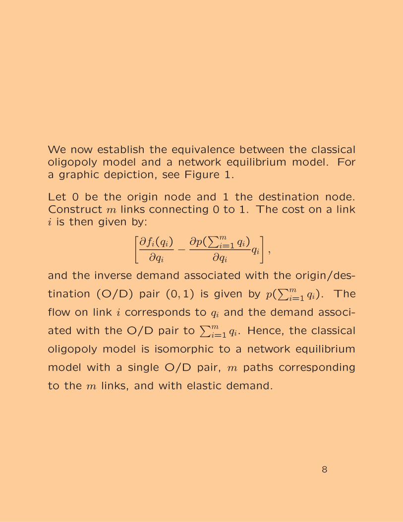
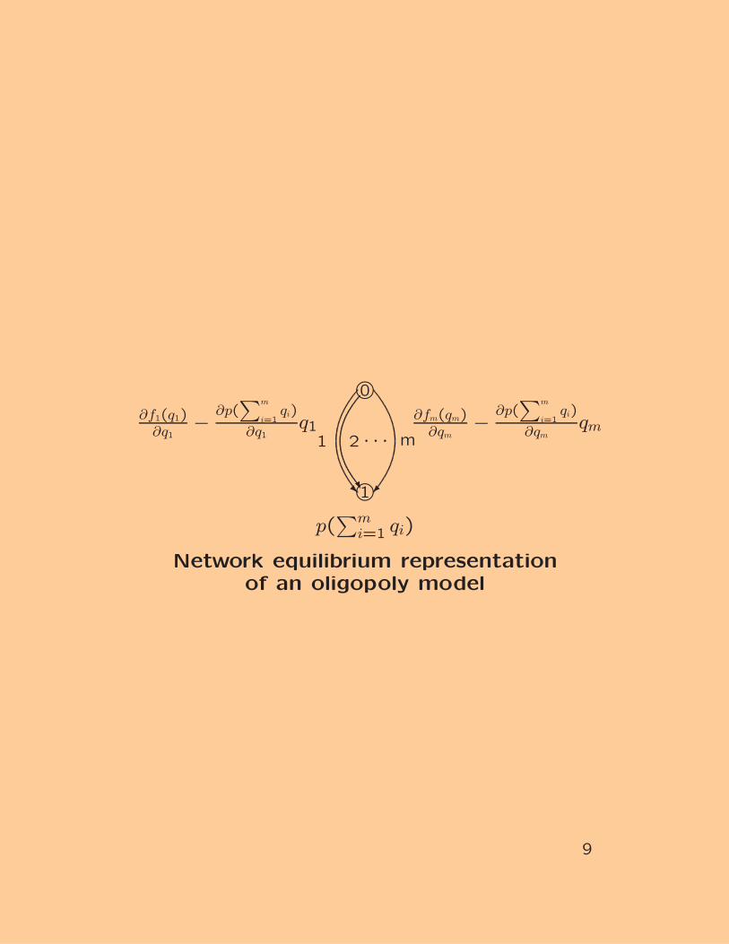
We now establish the equivalence between the classicaloligopoly model and a network equilibrium model. Fora graphic depiction, see Figure 1.

Let 0 be the origin node and 1 the destination node.Construct m links connecting 0 to 1. The cost on a linki is then given by:[

∂fi(qi)

∂qi− ∂p(

∑mi=1 qi)

∂qiqi

],

and the inverse demand associated with the origin/des-

tination (O/D) pair (0,1) is given by p(∑m

i=1 qi). The

flow on link i corresponds to qi and the demand associ-

ated with the O/D pair to∑m

i=1 qi. Hence, the classical

oligopoly model is isomorphic to a network equilibrium

model with a single O/D pair, m paths corresponding

to the m links, and with elastic demand.

8

m

m

1

0

R U

1 2 · · · m

∂f1(q1)∂q1

− ∂p(∑m

i=1qi)

∂q1q1

∂fm(qm)∂qm

− ∂p(∑m

i=1qi)

∂qmqm

p(∑m

i=1 qi)

Network equilibrium representationof an oligopoly model

9

Computation of Classical Oligopoly Problems

First consider a special case of the oligopoly model

described above, characterized by quadratic cost func-

tions, and a linear inverse demand function. The for-

mer model has received attention in the literature (cf.

Gabay and Moulin (1980), and the references therein),

principally because of its stability properties. It is now

demonstrated that a demand market equilibration al-

gorithm can be applied for the explicit computation of

the Cournot-Nash equilibrium pattern. The algorithm is

called the oligopoly equilibration algorithm, OEA. After

its statement, it is applied to compute the solution to a

three-firm example.

10

Assume a quadratic production cost function for eachfirm, that is,

fi(qi) = aiq2i + biqi + ei, (8)

and a linear inverse demand function, that is,

p(m∑

i=1

qi) = −o

m∑i=1

qi + r, (9)

where ai, bi, ei, o, r > 0, for all i. Then the expression forthe cost on link i is given by: (2ai + o)qi + bi, for alli = 1, . . . , m.

The oligopoly equilibration algorithm is now stated.

OEA

Step 0: Sort

Sort the bi’s; i = 1, . . . , m, in nondescending order andrelabel them accordingly. Assume, henceforth, that theyare relabeled. Also, define bm+1 ≡ ∞ and set I := 1. Ifb1 ≥ r, stop; set qi = 0; i = 1, . . . , m, and exit; otherwise,go to Step 1.

Step 1: Computation

Compute

λI =

ro+

∑Ii=1

bi

(2ai+o)

1o+

∑Ii=1

1(2ai+o)

. (10)

11

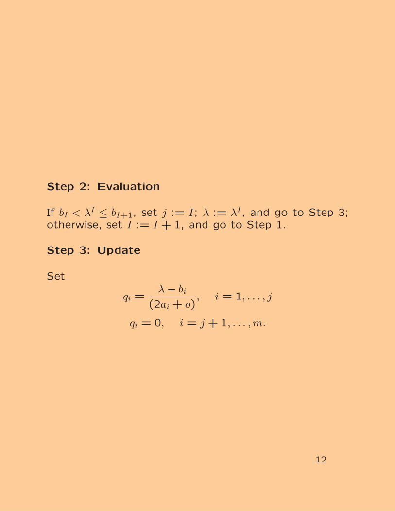
Step 2: Evaluation

If bI < λI ≤ bI+1, set j := I; λ := λI, and go to Step 3;otherwise, set I := I + 1, and go to Step 1.

Step 3: Update

Set

qi =λ − bi

(2ai + o), i = 1, . . . , j

qi = 0, i = j + 1, . . . , m.

12

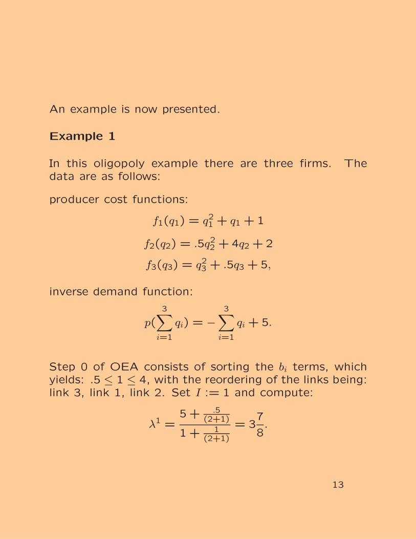
An example is now presented.

Example 1

In this oligopoly example there are three firms. Thedata are as follows:

producer cost functions:

f1(q1) = q21 + q1 + 1

f2(q2) = .5q22 + 4q2 + 2

f3(q3) = q23 + .5q3 + 5,

inverse demand function:

p(3∑

i=1

qi) = −3∑

i=1

qi + 5.

Step 0 of OEA consists of sorting the bi terms, whichyields: .5 ≤ 1 ≤ 4, with the reordering of the links being:link 3, link 1, link 2. Set I := 1 and compute:

λ1 =5 + .5

(2+1)

1 + 1(2+1)

= 37

8.

13

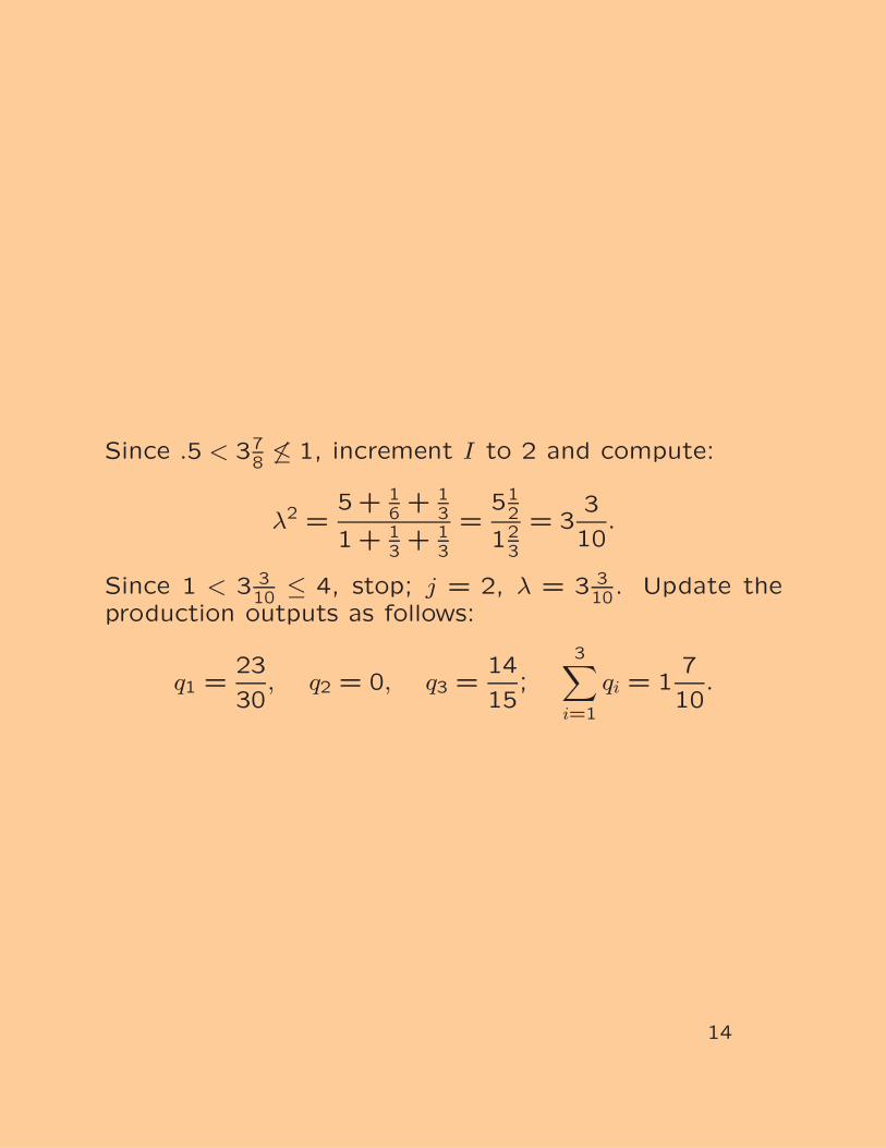
Since .5 < 3786≤ 1, increment I to 2 and compute:

λ2 =5 + 1

6+ 1

3

1 + 13+ 1

3

=51

2

123

= 33

10.

Since 1 < 3 310

≤ 4, stop; j = 2, λ = 3 310

. Update theproduction outputs as follows:

q1 =23

30, q2 = 0, q3 =

14

15;

3∑i=1

qi = 17

10.

14

We now turn to the computation of Cournot-Nash equi-libria in the case where the production cost functions (4)are not limited to being quadratic, and the inverse de-mand function (cf. (5)) is not limited to being linear.In particular, an oligopoly iterative scheme is presentedfor the solution of variational inequality (7) governingthe Cournot-Nash model. It is then shown that thescheme induces the projection method and the relax-ation method; each of these methods, in turn, decom-poses the problem into very simple subproblems.

The Iterative Scheme

Construct a smooth function g(q, y) : Rm+ × Rm

+ 7→ Rm

with the following properties:

(i). g(q, q) = −∇Tu(q), ∀q ∈ Rm+.

(ii). For every q ∈ Rm+, y ∈ Rm

+, the m×m matrix ∇qg(q, y)is positive definite.

15

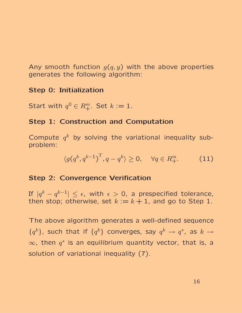
Any smooth function g(q, y) with the above propertiesgenerates the following algorithm:

Step 0: Initialization

Start with q0 ∈ Rm+. Set k := 1.

Step 1: Construction and Computation

Compute qk by solving the variational inequality sub-problem:

〈g(qk, qk−1)T, q − qk〉 ≥ 0, ∀q ∈ Rm

+. (11)

Step 2: Convergence Verification

If |qk − qk−1| ≤ ε, with ε > 0, a prespecified tolerance,then stop; otherwise, set k := k + 1, and go to Step 1.

The above algorithm generates a well-defined sequence

{qk}, such that if {qk} converges, say qk → q∗, as k →∞, then q∗ is an equilibrium quantity vector, that is, a

solution of variational inequality (7).

16

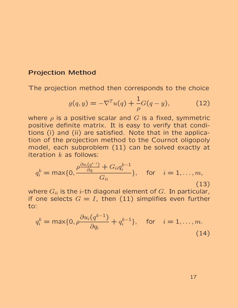
Projection Method

The projection method then corresponds to the choice

g(q, y) = −∇Tu(q) +1

ρG(q − y), (12)

where ρ is a positive scalar and G is a fixed, symmetricpositive definite matrix. It is easy to verify that condi-tions (i) and (ii) are satisfied. Note that in the applica-tion of the projection method to the Cournot oligopolymodel, each subproblem (11) can be solved exactly atiteration k as follows:

qki = max{0,

ρ∂ui(qk−1)∂qi

+ Giiqk−1i

Gii}, for i = 1, . . . , m,

(13)where Gii is the i-th diagonal element of G. In particular,if one selects G = I, then (11) simplifies even furtherto:

qki = max{0, ρ

∂ui(qk−1)

∂qi+ qk−1

i }, for i = 1, . . . , m.

(14)

17

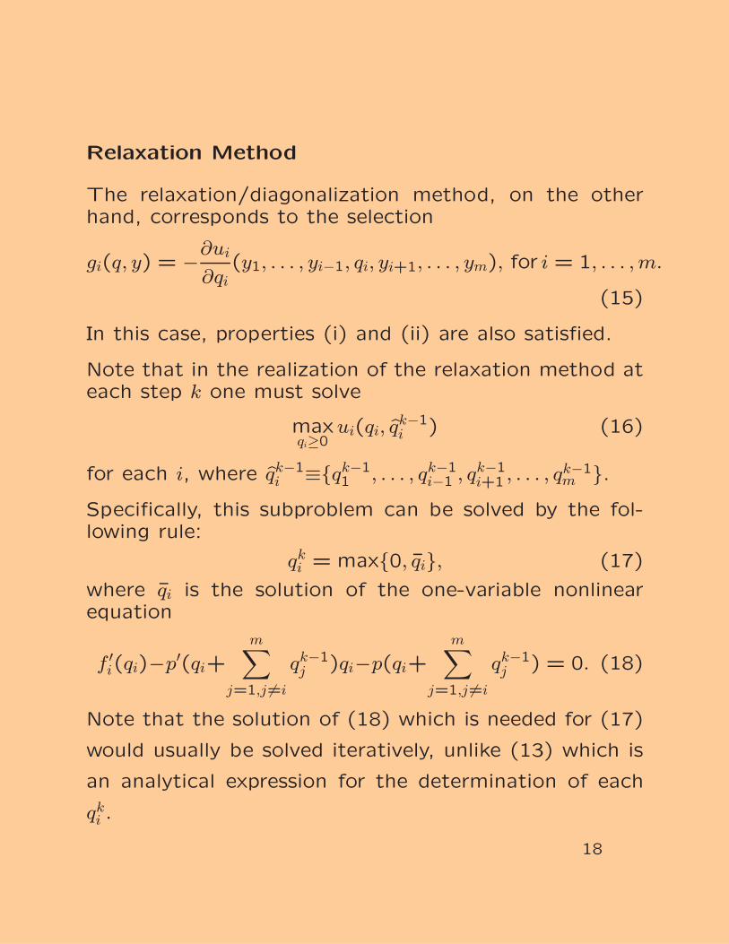
Relaxation Method

The relaxation/diagonalization method, on the otherhand, corresponds to the selection

gi(q, y) = −∂ui

∂qi(y1, . . . , yi−1, qi, yi+1, . . . , ym), for i = 1, . . . , m.

(15)

In this case, properties (i) and (ii) are also satisfied.

Note that in the realization of the relaxation method ateach step k one must solve

maxqi≥0

ui(qi, q̂k−1i ) (16)

for each i, where q̂k−1i ≡{qk−1

1 , . . . , qk−1i−1 , qk−1

i+1 , . . . , qk−1m }.

Specifically, this subproblem can be solved by the fol-lowing rule:

qki = max{0, q̄i}, (17)

where q̄i is the solution of the one-variable nonlinearequation

f ′i(qi)−p′(qi+

m∑j=1,j 6=i

qk−1j )qi−p(qi+

m∑j=1,j 6=i

qk−1j ) = 0. (18)

Note that the solution of (18) which is needed for (17)

would usually be solved iteratively, unlike (13) which is

an analytical expression for the determination of each

qki .

18

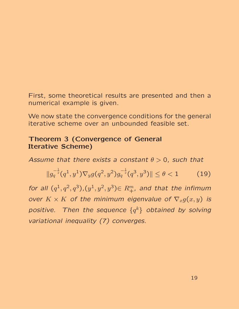
First, some theoretical results are presented and then anumerical example is given.

We now state the convergence conditions for the generaliterative scheme over an unbounded feasible set.

Theorem 3 (Convergence of GeneralIterative Scheme)

Assume that there exists a constant θ > 0, such that

‖g−1

2q (q1, y1)∇yg(q

2, y2)g−1

2q (q3, y3)‖ ≤ θ < 1 (19)

for all (q1, q2, q3),(y1, y2, y3)∈ Rm+, and that the infimum

over K × K of the minimum eigenvalue of ∇xg(x, y) is

positive. Then the sequence {qk} obtained by solving

variational inequality (7) converges.

19

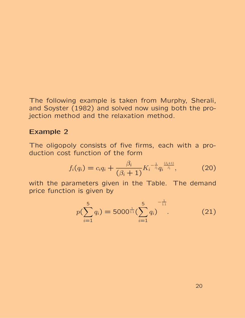
The following example is taken from Murphy, Sherali,and Soyster (1982) and solved now using both the pro-jection method and the relaxation method.

Example 2

The oligopoly consists of five firms, each with a pro-duction cost function of the form

fi(qi) = ciqi +βi

(βi + 1)Ki

− 1

βi qi

(βi+1)

βi , (20)

with the parameters given in the Table. The demandprice function is given by

p(5∑

i=1

qi) = 50001

1.1(5∑

i=1

qi)

− 1

1.1

. (21)

20

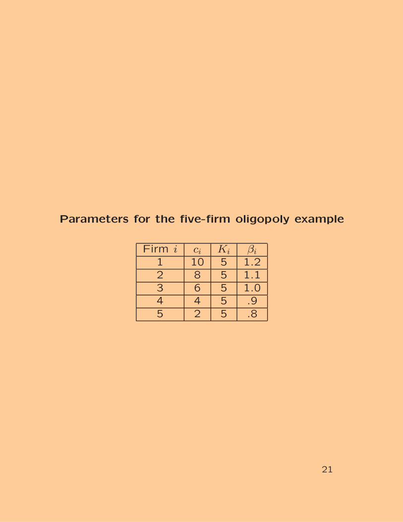
Parameters for the five-firm oligopoly example

Firm i ci Ki βi

1 10 5 1.22 8 5 1.13 6 5 1.04 4 5 .95 2 5 .8

21

Both the projection method and the relaxation methodwere implemented in FORTRAN, compiled using theFORTVS compiler, optimization level 3. The conver-gence criterion was |qk

i − qk−1i | ≤ .001, for all i, for both

methods. A bisecting search method was used to solvethe single variable problem (17) for each firm i, in therelaxation method. The matrix G was set to the iden-titiy matrix I for the projection method with ρ = .9.The system used was an IBM 3090/600J at the Cor-nell Theory Center. Both algorithms were initialized atq0 = (10,10,10,10,10).

The projection method required 33 iterations but only

.0013 CPU seconds for convergence, whereas the re-

laxation method required only 23 iterations, but .0142

CPU seconds for convergence. Both methods converged

to q∗=(36.93,41.81,43.70,42.65,39.17), reported to the

same number of decimal places.

22

A Spatial Oligopoly Model

Now a generalized version of the classical oligopoly modelis presented. Assume that there are m firms and n de-mand markets that are generally spatially separated. As-sume that the homogeneous commodity is produced bythe m firms and is consumed at the n markets. As be-fore, let qi denote the nonnegative commodity outputproduced by firm i and now let dj denote the demandfor the commodity at demand market j. Let Tij de-note the nonnegative commodity shipment from supplymarket i to demand market j. Group the productionoutputs into a column vector q ∈ Rm

+, the demands intoa column vector d ∈ Rn

+, and the commodity shipmentsinto a column vector T ∈ Rmn

+ .

The following conservation of flow equations must hold:

qi =n∑

j=1

Tij, ∀i (22)

dj =m∑

i=1

Tij, ∀j (23)

where Tij ≥ 0, ∀i, j.

23

As previously, associate with each firm i a productioncost fi, but allow now for the more general situationwhere the production cost of a firm i may depend uponthe entire production pattern, that is,

fi = fi(q). (24)

Similarly, allow the demand price for the commodity ata demand market to depend, in general, upon the entireconsumption pattern, that is,

pj = pj(d). (25)

Let tij denote the transaction cost, which includes thetransportation cost, associated with trading (shipping)the commodity between firm i and demand market j.Here we permit the transaction cost to depend, in gen-eral, upon the entire shipment pattern, that is,

tij = tij(T). (26)

The profit ui of firm i is then

ui =n∑

j=1

pjTij − fi −n∑

j=1

tijTij. (27)

In view of (22) and (23), one may write

u = u(T). (28)

24

Now consider the usual oligopolistic market mechanism,in which the m firms supply the commodity in a nonco-operative fashion, each one trying to maximize its ownprofit. We seek to determine a nonnegative commoditydistribution pattern T for which the m firms will be in astate of equilibrium as defined below.

Definition 2 (Spatial Cournot-Nash Equilibrium)

A commodity shipment distribution T ∗ ∈ Rmn+ is said to

constitute a Cournot-Nash equilibrium if for each firmi; i = 1, . . . , m,

ui(T∗i , T̂ ∗

i ) ≥ ui(Ti, T̂∗i ), ∀Ti ∈ Rn

+, (29)

where

Ti ≡ {Ti1, . . . , Tin} and T̂ ∗i ≡ (T ∗

1 , . . . , T ∗i−1, T

∗i+1, . . . , T

∗m).

25

The variational inequality formulation of the Cournot-Nash equilibrium is given in the following theorem.

Theorem 4 (Variational Inequality Formulation ofCournot-Nash Equilibrium)

Assume that for each firm i the profit function ui(T)is concave with respect to the variables {Ti1, . . . , Tin},and continuously differentiable. Then T ∗ ∈ Rmn

+ is aCournot-Nash equilibrium if and only if it satisfies thevariational inequality

−m∑

i=1

n∑j=1

∂ui(T ∗)∂Tij

× (Tij − T ∗ij) ≥ 0, ∀T ∈ Rmn

+ . (30)

Upon using (22) and (23), (30) takes the form:

m∑i=1

∂fi(q∗)∂qi

× (qi − q∗i ) +m∑

i=1

n∑j=1

tij(T∗) × (Tij − T ∗

ij)

−n∑

j=1

pj(d∗) × (dj − d∗

j)

−m∑

i=1

n∑j=1

n∑l=1

[∂pl(d∗)

∂dj− ∂til(T ∗)

∂Tij

]T ∗

il(Tij − T ∗ij) ≥ 0,

∀(q, T, d) ∈ K, (31)

where K ≡ {(q, T, d)|T ≥ 0,and (22)and (23)hold}.26

Note that, in the special case, where there is only a sin-gle demand market and the transaction costs are identi-cally equal to zero, variational inequality (31) collapsesto variational inequality (7).

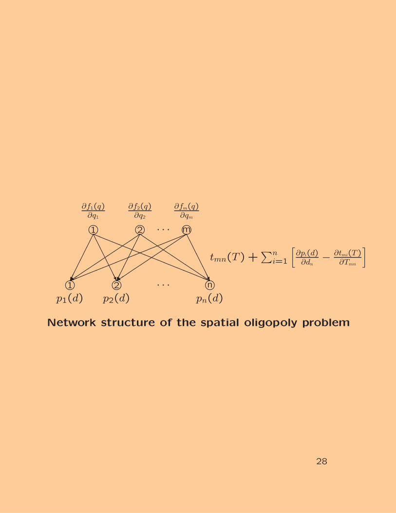
The underlying network structure of the model is de-

picted in Figure 2 with the cost on link (i, j) given by

tij(T) +∑n

l=1

[∂pl(d)

∂dj− ∂til(T )

∂Tij

]Til.

27

m m m

m m m

1 2 · · · n

1 2 · · · m

p1(d) p2(d) pn(d)

∂f1(q)∂q1

∂f2(q)∂q2

∂fm(q)∂qm

tmn(T) +∑n

i=1

[∂pi(d)

∂dn− ∂tmi(T )

∂Tmn

]��

��

��

���

AAAAAAAAU

aaaaaaaaaaaaaaaaaaa

��

��

��

��

���+

��

��

��

���

QQ

QQ

QQ

QQ

QQQ

AAAAAAAAU

��

��

��

��

���+

!!!!!!!!!!!!!!!!!!!

Network structure of the spatial oligopoly problem

28

Relationship Between Spatial Oligopolies andSpatial Price Equilibrium Problems

Consider now a spatial oligopoly model of the type justdiscussed but endowed with the following structure.

The m firms are grouped into J groups: S1, . . . , SJ, calledsupply markets with ma firms in supply market Sa, thatis,

∑Ja=1 ma = m and ∪J

a=1Sa = {1,2, . . . , m}. The firmsin supply market Sa ship to demand market j a shipmentQaj of the commodity given by

Qaj =∑i∈Sa

Tij, a = 1, . . . , J; j = 1, . . . , n. (32)

The total production sa of all firms in Sa is

sa =n∑

j=1

Qaj =∑i∈Sa

qi =n∑

j=1

∑i∈Sa

Tij. (33)

29

Assume that the supply markets represent geographiclocations and thus all firms belonging to the same supplymarket face identical production and transaction costs.This is expressed through the following assumptions:

(a). All firms in supply market Sa have the same pro-duction cost ga, that is,

fi = ga, if i ∈ Sa. (34)

(b). All firms in supply market Sa face the same trans-action cost caj to the demand market j, that is,

tij = caj, if i ∈ Sa. (35)

(c). The production cost of any firm in supply marketSa is determined solely by the production pattern, thatis,

g = g(s) (36)

where g and s are vectors in Rm with components ga andsa and g is a known smooth function.

(d). The transaction cost of any firm in a supply marketSa to the demand market j is determined solely by theshipment distribution

c = c(Q), (37)

where c and Q are J × n matrices with components caj

and Qaj and c is a known smooth function.

30

Finally, the demand price at any demand market maydepend, as in the general model, upon the commoditydemand pattern, namely,

p = p(d), (38)

where p and d are vectors in Rn with components pj anddj and p is a known smooth function.

In the present case if i ∈ Sa, we have by virtue of (34),(36), and (33),

∂fi

∂qi=

∑b

∂ga

∂sb

∂sb

∂qi=

∂ga

∂sa, .39)

and, due to (35), (37), and (32),

∂tij

∂Til

=∑b,γ

∂caj

∂Qbγ

∂Qbγ

∂Til

=∂caj

∂Qal

. (40)

Using (39), (33), (35), (32), and (40), we may nowwrite variational inequality (31) in the form:∑

a

∂ga(s∗)∂sa

(sa − s∗a) +∑aj

caj(Q∗) × (Qaj − Q∗

aj)

−∑

j

pj(d∗) × (dj − d∗

j)

−∑a,j,l

[∂pj(d∗)

∂dl

− ∂caj(Q∗)∂Qal

] ∑i∈Sa

T ∗ij(Til − T ∗

il) ≥ 0. (41)

31

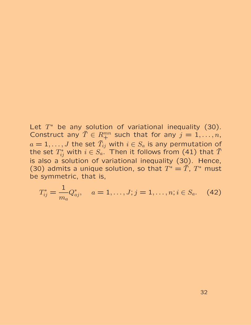
Let T ∗ be any solution of variational inequality (30).Construct any T̃ ∈ Rmn

+ such that for any j = 1, . . . , n,

a = 1, . . . , J the set T̃ij with i ∈ Sa is any permutation ofthe set T ∗

ij with i ∈ Sa. Then it follows from (41) that T̃

is also a solution of variational inequality (30). Hence,(30) admits a unique solution, so that T ∗ = T̃ , T ∗ mustbe symmetric, that is,

T ∗ij =

1

maQ∗

aj, a = 1, . . . , J; j = 1, . . . , n; i ∈ Sa. (42)

32

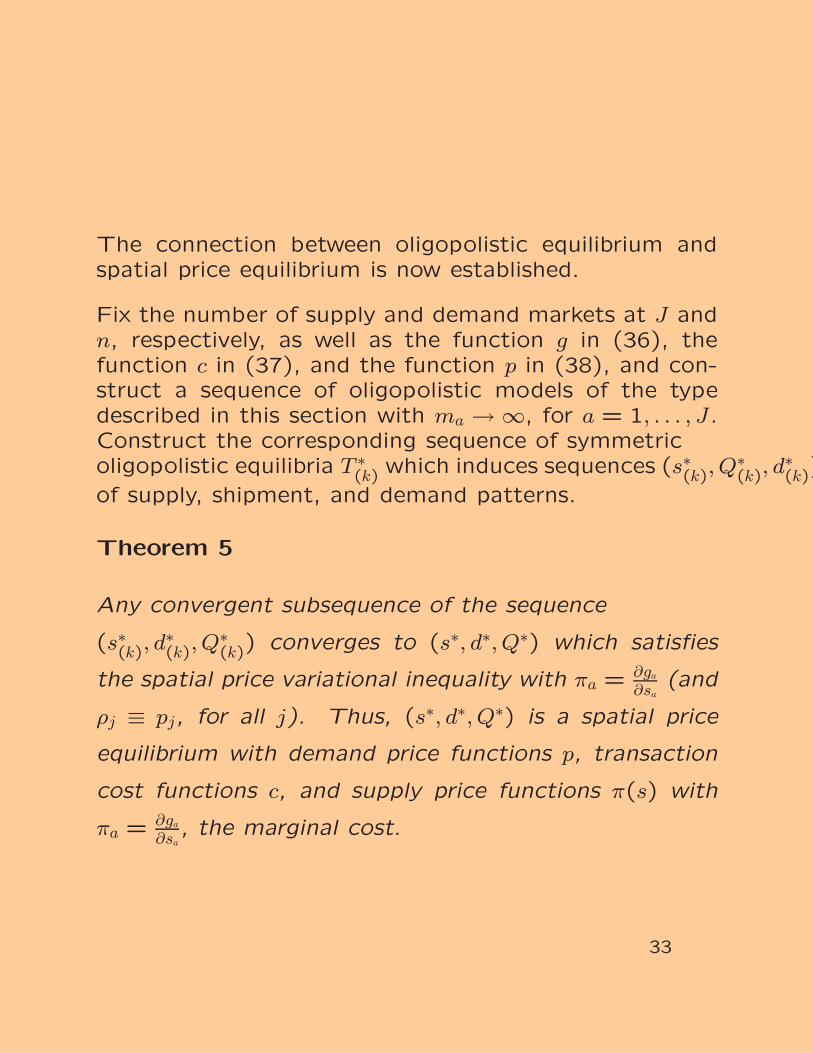
The connection between oligopolistic equilibrium andspatial price equilibrium is now established.

Fix the number of supply and demand markets at J andn, respectively, as well as the function g in (36), thefunction c in (37), and the function p in (38), and con-struct a sequence of oligopolistic models of the typedescribed in this section with ma → ∞, for a = 1, . . . , J.Construct the corresponding sequence of symmetricoligopolistic equilibria T ∗

(k) which induces sequences (s∗(k), Q∗(k), d

∗(k))

of supply, shipment, and demand patterns.

Theorem 5

Any convergent subsequence of the sequence

(s∗(k), d∗(k), Q

∗(k)) converges to (s∗, d∗, Q∗) which satisfies

the spatial price variational inequality with πa = ∂ga

∂sa(and

ρj ≡ pj, for all j). Thus, (s∗, d∗, Q∗) is a spatial price

equilibrium with demand price functions p, transaction

cost functions c, and supply price functions π(s) with

πa = ∂ga

∂sa, the marginal cost.

33

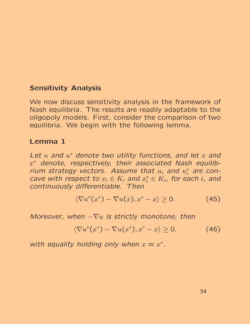
Sensitivity Analysis

We now discuss sensitivity analysis in the framework ofNash equilibria. The results are readily adaptable to theoligopoly models. First, consider the comparison of twoequilibria. We begin with the following lemma.

Lemma 1

Let u and u∗ denote two utility functions, and let x andx∗ denote, respectively, their associated Nash equilib-rium strategy vectors. Assume that ui and u∗

i are con-cave with respect to xi ∈ Ki and x∗

i ∈ Ki, for each i, andcontinuously differentiable. Then

〈∇u∗(x∗) −∇u(x), x∗ − x〉 ≥ 0. (45)

Moreover, when −∇u is strictly monotone, then

〈∇u∗(x∗) −∇u(x∗), x∗ − x〉 ≥ 0, (46)

with equality holding only when x = x∗.

34

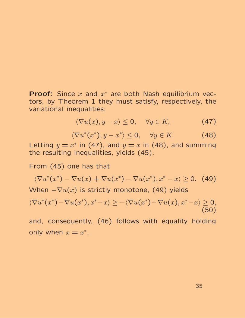
Proof: Since x and x∗ are both Nash equilibrium vec-tors, by Theorem 1 they must satisfy, respectively, thevariational inequalities:

〈∇u(x), y − x〉 ≤ 0, ∀y ∈ K, (47)

〈∇u∗(x∗), y − x∗〉 ≤ 0, ∀y ∈ K. (48)

Letting y = x∗ in (47), and y = x in (48), and summingthe resulting inequalities, yields (45).

From (45) one has that

〈∇u∗(x∗) −∇u(x) + ∇u(x∗) −∇u(x∗), x∗ − x〉 ≥ 0. (49)

When −∇u(x) is strictly monotone, (49) yields

〈∇u∗(x∗)−∇u(x∗), x∗−x〉 ≥ −〈∇u(x∗)−∇u(x), x∗−x〉 ≥ 0,(50)

and, consequently, (46) follows with equality holding

only when x = x∗.

35

We now present another result.

Theorem 6

Let u and u∗ denote two utility functions, and x andx∗ the corresponding Nash equilibrium strategy vectors.Assume that ∇u satisfies the strong monotonicity as-sumption

〈∇u(x) −∇u(y), x − y〉 ≤ −α‖x − y‖2, ∀x, y ∈ K, (51)

where α > 0. Then

‖x∗ − x‖ ≤ 1

α‖∇u∗(x∗) −∇u(x∗)‖. (52)

Proof: From Lemma 1 one has that (45) holds andfrom (45) one has that

〈∇u∗(x∗) −∇u(x) + ∇u(x∗) −∇u(x∗), x∗ − x〉 ≥ 0. (53)

But from the strong monotonicity condition (51), (53)yields

〈∇u∗(x∗) −∇u(x∗), x∗ − x〉 ≥ −〈∇u(x∗) −∇u(x), x∗ − x〉

≥ α‖x∗ − x‖2. (54)

By virtue of the Schwartz inequality, (54) yields

α‖x∗ − x‖2 ≤ ‖∇u∗(x∗) −∇u(x∗)‖‖x∗ − x‖ (55)

from which (52) follows and the proof is complete.

36

Below are references cited in the lecture as well as ad-ditional supplementary ones.

References

Cournot, A. A., Researches into the MathematicalPrinciples of the Theory of Wealth, 1838, Englishtranslation, MacMillan, London, England, 1897.

Dafermos, S., “An iterative scheme for variational in-equalities,” Mathematical Programming 26 (1983) 40-47.

Dafermos, S., and Nagurney, A., “Oligopolistic and com-petitive behavior of spatially separated markets,” Re-gional Science and Urban Economics 17 (1987) 245-254.

Flam, S. P., and Ben-Israel, A., “A continuous ap-proach to oligopolistic market equilibrium,” OperationsResearch 38 (1990) 1045-1051.

Friedman, J., Oligopoly and the Theory of Games,North-Holland, Amsterdam, The Netherlands, 1977.

Gabay, D., and Moulin, H., “On the uniqueness and

stability of Nash-equilibria in noncooperative games,”

in Applied Stochastic Control in Econometrics and

Management Science, pp. 271-294, A. Bensoussan,

P. Kleindorfer, and C. S. Tapiero, editors, North-Holland,

Amsterdam, The Netherlands, 1980.

37

Gabzewicz, J., and Vial, J. P., “Oligopoly ‘a la Cournot’in a general equilibrium analysis,” Journal of EconomicTheory 14 (1972) 381-400.

Harker, P. T., “A variational inequality approach frorthe determination of oligopolistic market equilibrium,”Mathematical Programming 30 (1984) 105-111.

Harker, P. T., “Alternative models of spatial competi-tion,” Operations Research 34 (1986) 410-425.

Hartman, P., and Stampacchia, G., “On some nonlinearelliptic differential functional equations,” Acta Mathe-matica 115 (1966) 271-310.

Haurie, A., and Marcotte, P., “On the relationship be-tween Nash-Cournot and Wardrop equilibria,” Networks15 (1985) 295-308.

Karamardian, S., “Nonlinear complementarity problemwith applications, ” Journal of Optimization Theory andApplications 4 (1969), Part I, 87-98, Part II, 167-181.

Manas, M., “A linear oligopoly game,” Econometrica

40 (1972) 917-922.

38

Mas-Colell, A., “Walrasian equilibria, Part I: Mixed strate-gies,” Journal of Economic Theory 30 (1983) 153-170.

Murphy, F.H., Sherali, H. D., and Soyster, A. L., “Amathematical programming approach for determiningoligopolistic market equilibrium,” Mathematical Program-ming 24 (1982) 92-106.

Nagurney, A., “Algorithms for oligopolistic market equi-librium problems,” Regional Science and Urban Eco-nomics 18 (1988) 425-445.

Nash, J. F., “Equilibrium points in n-person games,”Proceedings of the National Academy of Sciences, USA36 (1950) 48-49.

Nash, J. F., “Noncooperative games,” Annals of Math-ematics 54 (1951) 286-298.

Novshek, W., “Cournot equilibrium with free entry,” Re-view of Economic Studies 47 (1980) 473-486.

Novshek, W., and Sonnenschein, H., “Walrasian equi-

libria as limits of noncooperative equilibria, Part II, Pure

strategies,” Journal of Economic Theory 30 (1983)

171-187.

39

Okuguchi, K., Expectations and Stability in OligopolyModels, Lecture Notes in Economics and MathematicalSystems 138, Springer-Verlag, Berlin, Germany, 1976.

Okuguchi, K., and Szidarovsky, F., The Theory of O-ligopoly with Multi - Product Firms, Lecture Notesin Economics and Mathematical Systems 342, Springer-Verlag, Berlin, Germany, 1990.

Qiu Y., “Solution properties of oligopolistic networkequilibria,” Networks 71 (1991) 565-580.

Rosen, J. B., “Existence and uniqueness of equilibriumpoints for concave n-person games,” Econometrica 33(1965) 520-533.

Spence, M., “The implicit maximization of a functionin monopsolistically competitive markets,” Harvard In-stitute of Economic Research, Harvard University Dis-cussion Paper 461 (1976).

Szidarovsky, F., and Yakowitz, S., “A new proof of theexistence and uniqueness of the Cournot equilibrium, ”International Economic Review 18 (1977) 787-789.

Tobin, R. L., “Sensitivity analysis for a Cournot equilib-

rium,” Operations Research Letters 9 (1990) 345-351.

40