Old Keynesian Economics∗

Roger E. A. Farmer†

UCLA, Dept. of Economics

September 21, 2006

Abstract

I provide an outline of how a modern theory of search, modelled bya two-sided matching function, can be used to form a microfoundationto Keynesian economics. This search theory of the labor market hasone less equation than unknown and, when combined with the idea thatinvestment is driven exogenously by ‘animal spirits,’ the marriage leadsto a microfounded theory of business cycles. This alternative theoryhas very different implications from the standard interpretations ofKeynes that has become enshrined in new-Keynesian economics. I callthe alternative, ‘old-Keynesian economics’ and I show that it leads toa model with multiple belief driven steady states.

1 Keynes and the Keynesians

In his (1966) book, On Keynesian Economics and the Economics of Keynes,Axel Leijonhufvud made the distinction between the economics of the Gen-eral Theory (Keynes 1936) and the interpretation of Keynesian economicsby Hicks and Hansen that was incorporated into the IS-LM model and thatforms the basis for new-Keynesian economics. In that book, he pointed outthat although the new-Keynesians give a central role to the assumption ofsticky prices, the sticky-price assumption is a part of the mythology of Key-nesian economics that is inessential to the main themes of the General The-ory. In this paper I will sketch an alternative microfoundation to Keynesian

∗This paper was prepared for a Conference in honor of Axel Leijonhufvud held atUCLA on August 30th - 31st 2006. Although I am certain that Axel will not agree witheverything that I say in this essay, I hope that he will recognize a trace of the Leijonhufvudinfluence creeping through the pages.

†This research was supported by NSF award SES 0418074.

1

economics that formalizes this argument by providing a microfoundationthat does not rely on sticky prices. I call this alternative microfoundation,old-Keynesian economics.

It is fitting that this paper should appear in a volume in honor of AxelLeijonhufvud since the ideas I will describe owe much to his influence. Al-though Axel’s thesis was written at Northwestern University, his work onKeynes came to fruition at UCLA; the location of his first academic appoint-ment. In the 1960’s, UCLA had developed a healthy tradition of tolerancefor non mainstream ideas and, as the beneficiary of that same atmosphereof tolerance, it is a privilege to be able to use this occasion to acknowledgethe debt that I owe to Axel as both a mentor and a friend.

In the following paragraphs, I will describe a plan to embed a versionof search theory into a general equilibrium model in a way that provides amicrofoundation to the economics of the General Theory. Since UCLA hasa some claim to be the birthplace of search theory (with the work of ArmenAlchian (1970) and John McCall (1970)), this project is the continuation ofa rich UCLA tradition in more ways than one.

Whereas Keynes argued that the general level of economic activity isdetermined in equilibrium by aggregate demand, this idea is not present innew-Keynesian economics which views unemployment as a short-run phe-nomenon that arises when prices are temporarily away from their long-runequilibrium levels. Since the appearance of the work of Edmund Phelps(1970) and Milton Friedman (1968) the concept of demand failure as apurely temporary phenomenon has been enshrined in the concept of thenatural rate of unemployment and although the natural rate hypothesis hasbecome a central part of all of modern macroeconomics it is not a compo-nent of the theory I will develop here. As a consequence the welfare andpolicy implications of old and new-Keynesian economics are very different.

I begin, in Section 2, by sketching a simple one period model that cap-tures the essence of my argument. The idea is to model the process of mov-ing workers from unemployment to employment with a neoclassical searchtechnology of the kind introduced to the literature by Phelps (1968). Iwill argue that this technology cannot easily be decentralized because moralhazard prevents the creation of markets for the search inputs. Instead, Iwill introduce a market in which workers post wages in advance and I willassume that all workers post the same wage. This leads to a model withone less equation than unknown since the two markets for search inputsmust be cleared by a single price. This underdetermined labor market isa perfect match for a Keynesian theory of demand determination in whichthe quantity of output produced and the volume of labor employed is deter-

2

mined by aggregate demand. I call this a demand constrained equilibrium.In Section 3 I provide a sketch of how the equilibrium concept of a demandconstrained equilibrium can be extended to a full-blown dynamic stochasticgeneral equilibrium model.

2 A One Period Model

This section describes my main idea. Its purpose is to lay out a simpleenvironment in which one can compare the socially efficient allocation ofresources to the allocation that occurs in a decentralized equilibrium. Inmore sophisticated versions of the theory, described in Section 3, I introduceinvestment as a key determinant of demand. In the current section, alleconomic activity takes place in a single period. In this one-period model,government purchases take the place of investment spending as an exogenousdeterminant of the level of economic activity. Although this environmentabstracts from many important elements of the real world it is rich enough tocapture the basic idea; that a modified search-theoretic-model (MS-model)leads to inefficient equilibria because of a missing market.

2.1 The economic environment

Consider a one-period model with a large number of workers and firms.Firms produce output using a constant-returns-to-scale technology in whichlabor is the sole input. Labor is transferred from households to firms usinga convex matching technology with unemployment and vacancies as inputs.

There is a unit measure of entrepreneurs each of whom runs a firm. Eachentrepreneur has access to a technology that produces output Y from laborinput L:

Y = AL (1)

where A > 0 is the marginal product of an extra unit of labor input. En-trepreneurs are identical and, the symbols Y and L refer interchangeablyto average aggregate variables and to individual variables. The utility ofthe entrepreneur is captured by a continuous increasing concave functionJE¡XE

¢, where

XE = CE − V (2)

is the sum of the entrepreneur’s consumption CE , and V measures the disu-tility of posting vacancies. The cost of vacancies is measured in consumptionunits.

3

In addition to the mass of entrepreneurs there is a continuum of workerswith preferences JW

¡CW

¢where JW is a concave increasing utility function

and CW is workers’ consumption. Each worker supplies one unit of effortinelastically to a constant-returns-to-scale matching technology:

m = BUθV 1−θ (3)

where m is the measure of workers that find jobs when U unemployed work-ers search for jobs and V vacancies are posted by entrepreneurs. B is ascaling parameter. Since U = 1 (all workers are initially unemployed) thisreduces to the expression

m = BV 1−θ. (4)

In a dynamic model, employment will appear as a state variable in aprogramming problem since it takes time to recruit new workers. In thissection, I abstract from this aspect of labor market dynamics by assumingthat all workers must be recruited in the current period. This assumptionimplies that employment, equal to the number of matches, is represented bythe equation:

L = m. (5)

This completes a description of preferences and technology. Next I turn tothe problem solved by a benevolent social planner whose goal is to maximizea weighted sum of the utilities of the two agents.

2.2 The social planning problem

The social planner faces the following problem:

maxλJW¡CW

¢+ (1− λ)JE

¡CE − V

¢(6)

such thatL = BV 1−θ (7)

CE +CW ≤ AL. (8)

This problem has the following solution for the optimal quantity of employ-ment, L∗

L∗ = B1θ (A (1− θ))

1−θθ . (9)

Since workers do not receive disutility from work, all unemployed workerssearch all of the time. Entrepreneurs do not like to search and optimalemployment balances the disutility of search against increased output fromgreater employment.

4

In the planning optimum, employment depends on three parameters, A,B and θ. A measures the productivity of the production technology andB the productivity of the search technology. If either of these parametersincreases, search effort becomes more productive and the social planner willchoose more of it. A decrease in θ also makes the search of the entrepreneurmore productive and has the same qualitative effect as an increase in B.

The allocation of output between workers and entrepreneurs is deter-mined by the parameter λ which is a number between 0 and 1 that representsthe weight placed by the planner on the worker in social utility.

2.3 A decentralized solution

In order to discuss the role of government policy, in this section I will adda government to the model that taxes output with a proportional tax τand purchases commodities G. I will assume that commodities purchasedby government do not directly yield utility in order to make the point thatapparently socially inefficient government expenditure can be Pareto im-proving.

Since the environment I have described satisfies all the desiderata of thewelfare theorems, standard results from general equilibrium theory implythat the social planning solution could be decentralized by a complete setof competitive markets. To achieve this decentralization one would need totreat the matching technology in the same way as the production functionand to assume the existence of a set of profit maximizing employment agen-cies that purchases, from workers the exclusive right to be matched withan entrepreneur and from entrepreneurs, the exclusive right to be matchedwith a worker. There are good reasons why these markets do not exist;for example, an unemployed worker could easily cheat and sign employmentcontracts with multiple agencies. On being matched, the worker would havean incentive to claim incompatibility with the employer and to continuebeing paid for further search activity.

Consider instead the following decentralized environment which is basedon the idea of a competitive search equilibrium due to Espen Moen (1997). Inthis environment, firms post wages in advance and, in equilibrium, all firmspost the same wage. Firms and workers meet randomly and on meeting,the entrepreneur and worker form a matched pair and produce output usingthe technology described by Equation (1). The worker receives wage incomefrom the match and the entrepreneur receives profit Π where:

Π = AL− ωL. (10)

5

The worker and the firm take the numbers pu and pv as given. pu is theprobability a worker receives a job and pv is the measure of workers hiredby an entrepreneur that posts 1 vacancy. Later, I will describe how thesevariables are determined in equilibrium. Each worker secures a job withprobability pu. The worker is paid an after tax wage which he spends onconsumption CW . Each entrepreneur posts V vacancies and hires a measureof workers of size V pv. Each vacancy posted yields one unit of disutility.

The worker’s problem is trivial since he needs only to search for a joband to spend his after-tax income on consumption. The utility maximizingentrepreneur will choose V,L and CE to solve the problem,

max JE¡CE − V

¢(11)

such thatCE ≤ Π (1− τ) (12)

Π = AL− ωL (13)

L = pvV (14)

where the rate of tax on profit is the same as the rate on labor income. Thesolution to the entrepreneur’s problem is given by the correspondence:

V =

⎧⎨⎩∞ if (A− ω) pv (1− τ) > 1[0,∞] if (A− ω) pv (1− τ) = 10 if (A− ω) pv (1− τ) < 1.

(15)

Government chooses a tax rate τ and a level of purchases G.

2.4 The equilibrium concept

This section introduces my equilibrium concept. To describe it, I have appro-priated a term, demand constrained equilibrium, that was used in a literatureon general equilibrium with fixed prices that evolved in the 1970’s from thework of Jean Pascal Benassy (1975), Jacques Dreze (1975) and EdmondMalinvaud (1977). Although fixed-price models with rationing of the kindstudied by these authors are sometimes called demand constrained equilib-ria; that is not what I mean here. Instead I will use the term to refer to acompetitive search model that is closed with a materials balance condition.The common heritage of both usages of demand constrained equilibrium isthe idea of effective demand from Keynes’ General Theory.

6

Definition 1 (Demand Constrained Equilibrium) For any given τ and Ga demand constrained equilibrium (DCE) is a real wage ω, an allocation{CW , CE, V, L} and a pair of matching probabilities, pu and pv, with thefollowing properties.1) Feasibility:

CE +CW ≤ AL (16)

L ≤ BV 1−θ (17)

G ≤ (1− τ)AL. (18)

2) Consistency with optimal choice:

V =

⎧⎨⎩∞ if (A− ω) pv (1− τ) > 1[0,∞] if (A− ω) pv (1− τ) = 10 if (A− ω) pv (1− τ) < 1.

(19)

3) Consistency of matching probabilities:

pu = L (20)

pv =L

V. (21)

Property 3) needs some explanation. The probability of contacting apartner is determined by how many others are searching. Let V̄ represent theaverage number of vacancies posted by entrepreneurs and let L̄ represent theaggregate number of successful matches (equal to aggregate employment).The probability that a worker finds a job, and the measure of workers hiredby an entrepreneur who posts V vacancies, are determined by the conditions

pu = L̄, pv =L̄

V̄. (22)

In a symmetric equilibrium, the search intensities must be the same acrossagents and hence

V = V̄ , L = L̄. (23)

7

2.5 The Keynesian cross

In modern DSGE models the government is assumed to choose expenditureand taxes subject to a constraint. Models that incorporate a constraint ofthis kind were dubbed Ricardian by Robert Barro (1974). But in modelswith multiple equilibria there is no reason to impose a government budgetconstraint and Eric Leeper (1991), discussing models of monetary and fiscalpolicy, has argued that one should allow government to choose both taxesand expenditure and that this choice selects an equilibrium. He calls a policyin which the government choose both taxes and expenditure, an ‘activefiscal regime.’ The modified-search model of the labor market is one withmultiple equilibria and hence, one can close the model in the way advocatedby Leeper.

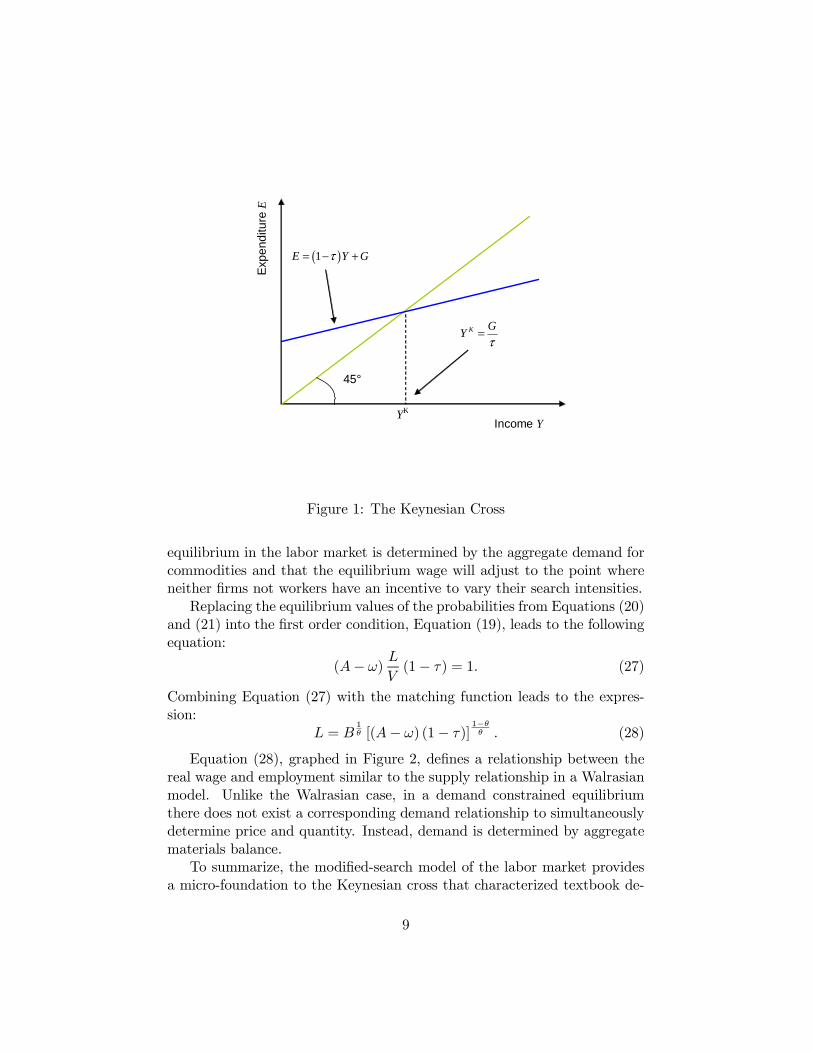
In textbook descriptions of simple Keynesian models, equilibrium is typ-ically described by the diagram pictured in Figure 1. The 45 degree line inthis diagram is a supply curve, representing the assumption that whatever isdemanded will be supplied. The second upward sloping line is a Keynesiandemand curve obtained by combining the equations

Y = C +G, (24)

C = (1− τ)Y, (25)

to yield the equilibrium condition

Y =G

τ. (26)

It is precisely this pair of equations that determine determine equilibriumoutput in the current model.

The central difficulty faced by old Keynesian economics was that theKeynesian model as expounded by John Hicks and Alvin Hansen had nomicrofoundation. They could not answer the question: Why doesn’t thereal wage fall to establish equilibrium in the labor market? The answerI propose to that question is that there is a missing market. A completedecentralization of the search process as a competitive equilibrium wouldrequire a market for vacancies and a separate market for the search timeof entrepreneurs. In practice there is a single competitive search market inwhich competition forces all firms to post the same wage.

2.6 Determining the equilibrium wage

Standard competitive theory does not have a good explanation of the processby which an equilibrium is established. Nor will I. Instead, I will argue that

8

Income Y

Exp

endi

ture

E

45°

( )1E Y Gτ= − +

YK

K GY

τ=

Figure 1: The Keynesian Cross

equilibrium in the labor market is determined by the aggregate demand forcommodities and that the equilibrium wage will adjust to the point whereneither firms not workers have an incentive to vary their search intensities.

Replacing the equilibrium values of the probabilities from Equations (20)and (21) into the first order condition, Equation (19), leads to the followingequation:

(A− ω)L

V(1− τ) = 1. (27)

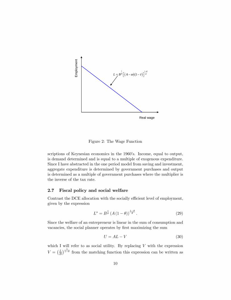
Combining Equation (27) with the matching function leads to the expres-sion:

L = B1θ [(A− ω) (1− τ)]

1−θθ . (28)

Equation (28), graphed in Figure 2, defines a relationship between thereal wage and employment similar to the supply relationship in a Walrasianmodel. Unlike the Walrasian case, in a demand constrained equilibriumthere does not exist a corresponding demand relationship to simultaneouslydetermine price and quantity. Instead, demand is determined by aggregatematerials balance.

To summarize, the modified-search model of the labor market providesa micro-foundation to the Keynesian cross that characterized textbook de-

9

Real wage

Em

ploy

men

t ( )( )

1 1

1L B Aθ

θ θω τ−

⎡ ⎤= − −⎣ ⎦

Figure 2: The Wage Function

scriptions of Keynesian economics in the 1960’s. Income, equal to output,is demand determined and is equal to a multiple of exogenous expenditure.Since I have abstracted in the one period model from saving and investment,aggregate expenditure is determined by government purchases and outputis determined as a multiple of government purchases where the multiplier isthe inverse of the tax rate.

2.7 Fiscal policy and social welfare

Contrast the DCE allocation with the socially efficient level of employment,given by the expression

L∗ = B1θ (A (1− θ))

1−θθ . (29)

Since the welfare of an entrepreneur is linear in the sum of consumption andvacancies, the social planner operates by first maximizing the sum

U = AL− V (30)

which I will refer to as social utility. By replacing V with the expression

V =¡LB

¢ 11−θ from the matching function this expression can be written as

10

a function of L,

U = AL−µL

B

¶ 11−θ

. (31)

Given the maximal value of U , the social planner distributes consumptionacross entrepreneurs and workers to maximize a weighted sum of individualutilities. Notice that the maximization of social utility leads to the expres-sion given in Eq (29).

Employment L

Soc

ial U

tility

U

( )f τ

*L

( ),U G τ

( )0f

KL

K G

LAτ

=

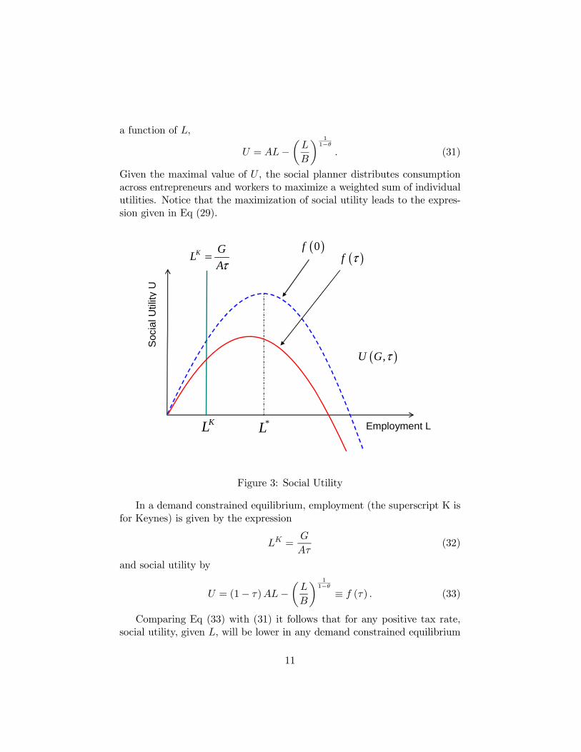
Figure 3: Social Utility

In a demand constrained equilibrium, employment (the superscript K isfor Keynes) is given by the expression

LK =G

Aτ(32)

and social utility by

U = (1− τ)AL−µL

B

¶ 11−θ≡ f (τ) . (33)

Comparing Eq (33) with (31) it follows that for any positive tax rate,social utility, given L, will be lower in any demand constrained equilibrium

11

with positive taxes, reflecting the fact that government purchases are as-sumed to yield no utility. The set of possible demand constrained equilibriais depicted in Figure 3. The curves f (0) and f (τ) represent attainable levelsof adjusted social utility (the right side of Eq. (33)) for different tax rates.

For a given tax rate, employment increases as government purchasesincrease. In the figure this would correspond to shifting the line LK to theright. As G increases, social utility will increase up until a maximum thatdepends on τ . At that point further increases in government purchases willincrease employment but decrease welfare. It follows that the optimal policyis approached (but never achieved) by lowering the tax rate towards zeroand choosing G to pick LK = L∗.

3 An Intertemporal Model

My purpose in this section is to provide a brief sketch of how one mightdevelop the static model, described above, into a full blown dynamic sto-chastic general equilibrium model. The work I will describe is in progressand will be reported in more detail elsewhere. There are nevertheless severalimportant details of the generalization that are worth describing and alsosome preliminary results that may be of interest.

The equilibrium I will use is a generalization of the static concept ofdemand constrained equilibrium. Since the factor markets are incomplete,I will close the model by assuming that investment expenditure depends onthe self-fulfilling beliefs of entrepreneurs. The result is a model with multiplestationary equilibria, indexed by beliefs.

3.1 Recursive utility and the real interest rate

The conventional approach to dynamic general equilibrium posits the exis-tence of a representative agent with time additively separable preferences.This approach restricts the long-run real interest rate to equal a paramet-rically determined rate of time preference and it is too restrictive for mypurposes. Since I will be concerned with the role of fiscal policy I willneed to describe a model in which aggregate expenditure is a function ofthe real interest rate. If this is fixed by the time preference rate, govern-ment purchases will “crowd out” private consumption and have no effect onequilibrium employment in the long run. For this reason, I chose to modelpreferences with a recursive utility function of the kind studied by Uzawa(1968), Lucas and Stokey (1984) and Epstein and Hynes (1983) and adaptedby Farmer-Lahiri (2005) to allow for balanced growth.

12

Recursive utility functions allow the long-run real rate of interest todepend on consumption sequences. An alternative model with this propertyis a version of the overlapping generations model with long lived agents.I will not follow this approach here since empirically plausible versions ofthe overlapping generations model are more complicated than the recursiverepresentative agent approach.

Utility is defined by the equation,

Jt = At

∞Xt=1

E1

"−ρt1

µAt

Ct

¶λ#

(34)

wherep11 = 1 (35)

ρt1 = βt−1tY

s=2

µAs

As−1

¶µAs−1Cs−1

¶λ

, t > 1. (36)

The term At is an exogenous trend that grows at the rate of growthof the economy and β and λ are parameters. These preferences allow therepresentative agent’s discount rate to depend on consumption relative to agrowing trend. The inclusion of a trend in preferences is necessary for thisrepresentation to be consistent with balanced growth and it could potentiallyarise from a more fundamental assumption in which one assumes a homeproduction sector (as in Benhabib, Rogerson andWright (1991)) where homeproductivity grows at the same rate as productivity in the market sector.

3.2 Some details of the model

The representative agent is situated in a relatively standard one-sector growthmodel with the additional twist that there is a matching technology for mov-ing labor from households to firms. This technology implies that labor inplace at firms in period t is given by the expression

Lt = Lt−1 (1− s) +B (1− Lt)θ V 1−θt (37)

where s represents exogenous separations, the second expression on the righthand side of Eq (37) represents matches at date t and 1−Lt is the fraction ofthe labor force unemployed. The timing of the matching function is chosento enable demand shocks to influence output contemporaneously — that is,workers can produce in the period in which they are employed.

Output is produced with the technology

Yt = Kαt (AtXt)

1−α (38)

13

where Xt is labor used in productive activity and it is related to Lt (totallabor in place at the firm) and Vt (labor used in recruiting) by the expression,

Vt +Xt = Lt. (39)

Other elements of the model are standard. The representative agent inelas-tically supplies a unit measure of labor to the market and at any given dateUt units of labor are unemployed and Lt are employed where Ut = 1− Lt.

I will assume that agents are able to trade a complete set of contingentclaims and that fundamental uncertainty is indexed by histories of eventsthat I will denote σt. Thus, σt is a list of everything relevant to the economythat occurred up to and including date t. The agent faces a sequence of realwages and interest rates and chooses consumption sequences to maximizeexpected utility subject to a sequence of budget constraints

Kt+1 = Kt (1− δ) + ωtLt +Πt −Ct (40)

limT→∞

QT1

¡σT¢KT+1

¡σT¢ ≥ 0 (41)

where Πt is profit, ωt is the real wage and QT1

¡σT¢is the present value price

of capital at date T in event history σT .

3.3 A definition of equilibrium

The following definition is a sketch of how the DCE concept can be extendedto a DSGE model.

Definition 2 For a given sequence {It} a Demand Constrained Equilibrium(DCE) is a 4-tuple of quantity sequences

©Ct

¡σt¢, Vt

¡σt¢, Lt (σt) ,Kt+1

¡σt¢ª

(as functions of event histories), a sequence of matching probabilities©pv¡σt¢ª,

a sequence of rental rates and wage rates©qt¡σt¢, ω¡σt¢ª, and a sequence

of utility levels and profits©J¡σt¢,Π¡σt¢ª, with the following properties:

1) Taking as given the sequences of rental rates, wage rates and matchingprobabilities the quantity sequences maximize the expected net present valueof the firm.

2) Taking as given the sequences of rental rates and wage rates and the profitsequence the quantity sequences maximize the expected utility of the house-holds.

3) The matching probabilities are determined in equilibrium by equality of av-erage and agent specific unemployment and vacancy rates and the demandsand supplies for all commodities are equal.

14

3.4 Comparing an equilibrium with a planning optimum

Given the model outline sketched above one can show that, given certainbounds on investment sequences, there exists a different demand constrainedequilibrium for every stationary investment sequence. One can also establishthe existence of a unique balanced growth path that characterizes a station-ary planning optimum. Both concepts are characterized by the following setof seven equations in the eight variables jt,ct,kt,yt,it,Lt,Xt and Vt. Lowercase letters represent the ratio of variables to the trend growth path andγ = At

At−1 is the trend growth factor.

jt = Et

½(−1 + βγjt+1)

1

cλt

¾(42)

kt+1 =1− δ

γkt +

1

γyt − 1

γct (43)

yt = kαt (Xt)1−α (44)

yt = it + ct (45)

Xt = Lt − Vt (46)

Lt = (1− s)Lt−1 +B (1− Lt)θ V 1−θt (47)

1

ct= Et

(µ1

ct

¶λµjt+1jt

¶β

ct+1

µ1− δ +

yt+1kt+1

¶). (48)

A social planning optimum is defined by the previous seven equations andthe additional condition

1

ct

∙(1− α) yt

Xtg1 (Lt, Lt−1)+ (49)

Et

(µ1

ct

¶λµjt+1jt

¶γβ

ct+1

(1− α) yt+1Xt+1

g2 (Lt+1, Lt)

)#= 0.

where g (Lt, Lt−1) is a function that describes the relationship between Xt

(labor used to produce output) and the stocks of labor at the firm at datest and t− 1. One can show that a demand constrained equilibrium is deter-mined by the same seven equations (42) — (48) but the system is closed bythe assumption that investment follows the following exogenous stochasticprocess

it = iχt et (50)

15

where χ is parameter that measures persistence of the exogenous investmentsequence and et is a stochastic innovation to beliefs.

It is worth pausing at this point to draw attention to Equation (50) sinceit is the main feature that makes this a model of old-Keynesian economics.The term it is defined as the ratio of investment to a growing trend andthis equation states that investment evolves exogenously with no regard forexpected future profits. It is precisely this idea which I take to be central totheGeneral Theory and which has disappeared from much of modern macro-economics. Although my own previous work with Jess Benhabib (1994) andJang-Ting Guo (1994) went part way to rehabilitating animal spirits; in thatwork we only considered a model with a unique steady state. The currentproposal goes far beyond the previous literature since I am proposing toallow the steady state of the economy itself to be influenced by beliefs. Asin my previous work, all of these belief driven equilibria are fully rationaland leave no room for arbitrage opportunities or for mistaken expectations.

To explain the behavior of prices and matching probabilities in a beliefdriven equilibrium one can derive a separate set of equations that describeshow the rental rate qt, the real wage rate ωt and the match probability pvtdepend on the state. The real wage, for example, follows the process

ωt = (1− α)ytXt

µ1− 1

pvt

¶+Et

½γQt+1

t (1− α)yt+1Xt+1

(1− s)

pvt+1

¾= 0 (51)

where

pvt =Lt − (1− s)Lt−1

Lt −Xt. (52)

3.5 Some preliminary results

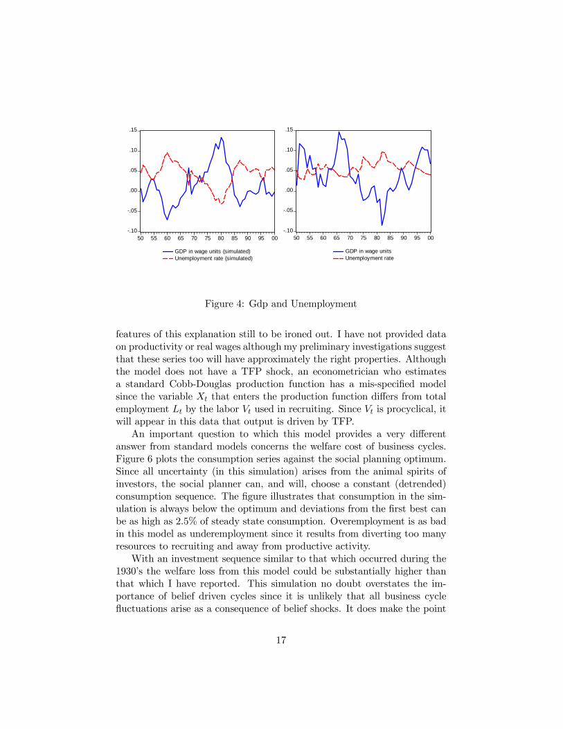
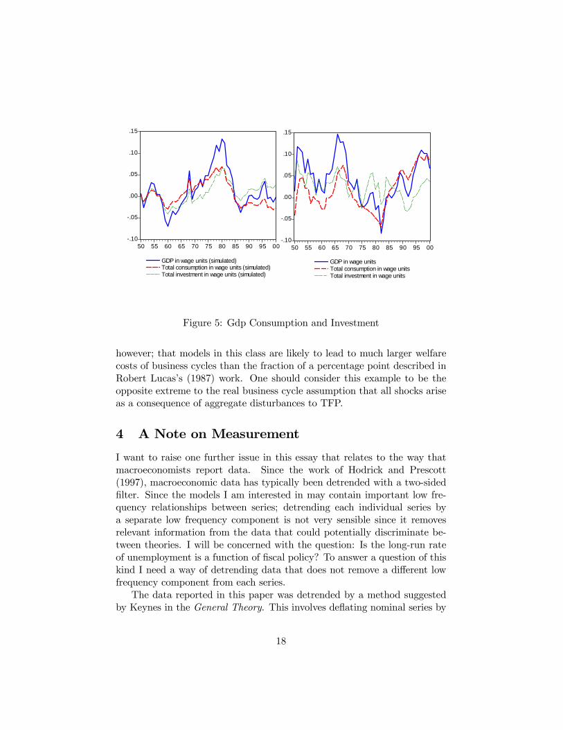
As a preliminary check on the chances of this model to fit data I simulated ademand constrained equilibrium for an investment sequence calibrated fit tothe properties of time series data; for this purpose I chose the shock to havea standard deviation of 0.04 and the autocorrelation parameter to equal 0.5.Figure 4 compares the properties of a single simulated data series (left panel)with the US data (right panel) for GDP and unemployment and Figure 5does the same for GDP, investment and consumption. In all cases the datawas detrended in the manner described in Section 4.

The exercise that I carried out to simulate these data series was similar tothat which characterizes many real business cycle papers. But the shock thatis driving the model is entirely driven by demand. Of course there are many

16

-.10

-.05

.00

.05

.10

.15

50 55 60 65 70 75 80 85 90 95 00

GDP in wage units (simulated)Unemployment rate (simulated)

-.10

-.05

.00

.05

.10

.15

50 55 60 65 70 75 80 85 90 95 00

GDP in wage unitsUnemployment rate

Figure 4: Gdp and Unemployment

features of this explanation still to be ironed out. I have not provided dataon productivity or real wages although my preliminary investigations suggestthat these series too will have approximately the right properties. Althoughthe model does not have a TFP shock, an econometrician who estimatesa standard Cobb-Douglas production function has a mis-specified modelsince the variable Xt that enters the production function differs from totalemployment Lt by the labor Vt used in recruiting. Since Vt is procyclical, itwill appear in this data that output is driven by TFP.

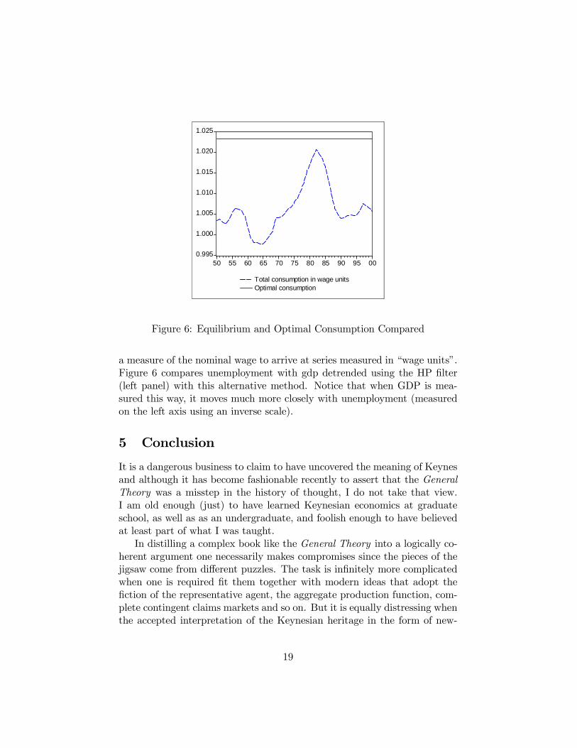
An important question to which this model provides a very differentanswer from standard models concerns the welfare cost of business cycles.Figure 6 plots the consumption series against the social planning optimum.Since all uncertainty (in this simulation) arises from the animal spirits ofinvestors, the social planner can, and will, choose a constant (detrended)consumption sequence. The figure illustrates that consumption in the sim-ulation is always below the optimum and deviations from the first best canbe as high as 2.5% of steady state consumption. Overemployment is as badin this model as underemployment since it results from diverting too manyresources to recruiting and away from productive activity.

With an investment sequence similar to that which occurred during the1930’s the welfare loss from this model could be substantially higher thanthat which I have reported. This simulation no doubt overstates the im-portance of belief driven cycles since it is unlikely that all business cyclefluctuations arise as a consequence of belief shocks. It does make the point

17

-.10

-.05

.00

.05

.10

.15

50 55 60 65 70 75 80 85 90 95 00

GDP in wage units (simulated)Total consumption in wage units (simulated)Total investment in wage units (simulated)

-.10

-.05

.00

.05

.10

.15

50 55 60 65 70 75 80 85 90 95 00

GDP in wage unitsTotal consumption in wage unitsTotal investment in wage units

Figure 5: Gdp Consumption and Investment

however; that models in this class are likely to lead to much larger welfarecosts of business cycles than the fraction of a percentage point described inRobert Lucas’s (1987) work. One should consider this example to be theopposite extreme to the real business cycle assumption that all shocks ariseas a consequence of aggregate disturbances to TFP.

4 A Note on Measurement

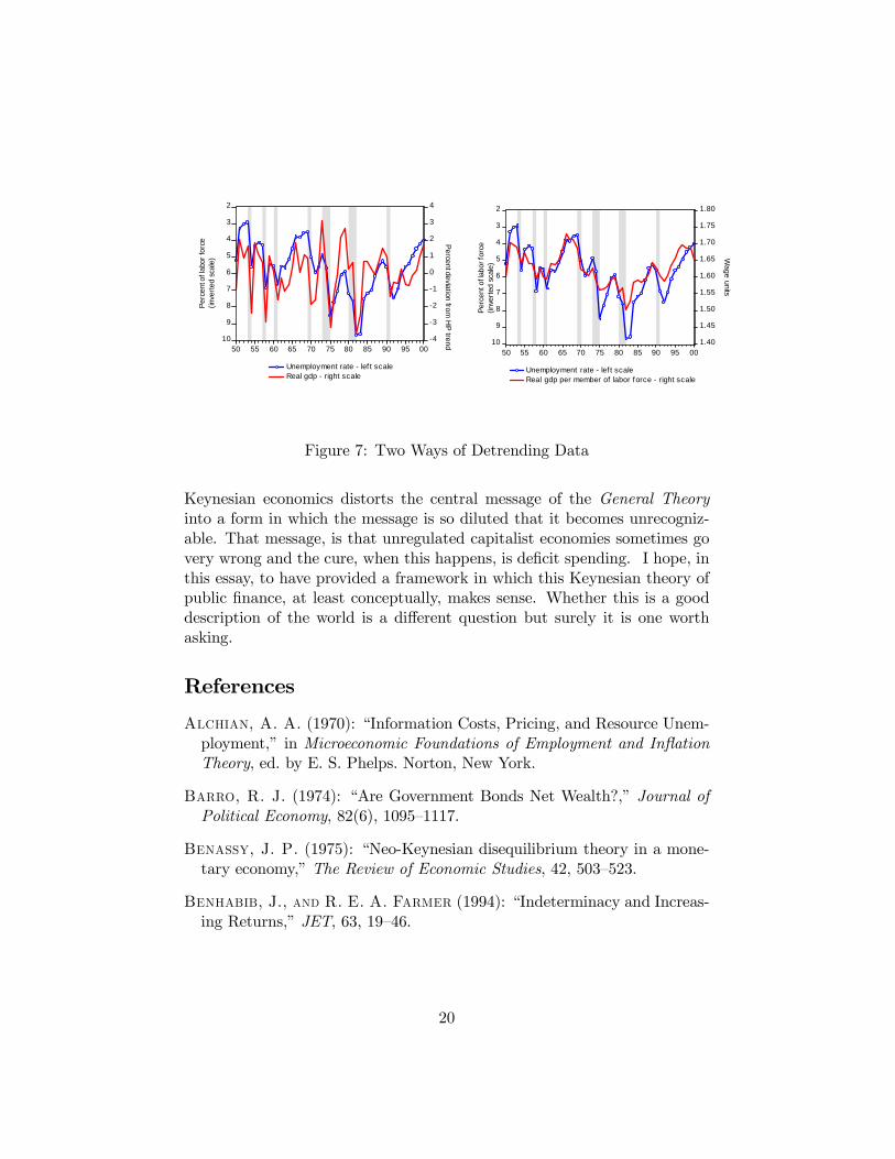
I want to raise one further issue in this essay that relates to the way thatmacroeconomists report data. Since the work of Hodrick and Prescott(1997), macroeconomic data has typically been detrended with a two-sidedfilter. Since the models I am interested in may contain important low fre-quency relationships between series; detrending each individual series bya separate low frequency component is not very sensible since it removesrelevant information from the data that could potentially discriminate be-tween theories. I will be concerned with the question: Is the long-run rateof unemployment is a function of fiscal policy? To answer a question of thiskind I need a way of detrending data that does not remove a different lowfrequency component from each series.

The data reported in this paper was detrended by a method suggestedby Keynes in the General Theory. This involves deflating nominal series by

18

0.995

1.000

1.005

1.010

1.015

1.020

1.025

50 55 60 65 70 75 80 85 90 95 00

Total consumption in wage unitsOptimal consumption

Figure 6: Equilibrium and Optimal Consumption Compared

a measure of the nominal wage to arrive at series measured in “wage units”.Figure 6 compares unemployment with gdp detrended using the HP filter(left panel) with this alternative method. Notice that when GDP is mea-sured this way, it moves much more closely with unemployment (measuredon the left axis using an inverse scale).

5 Conclusion

It is a dangerous business to claim to have uncovered the meaning of Keynesand although it has become fashionable recently to assert that the GeneralTheory was a misstep in the history of thought, I do not take that view.I am old enough (just) to have learned Keynesian economics at graduateschool, as well as as an undergraduate, and foolish enough to have believedat least part of what I was taught.

In distilling a complex book like the General Theory into a logically co-herent argument one necessarily makes compromises since the pieces of thejigsaw come from different puzzles. The task is infinitely more complicatedwhen one is required fit them together with modern ideas that adopt thefiction of the representative agent, the aggregate production function, com-plete contingent claims markets and so on. But it is equally distressing whenthe accepted interpretation of the Keynesian heritage in the form of new-

19

2

3

4

5

6

7

8

9

10 -4

-3

-2

-1

0

1

2

3

4

50 55 60 65 70 75 80 85 90 95 00

Unemployment rate - lef t scaleReal gdp - right scale

Per

cent

of l

abor

forc

e(in

vert

ed s

cale

)

Percent deviation from

HP

trend

2

3

4

5

6

7

8

9

10 1.40

1.45

1.50

1.55

1.60

1.65

1.70

1.75

1.80

50 55 60 65 70 75 80 85 90 95 00

Unemployment rate - lef t scaleReal gdp per member of labor force - right scale

Wage units

Per

cent

of l

abor

forc

e(in

vert

ed s

cale

)

Figure 7: Two Ways of Detrending Data

Keynesian economics distorts the central message of the General Theoryinto a form in which the message is so diluted that it becomes unrecogniz-able. That message, is that unregulated capitalist economies sometimes govery wrong and the cure, when this happens, is deficit spending. I hope, inthis essay, to have provided a framework in which this Keynesian theory ofpublic finance, at least conceptually, makes sense. Whether this is a gooddescription of the world is a different question but surely it is one worthasking.

References

Alchian, A. A. (1970): “Information Costs, Pricing, and Resource Unem-ployment,” in Microeconomic Foundations of Employment and InflationTheory, ed. by E. S. Phelps. Norton, New York.

Barro, R. J. (1974): “Are Government Bonds Net Wealth?,” Journal ofPolitical Economy, 82(6), 1095—1117.

Benassy, J. P. (1975): “Neo-Keynesian disequilibrium theory in a mone-tary economy,” The Review of Economic Studies, 42, 503—523.

Benhabib, J., and R. E. A. Farmer (1994): “Indeterminacy and Increas-ing Returns,” JET, 63, 19—46.

20

Benhabib, J., R. Rogerson, and R. Wright. (1991): “Homework inMacroeconomics: Household Production and Aggregate Fluctuations,”Journal of Political Economy, 99, 1166—87.

Dreze, J. H. (1975): “Existence of an exchange economy with price rigidi-ties,” Interntaional Economic Review, 16, 310—320.

Epstein, L. G., and J. A. Hynes (1983): “The Rate of Time Preferenceand Dynamic Economic Analysis,” Journal of Political Economy, 91, 611—635.

Farmer, R. E. A., and J. T. Guo (1994): “Real Business Cycles and theAnimal Spirits Hypothesis,” JET, 63, 42—73.

Farmer, R. E. A., and A. Lahiri (2005): “Recursive Preferences andBalanced Growth,” Journal of Economic Theory, 125, 61—77.

Friedman, M. (1968): “The Role of Monetary Policy,” American EconomicReview, 58(March), 1—17.

Hodrick, R. J., and E. C. Prescott. (1997): “Post-war U.S. businesscycles: A descriptive empirical investigation.,” Journal of Money Creditand Banking, 29, 1—16.

Keynes, J. M. (1936): The General Theory of Employment, Interest andMoney. MacMillan and Co.

Leeper, E. M. (1991): “Equilibria Under ‘Active’ and ‘Passive’ Monetaryand Fiscal Policies,” Journal of Monetary Economics, 27(1), 129—147.

Leijonhufvud, A. (1966): On Keynesian Economics and the Economicsof Keynes. Oxford University Press.

Lucas, Jr., R. E. (1987): Models of Business Cycles. Basil Blackwell,Oxford, UK.

Lucas, R. E. J., and N. L. Stokey (1984): “Optimal Growth with ManyConsumers,” Journal of Economic Theory, 32, 139—171.

Malinvaud, E. (1977): The theory of unemployment reconsidered. BasilBlackwell, Oxford.

Moen, E. (1997): “Competitive Search Equilibrium,” Journal of PoliticalEconomy, 105(2), 385—411.

21

Phelps, E. S. (1968): “Money wage dynamics and labor market equilib-rium,” Journal of Political Economy, 76, 678—711.

Phelps, E. S. (1970): “The New Microeconomics in Inflation and Em-ployment Theory,” in Microeconomic Foundations of Employment andInflation Theory, ed. by E. S. Phelps. Norton, New York.

Uzawa, H. (1968): “Time Preference, the Consumption Function, and Op-timal Asset Holdings,” in Value, Capital and Growth: papers in Honorof Sir John Hicks, ed. by J. N. Wolfe. Edinburgh University Press, Edin-burgh.

22