Oil spill response planning with consideration of physicochemical evolution of the oil slick: A multiobjective optimization approach

Zhixia Zhong1 and Fengqi You2*

11512 Lakeview Drive, Darien, IL 60561 2Argonne National Laboratory, 9700 S. Cass Avenue, Argonne, IL 60439

August 2010

To be submitted to Computers & Chemical Engineering

Abstract This paper addresses the optimal planning of oil spill response operations under the

constraints of economic and responsive criteria, with consideration of oil transport and

weathering process. The economic criterion is measured in terms of total cost, while the

responsiveness is measured by the time span of the entire response operations. A bi-

criterion, multiperiod mixed-integer linear programming (MILP) model is developed that

minimizes the total cost and the response time span and simultaneously predicts the

optimal time trajectories of the oil slick’s volume and area, transportation profile, usage

levels of response resources, oil spill cleanup schedule, and coastal protection plan. The

MILP model also integrates with the prediction of an oil transport and weathering model

that takes into account oil physiochemical properties, spilled amount, hydrodynamics,

and weather and sea conditions. The multi-objective optimization model is solved with

the ε-constraint method and produces a Pareto-optimal curve that reveals how the optimal

total cost, oil spill cleanup operations, and coastal protection plans change under different

specifications of the response time span. We present two case studies for oil spill

incidents in the Gulf of Mexico area and the New England region to illustrate the

application of the proposed approach.

Key words: planning, oil spill response, MILP, multi-objective optimization, ODE

* To whom all correspondence should be addressed. Tel: (630) 252-4669. Fax: (630)-252-5986. E-mail: youf@mcs.anl.gov. Mailing address: Argonne National Laboratory, 9700 S. Cass Avenue, Building 240, Argonne, IL 60439

-1-

1. Introduction The recent Deepwater Horizon oil spill in the Gulf of Mexico has become the focus

of public attention due to its significant ecological, economic and social impacts (see

http://www.deepwaterhorizonresponse.com/ and http://www.restorethegulf.gov/). This

incident, coupled with previous catastrophic oil spills (e.g., 1989 Exxon Valdez oil spill),

has demonstrated the importance of developing responsive and effective oil spill response

planning strategies for the government and for the oil exploration and production

industries (NOAA, 1992). Under the Oil Pollution Act of 1990 (OPA 90) the party

responsible for the spill is obligated to conduct response operations that satisfy all

requirements set by the Coast Guard. Oil spill response usually occurs within a complex

environment that requires timely decisions to balance the response cost and

responsiveness and to address such issues as weathering and movement of the oil slick,

selection of response/cleanup methods, coordination of coastal protection activities,

availability of cleanup facilities, legal constraints, and performance degradation with bad

weather. This is usually a nontrivial task for decision makers (incident commanders), who

must coordinate considerable resources and must plan many operations. For instance, in

the response to the Deepwater Horizon oil spill, over 39,000 personnel, 5,000 vessels,

and 110 aircraft were involved, over 700 kilometer boom has been deployed, 275

controlled burns have been carried out, approximately 27 million gallons of oily liquid

has been recovered by skimmers, and more than 1.5 million gallons of chemical

dispersant (Corexit) have been used as of July 1, 2010. Therefore, development of

optimal planning strategies for oil spill response operations is critical, in order to balance

the total cost and responsiveness.

Planning problems have been studied extensively by the process systems engineering

community in the recent years. General reviews on this topic are given by Reklaitis

(2000), by Kallrath (2002), and by Verderame et al (2010). Although most of the existing

planning models have only one objective function to maximize the economic

performance, some use a multi-objective optimization scheme to account for such

additional objectives as environmental damage (Bojarski et al., 2009; Guillen-Gosalbez

& Grossmann, 2009; Duque et al., 2010), service level (You et al., 2010), financial risk

(Rodera et al., 2002; You et al., 2009), responsiveness (You & Grossmann, 2008, 2009 &

-2-

2010), and flexibility (Ierapetritou & Pistikopoulos, 1994). The methodology of process

planning has been used in a wide spectrum of applications in process industries, including

chemical production (Verderame & Floudas, 2009), refinery operations (Neiro & Pinto,

2005) new production development (Maravelias & Grossmann, 2001), pharmaceutical

manufacturing (Gatica et al., 2003), and water network (Laird et al., 2006). None,

however, has been extended to deal with the decision-making problems in oil spill

response.

On the other hand, most modeling literature on oil spill is focused on the simulation

of oil transport and weathering process (Brebbia, 2001; Reed et al., 1999), and few have

addressed the response planning problem. A review of the planning models for oil spill

response is given by Iakovou et al (1994). For example, Psaraftis and Ziogas (1985)

developed an integer programming model for optimal dispatching of oil spill cleanup

equipments with the objective to minimize the total response costs. Wilhelm and

Srinivasa (1997) developed an integer programming model for prescribing the tactical

response of oil spill cleanup operations with the objective of minimizing the total

response time of equipments. Limited literature exists that addresses the integration of oil

properties, the weathering model, and the planning model (Ornitz & Champ, 2003). In a

recent work by Gkonis et al,(2007) the authors presented a mixed-integer linear

programming model that considers the oil weathering process, an important factor for

decision making in response operations. None these planning models, however, has taken

into account coastal protection planning, which is usually required for massive oil spills.

Moreover, only a single objective is used in the existing literature; and the time span of

the entire response operations, which is the measure of the responsiveness, has not been

considered by the existing optimization models.

The objective of this paper is to develop an optimization approach to tactical oil spill

response planning under the constraints of economic and responsiveness criteria. The

economic criterion is measured by the total response cost, and responsiveness is

measured by the time span of the entire response operations. We consider both oil spill

cleanup and coastal protection operations in this work. A bi-criterion, multiperiod mixed-

integer linear programming (MILP) model is developed and coupled with the predictions

from an oil transport and weathering model that takes into account the time-dependent oil

-3-

properties, spilled amount, hydrodynamics, weather, and sea conditions. The planning

model simultaneously predicts the optimal time trajectories of the oil slick’s volume and

area, transportation and usage levels of response resources, oil spill cleanup schedule, and

coastal protection plan. The multi-objective optimization model is solved with the ε-

constraint method and produces a Pareto-optimal curve that reveals how the optimal total

cost, oil spill cleanup operations, and coastal protection plans change under different

specifications of the response time span. The application of the proposed optimization

approach is illustrated through two examples based on the incidents of Deepwater

Horizon oil spill and the Argo Merchant oil spill.

This paper includes several novel features. First, we use a multi-objective

optimization approach to consider both economic and responsiveness objectives in the oil

spill response planning. To the best of our knowledge, the responsiveness objective

measured by the time span of the entire response operations has not been considered in

the existing literature. Besides, the multi-objective optimization scheme for the tradeoff

between these two important attributes of oil spill response operations, economics and

responsiveness, was not addressed by any previous work. Second, the proposed model

considers not only the mechanical cleanup method but also in situ burning and chemical

dispersant methods, which were not taken into account in previous work. Third, coastal

protection planning is integrated with oil weathering process and cleanup planning

decisions in the proposed model; this issue has not been reported before as far as we

know.

The rest of this paper is organized as follows. Section 2 presents background on oil

transport, the weathering process, and response operations. We provide a general problem

statement in Section 3. The detailed model formulation of the oil spill response planning

model is given in Section 4, which is followed by the solution approach introduced in

Section 5. In Section 6, we present computational results for two case studies. Section 7

summarizes our conclusions and briefly discusses future work. The formulation of an oil

transport and weathering model is given in the appendix.

2. Background Oil spill response planning requires an effective integration of the physical and

-4-

chemical properties, transport, and weathering of spilled oil; weather and sea conditions;

planning of coastal protection operations; selection of cleanup methods; and scheduling

of cleanup facilities. The spilled oils are normally mixtures of hydrocarbon compounds

whose chemical and physical properties vary among oil types. When an oil spill occurs,

the nature of the oil undergoes a series of changes in chemical and physical properties

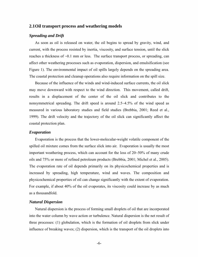
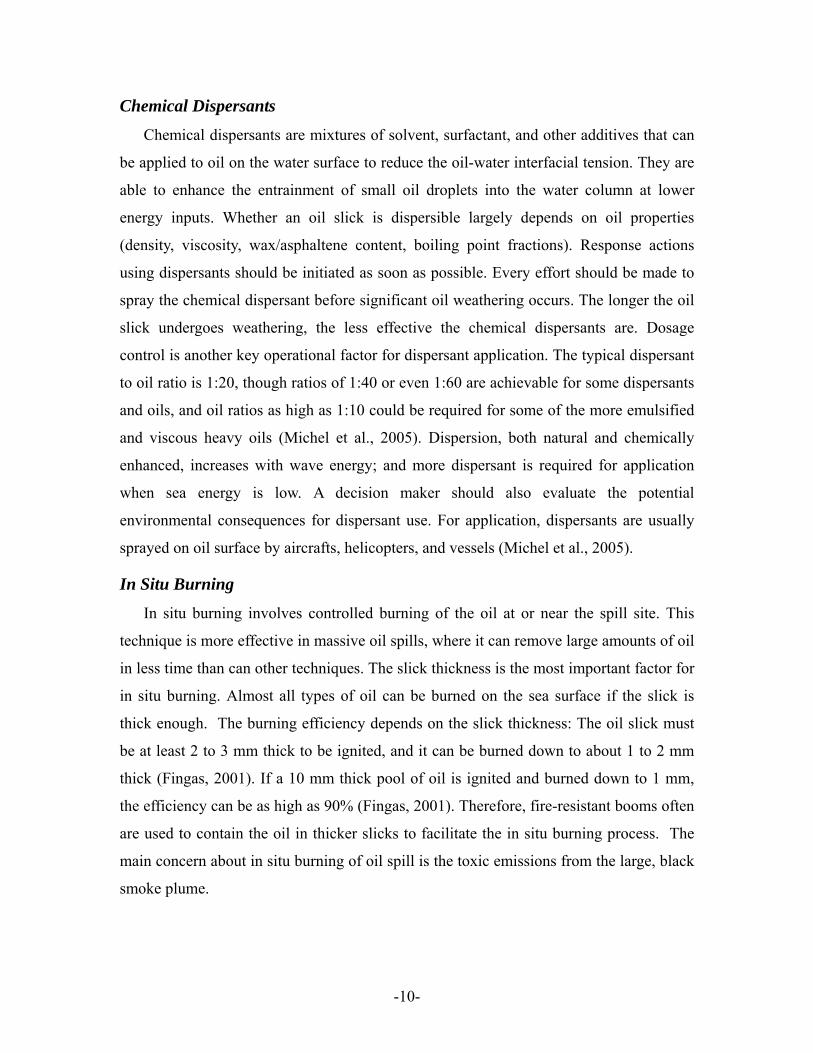
over time that, in combination, are termed “weathering.” In this section, we briefly

review the oil weathering processes including short-term processes such as spreading,

drift, evaporation, emulsification, dispersion, and dissolution and long-term processes

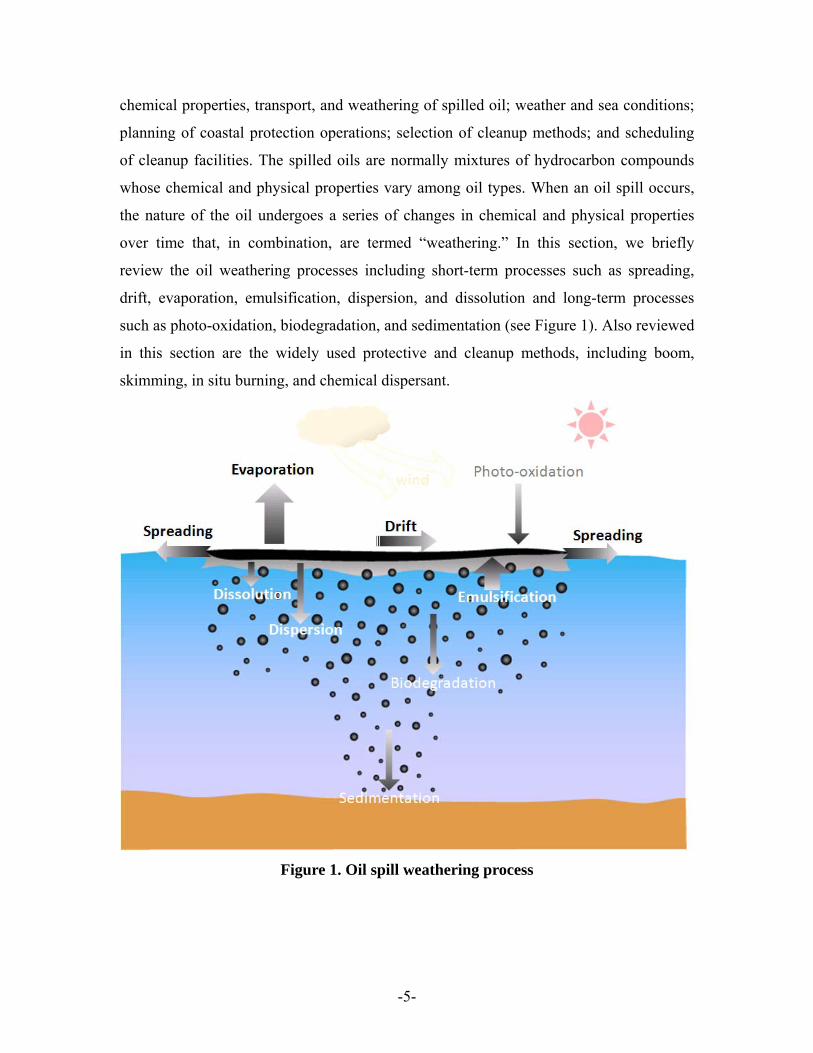
such as photo-oxidation, biodegradation, and sedimentation (see Figure 1). Also reviewed

in this section are the widely used protective and cleanup methods, including boom,

skimming, in situ burning, and chemical dispersant.

Figure 1. Oil spill weathering process

-5-

2.1 Oil transport process and weathering models

Spreading and Drift

As soon as oil is released on water, the oil begins to spread by gravity, wind, and

current, with the process resisted by inertia, viscosity, and surface tension, until the slick

reaches a thickness of ~0.1 mm or less. The surface transport process, or spreading, can

affect other weathering processes such as evaporation, dispersion, and emulsification (see

Figure 1). The environmental impact of oil spills largely depends on the spreading area.

The coastal protection and cleanup operations also require information on the spill size.

Because of the influence of the winds and wind-induced surface currents, the oil slick

may move downward with respect to the wind direction. This movement, called drift,

results in a displacement of the center of the oil slick and contributes to the

nonsymmetrical spreading. The drift speed is around 2.5~4.5% of the wind speed as

measured in various laboratory studies and field studies (Brebbia, 2001; Reed et al.,

1999). The drift velocity and the trajectory of the oil slick can significantly affect the

coastal protection plan.

Evaporation

Evaporation is the process that the lower-molecular-weight volatile component of the

spilled oil mixture comes from the surface slick into air. Evaporation is usually the most

important weathering process, which can account for the loss of 20~50% of many crude

oils and 75% or more of refined petroleum products (Brebbia, 2001; Michel et al., 2005).

The evaporation rate of oil depends primarily on its physicochemical properties and is

increased by spreading, high temperature, wind and waves. The composition and

physicochemical properties of oil can change significantly with the extent of evaporation.

For example, if about 40% of the oil evaporates, its viscosity could increase by as much

as a thousandfold.

Natural Dispersion

Natural dispersion is the process of forming small droplets of oil that are incorporated

into the water column by wave action or turbulence. Natural dispersion is the net result of

three processes: (1) globulation, which is the formation of oil droplets from slick under

influence of breaking waves; (2) dispersion, which is the transport of the oil droplets into

-6-

the water column as a net result of the kinetic energy of oil droplets supplied by the

breaking waves and the rising forces; and (3) coalescence of the oil droplets with the

slick (CONCAWE, 1983).

Natural dispersion reduces the volume of slick on the sea surface and the evaporative

loss, but it does not lead to changes in the physicochemical properties of the spilled oil in

the way those other processes (e.g., evaporation) do. If droplets are small enough, natural

turbulence will prevent the oil from resurfacing. The rate of natural dispersion is an

important factor for the life of an oil slick on the sea surface. In practice, natural

dispersion can be significant, accounting for a major part of the removal of oil from the

sea surface. The effect of natural dispersion depends on both the oil properties and the

amount of sea energy.

Emulsification

Emulsification is the process whereby water droplets are entrained into the oil layer

and remain in the oil slick in unstable, semi-stable, and stable forms. Emulsification can

change the physicochemical properties of oils dramatically, especially for viscosity. The

emulsified oil can contain up to ~70% water. More significant, the oil viscosity can

increase as much as a thousandfold, making the emulsion very difficult to clean up. Once

stable emulsion forms, other weathering processes are also affected. The evaporation and

biodegradation slow, and the spreading and dissolution almost cease. Whether the

emulsification occurs depends on the oil properties. Light, refined oils generally will not

emulsify since they do not contain the right hydrocarbon components to stabilize the

water droplets. Crude oil will emulsify when the wax and asphaltene content reach 5%.

Some oils will emulsify only after they have been weathering to an extent. Emulsions are

characterized as stable, meso-stable, and unstable when the maximum amount of

contained water is 60–80%, 40–60%, and 30–40%, respectively (Sebastiao & Sores,

1995). Most emulsification models are derived from the formulation proposed by Mackay

& McAuliffe (1988) to predict the water content, viscosity, and density of the emulsion.

Other Weathering Processes

Other weathering processes include dissolution, photo-oxidation, sedimentation, and

biodegradation. Dissolution occurs immediately after the oil spill, and the amount is

-7-

usually much less than that from evaporation. Photo-oxidation can change the

composition of spilled oil, but it is not considered to be an important process because it

affects less than 1% of the oil in the slick. Sedimentation is the adhesion of oil to solid

particles in water; it has little effect in removing oil in open-sea conditions.

Biodegradation is a slow, long-term process, and there is no general mathematical model

to describe the biodegradation rate of crude oil in a marine environment. Because of

these limitations, these processes are generally not considered in the mass balance or

physicochemical property changes of the oil weathering model.

2.2 Cleanup and coastal protection methods

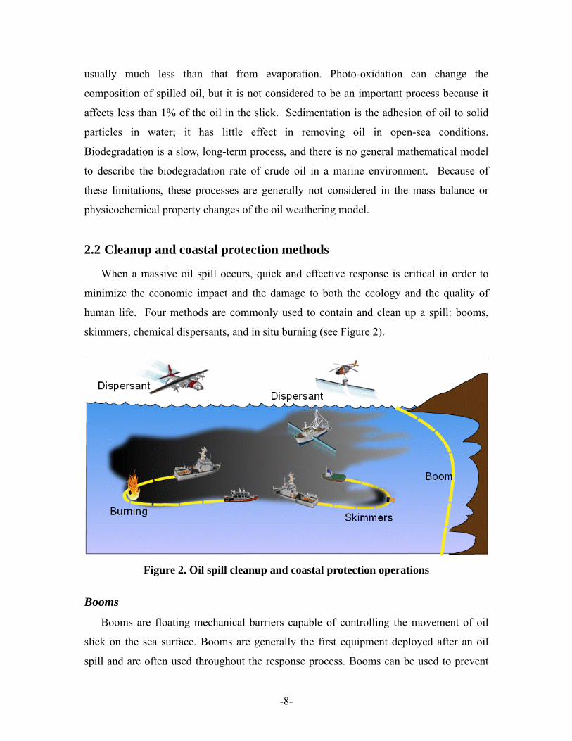
When a massive oil spill occurs, quick and effective response is critical in order to

minimize the economic impact and the damage to both the ecology and the quality of

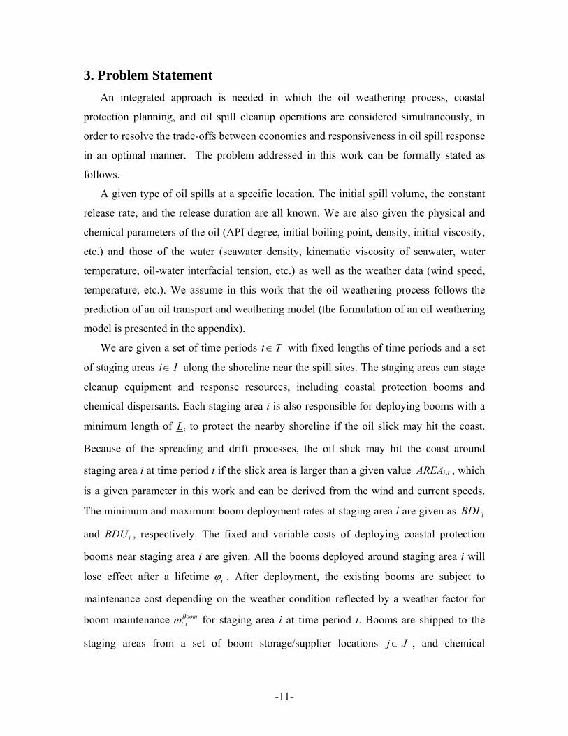
human life. Four methods are commonly used to contain and clean up a spill: booms,

skimmers, chemical dispersants, and in situ burning (see Figure 2).

Figure 2. Oil spill cleanup and coastal protection operations

Booms

Booms are floating mechanical barriers capable of controlling the movement of oil

slick on the sea surface. Booms are generally the first equipment deployed after an oil

spill and are often used throughout the response process. Booms can be used to prevent

-8-

oil from spreading, to protect shorelines, to divert oil to areas where it can be treated or

recovered, or to concentrate oil so that skimmers can be used or in situ burning can be

applied. All booms need to be placed and maintained in a coordinated strategy with other

response approaches to ensure their effectiveness. Booms must be deployed before the

arrival of oil for effective coastal protection. The boom’s performance and ability to

contain oil are affected by currents and winds. When the current speed exceeds a critical

velocity or booms are damaged, boom failure or loss of oil can result. Thus, boom

maintenance, including periodic checks, repairs, and resets, is necessary for effective

coastal protection. There are several types of booms, including conventional hard booms,

fire booms, and sorbent booms. Conventional booms are subject to damages over a

certain time period. Fire booms can withstand high temperatures and are usually used to

contain or concentrate oils for in situ burning. Sorbent booms are made of porous sorbent

material; they are used both to contain and to recover oil, specifically by removing traces

of oil or sheen when oil slick is relatively thin. They are also used as a backup for other

booms and are widely used to improve the performance of conventional hard booms by

absorbing oil Sorbent booms require continuous maintenance, including reposition and

turning to expose a clean surface, and must be replaced when they are saturated by either

oil or water.

Skimmers

Skimmers are mechanical devices designed to recover oil or oil-water mixtures from

the water surface. The effectiveness of a skimmer is rated according to the amount of oil

it recovers. Most skimmers function best when the oil slick is relatively thick; hence,

they are usually placed in front of the boom or where the oil is most concentrated, in

order to recover as much oil as possible. Skimmers can be classified according to their

basic operating principles as oleophilic surface skimmers, weir skimmers,

suction/vacuum skimmers, elevating skimmers, submersion skimmers, and

vortex/centrifugal skimmers. A skimmer’s performance is affected by a number of

factors including the thickness of the oil, the extent of weathering and emulsification of

the oil, the presence of debris, and weather conditions.

-9-

Chemical Dispersants

Chemical dispersants are mixtures of solvent, surfactant, and other additives that can

be applied to oil on the water surface to reduce the oil-water interfacial tension. They are

able to enhance the entrainment of small oil droplets into the water column at lower

energy inputs. Whether an oil slick is dispersible largely depends on oil properties

(density, viscosity, wax/asphaltene content, boiling point fractions). Response actions

using dispersants should be initiated as soon as possible. Every effort should be made to

spray the chemical dispersant before significant oil weathering occurs. The longer the oil

slick undergoes weathering, the less effective the chemical dispersants are. Dosage

control is another key operational factor for dispersant application. The typical dispersant

to oil ratio is 1:20, though ratios of 1:40 or even 1:60 are achievable for some dispersants

and oils, and oil ratios as high as 1:10 could be required for some of the more emulsified

and viscous heavy oils (Michel et al., 2005). Dispersion, both natural and chemically

enhanced, increases with wave energy; and more dispersant is required for application

when sea energy is low. A decision maker should also evaluate the potential

environmental consequences for dispersant use. For application, dispersants are usually

sprayed on oil surface by aircrafts, helicopters, and vessels (Michel et al., 2005).

In Situ Burning

In situ burning involves controlled burning of the oil at or near the spill site. This

technique is more effective in massive oil spills, where it can remove large amounts of oil

in less time than can other techniques. The slick thickness is the most important factor for

in situ burning. Almost all types of oil can be burned on the sea surface if the slick is

thick enough. The burning efficiency depends on the slick thickness: The oil slick must

be at least 2 to 3 mm thick to be ignited, and it can be burned down to about 1 to 2 mm

thick (Fingas, 2001). If a 10 mm thick pool of oil is ignited and burned down to 1 mm,

the efficiency can be as high as 90% (Fingas, 2001). Therefore, fire-resistant booms often

are used to contain the oil in thicker slicks to facilitate the in situ burning process. The

main concern about in situ burning of oil spill is the toxic emissions from the large, black

smoke plume.

-10-

3. Problem Statement An integrated approach is needed in which the oil weathering process, coastal

protection planning, and oil spill cleanup operations are considered simultaneously, in

order to resolve the trade-offs between economics and responsiveness in oil spill response

in an optimal manner. The problem addressed in this work can be formally stated as

follows.

A given type of oil spills at a specific location. The initial spill volume, the constant

release rate, and the release duration are all known. We are also given the physical and

chemical parameters of the oil (API degree, initial boiling point, density, initial viscosity,

etc.) and those of the water (seawater density, kinematic viscosity of seawater, water

temperature, oil-water interfacial tension, etc.) as well as the weather data (wind speed,

temperature, etc.). We assume in this work that the oil weathering process follows the

prediction of an oil transport and weathering model (the formulation of an oil weathering

model is presented in the appendix).

We are given a set of time periods t T∈ with fixed lengths of time periods and a set

of staging areas i along the shoreline near the spill sites. The staging areas can stage

cleanup equipment and response resources, including coastal protection booms and

chemical dispersants. Each staging area i is also responsible for deploying booms with a

minimum length of

I∈

iL to protect the nearby shoreline if the oil slick may hit the coast.

Because of the spreading and drift processes, the oil slick may hit the coast around

staging area i at time period t if the slick area is larger than a given value ,i tAREA , which

is a given parameter in this work and can be derived from the wind and current speeds.

The minimum and maximum boom deployment rates at staging area i are given as iBDL

and iBDU , respectively. The fixed and variable costs of deploying coastal protection

booms near staging area i are given. All the booms deployed around staging area i will

lose effect after a lifetime iϕ . After deployment, the existing booms are subject to

maintenance cost depending on the weather condition reflected by a weather factor for

boom maintenance for staging area i at time period t. Booms are shipped to the

staging areas from a set of boom storage/supplier locations

,Boomi tω

j J∈ , and chemical

-11-

dispersants are similarly shipped from a set of supplier locations k . The

corresponding available amount at the supplier location, transportation time, unit

purchase and shipping costs, transportation capacity, and the inventory holding cost of

booms and chemical dispersants are given.

K∈

The major cleanup methods include mechanical cleanup and recovery (skimming), in

situ burning, and chemical dispersant application. The cleanup facilities for mechanical,

burning, and dispersant application are indexed by m, b, and d, respectively. For instance,

the set of chemical dispersant application types may include C-130 Hercules, helicopters,

and vessels mounted with dispersant spray systems. The maximum number of each type

of cleanup facilities that can be staged to each staging area is given; and the

corresponding total response time to notify, mobilize, dispatch, and deploy the system is

known. The operating capacities of the cleanup systems and the corresponding fixed and

variable costs of operations are given. The weather factor for each cleanup method at

time period t is given. The minimum thickness of the oil slick that each in situ burning

system can handle is known, and the price of the recovered oil through each mechanical

skimming system is given. For chemical dispersant systems, the maximum number of

sorties that can be dispatched at time period t, and the corresponding effectiveness factor

and accuracy factor are given. Note that the effectiveness factor may decrease over time

due to oil weathering. There is a limit on the total amount of chemical dispersants that

can be applied in the entire cleanup operation following federal regulations and

ecological impact concerns. The entire response operation finishes when the volume of

the oil on the sea surface is less than or equal to a predefined cleanup target V .

In order to determine the optimal plan of oil spill response operations, one objective

is to minimize the total time span of the response operations. Another objective is to

minimize the total cost over the entire time span. Since the two conflicting objectives

need to be optimized simultaneously, the corresponding problem yields an infinite set of

trade-off solutions. These solutions are Pareto-optimal in the sense that it is impossible to

improve both objective functions simultaneously. This situation implies that any

solutions for which the total response cost and the response time span can be improved

simultaneously are “inferior” solutions that do not belong to the Pareto-optimal curve.

The aim of this work is to determine the tactical oil spill cleanup and coastal protection

-12-

decisions that define the Pareto optimal curve by minimizing the total cost and the total

response time span.

4. Oil Spill Response-Planning Model In this work we propose an optimization approach for tactical decision making in oil

spill response. The optimization model is coupled with the prediction of physicochemical

evolution of the oil slick from a dynamic oil weathering model. Given the characteristics

of the specific oil spill that define the initial conditions and oil-specific model parameters

(see the Appendix), the oil weathering model is simulated up to the time when natural

weathering process reduces the volume of oil on the sea surface to the cleanup target.

Note that in the natural weathering process, no cleanup or coastal protection actions are

taken. The oil volume, slick area, and water content predicted by the oil weathering

model at each discrete time period are then used as input to the optimization problem.

The formulation of the dynamic oil-weathering model, which is not the focus of this work,

is given in the appendix.

The tactical planning model is formulated as a bi-criterion, multiperiod mixed-integer

linear programming (MILP) problem, which predicts the optimal time trajectories of the

oil slick’s volume and area, transportation and usage levels of response resources, oil spill

cleanup schedule, and coastal protection plan with different specifications of the response

time span. Different from the oil weathering model, where a continuous-time

representation is used, in the planning model we discretize the planning horizon into |T|

time periods with Ht as the length of time period t T∈ . The multiperiod formulation is

widely used in oil spill response-planning problems as it can greatly simplify the

modeling and solution process of the planning models (Gkonis et al., 2007; Psaraftis &

Ziogas, 1985; Srinivasa & Wilhelm, 1997; Wilhelm & Srinivasa, 1997). This

representation is also consistent with the real-world practice that most oil spill cleanup

and shoreline protection decisions are made on a hourly or daily basis (i.e. using one hour

or one day as a time period). Three types of constraints are included in this multiperiod

planning model: oil slick constraints (1)–(5), coastal protection constraints (6)–(20), and

cleanup planning constraints (21)–(33). Equation (34) defines the total response time

span, and equation (35) defines the total cost, both of which are objective functions to be

-13-

optimized. A list of indices, sets, parameters, and variables is given in the Nomenclature

section after the appendix. The detailed model formulation is presented in the following

subsections.

4.1 Oil slick constraints

Based on the multiperiod formulation, we define tδ as the thickness of the oil slick at

the end of time period t. A major assumption of this work is that all the cleanup

operations are local effects that change the slick area but not the average slick thickness;

that is, the thickness remains the same as the prediction by the oil natural-weathering

model. Thus, we have the slick thickness at each time period given by ( ) ( )* *t V t A tδ = ,

where V*(t) and A*(t) are the volume and area of the oil slick, respectively, at time t

predicted by the oil weathering model. With the time trajectory of the slick thickness

fixed, the volume of oil slick should be equal to the product of slick area and slick

thickness in all the time periods:

t tv area tδ= ⋅ , t T∀ ∈ , (1)

where vt is the volume of oil slick and areat is the slick area. Both depend on the cleanup

operations and are variables to be optimized.

We further define tθ as the percentage of oil removed from the slick at time period t

by natural weathering (evaporation and dispersion). The value of this parameter can also

be derived from the solution of dynamic oil-weathering model by using the following

equation: * * *( 1t ) ( ) ( 1)t tV t V t VI H V tθ ⎡ ⎤= − − + ⋅ −⎣ ⎦ , where the term VIt Ht accounts for

the volume of oil newly released to the sea surface in time period t. This parameter is

introduced in order to take into account the effects of evaporation and natural dispersion

in the oil spill response-planning model. To some extent, the use of this parameter is

similar to piecewise linear approximation of the time trajectory of the oil volume. Volume

balance of the oil slick shows that the volume of the oil slick in the previous time period

plus the newly released volume of oil to the sea surface through the current time period

should be equal to the summation of the oil volume at the end of the time period and the

oil volume removed from the slick by natural weathering and cleanup operations. Thus,

-14-

we can model the volume balance with the following equations:

1 1 1 1 1 10 0 1M B

t t t t t t tV VI H v V u u uθ= = = = = =+ ⋅ = + ⋅ + + + D= , (2)

1 1M B D

t t t t t t t tv VI H v v u u uθ− −+ ⋅ = + ⋅ + + + t 2t∀ ≥ , (3)

where Mtu , , and B

tu Dtu are the volumes of oil removed from the sea surface by using

mechanical systems (skimmers), in situ burning, and chemical dispersants, respectively.

To model the time span of the oil spill response operations, we introduce a 0-1

variable tf . If the volume of the oil slick is greater than the cleanup target, then tf equals

1; otherwise, it equals zero. Thus, we have the following constraint:

t tv V U f≤ + ⋅ t T∀ ∈ , (4)

where V is the cleanup target and U is a sufficiently large number for the upper bound of

the volume.

If the oil spillage has not yet stopped at time period t, the cleanup target is not

achieved in that time period regardless of the volume of oil remaining on the sea surface:

''

T

t tt t

VI U f=

≤ ⋅∑ t T∀ ∈ . (5)

4.2 Coastal protection constraints

Because of the spreading and drift processes, the oil slick may hit the coast and lead

to significant environmental damage. Booms can be deployed along the coast to protect

sensitive shorelines, but boom protection can be effective if and only if sufficient lengths

of booms are deployed in the corresponding shorelines. In order to protect the coast,

either the slick area must be controlled through effective cleanup operations so that it will

not hit the shore, or coastal protection booms must be fully deployed around those

staging areas that might be hit by the oil slick ( =1). However, this constraint can be

relaxed after the cleanup target is achieved (

,i tz

tf =0); in other words, there is no need to

protect the coasts after the volume of oil is reduced to the cleanup target. The following

inequality models this relationship:

( ), , 1i tt i tarea AREA U z U f≤ + ⋅ + ⋅ − t ,i I t T∀ ∈ ∈ , (6)

-15-

where areat is the area of the oil slick at the end of time period t, ,i tAREA is the area of

the oil slick that will hit the shore around staging area i at time period t, zit is a binary

variable that equals 1 if sufficient booms have been deployed to protect the shoreline

around staging area i at time period t, and U is a sufficiently large number for the upper

bound of oil slick area. ,i tAREA depends primarily on the drifting effect; its value may

decrease over time if wind and current push the oil slick toward the shore, and vice versa.

If sufficient booms have been deployed to protect the shoreline around staging area i

at time period t ( ), the booms must have been deployed at any time before t. This

relationship can be modeled with the following logic proposition:

,i tz

, ,' 1i t i tt tz z

≤ −⇒ ∨ 'd

'd

where is a binary variable that equals 1 if the booms are being deployed around

staging area i to protect the nearby shoreline in time period t. The logic propositions can

be further transformed into inequalities (Raman & Grossmann, 1993):

,i tzd

, ,' 1

i t i tt t

z z≤ −

≤ ∑ ,i I t T∀ ∈ ∈ . (7)

If booms are being deployed at time period t-1 along the shoreline near staging area i

( ), then the boom deployment will continue during time period t ( ) or until

sufficient booms have been deployed to protect the shoreline around this staging area at

the beginning of time period t ( ). In other words, once the boom deployment at a

staging area begins, it will not stop until sufficient booms have been deployed. The

corresponding logic proposition is

, 1i tzd − ,i tzd

,i tz

, 1 , ,i t i t i tzd zd z− ⇒ ∨ ,

which can be transformed into the inequality

, , 1i t i t i tz zd zd−≥ − , ,i I t T∀ ∈ ∈ . (8)

Boom maintenance is required for the shoreline around staging area i at time period t

( ) if and only if the cleanup target has not been achieved (,i tzm tf ) and the coastal

protection booms are being deployed at time period t ( ) or fully deployed to protect

the shoreline around staging area i ( ). This relationship can be modeled with a logic

,i tzd

,i tz

-16-

proposition as follows:

( ), ,i t t i t i tzm f zd z⇔ ∧ ∨ , ,

where is a binary variable that equals 1 if maintenance is required for booms

around staging area i. This logic proposition can be transformed into the following

inequalities.

,i tzm

,i t tzm f≤ ,i I t T∀ ∈ ∈ (9)

, ,i t i t i tzm zd z≤ + , ,i I t T∀ ∈ ∈ (10)

, , 1i t t i tzm f zd≥ + − ,i I t T∀ ∈ ∈ (11)

, , 1i t t i tzm f z≥ + − ,i I t T∀ ∈ ∈ (12)

The shoreline around staging area i is fully protected by the booms at time period t if

and only if the length of boom ( ) is no less than the required length (,i tbl iL ) both at the

beginning and at the end of time period t. Since the length of boom deployed at the

beginning of time period t is the same as the one at the end of time period t-1, we use the

following inequalities to model this constraint:

, , 1i ii t i t i t,L z bl L U z−⋅ ≤ ≤ + ⋅ ,i I t T∀ ∈ ∈ (13)

, ,i ii t i t i t,L z bl L U z⋅ ≤ ≤ + ⋅ ,i I t T∀ ∈ ∈ , (14)

where iL is the length of boom required to protect the shore around staging area i and

is the length of boom deployed along the shore of staging area i at the end of time

period t.

,i tbl

Coastal protection booms deployed at staging area i can be effective for only a certain

lifetime ( iϕ ) after deployment. The length of the boom that fails at time period t is the

same as the length deployed at time period it ϕ− .

, , ii t i tbfail bdep ϕ−= ,i I t T∀ ∈ ∈ (15)

The length of the boom around the shore of staging area i at the end of time period t

( ) is equal to the boom length at the end of the previous time period ( ) plus the

length of the boom deployed at the current time period ( ) minus those that fail at

this time period ( ). Thus, the balance of boom length is given by the following

,i tbl , 1i tbl −

,i tbdep

,i tbfail

-17-

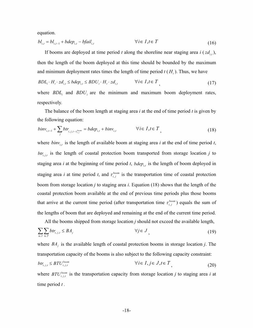
equation. , , 1 ,i t i t i t i tbl bl bdep bfail−= + − , ,i I t T∀ ∈ ∈ (16)

If booms are deployed at time period t along the shoreline near staging area i ( ),

then the length of the boom deployed at this time should be bounded by the maximum

and minimum deployment rates times the length of time period t ( ). Thus, we have

,i tzd

tH

, ,i t i t i t i t iBDL H zd bdep BDU H zd⋅ ⋅ ≤ ≤ ⋅ ⋅ ,t ,i I t T∀ ∈ ∈ , (17)

where iBDL and iBDU are the minimum and maximum boom deployment rates,

respectively.

The balance of the boom length at staging area i at the end of time period t is given by

the following equation:

,, 1 , ,, , boom

i ji t i t i ti j t

j

binv btr bdep binvτ− −

+ = +∑ ,i I t T∀ ∈ ∈ , (18)

where is the length of available boom at staging area i at the end of time period t,

is the length of coastal protection boom transported from storage location j to

staging area i at the beginning of time period t, is the length of boom deployed in

staging area i at time period t, and is the transportation time of coastal protection

boom from storage location j to staging area i. Equation

,i tbinv

, ,i j tbtr

,i tbdep

,boomi jτ

(18) shows that the length of the

coastal protection boom available at the end of previous time periods plus those booms

that arrive at the current time period (after transportation time ) equals the sum of

the lengths of boom that are deployed and remaining at the end of the current time period.

,boomi jτ

All the booms shipped from storage location j should not exceed the available length,

, ,i j t ji I t T

btr BA∈ ∈

≤∑∑ j J∀ ∈ , (19)

where is the available length of coastal protection booms in storage location j. The

transportation capacity of the booms is also subject to the following capacity constraint:

jBA

, , , ,boom

i j t i j tbtr BTU≤ , ,i I j J t T∀ ∈ ∈ ∈ , (20)

where is the transportation capacity from storage location j to staging area i at

time period t .

, ,boomi j tBTU

-18-

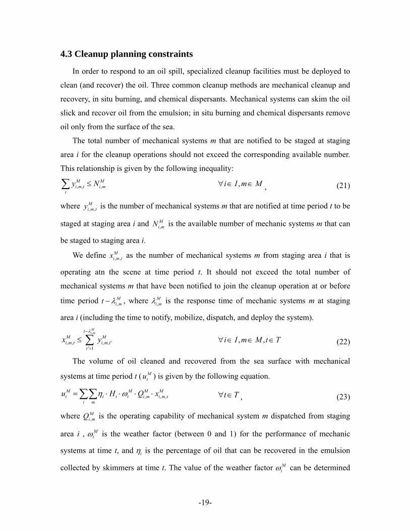
4.3 Cleanup planning constraints

In order to respond to an oil spill, specialized cleanup facilities must be deployed to

clean (and recover) the oil. Three common cleanup methods are mechanical cleanup and

recovery, in situ burning, and chemical dispersants. Mechanical systems can skim the oil

slick and recover oil from the emulsion; in situ burning and chemical dispersants remove

oil only from the surface of the sea.

The total number of mechanical systems m that are notified to be staged at staging

area i for the cleanup operations should not exceed the corresponding available number.

This relationship is given by the following inequality:

, , ,M Mi m t i m

t

y N≤∑ ,i I m M∀ ∈ ∈ , (21)

where , ,Mi m ty is the number of mechanical systems m that are notified at time period t to be

staged at staging area i and ,Mi mN is the available number of mechanic systems m that can

be staged to staging area i.

We define , ,Mi m tx as the number of mechanical systems m from staging area i that is

operating atn the scene at time period t. It should not exceed the total number of

mechanical systems m that have been notified to join the cleanup operation at or before

time period ,Mi mt λ− , where ,

Mi mλ is the response time of mechanic systems m at staging

area i (including the time to notify, mobilize, dispatch, and deploy the system).

,

, , , , '' 1

Mi mt

M Mi m t i m t

tx y

λ−

=

≤ ∑ , ,i I m M t T∀ ∈ ∈ ∈ (22)

The volume of oil cleaned and recovered from the sea surface with mechanical

systems at time period t ( Mtu ) is given by the following equation.

, ,M Mt t t t i m

i m

u H Qη ω= ⋅ ⋅ ⋅ ⋅∑∑ ,M M

i m tx t T∀ ∈ , (23)

where ,Mi mQ is the operating capability of mechanical system m dispatched from staging

area i , Mtω is the weather factor (between 0 and 1) for the performance of mechanic

systems at time t, and tη is the percentage of oil that can be recovered in the emulsion

collected by skimmers at time t. The value of the weather factor Mtω can be determined

-19-

by weather forecasting. For instance, a sunny day with zero wind speed and zero wave

height (i.e., calm sea) has a weather factor close to 1 because skimmers perform best

under such conditions. On the other hand, strong winds and high waves coupled with

heavy rain may lead to a weather factor close to zero. The percentage of oil in the

emulsion ( tη ) can be derived from the fractional water content through the following

equation: , where is the fractional water content at time t based on

the prediction of the oil weathering model.

WY

*1 (t WY t= − )η

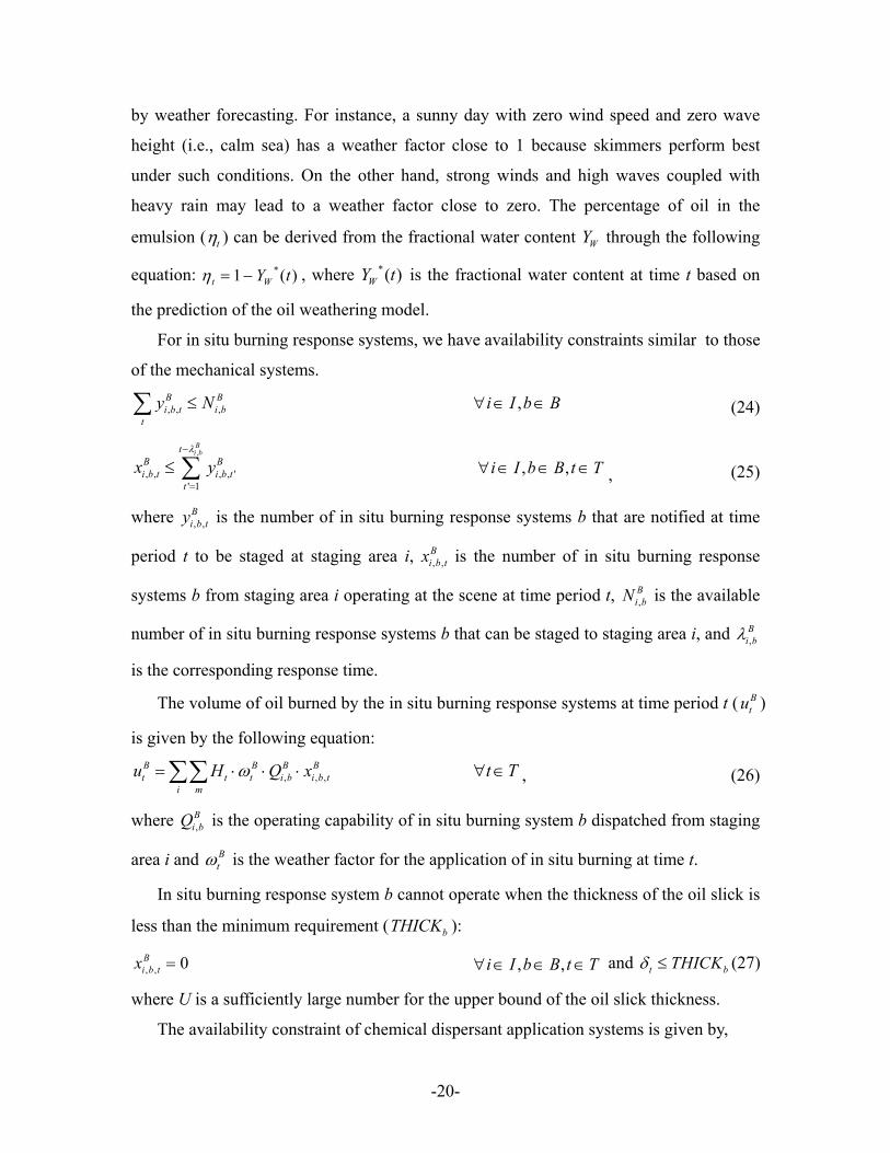
,B B

i b

*( )WY t

For in situ burning response systems, we have availability constraints similar to those

of the mechanical systems.

, ,i b tt

y N≤∑

,i I b B∀ ∈ ∈ (24)

,

'

Bi b

Bt, ,

' 1

tBi b t

t, ,i bx y

λ−

=

≤ ∑ , ,i I b B Tt∀ ∈ ∈ ∈ , (25)

where is the number of in situ burning response systems b that are notified at time

period t to be staged at staging area i,

, ,tByi b

, ,Bi b tx is the number of in situ burning response

systems b from staging area i operating at the scene at time period t, is the available

number of in situ burning response systems b that can be staged to staging area i, and

,Bi bN

,B

i bλ

is the corresponding response time.

The volume of oil burned by the in situ burning response systems at time period t ( )

is given by the following equation:

Btu

, , ,Bi bQ ⋅∑∑B B

ti m

ω= ⋅ ⋅ Bb tt tu H ix

t T∀ ∈ , (26)

where Q is the operating capability of in situ burning system b dispatched from staging

area i and

,Bi b

Btω is the weather factor for the application of in situ burning at time t.

In situ burning response system b cannot operate when the thickness of the oil slick is

less than the minimum requirement ( ): bICKTH

, , 0Bi b tx = , ,i I b B t T∀ ∈ ∈ ∈ and t bTHICKδ ≤ (27)

where U is a sufficiently large number for the upper bound of the oil slick thickness.

The availability constraint of chemical dispersant application systems is given by,

-20-

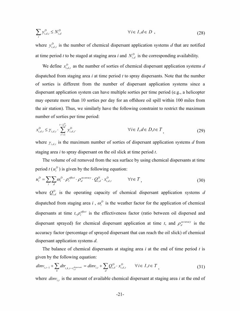
, , ,D Di d t i d

ty N≤∑ ,i I d D∀ ∈ ∈ , (28)

where is the number of chemical dispersant application systems d that are notified

at time period t to be staged at staging area i and

, ,Di d ty

,Di dN is the corresponding availability.

We define , ,Di d tx as the number of sorties of chemical dispersant application systems d

dispatched from staging area i at time period t to spray dispersants. Note that the number

of sorties is different from the number of dispersant application systems since a

dispersant application system can have multiple sorties per time period (e.g., a helicopter

may operate more than 10 sorties per day for an offshore oil spill within 100 miles from

the air station). Thus, we similarly have the following constraint to restrict the maximum

number of sorties per time period:

,

, , , , , , '' 1

Di dt

D Di d t i d t i d t

tx y

λ

γ−

=

≤ ⋅ ∑ , ,i I d D t T∀ ∈ ∈ ∈ , (29)

where , ,i d tγ is the maximum number of sorties of dispersant application systems d from

staging area i to spray dispersant on the oil slick at time period t.

The volume of oil removed from the sea surface by using chemical dispersants at time

period t ( Dtu ) is given by the following equation:

, ,D D effect accuracy D Dt t t d i d i d t

i du ω ρ ρ= ⋅ ⋅ ⋅ ⋅∑∑ ,Q x t T

∀ ∈ , (30)

where ,Di dQ is the operating capacity of chemical dispersant application systems d

dispatched from staging area i , Dtω is the weather factor for the application of chemical

dispersants at time t, is the effectiveness factor (ratio between oil dispersed and

dispersant sprayed) for chemical dispersant application at time t, and is the

accuracy factor (percentage of sprayed dispersant that can reach the oil slick) of chemical

dispersant application systems d.

effecttρ

accuracydρ

The balance of chemical dispersants at staging area i at the end of time period t is

given by the following equation:

,, 1 , , , ,, , dispersant

i k

D Di t i t i d i d ti k t

k ddinv dtr dinv Q x

τ− −+ = +∑ ∑ ⋅ ,i I t T∀ ∈ ∈ , (31)

where is the amount of available chemical dispersant at staging area i at the end of ,i tdinv

-21-

time pe , , ,i k tdtr is the amount of chemical dispersant shipped from supplier location k

to staging area the beginning of time period t, and ,dispersanti kτ is the transportation time

for moving the chemical dispersant from the supplier location k to staging area i . The

term , , ,D Di d i d td

Q x⋅∑ is the total amount of chemical dispersant used by dispersant

applic dispatched from staging area i at time period t. The equation shows

that the amount of chemical dispersant available at the end of previous time periods plus

the amount of dispersant arriving at the current time period (after transportation time

,dispersanti kτ ) equals the sum of the amount of chemical dispersant that is used in the current

iod and the remaining amount at the end of the current time period. Note that we

do not consider the selection of chemical dispersants in this work, because only one type

of dispersant is used in most oil spill responses (Michel et al., 2005).

The chemical dispersants shipped from supplier location k to a

riod t

ll the staging areas

i at

systems ation

pertime

shou

i

ld be less than or equal to the available amount ( ,k tCDS ).

, , ,i k t k tdtr CDS≤∑ k T,K t∀ ∈ ∈

throug

(32)

ical dispersant used

(33)

re included in this model: responsiveness and economics.

(34)

The total amount of chem

Objective functions

t

hout the entire response

ope

.4

Res

Here

ration should not exceed the limit set by the regulator (DLIMIT).

, ,i k ti k t

dtr DLIMIT≤∑∑∑

4

Two objective functions a

ponsiveness is measured by the total time span of the entire response operations,

which can be modeled by the following equation.

min : tTimeSpan f=∑

tf is a binary vari greater thanable that equals 1 if the volume of the oil slick is the

cleanup target or there is oil newly released to the sea surface at time period t. Summation

of all the tf over the planning horizon equals the number of time periods used for the

response operations, because after the spillage stops, the volume of oil slick can only

decrease over time as a result of evaporation and natural dispersion. We should note that

-22-

constraint (5) imposes that tf must be 1 if the oil spillage has not yet stopped at time

period t.

Economics is measured by the total cost, as follows:

min : To , , , , , , , ,

, , , , , , , , , , , ,

M M B B D Di m i m t i b i b t i d i d t

i b t

B D Di m t i m t i b t i b t i d t i d t

i m i b t i b t

talCost y FC y FC y

C x C x C x

CI

= ⋅ + ⋅ +

+ ⋅ + ⋅ + ⋅

+

∑∑∑ ∑∑∑ ∑∑∑

∑∑∑ ∑∑∑ ∑∑∑

, ,

, , , , , ,

, , , ,

rsant boomi i t i i t

i t i t

boom dispersanti j i j t i k i k t

i j i k t

boom boomi t i t i t i t

i t i t

dinv CI binv

btr CT dtr

bdep FCDEP zd

⋅ + ⋅

+ ⋅ + ⋅

+ ⋅ + ⋅

∑∑ ∑∑

∑∑∑ ∑∑∑

∑∑ ∑∑

, , , , ,

boom boomi t i t i t i t

i t i t

Mt

t

CBM bl FCBM zm

u O

ω ⋅ + ⋅

− ⋅

∑∑ ∑∑

∑

,⋅

(35)

where the first three terms are for the fixed cost (including mobilization, equipment

transportation and set-up costs) of staging response systems, the fourth to sixth terms

model properties. We then describe our

m del has the following two properties that can be used to

e ficiency.

can be relaxed as a continuous variable without

changing the optimal solution.

i m t i b t

M M B

t

FC

dispe

t

CT

CDEP

boomi t

C

+ ⋅

o

f

account for operating cost of the cleanup operations, the seventh to tenth terms are the

inventory, purchase and transportation cost of dispersants and coastal protection booms,

the eleventh to fourteenth terms are the fixed and variable costs for boom deployment and

maintenance, and the last term is the credit resulting from the recovery of the spilled oil.

5. Solution Approach

In this section we first discuss two key

optimization procedure. 5.1 Model properties

The proposed MILP

improve its computational

Property 1. The binary variable ,i tzm

-23-

Proof: Because tf , ,i tzd , and ,i tz

.

are all binary variables, constraints (24)–(26) impose

Property 2. The binary variables

that ,i tzm equals eith ero or 1

er z

, ,Mi m ty and can be relaxed as continuous variables

on.

, ,Bi b ty

without changing the optimal soluti

Proof: Variable , ,Mi m ty appears only in constraints (34) and (35) except the objective

function (48). Because M, ,i m tx is an integer variable and parameter ,

Mi mN has an integer

value, the constraints fo riable , ,Mi m tr va y define an integer polyhedron after fixing the

values of other variables (Nemhauser & Wolsey, 1988). Therefore, M, ,i m ty takes only

integer values, and it can be relaxed as a continuous variable. Similarly, we can prove that

, ,Bi b ty has the same property.

,i tzm , , ,Mi m tyBased on these two properties, we can relax integer variables , and

and l.

5.2 olution procedure for multi-objective optimization

timization problem,

one

, ,Bi b ty

improve the computational efficiency of solving the MILP mode

S

In order to obtain the Pareto-optimal curve for the bicriterion op

of the objectives is specified as an inequality with a fixed value for the bound that is

treated as a parameter. Two major approaches can be used to solve the problem in terms

of this parameter. One is simply to solve it for a specified number of points to obtain an

approximation of the Pareto-optimal curve. The other is to solve it as a parametric

programming problem (Dua & Pistikopoulos, 2004), which yields the exact solution for

the Pareto-optimal curve. While the latter approach provides a rigorous solution

approach, the former approach is easier to implement. Moreover, the objective of

response time span is represented by the number of time periods; hence, solving the

problem by minimizing the total cost with all the possible values of time span, which is

finite, will yield the exact solution of the Pareto-optimal curve for the proposed model.

Therefore, we use the ε-constraint method to solve the proposed model. The procedure

-24-

comprises three steps. First, we to minimize the response time span to obtain the shortest

time span TimeSpanS. Second, we minimize the total cost that in turn yields the longest

Pareto-optimal time span TimeSpanL. In this case the objective function is set as

min : TotalCost TimeSpanχ+ ⋅ , (36)

where χ is a very small value (on the order of 0.01). Third, we fix ε to discrete int

be

eger

values tween TimeSpanS and TimeSpanL and add the following constraint to the model

with the objective to minimize TotalCost.

TimeSpan ε≤ (37) In this way w

. Case Studies application of the proposed model, we consider two case studies

base

6.1 ase study 1: oil spill in the Gulf of Mexico

il spill incident in the Gulf of

Mex

e can obtain the exact solution of the Pareto-optimal curve for the proposed

model, together with the optimal solutions for different values of time span.

6To illustrate the

d on the incidents of Deepwater Horizon oil spill in the Gulf of Mexico and Argo

Merchant oil spill in New England. The computational studies were performed on an

IBM T400 laptop with Intel 2.53 GHz CPU and 2 GB RAM. The ordinary differential

equation (ODE) model for the oil transport and weathering processes was coded in

MATLAB and solved with Runge–Kutta fourth/fifth-order method. The MILP model for

oil spill response planning was coded in GAMS 23.4.3 and solved by using CPLEX 12.

The optimality tolerances were all set to 10-9.

C

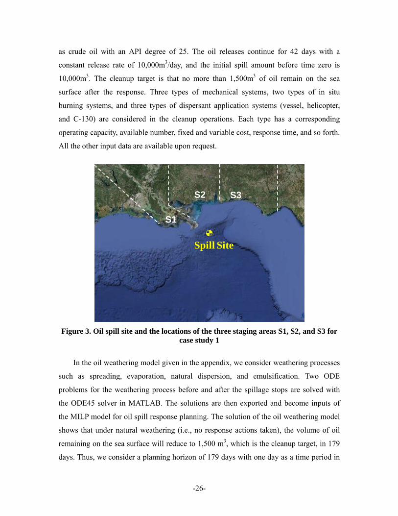
In the first case study, we consider the response to an o

ico area. There are three major staging areas for the response operations: S1, S2, and

S3,. Their locations, along with the spill site, are given in the map in Figure 3. The

minimum distances between the three staging areas and the oil spill site are 60 kilometers,

120 kilometers, and 180 kilometers, respectively. In this case, we assume the oil slick

drifts toward the shore as a result of wind and current directions. The lengths of the

booms required to protect the sensitive coastline near the three staging areas are 200

kilometers, 180 kilometers, and 300 kilometers, respectively. The spilled oil is considered

-25-

as crude oil with an API degree of 25. The oil releases continue for 42 days with a

constant release rate of 10,000m3/day, and the initial spill amount before time zero is

10,000m3. The cleanup target is that no more than 1,500m3 of oil remain on the sea

surface after the response. Three types of mechanical systems, two types of in situ

burning systems, and three types of dispersant application systems (vessel, helicopter,

and C-130) are considered in the cleanup operations. Each type has a corresponding

operating capacity, available number, fixed and variable cost, response time, and so forth.

All the other input data are available upon request.

Spill Site

S1

S2 S3

Figure 3. Oil spill site and the locations of the three staging areas S1, S2, and S3 for

odel given in the appendix, we consider weathering processes

such

case study 1

In the oil weathering m

as spreading, evaporation, natural dispersion, and emulsification. Two ODE

problems for the weathering process before and after the spillage stops are solved with

the ODE45 solver in MATLAB. The solutions are then exported and become inputs of

the MILP model for oil spill response planning. The solution of the oil weathering model

shows that under natural weathering (i.e., no response actions taken), the volume of oil

remaining on the sea surface will reduce to 1,500 m3, which is the cleanup target, in 179

days. Thus, we consider a planning horizon of 179 days with one day as a time period in

-26-

the MILP model. After relaxing integer variables ,i tzm , , ,Mi m ty , and , ,

Bi b ty to reduce the

computational complexity, the MILP-based planni m

variables, 8,543 continuous variables, and 13,884 constraints.

We use the ε–constraint method to obtain the Pareto-optim

ng odel includes 5,499 discrete

al curve and determine the

trade-off between the total response cost and the responsiveness, which is measured by

the response time span. The first step of the ε–constraint method is to determine the

optimal lower and upper bounds of the response time span. The lower bound is obtained

by minimizing (34) subject to constraints (1)–,(33) and the upper bound can be obtained

by minimizing (36) subject to the same constraints. For this problem, we obtain 75 days

as the lower bound of time span and 179 days as the optimal upper bound of time span.

We then solve the problem with fixed values from 75 days to 179 days (105 instances

with increments of one day). The solution process takes a total of 307 CPU-seconds for

all 105 instances.

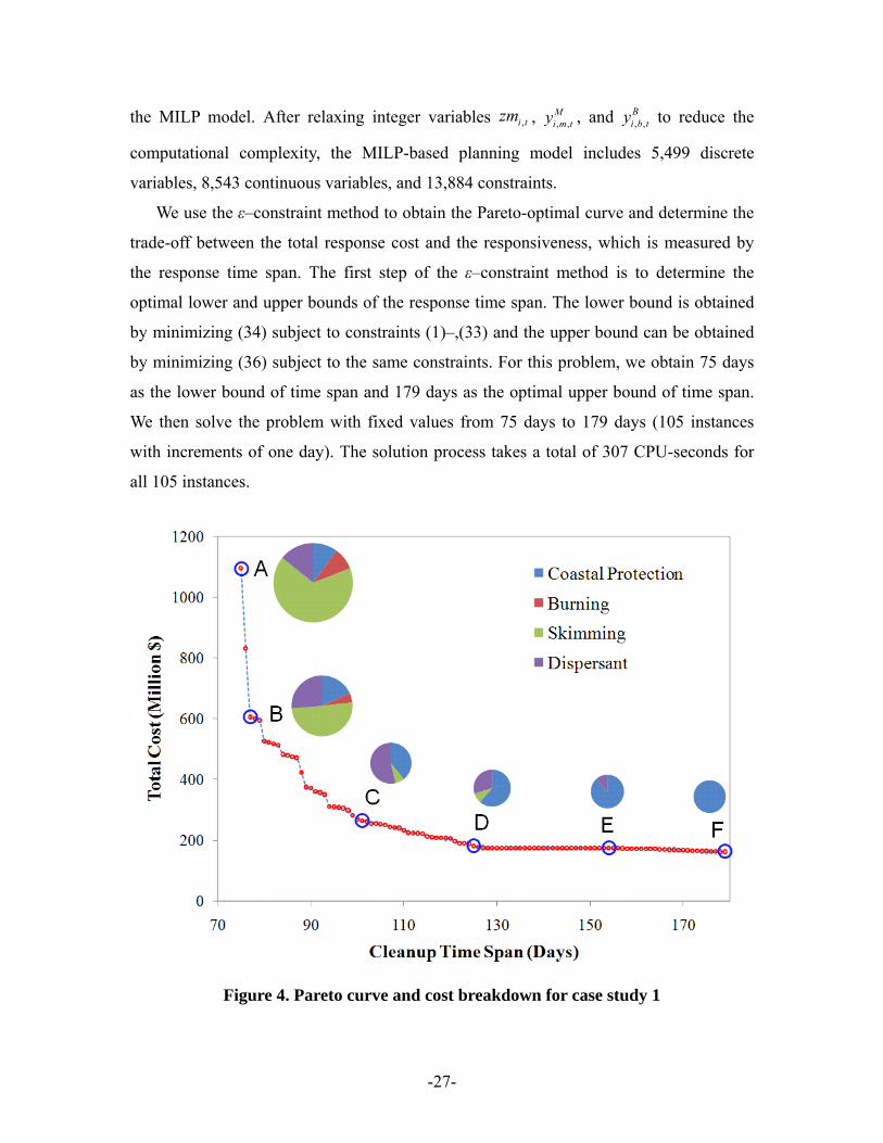
Figure 4. Pareto curve and cost breakdown for case study 1

-27-

The results are given in Figures 4–11. The line in Figure 4 is the Pareto-optimal curve

of t

4 are for the breakdown of the total costs for Points A–F. For

sho

his problem. As can be seen, the total cost ranges from $1,095MM to $162MM, while

the response time span ranges from 75 days to 179 days. Thus, the total cost decreases as

the time span increases. Since the time span is a measure of responsiveness, we can

conclude that the more responsive the response operations is, the more cost it requires. In

particular, when the response time span increases from 75 days (Point A) to 77 days

(Point B), the total cost reduces almost by half. This suggests that 77 days might be a

better choice for the oil spill response based on the trade-off between economics and

responsiveness. Moreover, we can see that when the response time span decreases from

178 days (Point F) to 125 days (Point D), the total cost increases only from $162MM to

$182MM. In other words, a 10% increase of the cost can reduces the response time span

from half a year to four months. Clearly, Point D is a better choice than Point F in the oil

spill response operations.

The pie charts in Figure

rt time spans, most of the cost is for oil spill cleanup (skimming, burning, and

dispersant). Because of the high operational responsiveness in these cases, most of the

shoreline will not be hit by the oil slick, and thus there is relatively low cost for boom

deployment for coastal protection. As the time span increases and the total cost decreases,

more is spent on coastal protection than on oil spill cleanup. The reason is that the least-

cost option for this case study is to deploy booms to protect the sensitive shorelines while

leaving the oil slick on the sea surface until natural weathering reduces the oil volume to

the cleanup target; that is, no cleanup efforts are taken in the least-cost instance.

-28-

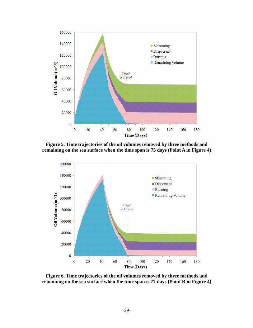
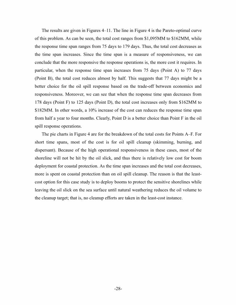
Figure 5. Time trajectories of the oil volumes removed by three methods and

remaining on the sea surface when the time span is 75 days (Point A in Figure 4)

Figure 6. Time trajectories of the oil volumes removed by three methods and

remaining on the sea surface when the time span is 77 days (Point B in Figure 4)

-29-

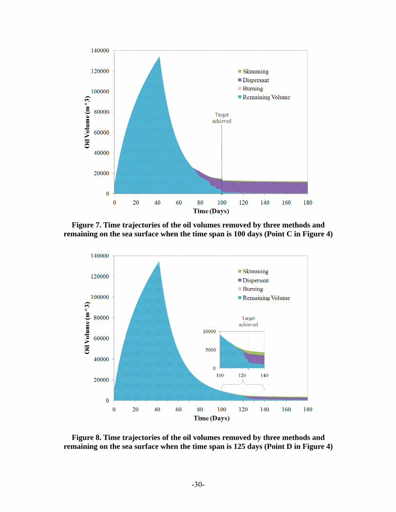
Figure 7. Time trajectories of the oil volumes removed by three methods and

remaining on the sea surface when the time span is 100 days (Point C in Figure 4)

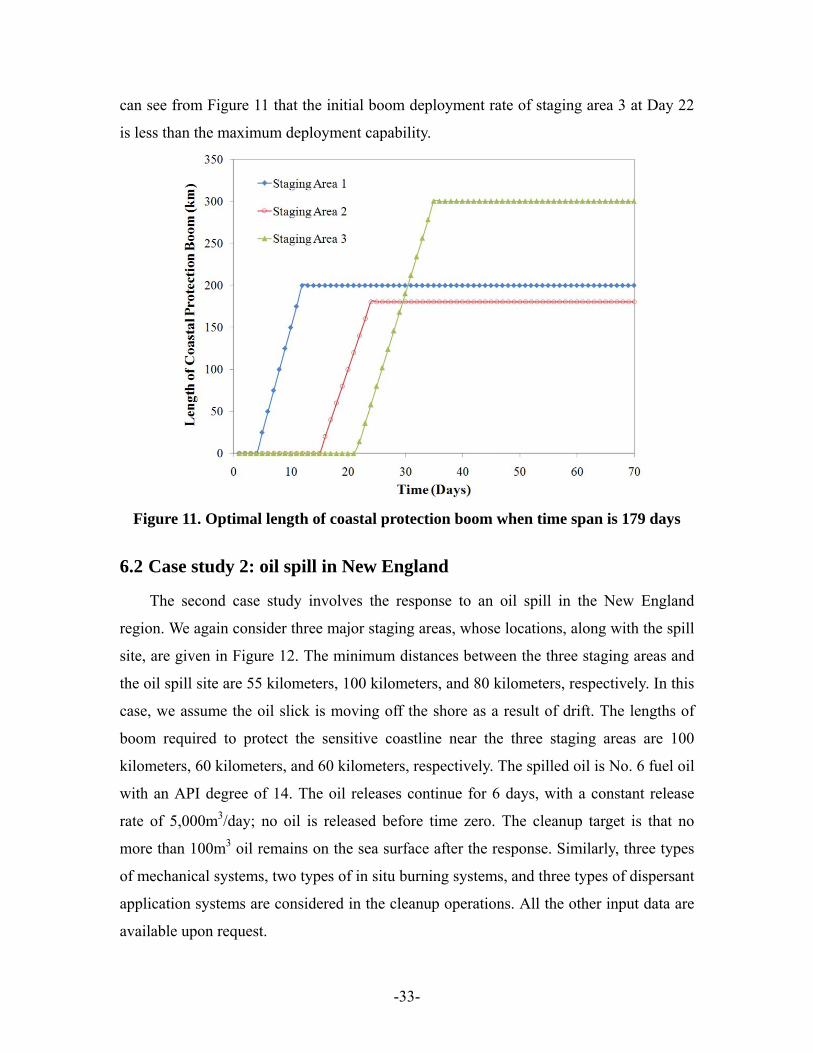
Figure 8. Time trajectories of the oil volumes removed by three methods and

remaining on the sea surface when the time span is 125 days (Point D in Figure 4)

-30-

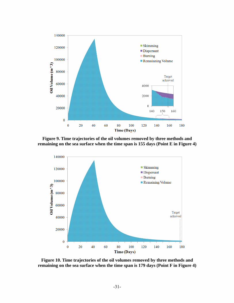
Figure 9. Time trajectories of the oil volumes removed by three methods and

remaining on the sea surface when the time span is 155 days (Point E in Figure 4)

Figure 10. Time trajectories of the oil volumes removed by three methods and

remaining on the sea surface when the time span is 179 days (Point F in Figure 4)

-31-

Figures 5–10 show the time trajectories of the oil volume throughout the response

operations for the six points A–F in Figure 4, where time spans are 75 days, 77 days, 100

days, 125 days, 155 days, and 179 days. We note that the time trajectory of the oil volume

shown in Figure 10 is the same as that for natural weathering, where no cleanup effort

was taken throughout the operations. For all these figures, we can see a similar trend that

the volume of remaining oil first increases from Day 0 to Day 42 and then decreases. The

reason is that the oil was being released at a constant rate to the sea surface before Day 42,

and this release rate is much higher than the removal capability of natural weathering and

all cleanup facilities.

By comparing Figures 5 and 10, however, we can conclude that the maximum volume

of oil on the sea surface can be reduced from around 140,000m3 to around 120,000m3 if

sufficient cleanup efforts are taken in the early stage of the spill. These figures also reveal

that the more cleanup operations are taken, the earlier the cleanup target can be achieved.

Comparison between the three major cleanup methods in terms of the volumes of oil

removed by them shows that dispersant application is usually the most favorable cleanup

approach due of its flexibility in various weather conditions. For the most responsive

instance, however, where a lot of oil needs to be removed by cleanup operations,

skimming becomes as important as dispersant application. Presumably the main reasons

are that the maximum amount of chemical dispersant that can be applied is controlled by

the regulator due to ecological concerns and that skimming has relatively low

requirement of weathering conditions compared to burning. An additional reason is that

mechanical cleanup can gain credit from oil recovery, which in turn reduces the total cost.

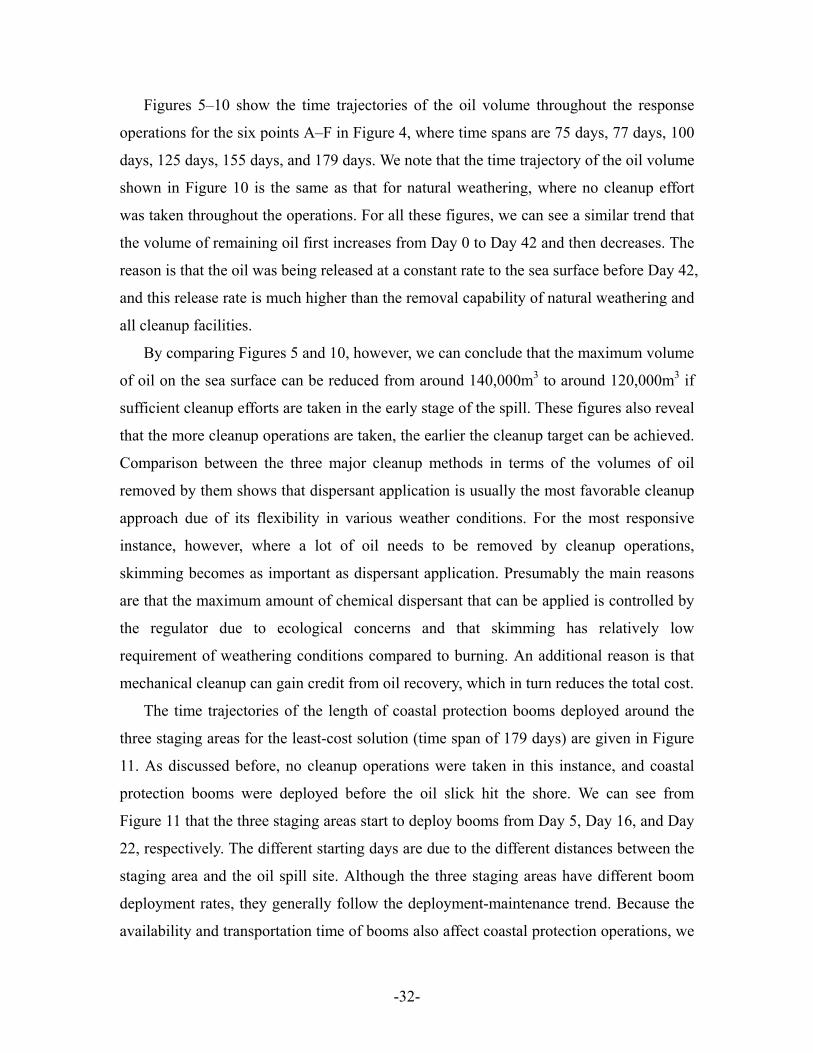
The time trajectories of the length of coastal protection booms deployed around the

three staging areas for the least-cost solution (time span of 179 days) are given in Figure

11. As discussed before, no cleanup operations were taken in this instance, and coastal

protection booms were deployed before the oil slick hit the shore. We can see from

Figure 11 that the three staging areas start to deploy booms from Day 5, Day 16, and Day

22, respectively. The different starting days are due to the different distances between the

staging area and the oil spill site. Although the three staging areas have different boom

deployment rates, they generally follow the deployment-maintenance trend. Because the

availability and transportation time of booms also affect coastal protection operations, we

-32-

can see from Figure 11 that the initial boom deployment rate of staging area 3 at Day 22

is less than the maximum deployment capability.

Figure 11. Optimal length of coastal protection boom when time span is 179 days

6.2 Case study 2: oil spill in New England

The second case study involves the response to an oil spill in the New England

region. We again consider three major staging areas, whose locations, along with the spill

site, are given in Figure 12. The minimum distances between the three staging areas and

the oil spill site are 55 kilometers, 100 kilometers, and 80 kilometers, respectively. In this

case, we assume the oil slick is moving off the shore as a result of drift. The lengths of

boom required to protect the sensitive coastline near the three staging areas are 100

kilometers, 60 kilometers, and 60 kilometers, respectively. The spilled oil is No. 6 fuel oil

with an API degree of 14. The oil releases continue for 6 days, with a constant release

rate of 5,000m3/day; no oil is released before time zero. The cleanup target is that no

more than 100m3 oil remains on the sea surface after the response. Similarly, three types

of mechanical systems, two types of in situ burning systems, and three types of dispersant

application systems are considered in the cleanup operations. All the other input data are

available upon request.

-33-

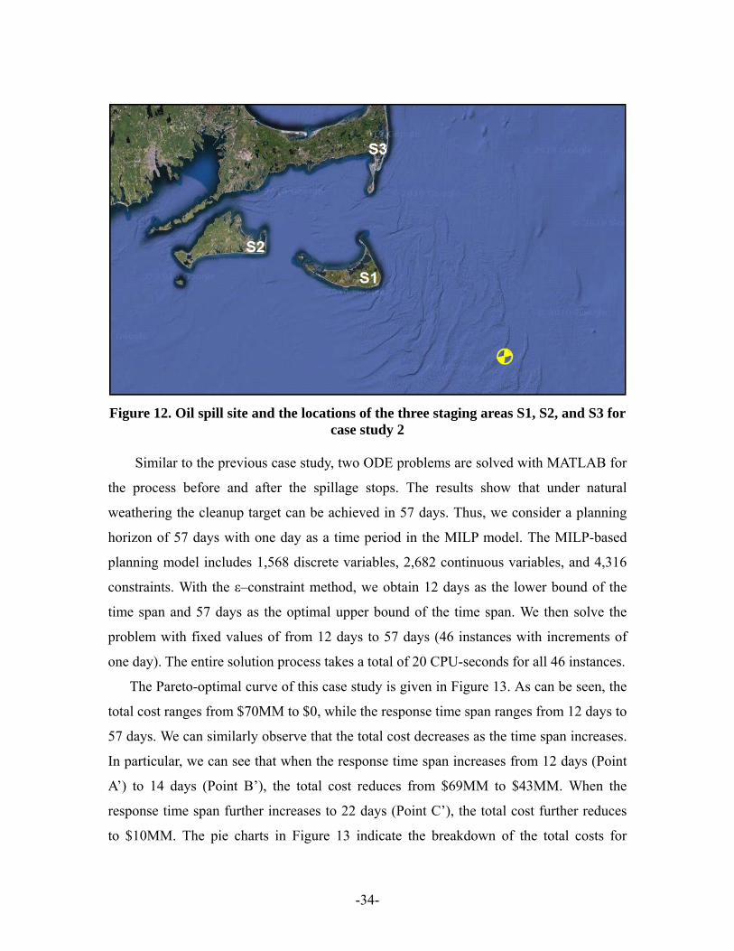
Figure 12. Oil spill site and the locations of the three staging areas S1, S2, and S3 for

case study 2 Similar to the previous case study, two ODE problems are solved with MATLAB for

the process before and after the spillage stops. The results show that under natural

weathering the cleanup target can be achieved in 57 days. Thus, we consider a planning

horizon of 57 days with one day as a time period in the MILP model. The MILP-based

planning model includes 1,568 discrete variables, 2,682 continuous variables, and 4,316

constraints. With the ε–constraint method, we obtain 12 days as the lower bound of the

time span and 57 days as the optimal upper bound of the time span. We then solve the

problem with fixed values of from 12 days to 57 days (46 instances with increments of

one day). The entire solution process takes a total of 20 CPU-seconds for all 46 instances.

The Pareto-optimal curve of this case study is given in Figure 13. As can be seen, the

total cost ranges from $70MM to $0, while the response time span ranges from 12 days to

57 days. We can similarly observe that the total cost decreases as the time span increases.

In particular, we can see that when the response time span increases from 12 days (Point

A’) to 14 days (Point B’), the total cost reduces from $69MM to $43MM. When the

response time span further increases to 22 days (Point C’), the total cost further reduces

to $10MM. The pie charts in Figure 13 indicate the breakdown of the total costs for

-34-

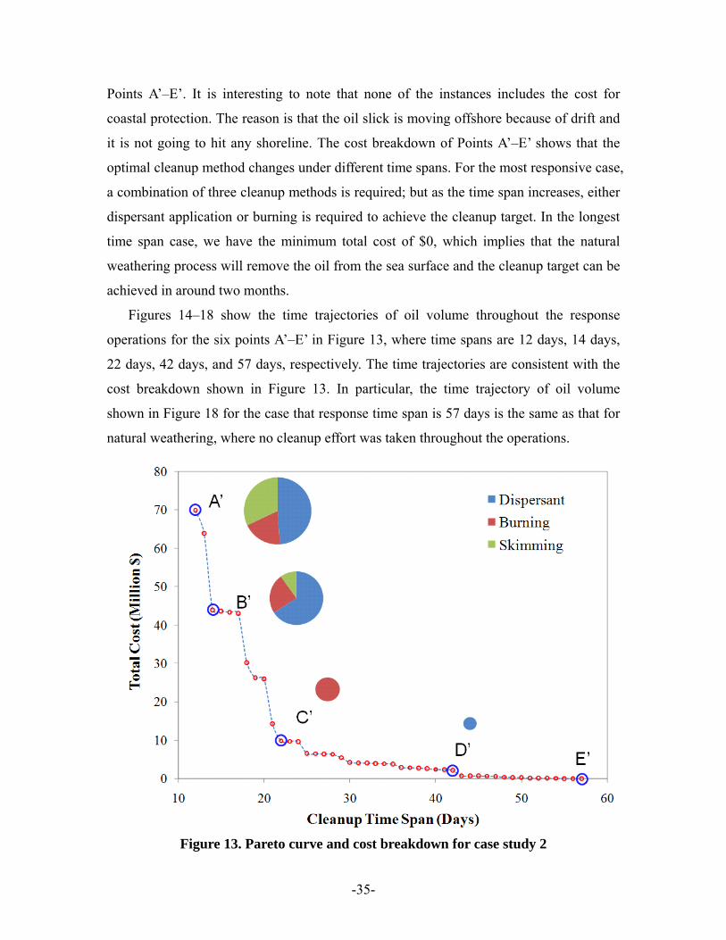
Points A’–E’. It is interesting to note that none of the instances includes the cost for

coastal protection. The reason is that the oil slick is moving offshore because of drift and

it is not going to hit any shoreline. The cost breakdown of Points A’–E’ shows that the

optimal cleanup method changes under different time spans. For the most responsive case,

a combination of three cleanup methods is required; but as the time span increases, either

dispersant application or burning is required to achieve the cleanup target. In the longest

time span case, we have the minimum total cost of $0, which implies that the natural

weathering process will remove the oil from the sea surface and the cleanup target can be

achieved in around two months.

Figures 14–18 show the time trajectories of oil volume throughout the response

operations for the six points A’–E’ in Figure 13, where time spans are 12 days, 14 days,

22 days, 42 days, and 57 days, respectively. The time trajectories are consistent with the

cost breakdown shown in Figure 13. In particular, the time trajectory of oil volume

shown in Figure 18 for the case that response time span is 57 days is the same as that for

natural weathering, where no cleanup effort was taken throughout the operations.

Figure 13. Pareto curve and cost breakdown for case study 2

-35-

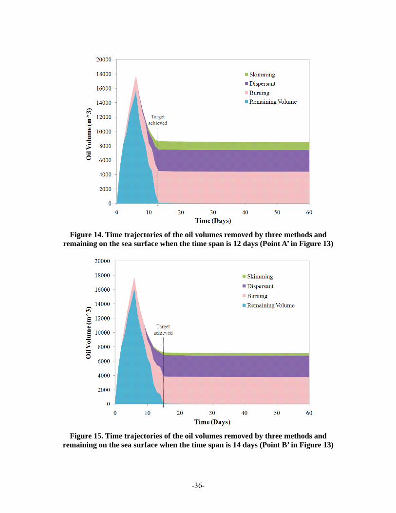
Figure 14. Time trajectories of the oil volumes removed by three methods and

remaining on the sea surface when the time span is 12 days (Point A’ in Figure 13)

Figure 15. Time trajectories of the oil volumes removed by three methods and

remaining on the sea surface when the time span is 14 days (Point B’ in Figure 13)

-36-

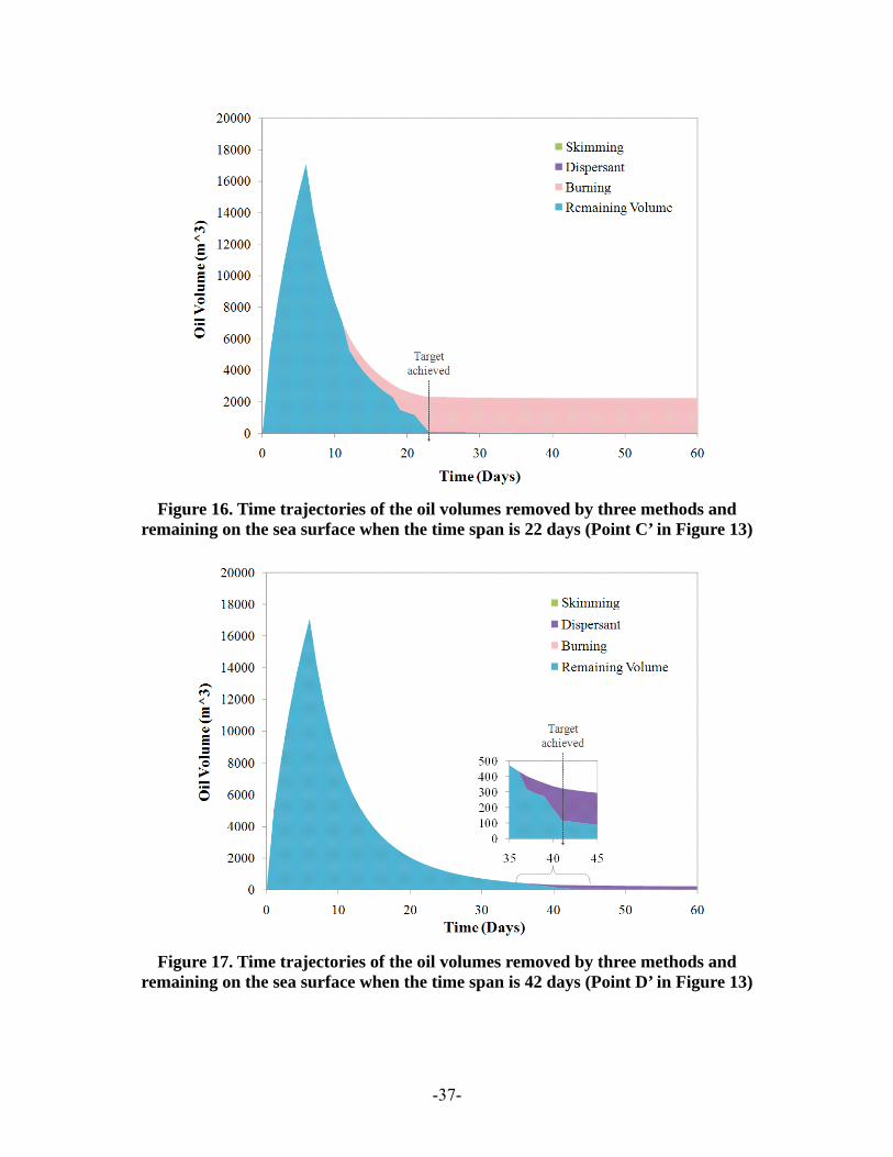
Figure 16. Time trajectories of the oil volumes removed by three methods and

remaining on the sea surface when the time span is 22 days (Point C’ in Figure 13)

Figure 17. Time trajectories of the oil volumes removed by three methods and

remaining on the sea surface when the time span is 42 days (Point D’ in Figure 13)

-37-

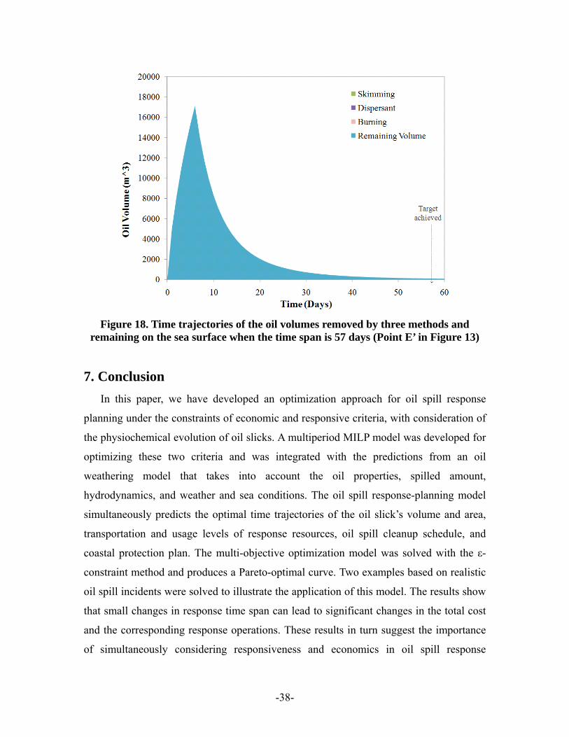
Figure 18. Time trajectories of the oil volumes removed by three methods and

remaining on the sea surface when the time span is 57 days (Point E’ in Figure 13)

7. Conclusion In this paper, we have developed an optimization approach for oil spill response

planning under the constraints of economic and responsive criteria, with consideration of

the physiochemical evolution of oil slicks. A multiperiod MILP model was developed for

optimizing these two criteria and was integrated with the predictions from an oil

weathering model that takes into account the oil properties, spilled amount,

hydrodynamics, and weather and sea conditions. The oil spill response-planning model

simultaneously predicts the optimal time trajectories of the oil slick’s volume and area,

transportation and usage levels of response resources, oil spill cleanup schedule, and

coastal protection plan. The multi-objective optimization model was solved with the ε-

constraint method and produces a Pareto-optimal curve. Two examples based on realistic

oil spill incidents were solved to illustrate the application of this model. The results show

that small changes in response time span can lead to significant changes in the total cost

and the corresponding response operations. These results in turn suggest the importance

of simultaneously considering responsiveness and economics in oil spill response

-38-

planning.

A future extension of this research is to develop a mixed-integer dynamic

optimization (MIDO) approach that seamlessly integrates the planning model with the oil

weathering model. The solution of the resulting MIDO model is a nontrivial task and may

require an initialization step based on the approach proposed in this work.

Acknowledgment This research is supported by the U.S. Department of Energy under contract DE-

AC02-06CH11357.

Appendix: Oil Transport and Weathering Model In the oil transport and weathering process, a variety of complex physical, chemical

and biological phenomena take place simultaneously. The weathering process depends on

the initial oil properties, the spilled amount, hydrodynamics, and weather conditions. All

these factors vary with time. Thus, it is usually nontrivial to determine the weathering

process of the spilled oil and the subsequent consequences. It is estimated that over 50 oil

weathering models, based mainly on empirical and semi-empirical approaches, have been

developed (Brebbia, 2001; Buchanan & Hurford, 1988; D. Mackay & McAuliffe, 1988;

Reed et al., 1999; Sebastiao & Sores, 1995; Spaulding, 1988). Although any oil

weathering model can, in principle, be used in the approach proposed in this paper, we

present in this section an ODE model for the dynamic oil transport and weathering

processes that predicts important parameters, such as time trajectories of the oil volume,

spill size, and other basic oil properties (e.g., viscosity and water content), for the

proposed response planning model. A list is given in the nomenclature section.

A.1 Spreading

The dominant processes that cause significant short-term changes in oil

characteristics are spreading, evaporation, dispersion and emulsification. They all occur

progressively at different rates depending on the oil properties and the weather condition.

Spreading of oil released on water is probably the most dominant process of a spill,

-39-

because it strongly influences other weathering processes such as evaporation and

dispersion. Due to the gravity and surface tension, oils spilled on the surface of sea

usually spread like a thin continuous layer with a circular pattern. The spreading process

includes three phases (Fay, 1969). The first phase is the gravity-inertial spreading which

lasts for very short time period (minutes to hours). The second phase, which covers the

planning horizon of oil spill response in most cases, is attributed to combined gravity and

viscosity phenomena. The third phase, the tension-viscous phase, occurs when the Oil

slick is sufficiently thin due to weathering and broken into a few separated slicks.

Therefore, most models consider mainly the second phase, known as the gravity-viscous

spreading, for the simulation of spreading.

The rate of change of slick area for the second phase can be modeled with equation

(38), which is widely used for oil spill models with multiple variables changing

simultaneously (Mackay et al., 1980; Reed et al., 1999; Sebastiao & Sores, 1995;

Spaulding, 1988).

1 4/31

dA K A Vdt

−= (38)

where A is the surface area of oil slick (m2), V is the volume of oil (m3), and K1 is the

dominant physicochemical parameters of the crude oil in the gravity-viscous spreading

process with default value of 150 s-1 (Mackay et al., 1980). As reported by CONCAWE

(1983), the spreading behavior of two crude oils with almost comparable spreading

coefficients but with a considerable difference in other properties is usually very similar.

The initial area of oil slick, A0 (m2) can be determined by the gravity-viscous

formulation as follows (Fay, 1969):

( ) 1/65402

0 23

w o

w w

gVkAk v

ρ ρπ

ρ⎡ ⎤−

= ⎢⎣ ⎦

⎥ (39)

where g is the acceleration of gravity (mÿs-2), wρ is the density of seawater, oρ is the

density of fresh oil, is the kinematic viscosity of seawater (0.801ÿ10-6 m2s-1 under

30oC), V0 is the initial volume of the oil slick (spilled before time 0), t refers to time (s)

and k2 and k3 are constants with values of 1.21 and 1.53, respectively (NOAA, 2000).

wv

-40-

A.2 Evaporation

Evaporation is the primary initial process involved in the removal of oil from sea. The

rate of evaporation is determined by the physicochemical properties of the oil and is

increased by spreading, high water temperature, strong wind, and rough sea. By

evaporation, low boiling components will rapidly be removed, thus reducing the volume

of the remaining slick.

The rate that oil evaporates from the sea surface is modeled by the following equation

(D. Mackay & Matsugu, 1973; Stiver & Mackay, 1984),

(expE ev evev o G E

K

dF K A BA T T Fdt V T

⎛ ⎞= − +⎜

⎝ ⎠)⎟

.78

, (40)

where FE is the volume fraction of oil that has been evaporated until time t, TK is the oil

temperature (K), and Aev and Bev are empirical constants with fixed values of 6.3 and 10.3,

respectively (NOAA, 2000). Kev is the mass transfer coefficient for evaporation (ms-1)

and can be calculated by (Buchanan & Hurford, 1988), 3 02.5 10evK WIND−= × ,

where WIND is the wind speed (ms-1). TO and TG are the initial boiling point and the

gradient of the oil distillation curve, respectively. Their values can be obtained from the

distillation curve of the specific oil spilled or can be calculated through functions of the

oil API (American Petroleum Institute) degree as follows (NOAA, 2000):

457.16 3.3447 APIOT = − ⋅ ( ) 1356.7 247.36 ln APIGT = − ⋅

At the beginning of the evaporation process, none of the oil has been evaporated.

Thus, initial value of evaporative fraction at time 0 is set as zero.

( )0 0E tF = = (41)

A.3 Emulsification

In emulsification, water droplets are entrained in the oil. This process results in

significant changes in multiple physicochemical properties of oil slicks, such as viscosity.

Crude oil will emulsify when the asphaltene content is higher than 5 mass percent of the

-41-

spilled oil. The dynamic emulsification process that incorporates water into oil can be

computed with the following equation (Mackay et al., 1980):

( )2

3

1 1Wem

dY YK WINDdt C

⎛ ⎞= ⋅ + ⋅ −⎜

⎝ ⎠W ⎟

, (42)

where is the fractional water content in the emulsion, C3 is a viscosity constant for

the final fraction water content (~0.7 for crude oils), and is an empirical constant

between 1 x 10-6 and 2 x 10-6.

WY

emK

Similar to the initial condition of evaporation process, the fractional water content at

beginning of emulsification process is zero.

( )0 0W tY = = (43)

As a result of both Mousse formation and evaporation, the viscosity of oil slick may

significantly increase during the emulsification process. The rate of changes in viscosity

is given by (Mackay & McAuliffe, 1988; Mooney, 1951):

( ) 423

2.51

W E

W

d dY Cdt dt dtC Y

dFμ μ μ= +− ,

(44)

where μ is the viscosity of oil slickand C4 is an oil-dependent constant equal to 10 for

crude oils (Mackay et al., 1980; Sebastiao & Sores, 1995). Note that the first term in (44)

corresponds to the Mooney equation for the viscosity increment rate due to Mousse

formation, and the second term is the contribution by evaporation.

The initial value of the viscosity is the same as that of the parent oil viscosity, which

can be calculated by the following equation (Buchanan & Hurford, 1988):

0 224 ACμ = × ,

(45)

where AC is the asphaltene content (%) of the parent oil.

A.4 Dispersion

Natural dispersion of crude oils after spillage at sea is the process of forming small

droplets of oil to be transferred in the water column. Natural dispersion may account for a

significant part of removal of oil from the sea surface in addition to evaporation. Besides

the total volume of oil on the sea surface and the slick area, an important parameter

-42-

influencing natural dispersion is the oil/water interfacial tension, which affects

globulation and coalescence, as well as the transport (dispersion) of oil droplets into the

water column. The viscosity of the spilled oil also affects natural dispersion - the more

viscous the oil is, the lower its ability to form oil droplets.

In this work, we use the approach proposed by Mackay et al. (1980) and Sebastiao &

Sores (1995) to calculate the rate of dispersion into the water column of floating oil slick

at the sea. The formulation is given as follows:

( )2

1/ 2

0.11 150

D

t

WIND A VdVdt A Vζ μ

⋅ + ⋅=

+ ⋅ ⋅⋅

, (46)

where VD is volume of oil naturally diepersed and tζ is the oil-water interfacial tension.

The initial value of the volume of oil that is naturally dispersed is zero.

( )0 0D tV = = (47)

A.5 Volume balance

Oil escapes from the surface slick by two major processes: evaporation and dispersion.

As can be seen from Equations (40) and (46), these two processes depend on the slick

surface, which changes over time due to spreading. Emulsification not only changes the

viscosity of oil slick and affects the dispersion process but also results in the degradation

of the cleanup capability of skimmers discussed earlier. The volume balance of the oil

slick is based on the volume variation rate given by (Sebastiao & Sores, 1995):

E DdV dF dVVdt dt dt

= − − +VI ,

(48)

where the first term on the right-hand side is for the evaporation rate; the second term is

for natural dispersion; and the third term, VI, is a time-dependent parameter of the oil

spill rate. Most oil spill models consider two release types of oil spillage: the

instantaneous release mode, which is for oil spilled in an hour or less, and the continuous

release mode for oil spilled into the water over a given time duration with a fixed spill

rate. If we define tf1 as the time when the oil spillage stops and tf2 as the final time of the

planning horizon, then the time-dependent parameter VI is given by the following

expression:

-43-

constat spill rate, 0 10, 1 2

t tfVI

tf t tf≤ ≤⎧

= ⎨ ≤ ≤⎩ (49)

The initial volume of oil slick is given as V0, .

( ) 00tV = =V (50)

Note that we have tf1 = 0 in the instataneous release type; that is, VI = 0 over the planning

horizon but V0 is nonzero.

A.6 Solution method

The oil weathering model is a system of differential equations consisting of equations

(38), (40), (42), (44), (46), and (48). Numerical solution of this model can be obtained by

using the Runge-Kutta method. Because of the time-dependent oil spill rate VI, two ODE

systems might need to be solved. The first problem is for the period that oil is spilling

with a constant release rate, namely, from time 0 to tf1. The initial conditions of this

problem are given in (39), (41), (43), (45), (47), and (50). The second problem is for the

period from the oil spillage stops to the end of the planning horizon, namely, from tf1 to

tf2. The solution of the first ODE problem (i.e., the values of oil slick area A, volume V,

evaporative volume fraction FE, water content , oil slick viscosity WY μ , and naturally

diepersed volume of oil VD) at the final time tf1 is used as the initial condition of the

second ODE. The solution of the oil weathering model provides time trajectories of

important physical and chemical parameters of the oil slicks.

Nomenclature

Nomenclature for the planning model

Sets/Indices

B: Set of in situ burning response system types indexed by b

D: Set of chemical dispersant application system types indexed by d

I: Set of staging areas (including airlift wing stations) indexed by i

J: Set of containment boom storage/supplier locations indexed by j

K: Set of dispersant supplier locations indexed by k

-44-

M: Set of skimming (mechanical cleanup & recovery) system types indexed by m

T: Set of time periods indexed by t, t’

Parameters

,i tAREA : The expected slick area that the oil slick would hit the shore around staging

area i at time period t if no boom in this area was deployed for protection

iBDU : Maximum deployment rate of boom in staging area i at time period t

iBDL : Minimum deployment rate of boom in staging area i at time period t

jBA : Available amount of coastal protection booms from storage location j

, ,boomi j tBTU : Maximum transportation amount of coastal protection booms from storage

location j to staging area i at time period t

, ,Mi m tC : Operating cost of mechanical cleanup and recovery system m dispatched from

staging area i at time t

, ,Bi b tC : Operating cost of in situ burning system type b from staging area i at time t

, ,Di d tC : Cost of dispatching a chemical dispersant application system d from staging

area i at time t to spray a full-load dispersant

,boomi tCBM : Maintenance cost unit length coastal protection boom in staging area i at time t

,boom

i tCDEP :Cost of deploying unit length of coastal protection boom in staging area i

,k tCDS : Amount of chemical dispersant available in supplier location k at time period t

dispersantiCI : Unit inventory holding cost of chemical dispersant in staging area i at time t

boomiCI : Unit inventory holding cost of boom in staging area i at time t

,boom

i jCT : Staging and transportation costs of unit length coastal protection booms from

storage location j to staging area i

,dispersant

i kCT : Purchase and transportation costs of unit volume chemical dispersant from

supplier location k to staging area i

DLIMIT : Maximum amount of dispersant that can be applied in the cleanup

,Mi mFC : Fixed cost (including mobilization, equipment transportation, and set-up costs)

of staging mechanical cleanup and recovery system m dispatched to staging

-45-

area i

,Bi bFC : Fixed cost (including mobilization, equipment transportation, and set-up costs)

of staging in situ burning response system type b to staging area i

,Di dFC : Fixed cost (including mobilization, spray system transportation and system set-

up costs) of staging chemical dispersant application system d to staging area i

,boomi tFCBM : Fixed cost of maintaining booms in staging area i at time period t

,boom

i tFCDEP : Fixed cost of deploying boom in staging area i at time period t

tH : Length of time period t

iL : Length of boom required to protect the shore around staging area i

,Bi bN : Available number of in situ burning response system type b that can be

dispatched from staging area i

,Di dN : Available number of chemical dispersant application system types d that can be

dispatched from staging area i

,Mi mN : Available number of mechanic cleanup and recovery system type m that can be

dispatched from staging area i

OC : Unit price of recovered oil

bTHICK : Minimum slick thickness that in situ burning response system b can operate

,Bi bQ : Operating capability of in-situ burning system type b from staging area i

,Di dQ : Full0load capacity of dispersant application system d from staging area i

,Mi mQ : Operating capability of mechanical cleanup system m from staging area i

U : A sufficiently large number

V0: Initial volume of oil spilled at time 0

tVI : Volume of oil that was newly released to the sea surface at time t

V : Cleanup target, maximum volume of oil left on the sea surface after cleanup effecttρ : Effectiveness factor (ratio between oil dispersed and dispersant sprayed) for

chemical dispersant application operation at time t accuracydρ : Accuracy factor (percentage of sprayed dispersant that can reach oil slick) of

-46-

chemical dispersant application system d

,boomi jτ : Transportation time of boom from storage location j to staging area i

,dispersanti kτ : Transportation time of dispersant from supplier location k to staging area i

,B

i bλ : Total response time of in situ burning response system type b dispatched from

staging area i (including the times to notify, mobilize, dispatch, and deploy the

system)

,D

i dλ : Total response time of chemical dispersant application system types d

dispatched from staging area i (including the times to notify, mobilize, dispatch,

and deploy the system)

,Mi mλ : Total response time of mechanic cleanup and recovery system type m

dispatched from staging area i (including the times to notify, mobilize, dispatch

and deploy the system) Mtω : Weather factor for mechanic cleanup and recovery operation at time t

Btω : Weather factor for controlled burning operation at time t

Dtω : Weather factor for chemical dispersant application operation at time t

,Boomi tω : Weather factor for maintaining booms in staging area i at time t

, ,i d tγ : Maximum number of sorties of dispersant application system types d from

staging area i to oil spill site in time period t

iϕ : Lifetime before failure for containment booms deployed at staging area i

tη : Percentage of oil that can be recovered in the emulsified oil collected at time t

tδ : Thickness of oil slick at the end of time period t

tθ : Percentage of oil removed from the sea surface due to evaporation and natural

dispersion at time t

Integer Variables

tf : 0-1 variable. Equal to 1 if cleanup target is not achieved at the end of time

period t

-47-

, ,Mi m tx : Number of mechanical cleanup and recovery system m from staging area i

operating on scene at time period t

, ,Bi b tx : Number of in situ burning response system b from staging area i operating on

scene at time period t

, ,Di d tx : Number of sorties of chemical dispersant application systems d dispatched

from staging area i at time period t to spray dispersants

, ,Mi m ty : Number of mechanical cleanup and recovery system m notified at time period t

to be staged at staging area i

, ,Bi b ty : Number of in situ burning response system b notified at time period t to be

staged at staging area i

, ,Di d ty : Number of chemical dispersant application systems d notified at time period t

to be staged at staging area i

,i tzd : 0-1 variable. Equal to 1 if boom is being deployed around staging area i to

protect the nearby shoreline at time period t

,i tz : 0-1 variable. Equal to 1 if the shoreline around staging area i is protected by

boom

,i tzm : 0-1 variable, but can be relaxed as a continuous variable. Equal to 1 if

maintenance is required for boom around staging area i

Continuous Variables (0 to ) +∞

tarea : Area of oil slick on the surface at the end of time t

,i tbdep : Amount of coastal protection booms deployed in staging area i at time period t

,i tbfail : Amount of coastal protection booms failed in staging area i at time period t

,i tbinv : Length of available boom in staging area i at the end of time period t

,i tbl : Length of coastal protection boom deployed along the shore of staging area i at

the end of time period t

, ,i j tbtr : Amount of coastal protection booms shipped from storage location j to staging

area i at the beginning of time period t

-48-

,i tdinv : Amount of chemical dispersant in staging area i at the end of time period t

, ,i k tdtr : Amount of chemical dispersant shipped from supplier location k to staging area

i at the beginning of time period t Mtu : Volume of oil collected and recovered through mechanical systems at time t

Btu : Volume of oil removed by in situ burning at time period t

Dtu : Volume of oil dispersed due to chemical dispersant application at time period t

tv : Volume of oil on the surface at the end of time t

Nomenclature for the ODE model

A: Area of oil slick (m2)

Aev: Constant for oil weathering process

A0: Initial area of slick (m2)

AC: Asphaltene content (%) of the parent oil

Bev: Constant for oil weathering process

C3: Constant for oil weathering process

C4: Constant for oil weathering process

FE: Fraction of oil evaporated

g: Acceleration of gravity (ms-2)

K1: Constant for oil weathering process

k2: Constant for oil weathering process

k3: Constant for oil weathering process

Kev: Constant for oil weathering process

tf1: Time when the oil spillage stops (release duration)

tf2: Time at the end of the planning horizon (final time of the simulation)

TG: Gradient of the oil distillation curve

TK: Temperature (K)

TO: Initial boiling point of oil

V: Volume of oil slick (m3)

V0: Initial volume of oil spilled before time 0

VD: Volume of oil naturally diepersed

-49-

VI: Time-dependent oil spilled rate

WIND: Wind speed

WY : Fraction of water content in the emulsion

wv : Kinematic viscosity of seawater

wρ : Seawater density

oρ : Oil density

μ : Viscosity of oil slick

0μ : Viscosity of parent oil

tζ : Oil-water interfacial tension (dyne/m)

References Bojarski, A. D., Laínez, J. M., Espuña, A., & Puigjaner, L. (2009). Incorporating

environmental impacts and regulations in a holistic supply chains modeling: An LCA approach. Computers & Chemical Engineering, 33, 1747-1759.

Brebbia, C. A. (2001). Oil spill modeling and processes. UK: WIT Press. Buchanan, I., & Hurford, N. (1988). Methods for predicting the physical changes in oil

spilt at sea. Oil & Chemical Pollution, 4, 311-328. CONCAWE. (1983). Characteristics of petroleum and its behavior at sea. In (Vol. Report

No. 8/83). Dua, V., & Pistikopoulos, E. N. (2004). Parametric optimization in process systems

engineering: theory and algorithms. Proceeding of Indian National Science Academy, 69A, 429-444.

Duque, J., Barbosa-Povoa, A. P. F. D., & Novais, A. Q. (2010). Design and planning of sustainable industrial networks: application to a recovery network of residual products. Industrial & Engineering Chemistry Research, 49, 4230-4248.

Fay, J. A. (1969). The spread of Oil Slicks on a Calm Sea. In D.-P. Hoult (Ed.), Oil on the sea (pp. 53-63). New York: Plenum Press.

Fingas, M. (2001). The basics of oil spill cleanup. New York: Lewis. Gatica, G., Papageorgiou, L. G., & Shah, N. (2003). Capacity planning under uncertainty

for the pharmaceutical industry. Chemical Engineering Research & Design, 81, 665-678.

Gkonis, K. G., Kakalis, N. M. P., Ventikos, N. P., Ventikos, Y., & Psaraftis, H. N. (2007). A model-based approach for tactical decision making in oil spill response. In International Symposium on Maritime Safety, Security & Eenviromental Protection. Athens, Greece.

Guillen-Gosalbez, G., & Grossmann, I. E. (2009). Optimal design and planning of sustainable chemical supply chains under uncertainty. AIChE Journal, 55, 99-121.

Iakovou, E., Douligeris, C., & Korde, A. (1994). A synthesis of decision analysis,

-50-

assessment, and planning for oil spill models for contingency incidents. Omega, 22, 457-470.

Ierapetritou, M. G., & Pistikopoulos, E. N. (1994). Simultaneous incorporation of flexibility and economic risk in operational planning under uncertainty. Computers & Chemical Engineering, 18, 163-189

Kallrath, J. (2002). Planning and scheduling in the process industry. OR Spectrum, 24, 219-250.

Laird, C. D., Biegler, L. T., & Waanders, B. G. V. B. (2006). Mixed-integer approach for obtaining unique solutions in source inversion of water networks,. Journal Of Water Resources Planning And Management-ASCE, 132, 242-251.

Mackay, D., Buist, I. A., Mascarenhas, R., & Paterson, S. (1980). Oil spill processes and models: Environment Canada Manuscript Report No 8. EE-8, . In. Ottawa, Ontario.

Mackay, D., & Matsugu, R. (1973). Evaporation rate of liquid hydrocarbon spills on land and water. Canadian Journal of Chemical Engineeirng, 51, 434-439.

Mackay, D., & McAuliffe, C. D. (1988). Fate of hydrocarbons discharged at sea. Oil & Chemical Pollution, 5, 1-20.

Maravelias, C. T., & Grossmann, I. E. (2001). Simultaneous planning for new product development and batch manufacturing facilities. Industrial & Engineering Chemistry Research, 40, 6147-6164.

Michel, J., Adams, E. E., Addassi, Y., Copeland, T., Greeley, M., James, B., Mcgee, B., Mitchelmore, C., Onishi, Y., Payne, J., Salt, D., & Wrenn, B. (2005). Oil spill dispersants: efficacy and effects. Washington, DC: National Academies Press.

Mooney, M. (1951). The viscosity of a concentrated suspension of spherical particles. Journal of Colloid Science, 6, 162-170.

Neiro, S. M. S., & Pinto, J. M. (2005). Multiperiod optimization for production planning of petroleum refineries. . Chemical Engineering Communications, 192, 62-88.

Nemhauser, G. L., & Wolsey, L. A. (1988). Integer and combinatorial optimization. New York, NY: John Wiley and Son Inc.

NOAA. (1992). Oil spill case histories 1967-1991: summaries of significant U.S. and international spills. In. Seattle, Washington.

NOAA. (2000). ADIOS 2. In. Seattle, Wa: National Oceanic and Atmospheric Administration.

Ornitz, B., & Champ, M. (2003). Oil spills first principles: prevention and best response. Netherlands: Elsevier.

Psaraftis, H. N., & Ziogas, B. (1985). A tactical decision algorithm for the optimal dispatching of oil spill cleanup equipment. Management Science, 31, 1475-1491.

Raman, R., & Grossmann, I. E. (1993). Symbolic integration of logic in mixed integer linear programming techniques for process synthesis. Computers & Chemical Engineering, 27, 909.

Reed, M., Johansen, I., Brandvik, P. J., Daling, P., Alun Lewisà, Fioccoà, R., Mackay, D., & Prentki, R. (1999). Oil spill modeling towards the close of the 20th century: overview of the state of the art. Spill Science & Technology Bulletin, 5, 3-16.

Reklaitis, G. V. (2000). Overview of planning and scheduling technologies. Latin American Applied Research, 30, 285-293.

Rodera, H., Bagajewicz, M. J., & Trafalis, T. B. (2002). Mixed-integer multiobjective

-51-

-52-

process planning under uncertainty. Industrial & Engineering Chemistry Research, 41, 4075-4084.

Sebastiao, P., & Sores, C. G. (1995). Modeling the fate of oil spills at sea. Spill Science & Technology Bulletin, 2, 121-131.

Spaulding, M. L. (1988). A state-of-the-art review of oil spill trajectory and fate modeling. Oil & Chemical Pollution, 4, 39-55.

Srinivasa, A. V., & Wilhelm, W. E. (1997). A procedure for optimizing tactical response in oil spill clean up operations. European Journal of Operational Research, 102, 554-574.

Stiver, W., & Mackay, D. (1984). Evaporation rate of spills of hydrocarbons and petroleum mixtures. Environmental Science & Technology, 18, 834-840.

Verderame, P. M., Elia, J. A., & Floudas, C. A. (2010). Planning and scheduling under uncertainty: a review across multiple sectors. Industrial & Engineering Chemistry Research, 49, 3993-4017.

Verderame, P. M., & Floudas, C. A. (2009). Operational planning framework for multisite production and distribution networks. Computers & Chemical Engineering, 33, 1036-1050.

Wilhelm, W. E., & Srinivasa, A. V. (1997). Prescribing tactical response for oil spill clean up operations. Management Science, 43, 386-402.

You, F., & Grossmann, I. E. (2008). Design of responsive supply chains under demand uncertainty. Computers & Chemical Engineering, 32, 2839-3274.

You, F., & Grossmann, I. E. (2009). Balancing responsiveness and economics in the design of process supply chains with multi-echelon stochastic inventory. AIChE Journal, In press, DOI: 10.1002/aic.12244.

You, F., & Grossmann, I. E. (2010). Stochastic inventory management for tactical process planning under uncertainties: MINLP model and algorithms. AIChE Journal, In press, DOI: 10.1002/aic.12338.

You, F., Grossmann, I. E., Pinto, J. M., & Megan, L. (2010). Optimal distribution-inventory planning of industrial gases: II. Minlp models and algorithms for stochastic cases. Industrial & Engineering Chemistry Research, Submitted.

You, F., Wassick, J. M., & Grossmann, I. E. (2009). Risk management for global supply chain planning under uncertainty: models and algorithms. AIChE Journal, 55, 931-946.

The submitted manuscript has been created by UChicago Argonne, LLC, Operator of Argonne National Laboratory ("Argonne"). Argonne, a U.S. Department of Energy Office of Science laboratory, is operated under Contract No. DE-AC02-06CH11357. The U.S. Government retains for itself, and others acting on its behalf, a paid-up nonexclusive, irrevocable worldwide license in said article to reproduce, prepare derivative works, distribute copies to the public, and perform publicly and display publicly, by or on behalf of the Government.