Oil Prices, Exhaustible Resources, and Economic Growth*econweb.ucsd.edu/~jhamilto/handbook_climate.pdf · Oil Prices, Exhaustible Resources, and Economic ... real price of crude petroleum

Oil Prices, Exhaustible Resources, and EconomicGrowth*

James D. Hamilton

Department of Economics

University of California, San Diego

email: [email protected]

October 18, 2011

Revised: October 1, 2012

∗Prepared for Handbook of Energy and Climate Change. I thank Roger Fouquet and

Lutz Kilian for helpful comments on an earlier draft.

1

Abstract

This chapter explores details behind the phenomenal increase in global crude oil produc-

tion over the last century and a half and the implications if that trend should be reversed.

I document that a key feature of the growth in production has been exploitation of new

geographic areas rather than application of better technology to existing sources, and sug-

gest that the end of that era could come soon. The economic dislocations that historically

followed temporary oil supply disruptions are reviewed, and the possible implications of that

experience for what the transition era could look like are explored.

2

1 Oil prices and the economics of resource exhaustion.

One of the most elegant theories in economics is Hotelling’s (1931) characterization of the

price of an exhaustible natural resource. From the perspective of overall social welfare,

production today needs to be balanced against the consideration that, once consumed, the

resource will be unavailable to future generations. One option for society would be to

produce more of the commodity today, invest the current marginal benefits net of extraction

costs in some other form of productive capital, and thereby accumulate benefits over time at

the rate of interest earned on productive capital. An alternative is to save the resource so

it can be used in the future. Optimal use of the resource over time calls for equating these

two returns. This socially optimal plan could be implemented in a competitive equilibrium

if the price of the resource net of marginal production cost rises at the rate of interest. For

such a price path, the owner of the mine is just indifferent between extracting a little bit

more of the resource today or leaving it in the ground to be exploited at higher profit in the

future.

This theory is compelling and elegant, but very hard to reconcile with the observed

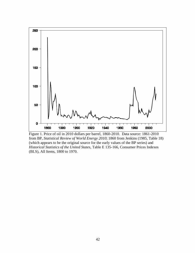
behavior of prices over the first century and a half of the oil industry. Figure 1 plots the

real price of crude petroleum since 1860. Oil has never been as costly as it was at the birth

of the industry. Prior to Edwin Drake’s first oil well in Pennsylvania in 1859, people were

getting illuminants using very expensive methods.1 The term kerosene, which we still use

today to refer to a refined petroleum product, was actually a brand name used in the 1850s

for a liquid manufactured from asphalt or coal, a process which was then, as it still is now,

3

quite expensive.2 Derrick’s Handbook (1898) reported that Drake had no trouble selling all

the oil his well could produce in 1859 at a price of $20/barrel. Given the 24-fold increase

in estimates of consumer prices since 1859, that would correspond to a price in 2010 dollars

a little below $500/barrel. As drillers producing the new-found “rock oil” from other wells

brought more of the product to the market, the price quickly fell, averaging $9.31/barrel for

1860 (the first year shown in Figure 1). In 2010 prices, that corresponds to $232 a barrel,

still far above anything seen subsequently. Even ignoring the initial half-century of the

industry, the price of oil in real terms continued to drop from 1900 to 1970. And despite

episodes of higher prices in the 1970s and 2000s, throughout the period from 1992-1999, the

price of oil in real terms remained below the level reached in 1920.

There are two traditional explanations for why Hotelling’s theory appears to be at odds

with the long-run behavior of crude oil prices. The first is that although oil is in principle

an exhaustible resource, in practice the supply has always been perceived to be so vast,

and the date at which it will finally be exhausted has been thought to be so far into the

future, that finiteness of the resource had essentially no relevance for the current price. This

interpretation could be reconciled with the Hotelling solution if one hypothesizes a tiny rent

accruing to owners of the resource that indeed does grow at the rate of interest, but in

practice has always been sufficiently small that the observed price is practically the same as

the marginal extraction cost.

A second effort to save Hotelling’s theory appeals to the role of technological progress,

which could lower marginal extraction costs (e.g., Slade, 1982), lead to discovery of new fields

4

(Dasgupta and Heal, 1979; Arrow and Chang, 1982), or allow the exploitation of resources

previously thought not to be economically accessible (Pindyck, 1978). In generalizations of

the Hotelling formulation, these can give rise to episodes or long periods in which the real

price of oil is observed to fall, although eventually the price would begin to rise according to

these models. Krautkraemer (1998) has a nice survey of theories of this type and examination

of their empirical success at fitting the observed data.

Although it can sometimes be helpful to think about technological progress in broad,

abstract terms, there is also much insight to be had from looking in some detail at the

specific factors that allowed global oil production to increase almost without interruption

over the last 150 years. For this purpose, I begin by examining some of the long-run trends

in U.S. oil production.

1.1 Oil production in the United States, 1859-2010.

Certainly the technology for extracting oil from beneath the earth’s surface has evolved

profoundly over time. Although Drake’s original well was steam-powered, some of the

early drills were driven through rock by foot power, such as the spring-pole method. The

workers would kick a heavy bit at the end of the rope down into the rock, and spring action

from the compressed pole would lift the bit back up. After some time at this, the drill

would be lifted out and a bucket lowered to bail out the debris. Of course subsequent

years produced rapid advances over these first primitive efforts— better sources of power,

improved casing technology, and vastly superior knowledge of where oil might be found.

5

Other key innovations included the adoption of rotary drilling at the turn of the century,

in which circulating fluid lifted debris out of the hole, and secondary recovery methods first

developed in the 1920s, in which water, air, or gas is injected into oil wells to repressurize

the reservoir and allow more of the oil to be lifted to the surface.

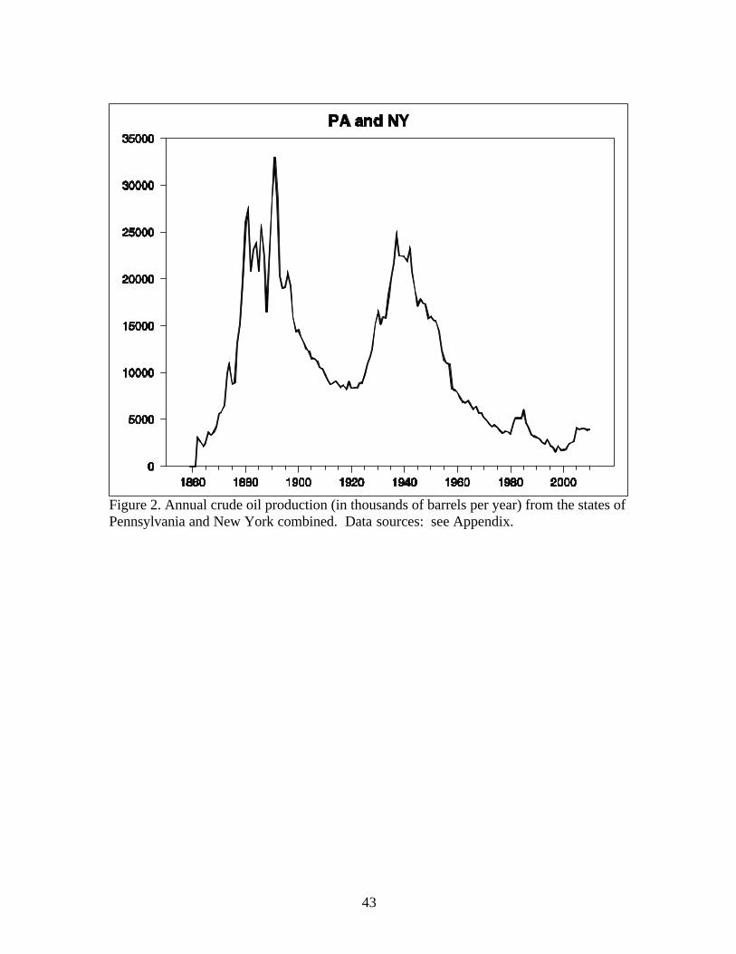
Figure 2 plots the annual oil production levels for Pennsylvania and New York, where

the industry began, from 1862 to 2010. Production increased by a factor of 10 between

1862 and 1891. However, it is a mistake to view this as the result of application of better

technology to the initially exploited fields. Production from the original Oil Creek District

in fact peaked in 1874 (Williamson and Daum, 1959, p. 378). The production gains instead

came primarily from development of new fields, most importantly the Bradford field near

the Pennsylvania-New York border, but also from Butler, Clarion, and Armstrong Counties.

Nevertheless, it is unquestionably the case that better drilling techniques than used in Oil

Creek were necessary in order to reach the greater depths of the Bradford formation.

One also sees quite clearly in Figure 2 the benefits of the secondary recovery methods

applied in the 1920s, which succeeded in producing much additional oil from the Bradford

formation and elsewhere in the state. However, it is worth noting that these methods never

lifted production in Pennsylvania back to where it had been in 1891. In 2010— with the

truly awesome technological advances of the century and a half since the industry began,

and with the price of oil 5 times as high (in real terms) as it had been in 1891— Pennsylvania

and New York produced under 4 million barrels of crude oil. That’s only 12% of what had

been produced in 1891— 120 years ago— and about the level that the sturdy farmers with

6

their spring-poles were getting out of the ground back in 1868.

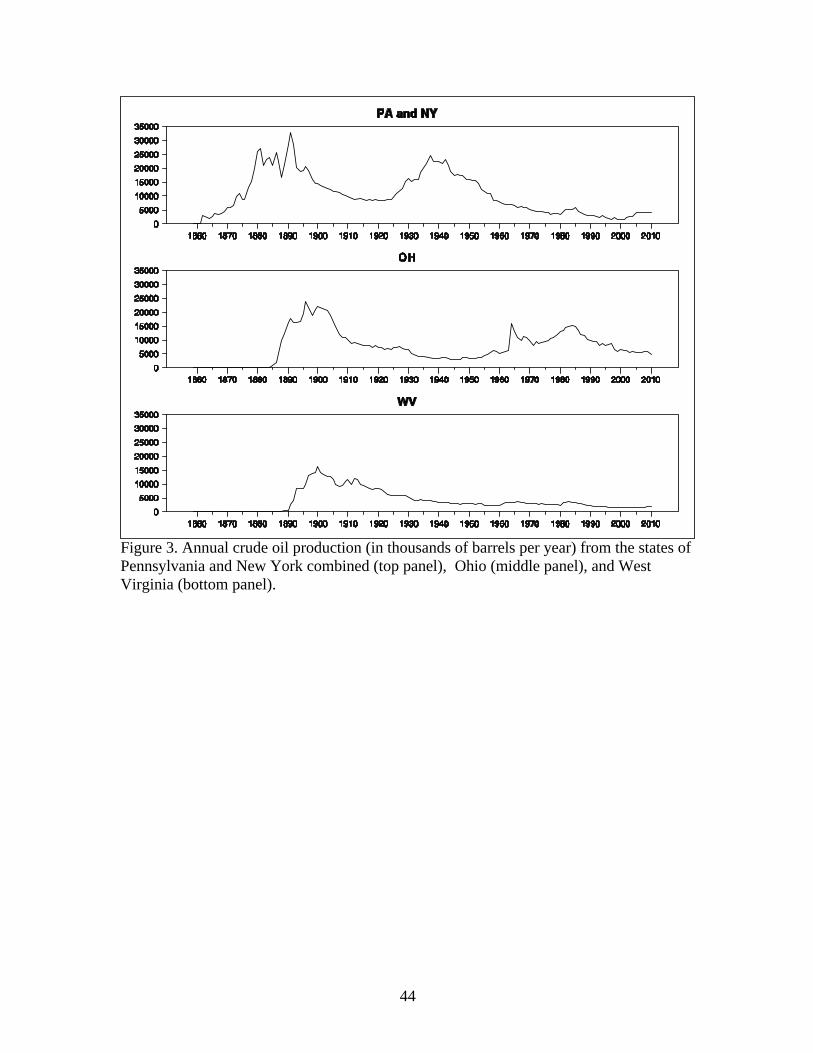
Although Pennsylvania was the most important source of U.S. oil production in the

19th century, the nation’s oil production continued to increase even after Pennsylvanian

production peaked in 1891. The reason is that later in the century, new sources of oil were

also being obtained from neighboring West Virginia and Ohio (see Figure 3). Production

from these two states was rising rapidly even as production from Pennsylvania and New

York started to fall. Ohio production would continue to rise before peaking in 1896, and

West Virginia did not peak until 1900.

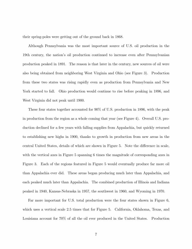
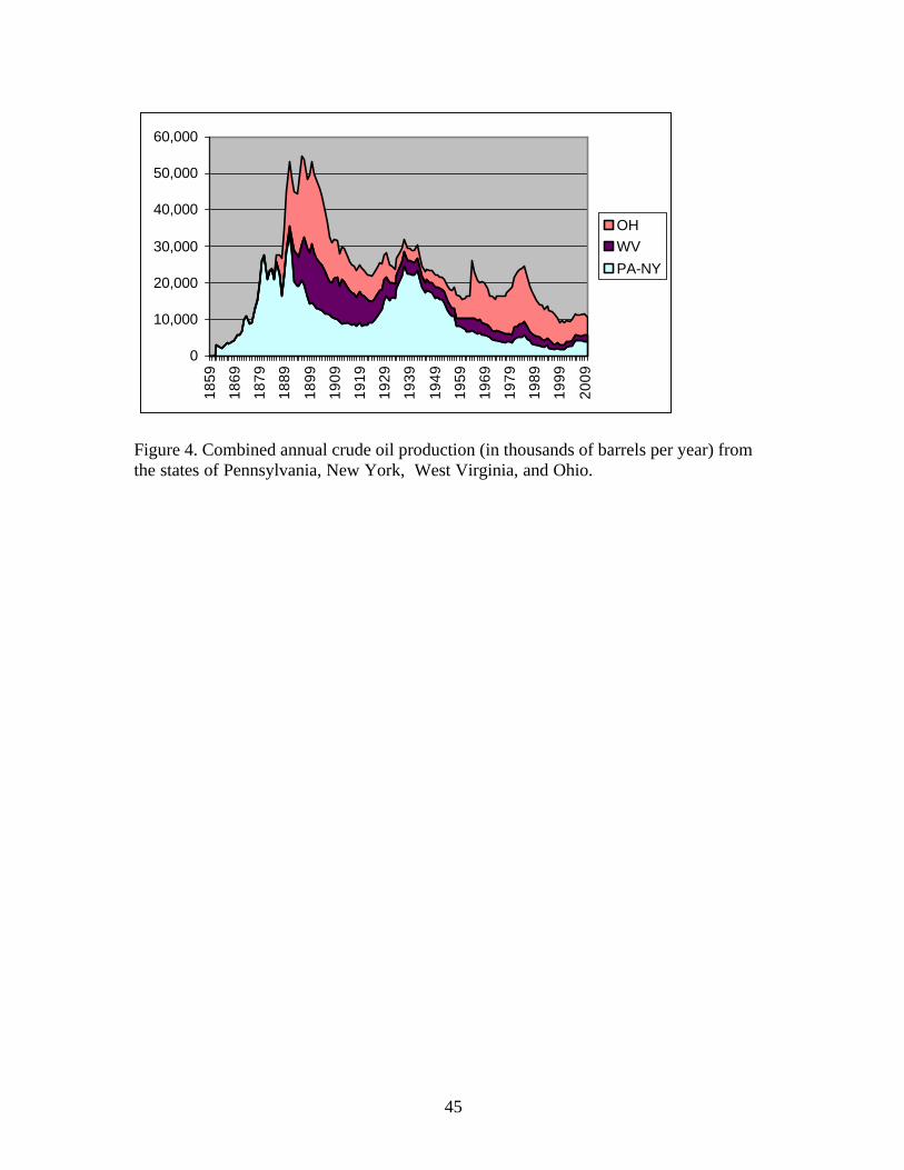
These four states together accounted for 90% of U.S. production in 1896, with the peak

in production from the region as a whole coming that year (see Figure 4). Overall U.S. pro-

duction declined for a few years with falling supplies from Appalachia, but quickly returned

to establishing new highs in 1900, thanks to growth in production from new areas in the

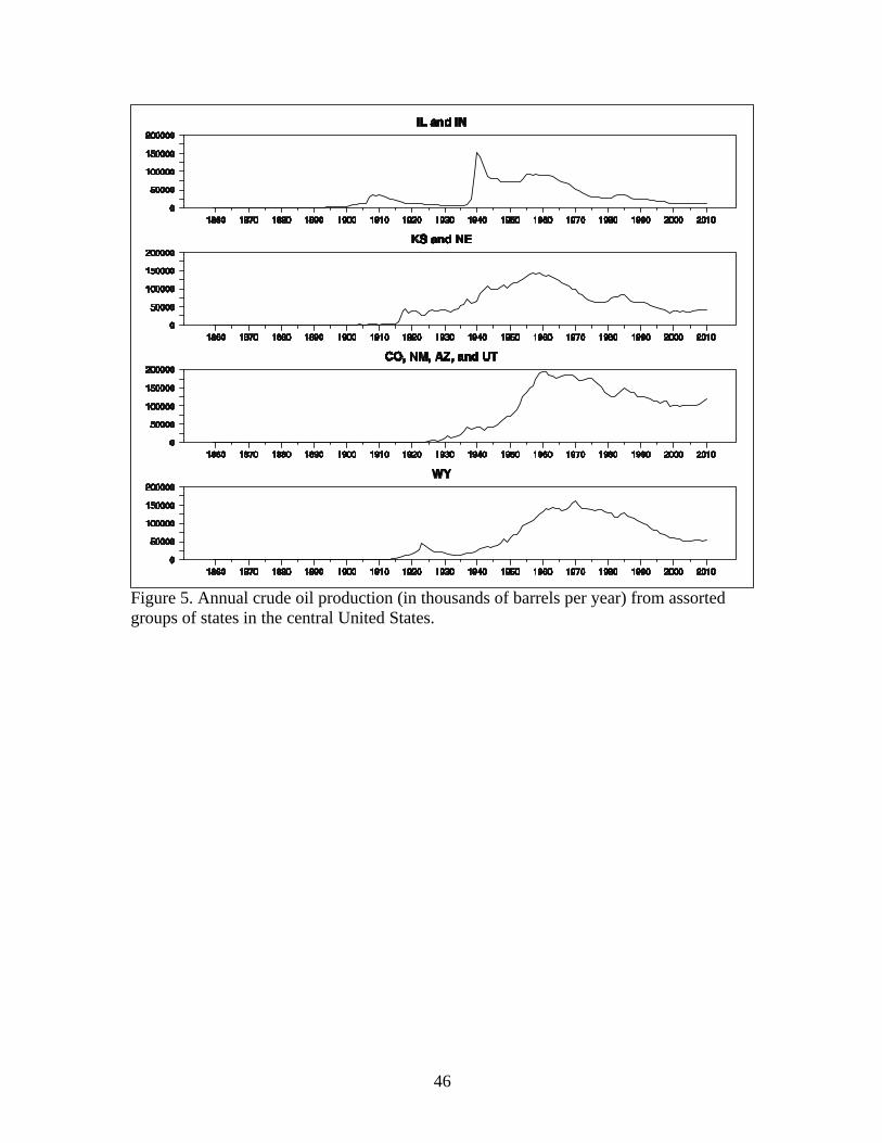
central United States, details of which are shown in Figure 5. Note the difference in scale,

with the vertical axes in Figure 5 spanning 6 times the magnitude of corresponding axes in

Figure 3. Each of the regions featured in Figure 5 would eventually produce far more oil

than Appalachia ever did. These areas began producing much later than Appalachia, and

each peaked much later than Appalachia. The combined production of Illinois and Indiana

peaked in 1940, Kansas-Nebraska in 1957, the southwest in 1960, and Wyoming in 1970.

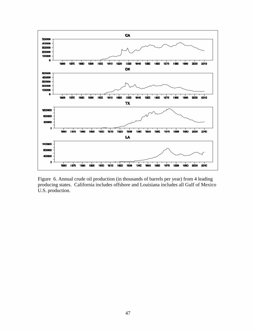
Far more important for U.S. total production were the four states shown in Figure 6,

which uses a vertical scale 2.5 times that for Figure 5. California, Oklahoma, Texas, and

Louisiana account for 70% of all the oil ever produced in the United States. Production

7

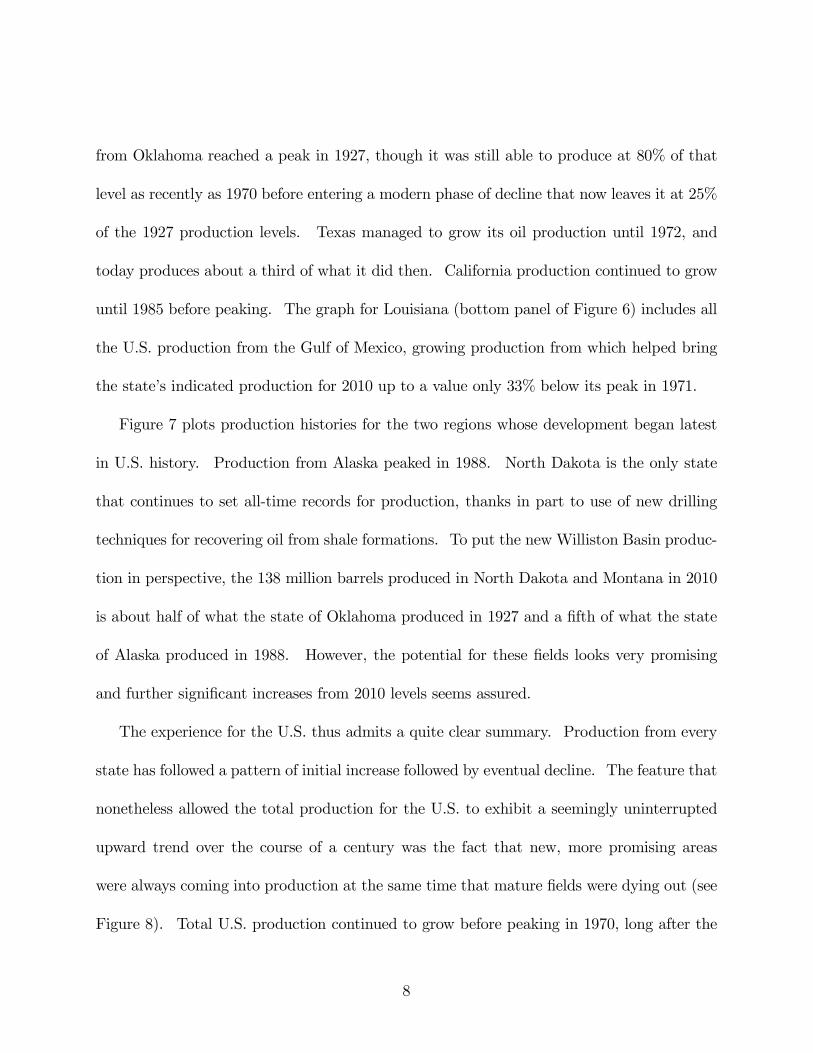
from Oklahoma reached a peak in 1927, though it was still able to produce at 80% of that

level as recently as 1970 before entering a modern phase of decline that now leaves it at 25%

of the 1927 production levels. Texas managed to grow its oil production until 1972, and

today produces about a third of what it did then. California production continued to grow

until 1985 before peaking. The graph for Louisiana (bottom panel of Figure 6) includes all

the U.S. production from the Gulf of Mexico, growing production from which helped bring

the state’s indicated production for 2010 up to a value only 33% below its peak in 1971.

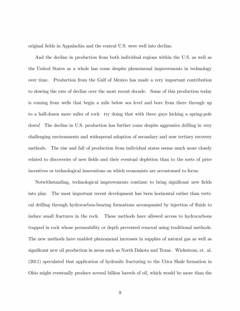
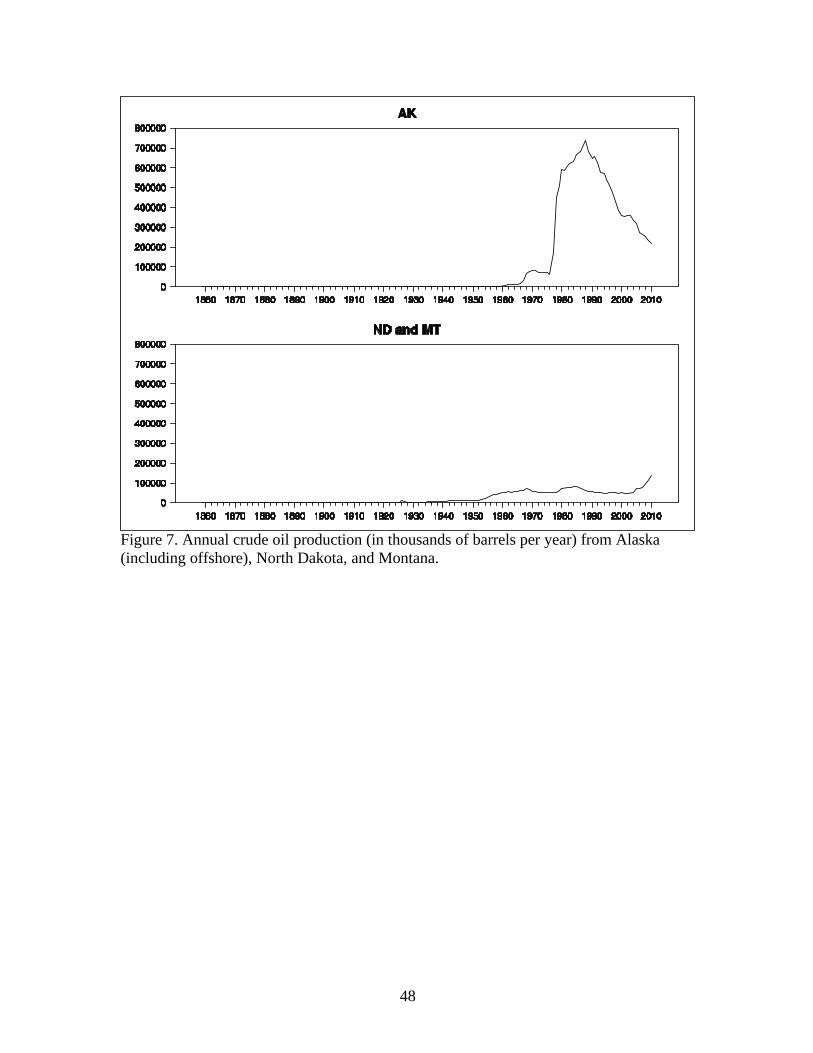
Figure 7 plots production histories for the two regions whose development began latest

in U.S. history. Production from Alaska peaked in 1988. North Dakota is the only state

that continues to set all-time records for production, thanks in part to use of new drilling

techniques for recovering oil from shale formations. To put the new Williston Basin produc-

tion in perspective, the 138 million barrels produced in North Dakota and Montana in 2010

is about half of what the state of Oklahoma produced in 1927 and a fifth of what the state

of Alaska produced in 1988. However, the potential for these fields looks very promising

and further significant increases from 2010 levels seems assured.

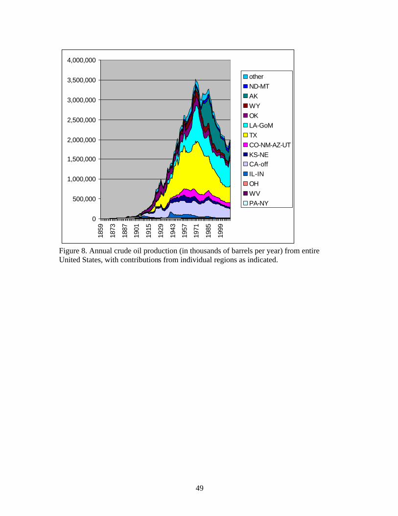
The experience for the U.S. thus admits a quite clear summary. Production from every

state has followed a pattern of initial increase followed by eventual decline. The feature that

nonetheless allowed the total production for the U.S. to exhibit a seemingly uninterrupted

upward trend over the course of a century was the fact that new, more promising areas

were always coming into production at the same time that mature fields were dying out (see

Figure 8). Total U.S. production continued to grow before peaking in 1970, long after the

8

original fields in Appalachia and the central U.S. were well into decline.

And the decline in production from both individual regions within the U.S. as well as

the United States as a whole has come despite phenomenal improvements in technology

over time. Production from the Gulf of Mexico has made a very important contribution

to slowing the rate of decline over the most recent decade. Some of this production today

is coming from wells that begin a mile below sea level and bore from there through up

to a half-dozen more miles of rock— try doing that with three guys kicking a spring-pole

down! The decline in U.S. production has further come despite aggressive drilling in very

challenging environments and widespread adoption of secondary and now tertiary recovery

methods. The rise and fall of production from individual states seems much more closely

related to discoveries of new fields and their eventual depletion than to the sorts of price

incentives or technological innovations on which economists are accustomed to focus.

Notwithstanding, technological improvements continue to bring significant new fields

into play. The most important recent development has been horizontal rather than verti-

cal drilling through hydrocarbon-bearing formations accompanied by injection of fluids to

induce small fractures in the rock. These methods have allowed access to hydrocarbons

trapped in rock whose permeability or depth prevented removal using traditional methods.

The new methods have enabled phenomenal increases in supplies of natural gas as well as

significant new oil production in areas such as North Dakota and Texas. Wickstrom, et. al.

(2011) speculated that application of hydraulic fracturing to the Utica Shale formation in

Ohio might eventually produce several billion barrels of oil, which would be more than the

9

cumulative production from the state up to this point. If that indeed turns out to be the

case, it could lead to a third peak in the graphs in Figure 3 for the Appalachian region that

exceeds either of the first two, though for comparison the projected lifetime output from

Utica would still only correspond to a few years of production from Texas at that state’s

peak.

Obviously price incentives and technological innovations matter a great deal. More oil

will be brought to the surface at a price of $100 a barrel than at $10 a barrel, and more

oil can be produced with the new technology than with the old. But it seems a mistake

to overstate the operative elasticities. By 1960, the real price of oil had fallen to a level

that was 1/3 its value in 1900. Over the same period, U.S. production of crude oil grew

to become 55 times what it had been in 1900. On the other hand, the real price of oil

rose 8-fold from 1970 to 2010, while U.S. production of oil fell by 43% over those same 40

years. The increase in production from 1900 to 1960 thus could in no way be attributed

to the response to price incentives. Likewise, neither huge price incentives nor impressive

technological improvements were sufficient to prevent the decline in production from 1970 to

2010. Further exploitation of offshore or deep shale resources may help put U.S. production

back on an upward trend for the next decade, but it seems unlikely ever again to reach the

levels seen in 1970.

10

1.2 World oil production, 1973-2010.

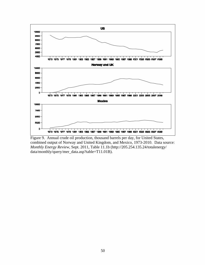
Despite the peak in U.S. production in 1970, world oil production was to grow to a level in

2010 that is 60% higher than it had been in 1970. The mechanics of this growth are the same

as allowed total U.S. production to continue to increase long after production from the initial

areas entered into decline— increases from new fields in other countries more than offset the

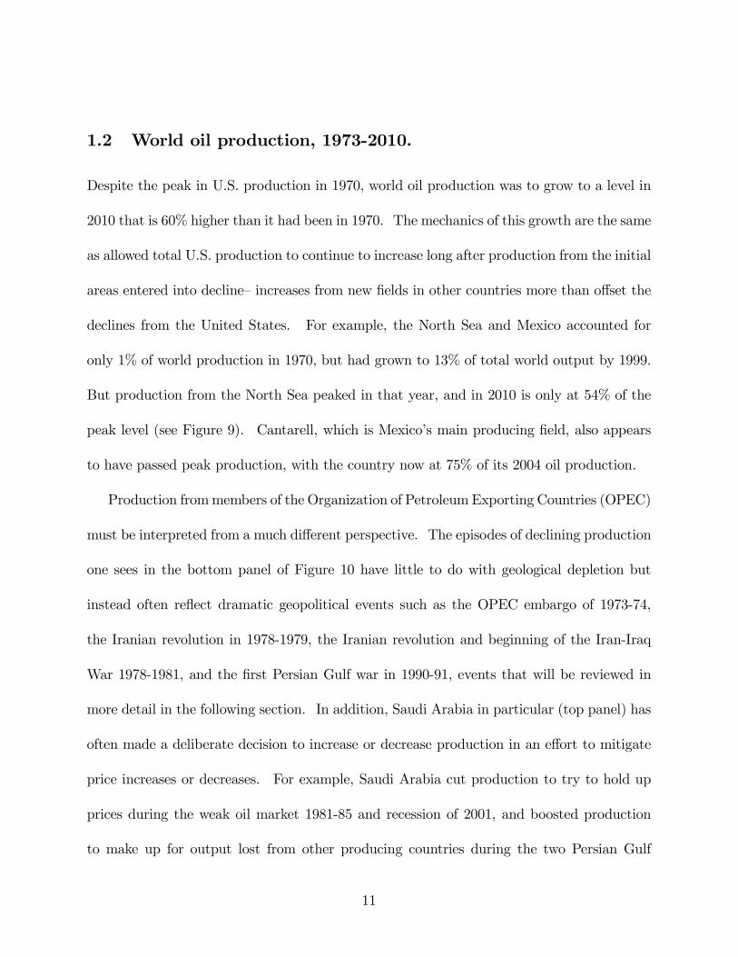
declines from the United States. For example, the North Sea and Mexico accounted for

only 1% of world production in 1970, but had grown to 13% of total world output by 1999.

But production from the North Sea peaked in that year, and in 2010 is only at 54% of the

peak level (see Figure 9). Cantarell, which is Mexico’s main producing field, also appears

to have passed peak production, with the country now at 75% of its 2004 oil production.

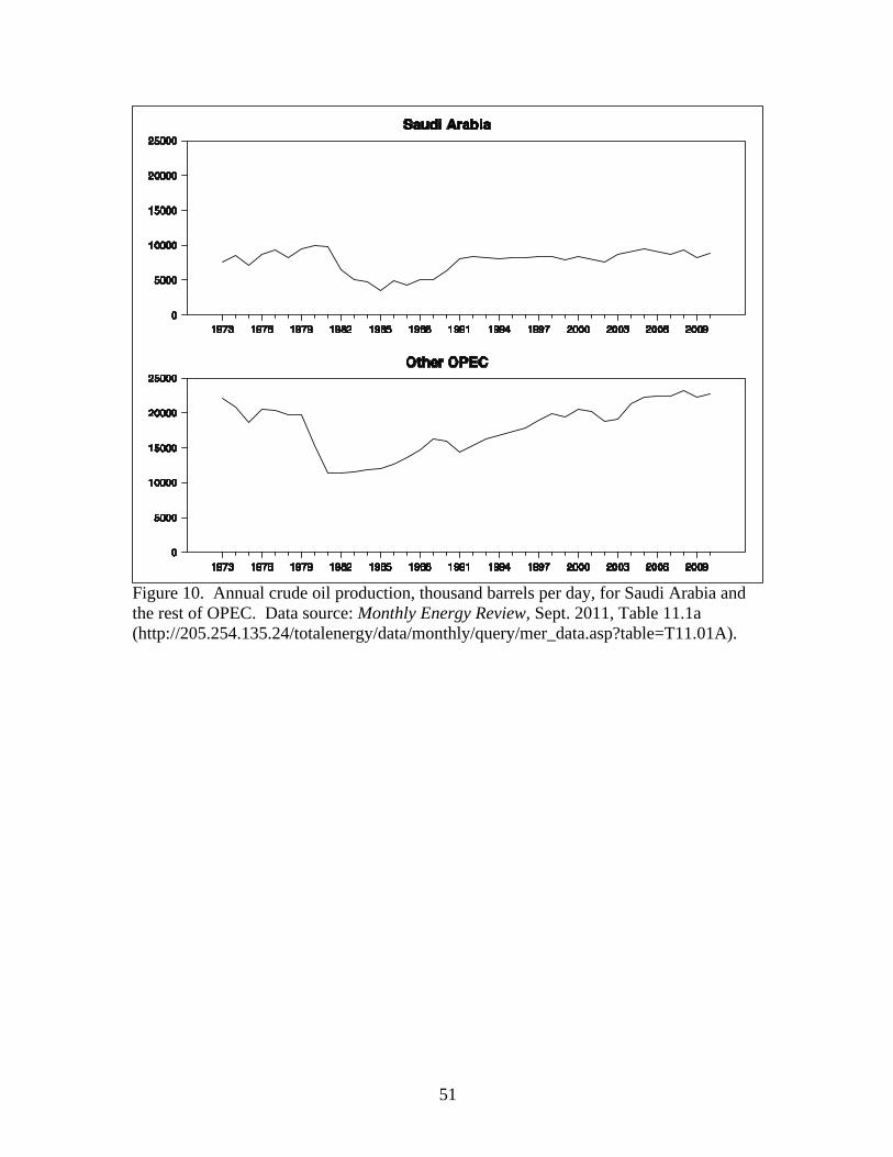
Production frommembers of the Organization of PetroleumExporting Countries (OPEC)

must be interpreted from a much different perspective. The episodes of declining production

one sees in the bottom panel of Figure 10 have little to do with geological depletion but

instead often reflect dramatic geopolitical events such as the OPEC embargo of 1973-74,

the Iranian revolution in 1978-1979, the Iranian revolution and beginning of the Iran-Iraq

War 1978-1981, and the first Persian Gulf war in 1990-91, events that will be reviewed in

more detail in the following section. In addition, Saudi Arabia in particular (top panel) has

often made a deliberate decision to increase or decrease production in an effort to mitigate

price increases or decreases. For example, Saudi Arabia cut production to try to hold up

prices during the weak oil market 1981-85 and recession of 2001, and boosted production

to make up for output lost from other producing countries during the two Persian Gulf

11

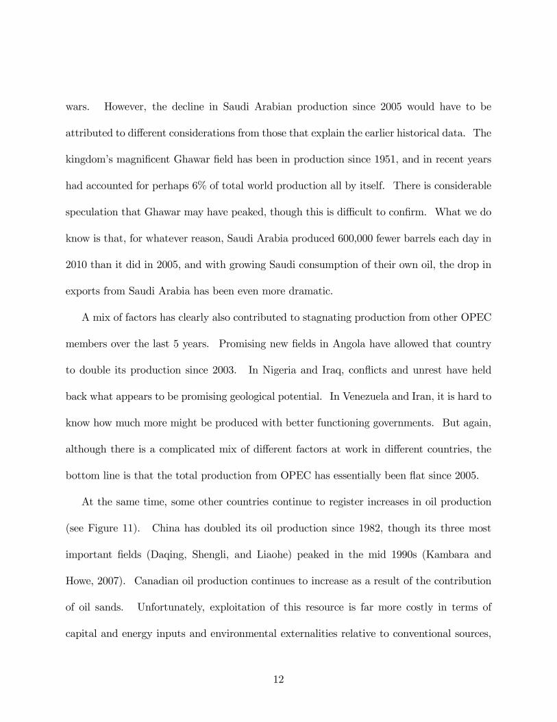
wars. However, the decline in Saudi Arabian production since 2005 would have to be

attributed to different considerations from those that explain the earlier historical data. The

kingdom’s magnificent Ghawar field has been in production since 1951, and in recent years

had accounted for perhaps 6% of total world production all by itself. There is considerable

speculation that Ghawar may have peaked, though this is difficult to confirm. What we do

know is that, for whatever reason, Saudi Arabia produced 600,000 fewer barrels each day in

2010 than it did in 2005, and with growing Saudi consumption of their own oil, the drop in

exports from Saudi Arabia has been even more dramatic.

A mix of factors has clearly also contributed to stagnating production from other OPEC

members over the last 5 years. Promising new fields in Angola have allowed that country

to double its production since 2003. In Nigeria and Iraq, conflicts and unrest have held

back what appears to be promising geological potential. In Venezuela and Iran, it is hard to

know how much more might be produced with better functioning governments. But again,

although there is a complicated mix of different factors at work in different countries, the

bottom line is that the total production from OPEC has essentially been flat since 2005.

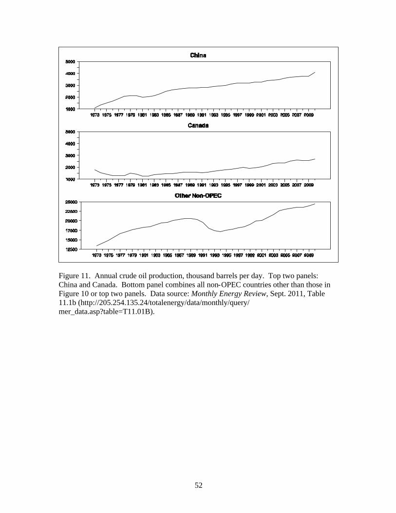
At the same time, some other countries continue to register increases in oil production

(see Figure 11). China has doubled its oil production since 1982, though its three most

important fields (Daqing, Shengli, and Liaohe) peaked in the mid 1990s (Kambara and

Howe, 2007). Canadian oil production continues to increase as a result of the contribution

of oil sands. Unfortunately, exploitation of this resource is far more costly in terms of

capital and energy inputs and environmental externalities relative to conventional sources,

12

and it is difficult to see it ever accounting for a major fraction of total world oil production.

Other regions such as Brazil, central Asia, and Africa have also seen significant gains in oil

production (bottom panel of Figure 11). Overall, global production of oil from all sources

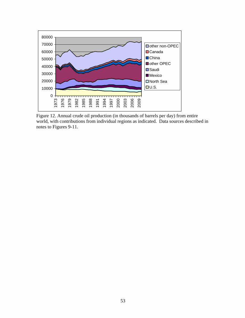
was essentially constant from 2005 to 2010 (see Figure 12).

1.3 Reconciling historical experience with the theory of exhaustible

resources.

The evidence from the preceding subsections can be summarized as follows. When one looks

at individual oil-producing regions, one does not see a pattern of continuing increases as a

result of ongoing technological progress. Instead there has inevitably been an initial gain as

key new fields were developed followed by subsequent decline. Technological progress and

the incentives of higher prices can temporarily reverse that decline, as was seen for example

in the impressive resurgence of Pennsylvanian production in the 1920s. In recent years these

same factors have allowed U.S. production to grow rather than decline, and that trend in the

U.S. may continue for some time. However, these factors have historically appeared to be

distinctly secondary to the broad reality that after a certain period of exploitation, annual

flow rates of production from a given area are going to start to decline. Those encouraged

by the 10% increase in U.S. oil production between 2008 and 2010 should remember that

the level of U.S. production in 2010 is still 25% below where it had been in 1990 (when the

real price of oil was half of what it is today) and 43% below the level of 1970 (when the real

price of oil was 1/8 of what it is today).

13

Some may argue that the peaking of production from individual areas is governed by quite

different economic considerations than would apply to the final peaking of total production

from all world sources combined. Certainly in an environment in which the market is pricing

oil as an essentially inexhaustible resource, the pattern of peaking documented extensively

above is perfectly understandable, given that so far there have always been enough new

fields somewhere in the world to take the place of declining production from mature regions.

One could also reason that, even if the price of oil has historically been following some

kind of Hotelling path, fields with different marginal extraction costs would logically be

developed at different times. Smith (2011) further noted that, according to the Hotelling

model, the date at which global production peaks would be determined endogenously by

the cumulative amount that could eventually be extracted and the projected time path

for the demand function. His analysis suggests that the date for an eventual peak in

global oil production should be determined by these economic considerations rather than

the engineering mechanics that have produced the historical record for individual regions

detailed above.

However, my reading of the historical evidence is as follows. (1) For much of the history

of the industry, oil has been priced essentially as if it were an inexhaustible resource. (2)

Although technological progress and enhanced recovery techniques can temporarily boost

production flows from mature fields, it is not reasonable to view these factors as the primary

determinants of annual production rates from a given field. (3) The historical source of

increasing global oil production is exploitation of new geographical areas, a process whose

14

promise at the global level is obviously limited. The combined implication of these three

observations is that, at some point there will need to be a shift in how the price of oil is

determined, with considerations of resource exhaustion playing a bigger role than they have

historically.

A factor accelerating the date of that transition is the phenomenal growth of demand for

oil from the emerging economies. Eight emerging economies— Brazil, China, Hong Kong,

India, Singapore, South Korea, Taiwan, and Thailand— accounted for 43% of the increase in

world petroleum consumption between 1998 and 2005 and for 135% of the increase between

2005 and 2010 (the rest of the world decreased its petroleum consumption over the latter

period in response to the big increase in price). 3 And, as Hamilton (2009a) noted, one could

easily imagine the growth in demand from the emerging economies continuing. One has

only to compare China’s one passenger vehicle per 30 residents today with the one vehicle

per 1.3 residents seen in the United States, or China’s 2010 annual petroleum consumption

of 2.5 barrels per person with Mexico’s 6.7 or the United States’ 22.4. Even if the world sees

phenomenal success in finding new sources of oil over the next decade, it could prove quite

challenging to keep up with both depletion from mature fields and rapid growth in demand

from the emerging economies, another reason to conclude that the era in which petroleum

is regarded as an essentially unlimited resource has now ended.

Some might infer that the decrease in Saudi Arabian production since 2005 reflects not

an inability to maintain production flows from the mature Ghawar field but instead is a

deliberate response to recognition of a growing importance of the scarcity rent. For example,

15

Hamilton (2009a) noted the following story on April 13, 2008 from Reuters news service:

Saudi Arabia’s King Abdullah said he had ordered some new oil discoveries left

untapped to preserve oil wealth in the world’s top exporter for future generations,

the official Saudi Press Agency (SPA) reported.

“I keep no secret from you that when there were some new finds, I told them,

‘no, leave it in the ground, with grace from God, our children need it’,” King

Abdullah said in remarks made late on Saturday, SPA said.

If that is indeed the interpretation, it is curious that we would see the private optimizing

choices predicted by Hotelling manifest by sovereign governments rather than the fields under

control of private oil companies. In any case, it must be acknowledged that calculation of

the correct Hotelling price is almost insurmountably difficult. It is hard enough for the best

forecasters accurately to predict supply and demand for the coming year. But the critical

calculation required by Hotelling is to evaluate the transversality condition that the resource

be exhausted when the price reaches that of a backstop technology or alternatively over the

infinite time horizon if no such backstop exists. That calculation is orders of magnitudes

more difficult than the seemingly simpler task of just predicting next year’s supply and

demand.

One could argue that the combined decisions of the many participants in world oil markets

can make a better determination of what the answer to the above calculation should be than

can any individual, meaning that if the current price seems inconsistent with a scenario

in which global oil production will soon reach a peak, then such a scenario is perhaps not

16

the most likely outcome. But saying that the implicit judgment from the market is the

best guess available is not the same thing as saying that this guess is going to prove to be

correct. The historical record surely dictates that we take seriously the possibility that

the world could soon reach a point from which a continuous decline in the annual flow rate

of production could not be avoided, and inquire whether the transition to a pricing path

consistent with that reality could prove to be a fairly jarring event. For this reason, it seems

worthwhile to review the historical record on the economic response to previous episodes in

which the price or supply of oil changed dramatically, to which we now turn in the next

section.

2 Oil prices and economic growth.

2.1 Historical oil price shocks.

There have been a number of episodes over the last half century in which conflicts in the

Middle East have led to significant disruptions in production of crude oil. These include

closure of the Suez Canal following the conflict between Egypt, Israel, Britain, and France

in October 1956, the oil embargo implemented by the Arab members of OPEC following the

Arab-Israeli War in October 1973, the Iranian revolution beginning in November 1978, the

Iran-Iraq War beginning in September of 1980, and the first Persian Gulf war beginning in

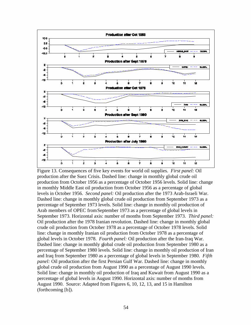
August 1990. Figure 13 summarizes the consequences of these 5 events for world oil supplies.

In each panel, the solid line displays the drop in production from the affected areas expressed

17

as a percentage of total world production prior to the crisis. In each episode, there were

some offsetting increases in production elsewhere in the world. The dashed lines in Figure

13 indicate the magnitude of the actual decline in total global production following each

event, again expressed as a fraction of world production. Each of these 5 episodes was

followed by a decrease in world oil production of 4-9%.

There have also been some other more minor supply disruptions over this period. These

include the combined effects of the second Persian Gulf war and strikes in Venezuela be-

ginning in December 2002, and the Libyan revolution in February 2011. The disruption in

supply associated with either of these episodes was about 2% of total global production at

the time, or less than a third the size of the average event in Figure 13.

There are other episodes since World War II when the price of oil rose abruptly in the

absence of a significant physical disruption in the supply of oil. Most notable of these would

be the broad upswing in the price of oil beginning in 2004, which accelerated sharply in

2007. The principal cause of this oil spike appears to have been strong demand for oil from

the emerging economies confronting the stagnating global production levels documented in

the previous sections (see Kilian, 2008, 2009, Hamilton, 2009b and Kilian and Hicks, 2011).

Less dramatic price increases followed the economic recovery from the East Asian Crisis

in 1997, dislocations associated with post World War II growth in 1947, and the Korean

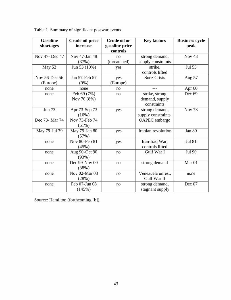
conflict in 1952-53. Table 1 summarizes a series of historical episodes discussed in Hamilton

(forthcoming). It is interesting that of the 11 episodes listed, 10 of these were followed by

a recession in the United States. The recession of 1960 is the only U.S. postwar recession

18

that was not preceded by a spike in the price of crude oil.

A large empirical literature has investigated the connection between oil prices and real

economic growth. Early studies documenting a statistically significant negative correlation

include Rasche and Tatom (1977, 1981) and Santini (1985). Empirical analysis of dynamic

forecasting regressions found that oil price changes could help improve forecasts of U.S. real

output growth (Hamilton, 1983; Burbidge and Harrison, 1984; Gisser and Goodwin, 1986).

However, these specifications, which were based on linear relations between the log change in

oil prices and the log of real output growth, broke down when the dramatic oil price decreases

of the mid-1980s were not followed by an economic boom. On the contrary, the mid-1980s

appeared to be associated with recession conditions in the oil-producing states (Hamilton

and Owyang, forthcoming). Mork (1989) found a much better fit to a model that allowed for

oil price decreases to have a different effect on the economy from oil price increases, though

Hooker (1996) demonstrated that this modification still had trouble describing subsequent

data. Other papers finding a significant connection between oil price increases and poor

economic performance include Santini (1992, 1994), Rotemberg andWoodford (1996), Daniel

(1997), and Carruth, Hooker and Oswald (1998).

Alternative nonlinear dynamic relations seem to have a significantly better fit to U.S. data

than Mork’s simple asymmetric formulation. Loungani (1986) and Davis (1987a, 1987b)

found that oil price decreases could actually reduce economic growth, consistent with the

claim that sectorial reallocations could be an important part of the economic transmission

mechanism resulting from changes in oil prices in either direction. Ferderer (1996), Elder

19

and Serletis (2010), and Jo (2011) showed that an increase in oil price volatility itself tends

to predict slower GDP growth, while Lee, Ni, and Ratti (1995) found that oil price increases

seem to affect the economy less if they occur following an episode of high volatility. Hamilton

(2003) estimated a flexible nonlinear form and found evidence for a threshold effect, in which

an oil price increase that simply reverses a previous decrease seems to have little effect on

the economy. Hamilton (1996), Raymond and Rich (1997), Davis and Haltiwanger (2001)

and Balke, Brown and Yücel (2002) produced evidence in support of related specifications,

while Carlton (2010) and Ravazzolo and Rothman (2010) reported that the Hamilton (2003)

specification performed well in an out-of-sample forecasting exercise using data as it would

have been available in real time. Kilian and Vigfusson (2011 [a]) found weaker (though

still statistically significant) evidence of nonlinearity than reported by other researchers.

Hamilton (2011) attributed their weaker evidence to use of a shorter data set and changes

in specification from other researchers.

A negative effect of oil prices on real output has also been reported for a number of other

countries, particularly when nonlinear functional forms have been employed. Mork, Olsen

and Mysen (1994) found that oil price increases were followed by reductions in real GDP

growth in 6 of the 7 OECD countries investigated, the one exception being the oil exporter

Norway. Cuñado and Pérez de Gracia (2003) found a negative correlation between oil prices

changes and industrial production growth rates in 13 out of 14 European economies, with

a nonlinear function of oil prices making a statistically significant contribution to forecast

growth rates for 11 of these. Jiménez-Rodríguez and Sánchez (2005) found a statistically

20

significant negative nonlinear relation between oil prices and real GDP growth in the U.S.,

Canada, Euro area overall, and 5 out of 6 European countries, though not in Norway or

Japan. Kim (2012) found a nonlinear relation in a panel of 6 countries, while Engemann,

Kliesen, and Owyang (2011) found that oil prices helped predict economic recessions in most

of the countries they investigated. Daniel, et. al. (2011) also found supporting evidence

in most of the 11 countries they studied. By contrast, Rasmussen and Roitman (2011)

found much less evidence for economic effects of oil shocks in an analysis of 144 countries.

However, their use of this larger sample of countries required using annual rather than the

monthly or quarterly data used in the other research cited above. Insofar as the effects

are high frequency and cyclical, they may be less apparent in annual average data. Kilian

(2009) has argued that the source of the oil price increase is also important, with increases

that result from strong global demand appearing to have more benign implications for U.S.

real GDP growth than oil price increases that result from shortages of supply.

Blanchard and Galí (2010) found evidence that the effects of oil shocks on the economy

have decreased over time, which they attributed to the absence of other adverse shocks that

had historically coincided with some big oil price movements, a falling value of the share

of oil in total expenses, more flexible labor markets, and better management of monetary

policy. Baumeister and Peersman (2011) also found that an oil price increase of a given

size seems to have a decreasing effect over time, but noted that the declining price-elasticity

of demand meant that a given physical disruption had a bigger effect on price and turned

out to have a similar effect on output as in the earlier data. Ramey and Vine (2010)

21

attributed the declining coefficients relating real GDP growth to oil prices to the fact that

the oil shocks of the 1970s were accompanied by rationing, which would have magnified the

economic dislocations. Ramey and Vine found that once they correct for this, the economic

effects have been fairly stable over time.

2.2 Interpreting the historical evidence.

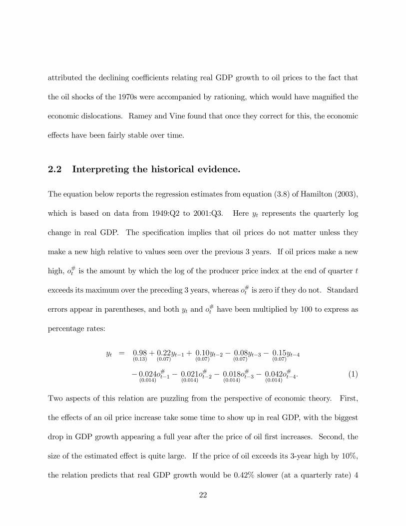
The equation below reports the regression estimates from equation (3.8) of Hamilton (2003),

which is based on data from 1949:Q2 to 2001:Q3. Here yt represents the quarterly log

change in real GDP. The specification implies that oil prices do not matter unless they

make a new high relative to values seen over the previous 3 years. If oil prices make a new

high, o#t is the amount by which the log of the producer price index at the end of quarter t

exceeds its maximum over the preceding 3 years, whereas o#t is zero if they do not. Standard

errors appear in parentheses, and both yt and o#t have been multiplied by 100 to express as

percentage rates:

yt = 0.98(0.13)

+ 0.22(0.07)

yt−1 + 0.10(0.07)

yt−2 − 0.08(0.07)

yt−3 − 0.15(0.07)

yt−4

− 0.024(0.014)

o#t−1 − 0.021(0.014)

o#t−2 − 0.018(0.014)

o#t−3 − 0.042(0.014)

o#t−4. (1)

Two aspects of this relation are puzzling from the perspective of economic theory. First,

the effects of an oil price increase take some time to show up in real GDP, with the biggest

drop in GDP growth appearing a full year after the price of oil first increases. Second, the

size of the estimated effect is quite large. If the price of oil exceeds its 3-year high by 10%,

the relation predicts that real GDP growth would be 0.42% slower (at a quarterly rate) 4

22

quarters later, with a modest additional decline coming from the dynamic implications of

o#t−4 for yt−1, yt−2, and yt−3.

To understand why effects of this magnitude are puzzling,4 suppose we thought of the

level of real GDP (Y ) as depending on capital K, labor N , and energy E according to the

production function,

Y = F (K,N,E).

Profit maximization suggests that the marginal product of energy should equal its relative

price, denoted PE/P :

∂F

∂E= PE/P.

Multiplying the above equation by E/F implies that the elasticity of output with respect to

energy use should be given by γ, the dollar value of expenditures on energy as a fraction of

GDP:

∂ lnF

∂ lnE=

PEE

PY= γ. (2)

Suppose we thought that wages adjust instantaneously to maintain full employment and that

changes in investment take much longer than a few quarters to make a significant difference

for the capital stock. Then neither K nor N would respond to a change in the real price of

energy, and

∂ lnY

∂ lnPE/P=

∂ lnF

∂ lnE

∂ lnE

∂ lnPE/P(3)

= γθ

for θ the price-elasticity of energy demand.

23

The energy expenditure share is a small number— the value of crude oil consumed by

the United States in 2010 corresponds to less than 4% of total GDP. Moreover, the short-

run price elasticity of demand θ is also very small (Dahl, 1993). Hence it seems that any

significant observed response to historical oil price increases could not be attributed to the

direct effects of decreased energy use on productivity, but instead would have to arise from

forces that lead to underemployment of labor and underutilization of capital. Such effects

are likely to operate from changes in the composition of demand rather than the physical

process of production itself.5 Unlike the above mechanism based on aggregate supply effects,

the demand effects could be most significant when the price-elasticity of demand is low.

For example, suppose that the demand for energy is completely inelastic in the short run,

so that consumers try to purchase the same physical quantity E of energy despite the energy

price increase. Then nominal saving or spending on other goods or services must decline

by E∆PE when the price of energy goes up. Letting C denote real consumption spending

and PC the price of consumption goods,

∂ lnC

∂ ln(PE/PC)=

PEE

PCC= γC

for γC the energy expenditure share in total consumption. Again, for the aggregate economy

γC is a modest number. Currently about 6% of total U.S. consumer spending is devoted to

energy goods and services6, though for the lower 60% of U.S. households by income, the share

is closer to 10% (Carroll, 2011). And although the increased spending on energy represents

income for someone else, it can take a considerable amount of time for oil company profits to

be translated into higher dividends for shareholders or increased investment expenditures.

24

Recycling the receipts of oil exporting countries on increased spending on U.S.-produced

goods and services can take even longer. These delays may be quite important in determining

the overall level of spending that governs short-run business cycle dynamics.

Edelstein and Kilian (2009) conducted an extensive investigation of U.S. monthly spend-

ing patterns over 1970 to 2006, looking at bivariate autoregressions of measures of consump-

tion spending on their own lags and on lags of energy prices. They scaled the energy price

measure so that a one unit increase would correspond to a 1% drop in total consumption

spending if consumers were to try to maintain real energy purchases at their original levels.

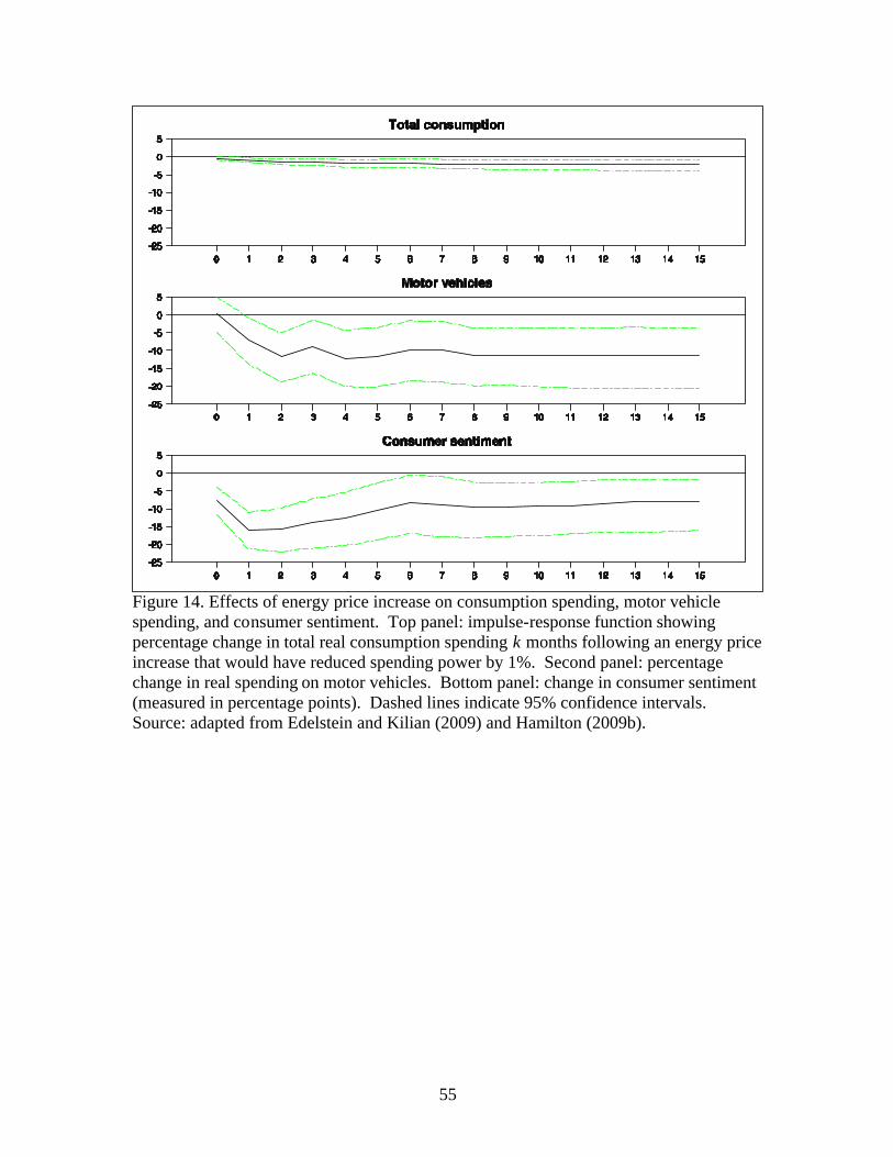
Figure 14 reproduces some of their key results. The top panel shows that, as expected,

an increase in energy prices is followed by a decrease in overall real consumption spending.

However, the same two puzzles mentioned in connection with (1) occur again here. First,

although consumers’ spending power first fell at date 0 on the graph, the decline in con-

sumption spending is not immediate but continues to increase in size up to a year after the

initial shock. Second, although the initial shock corresponded to an event that might have

forced a consumer to cut total spending by 1%, after 12 months, we see total spending down

2.2%.

The details of Edelstein’s and Kilian’s other analysis suggest some explanations for both

the dynamics and the apparent multiplier effects. The second panel in Figure 14 looks

at one particular component of consumption spending, namely spending on motor vehicles

and parts. Here the decline is essentially immediate, and quite large relative to normal

expenditures on this particular category. The drop in demand for domestically manufactured

25

motor vehicles could lead to idled capital and labor as a result of traditional Keynesian

frictions in adjusting wages and prices, and could be an explanation for both the multiplier

and the dynamics observed in the data. Hamilton (1988) showed that multiplier effects

could also arise in a strictly neoclassical model with perfectly flexible wages and prices. In

that model, the technological costs associated with trying to reallocate specialized labor

or capital could result in a temporary period of unemployment as laid-off workers wait for

demand for their sector to resume. Bresnahan and Ramey (1993), Hamilton (2009b), and

Ramey and Vine (2010) demonstrated the economic importance of shifts in motor vehicle

demand in the recessions that followed several historical oil shocks.

Another feature of the consumer response to an energy price increase uncovered by Edel-

stein and Kilian is a sharp and immediate drop in consumer sentiment (see the bottom panel

of Figure 14). Again, this could produce changes in spending patterns whose consequences

accumulate over time through Keynesian and other multiplier effects.

Bohi (1989) was among the early doubters of the thesis that oil prices were an important

contributing factor in postwar recessions, noting that the industries in which one sees the

biggest response were not those for which energy represented the biggest component of total

costs. However, subsequent analyses allowing for nonlinearities found effects for industries

for which energy costs were important both for their own production as well as for the

demand for their goods (Lee and Ni, 2002; Herrera, Lagalo and Wada, 2011).

Bernanke, Gertler and Watson (1997) suggested that another mechanism by which oil

price increases might have affected aggregate demand is through a contractionary response

26

of monetary policy. They presented simulations suggesting that , if the Federal Reserve had

kept interest rates from rising subsequent to historical oil shocks, most of the output decline

could have been avoided. However, Hamilton and Herrera (2004) demonstrated that this

conclusion resulted from the authors’ assumption that the effects of oil price shocks could

be captured by 7 monthly lags of oil prices, a specification that left out the biggest effects

found by earlier researchers. When the Bernanke, et. al. analysis is reproduced using 12

lags instead of 7, the conclusion from their exercise would be that even quite extraordinarily

expansionary monetary policy could not have eliminated the contractionary effects of an oil

price shock.

Hamilton (2009b) noted that what happened in the early stages of the 2007-2009 recession

was quite consistent with the pattern observed in the recessions that followed earlier oil

shocks. Spending on the larger domestically manufactured light vehicles plunged even as

sales of smaller imported cars went up. Had it not been for the lost production from

the domestic auto sector, U.S. real GDP would have grown 1.2% during the first year of

the recession. Historical regressions based on energy prices would have predicted much of

the falling consumer sentiment and slower consumer spending during the first year of the

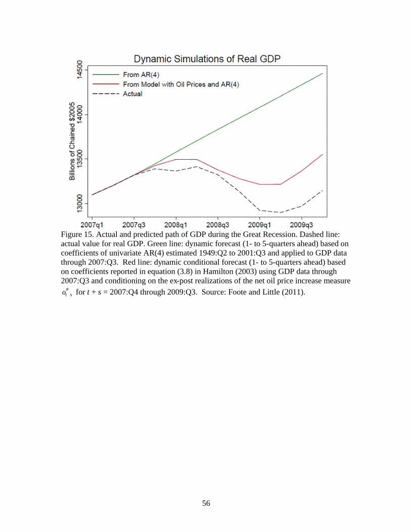
downturn. Figure 15 updates and extends a calculation from Hamilton (2009b), in which

the specific parameter values from the historically estimated regression (1) were used in

a dynamic simulation to predict what would have happened to real GDP over the period

2007:Q4 to 2009:Q3 based solely on the changes in oil prices. The pattern and much of the

magnitude of the initial downturn are consistent with the historical experience.

27

Of course, there is no question that the financial crisis in the fall of 2008 was a much more

significant event in turning what had been a modest slowdown up to that point into what

is now being referred to as the Great Recession. Even so, Hamilton (2009b) noted that the

magnitude of the problems with mortgage delinquencies could only have been aggravated by

the weaker economy, and suggested that the oil price spike of 2007-2008 should be counted

as an important factor contributing to the early stages of that recession as well as a number

of earlier episodes.

2.3 Implications for future economic growth and climate change.

The increases in world petroleum production over the first 150 years of the industry have

been quite impressive. But given the details behind that growth, it would be prudent

to acknowledge the possibility that world production could soon peak or enter a period of

rocky plateau. If we should enter such an era, what does the observed economic response

to past historical oil supply disruptions and price increases suggest could be in store for the

economy?

The above analysis suggests that historically the biggest economic effects have come from

cyclical factors that led to underutilization of labor and capital and drove output below the

level that would be associated with full employment. If we are asking about the character of

an alternative long-run growth path, most economists would be more comfortable assuming

that the economy would operate close to potential along the adjustment path. For purposes

of that question, the relatively small value for the energy expenditure share γ in equation

28

(2) would seem to suggest a modest elasticity of total output with respect to energy use and

relatively minor effects.

One detail worth noting, however, is that historically the energy share has changed

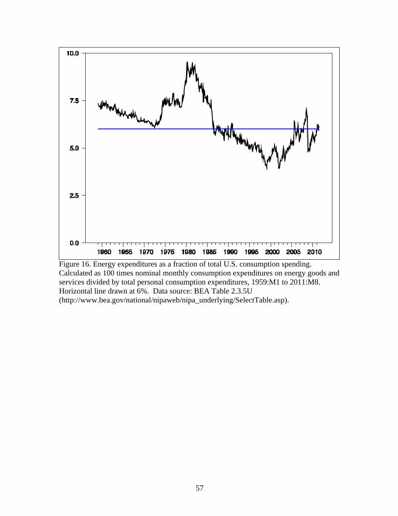
dramatically over time. Figure 16 plots the consumption expenditure share γC since 1959.

Precisely because demand is very price-inelastic in the short run, when the real price of

oil doubles, the share nearly does as well. The relatively low share in the late 1990s and

early 2000s, to which Blanchard and Galí (2010) attributed part of the apparent reduced

sensitivity of the economy to oil shocks, basically disappeared with the subsequent price

increases. If a peaking of global production does result in further big increases in the

price of oil, it is quite possible that the expenditure share would increase significantly from

where it is now, in which case even a frictionless neoclassical model would conclude that the

economic consequences of reduced energy use would have to be significant.

In addition to the response of supply to these price increases discussed in Section 1, an-

other key parameter is the long-run price-elasticity of demand. Here one might take comfort

from the observation that, given time, the adjustments of demand to the oil price increases of

the 1970s were significant. For example, U.S. petroleum consumption declined 17% between

1978 and 1985 at the same time that U.S. real GDP increased by 21%. However, Dargay

and Gately (2010) attributed much of this conservation to one-time effects, such as switching

away from using oil for electricity generation and space heating, that would be difficult to

repeat on an ongoing basis. Knittel (2011) was more optimistic, noting that there has been

ongoing technological improvement in engine and automobile design over time, with most

29

of this historically being devoted to making cars larger and more powerful rather than more

fuel-efficient. If the latter were to become everyone’s priority, significant reductions in oil

consumption might come from this source.

Knowing what the future will bring in terms of adaptation of both the supply and demand

for petroleum is inherently difficult. However, it is not nearly as hard to summarize the

past. Coping with a final peak in world oil production could look pretty similar to what

we observed as the economy adapted to the production plateau encountered over 2005-2009.

That experience appeared to have much in common with previous historical episodes that

resulted from temporary geopolitical conflict, being associated with significant declines in

employment and output. If the future decades look like the last 5 years, we are in for a

rough time.

Most economists view the economic growth of the last century and a half as being fueled

by ongoing technological progress. Without question, that progress has been most impres-

sive. But there may also have been an important component of luck in terms of finding

and exploiting a resource that was extremely valuable and useful but ultimately finite and

exhaustible. It is not clear how easy it will be to adapt to the end of that era of good

fortune.

Let me close with a few observations on the implications for climate change. Clearly

reduced consumption of petroleum by itself would mean lower greenhouse gas emissions.

Moreover, since GDP growth has historically been the single biggest factor influencing the

growth of emissions (Hamilton and Turton, 2002), the prospects for potentially rocky eco-

30

nomic growth explored above would be another factor slowing growth of emissions. But

the key question in terms of climate impact is what we might do instead, since many of

the alternative sources of transportation fuel have a significantly bigger carbon footprint

than those we relied on in the past. For example, creating a barrel of synthetic crude from

surface-mined Canadian oil sands may emit twice as much carbon dioxide equivalents as are

associated with producing a barrel of conventional crude, while in-situ processing of oil sands

could produce three times as much (Charpentier, Bergerson and MacLean, 2009). This is

not quite as alarming as it sounds, since greenhouse gas emissions associated with produc-

tion of the crude itself are still dwarfed by those released when the gasoline is combusted in

the end-use vehicle. The median study surveyed by Charpentier, Bergerson and MacLean

(2009) concluded that on a well-to-wheel basis, vehicles driven by gasoline produced from

surface-mined oil sands would emit 17% more grams of carbon dioxide equivalent per kilo-

meter driven compared to gasoline from conventional petroleum. Enhanced oil recovery

and conversion of natural gas to liquid fuels are also associated with higher greenhouse gas

emissions per kilometer driven than conventional petroleum, though these increases are more

modest than those for oil sands. On the other hand, creating liquid fuels from coal or oil

shale could increase well-to-wheel emissions by up to a factor of two (Brandt and Farrell,

2007).

In any case, if the question is whether the world should decrease combustion of gasoline

produced from conventional petroleum sources, we may not have any choice.

31

Notes

1See Fouquet and Pearson (2006, 2012) on the history of the cost of illumination.

2See for example Williamson and Daum (1959, pp. 44-48).

3Data source: Total petroleum consumption, EIA (http://www.eia.gov/cfapps/ipdbproject/

iedindex3.cfm?tid=5&pid=5&aid=2&cid=regions&syid=1980&eyid=2010&unit=TBPD)

4The discussion in this paragraph is adapted from Hamilton (forthcoming [a]).

5Other neoclassical models explore the possibility of asymmetric or multiplier effects

arising through utilization of capital (Finn, 2000) or putty-clay capital (Atkeson and Kehoe,

1999). Related general equilibrium investigations include Kim and Loungani (1992) and

Leduc and Sill (2004).

6See BEATable 2.3.5.u (http://www.bea.gov/national/nipaweb/nipa_underlying/SelectTable.asp).

32

ReferencesArrow, Kenneth J. and Sheldon Chang (1982), “Optimal Pricing, Use and Exploration of

Uncertain Natural Resource Stocks,” Journal of Environmental Economics and Management

9, pp. 1-10.

Atkeson, Andrew and Patrick J. Kehoe (1999), “Models of Energy Use: Putty-putty

Versus Putty-clay,” American Economic Review 89, pp. 1028-1043.

Balke, Nathan S., Stephen P.A. Brown, and Mine Yücel (2002), “Oil Price Shocks and

the U.S. Economy: Where Does the Asymmetry Originate?,” Energy Journal 23, pp. 27-52.

Baumeister, Christiane and Gert Peersman (2011), “Time-Varying Effects of Oil Supply

Shocks on the U.S. Economy”, working paper, Bank of Canada.

Bernanke, Ben S., Mark Gertler, and Mark Watson (1997), “Systematic Monetary Policy

and the Effects of Oil Price Shocks,” Brookings Papers on Economic Activity 1:1997, pp.

91-142.

Blanchard, Olivier J., and Jordi Galí (2010), “The Macroeconomic Effects of Oil Price

Shocks: Why are the 2000s so Different from the 1970s?” in Jordi Galí and Mark Gertler

(eds.), International Dimensions of Monetary Policy, pp. 373-428, University of Chicago

Press (Chicago, IL).

Bohi, Douglas R. (1989), Energy Price Shocks and Macroeconomic Performance, Wash-

ington D.C.: Resources for the Future.

Brandt, Adam R., and Alexander E. Farrell (2007), “Scraping the Bottom of the Bar-

rel: Greenhouse Gas Emission Consequences of a Transition to Low-Quality and Synthetic

33

Petroleum Resources,” Climatic Change 84, pp. 241-263.

Bresnahan, Timothy F. and Valerie A. Ramey (1993), “Segment Shifts and Capacity

Utilization in the U.S. Automobile Industry,” American Economic Review Papers and Pro-

ceedings 83, pp. 213-218.

Burbidge, John, and Alan Harrison (1984), “Testing for the Effects of Oil-Price Rises

Using Vector Autoregressions,” International Economic Review 25, pp. 459-484.

Carlton, Amelie Benear (2010), “Oil Prices and Real-time Output Frowth,” Working

paper, University of Houston.

Carroll, Daniel (2011), “The Cost of Food and Energy across Consumers,” Economic

Trends (March 14), Federal Reserve Bank of Cleveland (http://www.clevelandfed.org/research/

trends/2011/0411/01houcon.cfm).

Carruth, Alan A., Mark A. Hooker, and Andrew J. Oswald (1998), “Unemployment Equi-

libria and Input Prices: Theory and Evidence from the United States,” Review of Economics

and Statistics 80, pp. 621-628.

Charpentier, Alex D., Joule A Bergerson and Heather LMacLean (2009), “Understanding

the Canadian Oil Sands Industry’s Greenhouse Gas Emissions,” Environmental Research

Letters 4, pp. 1-11.

Cuñado, Juncal and Fernando Pérez de Gracia (2003), “Do Oil Price Shocks Matter?

Evidence for some European Countries,” Energy Economics 25, pp. 137—154.

Dahl, Carol A. (1993), “A Survey of Oil Demand Elasticities for Developing Countries,”

OPEC Review 17(Winter), pp. 399-419.

34

Daniel, Betty C. (1997), “International Interdependence of National Growth Rates: A

Structural Trends Analysis,” Journal of Monetary Economics 40, pp. 73-96.

_____, Christian M. Hafner, Hans Manner, and Léopold Simar (2011), “Asymmetries

in Business Cycles: The Role of Oil Production”, working paper, University of Albany.

Dargay, Joyce M. and Dermot Gately (2010), “World Oil Demand’s Shift toward Faster

Growing and Less Price-Responsive Products and Regions,” Energy Policy 38, pp. 6261-

6277.

Dasgupta, Partha, and Geoffrey Heal (1979), Economic Theory and Exhaustible Re-

sources, Cambridge: Cambridge University Press.

Davis, Steven J. (1987a), “Fluctuations in the Pace of Labor Reallocation,” in Karl

Brunner and Allan H. Meltzer (eds.), Empirical Studies of Velocity, Real Exchange Rates,

Unemployment and Productivity, Carnegie-Rochester Conference Series on Public Policy, 24,

Amsterdam: North Holland.

_____ (1987b), “Allocative Disturbances and Specific Capital in Real Business Cycle

Theories,” American Economic Review Papers and Proceedings 77, pp. 326-332.

_____ and John Haltiwanger (2001), “Sectoral Job Creation and Destruction Re-

sponses to Oil Price Changes,” Journal of Monetary Economics 48, pp. 465-512.

Derrick’s Hand-Book of Petroleum: A Complete Chronological and Statistical Review

of Petroleum Developments from 1859 to 1898 (1898), Oil City, PA: Derrick Publishing

Company, Obtained through Google Books.

Edelstein, Paul and Lutz Kilian (2009), “How Sensitive are Consumer Expenditures to

35

Retail Energy Prices?”, Journal of Monetary Economics 56, pp. 766-779.

Elder, John and Apostolos Serletis (2010), “Oil Price Uncertainty,” Journal of Money,

Credit and Banking 42, pp. 1138-1159

Engemann, Kristie M. Kevin L. Kliesen, and Michael T. Owyang (2011), “Do Oil Shocks

Drive Business Cycles? Some U.S. and International Evidence,” Macroeconomic Dynamics,

15 (S3), pp 498 - 517.

Ferderer, J. Peter (1996), “Oil Price Volatility and the Macroeconomy: A Solution to

the Asymmetry Puzzle,” Journal of Macroeconomics 18, pp. 1-16.

Finn, Mary G. (2000), “Perfect Competition and the Effects of Energy Price Increases

on Economic Activity,” Journal of Money, Credit and Banking 32, pp. 400-416.

Foote, Christopher L. and Jane S. Little (2011), “Oil and the Macroeconomy in a Chang-

ing World: A Conference Summary,” Public Policy Discussion Paper, Federal Reserve Bank

of Boston.

Fouquet, Roger and Peter J.G. Pearson (2006), “Seven Centuries of Energy Services:

The Price and Use of Light in the United Kingdom (1300-2000),” Energy Journal 27, pp.

139-177.

_____ and _____ (2012), “The Long Run Demand for Lighting: Elasticities and

Rebound Effects in Different Phases of Economic Development,” Economics of Energy and

Environmental Policy 1, pp. 1-18.

Gisser, Micha, and Thomas H. Goodwin (1986), “Crude Oil and the Macroeconomy:

Tests of Some Popular Notions,” Journal of Money, Credit, and Banking 18, pp. 95-103.

36

Hamilton, Clive, and Hal Turton (2002), “Determinants of Emissions Growth in OECD

Countries,” Energy Policy 30, pp. 63—71.

Hamilton, James D. (1983), “Oil and the Macroeconomy Since World War II,” Journal

of Political Economy 91, pp. 228-248.

_____ (1988), “A Neoclassical Model of Unemployment and the Business Cycle,”

Journal of Political Economy 96, pp. 593-617.

_____ (1996), “This is What Happened to the Oil Price Macroeconomy Relation,”

Journal of Monetary Economics 38, pp. 215-220.

_____ (2003), “What is an Oil Shock?”, Journal of Econometrics 113, pp. 363-398.

_____ (2009a), “Understanding Crude Oil Prices,” Energy Journal 30, pp. 179-206.

_____ (2009b), “Causes and Consequences of the Oil shock of 2007-08,” Brookings

Papers on Economic Activity Spring 2009, pp. 215-261.

_____ (2011), “Nonlinearities and the Macroeconomic Effects of Oil Prices,” Macro-

economic Dynamics, 15 (S3), pp 364 - 378

_____ (forthcoming), “Historical Oil Shocks,” Handbook of Major Events in Economic

History, edited by Randall Parker and Robert Whaples, Routledge.

_____, and Ana Maria Herrera (2004), “Oil Shocks and Aggregate Macroeconomic

Behavior: The Role of Monetary Policy,” Journal of Money, Credit, and Banking 36, pp.

265-286

_____, and Michael T. Owyang (forthcoming), “The Propagation of Regional Reces-

sions,” forthcoming, Review of Economics and Statistics.

37

Herrera, Ana María, Latika Gupta Lagalo and Tatsuma Wada (2011), “Oil Price Shocks

and Industrial Production: Is the Relationship Linear?,”Macroeconomic Dynamics, 15 (S3),

pp 472 - 497

Hooker, Mark A. (1996), “What Happened to the Oil Price-Macroeconomy Relation-

ship?”, Journal of Monetary Economics 38, pp. 195-213.

Hotelling, Harold (1931), “The Economics of Exhaustible Resources,” Journal of Political

Economy 39, pp. 137-75.

Jenkins, Gilbert (1985), Oil Economists’ Handbook, London: British Petroleum Com-

pany.

Jiménez-Rodríguez, Rebeca and Marcelo Sánchez (2005), “Oil Price Shocks and Real

GDP Growth: Empirical Evidence for some OECD Countries,” Applied Economics 37, pp.

201—228.

Jo, Soojin (2011), “The Effects of Oil Price Uncertainty on the Macroeconomy,” working

paper, UCSD.

Kambara, Tatsu and Christopher Howe (2007), China and the Global Energy Crisis,

Cheltenham, UK: Edward Elgar.

Kilian, Lutz (2008), ““The Economic Effects of Energy Price Shocks,” Journal of Eco-

nomic Literature 46, pp. 871-909.

_____ (2009), “Not All Oil Price Shocks Are Alike: Disentangling Demand and Supply

Shocks in the Crude Oil Market”, American Economic Review 99, pp. 1053-1069.

_____, and Bruce Hicks (2011), “Did Unexpectedly Strong Economic Growth Cause

38

the Oil Price Shock of 2003-2008?”, working paper, University of Michigan.

_____ and Robert J. Vigfusson (2011 [a]), “Are the Responses of the U.S. Economy

Asymmetric in Energy Price Increases and Decreases?”, Quantitative Economics, 2, pp.

419-453.

____ and _____ (2011 [b]), “Nonlinearities in the Oil-Output Relationship,”Macro-

economic Dynamics, 15 (S3), pp 337 - 363

Kim, Dong Heon (2012), “What is an Oil Shock? Panel Data Evidence,” Empirical

Economics, 43, pp. 121 - 143

Kim, In-Moo and Prakash Loungani (1992), “The Role of Energy in Real Business Cycle

Models,” Journal of Monetary Economics 29, pp. 173-189.

Knittel, Christopher R. (2011), “Automobiles on Steroids: Product Attribute Trade-offs

and Technological Progress in the Automobile Sector,” American Economic Review, 101,

pp. 3368-3399.

Krautkraemer, Jeffrey A. (1998), “Nonrenewable Resource Scarcity,” Journal of Eco-

nomic Literature 36, pp. 2065-2107.

Leduc, Sylvain and Keith Sill (2004), “A Quantitative Analysis of Oil-Price Shocks,

Systematic Monetary Policy, and Economic Downturns,” Journal of Monetary Economics

51, pp. 781-808.

Lee, Kiseok and Shawn Ni (2002), “On the Dynamic Effects of Oil Price Shocks: A Study

Using Industry Level Data,” Journal of Monetary Economics 49, pp. 823—852.

_____, _____, and Ronald A. Ratti (1995), “Oil Shocks and the Macroeconomy:

39

The Role of Price Variability,” Energy Journal 16, pp. 39-56.

Loungani, Prakash (1986), “Oil Price Shocks and the Dispersion Hypothesis,” Review of

Economics and Statistics 68, pp. 536-539.

Mork, Knut A. (1989), “Oil and the Macroeconomy When Prices Go Up and Down: An

Extension of Hamilton’s Results,” Journal of Political Economy 91, pp. 740-744.

_____, Øystein Olsen, and Hans Terje Mysen (1994), “Macroeconomic Responses to

Oil Price Increases and Decreases in Seven OECD Countries,” Energy Journal 15, no. 4, pp.

19-35.

Pindyck, Robert S. (1978), “The Optimal Exploration and Production of Nonrenewable

Resources,” Journal of Political Economy 86, pp. 841-861.

Ramey, Valerie A. and Daniel J. Vine (2010), “Oil, Automobiles, and the U.S. Economy:

How Much Have Things Really Changed? In D. Acemoglu and M. Woodford, eds., NBER

Macroeconomics Annual 2010, pp. 333-367, Chicago: University of Chicago Press.

Rasche, R. H., and J. A. Tatom (1977), “Energy Resources and Potential GNP,” Federal

Reserve Bank of St. Louis Review 59 (June), pp. 10-24.

_____, and _____ (1981), “Energy Price Shocks, Aggregate Supply, and Monetary

Policy: The Theory and International Evidence.” In K. Brunner and A. H. Meltzer, eds.,

Supply Shocks, Incentives, and National Wealth, Carnegie-Rochester Conference Series on

Public Policy, vol. 14, pp. 9-94, Amsterdam: North-Holland.

Rasmussen, Tobias N. and Agustín Roitman (2011), “Oil Shocks in a Global Perspective:

Are they Really that Bad?”, working paper, IMF.

40

Ravazzolo, Francesco and Philip Rothman (2010), “Oil and U.S. GDP: A Real-Time

Out-of-Sample Examination,” Working paper, East Carolina University.

Raymond, Jennie E., and RobertW. Rich (1997), “Oil and the Macroeconomy: AMarkov

State-Switching Approach,” Journal of Money, Credit and Banking, 29 (May), pp. 193-213.

Erratum 29 (November, Part 1), p. 555.

Rotemberg, Julio J., and Michael Woodford (1996), “Imperfect Competition and the

Effects of Energy Price Increases,” Journal of Money, Credit, and Banking 28 (part 1), pp.

549-577.

Santini, Danilo J. (1985), “The Energy-Squeeze Model: Energy Price Dynamics in U.S.

Business Cycles,” International Journal of Energy Systems 5, pp. 18-25.

_____ (1992), “Energy and the Macroeconomy: Capital Spending After an Energy

Cost Shock,” in J. Moroney, ed., Advances in the Economics of Energy and Resources, vol.

7, pp. 101-124, Greenwich, CN: J.A.I. Press.

_____ (1994), “Verification of Energy’s Role as a Determinant of U.S. Economic Ac-

tivity,” in J. Moroney, ed., Advances in the Economics of Energy and Resources, vol. 8, pp.

159-194, Greenwich, CN: J.A.I. Press.

Slade, Margaret E. (1982), “Trends in Natural Resource Commodity Prices: An Analysis

of the Time Domain,” Journal of Environmental and Economic Management 9, pp. 122-137.

Smith, James L. (2011), “On The Portents of Peak Oil (And Other Indicators of Resource

Scarcity),” working paper, Southern Methodist University.

Wickstrom, Larry, Chris Perry, Matthew Erenpreiss, and Ron Riley (2011), “The Marcel-

41

lus and Utica Shale Plays in Ohio,” presentation at the Ohio Oil and Gas Association Meet-

ing, March 11 (http://www.dnr.state.oh.us/portals/10/energy/Marcellus_Utica_presentation_

OOGAL.pdf).

Williamson, Harold F., and Arnold R. Daum (1959), The American Petroleum Industry:

The Age of Illumination 1859-1899, Evanson: Northwestern University Press.

42

43

Table 1. Summary of significant postwar events.

Gasoline shortages

Crude oil price increase

Crude oil or gasoline price

controls

Key factors Business cycle peak

Nov 47- Dec 47 Nov 47-Jan 48 (37%)

no (threatened)

strong demand, supply constraints

Nov 48

May 52 Jun 53 (10%) yes strike, controls lifted

Jul 53

Nov 56-Dec 56 (Europe)

Jan 57-Feb 57 (9%)

yes (Europe)

Suez Crisis Aug 57

none none no --- Apr 60 none Feb 69 (7%)

Nov 70 (8%) no strike, strong

demand, supply constraints

Dec 69

Jun 73

Dec 73- Mar 74

Apr 73-Sep 73 (16%)

Nov 73-Feb 74 (51%)

yes strong demand, supply constraints, OAPEC embargo

Nov 73

May 79-Jul 79 May 79-Jan 80 (57%)

yes Iranian revolution Jan 80

none Nov 80-Feb 81 (45%)

yes Iran-Iraq War, controls lifted

Jul 81

none Aug 90-Oct 90 (93%)

no Gulf War I Jul 90

none Dec 99-Nov 00 (38%)

no strong demand Mar 01

none Nov 02-Mar 03 (28%)

no Venezuela unrest, Gulf War II

none

none Feb 07-Jun 08 (145%)

no strong demand, stagnant supply

Dec 07

Source: Hamilton (forthcoming [b]).

42

Figure 1. Price of oil in 2010 dollars per barrel, 1860-2010. Data source: 1861-2010 from BP, Statistical Review of World Energy 2010; 1860 from Jenkins (1985, Table 18) (which appears to be the original source for the early values of the BP series) and Historical Statistics of the United States, Table E 135-166, Consumer Prices Indexes (BLS), All Items, 1800 to 1970.

43

Figure 2. Annual crude oil production (in thousands of barrels per year) from the states of Pennsylvania and New York combined. Data sources: see Appendix.

44

Figure 3. Annual crude oil production (in thousands of barrels per year) from the states of Pennsylvania and New York combined (top panel), Ohio (middle panel), and West Virginia (bottom panel).

45

0

10,000

20,000

30,000

40,000

50,000

60,000

1859

1869

1879

1889

1899

1909

1919

1929

1939

1949

1959

1969

1979

1989

1999

2009

OHWVPA-NY

Figure 4. Combined annual crude oil production (in thousands of barrels per year) from the states of Pennsylvania, New York, West Virginia, and Ohio.

46

Figure 5. Annual crude oil production (in thousands of barrels per year) from assorted groups of states in the central United States.

47

Figure 6. Annual crude oil production (in thousands of barrels per year) from 4 leading producing states. California includes offshore and Louisiana includes all Gulf of Mexico U.S. production.

48

Figure 7. Annual crude oil production (in thousands of barrels per year) from Alaska (including offshore), North Dakota, and Montana.

49

0

500,000

1,000,000

1,500,000

2,000,000

2,500,000

3,000,000

3,500,000

4,000,000

1859

1873

1887

1901

1915

1929

1943

1957

1971

1985

1999

otherND-MTAKWYOKLA-GoMTXCO-NM-AZ-UTKS-NECA-offIL-INOHWVPA-NY

Figure 8. Annual crude oil production (in thousands of barrels per year) from entire United States, with contributions from individual regions as indicated.

50

Figure 9. Annual crude oil production, thousand barrels per day, for United States, combined output of Norway and United Kingdom, and Mexico, 1973-2010. Data source: Monthly Energy Review, Sept. 2011, Table 11.1b (http://205.254.135.24/totalenergy/ data/monthly/query/mer_data.asp?table=T11.01B).

51

Figure 10. Annual crude oil production, thousand barrels per day, for Saudi Arabia and the rest of OPEC. Data source: Monthly Energy Review, Sept. 2011, Table 11.1a (http://205.254.135.24/totalenergy/data/monthly/query/mer_data.asp?table=T11.01A).

52

Figure 11. Annual crude oil production, thousand barrels per day. Top two panels: China and Canada. Bottom panel combines all non-OPEC countries other than those in Figure 10 or top two panels. Data source: Monthly Energy Review, Sept. 2011, Table 11.1b (http://205.254.135.24/totalenergy/data/monthly/query/ mer_data.asp?table=T11.01B).

53

0

10000

20000

30000

40000

50000

60000

70000

80000

1973

1976

1979

1982

1985

1988

1991

1994

1997

2000

2003

2006

2009

other non-OPECCanadaChinaother OPECSaudiMexicoNorth SeaU.S.

Figure 12. Annual crude oil production (in thousands of barrels per day) from entire world, with contributions from individual regions as indicated. Data sources described in notes to Figures 9-11.

54

Figure 13. Consequences of five key events for world oil supplies. First panel: Oil production after the Suez Crisis. Dashed line: change in monthly global crude oil production from October 1956 as a percentage of October 1956 levels. Solid line: change in monthly Middle East oil production from October 1956 as a percentage of global levels in October 1956. Second panel: Oil production after the 1973 Arab-Israeli War. Dashed line: change in monthly global crude oil production from September 1973 as a percentage of September 1973 levels. Solid line: change in monthly oil production of Arab members of OPEC from September 1973 as a percentage of global levels in September 1973. Horizontal axis: number of months from September 1973. Third panel: Oil production after the 1978 Iranian revolution. Dashed line: change in monthly global crude oil production from October 1978 as a percentage of October 1978 levels. Solid line: change in monthly Iranian oil production from October 1978 as a percentage of global levels in October 1978. Fourth panel: Oil production after the Iran-Iraq War. Dashed line: change in monthly global crude oil production from September 1980 as a percentage of September 1980 levels. Solid line: change in monthly oil production of Iran and Iraq from September 1980 as a percentage of global levels in September 1980. Fifth panel: Oil production after the first Persian Gulf War. Dashed line: change in monthly global crude oil production from August 1990 as a percentage of August 1990 levels. Solid line: change in monthly oil production of Iraq and Kuwait from August 1990 as a percentage of global levels in August 1990. Horizontal axis: number of months from August 1990. Source: Adapted from Figures 6, 10, 12, 13, and 15 in Hamilton (forthcoming [b]).

55

Figure 14. Effects of energy price increase on consumption spending, motor vehicle spending, and consumer sentiment. Top panel: impulse-response function showing percentage change in total real consumption spending k months following an energy price increase that would have reduced spending power by 1%. Second panel: percentage change in real spending on motor vehicles. Bottom panel: change in consumer sentiment (measured in percentage points). Dashed lines indicate 95% confidence intervals. Source: adapted from Edelstein and Kilian (2009) and Hamilton (2009b).

56

Figure 15. Actual and predicted path of GDP during the Great Recession. Dashed line: actual value for real GDP. Green line: dynamic forecast (1- to 5-quarters ahead) based on coefficients of univariate AR(4) estimated 1949:Q2 to 2001:Q3 and applied to GDP data through 2007:Q3. Red line: dynamic conditional forecast (1- to 5-quarters ahead) based on coefficients reported in equation (3.8) in Hamilton (2003) using GDP data through 2007:Q3 and conditioning on the ex-post realizations of the net oil price increase measure

#t so + for t + s = 2007:Q4 through 2009:Q3. Source: Foote and Little (2011).

57

Figure 16. Energy expenditures as a fraction of total U.S. consumption spending. Calculated as 100 times nominal monthly consumption expenditures on energy goods and services divided by total personal consumption expenditures, 1959:M1 to 2011:M8. Horizontal line drawn at 6%. Data source: BEA Table 2.3.5U (http://www.bea.gov/national/nipaweb/nipa_underlying/SelectTable.asp).

60

Data Appendix

State-level production data (in thousands of barrels per year) were assembled from the

following sources: Derrick's Handbook (1898, p. 805); Minerals Yearbook, U.S. Department of

Interior, various issues (1937, 1940, 1944, and 1948); Basic Petroleum Data Book, American

Petroleum Institute, 1992; and Energy Information Administration online data set

(http://www.eia.gov/dnav/pet/pet_crd_crpdn_adc_mbbl_a.htm). Numbers for Kansas for 1905 and

1906 include Oklahoma. The Basic Petroleum Data Book appears to allocate some Gulf of Mexico

production to Texas but most to Louisiana. The EIA series (which has been used here for data from

1981 onward) does not allocate Federal offshore Gulf of Mexico to specific states, and has been

attributed entirely to Louisiana in the table below.

61

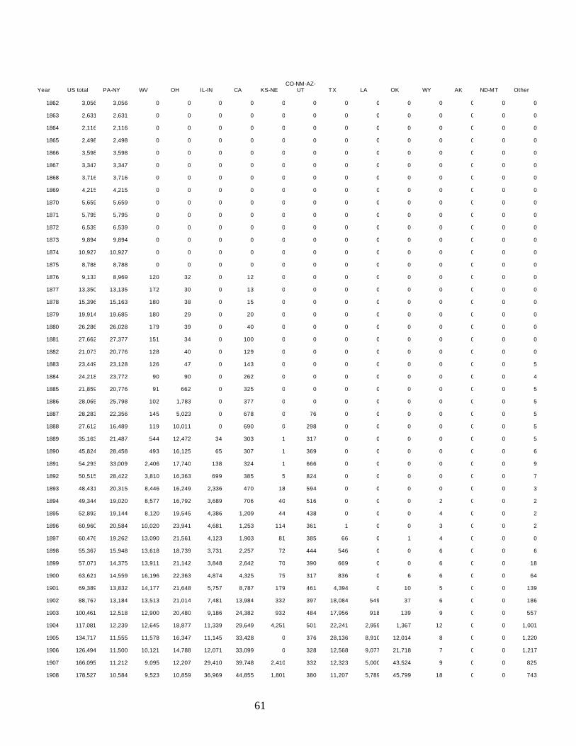
Year US total PA-NY WV OH IL-IN CA KS-NE

CO-NM-AZ-UT TX LA OK WY AK ND-MT Other

1862 3,056 3,056 0 0 0 0 0 0 0 0 0 0 0 0 0

1863 2,631 2,631 0 0 0 0 0 0 0 0 0 0 0 0 0

1864 2,116 2,116 0 0 0 0 0 0 0 0 0 0 0 0 0

1865 2,498 2,498 0 0 0 0 0 0 0 0 0 0 0 0 0

1866 3,598 3,598 0 0 0 0 0 0 0 0 0 0 0 0 0

1867 3,347 3,347 0 0 0 0 0 0 0 0 0 0 0 0 0

1868 3,716 3,716 0 0 0 0 0 0 0 0 0 0 0 0 0

1869 4,215 4,215 0 0 0 0 0 0 0 0 0 0 0 0 0

1870 5,659 5,659 0 0 0 0 0 0 0 0 0 0 0 0 0

1871 5,795 5,795 0 0 0 0 0 0 0 0 0 0 0 0 0

1872 6,539 6,539 0 0 0 0 0 0 0 0 0 0 0 0 0

1873 9,894 9,894 0 0 0 0 0 0 0 0 0 0 0 0 0

1874 10,927 10,927 0 0 0 0 0 0 0 0 0 0 0 0 0

1875 8,788 8,788 0 0 0 0 0 0 0 0 0 0 0 0 0

1876 9,133 8,969 120 32 0 12 0 0 0 0 0 0 0 0 0

1877 13,350 13,135 172 30 0 13 0 0 0 0 0 0 0 0 0

1878 15,396 15,163 180 38 0 15 0 0 0 0 0 0 0 0 0

1879 19,914 19,685 180 29 0 20 0 0 0 0 0 0 0 0 0

1880 26,286 26,028 179 39 0 40 0 0 0 0 0 0 0 0 0

1881 27,662 27,377 151 34 0 100 0 0 0 0 0 0 0 0 0

1882 21,073 20,776 128 40 0 129 0 0 0 0 0 0 0 0 0

1883 23,449 23,128 126 47 0 143 0 0 0 0 0 0 0 0 5

1884 24,218 23,772 90 90 0 262 0 0 0 0 0 0 0 0 4

1885 21,859 20,776 91 662 0 325 0 0 0 0 0 0 0 0 5

1886 28,065 25,798 102 1,783 0 377 0 0 0 0 0 0 0 0 5

1887 28,283 22,356 145 5,023 0 678 0 76 0 0 0 0 0 0 5

1888 27,612 16,489 119 10,011 0 690 0 298 0 0 0 0 0 0 5

1889 35,163 21,487 544 12,472 34 303 1 317 0 0 0 0 0 0 5

1890 45,824 28,458 493 16,125 65 307 1 369 0 0 0 0 0 0 6

1891 54,293 33,009 2,406 17,740 138 324 1 666 0 0 0 0 0 0 9

1892 50,515 28,422 3,810 16,363 699 385 5 824 0 0 0 0 0 0 7

1893 48,431 20,315 8,446 16,249 2,336 470 18 594 0 0 0 0 0 0 3

1894 49,344 19,020 8,577 16,792 3,689 706 40 516 0 0 0 2 0 0 2

1895 52,892 19,144 8,120 19,545 4,386 1,209 44 438 0 0 0 4 0 0 2

1896 60,960 20,584 10,020 23,941 4,681 1,253 114 361 1 0 0 3 0 0 2

1897 60,476 19,262 13,090 21,561 4,123 1,903 81 385 66 0 1 4 0 0 0

1898 55,367 15,948 13,618 18,739 3,731 2,257 72 444 546 0 0 6 0 0 6

1899 57,071 14,375 13,911 21,142 3,848 2,642 70 390 669 0 0 6 0 0 18

1900 63,621 14,559 16,196 22,363 4,874 4,325 75 317 836 0 6 6 0 0 64

1901 69,389 13,832 14,177 21,648 5,757 8,787 179 461 4,394 0 10 5 0 0 139

1902 88,767 13,184 13,513 21,014 7,481 13,984 332 397 18,084 549 37 6 0 0 186

1903 100,461 12,518 12,900 20,480 9,186 24,382 932 484 17,956 918 139 9 0 0 557

1904 117,081 12,239 12,645 18,877 11,339 29,649 4,251 501 22,241 2,959 1,367 12 0 0 1,001

1905 134,717 11,555 11,578 16,347 11,145 33,428 0 376 28,136 8,910 12,014 8 0 0 1,220

1906 126,494 11,500 10,121 14,788 12,071 33,099 0 328 12,568 9,077 21,718 7 0 0 1,217

1907 166,095 11,212 9,095 12,207 29,410 39,748 2,410 332 12,323 5,000 43,524 9 0 0 825

1908 178,527 10,584 9,523 10,859 36,969 44,855 1,801 380 11,207 5,789 45,799 18 0 0 743

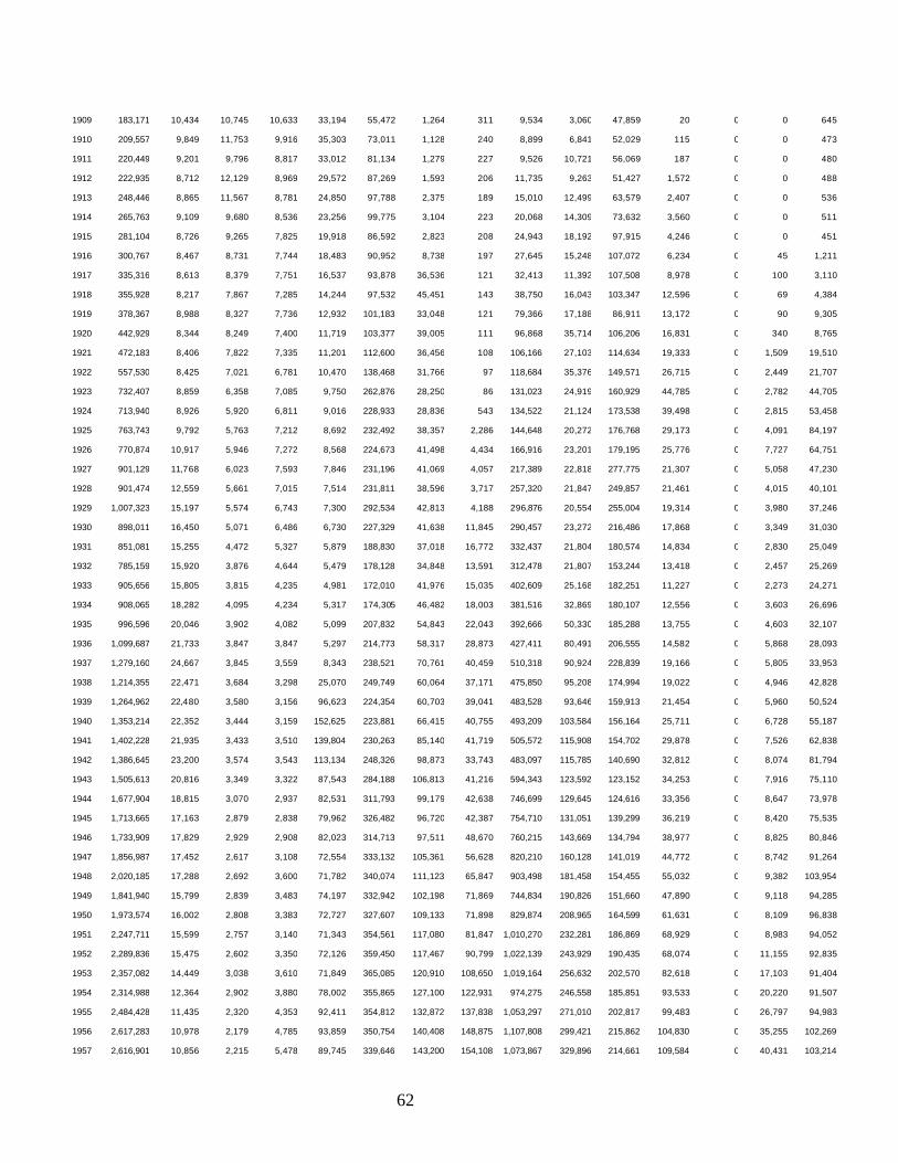
62

1909 183,171 10,434 10,745 10,633 33,194 55,472 1,264 311 9,534 3,060 47,859 20 0 0 645

1910 209,557 9,849 11,753 9,916 35,303 73,011 1,128 240 8,899 6,841 52,029 115 0 0 473

1911 220,449 9,201 9,796 8,817 33,012 81,134 1,279 227 9,526 10,721 56,069 187 0 0 480

1912 222,935 8,712 12,129 8,969 29,572 87,269 1,593 206 11,735 9,263 51,427 1,572 0 0 488

1913 248,446 8,865 11,567 8,781 24,850 97,788 2,375 189 15,010 12,499 63,579 2,407 0 0 536

1914 265,763 9,109 9,680 8,536 23,256 99,775 3,104 223 20,068 14,309 73,632 3,560 0 0 511

1915 281,104 8,726 9,265 7,825 19,918 86,592 2,823 208 24,943 18,192 97,915 4,246 0 0 451

1916 300,767 8,467 8,731 7,744 18,483 90,952 8,738 197 27,645 15,248 107,072 6,234 0 45 1,211

1917 335,316 8,613 8,379 7,751 16,537 93,878 36,536 121 32,413 11,392 107,508 8,978 0 100 3,110

1918 355,928 8,217 7,867 7,285 14,244 97,532 45,451 143 38,750 16,043 103,347 12,596 0 69 4,384

1919 378,367 8,988 8,327 7,736 12,932 101,183 33,048 121 79,366 17,188 86,911 13,172 0 90 9,305

1920 442,929 8,344 8,249 7,400 11,719 103,377 39,005 111 96,868 35,714 106,206 16,831 0 340 8,765

1921 472,183 8,406 7,822 7,335 11,201 112,600 36,456 108 106,166 27,103 114,634 19,333 0 1,509 19,510

1922 557,530 8,425 7,021 6,781 10,470 138,468 31,766 97 118,684 35,376 149,571 26,715 0 2,449 21,707

1923 732,407 8,859 6,358 7,085 9,750 262,876 28,250 86 131,023 24,919 160,929 44,785 0 2,782 44,705

1924 713,940 8,926 5,920 6,811 9,016 228,933 28,836 543 134,522 21,124 173,538 39,498 0 2,815 53,458

1925 763,743 9,792 5,763 7,212 8,692 232,492 38,357 2,286 144,648 20,272 176,768 29,173 0 4,091 84,197

1926 770,874 10,917 5,946 7,272 8,568 224,673 41,498 4,434 166,916 23,201 179,195 25,776 0 7,727 64,751

1927 901,129 11,768 6,023 7,593 7,846 231,196 41,069 4,057 217,389 22,818 277,775 21,307 0 5,058 47,230

1928 901,474 12,559 5,661 7,015 7,514 231,811 38,596 3,717 257,320 21,847 249,857 21,461 0 4,015 40,101

1929 1,007,323 15,197 5,574 6,743 7,300 292,534 42,813 4,188 296,876 20,554 255,004 19,314 0 3,980 37,246

1930 898,011 16,450 5,071 6,486 6,730 227,329 41,638 11,845 290,457 23,272 216,486 17,868 0 3,349 31,030

1931 851,081 15,255 4,472 5,327 5,879 188,830 37,018 16,772 332,437 21,804 180,574 14,834 0 2,830 25,049

1932 785,159 15,920 3,876 4,644 5,479 178,128 34,848 13,591 312,478 21,807 153,244 13,418 0 2,457 25,269

1933 905,656 15,805 3,815 4,235 4,981 172,010 41,976 15,035 402,609 25,168 182,251 11,227 0 2,273 24,271

1934 908,065 18,282 4,095 4,234 5,317 174,305 46,482 18,003 381,516 32,869 180,107 12,556 0 3,603 26,696

1935 996,596 20,046 3,902 4,082 5,099 207,832 54,843 22,043 392,666 50,330 185,288 13,755 0 4,603 32,107

1936 1,099,687 21,733 3,847 3,847 5,297 214,773 58,317 28,873 427,411 80,491 206,555 14,582 0 5,868 28,093

1937 1,279,160 24,667 3,845 3,559 8,343 238,521 70,761 40,459 510,318 90,924 228,839 19,166 0 5,805 33,953

1938 1,214,355 22,471 3,684 3,298 25,070 249,749 60,064 37,171 475,850 95,208 174,994 19,022 0 4,946 42,828

1939 1,264,962 22,480 3,580 3,156 96,623 224,354 60,703 39,041 483,528 93,646 159,913 21,454 0 5,960 50,524

1940 1,353,214 22,352 3,444 3,159 152,625 223,881 66,415 40,755 493,209 103,584 156,164 25,711 0 6,728 55,187

1941 1,402,228 21,935 3,433 3,510 139,804 230,263 85,140 41,719 505,572 115,908 154,702 29,878 0 7,526 62,838

1942 1,386,645 23,200 3,574 3,543 113,134 248,326 98,873 33,743 483,097 115,785 140,690 32,812 0 8,074 81,794

1943 1,505,613 20,816 3,349 3,322 87,543 284,188 106,813 41,216 594,343 123,592 123,152 34,253 0 7,916 75,110

1944 1,677,904 18,815 3,070 2,937 82,531 311,793 99,179 42,638 746,699 129,645 124,616 33,356 0 8,647 73,978

1945 1,713,665 17,163 2,879 2,838 79,962 326,482 96,720 42,387 754,710 131,051 139,299 36,219 0 8,420 75,535

1946 1,733,909 17,829 2,929 2,908 82,023 314,713 97,511 48,670 760,215 143,669 134,794 38,977 0 8,825 80,846

1947 1,856,987 17,452 2,617 3,108 72,554 333,132 105,361 56,628 820,210 160,128 141,019 44,772 0 8,742 91,264

1948 2,020,185 17,288 2,692 3,600 71,782 340,074 111,123 65,847 903,498 181,458 154,455 55,032 0 9,382 103,954

1949 1,841,940 15,799 2,839 3,483 74,197 332,942 102,198 71,869 744,834 190,826 151,660 47,890 0 9,118 94,285

1950 1,973,574 16,002 2,808 3,383 72,727 327,607 109,133 71,898 829,874 208,965 164,599 61,631 0 8,109 96,838

1951 2,247,711 15,599 2,757 3,140 71,343 354,561 117,080 81,847 1,010,270 232,281 186,869 68,929 0 8,983 94,052

1952 2,289,836 15,475 2,602 3,350 72,126 359,450 117,467 90,799 1,022,139 243,929 190,435 68,074 0 11,155 92,835

1953 2,357,082 14,449 3,038 3,610 71,849 365,085 120,910 108,650 1,019,164 256,632 202,570 82,618 0 17,103 91,404

1954 2,314,988 12,364 2,902 3,880 78,002 355,865 127,100 122,931 974,275 246,558 185,851 93,533 0 20,220 91,507

1955 2,484,428 11,435 2,320 4,353 92,411 354,812 132,872 137,838 1,053,297 271,010 202,817 99,483 0 26,797 94,983

1956 2,617,283 10,978 2,179 4,785 93,859 350,754 140,408 148,875 1,107,808 299,421 215,862 104,830 0 35,255 102,269

1957 2,616,901 10,856 2,215 5,478 89,745 339,646 143,200 154,108 1,073,867 329,896 214,661 109,584 0 40,431 103,214

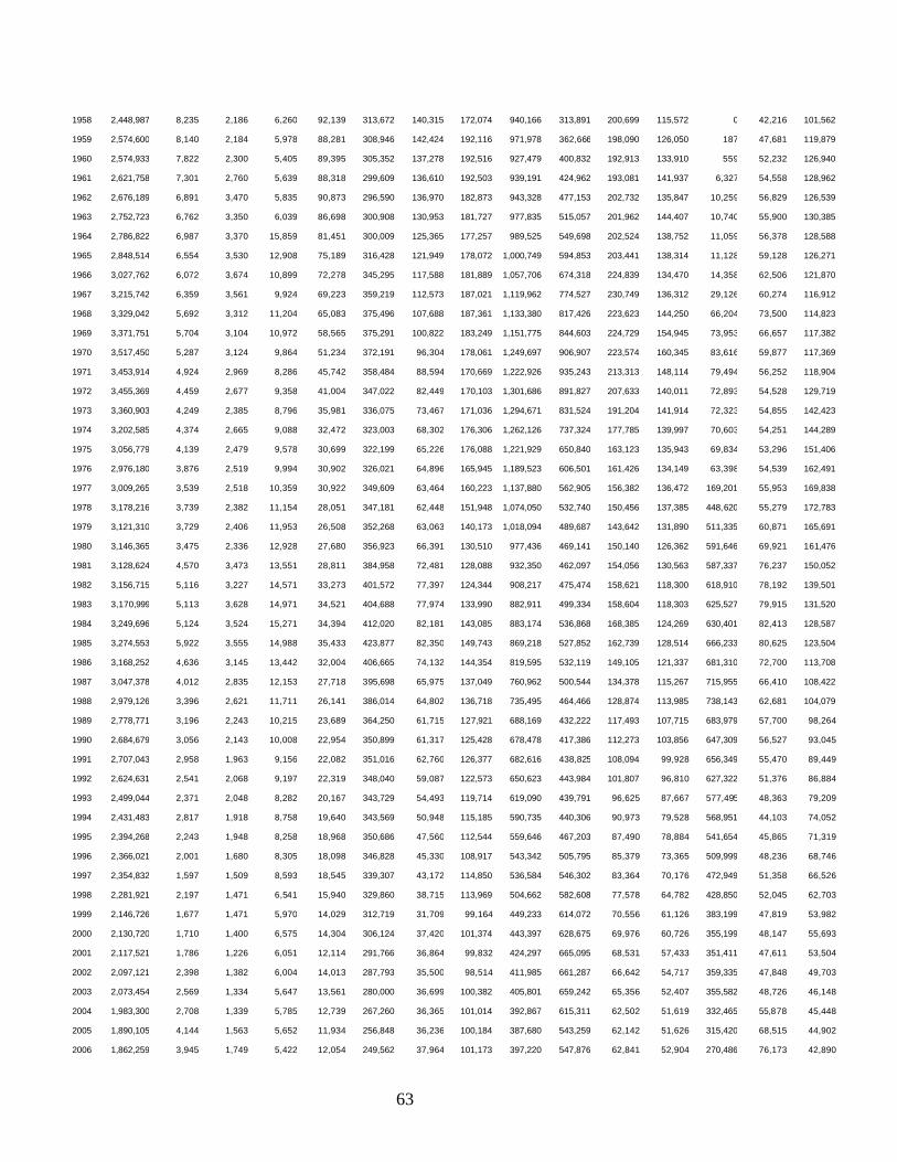
63

1958 2,448,987 8,235 2,186 6,260 92,139 313,672 140,315 172,074 940,166 313,891 200,699 115,572 0 42,216 101,562

1959 2,574,600 8,140 2,184 5,978 88,281 308,946 142,424 192,116 971,978 362,666 198,090 126,050 187 47,681 119,879

1960 2,574,933 7,822 2,300 5,405 89,395 305,352 137,278 192,516 927,479 400,832 192,913 133,910 559 52,232 126,940

1961 2,621,758 7,301 2,760 5,639 88,318 299,609 136,610 192,503 939,191 424,962 193,081 141,937 6,327 54,558 128,962

1962 2,676,189 6,891 3,470 5,835 90,873 296,590 136,970 182,873 943,328 477,153 202,732 135,847 10,259 56,829 126,539

1963 2,752,723 6,762 3,350 6,039 86,698 300,908 130,953 181,727 977,835 515,057 201,962 144,407 10,740 55,900 130,385

1964 2,786,822 6,987 3,370 15,859 81,451 300,009 125,365 177,257 989,525 549,698 202,524 138,752 11,059 56,378 128,588

1965 2,848,514 6,554 3,530 12,908 75,189 316,428 121,949 178,072 1,000,749 594,853 203,441 138,314 11,128 59,128 126,271

1966 3,027,762 6,072 3,674 10,899 72,278 345,295 117,588 181,889 1,057,706 674,318 224,839 134,470 14,358 62,506 121,870

1967 3,215,742 6,359 3,561 9,924 69,223 359,219 112,573 187,021 1,119,962 774,527 230,749 136,312 29,126 60,274 116,912

1968 3,329,042 5,692 3,312 11,204 65,083 375,496 107,688 187,361 1,133,380 817,426 223,623 144,250 66,204 73,500 114,823

1969 3,371,751 5,704 3,104 10,972 58,565 375,291 100,822 183,249 1,151,775 844,603 224,729 154,945 73,953 66,657 117,382

1970 3,517,450 5,287 3,124 9,864 51,234 372,191 96,304 178,061 1,249,697 906,907 223,574 160,345 83,616 59,877 117,369

1971 3,453,914 4,924 2,969 8,286 45,742 358,484 88,594 170,669 1,222,926 935,243 213,313 148,114 79,494 56,252 118,904

1972 3,455,369 4,459 2,677 9,358 41,004 347,022 82,449 170,103 1,301,686 891,827 207,633 140,011 72,893 54,528 129,719

1973 3,360,903 4,249 2,385 8,796 35,981 336,075 73,467 171,036 1,294,671 831,524 191,204 141,914 72,323 54,855 142,423

1974 3,202,585 4,374 2,665 9,088 32,472 323,003 68,302 176,306 1,262,126 737,324 177,785 139,997 70,603 54,251 144,289

1975 3,056,779 4,139 2,479 9,578 30,699 322,199 65,226 176,088 1,221,929 650,840 163,123 135,943 69,834 53,296 151,406

1976 2,976,180 3,876 2,519 9,994 30,902 326,021 64,896 165,945 1,189,523 606,501 161,426 134,149 63,398 54,539 162,491

1977 3,009,265 3,539 2,518 10,359 30,922 349,609 63,464 160,223 1,137,880 562,905 156,382 136,472 169,201 55,953 169,838

1978 3,178,216 3,739 2,382 11,154 28,051 347,181 62,448 151,948 1,074,050 532,740 150,456 137,385 448,620 55,279 172,783

1979 3,121,310 3,729 2,406 11,953 26,508 352,268 63,063 140,173 1,018,094 489,687 143,642 131,890 511,335 60,871 165,691

1980 3,146,365 3,475 2,336 12,928 27,680 356,923 66,391 130,510 977,436 469,141 150,140 126,362 591,646 69,921 161,476

1981 3,128,624 4,570 3,473 13,551 28,811 384,958 72,481 128,088 932,350 462,097 154,056 130,563 587,337 76,237 150,052

1982 3,156,715 5,116 3,227 14,571 33,273 401,572 77,397 124,344 908,217 475,474 158,621 118,300 618,910 78,192 139,501

1983 3,170,999 5,113 3,628 14,971 34,521 404,688 77,974 133,990 882,911 499,334 158,604 118,303 625,527 79,915 131,520

1984 3,249,696 5,124 3,524 15,271 34,394 412,020 82,181 143,085 883,174 536,868 168,385 124,269 630,401 82,413 128,587

1985 3,274,553 5,922 3,555 14,988 35,433 423,877 82,350 149,743 869,218 527,852 162,739 128,514 666,233 80,625 123,504

1986 3,168,252 4,636 3,145 13,442 32,004 406,665 74,132 144,354 819,595 532,119 149,105 121,337 681,310 72,700 113,708

1987 3,047,378 4,012 2,835 12,153 27,718 395,698 65,975 137,049 760,962 500,544 134,378 115,267 715,955 66,410 108,422

1988 2,979,126 3,396 2,621 11,711 26,141 386,014 64,802 136,718 735,495 464,466 128,874 113,985 738,143 62,681 104,079

1989 2,778,771 3,196 2,243 10,215 23,689 364,250 61,715 127,921 688,169 432,222 117,493 107,715 683,979 57,700 98,264

1990 2,684,679 3,056 2,143 10,008 22,954 350,899 61,317 125,428 678,478 417,386 112,273 103,856 647,309 56,527 93,045

1991 2,707,043 2,958 1,963 9,156 22,082 351,016 62,760 126,377 682,616 438,825 108,094 99,928 656,349 55,470 89,449

1992 2,624,631 2,541 2,068 9,197 22,319 348,040 59,087 122,573 650,623 443,984 101,807 96,810 627,322 51,376 86,884

1993 2,499,044 2,371 2,048 8,282 20,167 343,729 54,493 119,714 619,090 439,791 96,625 87,667 577,495 48,363 79,209

1994 2,431,483 2,817 1,918 8,758 19,640 343,569 50,948 115,185 590,735 440,306 90,973 79,528 568,951 44,103 74,052

1995 2,394,268 2,243 1,948 8,258 18,968 350,686 47,560 112,544 559,646 467,203 87,490 78,884 541,654 45,865 71,319

1996 2,366,021 2,001 1,680 8,305 18,098 346,828 45,330 108,917 543,342 505,795 85,379 73,365 509,999 48,236 68,746

1997 2,354,832 1,597 1,509 8,593 18,545 339,307 43,172 114,850 536,584 546,302 83,364 70,176 472,949 51,358 66,526

1998 2,281,921 2,197 1,471 6,541 15,940 329,860 38,715 113,969 504,662 582,608 77,578 64,782 428,850 52,045 62,703

1999 2,146,726 1,677 1,471 5,970 14,029 312,719 31,709 99,164 449,233 614,072 70,556 61,126 383,199 47,819 53,982

2000 2,130,720 1,710 1,400 6,575 14,304 306,124 37,420 101,374 443,397 628,675 69,976 60,726 355,199 48,147 55,693

2001 2,117,521 1,786 1,226 6,051 12,114 291,766 36,864 99,832 424,297 665,095 68,531 57,433 351,411 47,611 53,504

2002 2,097,121 2,398 1,382 6,004 14,013 287,793 35,500 98,514 411,985 661,287 66,642 54,717 359,335 47,848 49,703

2003 2,073,454 2,569 1,334 5,647 13,561 280,000 36,699 100,382 405,801 659,242 65,356 52,407 355,582 48,726 46,148

2004 1,983,300 2,708 1,339 5,785 12,739 267,260 36,365 101,014 392,867 615,311 62,502 51,619 332,465 55,878 45,448

2005 1,890,105 4,144 1,563 5,652 11,934 256,848 36,236 100,184 387,680 543,259 62,142 51,626 315,420 68,515 44,902

2006 1,862,259 3,945 1,749 5,422 12,054 249,562 37,964 101,173 397,220 547,876 62,841 52,904 270,486 76,173 42,890

64

2007 1,848,452 4,033 1,574 5,455 11,336 241,378 38,824 101,631 396,894 542,763 60,952 54,130 263,595 79,887 46,000

2008 1,811,819 3,997 1,593 5,715 11,281 238,691 41,976 105,507 398,014 494,708 64,065 52,943 249,874 94,321 49,134

2009 1,956,597 3,880 1,864 5,834 10,903 228,994 41,703 112,443 403,797 638,004 67,018 51,333 235,500 107,428 47,896

2010 1,998,138 3,923 1,992 4,785 10,901 223,501 42,672 120,583 426,700 633,639 69,513 53,133 218,762 138,341 49,693

Documents

Oil Prices, Exhaustible Resources, and Economic Growth*econweb.ucsd.edu/~jhamilto/handbook_climate.pdf · Oil Prices, Exhaustible Resources, and Economic ... real price of crude petroleum