OH et al.: A SCALABLE REAL-TIME MULTIPLE-TARGET TRACKING ALGORITHM FOR SENSOR NETWORKS ...robotics.eecs.berkeley.edu/~sastry/pubs/PDFs of Pubs2000... · 2005-10-13 · OH et al.:

OH et al.: A SCALABLE REAL-TIME MULTIPLE-TARGET TRACKING ALGORITHM FOR SENSOR NETWORKS 1

A Scalable Real-Time Multiple-Target Tracking

Algorithm for Sensor Networks

Songhwai Oh, Luca Schenato, Phoebus Chen, and Shankar Sastry

Abstract

Multiple-target tracking is a representative real-time application of sensor networks as it exhibits

different aspects of sensor networks such as event detection, sensor information fusion, multi-hop

communication, sensor management and real-time decision making. The task of tracking multiple objects

in a sensor network is challenging due to constraints on a sensor node such as short communication

and sensing ranges, a limited amount of memory and limited computational power. In addition, since a

sensor network surveillance system needs to operate autonomously without human operators, it requires

an autonomous real-time tracking algorithm which can track an unknown number of targets. In this

paper, we develop a scalable real-time multiple-target tracking algorithm that is autonomous and robust

against transmission failures, communication delays and sensor localization error. In particular, there is

no performance loss up to the average localization error of.7 times the separation between sensors and

the algorithm tolerates up to 50% lost-to-total packet ratio and 90% delayed-to-total packet ratio.

I. I NTRODUCTION

In wireless ad-hoc sensor networks, many inexpensive and small sensor-rich devices are

deployed to monitor and control our environment [7], [9]. Each device, called a sensor node,

is capable of sensing, computation and communication. Sensor nodes form a wireless ad-

hoc network for communication. The limited supply of power and other constraints, such as

Songhwai Oh, Phoebus Chen, and Shankar Sastry are with the Department of Electrical Engineering and Computer Sciences,

University of California, Berkeley, CA 94720,sho,phoebusc,sastry @eecs.berkeley.edu .

Luca Schenato is with the Department of Information Engineering, University of Padova, Via Gradenigo 6/B, 31100 Padova,

Italy. [email protected] .

This material is based upon work supported by the National Science Foundation under Grant No. EIA-0122599 and by the

European Community Research Information Society Technologies under Grant No. RECSYS IST-2001-32515.


manufacturing costs and limited package sizes, limit the capabilities of each sensor node. For

example, a typical sensor node has short communication and sensing ranges, a limited amount

of memory and limited computational power. However, the abundant number of spatially spread

sensors will enable us to monitor changes in our environment accurately despite the inaccuracy

of each sensor node.

Multiple-target tracking is a representative real-time application of sensor networks as it

exhibits different aspects of sensor networks such as event detection, sensor information fusion,

communication, sensor management, and real-time decision making. The applications of tracking

using sensor networks include surveillance, search and rescue, disaster response system, pursuit

evasion games [25], distributed control [27], spatio-temporal data collection, and other location-

based services [10]. However, the task of tracking multiple objects in a sensor network is

challenging due to the following issues. Each sensor node has a limited supply of power,

leading to low detection probability and high false alarm rate. The presence of false alarms

and missing observations complicate the problems of track initiation and termination. These

important issues are ignored by many tracking algorithm designed for sensor networks. For

example, when the false alarm rate is high, a naive track initiation algorithm will overflow the

network with spurious tracks. Hence, an algorithm for sensor networks must be robust against the

low detection probability and high false alarm rate. To conserve power and reduce interference,

multi-hop routing is used in sensor networks. In many cases, the communication links are not

reliable, causing transmission failures. In addition, due to the low communication bandwidth

and a limited amount of memory, communication delays can occur frequently. Moreover, the

localization of sensor nodes in an ad-hoc wireless sensor network without expensive hardware

such as the global positioning system (GPS) is a challenging problem [28]. Since the position

of a target is reported with respect to the location of the reporting sensor, the algorithm must be

robust against the sensor localization error. It is well known that communication is costlier than

computation in sensor networks in terms of power usage [8]. Hence, it is essential to fuse local

observations before the transmission. However, since the data association problem of multiple-

target tracking is NP-hard [22], we cannot expect to solve it with only local information. But

at the same time we cannot afford to have a centralized algorithm since such a solution is not

scalable. Lastly, in sensor networks, we seek for an autonomous tracking algorithm which does

not require a continuous monitoring by a human operator.


In summary, we need a real-time tracking algorithm that is robust against the low detection

probability and high false alarm rates; capable of initiating and terminating tracks; uses less

memory; combines local information to reduce the communication load; and is scalable. Also it

must be robust against transmission failures, communication delays and sensor localization error.

But at the same time we want an algorithm that provides a good solution which approaches the

optimum given enough computation time.

In [20], Markov chain Monte Carlo data association (MCMCDA) is presented. MCMCDA

can track an unknown number of targets in real-time and is an approximation to the optimal

Bayesian filter. It has been shown that MCMCDA is computationally efficient compared to the

multiple hypothesis tracker (MHT) [23] and outperforms MHT under extreme conditions, such

as a large number of targets in a dense environment, low detection probabilities, and high false

alarm rates [20]. MCMCDA is suitable for sensor networks since it can autonomously initiate and

terminate tracks. Since transmission failure is another form of a missing observation, MCMCDA

is robust against transmission failures. MCMCDA performs data association based on both

current and past observations, so delayed observations,i.e., out-of-sequence measurements, can

be easily combined with previously received observations to improve the accuracy of estimates.

Furthermore, MCMCDA requires less memory as it maintains only the current hypothesis and

the hypothesis with the highest posterior. It does not require the enumeration of all or some

of hypotheses as in [23], [14]. In this paper, we extend the MCMCDA algorithm to sensor

networks in a hierarchical manner so that the algorithm becomes scalable. To our knowledge,

the algorithm presented in this paper is the first general real-time scalable multiple-target tracking

algorithm for sensor networks which can systematically track an unknown number of targets in

the presence of false alarms and missing observations and is robust against transmission failures,

communication delays and sensor localization error.

We consider a simple shortest-path routing scheme on a sensor network. The transmission

failures and communication delays of the network are characterized probabilistically. We assume

the availability of a small number of special nodes,supernodes, that are more capable than regular

nodes in terms of computational power and communication range. Each node is assigned to its

nearest supernode and nodes are grouped by supernodes. We call the group of sensor nodes

formed around a supernode as a “tracking group”. When a node detects a possible target, it

communicates with its neighbors and observations from the neighboring sensors are fused and


sent to its supernode. Each supernode receives the fused observations from its tracking group

and executes the tracking algorithm. Each supernode communicates with neighboring supernodes

when a target moves away from its range. Lastly, the tracks estimated by supernodes are combined

hierarchically. Although a specific sensor network model is used for the performance evaluation,

the algorithm is applicable for different routing algorithms and sensor models,e.g., distributed

air traffic control [19].

The remainder of this paper is structured as follows. In Section III, the multiple-target tracking

problem and its probabilistic model are described. The MCMCDA algorithm for multiple-target

tracking is presented in Section IV. The sensor network model is described in Section V and the

hierarchical MCMCDA method is given in Section VI. The simulation and experiment results

are shown in Section VII and VIII.

II. RELATED WORK

The general-purpose multiple-target tracking algorithms such as the joint probabilistic data

association filter (JPDAF) [1] and multiple hypothesis tracker (MHT) [23] are robust against the

low detection probability and high false alarm rate. But they are not suitable for sensor networks

since track initiation and termination is difficult with JPDAF and both JPDAF and MHT require

large memory and computation cycles. Since MHT can initiate and terminate tracks, the tracking

task can be easily distributed in a network of sensors. In [5], a distributed tracking algorithm

based on MHT is developed for multiple sensors. But the approach is not suitable for sensor

networks since it demands large computational power and a large amount of memory on each

sensor.

In [15], the authors propose to use a classification algorithm to disambiguate closely located

targets. But signals received from targets are correlated and we cannot recover the uncorrelated

signals in all cases. Since we do not know in advance the number of targets around each sensor,

the problem is ill-posed and very challenging even for a high-end computer.

In [17], distributed track initiation and maintenance methods are described. By electing a

leader among the sensors by which a target is detected, unnecessary communication is reduced

while tracking targets using the nearest neighbor method. But considering the complexity of the

data association problem, the approach will suffer from incorrect associations when there are

many targets crossing or moving close to each other. In addition, when the false alarm rate is


high, the proposed approach will overflow the network with spurious tracks and it is unclear

how the missing observations are handled.

Recently, some multiple-target tracking algorithms specifically designed for sensor networks

have been proposed to solve the identity management problem [26], [16]. They assume the

availability of a classification algorithm as in [15] but the disambiguation is delayed until targets

are sufficiently separated. As assumed in the simulations of [16], when the targets are of different

classes, a target can be classified by the signature of its class. But, if all targets are of the

same class, a target cannot be easily classified by its signature and, in the absence of reliable

classification information, the proposed methods will behave like the naive nearest neighbor

tracker. Our algorithm can complement the identity management algorithms when tracking targets

within the same class or when reliable classification information is not available.

A distributed particle filtering algorithm for sensor networks is presented in [6] and used to

track a single maneuvering target, assuming the availability of supernodes and a hierarchical

topology similar to ours. The paper assumes the availability of sensors which can measure an

angle and distance to a target. But sensors with such capabilities are costly and they are not

suitable for a large sensor network with inexpensive sensor nodes. The most widely used and

realistic sensor model is based on the signal strength and this is the model we use in this paper.

III. M ULTIPLE-TARGET TRACKING

A. Problem Formulation

Let T ∈ Z+ be the duration of surveillance. LetK be the unknown number of objects moving

around the surveillance regionR for some duration[tki , tkf ] ⊂ [1, T ] for k = 1, . . . , K. Let V be

the volume ofR. Each object arises at a random position inR at tki , moves independently around

R until tkf and disappears. At each time, an existing target persists with probability1− pz and

disppears with probabilitypz. The number of objects arising at each time overR has a Poisson

distribution with a parameterλbV whereλb is the birth rate of new objects per unit time, per

unit volume. The initial position of a new object is uniformly distributed overR.

Let F k : Rnx → Rnx be the discrete-time dynamics of the objectk, wherenx is the dimension

of the state variable, and letxkt ∈ Rnx be the state of the objectk at time t for k = 1, . . . , K.

The objectk moves according to

xkt+1 = F k(xk

t ) + wkt , for t = tki , . . . , t

kf − 1, (1)


wherewkt ∈ Rnx are white noise processes. The white noise process is included to model non-

rectilinear motions of targets. The noisy observation of the state of the object is measured with a

detection probabilitypd which is less than unity. There are also false alarms and the number of

false alarms has a Poisson distribution with a parameterλfV whereλf is the false alarm rate per

unit time, per unit volume. Letnt be the number of observations at timet, including both noisy

observations and false alarms. Letyjt ∈ Rny be thej-th observation at timet for j = 1, . . . , nt,

whereny is the dimension of each observation vector. Each object generates a unique observation

at each sampling time if it is detected. LetHj : Rnx → Rny be the observation model. Then the

observations are generated as follows:

yjt =

Hj(xkt ) + vj

t if j-th observation is fromxkt

ut otherwise,(2)

where vjt ∈ Rny are white noise processes andut ∼ Unif(R) is a random process for false

alarms. Notice that, with probability1− pd, the object is not detected and we call this a missing

observation. We assume that targets are indistinguishable in this paper. But, if observations

include target type or attribute information, the state variable can be extended to include target

type information. The multiple-target tracking problem is to estimateK from measurements as

well as tki , tkf andxkt for tki ≤ t ≤ tkf andk = 1, . . . , K.

B. A Solution to the Multiple-Target Tracking Problem

Let yt = yjt : j = 1, . . . , nt andY = yt : 1 ≤ t ≤ T. Let Ω be a collection of partitions

of Y such that, forω ∈ Ω,

1) ω = τ0, τ1, . . . , τK;

2)⋃K

k=0 τk = Y andτi ∩ τj = ∅ for i 6= j;

3) τ0 is a set of false alarms;

4) |τk ∩ yt| ≤ 1 for k = 1, . . . , K and t = 1, . . . , T ; and

5) |τk| ≥ 2 for k = 1, . . . , K.

Here,K is the number of tracks for the given partitionω ∈ Ω and |τk| denotes the cardinality

of the setτk. We call τk a track when there is no confusion although the actual track is the

set of estimated states from the observationsτk. However, we assume there is a deterministic

function that returns a set of estimated states given a set of observations, so no distinction is


Fig. 1. (a) An example of observationsY (each circle represents an observation and numbers represent observation times). (b)

An example of a partitionω of Y

required. The fourth requirement says that a track can have at most one observation at each time,

but, in the case of multiple sensors with overlapping sensing regions, we can easily relax this

requirement to allow multiple observations per track. A track is assumed to contain at least two

observations since we cannot distinguish a track with a single observation from a false alarm.

An example of a partition is shown in Figure 1.

Let et be the number of targets from timet− 1 andat be the number of new targets at time

t. Let zt be the number of targets terminated at timet andct = et− zt be the number of targets

from time t− 1 that have not terminated at timet. Let dt be the number of detections at time

t and ut = ct + at − dt be the number of undetected targets. Finally, letft = nt − dt be the

number of false alarms. It can be shown that the posterior ofω is:

P (ω|Y ) ∝∏T

t=1 pztz (1− pz)

ctpdtd (1− pd)

utλatb λft

f P (Y |ω) (3)

where P (Y |ω) is the likelihood of observationsY given ω, which can be computed based

on the chosen dynamic and measurement models. One solution to the multiple-target tracking

problem is to find a partition of measurements such thatP (ω|Y ) is maximized,i.e., a maximum

a posteriori (MAP) estimate.

IV. M ARKOV CHAIN MONTE CARLO DATA ASSOCIATIONALGORITHM

In this section, we develop an MCMC sampler to solve the multiple-target tracking prob-

lem. MCMC-based algorithms play a significant role in many fields such as physics, statistics,

economics, and engineering [2]. In some cases, MCMC is the only known general algorithm

that finds a good approximate solution to a complex problem in polynomial time [13]. MCMC


techniques have been applied to complex probability distribution integration problems, counting

problems such as #P-complete problems, and combinatorial optimization problems [13], [2].

MCMC is a general method to generate samples from a distributionπ by constructing a

Markov chainM whose states areω and whose stationary distribution isπ(ω). If we are at state

ω ∈ Ω, we proposeω′ ∈ Ω following the proposal distributionq(ω, ω′). The move is accepted

with an acceptance probabilityA(ω, ω′) where

A(ω, ω′) = min

(1,

π(ω′)q(ω′, ω)

π(ω)q(ω, ω′)

), (4)

otherwise the sampler stays atω, so that the detailed balance is satisfied. If we make sure that

M is irreducible and aperiodic, thenM converges to its stationary distribution by the ergodic

theorem [24].

Algorithm 1 MCMCDAInput : Y, nmc, ωinit

Output : ω

ω = ω ← ωinit

for n = 1 to nmc do

proposeω′ based onω (see [20])

sampleU from Unif[0, 1]

ω ← ω′ if U < A(ω, ω′)

ω ← ω if p(ω|Y )/p(ω|Y ) > 1

end for

The MCMC data association (MCMCDA) algorithm is described in Algorithm 1. MCMCDA

is an MCMC algorithm whose state space isΩ described in Section III-B and whose stationary

distribution is the posterior (3). The proposal distribution for MCMCDA consists of five types

of moves. They are (1) birth/death move pair; (2) split/merge move pair; (3) extension/reduction

move pair; (4) track update move; and (5) track switch move. The MCMCDA moves are

graphically illustrated in Figure 2. For a detailed description of each move, see [20]. The inputs

for MCMCDA are the set of all observationsY , the number of samplesnmc, and the initial state

ωinit. The acceptance probabilityA(ω, ω′) is defined in (4) whereπ(ω) = P (ω|Y ) from (3). In


Fig. 2. Graphical illustration of MCMCDA moves (associations are indicated by dotted lines and hollow circles are false

alarms)

Algorithm 1, we use MCMC to find a solution to a combinatorial optimization problem. So it

can be considered as simulated annealing at a constant temperature.

In addition, the memory requirement of the algorithm is at its bare minimum. Instead of

keeping allω(n)nmcn=1, we simply keep the partition with the maximum posterior,ω. Notice

that, in MCMC, the construction ofω′ is done on the fly according to the proposal distribution

q(ω, ω′) and there is no need to store previously visited states.

The Markov chain designed by Algorithm 1 is irreducible and aperiodic [20]. In addition,

the transitions described in Algorithm 1 satisfy the detailed balance condition since it uses

the Metropolis-Hastings kernel (4). Hence, by the ergodic theorem, the chain converges to its

stationary distribution [24].

V. SENSORNETWORK MODEL

In this section, we describe the sensor network and sensor model used in simulations in

Section VII. Let Ns be the number of sensor nodes, including both supernodes and regular

nodes, deployed over the surveillance regionR ⊂ R2. We assume that each supernode can

communicate with its neighboring supernodes. Letsi ∈ R be the location of thei-th sensor

node and letS = si : 1 ≤ i ≤ Ns. Let G = (S, E) be a communication graph such that

(si, sj) ∈ E if and only if nodei can communicate with nodej. Let Nss Ns be the number

of supernodes and letssj ∈ S be the position of thej-th supernode, forj = 1, . . . , Nss. Let

g : 1, . . . , Ns → 1, . . . , Nss be the assignment of each sensor to its nearest supernode such

that g(i) = j if ‖si − ssj‖ = mink=1,...,Nss‖si − ss

k‖. For a nodei, if g(i) = j, the shortest path


from si to ssj in G is denoted bysp(i). For each supernodej, its tracking group contains a set

of nodessi ∈ S : g(i) = j.

Let Rs ∈ R be the sensing range. If there is an object atx ∈ R, a sensor can detect the

presence of the object. Each sensor records the sensor’s signal strength,

zi =

β1+γ‖si−x‖α + ws

i , if ‖si − x‖ ≤ Rs

wsi , if ‖si − x‖ > Rs,

(5)

whereα, β andγ are constants specific to the sensor type, and we assume thatzi are normalized

such thatwsi has the standard Gaussian distribution. This signal-strength based sensor model (5)

is general for sensors available in sensor networks, such as acoustic and magnetic sensors, and

has been used frequently [16], [17], [18]. For eachi, if zi ≥ η, where η is a threshold set

for appropriate values of detection and false-positive probabilities, the node transmitszi to its

neighboring nodes, which are at most2Rs away fromsi, and listens to incoming messages from

its 2Rs neighborhood. Note that this approach is similar to the leader election scheme in [17]

and we assume that the transmission range of each node is larger than2Rs. For the nodei, if

zi is the larger than all incoming messages,zi1 , . . . , zik−1, andzik = zi, then the position of an

object is estimated as

zi =

∑kj=1 zijsij∑k

j=1 zij

. (6)

The estimatezi corresponds to the computation of a center of mass of the sensing nodes weighed

by measured signal strengths. The nodei transmitszi to the supernodeg(i) via the shortest path

sp(i). If zi is not the largest compared to the incoming messages, the nodei does nothing and

goes back to the sensing mode. Although each sensor cannot give an accurate estimate of object’s

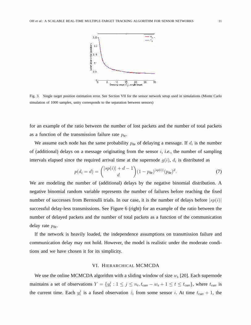
position, as more sensors collaborate, the accuracy of estimates improves as shown in Figure 3.

A transmission along the edge(si, sj) fails independently with probabilitypte and the message

never reaches a supernode. Notice that the transmission failure includes failures from retrans-

missions. We can consider transmission failure as another form of a missing observation. Ifk is

the number of hops required to relay data from a sensor node to its supernode, the probability of

successful transmission decays exponentially ask increases. To overcome this problem, we use

k independent paths to relay data if the reporting sensor node isk hops away from its supernode.

The probability of successful communicationpts from the reporting nodei to its supernodeg(i)

can be computed aspts(pte, k) = 1 −(1− (1− pte)

k)k

, wherek = |sp(i)|. See Figure 6 (left)


Fig. 3. Single target position estimation error. See Section VII for the sensor network setup used in simulations (Monte Carlo

simulation of 1000 samples, unity corresponds to the separation between sensors)

for an example of the ratio between the number of lost packets and the number of total packets

as a function of the transmission failure ratepte.

We assume each node has the same probabilitypde of delaying a message. Ifdi is the number

of (additional) delays on a message originating from the sensori, i.e., the number of sampling

intervals elapsed since the required arrival time at the supernodeg(i), di is distributed as

p(di = d) =

(|sp(i)|+ d− 1

d

)(1− pde)

|sp(i)|(pde)d. (7)

We are modeling the number of (additional) delays by the negative binomial distribution. A

negative binomial random variable represents the number of failures before reaching the fixed

number of successes from Bernoulli trials. In our case, it is the number of delays before|sp(i)|

successful delay-less transmissions. See Figure 6 (right) for an example of the ratio between the

number of delayed packets and the number of total packets as a function of the communication

delay ratepde.

If the network is heavily loaded, the independence assumptions on transmission failure and

communication delay may not hold. However, the model is realistic under the moderate condi-

tions and we have chosen it for its simplicity.

VI. H IERARCHICAL MCMCDA

We use the online MCMCDA algorithm with a sliding window of sizews [20]. Each supernode

maintains a set of observationsY = yjt : 1 ≤ j ≤ nt, tcurr− ws + 1 ≤ t ≤ tcurr, wheretcurr is

the current time. Eachyjt is a fused observationzi from some sensori. At time tcurr + 1, the


observations at timetcurr−ws+1 are removed fromY and a new set of observations is appended to

Y . Any delayed observations are appended to appropriate slots. Then each supernode initializes

the Markov chain with the previously estimated tracks and executes Algorithm 1 onY . Once

tracks are found, the next state of each track is predicted. If the predicted next state belongs

to the surveillance area of another supernode, track information is passed to the corresponding

supernode. The newly received tracks are incorporated into the initial state of MCMCDA for

the next time step.

Since each supernode maintains its own set of tracks, there can be multiple tracks from a

single object maintained by different supernodes. To make the algorithm fully hierarchical, we

do track-level data association to combine tracks from different supernodes. Letωj be the set

of tracks maintained by supernodej ∈ 1, . . . , Nss. Let Yc = τi(t) ∈ ωj : 1 ≤ t ≤ T, 1 ≤

i ≤ |ωj|, 1 ≤ j ≤ Nss be the combined observations only from the established tracks. We form

a new set of tracksωinit from τi ∈ ωj : 1 ≤ i ≤ |ωj|, 1 ≤ j ≤ Nss while making sure that

constraints defined in Section III-B are satisfied. Then we run Algorithm 1 on this combined

observation setYc with the initial stateωinit. An example in which the track-level data association

step corrects mistakes made by supernodes due to missing observations at the tracking group

boundaries is shown in [21].

VII. S IMULATION RESULTS

For simulations below, we consider the surveillance over a rectangular region on a plane,

R = [0, 100]2. The state vector isx = [x1, x2, x1, x2]T where(x1, x2) is a position inR along

the usualx and y axes and(x1, x2) is a velocity vector. The linear dynamic and measurement

models are usedxt+δ = Aδxt + Gδwt

yt = Cxt + vt,(8)

whereδ is a sampling interval,wt andvt are white Gaussian noises with zero mean and covariance

Q = diag(.152, .152) andR (set according to Figure 3), respectively, and

Aδ =

1 0 δ 0

0 1 0 δ

0 0 1 0

0 0 0 1

Gδ =

δ2

20

0 δ2

2

δ 0

0 δ

C =

1 0

0 1

0 0

0 0

T

.


We assume a100×100 sensor grid, in which the separation between sensors is normalized to 1. So

the unit length in simulation is the length of the sensor separation. In all simulations,nmc = 1000,

andws = 10. For the sensor model, we useα = 2, γ = 1, η = 2, andβ = 3(1 + γRαs ).

Since the number of targetsK is not fixed, it is difficult to measure the performance of

an algorithm using a standard criterion such as the mean square error. Hence, we use two

separate metrics to measure performance: the estimation error in the number of targetsεK and

the estimation error in positionεX . Let K∗t be the number of targets at timet and Kt be the

estimated number of targets at timet. We defineεK as

εK =1∑K∗

t

T∑t=1

|Kt −K∗t |. (9)

The computation ofεX is done when it makes sense. At anyt, there can be at mostMt =

min(Kt, K∗t ) common tracks. We findMt matches between true tracks and estimated tracks

based on positions att− 1, t, t + 1. For each matchi, let x∗t (i) andxt(i) be the position of the

true track and the estimated track att, respectively. We defineεX as

ε2X =

1∑Mt

T∑t=1

Mt∑i=1

‖xt(i)− x∗t (i)‖2. (10)

Both εK and εX are normalized with respect to the number of targets for easier comparison.

We first evaluate the effect of the sensing range and empirically find that there is an optimal

value at which the estimation error is minimized. Then we illustrate the robustness of our

algorithm against sensor localization error, transmission failures and communication delays. We

then give an example of surveillance with sensor networks and demonstrate how the hierarchical

MCMCDA algorithm works.

A. Sensing Range

When localizing a single target, we can minimize the localization error by allowing more

sensors to collaborate, which is equivalent to increasingRs as shown in Figure 3. But when

there is more than one target, this is no longer true, since observations from different targets

can collide, giving missing observations and observations away from target positions. Figure 4

shows the estimation errorsεK andεX when 10 targets appear and disappear at random times and

T = 50. For slow-speed vehicles,|x1|, |x2| ∈ [0, 1]; |x1|, |x2| ∈ [1, 2] for medium-speed vehicles;

and |x1|, |x2| ∈ [2, 5] for high-speed vehicles. For each vehicle type, five different scenarios are


Fig. 4. (left) Estimation errorεK ; (right) Estimation errorεX - as functions of sensing rangeRs (unity corresponds to the

separation between sensors)

used. WhenRs = .5, the sensors do not completely cover the surveillance regionR and do not

detect targets at all times, hence the estimation error is higher. But as we increaseRs beyond

1.0, estimation errors increase, since there are more collisions among observations of different

targets. The estimation errors are low for high-speed vehicles since it is easier to disambiguate

crossing targets. From Figure 4, we find thatRs = 1.5 is a good range for all types of vehicles

and it is used in simulations below. Notice that whenRs = 1.5, for each sensorsi, there are

28 neighboring sensors which are at most2Rs away fromsi. We can also interpret this result

in terms of sensor density for a fixed value ofRs. Hence, once the surveillance region is fully

covered by sensors, a further increase in density does not improve the estimation error.

B. Sensor Localization Error

The localization of sensor nodes in an ad-hoc wireless sensor network, without expensive

hardware such as the global positioning system (GPS), is a challenging problem [28]. Hence, an

algorithm which utilizes sensor positions needs to be robust against the sensor localization error.

Suppose that the true position of sensor nodei is s∗i and si = s∗i + wli, wherewl

i are Gaussian

noises with zero mean and covarianceΣ = diag(σ2, σ2). Figure 5 shows the estimation errors

from tracking 10 targets as functions of the sensor localization errorσ. It shows that the algorithm

is robust against the sensor localization error and, forσ ≤ .5, the algorithm performs as if there

is no sensor localization error. This is remarkable sinceσ ≤ .5 corresponds to the case in which

the average localization error is.707 times the separation between sensors. Notice thatεK is

always under.18, so the algorithm finds most tracks for allσ. But εX gets larger at highσ, since

the target position estimation was based on incorrect node positions. Considering the fact that


Fig. 5. (left) Estimation errorεK ; (right) Estimation errorεX - as functions ofσ

εX is computed from the norm of a vector inR2, εX is mostly due to the sensor localization

error.

C. Transmission Failures

To assess the effects of transmission failures alone, we assume that there are no delayed

observations, no false alarms, and no missing detections. A single supernode is placed at the

center. As mentioned earlier, transmission failures are missing observations and Figure 6 (left)

shows the ratio between the number of lost packets and the number of total packets as a function

of the transmission failure ratepte. As pte increases, we lose more packets and, atpte ≈ .9, we lose

all packets. Figure 7 shows the estimation errors and the algorithm performs well forpte ≤ .4.

The estimation errorεX is low at highpte since most of packets are lost at highpte, making

the data association problem easier. Notice that whenpte = .4 more than 50% of packets are

lost. It shows that our algorithm is very robust against transmission failures. Hence, for given

pte, we can find the maximum radiuskmax of a tracking group, measured by the number of hops

from a supernode, such thatpts(pte, kmax) ≥ .5, sustaining the performance of the algorithm.

For example, ifpte = .1, kmax = 38, i.e., the most distant node can be 38 hops away from a

supernode. But one must consider the communication delays which increases with the number

of hops.

D. Communication Delays

As in the previous section, we assume that there are no transmission failures, no false alarms,

and no missing observations. Figure 6 (right) shows the ratio between the number of delayed


Fig. 6. (left) Ratio between the number of lost packets and the number of total packets. (right) Ratio between the number of

delayed packets and the number of total packets

Fig. 7. (left) Estimation errorεK ; (right) Estimation errorεX - as functions ofpte

packets and the number of total packets as a function of the communication delay ratepde. As

pde increases to 1, all packets are delayed. Sincews = 10, we do not receive all the delayed

packets and the ratio between the number of delayed packets that are eventually received and

the number of packets is shown in a dotted line in Figure 6 (right). The estimations errors are

shown in Figure 8. It shows a good performance forpde≤ .6. At pde = .6, 90% of packets are

delayed and 72% of packets have delays less thanws.

E. An Example of Surveillance with Sensor Networks

In this section, we give an example of surveillance with sensor networks. The surveillance

regionR is divided into four quadrants and sensors in each quadrant form a tracking group,

where a supernode is placed at the center of each quadrant. The scenario is shown in Figure 9

(left). We usedpte = .3, pde = .3, andη = 2. The surveillance duration is increased toT = 100.

There were a total of 1174 observations and 603 observations were false alarms. A total of 319

packets out of 1174 packets were lost due to transmission failures and 449 packets out of 855


Fig. 8. (left) Estimation errorεK ; (right) Estimation errorεX - as functions ofpde

Fig. 9. (left) A scenario used in Section VII-E (numbers are target appearance and disappearance times, initial positions are

marked by circles, positions of supernodes are marked by?). (right) Estimated tracks

received packets were delayed. The tracks estimated by the algorithm are shown in Figure 9

(right). The algorithm is written in C++ and MATLAB and run on PC with a 2.6-GHz Intel

Pentium 4 processor. It takes less than 0.06 seconds per supernode, per simulation time step.

VIII. E XPERIMENTS

As a proof of concept, we implemented a scaled down tracking scenario on a 9-by-5 sensor

network testbed (see Figure 10). The tracking scenario was that of two crossing targets moving

at constant speed. Due to the small physical size of the network, there is a single supernode

and hence no track-level data association. Also, to retain enough distinct data points to form

meaningful tracks, we did not aggregate sensor readings as in Eqn. (6).

The sensor node platform used for our experiment was the mica2dot [4], an embedded, low-

power, wireless platform running TinyOS [11] which had a 4 MHz ATMega128 processor with 4

kB of RAM and 128 kB of program memory, and a CC1000 radio that provided up to 38.4 kbps


Fig. 10. (left) A mica2dot sensor node (attached to an eMote). (right) The sensor network testbed used in experiments

transmission rate. Each node was equipped with a Honeywell HMC1002 2-axis magnetometer

to sense the moving targets. See Figure 10 (left). Our moving targets were modified RC-cars

called COTSBOTs [3], which had a 1 inch (2.54 cm) diameter, 0.125 inch (3.175 mm) thick

neodymium magnet strapped to the top of the car.

The sensor nodes trigger a detection event when

1

W

t∑i=t−W+1

√(xi − xi−1)2 + (yi − yi−1)2 > η, (11)

where t is the current detection time,xi and yi are the x and y axis magnetometer readings,

and W is the window size. We chose this detection function because of its low computation

requirement and robust performance, despite a tendency for the bias to drift on the magnetometers

(see [12] for more details). We usedW = 5 andη = 80 in our experiments.

We used the Minimum Transmission routing protocol [29] to route the sensor readings back to

the supernode for calculations. This algorithm has better end-to-end reliability than shortest path

routing, ensuring fewer packets are dropped from transmission errors. We performed multiple

experiments with different target trajectories and velocities, all with comparable performance.

The result from one of these experiments is is shown in Figure 11. The experiments showed

that the algorithm performed well in the presence of false alarms and missing observations.

IX. CONCLUSIONS

In this paper, a scalable hierarchical multiple-target tracking algorithm for sensor networks

is presented. The algorithm is based on the efficient MCMCDA algorithm and it is suitable

for autonomous real-time surveillance in sensor networks. This new multiple-target tracking


Fig. 11. (left) Trajectories of targets from the experiment. (right) Estimated tracks from the algorithm with observations (circles)

algorithm can initiate and terminate tracks and requires a small amount of memory. The task

of tracking is done hierarchically by forming a tracking group around a supernode and later

combining tracks from different supernodes. In order to reduce the communication overhead,

observations are first fused locally and then transmitted to its supernode. The algorithm is robust

against sensor localization error and there is no performance loss up to the average localization

error of.7 times the separation between sensors. The algorithm is also robust against transmission

failures and communication delays. In particular, the algorithm tolerates up to 50% lost-to-total

packet ratio and 90% delayed-to-total packet ratio. The extensive simulation and experimental

results show that the algorithm is well suited for sensor networks where transmission failures

and communication delays are frequent.

REFERENCES

[1] Y. Bar-Shalom and T.E. Fortmann.Tracking and Data Association. Academic Press, San Diego, CA, 1988.

[2] I. Beichl and F. Sullivan. The Metropolis algorithm.Computing in Science and Engineering, 2(1):65–69, 2000.

[3] Sarah Bergbreiter and Kristopher S. J. Pister. Cotsbots: An off-the-shelf platform for distruted robotics. InIROS, Las

Vegas, NV, USA, 2003. October 27-31.

[4] Berkeley. Mica2dot hardware design files. http://www.tinyos.net/scoop/special/hardware, 2003. Motes manufactured by

Crossbow Technology Inc.

[5] C.Y. Chong, S. Mori, and K.C. Chang. Distributed multitarget multisensor tracking. In Y. Bar-Shalom, editor,Multitarget-

Multisensor Tracking: Advanced Applications, pages 247–295. Artech House: Norwood, MA, 1990.

[6] Mark Coates. Distributed particle filters for sensor networks. InProc. of 3nd workshop on Information Processing in

Sensor Networks (IPSN), April 2004.

[7] David Culler, Deborah Estrin, and Mani Srivastava. Overview of sensor networks.IEEE Computer, Special Issue in Sensor

Networks, Aug. 2004.

[8] L. Doherty, B. A. Warneke, B. Boser, and K. S. J. Pister. Energy and performance considerations for smart dust.

International Journal of Parallel and Distributed Sensor Networks, Dec 2001.


[9] Deborah Estrin, David Culler, Kris Pister, and Gaurav Sukhatme. Connecting the physical world with pervasive networks.

IEEE Pervasive Computing, 1(1):59–69, 2002.

[10] Jeffrey Hightower and Gaetano Borriello. Location systems for ubiquitous computing.Computer, 34(8):57–66, Aug. 2001.

[11] Jason Hill, Robert Szewczyk, Alec Woo, Seth Hollar, David Culler, and Kristofer Pister. System architecture directions

for networked sensors. InASPLOS-IX, Cambridge, MA, USA, November 2000.

[12] Honeywell. 1- and 2- axis magnetic sensors. http://www.ssec.honeywell.com/magnetic/datasheets/hmc1001-2&1021-2.pdf.

Datasheet.

[13] M. Jerrum and A. Sinclair. The Markov chain Monte Carlo method: An approach to approximate counting and integration.

In Dorit Hochbaum, editor,Approximations for NP-hard Problems. PWS Publishing, Boston, MA, 1996.

[14] Thomas Kurien. Issues in the design of practical multitarget tracking algorithms. In Y. Bar-Shalom, editor,Multitarget-

Multisensor Tracking: Advanced Applications. Artech House, Norwood, MA, 1990.

[15] D. Li, K. Wong, Yu Hen Hu, and A. Sayeed. Detection, classification and tracking of targets.IEEE Signal Processing

Magazine, 17-29, March 2002.

[16] J.J. Liu, J. Liu, M. Chu, J.E. Reich, and F. Zhao. Distributed state representation for tracking problems in sensor networks.

In Proc. of 3nd workshop on Information Processing in Sensor Networks (IPSN), April 2004.

[17] J.J. Liu, J. Liu, J. Reich, P. Cheung, and F. Zhao. Distributed group management for track initiation and maintenance in

target localization applications. InProc. of 2nd workshop on Information Processing in Sensor Networks (IPSN), April

2003.

[18] Seapahn Meguerdichian, Farinaz Koushanfar, Gang Qu, and Miodrag Potkonjak. Exposure in wireless ad hoc sensor

networks. InProc. of 7th Annual International Conference on Mobile Computing and Networking, pages 139–150, July

2001.

[19] Songhwai Oh, Inseok Hwang, Kaushik Roy, and Shankar Sastry. A fully automated distributed multiple-target tracking

and identity management algorithm. InProc. of the AIAA Guidance, Navigation, and Control Conference, San Francisco,

CA, Aug. 2005.

[20] Songhwai Oh, Stuart Russell, and Shankar Sastry. Markov chain Monte Carlo data association for general multiple-target

tracking problems. InProc. of the 43rd IEEE Conference on Decision and Control, Paradise Island, Bahamas, Dec. 2004.

[21] Songhwai Oh, Luca Schenato, and Shankar Sastry. A hierarchical multiple-target tracking algorithm for sensor networks.

In Proc. of the International Conference on Robotics and Automation, Barcelona, Spain, April 2005.

[22] A.B. Poore. Multidimensional assignment and multitarget tracking.Partitioning Data Sets. DIMACS Series in Discrete

Mathematics and Theoretical Computer Science, 19:169–196, 1995.

[23] D.B. Reid. An algorithm for tracking multiple targets.IEEE Transaction on Automatic Control, 24(6):843–854, December

1979.

[24] G.O. Roberts. Markov chain concepts related to sampling algorithms. In W.R. Gilks, S. Richardson, and D.J. Spiegelhalter,

editors,Markov Chain Monte Carlo in Practice, Interdisciplinary Statistics Series. Chapman and Hall, 1996.

[25] Luca Schenato, Songhwai Oh, and Shankar Sastry. Swarm coordination for pursuit evasion games using sensor networks.

In Proc. of the International Conference on Robotics and Automation, Barcelona, Spain, 2005.

[26] J. Shin, L. Guibas, and F. Zhao. A distributed algorithm for managing multi-target identities in wireless ad-hoc sensor

networks. InProc. of 2nd workshop on Information Processing in Sensor Networks (IPSN), April 2003.

[27] B. Sinopoli, C. Sharp, L. Schenato, S. Schaffert, and S. Sastry. Distributed control applications within sensor networks.

Proceeding of the IEEE, 91(8):1235–1246, Aug. 2003.


[28] Kamin Whitehouse, Fred Jiang, Alec Woo, Chris Karlof, and David Culler. Sensor field localization: a deployment and

empirical analysis. Technical Report UCB//CSD-04-1349, Univ. of California, Berkeley, April 9 2004.

[29] Alec Woo, Terence Tong, and David Culler. Taming the underlying challenges of reliable multihop routing in sensor

networks. InSenSys, Los Angeles, CA, Nov. 2003.

Documents

OH et al.: A SCALABLE REAL-TIME MULTIPLE-TARGET TRACKING ALGORITHM FOR SENSOR NETWORKS ...robotics.eecs.berkeley.edu/~sastry/pubs/PDFs of Pubs2000... · 2005-10-13 · OH et al.: