arX

iv:1

203.

1291

v1 [

astr

o-ph

.EP

] 6

Mar

201

2

OGLE-2008-BLG-510 – weak microlensing anomaly1

OGLE-2008-BLG-510: first automated real-time detection ofa weakmicrolensing anomaly – brown dwarf or stellar binary?⋆

V. Bozza1, M. Dominik2†‡, N. J. Rattenbury3, U. G. Jørgensen4,5, Y. Tsapras6,7,D. M. Bramich8, A. Udalski9, I. A. Bond10, C. Liebig2,11, A. Cassan11,12, P. Fouque13,A. Fukui14, M. Hundertmark2,15, I.-G. Shin16, S. H. Lee16, J.-Y. Choi16, S.-Y. Park16,A. Gould17, A. Allan18, S. Mao19, Ł. Wyrzykowski9,20, R. A. Street6, D. Buckley21,T. Nagayama22, M. Mathiasen4, T. C. Hinse4,23,24, S. Calchi Novati1,25, K. Harpsøe4,5,L. Mancini1,26, G. Scarpetta1,27, T. Anguita26,28, M. J. Burgdorf29,30, K. Horne2,A. Hornstrup31, N. Kains2,8, E. Kerins19, P. Kjærgaard4, G. Masi32, S. Rahvar33,D. Ricci34, C. Snodgrass35,36, J. Southworth37, I. A. Steele38, J. Surdej34,C. C. Thone39,40, J. Wambsganss11, M. Zub11, M. D. Albrow41, V. Batista12,J.-P. Beaulieu12, D. P. Bennett42, J. A. R. Caldwell43, A Cole44,K. H. Cook45, C. Coutures12, S. Dieters44, D. Dominis Prester46, J. Donatowicz47,J. Greenhill44, S. R. Kane48, D. Kubas35,12, J.-B. Marquette12, R. Martin49,J. Menzies50, K. R. Pollard41, K. C. Sahu51, A. Williams49, M. K. Szymanski9,M. Kubiak9, G. Pietrzynski9,52, I. Soszynski9, R. Poleski9, K. Ulaczyk9, D. L. DePoy53,S. Dong17,54§, C. Han16, J. Janczak55, C.-U. Lee24, R. W. Pogge17, F. Abe14,K. Furusawa14, J. B. Hearnshaw41, Y. Itow14, P. M. Kilmartin56, A. V. Korpela57,W. Lin10, C. H. Ling10, K. Masuda14, Y. Matsubara14, N. Miyake14, Y. Muraki58,K. Ohnishi59, Y. C. Perrott3, To. Saito60, L. Skuljan10, D. J. Sullivan57, T. Sumi14,61,D. Suzuki61, W. L. Sweatman10, P. J. Tristram56, K. Wada61, P. C. M. Yock3,A. Gulbis21,50, Y. Hashimoto62, A. Kniazev21,50, P. Vaisanen21,501Universita degli Studi di Salerno, Dipartimento di Fisica”E.R. Caianiello”, Via S. Allende, 84081 Baronissi (SA), Italy2SUPA, University of St Andrews, School of Physics & Astronomy, North Haugh, St Andrews, KY16 9SS, United Kingdom3Department of Physics, University of Auckland, Private Bag92-019, Auckland 1001, New Zealand4Niels Bohr Institute, University of Copenhagen, Juliane Maries Vej 30, 2100 Copenhagen, Denmark5Centre for Star and Planet Formation, Geological Museum, Øster Voldgade 5-7, 1350 Copenhagen, Denmark6Las Cumbres Observatory Global Telescope Network, 6740B Cortona Dr, Goleta, CA 93117, United States of America7Astronomy Unit, School of Mathematical Sciences, Queen Mary, University of London, London E1 4NS, United Kingdom8ESO Headquarters, Karl-Schwarzschild-Str. 2, 85748 Garching bei Munchen, Germany9Warsaw University Observatory, Al. Ujazdowskie 4, 00-478 Warszawa, Poland10Institute for Information and Mathematical Sciences, Massey University, Private Bag 102-904, Auckland 1330, New Zealand11Astronomisches Rechen-Institut, Zentrum fur Astronomieder Universitat Heidelberg (ZAH), Monchhofstr. 12-14, 69120 Heidelberg, Germany12Institut d’Astrophysique de Paris, 75014, Paris, France13IRAP, CNRS, Universite de Toulouse, 14 avenue Edouard Belin, 31400 Toulouse, France14Solar-Terrestrial Environment Laboratory, Nagoya University, Nagoya, 464-8601, Japan15Institut fur Astrophysik, Georg-August-Universitat, Friedrich-Hund-Platz 1, 37077 Gottingen, Germany16Department of Physics, Chungbuk National University, Cheongju 361-763, Republic of Korea17Department of Astronomy, Ohio State University, 140 West 18th Avenue, Columbus, OH 43210, United States of America18School of Physics, University of Exeter, Stocker Road, Exeter EX4 4QL, United Kingdom19Jodrell Bank Centre for Astrophysics , University of Manchester Alan Turing Building, Manchester, M13 9PL, United Kingdom20Institute of Astronomy, University of Cambridge, Madingley Road, Cambridge CB3 0HA, United Kingdom(continued on last page)

8 February 2013

c© 0000 RAS, MNRAS000, 000–000

Mon. Not. R. Astron. Soc.000, 000–000 (0000) Printed 8 February 2013 (MN LATEX style file v2.2)

ABSTRACTThe microlensing event OGLE-2008-BLG-510 is characterised by an evident asymmetricshape of the peak, promptly detected by the ARTEMiS system inreal time. The skewnessof the light curve appears to be compatible both with binary-lens and binary-source models,including the possibility that the lens system consists of an M dwarf orbited by a brown dwarf.The detection of this microlensing anomaly and our analysisdemonstrates that: 1) automatedreal-time detection of weak microlensing anomalies with immediate feedback is feasible, effi-cient, and sensitive, 2) rather common weak features intrinsically come with ambiguities thatare not easily resolved from photometric light curves, 3) a modelling approach that finds allfeatures of parameter space rather than just the ‘favouritemodel’ is required, and 4) the dataquality is most crucial, where systematics can be confused with real features, in particularsmall higher-order effects such as orbital motion signatures. It moreover becomes apparentthat events with weak signatures are a silver mine for statistical studies, although not easy toexploit. Clues about the apparent paucity of both brown-dwarf companions and binary-sourcemicrolensing events might hide here.

Key words: gravitational lensing – planetary systems.

1 INTRODUCTION

The ’most curious’ effect of gravitational microlensing (Einstein1936; Paczynski 1986) lets us extend our knowledge of planetarysystems (Mao & Paczynski 1991) to a region of parameter spaceunreachable by other methods and thus populated with intriguingsurprises. Microlensing has already impressively demonstrated itssensitivity to Super-Earths with the detection of a 5 Earth-mass (un-certain to a factor two) planet (Beaulieu et al. 2006), and itreachesdown even to about the mass of the Moon (Paczynski 1996).

The transient nature of microlensing events means that ratherthan the characterisation of individual systems, it is the popula-tion statistics that will provide the major scientific return of ob-servational campaigns. Meaningful statistics will however onlyarise with a controlled experiment, following well-definedfully-deterministic and reproducible procedures. In fact, the observedsample is a statistical representation of the true population underthe respective detection efficiency of the experiment. An analysisof 13 events with peak magnificationsA0 > 200 observed between2005 and 2008 provided the first well-defined sample (Gould etal.2010). In contrast, the various claims of planetary signatures andfurther potential signatures come with vastly different degrees ofevidence and arise from different data treatments and applied cri-teria (Dominik 2010) as well as observing campaigns followingdifferent strategies.

While the selection of highly-magnified peaks is relativelyeasily controllable, and these come with a particularly large sensi-tivity to planetary companions to the lens star (Griest & Safizadeh1998; Horne et al. 2009), their rarity poses a fundamental limitto planet abundance measurements. Moreover, the finite sizeofthe source stars strongly disfavours the immediate peak region forplanet masses. 10M⊕, where a large magnification results fromsource and lens star being very closely aligned. In contrast, dur-ing the wing phases of a microlensing event, planets are moreeasily recognised with larger sources because of an increased sig-nal duration, as long as the amplitude exceeds the thresholdgiven

⋆ based in part on data collected by MiNDSTEp with the Danish 1.54mtelescope at the ESO La Silla Observatory† E-mail:md35@st-andrews.ac.uk‡ Royal Society University Research Fellow§ Sagan Fellow

by the photometric accuracy (c.f. Han 2007). It is thereforenota surprise at all that the two least massive planets found so farwith unambiguous evidence from a well-covered anomaly, namelyOGLE-2005-BLG-390Lb (Beaulieu et al. 2006) and MOA-2009-BLG-266Lb (Muraki et al. 2011), come with an off-peak signatureat moderate magnification with a larger source star.

An event duration of about a month and a probability of∼ 10−6 for an observed Galactic bulge star to be substantiallybrightened at any given time (Paczynski 1991; Kiraga & Paczynski1994) called for a 2-step strategy of survey and follow-up obser-vations (Gould & Loeb 1992). In such a scheme, surveys mon-itor & 108 stars on a daily basis for ongoing microlensingevents (Udalski et al. 1992; Alcock et al. 1997; Bond et al. 2001;Afonso et al. 2003), whereas roughly hourly sampling of the mostpromising ongoing events with a network of telescopes support-ing round-the-clock coverage and photometric accuracy of. 2%allows not only the detection of planetary signatures, but alsotheir characterisation (Albrow et al. 1998; Dominik et al. 2002;Burgdorf et al. 2007). While real-time alert systems on ongoinganomalies (Udalski et al. 1994; Alcock et al. 1996), combined withthe real-time provision of photometric data, paved the way for effi-cient target selection by follow-up campaigns, the real-time identi-fication of planetary signatures and other deviations from ordinarylight curves (’anomalies’) (Udalski 2003; Dominik et al. 2007) al-lowed a transition to a 3-step-approach, where the regular follow-upcadence can be relaxed in favour of monitoring more events, and afurther step of anomaly monitoring at∼5–10 min cadence (includ-ing target-of-opportunity observations) is added, suitable to extendthe exploration to planets of Earth mass and below.

The recent and upcoming increase of the field-of-view of mi-crolensing surveys (MOA:2.2 deg2, OGLE-IV: 1.4 deg2, WiseObservatory:1 deg2, KMTNet: 4 deg2) allows for sampling inter-vals as small as 10–15 min. This almost merges the different stageswith regard to cadence, but the surveys are to choose the expo-sure time (determining the photometric accuracy) per field ratherthan per target star. Moreover, they cannot compete with theangu-lar resolution possible with lucky-imaging cameras (Fried1978;Tubbs et al. 2002; Jørgensen 2008; Grundahl et al. 2009), giventhat this technique is incompatible with a wide field-of-view. Thisleaves a most relevant role for ground-based follow-up networksin breaking into the regime below Earth mass, in particular with

c© 0000 RAS

OGLE-2008-BLG-510 – weak microlensing anomaly3

space-based surveys (Bennett & Rhie 2002) at least about a decadeaway.

It is rather straightforward to run microlensing surveys ina fully-deterministic way, but it is very challenging to achievethe same for both the target selection process of follow-up cam-paigns and the real-time anomaly identification. The pioneeringuse of robotic telescopes in this field with the RoboNet cam-paigns (Burgdorf et al. 2007; Tsapras et al. 2009) led Horne et al.(2009) to devise the first workable target prioritisation algorithm.While the OGLE EEWS (Udalski 2003) was the first automatedsystem to detect potential deviations from ordinary microlensinglight curves, it flagged such suspicions to humans who would thentake a decision. In contrast, theSIGNALMEN anomaly detector(Dominik et al. 2007) was designed just to rely on statisticsandrequest further data from telescopes until a decision for oragainstan ongoing anomaly can be taken with sufficient confidence.SIG-NALMEN has already demonstrated its power by detecting the firstsign of finite-source effects in MOA-2007-BLG-233/OGLE-2007-BLG-302 (Choi et al. 2011) – ahead of any humans – and leadingto the first alerts sent to observing teams that resulted in crucialdata being taken on OGLE-2007-BLG-355/MOA-2007-BLG-278(Han et al. 2009) and OGLE-2007-BLG-368/MOA-2007-BLG-308 (Sumi et al. 2010), the latter involving a planet of∼ 20M⊕.SIGNALMEN is now fully embedded into the ARTEMiS (Auto-mated Robotic Telescope Exoplanet Microlensing Search) softwaresystem (Dominik et al. 2008b,a) for data modelling and visualisa-tion, anomaly detection, and target selection. The 2008 MiNDSTEp(Microlensing Network for the Detection of Small Terrestrial Exo-planets) campaign directed by ARTEMiS provided a proof of con-cept for fully-deterministic follow-up observations (Dominik et al.2010).

In event OGLE-2008-BLG-510, discussed in detail here, ev-idence for an ongoing microlensing anomaly was for the firsttime obtained by an automated feedback loop realised with theARTEMiS system, without any human intervention. This demon-strates that robotic or quasi-robotic follow-up campaignscan oper-ate efficiently.

A fundamental difficulty in obtaining planet population statis-tics arises from the fact that many microlensing events showweakor ambiguous anomalies, sometimes with poor quality data, whichare left aside because the time investment in their modelling wouldbe too high compared to the dubious perspective to draw any def-inite conclusions. Indeed such events represent a silver mine forstatistical studies yet to be designed. Event OGLE-2002-BLG-55has already been very rightfully classified as ”a possible plane-tary event” (Jaroszynski & Paczynski 2002; Gaudi & Han 2004),where ambiguities are mainly the result of sparse data over the sus-pected anomaly. Here, we show that OGLE-2008-BLG-510 makesanother example for ambiguities, which in this case arise due tothe lack of prominent features of the weak perturbation nearthepeak of the microlensing event. Given thatχ2 is not a powerfuldiscriminator, in particular in the absence of proper noisemodels(e.g. Ansari 1994), it needs a careful analysis of the constraintson parameter space posed by the data rather than just a claim of a’most favourable’ model. In fact, the latter might point to excitinglyexotic configurations, but it must not be forgotten that maximum-likelihood estimates (equalling toχ2 minimisation under the as-sumption of measurement uncertainties being normally distributed)are not guaranteed to be anywhere near the true value. We thereforeapply a modelling approach that is based on a full classification ofthe finite number of morphologies of microlensing light curves in

order to make sure that no feature of the intricate parameterspaceis missed (Bozza et al., in preparation).

Dominik (1998b) argued that the apparent paucity of mi-crolensing events reported that involve source rather thanlens bi-naries (e.g. Griest & Hu 1992) could be the result of an intrin-sic lack of characteristic features, but despite a further analysisby Han & Jeong (1998), the puzzle is not solved yet. Moreover,while all estimates of the planet abundance from microlensing ob-servations indicate a quite moderate number of massive gas giants(Sumi et al. 2010; Gould et al. 2010; Dominik 2011; Cassan et al.2011), the small number of reported brown dwarfs (c.f. Dominik2010), much easier to detect, seems even more striking. As wewillsee, the case of OGLE-2008-BLG-510 appears to be linked to both.Maybe the full exploration of parameter space for events with weakor without any obvious anomaly features will get us closer toun-derstanding this issue which is of primary relevance for derivingabundance statistics.

In Sect. 2, we report the observations of OGLE-2008-BLG-510 along with the record of the anomaly detection process andthe strategic choices made. Sect. 3 details the modelling process,whereas the competing physical scenarios are discussed in Sect. 4,before we present final conclusions in Sect. 5.

2 OBSERVATIONS AND ANOMALY DETECTION

The microlensing event OGLE-2008-BLG-510 atRA 18h09m37.s65 and Dec−26◦02′26.′′70 (J2000), first dis-covered by the Optical Gravitational Lensing Experiment (OGLE),was subsequently monitored by several campaigns with telescopesat various longitudes (see Table 1), and independently detected asMOA-2008-BLG-369 by the Microlensing Observations in Astro-physics (MOA) team. Table 2 presents a timeline of observationsand anomaly detection

When the follow-up observations started, the event magnifi-cation was estimated bySIGNALMEN (Dominik et al. 2007) to beA ∼ 3.9, which for a baseline magnitudeI ∼ 19.23 and ab-sence of blending means an observed target magnitudeI ∼ 17.75.The event magnification implied an initial sampling interval for theMiNDSTEp campaign ofτ = 60min according to the MiNDSTEpstrategy (Dominik et al. 2010).

The OGLE, MOA, MiNDSTEp, RoboNet-II, and PLANET-III groups all had real-time data reduction pipelines running,and with efficient data transfer, photometric measurementswereavailable for assessment of anomalous behaviour bySIGNALMEN

shortly after the observations had taken place. While the Micro-FUN team also took care of timely provision of their data, we didnot manage at that time to get a data link withSIGNALMEN in-stalled, but since 2009 we enjoy an efficientRSYNC connection.1

RoboNet data processing unfortunately had to cease due to fire inSanta Barbara in early July. After resuming of operations and work-ing through the backlog, RoboNet data on OGLE-2008-BLG-510were not available before 23 August 2008.

The SIGNALMEN anomaly detector (Dominik et al. 2007) isbased on the principle that real-time photometry and flexiblescheduling allow requesting further data for assessment until a de-cision about an ongoing anomaly can be taken with sufficient con-fidence. The specific choice of the adopted algorithm comes with

1 RSYNC is a software application and network protocol for synchronisingdata stored in different locations that keeps data transferto a minimum byefficiently working out differences. —http://rsync.samba.org

c© 0000 RAS, MNRAS000, 000–000

4 V. Bozza et al.

Table 1.Overview of campaigns that monitored OGLE-2008-BLG-510 and the telescopes used

Campaign Telescope Site Country

OGLE Warsaw 1.3 m Las Campanas Observatory (LCO) ChileMOA MOA 1.8m Mt John University Observatory (MJUO) New Zealand

MiNDSTEp Danish 1.54m ESO La Silla ChileMicroFUN SMARTS 1.3m Cerro Tololo Inter-American Observatory (CTIO) ChileRoboNet-II Faulkes North 2.0m (FTN)⋆ Haleakala Observatory United States (HI)

. . . Faulkes North 2.0m (FTS)⋆ Siding Spring Observatory (SSO) Australia (NSW)

. . . Liverpool 2.0m (LT) Observatorio del Roque de Los Muchachos Spain (Canary Islands)PLANET-III Elizabeth 1.0m South African Astronomical Observatory (SAAO) South Africa

. . . Canopus 1.0m Canopus Observatory, University of Tasmania Australia (TAS)

. . . Lowell 0.6m Perth Observatory Australia (WA)(ToO) IRSF 1.4m South African Astronomical Observatory (SAAO) South Africa(ToO) SALT 11m South African Astronomical Observatory (SAAO) South Africa

OGLE: Optical Gravitational Lensing Experiment, MOA: Microlensing Observations in Astrophysics, MiNDSTEp: Microlensing Network for the Detectionof Small Terrestrial Exoplanets, PLANET: Probing Lensing Anomalies NETwork, (ToO): target-of-opportunity observations at further sites not participatingin regular microlensing observations.⋆ The FTN and FTS are part of the Las Cumbres Observatory GlobalTelescope (LCOGT) Network

Table 2.Timeline of OGLE-2008-BLG-510 observations and anomaly detection

Date Time

28 July 2008 15:12 UT Event OGLE-2008-BLG-510 announced by OGLE3 August 2008 Event selected by the ARTEMiS system for MiNDSTEp follow-up observations4 August 2008 0:50 UT First MiNDSTEp data from the Danish 1.54m at ESO La Silla (Chile)

1:52 UT First MicroFUN data from the CTIO 1.3m (Chile)7 August 2008 First RoboNet-II data from the Faulkes North 2.0 (FTN, Hawaii), Faulkes South 2.0m (FTS, Australia), and

Liverpool 2.0m (LT, Canary Islands)8 August 2008 0:39 UT First PLANET-III data from the SAAO 1.0m(South Africa)9 August 2008 1:30 UT Event announced as MOA-2008-BLG-369 byMOA, following independent detection

. . . 4:58 UT SIGNALMEN suspects anomaly based on Danish 1.54m data, acquired at 4:41 UT; 7 further data points weretaken with this telescope lead to revision of model parameters (peak 8 hours later)

. . . 11:43 UT PLANET-III starts observing the event with the Canopus 1.0m of the University of Tasmania

. . . 21:01 UT SIGNALMEN suspects anomaly based on SAAO 1.0m data acquired at 20:28 UT, and with 3 further SAAOdata points available by 22:00 UT, the model parameters wererevised again (peak expected another 8 hourslater)

10 August 2008 5:39 UT SIGNALMEN triggers check status based on a data point acquired with theDanish 1.54m at 5:36 UT (justbefore dawn)

. . . 6:01 UT Deviation confirmed by further data promptly taken data at 5:47, 5:50, and 5:55 UT, prompting to a strongerrise than expected, butSIGNALMEN 1 data point short of calling an anomaly

. . . 9:09 UT Reassessment triggered by OGLE data point obtained at 3:35 UT, found to be deviating, but final assessmentunchanged

. . . 9:12 UT The MiNDSTEp and ARTEMiS teams circulate an e-mail to all other microlensing observing teams point-ing to an ongoing anomaly

. . . 13:00 UT SIGNALMEN evaluation of 4 data points taken as part of the regular MOA observations between 8:08 UTand 10:50 UT led to the automated activation of ‘anomaly’ status. As a result, further data were taken withthe telescopes already observing the event, and moreover the IRSF 1.4m and the SALT, both at SAAO(South Africa).

(boldface highlights epochs marked in Fig. 2)

substantial arbitrariness, where the power for detecting anomaliesneeds to be balanced carefully against the false alert rate.SIGNAL-MEN assigns a ”status” to each of the events, which is either ’or-dinary’ (= there is no ongoing anomaly), ’anomaly’ (= there is anongoing anomaly), or ’check’ (= there may or may not be an on-going anomaly). This ”status” triggers a respective response: ’or-dinary’ events are scheduled according to the standard priority al-gorithm, ’anomaly’ events are alerted upon, initially monitored athigh cadence, and given manual control for potentially lowering

the cadence, while for ’check’ events further data at high cadenceare requested urgently until the event either moves to ’anomaly’ orback to ’ordinary’ status.

SIGNALMEN also adopts strategies to achieve robustnessagainst problems with the data reduction and to increase sensitiv-ity to small deviations, namely the use of a robust fitting algorithmthat automatically downweights outliers and its own assessment ofthe scatter of reported data rather than reliance on the reported es-timated uncertainties. As a result,SIGNALMEN errs on the cautious

c© 0000 RAS, MNRAS000, 000–000

OGLE-2008-BLG-510 – weak microlensing anomaly5

side by avoiding to trigger anomalous behaviour on data withlargescatter at the cost of missing potential deviations. TheSIGNALMEN

algorithm has been described by Dominik et al. (2007) in every de-tail. We just note here that suspicion for a deviant data point thatgives rise to a suspected anomaly is based on fulfilling two cri-teria, which asymptotically coincide for normally distributed un-certainties: (1) the residual is larger than 95 % of all residuals, (2)the residual is larger than twice the median scatter. This impliesthatSIGNALMEN is expected to elevate events to ’check’ status forabout 5 % of the incoming data, but the power of detecting anoma-lies outweighs the effort spent on false alerts. In order to allow aproper evaluation of the scatter, for each data set, at least6 datapointsandobservations from at least 2 previous nights are required.SIGNALMEN moves from ’check’ to ’anomaly’ mode with a se-quence of at least 5 deviant points found.

On event OGLE-2008-BLG-510, there were two early suspi-cions of an anomaly, both on 9 Aug 2008 (see Table 2. Each ofthese lead to a revision of the model parameters with the event ex-pected about 8 hours later than estimate earlier, rather than find-ing conclusive evidence of an ongoing anomaly. In fact, thisbe-haviour is indicative of the event flattening out its rise earlier thanexpected. Moreover, weak anomalies over longer time-scales lookmarginally compatible with ordinary events at early stages, and fail-ure to match expectations can result in a series of deviations that letSIGNALMEN trigger ’check’ mode, which then leads to a revision ofthe model parameters rather than to a firm detection of an anomaly,only to happen once stronger effects become evident.

On 10 August 2008,SIGNALMEN predicted a magnificationof A ∼ 15.6, which meant a sampling interval of30 min forthe MiNDSTEp observations with the Danish 1.54m. Since theevent was first alerted by OGLE, with a peak magnificationA0 =4.6 ± 13.3,2 the SIGNALMEN estimate had changed from initiallyA0 ∼ 2.3 to A0 ∼ 5.3 when the first data with the Danish1.54m were obtained to nowA0 ∼ 17 (which bears some similar-ity with ‘model 1c’, discussed in the next section). In contrast to amaximum-likelihood estimate which tends to overestimate the peakmagnification, the maximum a posteriori estimate used bySIG-NALMEN tends to underestimate it (Albrow 2004; Dominik et al.2007). Just before dawn in Chile, an ongoing anomaly was sus-pected again, with further data subsequently leading to firmevi-dence. Despite increased airmass likely affecting the measurementstowards the end of the night, the earlier ’check’ triggers were in-dicative of a real anomaly being in progress.

MOA, Canopus 1.0m, and FTN were able to cover the peakregion, which looked evidently asymmetric. The descent wascov-ered by SAAO and then by the Danish 1.54m. Unfortunately, theMoon heavily disturbed the observations in the descent, inducinglarge systematic errors that were difficult to correct in theofflinereduction. Furthermore, we missed three nights of MOA data (12-14 August), five nights of OGLE (11-15 August) and we had a two-day hole between 12 and 14 August not covered by any telescopes.Follow-up observations were resumed after 14 August, includingPLANET-III observations with the Perth 0.6m (Western Australia)from 15 to 20 August, and continued until 30 August. After then,only the OGLE and MOA survey telescopes continued to collectdata.

We found all data being affected by a scatter larger than whatmight be reasonably expected by the error bars assigned by the re-duction software. In fact, following the anomaly around thepeak

2 The quoted uncertainty refers to a locally linearised model.

of the light curve, all telescopes suffered from inferior data qualityresulting from increased sky flux contribution due to the proxim-ity of the full Moon to the target field as well as contamination bya nearby saturated star. The relative faintness of the microlensedsource (I = 19.2 according to OGLE database) added to the prob-lems. A re-analysis of the images obtained from the FTN, LT, FTS,Danish 1.54m, SAAO 1.0m, and Canopus 1.0m telescope usingDANDIA 3 (Bramich 2008) made a crucial difference by remov-ing previously present systematics which could have easilybeenmistaken as indications of higher-order effects, and poseda puzzlein the interpretation of this event. DANDIA is an implementationof the difference imaging technique (Alard & Lupton 1998) whosespecific power arises from modelling the kernel as a discretepixelarray, allowing us to properly deal with distorted star profiles be-cause it makes no underlying assumptions about the shape of thepoint-spread function.

In our analysis we have used the data taken at all mentionedtelescopes except for CTIO, IRSF, SALT, and Perth 0.6m, sincethey are too sparse or too scattered to significantly constrain the fit.Moreover, we have neglected all data prior toHJD = 2454500,where the light curve is flat and therefore insensitive to themodelparameters. Furthermore, we have re-binned most of the datatakenin the nights between 12 and 16 August disturbed by the Moonsince they were very scattered and redundant. Finally, we have re-normalised all the error bars so as to haveχ2 equalling the numberof degrees of freedom for the model with lowestχ2, which is re-lated to theassumptionthat it provides a reasonable explanationof the observed data. These prepared data sets are shown in Fig.1 along with the best-fitting model that will be presented anddis-cussed in detail in Section 4. The peak anomaly is illustrated inmore detail in Fig. 2.

Looking at the data and the model light curve, it seems infact that the early triggers on 9 August 2008, spanning the region4687.69 6 HJD − 2450000.0 6 4688.39 were due to a realanomaly, but its weakness together with the limited photometricprecision and accuracy did not allow us to obtain sufficient evi-dence.

3 MODELLING

3.1 Microlensing light curves

Gravitational microlensing events show a transient brightening ofan observed source star that results from the gravitationalbendingof its light by an intervening object, the ‘gravitational lens’. Thegravitational microlensing effect of a body with massM is charac-terised by the angular Einstein radius

θE =

√

4GM

c2πLS

1 AU, (1)

whereG is the universal gravitational constant,c is the vacuumspeed of light, and

πLS = 1 AU(

D−1L −D−1

S

)

(2)

is the relative parallax of the lens and source stars at distancesDL

andDS from the observer, respectively.With source and lens star separated by an angleu θE on the

sky, the magnification becomes (Einstein 1936)

3 DANDIA is built from the DAN IDL library of IDL routines available athttp://www.danidl.co.uk

c© 0000 RAS, MNRAS000, 000–000

6 V. Bozza et al.

OGLEMOADanishSAAOUTasFTNFTSLTCTIOSALTPerth

20

19

18

17

16

22�6 12�7 1�8 21�8 10�9 30�9 20�10

IHm

agL

UT Date

4620 4640 4660 4680 4700 4720 4740 4760-1.-0.5

0.0.51.

HJD-2450000

resi

dual

Figure 1. Data acquired with several telescopes (colour-coded) on gravitational microlensing event OGLE-2008-BLG-510 (MOA-2008-BLG-369) along withthe best-fitting model light curve and the respective residuals. The region marked by the box is expanded in Fig. 2.

A(u) =u2 + 2

u√u2 + 4

. (3)

If we assume a uniform relative proper motionµ between lens andsource star, the separation parameteru becomes

u(t; t0, u0, tE) =

√

u20 +

(

t− t0tE

)2

, (4)

wheretE = θE/µ is the event time-scale, and the closest angularapproachu0 is realised at timet0.

With FS being the flux of the observed target star, andFB thebackground flux, the total observed flux becomes

F (t) = FSA(t) + FB = Fbase

A(t) + g

1 + g= FbaseAobs(t) (5)

with the baseline fluxFbase = FS + FB and the blend ratiog =FB/FS, where

Aobs(t) =A(t) + g

1 + g(6)

is the observed magnification.Because ofA(u) monotonically increasing asu → 0, or-

dinary microlensing light curves (due to single point-likesourceand lens stars) are symmetric with respect to the peak att0, wherethe closest angular approach between lens and sourceu(t0) = u0

is realised, and fully characterised by(t0, u0, tE) and the set of(FS, FB) or (Fbase, g) for each observing site and photometricpassband. Best-fitting(FS, FB) follow analytically from linear re-gression, whereas the observed flux is non-linear in all other pa-rameters.

3.2 Anomaly feature assessment and parameter search

Apparently, the only evident feature pointing to an anomalyinOGLE-2008-BLG-510 is the asymmetric shape of the peak (seeFig 2). Such weak effects can be explained by a finite exten-sion of the central point caustic of a single isolated lens star dueto binarity (which includes the presence of an orbiting planet).Moreover, the absence of strong effects excludes the sourcestar

c© 0000 RAS, MNRAS000, 000–000

OGLE-2008-BLG-510 – weak microlensing anomaly7

4:5

8ea

rly'c

heck

'tri

gger

21:0

1ea

rly

'che

ck't

rigg

er

5:39�6

:01

anom

aly

susp

ecte

d�co

nfir

med

9:12

gene

ral

notif

icat

ion

13:0

0an

omal

yev

iden

t

OGLEMOADanishSAAOUTasFTNFTSLTCTIOSALTPerth

17.

16.8

16.6

16.4

16.2

16.

15.8

8�8 9�8 10�8 11�8 12�8

IHm

agL

UT Date

4686 4687 4688 4689 4690-0.2-0.1

0.0.10.2

HJD-2450000

resi

dual

Figure 2. Data and model light curve for OGLE-2008-BLG-510 around theasymmetric peak. For comparison, we also show best-fitting model light curvesfor a single lens star using all data (short dashes) or data before triggering on the anomaly on 10 August 2008 (long dashes). Moreover, we have indicated themost relevant stages in the real-time identification of the anomaly.

from hitting or passing over the caustic. This straightforwardlyrestricts parameter space, and one could readily identify alim-ited number of viable configurations with regard to the topolo-gies of the caustic and the source trajectory and exclude alloth-ers. The use of an ’event library’ where the most important fea-tures are stored had already been suggested by Mao & Di Stefano(1995), while generic features were the starting points forthe ex-ploration of parameter space in early efforts of modelling mi-crolensing events (Dominik & Hirshfeld 1996; Dominik 1999a).Moreover, the identification of features for caustic-passage eventshas been proven powerful in efficient searches for all viablecon-figurations (Albrow et al. 1999; Cassan 2008; Kains et al. 2009).More recent work built upon the universal topologies of binary-lens systems (Erdl & Schneider 1993) in order to classify lightcurves (Bozza 2001; Night et al. 2008). Based on the earlier workby Bozza (2001), we adopted an automated approach (Bozza etal., in preparation) that starts from 76 different initial conditionscovering all possible caustic crossings and cusp approaches in all

caustic topologies occurring in binary lensing (close, intermediateand wide) (Erdl & Schneider 1993; Dominik 1999b). From theseinitial conditions, we have run a Levenberg-Marquardt algorithmfor downhill fitting, and then we have refined theχ2 minima byMarkov chains.

The roundish shape of the peak however does not allow usto immediately dismiss the alternative hypothesis that thesourcerather than the lens is a binary system. Binary-source lightcurvesare simply the superposition of ordinary light curves (Griest & Hu1992), leading to significant zoo of morphologies, which is how-ever less diverse than that of binary lenses. Binary-lens systems canbe uniquely identified from slope discontinuities and the sharp fea-tures that are associated with caustics, while smooth, weakly per-turbed light curves may be ambiguous, and even potential planetarysignatures might be mimicked by binary-source systems (Gaudi1998).

c© 0000 RAS, MNRAS000, 000–000

8 V. Bozza et al.

u0

t0

M1M2

u tH L

d q

1+ q, 0-

d

1+ q, 0

C.O.M.

H H LL

Θ

Figure 3. The geometry of a binary gravitational lens being approachedby a single source star and the related parameters. The separation be-tween the primary and the secondary is given byd, while the mass ratio isq = M2/M1. Positions on the sky arise from multiplying the dimension-less coordinates with the angular Einstein radiusθE, so thattE = θE/µgiven an event time-scale, whereµ denotes the absolute value of the relativeproper motion between source and lens star.

3.3 Binary-lens models

In addition to its total massM = M1 +M2, a binary lens is fullycharacterised by the mass ratioq = M2/M1 of its constituents,and, if one neglects the orbital motion, by their separation. The lat-ter can be described by the dimensionless parameterd, whered θEis the angle on the sky between the primary and the secondary asseen from the observer. In contrast to a single lens, the microlens-ing light curve depends on the orientation of the source trajectory,where we measure the angleθ from the axis pointing fromM2 toM1. As the reference point for the closest angular approach be-tween lens and source, characterised byt0 andu0, we choose thecentre of mass. This means that the source trajectory relative to thelens is described by

u(t) = u0

(

− sin θcos θ

)

+t− t0tE

(

cos θsin θ

)

, (7)

while the primary of massM1 is at the angular coordinate[d q/(1+q), 0] θE and the secondary of massM2 at the angular coordinate[−d/(1 + q), 0] θE (see Fig. 3).

Strong differential magnifications also result in effects of thefinite size of the source star on the light curve, quantified bythedimensionless parameterρ⋆, whereρ⋆ θE is the angular source ra-dius. We initially approximate the star as uniformly bright.

For the evaluation of the magnification for given model param-eters, we have adopted a contour integration algorithm (Dominik1995; Gould & Gaucherel 1997; Dominik 1998a) improved withparabolic correction, optimal sampling and accurate erroresti-mates, as described in detail by Bozza (2010).

Our morphology classification approach leads to three viableconfigurations where the source trajectory approaches the causticnear the primary with different orientation angles, grazing one ofthe four cusps before having passed a neighbouring cusp at largerdistance. We recover the well-known ambiguity between close andwide binaries (Griest & Safizadeh 1998; Dominik 1999b): all con-figurations come in two flavours. Fig. 4 illustrates these config-urations, labelled ‘1’, ‘2’, and ‘3’, for the close-binary topology,whereas the wide-binary case is analogous. Given the symmetry ofthe binary-lens system with respect to the binary axis, there are 3different cusps, one off-axis and two on-axis. For the off-axis cusp,there are two different neighbouring cusps, distinguishing models

2 and 3. In contrast, the neighbouring cusps to an on-axis cusp isthe identical off-axis cusp, so that model 1 is not doubled up. Inprinciple, there could be a solution near the approach of theotheron-axis cusp, but this turned out not to be viable.

We end up with six candidate models that we label by 1c, 2c,3c, 1w, 2w, 3w. The ”c” corresponds to the close-binary topologyand the ”w” corresponds to the dual wide-binary topology. The val-ues of the parameters of these models, with their uncertainties areshown in Table 3. Model 1c comes with the smallestχ2 (set tothe number of degrees of freedom by rescaling the photometric un-certainties), with model 1w closely following with just∆χ2 = 1.Models 2 and 3 come with∆χ2 ∼ 20, with model 2w being sin-gled out by its wide parameter ranges. Models 1 prefer an OGLEblend ratio close to zero, whereas models 2 prefer a larger back-ground, but are still compatible with zero blending. Models3 comewith a negative blend ratio. If one imposes a non-negative blendratio, models 1 and 2 change rather little (see Table 4), but we didnot find corresponding minima for the configurations of models 3,which rather tend towards models 2. Mass ratiosq roughly spanthe range from 0.1 to 1. Given that the source passes too far fromthe caustic to provide significant finite-source effects, all modelsreturn only an upper limit on the source size parameterρ⋆. We willcompare all models in detail in Sect. 3.7.

3.4 Binary-source models

As anticipated, the binary source interpretation might be able toexplain the anomaly in OGLE-2008-BLG-510 as efficiently as thebinary lens. If we neglect the orbital motion, the microlensing lightcurve of a ”static” binary source with a single lens is just the super-position of two Paczynski curves with the sametE, so that

A(t) = (1− ω)A[u(t; t1, u1, tE)] + ω A[u(t; t2, u2, tE)] , (8)

whereω = FS,2/(FS,1+FS,2) is the flux offset ratio for the sourcefluxesFS,1 andFS,2, and we just need to distinguish two pairs(u1, t1) and(u2, t2) that characterise the closest angular approachto each of the constituents.

As pointed out by Dominik & Hirshfeld (1996, Appendix C),there is a two-fold ambiguity for the angular separation∆η be-tween the source stars, given that the photometric light curve doesnot tell us whether they are on the same side (‘cis’ configuration)or on opposite sides (‘trans’ configuration) of the source-lens tra-jectory, where

∆η = θE

√

(

t2 − t1tE

)2

+ (u2 ± u1)2 . (9)

The search in the parameter space is much simpler, since thereis only one way of superposing two Paczynski curves so as to obtainthe asymmetric peak of OGLE-2008-BLG-510. We found that asmall negative blend ratio is preferred, where the parameters shiftonly very little if a non-negative blend ratio is enforced. The best-fitting model with this constraint is given in Table 5.

3.5 Higher order effects

Beyond the basic static binary-lens and binary-source models pre-sented above, we looked for potential signatures of three possiblehigher order effects: annual parallax, lens orbital motionand sourcelimb darkening.

As the Earth revolves around the Sun, the trajectory of thesource relative to the lens system effectively becomes curved. The

c© 0000 RAS, MNRAS000, 000–000

OGLE-2008-BLG-510 – weak microlensing anomaly9

1c 1w 2c 2w 3c 3w

d 0.29+0.02−0.03 4.4+0.7

−0.3 0.227+0.011−0.008 6.3+0.8

−0.3 0.455+0.005−0.006 2.6+0.2

−0.1

q 0.14+0.03−0.04 0.19+0.08

−0.05 0.31+0.05−0.06 0.6+0.3

−0.2 0.095+0.004−0.006 0.12+0.02

−0.02

u0 0.060+0.003−0.005 −0.6+0.2

−0.3 0.048+0.003−0.003 −0.6+0.2

−0.3 −0.089+0.006−0.004 −0.21+0.02

−0.03

θ 1.945+0.009−0.007 1.951+0.006

−0.009 0.28+0.01−0.01 0.275+0.012

−0.005 2.35+0.01−0.01 2.49+0.05

−0.03

t0 4688.691+0.007−0.006 4694+3

−2 4688.685+0.006−0.007 4630+20

−30 4688.523+0.010−0.007 4692.5+1.1

−0.9

tE 20.3+1.4−0.9 23+2

−1 24+1−2 30+3

−2 16.4+0.7−0.6 20.6+0.8

−1.0

ρ⋆ < 0.0036 < 0.0028 < 0.0019 < 0.0017 < 0.0031 < 0.0029

g (OGLE) −0.05+0.08−0.05 −0.03+0.06

−0.07 0.19+0.06−0.09 0.20+0.03

−0.10 −0.33+0.04−0.03 −0.16+0.03

−0.05

χ2 568.0 569.0 589.5 590.6 592.9 590.0

Table 3.The six static binary lens models explaining the peak anomaly. d θE is the binary angular separation, andq = M2/M1 the mass ratio. The closestangular approachu0 θE between the source and the centre of mass of the binary lens occurs at timet0. The angleθ measures the orientation of the sourcetrajectory from the binary axis, andtE is the event time-scale. Finally,ρ⋆ θE is the angular radius of the source star, andg the blend ratio, i.e. the quotientof background and source flux.tE is in units of days,t0 is HJD−2450000,θ is in radians, and all other parameters are dimensionless. We have rescaled thephotometric uncertainties so that theχ2 of model 1c matches the number of degrees of freedom (568). The quoted parameter intervals correspond toχ2 levelsthat include 68 % of the Markov Chain realisations; forρ⋆ we only give an upper limit at 68 % confidence level. While a non-negative OGLE blend ratio iscompatible with models 1 and 2, models 3 need adjustment.

1c+ 1w+ 2c+ 2w+

d 0.27+0.02−0.03 4.6+0.9

−0.1 0.227+0.010−0.008 6.4+0.9

−0.4

q 0.15+0.04−0.05 0.21+0.07

−0.05 0.31+0.04−0.07 0.61+0.38

−0.22

u0 0.0567+0.0003−0.0028 −0.67+0.21

−0.56 0.048+0.003−0.003 −0.62+0.21

−0.36

θ 1.948+0.008−0.006 1.951+0.009

−0.006 0.28+0.01−0.01 0.278+0.010

−0.008

t0 4688.694+0.008−0.005 4696+6

−2 4688.684+0.007−0.006 4620+30

−40

tE 21.4+1.0−0.2 23.85+1.76

−0.06 24+1−1 30+3

−2

ρ⋆ < 0.0039 < 0.0033 < 0.0022 < 0.0018

g (OGLE) < 0.047 < 0.049 0.18+0.07−0.08 0.18+0.05

−0.09

χ2 568.6 569.3 589.6 590.8

Table 4.Viable static binary lens models with non-negative OGLE blend ratio imposed. While there is little effect on models 1 and2, models 3 have droppedout with no corresponding minima found.

bs+ bs+/π

u1 0.0746+0.0005−0.0026 0.0745+0.0006

−0.0033

u2 0.0165+0.0004−0.0008 0.0162+0.0009

−0.0007

t1 4688.45+0.01−0.02 4688.45+0.02

−0.02

t2 4689.110+0.004−0.005 4689.112+0.006

−0.009

ω 0.159+0.010−0.006 0.157+0.011

−0.004

tE 21.67+0.69−0.10 22.0+0.6

−0.6

πE,‖ −3.6+9.9−3.1

πE,⊥ −0.20+0.42−0.53

πE < 5.1g (OGLE) < 0.030 < 0.040

χ2 582.2 581.7

Table 5. Binary-source model without and with parallax, where we con-strain the OGLE blend ratio to be non-negative. The timest1 andt2 are inHJD− 2 450 000, while all other parameters are dimensionless.

curvature depends on the orientation of the source trajectory rela-tive to the ecliptic, which can be expressed by a parallax vectorπE

(e.g. Gould 2004) with the absolute value

πE =πLS

θE=

√

π2E,‖ + π2

E,⊥ , (10)

where the components(πE,‖, πE,⊥) parallel and perpendicular to

the source trajectory characterise the relative directionof the eclip-tic. A typical signature of the annual parallax effect in microlensinglight curves is an asymmetry between the rise and the descent.

Starting from the static solutions of Tab. 4, we have runMarkov chains including the two parallax parameters, whereourresults are summarised in Tab. 6. For models 1,χ2 reduces by lessthan one with the two additional parameters, which shows thein-significance of parallax. There is a larger∆χ2 for models 2, namely7.3 and 2.5, respectively, but we need to consider that improve-ments at such level can easily be driven by data systematics (not fol-lowing the assumption of uncorrelated normally-distributed mea-surements). We therefore only use an upper limit on the parallaxfor constraining the physical nature of the lens system. Similarly,we do not find any significant parallax signal with the binary-sourcemodel (see Table 5) and a similarly weak limit.

The orbital motion of the lens might particularly affect ourcandidate models in close-binary topology, where a relatively shortorbital period compared to the event time-scaletE is possible andworth being checked for. We have therefore performed an extensivesearch for candidate orbital configurations, including thethree ve-locity components of the secondary lens in the centre of massframeas additional parameters. Due to the lack of evident signatures oforbital motion, we have just considered circular orbits, which arecompletely determined by the three parameters just introduced. In-deed, we find particular solutions with a sizeable improvement in

c© 0000 RAS, MNRAS000, 000–000

10 V. Bozza et al.

1c+/π 1w+/π 2c+/π 2w+/π

d 0.28+0.01−0.04 4.73+0.09

−0.36 0.201+0.022−0.002 6.22+0.08

−0.07

q 0.14+0.05−0.05 0.2217+−0.0008

−0.0602 0.38+0.04−0.11 0.55+0.03

−0.03

u0 0.0568+0.0003−0.0045 −0.72+0.23

−0.02 0.041+0.006−0.003 −0.48+−0.02

−0.11

θ 1.948+0.008−0.007 1.88+0.06

−0.02 0.306+0.009−0.029 0.24+0.06

−−0.01

t0 4688.69+0.02−0.01 4694.58+0.05

−1.34 4688.695+0.010−0.011 4625+2

−1

tE 21.4+1.6−0.2 23.4+1.1

−0.3 28.8+0.8−4.7 31+1

−1

ρ⋆ < 0.0038 < 0.0047 < 0.0020 < 0.0018

πE,‖ −2.1+7.3−5.1 2.4+1.7

−1.8 −8.0+3.0−1.9 0.35+−0.09

−0.41

πE,⊥ −0.27+0.40−0.64 −0.60+0.47

−0.31 −1.3+0.7−0.3 0.35+0.14

−0.04

πE < 5.5 < 3.1 < 8.0 < 0.47

g (OGLE) < 0.082 < 0.054 0.41+0.07−0.22 0.17+0.07

−0.06

χ2 567.9 568.3 582.3 588.3

Table 6. Models 1c+, 1w+, 2c+, and 2w+ including the annual parallax effect. The parameters are described in Tab. 3, with the addition of the parallaxparametersπE,‖ andπE,⊥. For the total parallaxπE we give the upper limit at68% confidence level.

1c

-0.10 -0.05 0.00 0.05 0.10-0.10

-0.05

0.00

0.05

0.10

y1

y 2

1w

0.55 0.60 0.65 0.70 0.75-0.10

-0.05

0.00

0.05

0.10

y1

y 2

2c

-0.10 -0.05 0.00 0.05 0.10-0.10

-0.05

0.00

0.05

0.10

y1

y 2

2w

2.10 2.15 2.20 2.25-0.10

-0.05

0.00

0.05

0.10

y1

y 2

3c

-0.10 -0.05 0.00 0.05 0.10-0.10

-0.05

0.00

0.05

0.10

y1

y 2

3w

0.15 0.20 0.25 0.30-0.10

-0.05

0.00

0.05

0.10

y1

y 2

Figure 4. Illustration of the viable caustic and source trajectory configura-tions, showing how the trajectory approaches a cusp and passes with respectto the caustic. Models 1 and 2 differ in the exchanged roles ofthe on-axisand off-axis cusp, whereas models 2 and 3 exchange the on-axis cusp. Ge-ometry and symmetry would allow for a 4th class of models, where theclosest cusp approach is to the on-axis cusp on the side opposite the com-panion, but such were found not to be viable.

theχ2 with respect to all static models. For example, model 1c getsdown toχ2 = 539. However, a closer look at the candidate so-lutions thus found shows that they are actually fitting the evidentsystematics in the data taken during the descent of the microlens-ing light curve, when the Moon was close to the source star. Inallthese data, a weak overnight trend is present, whose steepness de-pends on the particular image reduction pipeline employed.Again,we see that systematics in the data prevent us from drawing firmconclusions just from improvements inχ2, not knowing whetherthe data related to it show a genuine signal. Consequently, we willwithdraw the hypothesis that orbital motion can be detected, andwe will not use any orbital motion information in the interpretationof the event.

We have also looked into source orbital motion, and not thatsurprisingly, we also find that the fit is driven by systematictrendsof the data over the night. Therefore, we will not consider the im-provement in theχ2 down to 544 as due to intrinsic physical effects.

Finally, we have tested several source brightness profiles toaccount for limb darkening for all models, but the difference withthe uniform brightness models is tiny, orders of magnitude smallerthan the photometric uncertainty. This is consistent with the factthat in all models the source passes relatively far from the caustic,leaving no hope to study the details of the source structure.

3.6 Limitations due to systematics in the data

The photometric analysis for this event posed several challenges.The source star was very faint (I ∼ 19.23) and heavily blendedwith a brighter companion. A saturated star was nearby, which wasnecessarily masked by our photometric pipeline, but which in turnplaced constrains on the size of the PSF and the kernel that could beused during the image subtraction stage, particularly for the imagesthat had high seeing values. In a few specific cases, using a largerfit radius would mean that the masked area around the saturatedstar fell within the fit radius of the source star, thereby reducing thenumber of pixels used in the photometry (Bramich et al. 2011). Anew version that is currently under development discounts abiggerregion of pixels around the saturated star from the kernel solution,since the kernel solution is most sensitive to contaminatedpixels.

Shortly after the ongoing anomaly had been identified, themoon was full and close to the target field of observation result-ing in high sky background counts and a strong background gra-

c© 0000 RAS, MNRAS000, 000–000

OGLE-2008-BLG-510 – weak microlensing anomaly11

1w2c2w3c3wbs

4620 4640 4660 4680 4700 4720 4740 4760

-0.06

-0.04

-0.02

0.00

0.02

0.04

HJD-2450000

Dm

1w2c2w3c3wbs

peak

time

4687 4688 4689 4690 4691-0.06

-0.04

-0.02

0.00

0.02

0.04

HJD-2450000

Dm

Figure 5. Observable magnitude shift∆m = 2.5 lg{[A(t)+g]/(1+g)} as a function of time for all suggested models as compared to model 1c. The OGLEblend ratio has been used as reference.

dient. While the pipeline can account for the latter, the former hasan impact on the photometric accuracy that can be achieved. Infact, the moon started to have a strong effect from 11 August 2008(illumination fraction 80%) and∼7–10◦ from the target field, onto 12 August 2008 (illumination fraction 86%) and∼ 3–7◦ fromthe target field. It was full on 16 August 2008. So all the affecteddata were taken after the anomaly at the peak. Normally it is notadvisable to observe if the moon is bright and closer than 15◦ tothe target. Obtaining a full characterisation of the impactof Moonpollution on the photometry is not that straightforward to assesswith difference imaging, because there are many other factors thataffect the kernel solution as well, and the different contributionsare not easy to isolate. We have however optimised our photometryto minimise the impact of Moon pollution and accounted for theuncertainty during our modelling runs. Moreover, DANDIA takescare of systematic effects by producing aχ2 value for the star fitsand reflecting this in the reported size of the photometric error bars.

3.7 Comparison of models

For the peak region, the differences between the models remain be-low 2.5 % (see Fig. 5), which makes these difficult to probe withthe apparent scatter of the data. Moreover, only if it is ensured thatsystematic effects are consistently substantially below this level,will a meaningful discrimination between the competing modelsbe possible. In our opinion, this poses the most substantiallimit toour analysis, and we therefore abstain from drawing very definiteconclusions about the physical nature of the OGLE-2008-BLG-510microlens. Fig. 5 also shows that the differences between the re-spective pairs of close- and wide-binary models are even muchsmaller, less than 0.4 to 0.7 % over the peak. It can also be seenthat models are made to coincide better in the peak region wheremore data have been acquired, as compared to the wings wherelarger differences of 3–6 % are tolerated.

As Fig. 6 shows, the differences between the models with re-spect to the residuals with observed data appear to be rathersub-tle. Additional freedom that causes further narrowing arises fromadopting a blend ratio for each of the sites and each of the models,allowing for different relations between the blend ratios betweenthe models. A successful fit should be characterised by data fallingrandomly to both sides of the model light curve. On this aspect,models 2 appear better balanced between all data sets than mod-els 1, in particular with respect to the Canopus 1.0m and the MOAdata, but it introduces a trend in some SAAO data over the peak

that does not show with other models. We also see that models 3are more closely related to models 2 than to models 1, with rathersimilar behaviour over the peak, while the differences in the wingregions are related to the different blend ratios. In fact, both mod-els 2 and 3 have the second and closer cusp approach to the off-axiscusp, whereas the roles of the on-axis and off-axis cusps areflippedfor models 1.

It is also very instructive to look at∆χ2 between the mod-els as a function of time as the data were acquired (see Fig. 7),which obviously depends on the sampling. While models 3 as wellas the binary-source model rather gradually lose out to models 1for 4683 6 HJD − 2450000 6 4691, models 2 perform muchworse than all other models for the rather short period4688.0 6

HJD−2450000 6 4689.5, which happens just to coincide with theskewed peak. However, for4686.0 6 HJD − 2450000 6 4688.0and4689.5 6 HJD − 2450000 6 4690.5, models 2 do a betterjob than models 1. It is in the nature ofχ2 minimisation that moreweight is given to regions with a denser coverage by data. As aconsequence, relativeχ2 between competing regions of parameterspace depend on the specific sampling. In fact, the region4689.5 6

HJD − 2450000 6 4690.5 which favours model 2 has a sparsercoverage than preceding nights. Moreover, we find model 3c out-performing all other models for4645 6 HJD− 2450000 6 4682,but this is given little weight. The weight arising by the samplingis a particularly relevant issue given that for non-linear models, theleverage to a specific parameter strongly depends on the timeob-servations are taken. We immediately see that there is an extremedanger of conclusions being driven by systematics in a single dataset during a single night, potentially overruling all that we learnfrom other data.

4 PHYSICAL INTERPRETATION

An ordinary microlensing event is determined by the fluxes ofthesource starFS, the blendFB, the mass of the lens starM , the sourceand lens distancesDS andDL, as well as the relative proper motionµ between lens and source star (or the corresponding effective lensvelocity v = DL µ), and finally the angular source-lens impactθ0 and its corresponding epocht0. However, the photometric lightcurve is already fully described by a smaller number of parameters.Apart fromFS, andFB, it is completely characterised byt0, u0 =θ0/θE and tE = θE/µ, where the angular Einstein radiusθE, asgiven by Eq. (1) absorbsM , DL, andDS. All the physics ofDS,

c© 0000 RAS, MNRAS000, 000–000

12 V. Bozza et al.

4686 4687 4688 4689 4690-0.2-0.1

0.0.10.2

resi

dual

1c

4686 4687 4688 4689 4690-0.2-0.1

0.0.10.2

resi

dual

1w

4686 4687 4688 4689 4690-0.2-0.1

0.0.10.2

resi

dual

2c

4686 4687 4688 4689 4690-0.2-0.1

0.0.10.2

resi

dual

2w

4686 4687 4688 4689 4690-0.2-0.1

0.0.10.2

resi

dual

3c

4686 4687 4688 4689 4690-0.2-0.1

0.0.10.2

resi

dual

3w

4686 4687 4688 4689 4690-0.2-0.1

0.0.10.2

resi

dual

bs

Figure 6. Residuals in the peak region of OGLE-2008-BLG-510 for all proposed models.

c© 0000 RAS, MNRAS000, 000–000

OGLE-2008-BLG-510 – weak microlensing anomaly13

1w2c2w3c3wbs

-5

0

5

10

15

20

25

30

DΧ

2

4680 4685 4690 4695 4700150

200

250

300

350

400

450

500

HJD-2450000

Num

ber

ofda

tapo

ints

Figure 7. ∆χ2 as a function of time for all suggested models relative tomodel 1c, along with the cumulative number of data points up to that time.

DL, M , andv gets combined into the single model parametertE,and information about the detailed physical nature gets lost.

Higher-order effects can play an important role in recoveringthe information. Additional relations between the physical prop-erties can be established if the light curve depends on further pa-rameters that are related to the angular Einstein radiusθE or therelative lens-source parallaxπLS. In particular, finite-source effectswith the parameterρ⋆ = θ⋆/θE or annual parallax with the mi-crolensing parallaxπE = πLS/θE allow solving forDL, M , andv, onceDS and the angular sizeθ∗ of the source star can be es-tablished. Moreover, as in the case of OGLE-2008-BLG-510 here,even the absence of detectable effects can provide valuablecon-straints to parameter space. In fact, as discussed in the previoussection, the anomaly of OGLE-2008-BLG-510 is almost indiffer-ent to the source radius. Moreover, no parallax signal is clearly de-tected in either model. Finally, our attempts to find solutions withorbital motion just bumped into systematic overnight trends in thedata.

But even if the physical properties of the lens system cannotbedetermined directly, Bayes’ theorem provides a means of derivingtheir probabilty density. In fact, with the physical propertiesψ andthe model parametersp, one finds a probability densityPψ(ψ|p)of ψ givenp as

Pψ(ψ|p) =L(p|ψ)Pψ(ψ)

∫

L(p|ψ′)Pψ′(ψ′) dψ′, (11)

wherePψ(ψ) is the prior probability density of the physical prop-ertiesψ, andL(p|ψ) is the likelihood for the parametersp to arisefrom the propertiesψ.

While prior probability densitiesPψ(ψ) for the physical prop-erties are straightforwardly given by a kinematic model of theMilky Way and mass function of the various stellar populations, thelikelihood L(p|ψ) is proportional to the differential microlensingratedkΓ/(dp1 . . .dpk) (c.f. Dominik 2006), which is to be evalu-ated using the constraining relations between the model parameters

p and the physical propertiesψ. We determinePψ(ψ) followingthe lines of Dominik (2006). While Calchi Novati et al. (2008) haverecently discussed Galactic models in some detail, we basically fol-low the choice of Grenacher et al. (1999). In particular, we considercandidate lenses in an exponential disk or in a bar-shaped bulge.The respective mass functions are taken from Chabrier (2003).The only difference with respect to Dominik (2006) is that weconsider an anisotropic velocity dispersion for stars in the bulge(Han & Gould 1995), withσ = (116, 90, 79) km/s along the threebar axesX ′, Y ′, Z′ defined therein. Actually, this difference doesnot have any major effects on the final result. The denominator inEq. (11) just reflects that the probability density is properly nor-malised, i.e.

∫

Pψ(ψ′|p) dψ′ = 1, which can be achieved trivially.

In addition to the information contained in the event time-scaletE, we also take into account the constraints arising from theupper limits on the source size, the parallax, and the luminosity ofthe lens star, as given by the blend ratiog.

The angular source radiusθ⋆ can be measured using the tech-nique of Yoo et al. (2004). The dereddened color and magnitudeof the source are measured from an instrumental colour-magnitudediagram as[(V − I), I ]0,S = (0.63, 17.78), where we assumedthat the clump centroid is at[(V −I)0,MI ]clump = (1.06,−0.10)(Bensby et al. 2011, ; D. Nataf, private communication), that theGalactocentric distance isR0 = 8.0 kpc and that the clump cen-troid lies0.2 mag closer to us than the Galactic centre, since thefield is at Galactic latitudel = +5.2◦. Therefore, we also setDS = 7.3 kpc. We then convert fromV /I toV /K using the colour-colour relations of Bessell & Brett (1988). Finally, we use theV /Kcolour/surface-brightness relation of Kervella et al. (2004) to ob-tainθ⋆ = 0.80 µas.

Rather than just basing our analysis on the best-fitting values,we also take into account the model parameter uncertainties. Fromour Markov-Chain Monte Carlo runs, we find thattE, ρ⋆, πE andg(OGLE) are basically uncorrelated. Their combined probability cantherefore fairly be approximated by the product of the individualprobability densities

PtE,ρ⋆,πE,g(tE, ρ⋆, πE, g) = PtE(tE)Pρ⋆(ρ⋆)PπE(πE)Pg(g) .(12)

We approximate each of these distributions by a Gaussian

G(x, x, σ) =1

σ√2πe−

(x−x)2

2σ2 , (13)

where

PtE(tE) = G(tE, tE, σtE)

Pρ⋆(ρ⋆) = 2Θ(ρ⋆)G(ρ⋆, 0, σρ⋆)

PπE(πE) = 2Θ(πE)G(πE, 0, σπE)

Pg(g) = 2Θ(g)G(g, 0, σg) , (14)

with the dispersions of these Gaussians being identified with the68% confidence limits listed in Table 6.

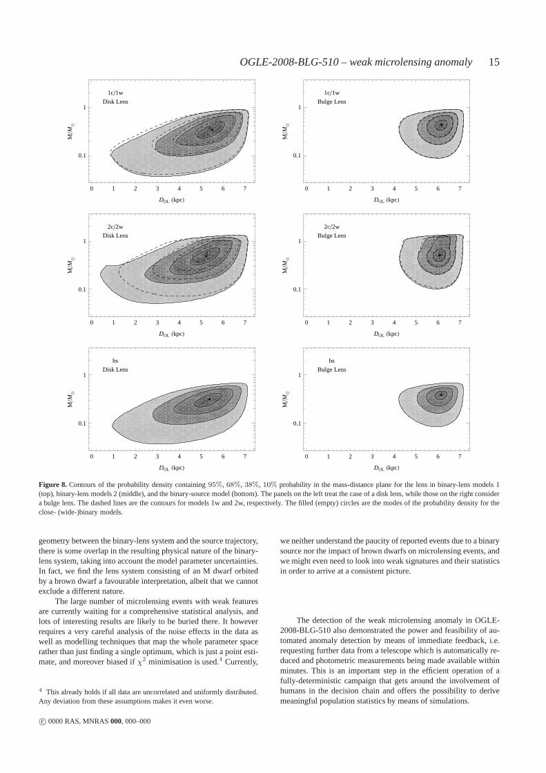
We find a probability density inDL,M , andv. By integratingover v, and changing fromM to logM , we obtain a probabilitydensity in the(DL, logM) plane. In this integration, as explainedin Dominik (2006), the dispersion in the Einstein time is practicallyirrelevant and we can approximate thetE distribution by a deltafunction. The arising posterior probabilities are illustrated in Fig.8 separately for disk and bulge lenses for models 1 and 2. We canappreciate the small difference between the close- and wide-binarymodels (whose contours are dashed in Fig. 8). The wide topologyslightly favours a smaller distance and a higher mass for thelenssystem. Higher masses are cut off by the blending constraint, as the

c© 0000 RAS, MNRAS000, 000–000

14 V. Bozza et al.

Model Prob. 〈DL〉 〈M〉 〈M1〉 〈M2〉[kpc] [M⊙] [M⊙] [Mjup]

1c Disk 46.% 4.74 0.21 0.19 281c Bulge 54.% 5.92 0.34 0.29 44

1w Disk 49.2% 4.65 0.22 0.18 421w Bulge 50.8% 5.9 0.34 0.28 64

2c Disk 53.8% 4.49 0.3 0.22 882c Bulge 46.2% 5.88 0.46 0.33 133

2w Disk 53.3% 4.66 0.36 0.23 1342w Bulge 46.7% 5.88 0.48 0.31 178

bs Disk 49.2% 4.63 0.19bs Bulge 50.8% 5.9 0.29

Table 7. Expectation values of lens distanceDL and lens massM for thedifferent binary-lens models, and assessment of probability for the lens toreside in the Galactic disk or bulge.

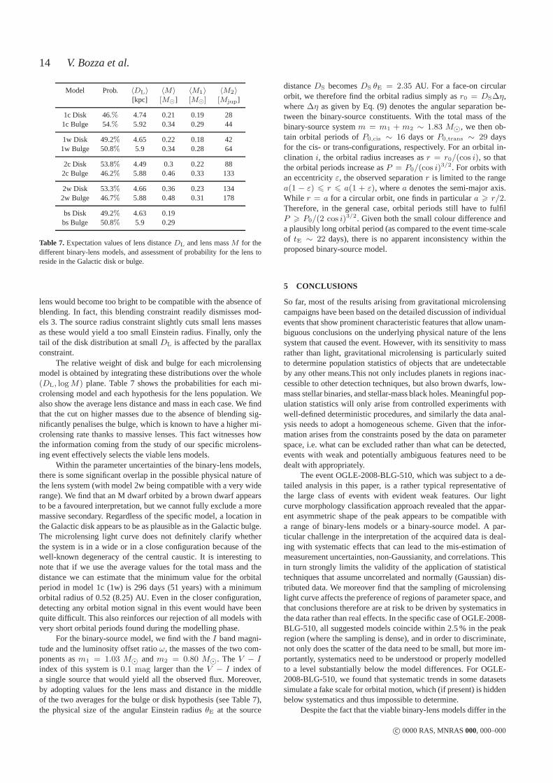
lens would become too bright to be compatible with the absence ofblending. In fact, this blending constraint readily dismisses mod-els 3. The source radius constraint slightly cuts small lensmassesas these would yield a too small Einstein radius. Finally, only thetail of the disk distribution at smallDL is affected by the parallaxconstraint.

The relative weight of disk and bulge for each microlensingmodel is obtained by integrating these distributions over the whole(DL, logM) plane. Table 7 shows the probabilities for each mi-crolensing model and each hypothesis for the lens population. Wealso show the average lens distance and mass in each case. We findthat the cut on higher masses due to the absence of blending sig-nificantly penalises the bulge, which is known to have a higher mi-crolensing rate thanks to massive lenses. This fact witnesses howthe information coming from the study of our specific microlens-ing event effectively selects the viable lens models.

Within the parameter uncertainties of the binary-lens models,there is some significant overlap in the possible physical nature ofthe lens system (with model 2w being compatible with a very widerange). We find that an M dwarf orbited by a brown dwarf appearsto be a favoured interpretation, but we cannot fully excludea moremassive secondary. Regardless of the specific model, a location inthe Galactic disk appears to be as plausible as in the Galactic bulge.The microlensing light curve does not definitely clarify whetherthe system is in a wide or in a close configuration because of thewell-known degeneracy of the central caustic. It is interesting tonote that if we use the average values for the total mass and thedistance we can estimate that the minimum value for the orbitalperiod in model 1c (1w) is 296 days (51 years) with a minimumorbital radius of 0.52 (8.25) AU. Even in the closer configuration,detecting any orbital motion signal in this event would havebeenquite difficult. This also reinforces our rejection of all models withvery short orbital periods found during the modelling phase.

For the binary-source model, we find with theI band magni-tude and the luminosity offset ratioω, the masses of the two com-ponents asm1 = 1.03 M⊙ andm2 = 0.80 M⊙. TheV − Iindex of this system is0.1 mag larger than theV − I index ofa single source that would yield all the observed flux. Moreover,by adopting values for the lens mass and distance in the middleof the two averages for the bulge or disk hypothesis (see Table 7),the physical size of the angular Einstein radiusθE at the source

distanceDS becomesDS θE = 2.35 AU. For a face-on circularorbit, we therefore find the orbital radius simply asr0 = DS∆η,where∆η as given by Eq. (9) denotes the angular separation be-tween the binary-source constituents. With the total mass of thebinary-source systemm = m1 + m2 ∼ 1.83 M⊙, we then ob-tain orbital periods ofP0,cis ∼ 16 days orP0,trans ∼ 29 daysfor the cis- or trans-configurations, respectively. For an orbital in-clination i, the orbital radius increases asr = r0/(cos i), so thatthe orbital periods increase asP = P0/(cos i)

3/2. For orbits withan eccentricityε, the observed separationr is limited to the rangea(1 − ε) 6 r 6 a(1 + ε), wherea denotes the semi-major axis.While r = a for a circular orbit, one finds in particulara > r/2.Therefore, in the general case, orbital periods still have to fulfilP > P0/(2 cos i)3/2. Given both the small colour difference anda plausibly long orbital period (as compared to the event time-scaleof tE ∼ 22 days), there is no apparent inconsistency within theproposed binary-source model.

5 CONCLUSIONS

So far, most of the results arising from gravitational microlensingcampaigns have been based on the detailed discussion of individualevents that show prominent characteristic features that allow unam-biguous conclusions on the underlying physical nature of the lenssystem that caused the event. However, with its sensitivityto massrather than light, gravitational microlensing is particularly suitedto determine population statistics of objects that are undetectableby any other means.This not only includes planets in regionsinac-cessible to other detection techniques, but also brown dwarfs, low-mass stellar binaries, and stellar-mass black holes. Meaningful pop-ulation statistics will only arise from controlled experiments withwell-defined deterministic procedures, and similarly the data anal-ysis needs to adopt a homogeneous scheme. Given that the infor-mation arises from the constraints posed by the data on parameterspace, i.e. what can be excluded rather than what can be detected,events with weak and potentially ambiguous features need tobedealt with appropriately.

The event OGLE-2008-BLG-510, which was subject to a de-tailed analysis in this paper, is a rather typical representative ofthe large class of events with evident weak features. Our lightcurve morphology classification approach revealed that theappar-ent asymmetric shape of the peak appears to be compatible witha range of binary-lens models or a binary-source model. A par-ticular challenge in the interpretation of the acquired data is deal-ing with systematic effects that can lead to the mis-estimation ofmeasurement uncertainties, non-Gaussianity, and correlations. Thisin turn strongly limits the validity of the application of statisticaltechniques that assume uncorrelated and normally (Gaussian) dis-tributed data. We moreover find that the sampling of microlensinglight curve affects the preference of regions of parameter space, andthat conclusions therefore are at risk to be driven by systematics inthe data rather than real effects. In the specific case of OGLE-2008-BLG-510, all suggested models coincide within 2.5 % in the peakregion (where the sampling is dense), and in order to discriminate,not only does the scatter of the data need to be small, but moreim-portantly, systematics need to be understood or properly modelledto a level substantially below the model differences. For OGLE-2008-BLG-510, we found that systematic trends in some datasetssimulate a fake scale for orbital motion, which (if present)is hiddenbelow systematics and thus impossible to determine.

Despite the fact that the viable binary-lens models differ in the

c© 0000 RAS, MNRAS000, 000–000

OGLE-2008-BLG-510 – weak microlensing anomaly15

1c�1w

Disk Lens

0 1 2 3 4 5 6 7

0.1

1

DOL HkpcL

M�M�

1c�1w

Bulge Lens

0 1 2 3 4 5 6 7

0.1

1

DOL HkpcL

M�M�

2c�2w

Disk Lens

0 1 2 3 4 5 6 7

0.1

1

DOL HkpcL

M�M�

2c�2w

Bulge Lens

0 1 2 3 4 5 6 7

0.1

1

DOL HkpcL

M�M�

bs

Disk Lens

0 1 2 3 4 5 6 7

0.1

1

DOL HkpcL

M�M�

bs

Bulge Lens

0 1 2 3 4 5 6 7

0.1

1

DOL HkpcL

M�M�

Figure 8. Contours of the probability density containing95%, 68%, 38%, 10% probability in the mass-distance plane for the lens in binary-lens models 1(top), binary-lens models 2 (middle), and the binary-source model (bottom). The panels on the left treat the case of a disk lens, while those on the right considera bulge lens. The dashed lines are the contours for models 1w and 2w, respectively. The filled (empty) circles are the modesof the probability density for theclose- (wide-)binary models.

geometry between the binary-lens system and the source trajectory,there is some overlap in the resulting physical nature of thebinary-lens system, taking into account the model parameter uncertainties.In fact, we find the lens system consisting of an M dwarf orbitedby a brown dwarf a favourable interpretation, albeit that wecannotexclude a different nature.

The large number of microlensing events with weak featuresare currently waiting for a comprehensive statistical analysis, andlots of interesting results are likely to be buried there. Ithoweverrequires a very careful analysis of the noise effects in the data aswell as modelling techniques that map the whole parameter spacerather than just finding a single optimum, which is just a point esti-mate, and moreover biased ifχ2 minimisation is used.4 Currently,

4 This already holds if all data are uncorrelated and uniformly distributed.Any deviation from these assumptions makes it even worse.

we neither understand the paucity of reported events due to abinarysource nor the impact of brown dwarfs on microlensing events, andwe might even need to look into weak signatures and their statisticsin order to arrive at a consistent picture.

The detection of the weak microlensing anomaly in OGLE-2008-BLG-510 also demonstrated the power and feasibility of au-tomated anomaly detection by means of immediate feedback, i.e.requesting further data from a telescope which is automatically re-duced and photometric measurements being made available withinminutes. This is an important step in the efficient operationof afully-deterministic campaign that gets around the involvement ofhumans in the decision chain and offers the possibility to derivemeaningful population statistics by means of simulations.

c© 0000 RAS, MNRAS000, 000–000

16 V. Bozza et al.

ACKNOWLEDGMENTS

The Danish 1.54m telescope is operated based on a grant from theDanish Natural Science Foundation (FNU). The “Dark Cosmol-ogy Centre” is funded by the Danish National Research Founda-tion. Work by C. Han was supported by a grant of National Re-search Foundation of Korea (2009-0081561). L. M. acknowledgessupport for this work by research funds of the InternationalInsti-tute for Advanced Scientific Studies. Work by AG was supportedby NSF grant AST-0757888. Work by BSG, AG, and RWP wassupported by NASA grant NNX08AF40G. Work by SD was per-formed under contract with the California Institute of Technology(Caltech) funded by NASA through the Sagan Fellowship Program.The MOA team acknowledges support by grants JSPS20340052,JSPS20740104 and MEXT19015005. Some of the observations re-ported in this paper were obtained with the Southern AfricanLargeTelescope (SALT). LM acknowledges support for this work by re-search funds of the International Institute for Advanced ScientificStudies. MH acknowledges support by the German Research Foun-dation (DFG). DR (boursier FRIA) and JSurdej acknowledge sup-port from the Communaute francaise de Belgique – Actions derecherche concertees – Academie universitaire Wallonie-Europe.The OGLE project has received funding from the European Re-search Council under the European Community’s Seventh Frame-work Programme (FP7/2007-2013) / ERC grant agreement no.246678. MD, YT, DMB, CL, MH, RAS, KH, and CS are thank-ful to Qatar National Research Fund (QNRF), member of QatarFoundation, for support by grant NPRP 09-476-1-078.

REFERENCES

Afonso C., et al., 2003, A&A, 404, 145Alard C., Lupton R. H., 1998, ApJ, 503, 325Albrow M., et al., 1998, ApJ, 509, 687Albrow M. D., 2004, ApJ, 607, 821Albrow M. D., et al., 1999, ApJ, 522, 1022Alcock C., et al., 1996, ApJ, 463, L67Alcock C., et al., 1997, ApJ, 479, 119Ansari R., 1994, Une methode de reconstruction photometriquepour l’experience EROS, preprint LAL 94-10

Beaulieu J.-P., et al., 2006, Nature, 439, 437Bennett D. P., Rhie S. H., 2002, ApJ, 574, 985Bensby T., et al., 2011, A&A, 533, A134Bessell M. S., Brett J. M., 1988, PASP, 100, 1134Bond I. A., et al., 2001, MNRAS, 327, 868Bozza V., 2001, A&A, 374, 13Bozza V., 2010, MNRAS, 408, 2188Bramich D. M., 2008, MNRAS, 386, L77Bramich D. M., et al., 2011, MNRAS, 413, 1275Burgdorf M. J., Bramich D. M., Dominik M., Bode M. F., HorneK. D., Steele I. A., Rattenbury N., Tsapras Y., 2007, P&SS, 55,582

Calchi Novati S., de Luca F., Jetzer P., Mancini L., Scarpetta G.,2008, A&A, 480, 723

Cassan A., 2008, A&A, 491, 587Cassan A., et al., 2011, Nature acceptedChabrier G., 2003, PASP, 115, 763Choi J.-Y., et al., 2011, Characterization of Lenses and LensedStars from Extremely High-Magnification Events, to be submit-ted to ApJ

Dominik M., 1995, A&AS, 109, 597

Dominik M., 1998a, A&A, 333, L79Dominik M., 1998b, A&A, 333, 893Dominik M., 1999a, A&A, 341, 943Dominik M., 1999b, A&A, 349, 108Dominik M., 2006, MNRAS, 367, 669Dominik M., 2010, General Relativity and Gravitation, 42, 2075Dominik M., 2011, MNRAS, 411, 2Dominik M., et al., 2002, P&SS, 50, 299Dominik M., et al., 2007, MNRAS, 380, 792Dominik M., et al., 2008a, in Y.-S. Sun, S. Ferraz-Mello, &J.-L. Zhou ed., IAU Symposium Vol. 249 of IAU Sympo-sium, ARTEMiS (Automated Robotic Terrestrial Exoplanet Mi-crolensing Search) – Hunting for planets of Earth mass and be-low. pp 35–41

Dominik M., et al., 2008b, AN, 329, 248Dominik M., et al., 2010, AN, 331, 671Dominik M., Hirshfeld A. C., 1996, A&A, 313, 841Einstein A., 1936, Science, 84, 506Erdl H., Schneider P., 1993, A&A, 268, 453Fried D. L., 1978, JOSA, 68, 1651Gaudi B. S., 1998, ApJ, 506, 533Gaudi B. S., Han C., 2004, ApJ, 611, 528Gould A., 2004, ApJ, 606, 319Gould A., et al., 2010, ApJ, 720, 1073Gould A., Gaucherel C., 1997, ApJ, 477, 580Gould A., Loeb A., 1992, ApJ, 396, 104Grenacher L., Jetzer P., Strassle M., de Paolis F., 1999, A&A, 351,775

Griest K., Hu W., 1992, ApJ, 397, 362Griest K., Safizadeh N., 1998, ApJ, 500, 37Grundahl F., Christensen-Dalsgaard J., Arentoft T., Frandsen S.,Kjeldsen H., Jørgensen U. G., Kjærgaard P., 2009, Communica-tions in Asteroseismology, 158, 345

Han C., 2007, ApJ, 661, 1202Han C., et al., 2009, ApJ, 705, 1116Han C., Gould A., 1995, ApJ, 449, 521Han C., Jeong Y., 1998, MNRAS, 301, 231Horne K., Snodgrass C., Tsapras Y., 2009, MNRAS, 396, 2087Jaroszynski M., Paczynski B., 2002, AcA, 52, 361Jørgensen U. G., 2008, Physica Scripta, T130, 014008Kains N., et al., 2009, MNRAS, 395, 787Kervella P., Bersier D., Mourard D., Nardetto N., Fouque P.,Coude du Foresto V., 2004, A&A, 428, 587

Kiraga M., Paczynski B., 1994, ApJ, 430, L101Mao S., Di Stefano R., 1995, ApJ, 440, 22Mao S., Paczynski B., 1991, ApJ, 374, L37Muraki Y., et al., 2011, ApJ, 741, 22Night C., Di Stefano R., Schwamb M., 2008, ApJ, 686, 785Paczynski B., 1986, ApJ, 304, 1Paczynski B., 1991, ApJ, 371, L63Paczynski B., 1996, ARA&A, 34, 419Sumi T., et al., 2010, ApJ, 710, 1641Tsapras Y., et al., 2009, AN, 330, 4Tubbs R. N., Baldwin J. E., Mackay C. D., Cox G. C., 2002, A&A,387, L21

Udalski A., 2003, AcA, 53, 291Udalski A., Szymanski M., Kałuzny J., Kubiak M., Mateo M.,1992, AcA, 42, 253

Udalski A., Szymanski M., Kałuzny J., Kubiak M., Mateo M.,Krzeminski W., Paczynski B., 1994, AcA, 44, 227

Yoo J., et al., 2004, ApJ, 616, 1204

c© 0000 RAS, MNRAS000, 000–000

OGLE-2008-BLG-510 – weak microlensing anomaly17

(Affiliations continued)

21South African Large Telescope, P.O. Box 9 Observatory 7935,South Africa22Department of Physics and Astrophysics, Faculty of Science, Nagoya University, Nagoya 464-8602, Japan23Armagh Observatory, College Hill, Armagh, BT61 9DG, Northern Ireland, United Kingdom24Korea Astronomy and Space Science Institute, 776 Daedukdae-ro, Yuseong-gu, Daejeon 305-348, Republic of Korea25Istituto Internazionale per gli Alti Studi Scientifici (IIASS), Vietri Sul Mare (SA), Italy26Max Planck Institute for Astronomy, Konigstuhl 17, 619117Heidelberg, Germany27INFN, Gruppo Collegato di Salerno, Sezione di Napoli, Italy28Centro de Astro-Ingenierıa, Departamento de Astronomıay Astrofısica, Pontificia Universidad Catolica de Chile,Casilla 306, Santiago, Chile29Deutsches SOFIA Institut, Universitat Stuttgart, Pfaffenwaldring 31, 70569 Stuttgart, Germany30SOFIA Science Center, NASA Ames Research Center, Mail Stop N211-3, Moffett Field CA 94035, United States of America31Danmarks Tekniske Universitet, Institut for Rumforskningog -teknologi, Juliane Maries Vej 30, 2100 Kbenhavn, Denmark32Bellatrix Astronomical Observatory, Via Madonna de Loco 47, 03023 Ceccano (FR), Italy33Department of Physics, Sharif University of Technology, P.O. Box 11155–9161, Tehran, Iran34Institut d’Astrophysique et de Geophysique, Allee du 6 Aout 17, Sart Tilman, Bat. B5c, 4000 Liege, Belgium35European Southern Observatory (ESO) Alonso de Cordova 3107, Casilla 19001, Santiago 19, Chile36Max Planck Institute for Solar System Research, Max-Planck-Str. 2, 37191 Katlenburg-Lindau, Germany37Astrophysics Group, Keele University, Staffordshire, ST55BG, United Kingdom38Astrophysics Research Institute, Liverpool John Moores University, Twelve Quays House, Egerton Wharf, Birkenhead CH41 1LD, United Kingdom39Instituto de Astrofısica de Andalucıa, Glorieta de la Astronomıa s/n, 18008 Granada, Spain40Dark Cosmology Centre, Niels Bohr Institutet, Københavns Universitet, Juliane Maries Vej 30, 2100 København Ø, Denmark41University of Canterbury, Department of Physics and Astronomy, Private Bag 4800, Christchurch 8020, New Zealand42Department of Physics, 225 Nieuwland Science Hall, University of Notre Dame, Notre Dame, IN 46556, United States of America43McDonald Observatory, 16120 St Hwy Spur 78 #2, Fort Davis, TX79734, United States of America44University of Tasmania, School of Mathematics and Physics,Private Bag 37, Hobart, TAS 7001, Australia45Institute of Geophysics and Planetary Physics (IGPP), L-413, Lawrence Livermore National Laboratory, PO Box 808, Livermore, CA 94551, United Statesof America46Department of Physics, University of Rijeka, Omladinska 14, 51000 Rijeka, Croatia47Technische Universitat Wien, Wiedner Hauptstr. 8-10, 1040 Wien, Austria48NASA Exoplanet Science Institute, Caltech, MS 100-22, 770 South Wilson Avenue, Pasadena, CA 91125, United States of America49Perth Observatory, Walnut Road, Bickley, Perth 6076, WA, Australia50South African Astronomical Observatory, P.O. Box 9 Observatory 7935, South Africa51Space Telescope Science Institute, 3700 San Martin Drive, Baltimore, MD 21218, United States of America52Universidad de Concepcion, Departamento de Astronomia, Casilla 160–C, Concepcion, Chile53Department of Physics, Texas A&M University, 4242 TAMU, College Station, TX 77843-4242, United States of America54Institute for Advanced Study, Einstein Drive, Princeton, NJ 08540, United States of America55Department of Physics, Ohio State University, 191 W. Woodruff, Columbus, OH 43210, United States of America56Mt. John Observatory, P.O. Box 56, Lake Tekapo 8770, New Zealand57School of Chemical and Physical Sciences, Victoria University, Wellington, New Zealand58Department of Physics, Konan University, Nishiokamoto 8-9-1, Kobe 658-8501, Japan59Nagano National College of Technology, Nagano 381-8550, Japan60Tokyo Metropolitan College of Aeronautics, Tokyo 116-8523, Japan61Department of Earth and Space Science, Osaka University, 1-1 Machikaneyama-cho, Toyonaka, Osaka 560-0043, Japan62Department of Earth Sciences, National Taiwan Normal University, No. 88, Section 4, Tingzhou Road, Wenshan District, Taipei 11677, Taiwan

c© 0000 RAS, MNRAS000, 000–000