Embed Size (px)
Citation preview
Subsurface Sources of CO2 in the Contiguous United States
Volume 1: Discovered Reservoirs March 5, 2014 DOE/NETL-2014/1637
Working Paper
OFFICE OF FOSSIL ENERGY
National Energy Technology Laboratory

Subsurface Sources of CO2 in the Contiguous United States
Disclaimer
This report was prepared as an account of work sponsored by an agency of the United States Government. Neither the United States Government nor any agency thereof, nor any of their employees, makes any warranty, express or implied, or assumes any legal liability or responsibility for the accuracy, completeness, or usefulness of any information, apparatus, product, or process disclosed, or represents that its use would not infringe privately owned rights. Reference therein to any specific commercial product, process, or service by trade name, trademark, manufacturer, or otherwise does not necessarily constitute or imply its endorsement, recommendation, or favoring by the United States Government or any agency thereof. The views and opinions of authors expressed therein do not necessarily state or reflect those of the United States Government or any agency thereof.
All exhibits have been created by Enegis, LLC, unless otherwise noted.

Subsurface Sources of CO2 in the Contiguous United States
Author List:
Energy Sector Planning and Analysis (ESPA)
Jeffrey Eppink, RG, RGph, MBA, Tom L. Heidrick, Ramon Alvarado, Michael Marquis
Enegis, LLC
National Energy Technology Laboratory (NETL)
Phil DiPietro Strategic Energy Analysis and Planning Division
Contributor:
Robert Wallace Booz Allen Hamilton, Inc.
This report was prepared by Energy Sector Planning and Analysis (ESPA) for the United States Department of Energy (DOE), National Energy Technology Laboratory (NETL). This work was completed under DOE NETL Contract Number DE-FE0004001. This work was performed under ESPA Task 150.07.05.
The authors wish to acknowledge the excellent guidance, contributions, and cooperation of the NETL staff, particularly:
Ms. Evelyn Dale Dr. David Morgan
Dr. Angela Goodman Dr. Brian Strazisar
DOE Contract Number DE-FE0004001

Subsurface Sources of CO2 in the Contiguous United States
This page intentionally left blank.
Subsurface Sources of CO2 in the Contiguous United States
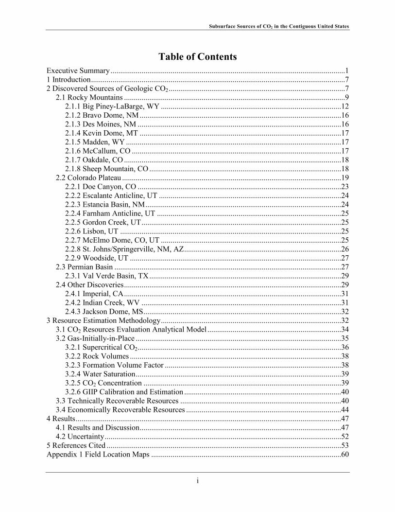
Table of Contents Executive Summary .........................................................................................................................1 1 Introduction ...................................................................................................................................7 2 Discovered Sources of Geologic CO2 ...........................................................................................7
2.1 Rocky Mountains ..................................................................................................................9 2.1.1 Big Piney-LaBarge, WY .............................................................................................12 2.1.2 Bravo Dome, NM ........................................................................................................16 2.1.3 Des Moines, NM .........................................................................................................16 2.1.4 Kevin Dome, MT ........................................................................................................17 2.1.5 Madden, WY ...............................................................................................................17 2.1.6 McCallum, CO ............................................................................................................17 2.1.7 Oakdale, CO ................................................................................................................18 2.1.8 Sheep Mountain, CO ...................................................................................................18
2.2 Colorado Plateau .................................................................................................................19 2.2.1 Doe Canyon, CO .........................................................................................................23 2.2.2 Escalante Anticline, UT ..............................................................................................24 2.2.3 Estancia Basin, NM .....................................................................................................24 2.2.4 Farnham Anticline, UT ...............................................................................................25 2.2.5 Gordon Creek, UT .......................................................................................................25 2.2.6 Lisbon, UT ..................................................................................................................25 2.2.7 McElmo Dome, CO, UT .............................................................................................25 2.2.8 St. Johns/Springerville, NM, AZ .................................................................................26 2.2.9 Woodside, UT .............................................................................................................27
2.3 Permian Basin .....................................................................................................................27 2.3.1 Val Verde Basin, TX ...................................................................................................29
2.4 Other Discoveries ................................................................................................................29 2.4.1 Imperial, CA ................................................................................................................31 2.4.2 Indian Creek, WV .......................................................................................................31 2.4.3 Jackson Dome, MS ......................................................................................................32
3 Resource Estimation Methodology .............................................................................................32 3.1 CO2 Resources Evaluation Analytical Model .....................................................................34 3.2 Gas-Initially-in-Place ..........................................................................................................35
3.2.1 Supercritical CO2 .........................................................................................................36 3.2.2 Rock Volumes .............................................................................................................38 3.2.3 Formation Volume Factor ...........................................................................................38 3.2.4 Water Saturation ..........................................................................................................39 3.2.5 CO2 Concentration ......................................................................................................39 3.2.6 GIIP Calibration and Estimation .................................................................................40
3.3 Technically Recoverable Resources ...................................................................................40 3.4 Economically Recoverable Resources ................................................................................44
4 Results .........................................................................................................................................47 4.1 Results and Discussion ........................................................................................................47 4.2 Uncertainty ..........................................................................................................................52
5 References Cited .........................................................................................................................53 Appendix 1 Field Location Maps ..................................................................................................60
i

Subsurface Sources of CO2 in the Contiguous United States
Appendix 2 Disaggregated Field Parameters and Results from CREAM .....................................80
ii
Subsurface Sources of CO2 in the Contiguous United States
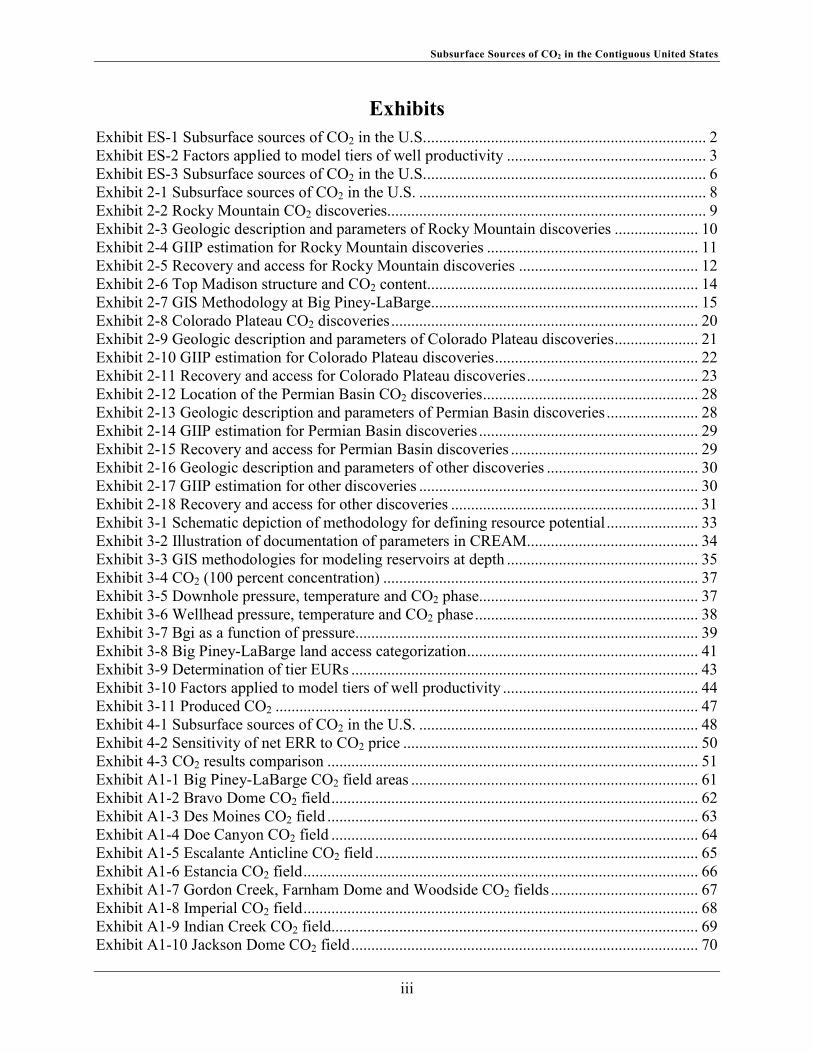
Exhibits Exhibit ES-1 Subsurface sources of CO2 in the U.S. ...................................................................... 2 Exhibit ES-2 Factors applied to model tiers of well productivity .................................................. 3 Exhibit ES-3 Subsurface sources of CO2 in the U.S. ...................................................................... 6 Exhibit 2-1 Subsurface sources of CO2 in the U.S. ........................................................................ 8 Exhibit 2-2 Rocky Mountain CO2 discoveries................................................................................ 9 Exhibit 2-3 Geologic description and parameters of Rocky Mountain discoveries ..................... 10 Exhibit 2-4 GIIP estimation for Rocky Mountain discoveries ..................................................... 11 Exhibit 2-5 Recovery and access for Rocky Mountain discoveries ............................................. 12 Exhibit 2-6 Top Madison structure and CO2 content.................................................................... 14 Exhibit 2-7 GIS Methodology at Big Piney-LaBarge................................................................... 15 Exhibit 2-8 Colorado Plateau CO2 discoveries ............................................................................. 20 Exhibit 2-9 Geologic description and parameters of Colorado Plateau discoveries ..................... 21 Exhibit 2-10 GIIP estimation for Colorado Plateau discoveries ................................................... 22 Exhibit 2-11 Recovery and access for Colorado Plateau discoveries ........................................... 23 Exhibit 2-12 Location of the Permian Basin CO2 discoveries ...................................................... 28 Exhibit 2-13 Geologic description and parameters of Permian Basin discoveries ....................... 28 Exhibit 2-14 GIIP estimation for Permian Basin discoveries ....................................................... 29 Exhibit 2-15 Recovery and access for Permian Basin discoveries ............................................... 29 Exhibit 2-16 Geologic description and parameters of other discoveries ...................................... 30 Exhibit 2-17 GIIP estimation for other discoveries ...................................................................... 30 Exhibit 2-18 Recovery and access for other discoveries .............................................................. 31 Exhibit 3-1 Schematic depiction of methodology for defining resource potential ....................... 33 Exhibit 3-2 Illustration of documentation of parameters in CREAM........................................... 34 Exhibit 3-3 GIS methodologies for modeling reservoirs at depth ................................................ 35 Exhibit 3-4 CO2 (100 percent concentration) ............................................................................... 37 Exhibit 3-5 Downhole pressure, temperature and CO2 phase....................................................... 37 Exhibit 3-6 Wellhead pressure, temperature and CO2 phase ........................................................ 38 Exhibit 3-7 Bgi as a function of pressure...................................................................................... 39 Exhibit 3-8 Big Piney-LaBarge land access categorization .......................................................... 41 Exhibit 3-9 Determination of tier EURs ....................................................................................... 43 Exhibit 3-10 Factors applied to model tiers of well productivity ................................................. 44 Exhibit 3-11 Produced CO2 .......................................................................................................... 47 Exhibit 4-1 Subsurface sources of CO2 in the U.S. ...................................................................... 48 Exhibit 4-2 Sensitivity of net ERR to CO2 price .......................................................................... 50 Exhibit 4-3 CO2 results comparison ............................................................................................. 51 Exhibit A1-1 Big Piney-LaBarge CO2 field areas ........................................................................ 61 Exhibit A1-2 Bravo Dome CO2 field ............................................................................................ 62 Exhibit A1-3 Des Moines CO2 field ............................................................................................. 63 Exhibit A1-4 Doe Canyon CO2 field ............................................................................................ 64 Exhibit A1-5 Escalante Anticline CO2 field ................................................................................. 65 Exhibit A1-6 Estancia CO2 field ................................................................................................... 66 Exhibit A1-7 Gordon Creek, Farnham Dome and Woodside CO2 fields ..................................... 67 Exhibit A1-8 Imperial CO2 field ................................................................................................... 68 Exhibit A1-9 Indian Creek CO2 field............................................................................................ 69 Exhibit A1-10 Jackson Dome CO2 field ....................................................................................... 70
iii
Subsurface Sources of CO2 in the Contiguous United States
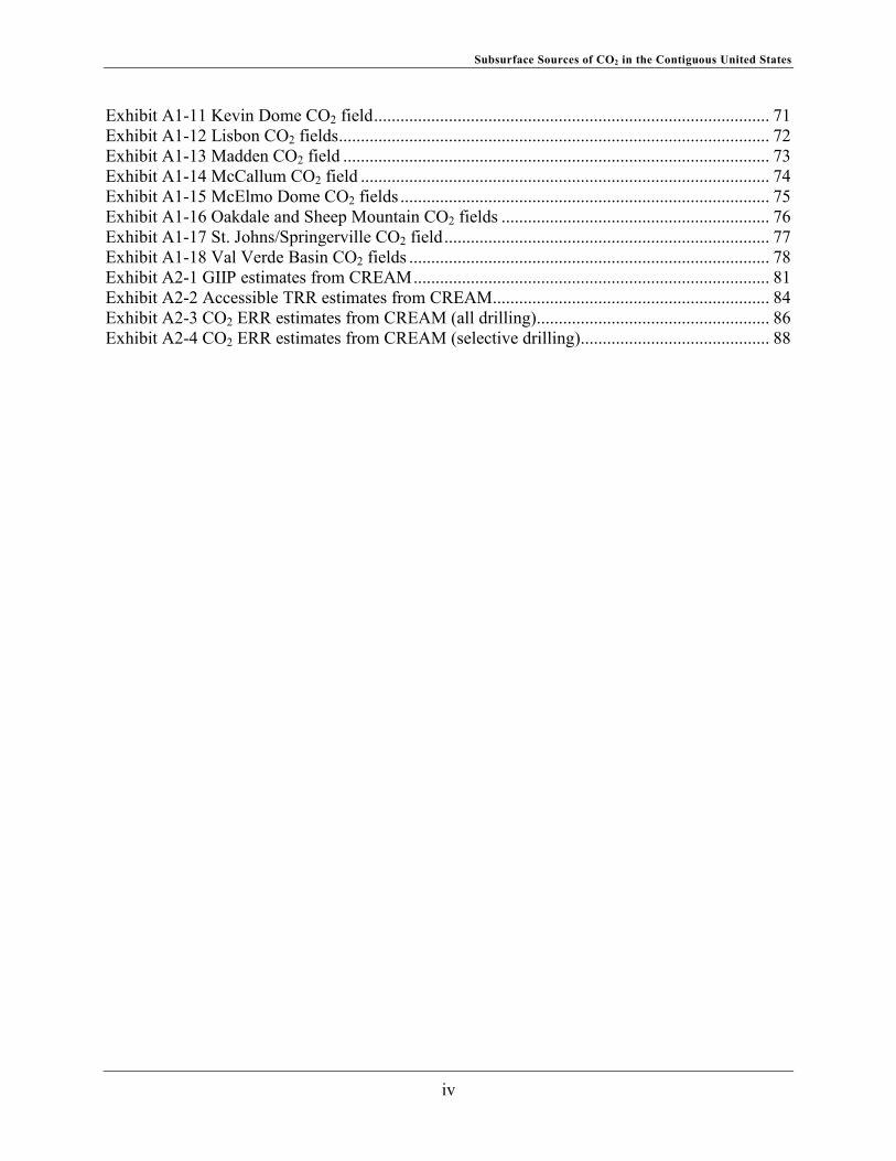
Exhibit A1-11 Kevin Dome CO2 field .......................................................................................... 71 Exhibit A1-12 Lisbon CO2 fields .................................................................................................. 72 Exhibit A1-13 Madden CO2 field ................................................................................................. 73 Exhibit A1-14 McCallum CO2 field ............................................................................................. 74 Exhibit A1-15 McElmo Dome CO2 fields .................................................................................... 75 Exhibit A1-16 Oakdale and Sheep Mountain CO2 fields ............................................................. 76 Exhibit A1-17 St. Johns/Springerville CO2 field .......................................................................... 77 Exhibit A1-18 Val Verde Basin CO2 fields .................................................................................. 78 Exhibit A2-1 GIIP estimates from CREAM ................................................................................. 81 Exhibit A2-2 Accessible TRR estimates from CREAM ............................................................... 84 Exhibit A2-3 CO2 ERR estimates from CREAM (all drilling)..................................................... 86 Exhibit A2-4 CO2 ERR estimates from CREAM (selective drilling)........................................... 88
iv

Subsurface Sources of CO2 in the Contiguous United States
Acronyms and Abbreviations 3P Proven, probable and possible AF Access factor AU Assessment Unit Bcf Billion cubic feet Bcfd Billion cubic feet per day Bgi Formation volume factor BLM Bureau of Land Management BPLB Big Piney-LaBarge field CAPEX Capital expense CO2 Carbon dioxide CREAM CO2 Resources Evaluation
Analytical Model DOE Department of Energy EBT Earnings before taxes EIA Energy Information Administration EOR Enhanced oil recovery EPA Environmental Protection Agency ERR Economically recoverable
resources ESPA Energy Sector Planning and
Analysis ETSAP Energy Technology Systems
Analysis Programme EUR Estimated ultimate recovery GIIP Gas-initially-in-place GIS Geographical Information System IEA International Energy Agency INGAA Interstate Natural Gas Association
of America
Ma Millions of years ago Mcf Thousand cubic feet mD Millidarcy MGS Montana Geological Society MMcf Million cubic feet MMcfd Million cubic feet per day
_ Natural gas EUR for a specific tier NETL National Energy Technology
Laboratory NPV Net present value OPEX Operating expense ppm Parts per million psi Pounds per square inch rcf Reservoir cubic feet RF Recovery factor scf Standard cubic feet SEC Securities and Exchange
Commission SMU Southern Methodist University T Tier TI Tier (inclusive) Tcf Trillion cubic feet TRR Technically recoverable resources UGS Utah Geological Survey U.S. United States USGS U.S. Geological Survey VBA Visual Basic for Applications
v

Subsurface Sources of CO2 in the Contiguous United States
This page intentionally left blank.
vi

Subsurface Sources of CO2 in the Contiguous United States
Executive Summary The production of carbon dioxide (CO2) from subsurface sources in the United States has grown from 0.6 Tcf per year in 2000 to 1.1 Tcf per year in 2013. Approximately 97 percent of the CO2 is used for enhanced oil recovery (EOR). In response to continued and growing demand in this sector, production has recently been initiated at Doe Canyon and, with the exception of Sheep Mountain which is in decline, all established CO2 production operations are undergoing drilling programs or expansions of gas processing facilities to increase the rate of production. Production from subsurface sources of CO2 is forecast to reach 1.5 Tcf/yr by 2018. (Murrell, 2013)
This study compiles information about subsurface carbon dioxide (CO2) accumulations in the continental United States and estimates the recoverable resource. Twenty-one CO2 fields in the contiguous states contain an estimated 311 Tcf of CO2 gas-initially-in-place (GIIP). Of that, 168 Tcf (54 percent) is estimated to be accessible and technically recoverable. The estimated economically recoverable resource (ERR) is 96.4 Tcf, based on a CO2 price of 1.06 $/mcf ($20/tonne) at the field gate. Cumulative production to date is 18.9 Tcf, leaving 77.5 Tcf remaining or net ERR. The Big Piney-LaBarge field in Wyoming contains an estimated net ERR of 52 Tcf, 67 percent of the total for the United States. The remaining ERR in reservoirs that feed into the Permian Basin and Gulf Coast is on the order of 10-20 years of supply. The technically recoverable resource (TRR) in the Permian Basin and Gulf Coast is on the order of 30 years of supply. The ERR at LaBarge contains an estimated 260 Bcf of helium, while the ERR at St Johns/Springerville may contain 25 Bcf of helium.
Exhibit ES-1 shows the location of the twenty-one CO2 fields. Three adjoining states, Colorado, Wyoming and Utah, account for 71 percent of the GIIP. Pipeline infrastructure connects many of the CO2 fields in Colorado and Utah to the oil fields in the Permian basin. Newly built pipelines are enabling increased utilization of the CO2 resources in Wyoming and Mississippi.
Data was gathered from technical journals and other sources to enable the volumetric calculation for GIIP. The volumetric calculation was tailored to the resolution of the data available for each CO2 field. For Big Piney LaBarge, we employed GIS methods to integrate data from maps showing structural depth and CO2 concentration contours and identified 48 polygons with unique combinations of these attributes. We report Val Verde as one source, but technically it is seven distinct fields producing from seven distinct reservoirs, two in the upper plate of the Marathon Thrust and five in the Marathon subthrust. Escalante comprises five vertically stacked reservoirs within the same field. Similarly, Kevin and Gordon Creek are both single fields with two vertically-stacked reservoirs. In the case of stacked reservoirs, wells were modeled with multiple completions. The other sixteen fields are modeled as horizontal disks with a single-point estimate for depth, porosity, etc.
1

Subsurface Sources of CO2 in the Contiguous United States
Exhibit ES-1 Subsurface sources of CO2 in the U.S.
2
Subsurface Sources of CO2 in the Contiguous United States
Two degradations were applied to GIIP to estimate TRR. First, reservoir maps were overlain with GIS shape files for national parks, historical sites, wetlands and other areas where drilling is restricted, then the percent of accessible reservoir area was estimated. Second, the percent of accessible GIIP that could be technically produced was estimated. An expected recovery factor of 70 percent GIIP was used as a baseline, as is typical for natural gas and confirmed by studies of CO2 reservoirs previously conducted by the authors. This baseline recovery factor was adjusted up or down for each reservoir based on its geology.
A project cash flow model was exercised to make the ERR determinations for each field. The revenues from produced CO2 and other by-products and contaminants (helium, methane, nitrogen, etc.) were matched against the cost of drilling wells and also the cost of processing and compressing the produced gas. A 12 percent discount rate (after tax) was used.
The economics of the subsurface sources is primarily influenced by the estimated ultimate recovery (EUR) per well, which in our characterization is a function of the density of the resource (Bcf CO2 per acre). Thicker pay and higher porosity improve the density, all else equal. If the reservoir temperature and pressure are such that CO2 exists in the formation as a supercritical fluid (as opposed to a gas) the density is significantly higher. CO2 is supercritical in all of the formations except Bravo and St. Johns. Escalante and Kevin Dome are within the supercritical region but are borderline. The best reservoirs (top third of GIIP) have a resource density of 0.30 – 0.35 BscfCO2/acre. The middle third of GIIP has a density between 0.15 and 0.3 Bscf CO2/acre.
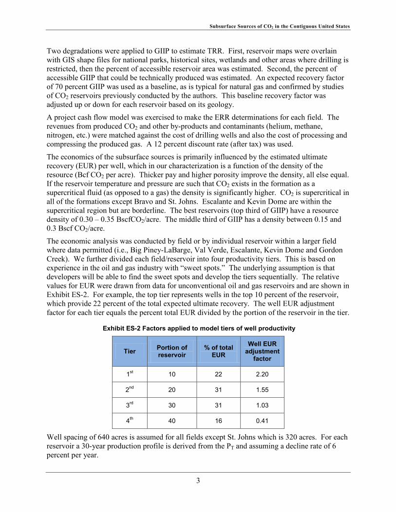
The economic analysis was conducted by field or by individual reservoir within a larger field where data permitted (i.e., Big Piney-LaBarge, Val Verde, Escalante, Kevin Dome and Gordon Creek). We further divided each field/reservoir into four productivity tiers. This is based on experience in the oil and gas industry with “sweet spots.” The underlying assumption is that developers will be able to find the sweet spots and develop the tiers sequentially. The relative values for EUR were drawn from data for unconventional oil and gas reservoirs and are shown in Exhibit ES-2. For example, the top tier represents wells in the top 10 percent of the reservoir, which provide 22 percent of the total expected ultimate recovery. The well EUR adjustment factor for each tier equals the percent total EUR divided by the portion of the reservoir in the tier.
Exhibit ES-2 Factors applied to model tiers of well productivity
Tier Portion of reservoir
% of total EUR
Well EUR adjustment
factor
1st 10 22 2.20
2nd 20 31 1.55
3rd 30 31 1.03
4th 40 16 0.41
Well spacing of 640 acres is assumed for all fields except St. Johns which is 320 acres. For each reservoir a 30-year production profile is derived from the PT and assuming a decline rate of 6 percent per year.
3
Subsurface Sources of CO2 in the Contiguous United States
The cash flow model assumes an average cost of $630/ft for each production well (U.S. DOE Energy Information Administration) with some regional adjustments and a 15 percent dry hole burden. The compressor cost factor is 0.237 $/MMcf/delta psi (draft NETL report). The required pressure gain is a function of the well head pressure (calculated from the downhole pressure and an estimated well bore gradient, gathering line losses and the estimated pressure drop across gas processing equipment).
The assumed selling price for CO2 is 1.06 $/Mcf ($20/tonne) at pipeline purity and pressure at the field gate. If nitrogen in the produced gas is above 4 percent we assume it must be separated out, which represents a significant expense. We assume that hydrogen sulfide (H2S), methane and light hydrocarbons can be separated and sold. If helium is present at a concentration above 0.3 vol% (Big Piney LaBarge and St. Johns) we assume it can be captured and sold. We use 125 $/Mscf as the long-term price for helium.
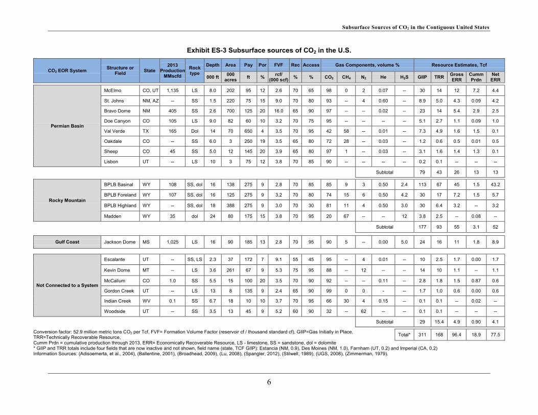
Exhibit ES-3 presents a one-page overview of the analysis. For each CO2 field the production rate during 2013 is shown, as are key parameters that support the GIIP and TRR calculations, the latter of which is derived from the GIIP and the access and technical recovery degradation factors. The exhibit also shows the average gas composition at each field. For fields that were divided into reservoirs or polygons, Exhibit ES-3 presents weighted average values for the field overall. Big Piney LaBarge is divided into three areas, basinal, foreland and highland based on topographic expression, to represent differences in accessibility and drill depth. The overall observation from Exhibit ES-3 is that each CO2 field offers a unique combination of size, resource density, accessibility and produced gas composition that affect the economics of production.
This analysis was conducted without consideration of markets or capital investment requirements beyond the field lease line at each of the CO2 fields. The ERR calculation would be different if one took into consideration, for example, existing CO2 compression or pipeline transport infrastructure at Val Verde. In that way, the ERR analysis is designed to offer a comparison of the quality of the different fields/reservoirs. Exhibit ES-3 shows both the “gross ERR” and the “net ERR.” The gross ERR for a field equals the sum of the potential production from all the reservoir-tiers that clear economic criteria. The net ERR equals the gross ERR minus the cumulative amount of CO2 already produced from that field.
We exercised the cash flow model to estimate the sensitivity of the results to the assumed price of CO2. Decreasing the price 25 percent to 0.8 $/Mscf (15 $/mtCO2) causes a 73 percent reduction in net ERR, from 77.5 Tcf to 21 Tcf. Increasing the CO2 price 25 percent to 1.32 $/Mscf (25 $/mtCO2) increases the ERR 35 percent to 105 Tcf.
There are other areas of uncertainty in the estimates for GIIP, TRR and ERR. For example, we were not able to find unique maps for Bravo or Jackson Dome. The cost and performance of helium capture systems and other gas processing operations are held as proprietary. We do not have production well models or systems analyses of gas processing systems to predict CO2 compressor inlet pressure at each field. The TRR recovery factors (%GIIP recoverable) are based on literature research and the expertise of the authors rather than measurements of reservoir permeability. Well spacing is generically applied. NETL is undertaking efforts to address these areas of uncertainty and others and plans to publish an updated version of its working paper.
4

Subsurface Sources of CO2 in the Contiguous United States
Another source of uncertainty in the resource estimate is the potential for discovery of new CO2 field(s). Accordingly, NETL is undertaking a parallel effort to identify and assess leads for undiscovered CO2 resources in the United States. That study looks more closely at the geology and tectonics of the discovered CO2 reservoirs and the sequence of trap formation and CO2 emplacement. The study then explores five areas for possible undiscovered leads within the geologic trends where the discovered reservoirs are found. A companion NETL document contains the analysis of undiscovered CO2 resources.
5
Subsurface Sources of CO2 in the Contiguous United States
Exhibit ES-3 Subsurface sources of CO2 in the U.S.
CO2 EOR System Structure or Field State
2013 Production
MMscfd
Rock type
Depth Area Pay Por FVF Rec Access Gas Components, volume % Resource Estimates, Tcf
000 ft 000 acres ft % rcf/
(000 scf) % % CO2 CH4 N2 He H2S GIIP TRR Gross ERR
Cumm Prdn
Net ERR
Permian Basin
McElmo CO, UT 1,135 LS 8.0 202 95 12 2.6 70 65 98 0 2 0.07 -- 30 14 12 7.2 4.4
St. Johns NM, AZ -- SS 1.5 220 75 15 9.0 70 80 93 -- 4 0.60 -- 8.9 5.0 4.3 0.09 4.2
Bravo Dome NM 405 SS 2.6 700 125 20 16.0 65 90 97 -- -- 0.02 -- 23 14 5.4 2.9 2.5
Doe Canyon CO 105 LS 9.0 82 60 10 3.2 70 75 95 -- -- -- -- 5.1 2.7 1.1 0.09 1.0
Val Verde TX 165 Dol 14 70 650 4 3.5 70 95 42 58 -- 0.01 -- 7.3 4.9 1.6 1.5 0.1
Oakdale CO -- SS 6.0 3 250 19 3.5 65 80 72 28 -- 0.03 -- 1.2 0.6 0.5 0.01 0.5
Sheep CO 45 SS 5.0 12 145 20 3.9 65 80 97 1 -- 0.03 -- 3.1 1.6 1.4 1.3 0.1
Lisbon UT -- LS 10 3 75 12 3.8 70 85 90 -- -- -- -- 0.2 0.1 -- -- --
Subtotal 79 43 26 13 13
Rocky Mountain
BPLB Basinal WY 108 SS, dol 16 138 275 9 2.8 70 85 85 9 3 0.50 2.4 113 67 45 1.5 43.2
BPLB Foreland WY 107 SS, dol 16 125 275 9 3.2 70 80 74 15 6 0.50 4.2 30 17 7.2 1.5 5.7
BPLB Highland WY -- SS, dol 18 388 275 9 3.0 70 30 81 11 4 0.50 3.0 30 6.4 3.2 -- 3.2
Madden WY 35 dol 24 80 175 15 3.8 70 95 20 67 -- -- 12 3.8 2.5 -- 0.08 --
Subtotal 177 93 55 3.1 52
Gulf Coast Jackson Dome MS 1,025 LS 16 90 185 13 2.8 70 95 90 5 -- 0.00 5.0 24 16 11 1.8 8.9
Not Connected to a System
Escalante UT -- SS, LS 2.3 37 172 7 9.1 55 45 95 -- 4 0.01 -- 10 2.5 1.7 0.00 1.7
Kevin Dome MT -- LS 3.6 261 67 9 5.3 75 95 88 -- 12 -- -- 14 10 1.1 -- 1.1
McCallum CO 1.0 SS 5.5 15 100 20 3.5 70 90 92 -- -- 0.11 -- 2.8 1.8 1.5 0.87 0.6
Gordon Creek UT -- LS 13 8 135 9 2.4 65 90 99 0 0 - -- 1.7 1.0 0.6 0.00 0.6
Indian Creek WV 0.1 SS 6.7 18 10 10 3.7 70 95 66 30 4 0.15 -- 0.1 0.1 -- 0.02 --
Woodside UT -- SS 3.5 13 45 9 5.2 60 90 32 -- 62 -- -- 0.1 0.1 -- -- --
Subtotal 29 15.4 4.9 0.90 4.1
Conversion factor: 52.9 million metric tons CO2 per Tcf, FVF= Formation Volume Factor (reservoir cf / thousand standard cf), GIIP=Gas Initially in Place, TRR=Technically Recoverable Resource, Cumm Prdn = cumulative production through 2013, ERR= Economically Recoverable Resource, LS - limestone, SS = sandstone, dol = dolomite
Total* 311 168 96.4 18.9 77.5
* GIIP and TRR totals include four fields that are now inactive and not shown, field name (state, TCF GIIP): Estancia (NM, 0.9), Des Moines (NM, 1.0), Farnham (UT, 0.2) and Imperial (CA, 0.2) Information Sources: (Adisoemerta, et al., 2004), (Ballentine, 2001), (Broadhead, 2009), (Lu, 2008), (Spangler, 2012), (Stilwell, 1989), (UGS, 2008), (Zimmerman, 1979).
6
Subsurface Sources of CO2 in the Contiguous United States
1 Introduction Uncertainty surrounding the need for carbon dioxide (CO2) for enhanced oil recovery (EOR) from advanced fossil-fuel platforms exists due to the lack of a comprehensive United States (U.S.)-based resource estimate of CO2 available from subsurface sources. At the same time, the exploration for subsurface CO2 deposits is not well developed, as discovered CO2 deposits have generally been the by-product of oil and gas exploration. The expansion of existing CO2 reserves and estimates, and the identification of new major geologic plays of CO2 could significantly impact the need for CO2 from advanced fossil-fuel platforms beyond the 2030 timeframe. Given this set of circumstances, Energy Sector Planning and Analysis (ESPA) services for the National Energy Technology Laboratory (NETL) requested assistance from Enegis, LLC, to conduct a screening study to characterize the subsurface sources of CO2 as an initial step to assess the impacts to national energy strategy.
This report serves to provide a quantitative estimate of the discovered geologic resources of CO2 in the lower-48 U.S. Section 2 of the report presents an overview of discovered fields and discusses each, presenting a review of their geologic domain, parameters, and ancillary information. Section 3 presents the methodology for providing estimates of in-place, technically recoverable, and economically recoverable discovered subsurface sources of CO2. Section 4 presents the results of the estimates and their discussion, including a comparison to recent, less comprehensive, estimates. The undiscovered resource base in the U.S. is being addressed in a companion volume to this report.
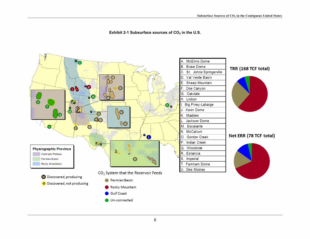
2 Discovered Sources of Geologic CO2 Most CO2 deposits discovered to date have been the by-product of exploration efforts for hydrocarbons. A survey of public-domain literature identified 21 fields or structures containing geologic CO2 resources. An index map showing the status of the fields is shown in Exhibit 2-1. In the following section, each of the fields or structures is described by region in general order of size. The regions examined are the Rocky Mountains, Colorado Plateau, Permian Basin and other discoveries. A field location map is provided in Appendix 1 for each field; the maps are presented at the same scale to aid in the appreciation and understanding their relative size.
7
Subsurface Sources of CO2 in the Contiguous United States
Exhibit 2-1 Subsurface sources of CO2 in the U.S.
8
Subsurface Sources of CO2 in the Contiguous United States
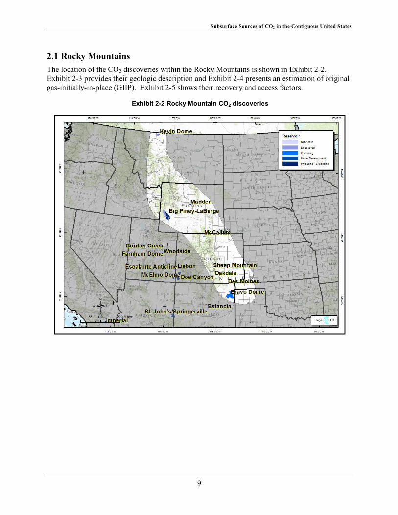
2.1 Rocky Mountains The location of the CO2 discoveries within the Rocky Mountains is shown in Exhibit 2-2. Exhibit 2-3 provides their geologic description and Exhibit 2-4 presents an estimation of original gas-initially-in-place (GIIP). Exhibit 2-5 shows their recovery and access factors.
Exhibit 2-2 Rocky Mountain CO2 discoveries
9
Subsurface Sources of CO2 in the Contiguous United States
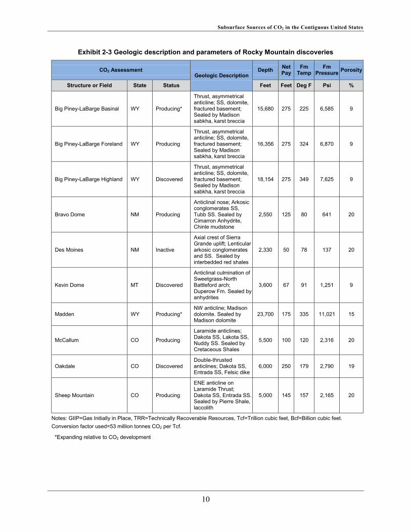
Exhibit 2-3 Geologic description and parameters of Rocky Mountain discoveries
CO2 Assessment Geologic Description
Depth Net Pay
Fm Temp
Fm Pressure Porosity
Structure or Field State Status Feet Feet Deg F Psi %
Big Piney-LaBarge Basinal WY Producing*
Thrust, asymmetrical anticline; SS, dolomite, fractured basement; Sealed by Madison sabkha, karst breccia
15,680 275 225 6,585 9
Big Piney-LaBarge Foreland WY Producing
Thrust, asymmetrical anticline; SS, dolomite, fractured basement; Sealed by Madison sabkha, karst breccia
16,356 275 324 6,870 9
Big Piney-LaBarge Highland WY Discovered
Thrust, asymmetrical anticline; SS, dolomite, fractured basement; Sealed by Madison sabkha, karst breccia
18,154 275 349 7,625 9
Bravo Dome NM Producing
Anticlinal nose; Arkosic conglomerates SS, Tubb SS. Sealed by Cimarron Anhydrite, Chinle mudstone
2,550 125 80 641 20
Des Moines NM Inactive
Axial crest of Sierra Grande uplift; Lenticular arkosic conglomerates and SS. Sealed by interbedded red shales
2,330 50 78 137 20
Kevin Dome MT Discovered
Anticlinal culmination of Sweetgrass-North Battleford arch; Duperow Fm. Sealed by anhydrites
3,600 67 91 1,251 9
Madden WY Producing* NW anticline; Madison dolomite. Sealed by Madison dolomite
23,700 175 335 11,021 15
McCallum CO Producing
Laramide anticlines; Dakota SS, Lakota SS, Nuddy SS. Sealed by Cretaceous Shales
5,500 100 120 2,316 20
Oakdale CO Discovered Double-thrusted anticlines; Dakota SS, Entrada SS, Felsic dike
6,000 250 179 2,790 19
Sheep Mountain CO Producing
ENE anticline on Laramide Thrust; Dakota SS, Entrada SS. Sealed by Pierre Shale, laccolith
5,000 145 157 2,165 20
Notes: GIIP=Gas Initially in Place, TRR=Technically Recoverable Resources, Tcf=Trillion cubic feet, Bcf=Billion cubic feet. Conversion factor used=53 million tonnes CO2 per Tcf.
*Expanding relative to CO2 development
10
Subsurface Sources of CO2 in the Contiguous United States
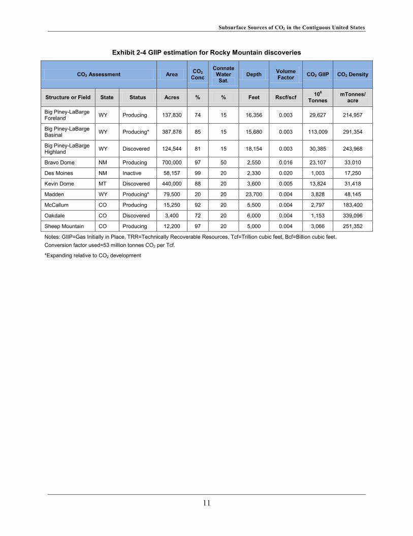
Exhibit 2-4 GIIP estimation for Rocky Mountain discoveries
CO2 Assessment Area CO2 Conc
Connate Water Sat.
Depth Volume Factor CO2 GIIP CO2 Density
Structure or Field State Status Acres % % Feet Rscf/scf 106 Tonnes
mTonnes/ acre
Big Piney-LaBarge Foreland WY Producing 137,830 74 15 16,356 0.003 29,627 214,957
Big Piney-LaBarge Basinal WY Producing* 387,876 85 15 15,680 0.003 113,009 291,354
Big Piney-LaBarge Highland WY Discovered 124,544 81 15 18,154 0.003 30,385 243,968
Bravo Dome NM Producing 700,000 97 50 2,550 0.016 23,107 33,010
Des Moines NM Inactive 58,157 99 20 2,330 0.020 1,003 17,250
Kevin Dome MT Discovered 440,000 88 20 3,600 0.005 13,824 31,418
Madden WY Producing* 79,500 20 20 23,700 0.004 3,828 48,145
McCallum CO Producing 15,250 92 20 5,500 0.004 2,797 183,400
Oakdale CO Discovered 3,400 72 20 6,000 0.004 1,153 339,096
Sheep Mountain CO Producing 12,200 97 20 5,000 0.004 3,066 251,352
Notes: GIIP=Gas Initially in Place, TRR=Technically Recoverable Resources, Tcf=Trillion cubic feet, Bcf=Billion cubic feet. Conversion factor used=53 million tonnes CO2 per Tcf.
*Expanding relative to CO2 development
11
Subsurface Sources of CO2 in the Contiguous United States
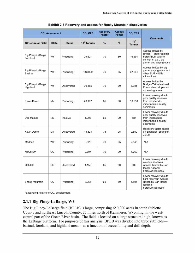
Exhibit 2-5 Recovery and access for Rocky Mountain discoveries
CO2 Assessment CO2 GIIP Recovery Factor
Access Factor CO2 TRR
Comments
Structure or Field State Status 106 Tonnes % % 106 Tonnes
Big Piney-LaBarge Foreland WY Producing 29,627 70 80 16,591
Access limited by Bridger-Teton National Forest\BLM wildlife concerns, e.g., big game, and sage grouse
Big Piney-LaBarge Basinal WY Producing* 113,009 70 85 67,241
Access limited by big game, sage grouse and other BLM wildlife stipulations
Big Piney-LaBarge Highland WY Discovered 30,385 70 30 6,381
Access limited by Bridger-Teton National Forest steep slopes and no leasing areas
Bravo Dome NM Producing 23,107 65 90 13,518
Lower recovery due to poor quality reservoir from interbedded impermeable muddy sediments
Des Moines NM Inactive 1,003 65 90 587
Lower recovery due to poor quality reservoir from interbedded impermeable muddy sediments
Kevin Dome MT Discovered 13,824 75 95 9,850 Recovery factor based on Spangler (Spangler, 2012)
Madden WY Producing* 3,828 70 95 2,545 N/A
McCallum CO Producing 2,797 70 90 1,762 N/A
Oakdale CO Discovered 1,153 65 80 600
Lower recovery due to volcanic reservoir. Access limited by San Isabel National Forest/Wilderness
Sheep Mountain CO Producing 3,066 65 80 1,595
Lower recovery due to tight reservoir. Access limited by San Isabel National Forest/Wilderness
*Expanding relative to CO2 development
2.1.1 Big Piney-LaBarge, WY The Big Piney-LaBarge field (BPLB) is large, comprising 650,000 acres in south Sublette County and northeast Lincoln County, 25 miles north of Kemmerer, Wyoming, in the west-central part of the Green River basin. The field is located on a large structural high, known as the LaBarge platform. For purposes of this analysis, BPLB was divided into three subfields—basinal, foreland, and highland areas—as a function of accessibility and drill depth.
12
Subsurface Sources of CO2 in the Contiguous United States
In BPLB, the reservoir is the Mississippian Madison Formation, which comprises a thick carbonate reservoir, ranging from 14,000 feet below surface in the southwest and plunging to 19,000 feet in the northeast. The lower Madison Formation is made up of shallow-shelf dolomitized limestone and dolomite. The reservoirs are overlain and sealed by the Upper Madison sabkha deposits. The trap is a large anticline with a relatively steeper dips on its west flank, where it is bounded by an east-dipping thrust fault. (Denbury, July 2013) Porosity ranges from 6 to 12 percent (Stilwell, 1989); permeability is 10 to 50 mD. (Denbury, July 2013) Prior to Tertiary deposition, the LaBarge platform was a large doubly-plunging anticline. Subsidence of the Green River basin to the northeast followed by Tertiary deposition has resulted in generally east-northeast dips. The western flank of the LaBarge platform has been modified by thrust faulting. A number of anticlinal folds with associated high-angle reverse faults and tear faults have been encountered on the platform. On some of these folds, such as the one defining the LaBarge field, the initial movement was prior to Tertiary deposition, and the associated reverse faulting is upthrown to the east.
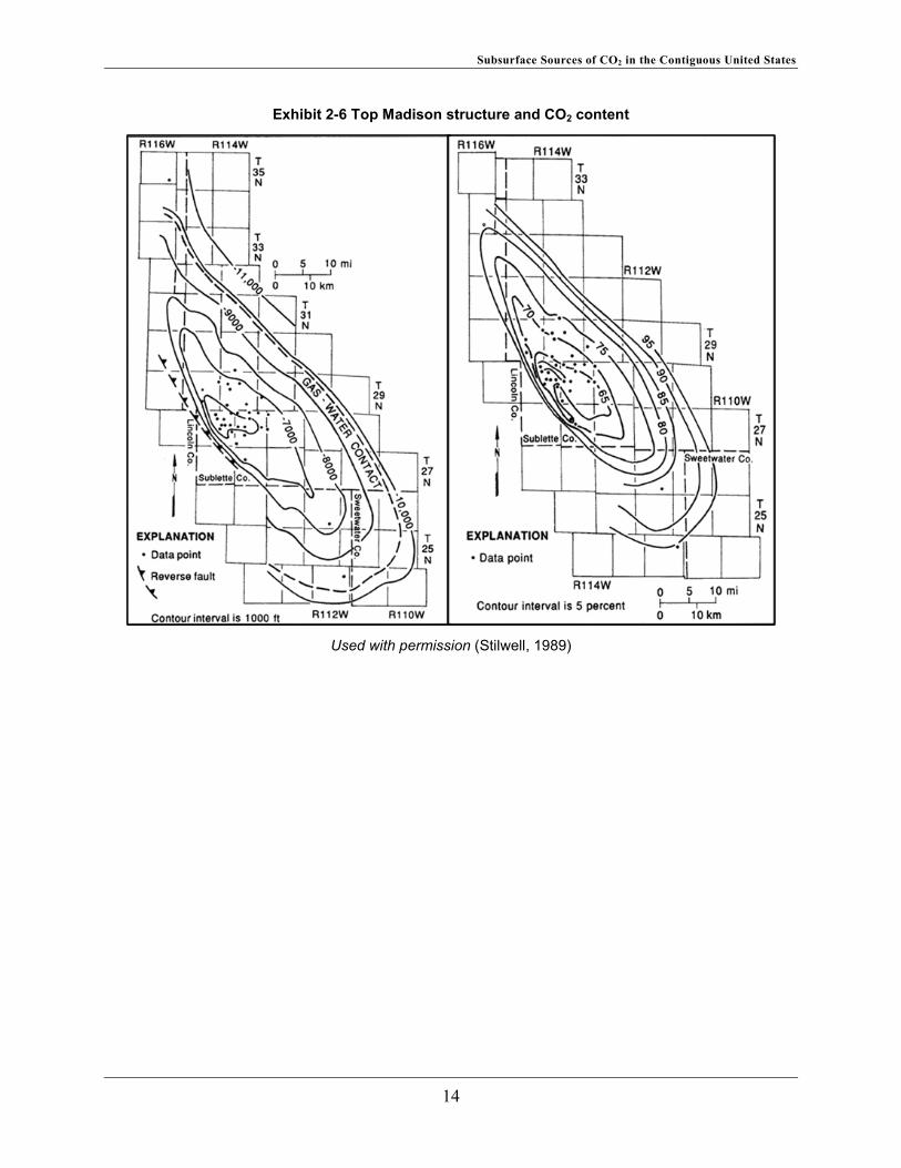
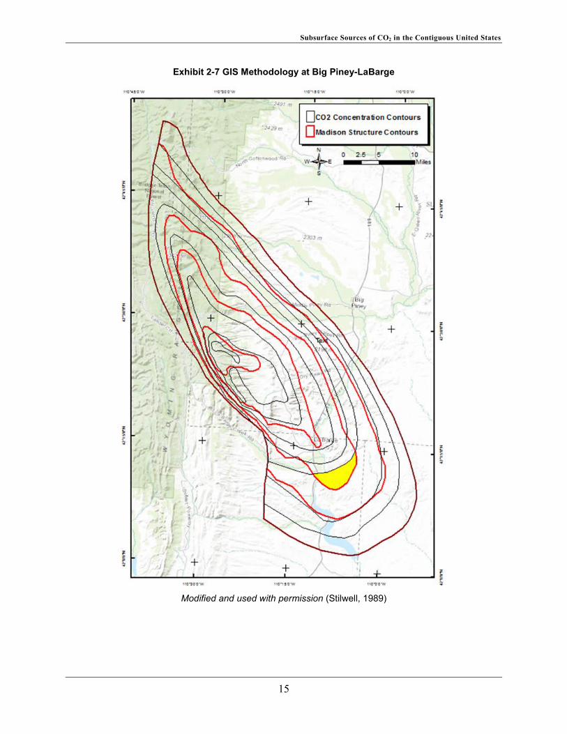
Stilwell presents a top Madison structure map along with a corresponding CO2 concentration map, shown in Exhibit 2-6. (Stilwell, 1989) These maps were integrated in a Geographical Information System (GIS) along with the topographic information. The resultant polygons were attributed and modeled with discrete combinations of drill depth and CO2 concentration. The accessibility of resources for actual drilling was also incorporated into the GIS as discussed in Section 3, which shows an example for BPLB. Exhibit 2-7 shows the GIS-based analysis performed, resulting in the attributes of the highlighted polygon.
Drilling activity in the Big Piney gas field began in 1952, and was successful with the market provided by the Pacific Northwest natural gas pipeline, running from the San Juan basin in southern Colorado to the state of Washington. (Stilwell, 1989) Today, the Big Piney-LaBarge complex, consisting of the Tiptop, Dry Piney, Hogsback, LaBarge, and Big Piney oil and gas fields, produces to the Shute Creek gas plant with a natural gas capacity of 600 million cubic feet per day (MMcfd). ExxonMobil’s average well produces 45 MMcfd, (Khayyal, July 2013) with which modeling presented in this report is consistent. Sales capacity at Shute Creek is 340 MMcfd. The gas processed is typically two-thirds CO2. Approximately 100 MMcfd CO2 is piped to Rangely oil field in Colorado, (NETL, undated) and 75 MMcfd is piped to Lost Soldier and Wertz oil fields in Wyoming, for tertiary oil recovery. In the past, about 225 MMcfd of CO2 were vented to the atmosphere due to a lack of markets, (NETL, undated) a situation that is changing with the increased demand for CO2 in EOR. The field currently produces about 215 MMcfd of CO2, and ExxonMobil is installing increased compression capability (Condon, 2011) to address the EOR markets. CO2 production is also established at the Riley Ridge facility, operated by Denbury Resources. (Denbury, 2012) In addition to CO2, produced gases include helium and H2S. The H2S is re-injected. It is assumed that in modeling this field, costs associated with H2S reinjection are three-quarters that of sulfur extraction.
13
Subsurface Sources of CO2 in the Contiguous United States
Exhibit 2-6 Top Madison structure and CO2 content
Used with permission (Stilwell, 1989)
14
Subsurface Sources of CO2 in the Contiguous United States
Exhibit 2-7 GIS Methodology at Big Piney-LaBarge
Modified and used with permission (Stilwell, 1989)
15
Subsurface Sources of CO2 in the Contiguous United States
2.1.2 Bravo Dome, NM Bravo Dome (originally the Bueyeros field) is a large field, comprising 700,000 acres located in Union, Harding, and Quay Counties, 30 miles to the southwest of Clayton, New Mexico. Bravo Dome is a northwest-trending anticlinal nose situated on the spur of the Sierra Grande arch. The region is bounded by the Tucumari basin to the south and the Dalhart basin to the north.
Bravo Dome field is a combination structural stratigraphic trap caused by the thinning and loss of permeability in the Permian Tubb Sandstone to north and west across a southeast plunging arch on the east edge of the Sierra Grande uplift. The reservoir is scaled below by granite in the west and by impermeable shales and tight sandstones in the east. It is sealed above by impermeable anhydrite of the Cimmaron Anhydrite and shales of the Upper Clearfork Formation (Cassidy, 2005). Bravo Dome produces from the Permian Tubb Formation at relatively shallow depths of around 2,550 feet. (Broadhead, 2009) The Tubb Formation is an arkosic sandstone formed by sand-dominated alluvial, fluvial, and eolian deposition with an average thickness of 125 feet. (Cassidy, 2005) (Zimmerman, 1979) (NETL, undated) Tubb deposition apparently did not occur to the northwest of the structure, resulting in a depositional pinch-out on the Sierra Grande Uplift. Tubb thickness increases rapidly down-dip, to a maximum of 500 feet in the southeastern portion of the structure. The Tubb pinch-out limits productivity in the northwestern portion of the structure. An apparent gas water contact limits productivity down-dip in the southeastern and southwestern portions of the structure.
CO2 is trapped by a combination of stratigraphic pinch-out and fold closures. The reservoir is sealed by the impervious Cimarron anhydrite, which is a mixture of shallow marine evaporates and arkosic muds. Average porosity and permeability are 20 percent and 42 millidarcy (mD) respectively. (NETL, undated)
Bravo Dome was accidentally discovered in 1916, during petroleum exploration; development commenced in 1931. It was expanded throughout the 1930s to 19 wells, which produced modestly until the end of the 1970s. An additional 270 wells were drilled in the 1980s, in order to satisfy the demand for CO2 for EOR in west Texas. (Broadhead, 2009) Production is approximately 120 billion cubic feet (Bcf) per year from 250 wells. (Broadhead, 2009)
2.1.3 Des Moines, NM The Des Moines field is located in northwestern Union County, 35 miles east of Raton, New Mexico, and 35 miles northwest of Bravo Dome. The field is located near the axial crest of the Sierra Grande uplift. The primary reservoirs are lenticular arkosic conglomerates and conglomeratic sandstones of the Permian Abo Formation. The formation rests unconformably on Precambrian basement in the area. Interbedded red shales act as seals. Depth to production averages 2,300 feet, with 50 to feet of net pay. (Broadhead, 2009)
The field was discovered in 1935. Four additional productive wells were drilled during the 1950s, and a processing plant was built to convert the CO2 into liquid CO2 and dry ice. (Broadhead, 2009) The field produced until 1966, when it was abandoned because of problems related to gas processing. Cumulative production from the Des Moines field is estimated to have produced about 20 Bcf.
16
Subsurface Sources of CO2 in the Contiguous United States
2.1.4 Kevin Dome, MT Kevin Dome is located on the western flank of the Williston basin along the U.S.-Canadian border in southwestern Saskatchewan and northern Montana, 30 miles northwest of Havre, Montana. The majority of the field is located in Canada with its southern extent located in the U.S. In the area of Kevin Dome, the structure of western North America has been influenced by crustal shortening associated with the Antler orogeny in Upper Devonian time. Further crustal shortening and uplift occurred in the region during the Laramide orogeny in early Tertiary Time. In Montana, major structural elements include the north-trending Sweetgrass–North Battleford arch, (Lake, 2006) upon which Kevin Dome is a large anticlinal culmination along its axis. The deposit covers over 280,000 acres with approximately 750 feet of structural relief. The area of Kevin Dome was calculated based on Spangler (Spangler, 2012) and a Montana Geological Society (MGS, 1985) structural map on the Madison Formation, assuming persistent compartmentalization at the Duperow level, and a tightening of the fold with depth. As discussed in Section 3.2.2, wells drilled in the Upper Duperow are dual-completed in the Lower Duperow formation.
At Kevin Dome, the Duperow Formation shows facies variability both laterally and vertically that results in thin, widespread depositional cycles that are suggestive of a stable cratonic and climatic environment. Duperow strata generally exhibit shallowing-upward cycles of carbonate deposition in very shallow settings that often are capped by evaporite deposits. These anhydrite-dominated layers at the top of individual cycles often serve as effective seals to fluid migration. (Lake, 2006)
Geologically occurring CO2 has been documented in several oil and gas wells drilled over the past 50 years, which have penetrated the Upper Devonian Duperow Formation, although reservoir characteristics are not well understood. The Duperow averages 75 feet of net thickness with 9 percent porosity. Gases average 88 percent CO2 with the balance of gas being nitrogen. (Spangler, 2012)
2.1.5 Madden, WY The Madden gas field is in the Wind River basin, in Fremont County, fifteen miles north-northeast of Shoshoni, Wyoming. The double-plunging Madden anticline was a deep basin play beneath the southwest vergent Wind River thrust. Produced natural gases from the Madden field contain 67 percent methane and about 20 percent CO2. Conoco Phillips previously vented 50 MMcfd from its Lost Cabin Gas Processing facility, (ConocoPhillips, undated) which is now being converted to capture CO2 for use in EOR. According to Conoco-Phillips, sulfur derived from production at the field is marketed. (ConocoPhillips, undated)
2.1.6 McCallum, CO McCallum anticline is a modest-sized field located in McCallum County, 50 miles northwest of Estes Park, Colorado, in the North Park basin. The field comprises two large anticlines, North McCallum anticline, and the faulted en-echelon South McCallum anticline that is structurally juxtaposed on the southeast. CO2 is trapped in late Laramide-related anticlines and faulted anticlines in a combination of structural and stratigraphic traps. (Stevens, May 15-17, 2001)
The field produces from the Lower Cretaceous Dakota and Lakota formations. The reservoirs average 5,500 feet in depth and about 100 feet net thickness. (Gilfillan, 2008) The Dakota
17
Subsurface Sources of CO2 in the Contiguous United States
Sandstone consists of intertongued beds of fluvial shoreline sandstone, carbonaceous siltstone, claystone, and conglomeratic sandstone. Individual reservoir thicknesses average 25-40 feet, with an average porosity of 18 to 20 percent. (Wandrey, undated) The Lakota Sandstone consists of medium-to-coarse-grained sandstone and conglomerate. Reservoir thicknesses average about 100 feet. (Wandrey, undated)
The field was first discovered in 1925, and has produced approximately 870 Bcf of CO2 since 1927. As of 2001, four wells were in operation with the field producing around 38 Bcf per year of CO2 for industrial use. (Stevens, May 15-17, 2001)
2.1.7 Oakdale, CO Oakdale is a small (3,400 acres) field located in the northern Raton basin, in Huerfano County, 20 miles west-southwest of Walsenburg, Colorado, and five miles southeast of the larger Sheep Mountain field. The field is a subthrust play and consists of a double-thrusted anticline located in the footwall of the Sangre de Cristo (main) thrust and in the hanging-wall of the Oakdale thrust. The Raton basin sedimentary succession was folded and thrust faulted during the Laramide orogeny (Late Cretaceous through Eocene time) when the Sangre de Cristo Mountains were formed. The thrusting and folding that formed the north-northwest to south-southeast trending, double-plunging Oakdale anticline is the product of at least two episodes of thrust faulting. (Worrall, 2003)
Pay zones include the Dakota and Entrada sandstones and one unconventional zone, which is a three-hundred-feet thick, shallow-dipping, felsite dike that has both primary and secondary fracture porosity and permeability. The Dakota Sandstone is typically about 200 feet thick within and around the north Raton basin. It consists of two beds of white-to-buff, well-sorted, cross-stratified, fine-to-medium grained, quartzitic sandstone, and a very thin interbed of black carbonaceous shale. (USGS, 1959) The much thinner and less continuous Entrada Sandstone is slightly less than 100 feet thick. The Entrada sandstone lies disconformably on the uppermost red beds of the Sangre de Cristo Formation. The formation consists of light-gray-to-buff, thick-to-massive, well-rounded, fine-to-medium grained quartzitic sandstone. The formation tends to increase in thickness toward the north and northeast of Oakdale (Johnson, 1959). Both the Dakota and Entrada Sandstone reservoirs have twice as much porosity as typically seen elsewhere in the Raton basin.
Each of the three reservoirs at Oakdale contains gases of radically different composition, varying from 24 percent to 97 percent CO2, and 3 percent to 75 percent oil or methane. The small (370 acres) microgranite Maestas stock and associated dikes are the likely “source rocks” for the adjoining, primitive, 3He-bearing CO2 gas found at Oakdale and Sheep Mountain. Worrall estimated total reserves for the Dakota and Entrada sandstones at 450 Bcf in place with a gas column of 1,000 feet. (Worrall, 2003) All three reservoirs (the Dakota and Entrada formations and the felsites dike) were evaluated in this assessment based on estimated average properties for the three units.
2.1.8 Sheep Mountain, CO The Sheep Mountain gas field is located at the northern end of the Raton basin, in Huerfano County, 20 miles west of Walsenberg, Colorado, and five miles northwest of the Oakdale field. The Sheep Mountain and Oakdale anticlines are subthrust anticlines beneath the Sangre de Cristo
18
Subsurface Sources of CO2 in the Contiguous United States
thrust. These upright, open, double-plunging foreland folds are aligned along a common northwest-trending axial trace and are Laramide-aged (60-45 millions of years ago (Ma)) imbricate thrusted folds, which share common styles and modes of deformation.
The Raton basin sedimentary succession was folded and thrust-faulted during the Laramide orogeny when the Sangre de Cristo Mountains were formed. Folding and overthrusting created the Malachite syncline and the little Sheep Mountain anticline. This northwest-trending anticlinal fold is bounded on the northeast side by a minor thrust fault and forms the structural trap of the field.
Methane and CO2 gases and oil are reservoired within the 70-feet-thick Entrada and 200-feet-thick Dakota sandstones as well as an overlying, shallow west southwest-dipping, 300 feet thick, Oligocene felsite dike emplaced along and within the low-angle west southwest-dipping La Veta thrust. Combined, the three formations comprise 145 feet of net pay. The dike is highly fractured and shows good fracture permeability and porosity as well as primary intra-matrix porosity. This unusual reservoir is viewed as a significant component of the CO2 resource at the nearby Oakdale field. (USGS, 2007) The reservoir produces at an average depth of 5,000 feet (Broadhead, 2009). Gases are 97 percent CO2 with 2 percent N2.
Production began in 1983, and has continued at an average rate of 70 Bcf/year, with cumulative production to 1999 estimated at 1.2 Tcf. (NETL, undated) The gas is refined and pumped via pipeline to west Texas, where it is used for EOR.
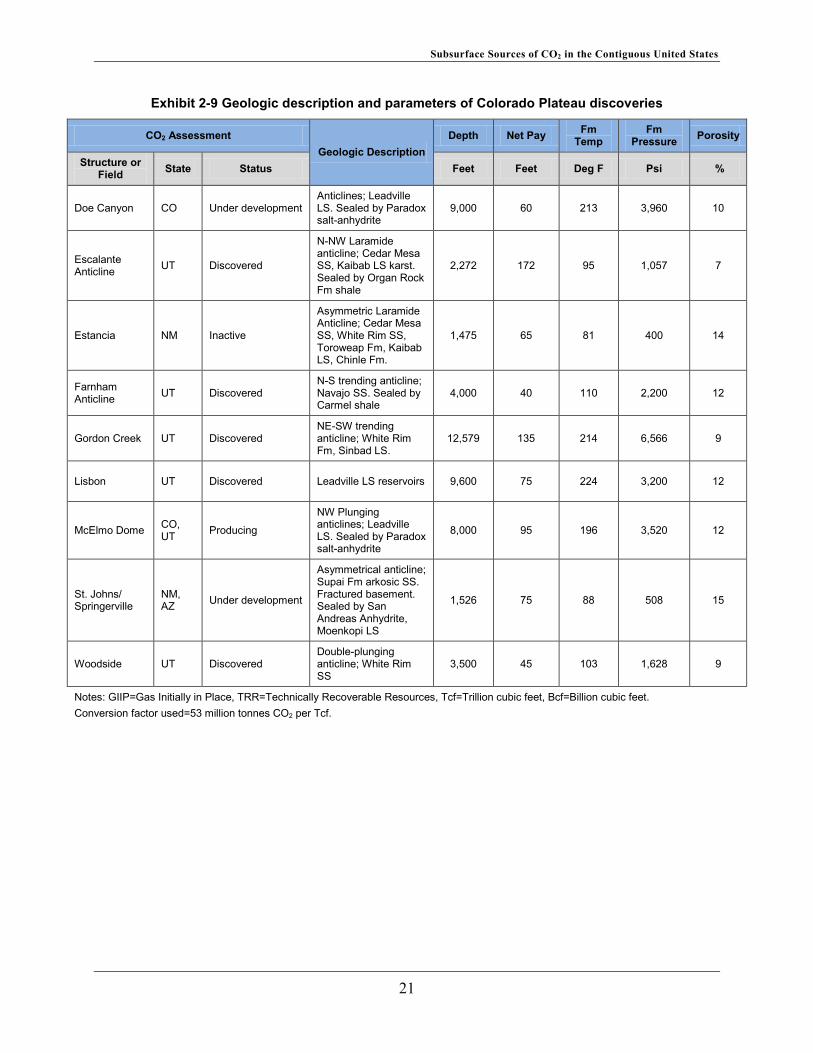
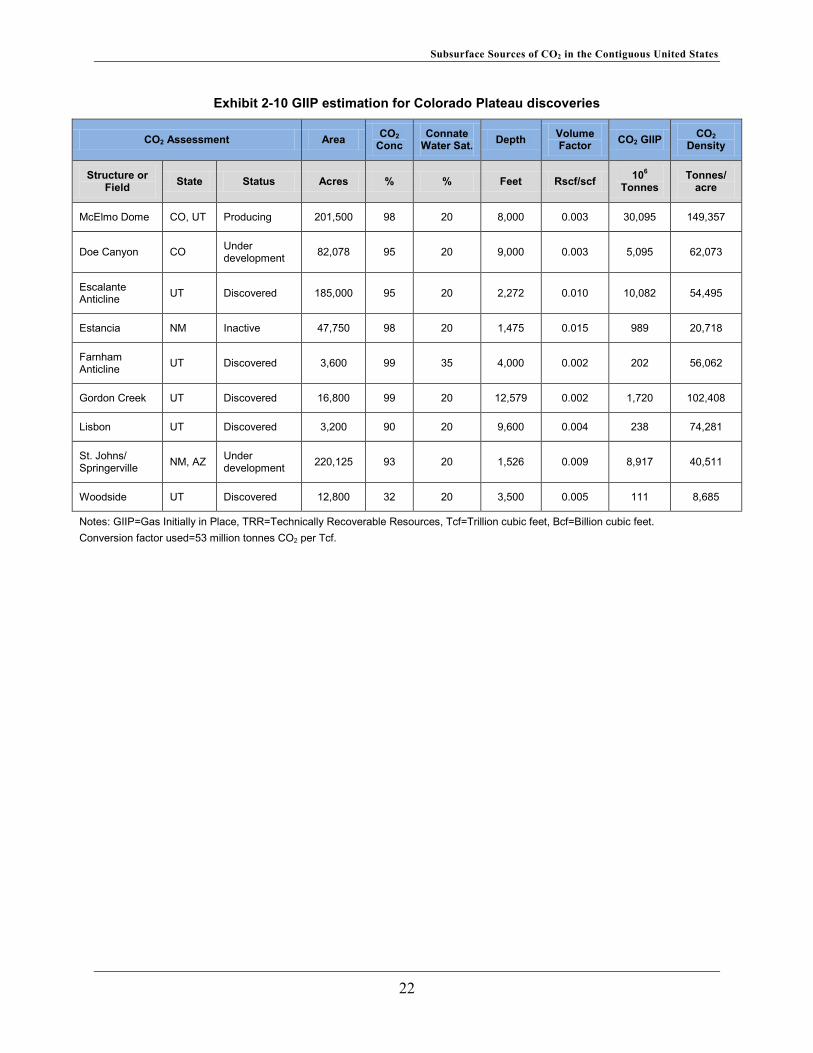
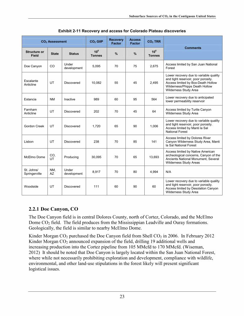
2.2 Colorado Plateau The location of the CO2 discoveries within the Colorado Plateau is shown in Exhibit 2-8. Exhibit 2-9 provides their geologic description and Exhibit 2-10 presents an estimation of original GIIP. Exhibit 2-11 shows their recovery and access factors.
19

Subsurface Sources of CO2 in the Contiguous United States
Exhibit 2-8 Colorado Plateau CO2 discoveries
20
Subsurface Sources of CO2 in the Contiguous United States
Exhibit 2-9 Geologic description and parameters of Colorado Plateau discoveries
CO2 Assessment Geologic Description
Depth Net Pay Fm Temp
Fm Pressure Porosity
Structure or Field State Status Feet Feet Deg F Psi %
Doe Canyon CO Under development Anticlines; Leadville LS. Sealed by Paradox salt-anhydrite
9,000 60 213 3,960 10
Escalante Anticline UT Discovered
N-NW Laramide anticline; Cedar Mesa SS, Kaibab LS karst. Sealed by Organ Rock Fm shale
2,272 172 95 1,057 7
Estancia NM Inactive
Asymmetric Laramide Anticline; Cedar Mesa SS, White Rim SS, Toroweap Fm, Kaibab LS, Chinle Fm.
1,475 65 81 400 14
Farnham Anticline UT Discovered
N-S trending anticline; Navajo SS. Sealed by Carmel shale
4,000 40 110 2,200 12
Gordon Creek UT Discovered NE-SW trending anticline; White Rim Fm, Sinbad LS.
12,579 135 214 6,566 9
Lisbon UT Discovered Leadville LS reservoirs 9,600 75 224 3,200 12
McElmo Dome CO, UT Producing
NW Plunging anticlines; Leadville LS. Sealed by Paradox salt-anhydrite
8,000 95 196 3,520 12
St. Johns/ Springerville
NM, AZ Under development
Asymmetrical anticline; Supai Fm arkosic SS. Fractured basement. Sealed by San Andreas Anhydrite, Moenkopi LS
1,526 75 88 508 15
Woodside UT Discovered Double-plunging anticline; White Rim SS
3,500 45 103 1,628 9
Notes: GIIP=Gas Initially in Place, TRR=Technically Recoverable Resources, Tcf=Trillion cubic feet, Bcf=Billion cubic feet. Conversion factor used=53 million tonnes CO2 per Tcf.
21
Subsurface Sources of CO2 in the Contiguous United States
Exhibit 2-10 GIIP estimation for Colorado Plateau discoveries
CO2 Assessment Area CO2 Conc
Connate Water Sat. Depth Volume
Factor CO2 GIIP CO2 Density
Structure or Field State Status Acres % % Feet Rscf/scf 106
Tonnes Tonnes/
acre
McElmo Dome CO, UT Producing 201,500 98 20 8,000 0.003 30,095 149,357
Doe Canyon CO Under development 82,078 95 20 9,000 0.003 5,095 62,073
Escalante Anticline UT Discovered 185,000 95 20 2,272 0.010 10,082 54,495
Estancia NM Inactive 47,750 98 20 1,475 0.015 989 20,718
Farnham Anticline UT Discovered 3,600 99 35 4,000 0.002 202 56,062
Gordon Creek UT Discovered 16,800 99 20 12,579 0.002 1,720 102,408
Lisbon UT Discovered 3,200 90 20 9,600 0.004 238 74,281
St. Johns/ Springerville NM, AZ Under
development 220,125 93 20 1,526 0.009 8,917 40,511
Woodside UT Discovered 12,800 32 20 3,500 0.005 111 8,685
Notes: GIIP=Gas Initially in Place, TRR=Technically Recoverable Resources, Tcf=Trillion cubic feet, Bcf=Billion cubic feet. Conversion factor used=53 million tonnes CO2 per Tcf.
22
Subsurface Sources of CO2 in the Contiguous United States
Exhibit 2-11 Recovery and access for Colorado Plateau discoveries
CO2 Assessment CO2 GIIP Recovery Factor
Access Factor CO2 TRR
Comments Structure or
Field State Status 106 Tonnes % % 106
Tonnes
Doe Canyon CO Under development 5,095 70 75 2,675 Access limited by San Juan National
Forest
Escalante Anticline UT Discovered 10,082 55 45 2,495
Lower recovery due to variable quality and tight reservoir, poor porosity. Access limited by Box-Death Hollow Wilderness/Phipps Death Hollow Wilderness Study Area
Estancia NM Inactive 989 60 95 564 Lower recovery due to anticipated lower permeability reservoir
Farnham Anticline UT Discovered 202 70 45 64 Access limited by Turtle Canyon
Wilderness Study Area
Gordon Creek UT Discovered 1,720 65 90 1,006
Lower recovery due to variable quality and tight reservoir, poor porosity. Access limited by Manti la Sal National Forest
Lisbon UT Discovered 238 70 85 141 Access limited by Dolores River Canyon Wilderness Study Area, Manti la Sal National Forest
McElmo Dome CO, UT Producing 30,095 70 65 13,693
Access limited by Native American archeological concerns, Canyon of the Ancients National Monument, Several Wilderness Study Areas
St. Johns/ Springerville
NM, AZ
Under development 8,917 70 80 4,994 N/A
Woodside UT Discovered 111 60 90 60
Lower recovery due to variable quality and tight reservoir, poor porosity. Access limited by Desolation Canyon Wilderness Study Area
2.2.1 Doe Canyon, CO The Doe Canyon field is in central Dolores County, north of Cortez, Colorado, and the McElmo Dome CO2 field. The field produces from the Mississippian Leadville and Ouray formations. Geologically, the field is similar to nearby McElmo Dome.
Kinder Morgan CO2 purchased the Doe Canyon field from Shell CO2 in 2006. In February 2012 Kinder Morgan CO2 announced expansion of the field, drilling 19 additional wells and increasing production into the Cortez pipeline from 105 MMcfd to 170 MMcfd. (Wiseman, 2012) It should be noted that Doe Canyon is largely located within the San Juan National Forest, where while not necessarily prohibiting exploration and development, compliance with wildlife, environmental, and other land-use stipulations in the forest likely will present significant logistical issues.
23
Subsurface Sources of CO2 in the Contiguous United States
2.2.2 Escalante Anticline, UT The Escalante anticline is located in central Garfield County in southern Utah, 20 miles southwest of Capital Reef National Park. The structure is located in the northern Kaiparowits basin and covers 37,000 acres. The anticline is asymmetric with steepest dips vergent toward the west. It is one of many secondary folds of this Laramide-age structural basin. (NETL, undated)
The Permian and Triassic CO2 reservoirs at Escalante field comprise numerous rock types deposited in a variety of environments. The Permian Cedar Mesa and White Rim sandstones represent near-shore-beach-to-dune deposits and are composed of porous, cross-bedded, fine-to-medium grained sandstone. The Cedar Mesa Sandstone averages 3,150 feet deep with a net thickness of 250 feet. In between the Cedar Mesa and White Rim is the shallow-marine Toroweap Formation. The Toroweap consists of very fine-grained dolomite interbedded with thin, fine-grained sandstone and shale. The Toroweap and White Rim formations average 2,580 feet in depth and 195 feet combined net thickness. The Permian Kaibab limestone was also deposited in a widespread shallow sea. The Kaibab consists of very-fine to fine-grained limestone and dolomite with thin interbedded sandstone and shale. The Kaibab averages 2,300 feet deep and 125 net thickness. The Triassic Timpoweap Member of the Moenkopi Formation is a fine-grained, dense carbonate deposited in a near-shore marine environment. The Timpoweap averages 2,200 feet deep and about 82 feet net thickness. The Shinarump Member of the Triassic Chinle Formation was deposited by northwest-flowing steams in a river flood plain. The Shinarump Member consists of porous, medium-to-coarse grained sandstone. The Shinarump Member averages 1,300 feet deep with 225 feet net thickness.
Gas composition averages about 95 percent CO2 with 2-to-5 percent N2. Porosity ranges from 12-to-16 percent within the sandstone reservoirs to 6-to-8 percent in the carbonates. The potential source of the CO2 in the Escalante anticline is likely magmatic and associated with the High Plateau volcanic province.
The Escalante field was discovered in 1960, by Phillips Petroleum. There has been no production of CO2 from Escalante field.
2.2.3 Estancia Basin, NM The Estancia CO2 fields are located in Torrance County, 25 miles southeast of Edgewood, New Mexico. The two fields are known informally as the northern and the southern Estancia fields and are drilled near the crest of the Wilcox anticline. The structure has been mapped at the surface as a doubly-plunging anticline with 60 to 80 feet of structural closure. The trap appears to be structural, but the down-dip boundaries of the field have never been defined by drilling. It is not known if there is a stratigraphic component to trapping. (NETL, undated) Based on this, the fields were analyzed in this assessment as a single unit.
The northern field was discovered in 1931. Seven productive wells were drilled between 1934 and 1937. (NETL, undated) The reservoirs for the northern Estancia field are associated with sandstones of the Sandia Formation. The produced gas was converted into dry ice at a nearby processing plant.
The southern Estancia field was discovered in 1928. CO2 was encountered between depths of 1,645 feet and 1,760 feet. Although data are vague, it appears that the gas was reservoired by a sandstone bed within the Sandia Formation. In all, three wells produced CO2 from the southern
24

Subsurface Sources of CO2 in the Contiguous United States
Estancia field. The trapping mechanism at the southern Estancia field has not been defined. (NETL, undated)
CO2 was first produced from the Estancia fields in 1934. In that year, a plant was built to convert the CO2 gas into dry ice. The plant produced dry ice until 1942. Cumulative production from the Estancia fields is estimated to be 14 Bcf. (Broadhead, 2009)
2.2.4 Farnham Anticline, UT The small (3,600 acres) Farnham anticline is located in Carbon and Emery Counties, three miles southeast of Price, Utah, in the Uintah basin. It lies 20 miles east of the Gordon Creek field and 20 miles northwest of the Woodside CO2 field. The anticline is asymmetric, west-vergent with a tight, steep forelimb and broad gently-east-dipping backlimb. Reservoirs include the Upper and Lower Jurassic Navajo Sandstone and the Sinbad Limestone Member of the Moenkopi Formation. The average porosity is 12 percent intergranular, in a moderately homogenous eolian sandstone. The trap is both structural and stratigraphic, sealed by interbedded limestone and shale of the Jurassic Carmel Formation. The reservoir averages an estimated 40 feet of net pay, and gas composition is 98.9 percent CO2 with minor N2. (NETL, undated) (Chidsey, 2007)
Production first began in 1931. The field produced 4.8 Bcf, which was pipelined to a nearby dry-ice plant. In 1972, the field was shut in when the dry-ice plant was closed.
2.2.5 Gordon Creek, UT The Gordon Creek field is located in Carbon and Emery counties in the Uintah basin, 10 miles west of Price, Utah, and 20 miles west of the Farnham Dome CO2 field. Gordon Creek was discovered in 1947 has produced 8,500 Mcfd from both the Permian White Rim Sandstone and Sinbad Limestone Member of the Triassic Moenkopi Formation. The trap is a northeast-southwest-trending anticline. The high flow rates from these units suggest the presence of an extensive fracture system.
The White Rim Formation is an eolian dune deposit with an average drill depth of 12,800 feet and 9 percent porosity. (NETL, undated) The Sinbad is a fine-grained, dense carbonate deposited in a near-shore marine environment. It averages 11,000 feet deep and 6 percent porosity. (NETL, undated) CO2 concentrations in both formations are above 98 percent. There has been no production of CO2 from the Gordon Creek field.
2.2.6 Lisbon, UT The Lisbon CO2 fields comprise three small (3,200 total acres) units in San Juan County, Utah and San Miguel County Colorado, 20 miles northeast of Monticello, Colorado. They lie 35 miles northwest of the Doe Canyon field. CO2 is found in the Mississippian Leadville Limestone at an average depth of 9,600 feet. (UGS, 2008)
2.2.7 McElmo Dome, CO, UT McElmo Dome comprises a large anticline with satellite structures, comprising 201,500 acres. It is situated at the southeastern end of the Paradox basin in the Four Corners area, five miles west of Cortez, Colorado, in the center of the Colorado Plateau. The surrounding surface geology is
25
Subsurface Sources of CO2 in the Contiguous United States
dominated by flat-lying sedimentary stratigraphy. It is surrounded by smaller satellite fields to the northwest and west, and the Doe Canyon field to the northeast.
Supercritical CO2 is stored within two productive zones, the Mississippian Leadville and the Devonian Ouray formations, found at depths of 6,500-9,000 feet subsurface. Both formations are composed of limestones and dolomites, with the Leadville providing greater productivity.
Produced gas from both formations comprises 96 to 99 percent CO2 with 1 to 4 percent N2. (NETL, undated) The reservoir structure is complex, consisting of interbedded porous permeable dolomite and tight limestones and less than 100 feet in net thickness (NETL, undated) and averages 8000 feet in depth. (Kinder Morgan CO2, 2013) The trap is a combination of structural closure, permeability barriers within the Leadville, and a 1,200 ft thick salt-cap rock of the Paradox Formation. Porosity averages 12 percent. (NETL, undated)
McElmo Dome was discovered in 1948, and is currently operated by Kinder Morgan CO2. Average annual production since 1995 has ranged from 220–310 Bcf. (NETL, undated) Total cumulative production to date is 7.2 Tcf. (DiPietro, 2012) Commercial production commenced in 1984 with completion of a 500-mile Cortez CO2 pipeline, which supplies CO2 for EOR projects in the Permian basin. A total of 59 CO2 production wells have been drilled at McElmo Dome since 1976. Most wells can deliver 20 MMcfd. The two-phase CO2 present is dehydrated, compressed, and delivered to the Cortez pipeline. (Stevens, May 15-17, 2001) Kinder Morgan CO2 is currently expanding production at the field by 1.2 billion cubic feet per day (Bcfd). (Bradley, 2013)
2.2.8 St. Johns/Springerville, NM, AZ St. Johns Dome is a large (220,000 acre) asymmetrical faulted anticline situated on the southern margin of the Colorado Plateau on the Arizona/New Mexico border, 10 miles northeast of Springerville, Arizona. The field lies on the edge of the Holbrook basin, in the transition zone between the Colorado Plateau and Basin and Range tectonic provinces. CO2 in the field is trapped in the Permian Supai Formation. The Supai Formation is predominantly fine-grained alluvial sandstone interbedded with siltstone, anhydrite, and dolomite. The reservoir is cut by a major northwest-southeast trending reverse fault. Cap rocks in the field are impermeable anhydrites, which vertically separate the CO2 into multiple zones. The reservoir is relatively shallow at about 1500 feet. (Moore, et al., Arizona and New Mexico, Second Annual Conference on Carbon Sequestration. 2003) CO2 in the structure is not in a supercritical state. Gas composition averages 93 percent CO2, along with nitrogen, helium, methane, and argon. (National Academies, 2010)
As described in Stevens et al., 2001, average reservoir porosity is 10 percent, and permeability varies widely, averaging 10 mD and resources are an estimated at 15 Tcf. Moore et al. estimated the porosity as 20 percent. (Moore, et al., Arizona and New Mexico, Second Annual Conference on Carbon Sequestration. 2003) The field was discovered in 1994. Ridgeway Petroleum Corporation drilled 15 wells in Arizona and six wells in New Mexico, which were subsequently shut in.
The company Kinder Morgan CO2 purchased the field and is currently developing it with active drilling at this time. About 40 wells are completed, and a pipeline is planned running either northeast or directly east to tie with the current pipeline system delivering EOR CO2 for Texas.
26
Subsurface Sources of CO2 in the Contiguous United States
The route for the pipeline will be determined by the reserves proved up and the productive capacity of the field following the current drilling campaign. (Bradley, 2011)
2.2.9 Woodside, UT The Woodside field is in Emery County, near the town of Woodside, Utah. It lies 25 miles to the southeast of Farnham anticline. The structure is a crescent-shaped, north-northeast to south-southwest trending, double-plunging anticline with 800 foot of closure and 12,800 acres within the closing contour. (Gilluly, 1929) CO2 is found in the White Rim Sandstone at 3,500 feet at 32 percent concentration. (BLM, 2002)
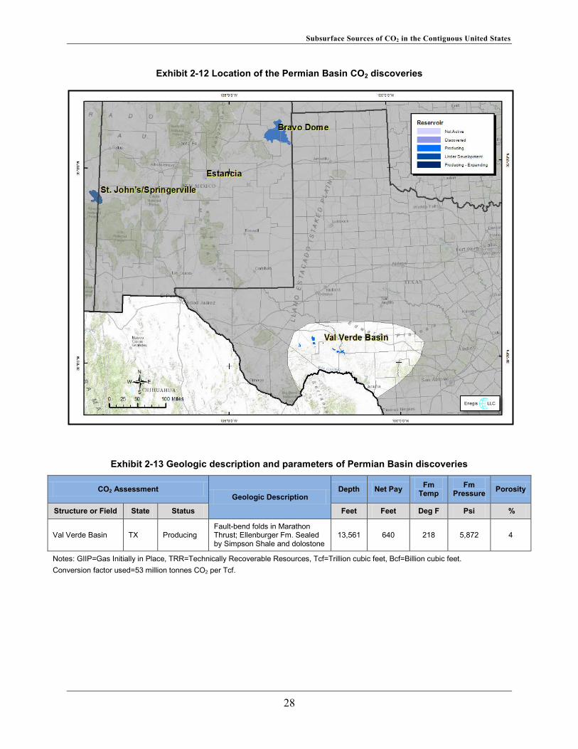
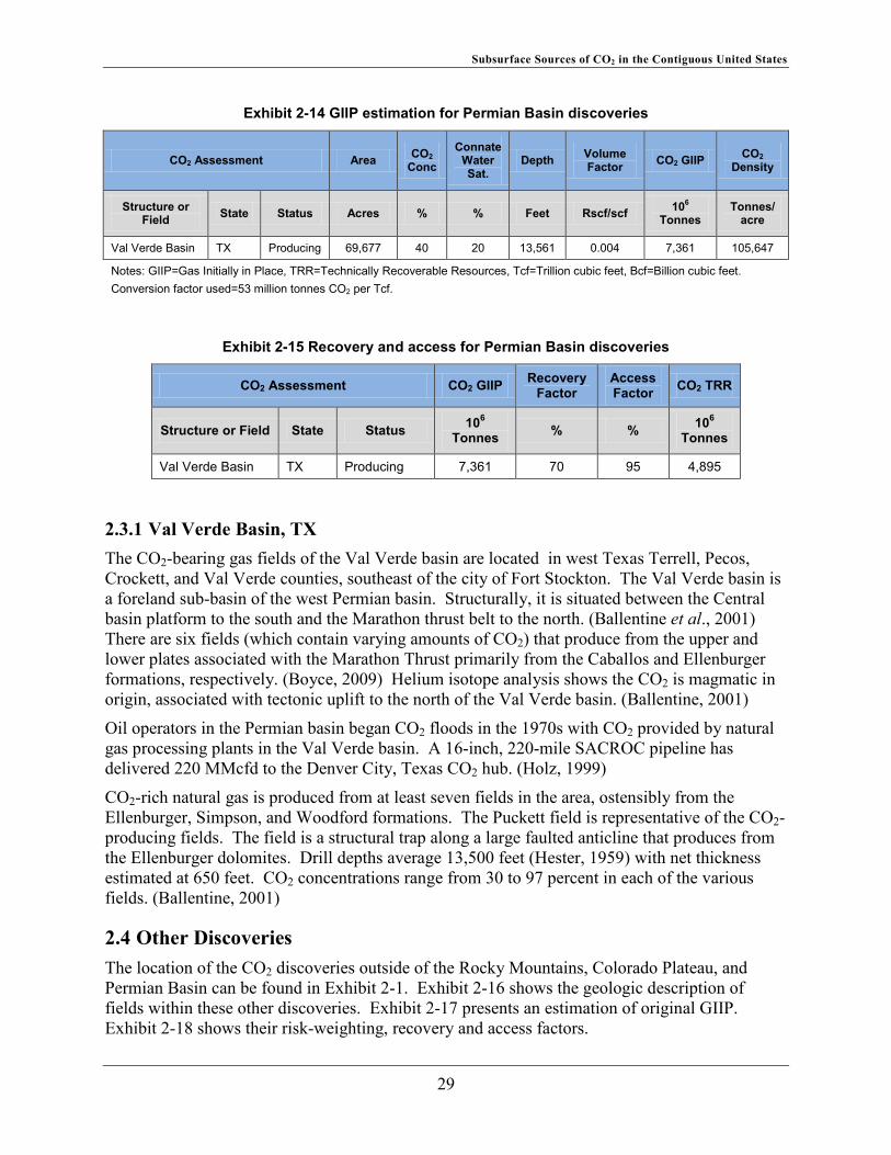
2.3 Permian Basin The location of the Permian basin, of which the Val Verde is a sub-basin, is shown in Exhibit 2-12. Exhibit 2-13 provides a geologic description for the Val Verde basin and Exhibit 2-14 presents its composite estimation of original GIIP. Exhibit 2-15 shows its recovery and access factors.
27
Subsurface Sources of CO2 in the Contiguous United States
Exhibit 2-12 Location of the Permian Basin CO2 discoveries
Exhibit 2-13 Geologic description and parameters of Permian Basin discoveries
CO2 Assessment Geologic Description
Depth Net Pay Fm Temp
Fm Pressure Porosity
Structure or Field State Status Feet Feet Deg F Psi %
Val Verde Basin TX Producing Fault-bend folds in Marathon Thrust; Ellenburger Fm. Sealed by Simpson Shale and dolostone
13,561 640 218 5,872 4
Notes: GIIP=Gas Initially in Place, TRR=Technically Recoverable Resources, Tcf=Trillion cubic feet, Bcf=Billion cubic feet. Conversion factor used=53 million tonnes CO2 per Tcf.
28
Subsurface Sources of CO2 in the Contiguous United States
Exhibit 2-14 GIIP estimation for Permian Basin discoveries
CO2 Assessment Area CO2 Conc
Connate Water Sat.
Depth Volume Factor CO2 GIIP CO2
Density
Structure or Field State Status Acres % % Feet Rscf/scf 106
Tonnes Tonnes/
acre
Val Verde Basin TX Producing 69,677 40 20 13,561 0.004 7,361 105,647
Notes: GIIP=Gas Initially in Place, TRR=Technically Recoverable Resources, Tcf=Trillion cubic feet, Bcf=Billion cubic feet. Conversion factor used=53 million tonnes CO2 per Tcf.
Exhibit 2-15 Recovery and access for Permian Basin discoveries
CO2 Assessment CO2 GIIP Recovery Factor
Access Factor CO2 TRR
Structure or Field State Status 106 Tonnes % % 106
Tonnes
Val Verde Basin TX Producing 7,361 70 95 4,895
2.3.1 Val Verde Basin, TX The CO2-bearing gas fields of the Val Verde basin are located in west Texas Terrell, Pecos, Crockett, and Val Verde counties, southeast of the city of Fort Stockton. The Val Verde basin is a foreland sub-basin of the west Permian basin. Structurally, it is situated between the Central basin platform to the south and the Marathon thrust belt to the north. (Ballentine et al., 2001) There are six fields (which contain varying amounts of CO2) that produce from the upper and lower plates associated with the Marathon Thrust primarily from the Caballos and Ellenburger formations, respectively. (Boyce, 2009) Helium isotope analysis shows the CO2 is magmatic in origin, associated with tectonic uplift to the north of the Val Verde basin. (Ballentine, 2001)
Oil operators in the Permian basin began CO2 floods in the 1970s with CO2 provided by natural gas processing plants in the Val Verde basin. A 16-inch, 220-mile SACROC pipeline has delivered 220 MMcfd to the Denver City, Texas CO2 hub. (Holz, 1999)
CO2-rich natural gas is produced from at least seven fields in the area, ostensibly from the Ellenburger, Simpson, and Woodford formations. The Puckett field is representative of the CO2-producing fields. The field is a structural trap along a large faulted anticline that produces from the Ellenburger dolomites. Drill depths average 13,500 feet (Hester, 1959) with net thickness estimated at 650 feet. CO2 concentrations range from 30 to 97 percent in each of the various fields. (Ballentine, 2001)
2.4 Other Discoveries The location of the CO2 discoveries outside of the Rocky Mountains, Colorado Plateau, and Permian Basin can be found in Exhibit 2-1. Exhibit 2-16 shows the geologic description of fields within these other discoveries. Exhibit 2-17 presents an estimation of original GIIP. Exhibit 2-18 shows their risk-weighting, recovery and access factors.
29

Subsurface Sources of CO2 in the Contiguous United States
Exhibit 2-16 Geologic description and parameters of other discoveries
Exhibit 2-17 GIIP estimation for other discoveries
CO2 Assessment Geologic
Description
Depth Net Pay Fm Temp
Fm Pressure Porosity
Structure or Field State Status Feet Feet Deg F Psi %
Imperial CA Inactive Cenozoic SS reservoirs 591 230 245 339 12
Indian Creek WV Producing Fractured-anticline; Tuscarora Formation 6,674 10 126 3,000 10
Jackson Dome MS Producing*
Anticlines and salt structures; Smackover LS, Norphlet Fm. Sealed by Jurassic mudstone.
15,500 185 339 7,000 13
Notes: GIIP=Gas Initially in Place, TRR=Technically Recoverable Resources, Tcf=Trillion cubic feet, Bcf=Billion cubic feet. Conversion factor used=53 million tonnes CO2 per Tcf.
*Expanding relative to CO2 development
CO2 Assessment Area CO2 Conc
Connate Water Sat.
Depth Volume Factor CO2 GIIP CO2
Density
Structure or Field State Status Acres % % Feet Rscf/scf 106 Tonnes Tonnes/
acre
Indian Creek WV Producing 18,497 66 43 6,674 0.004 85 4,606
Imperial CA Inactive 1,725 95 20 591 0.010 158 91,371
Jackson Dome MS Producing* 90,000 90 20 15,500 0.003 24,245 269,387
Notes: GIIP=Gas Initially in Place, TRR=Technically Recoverable Resources, Tcf=Trillion cubic feet, Bcf=Billion cubic feet. Conversion factor used=53 million tonnes CO2 per Tcf.
*Expanding relative to CO2 development
30
Subsurface Sources of CO2 in the Contiguous United States
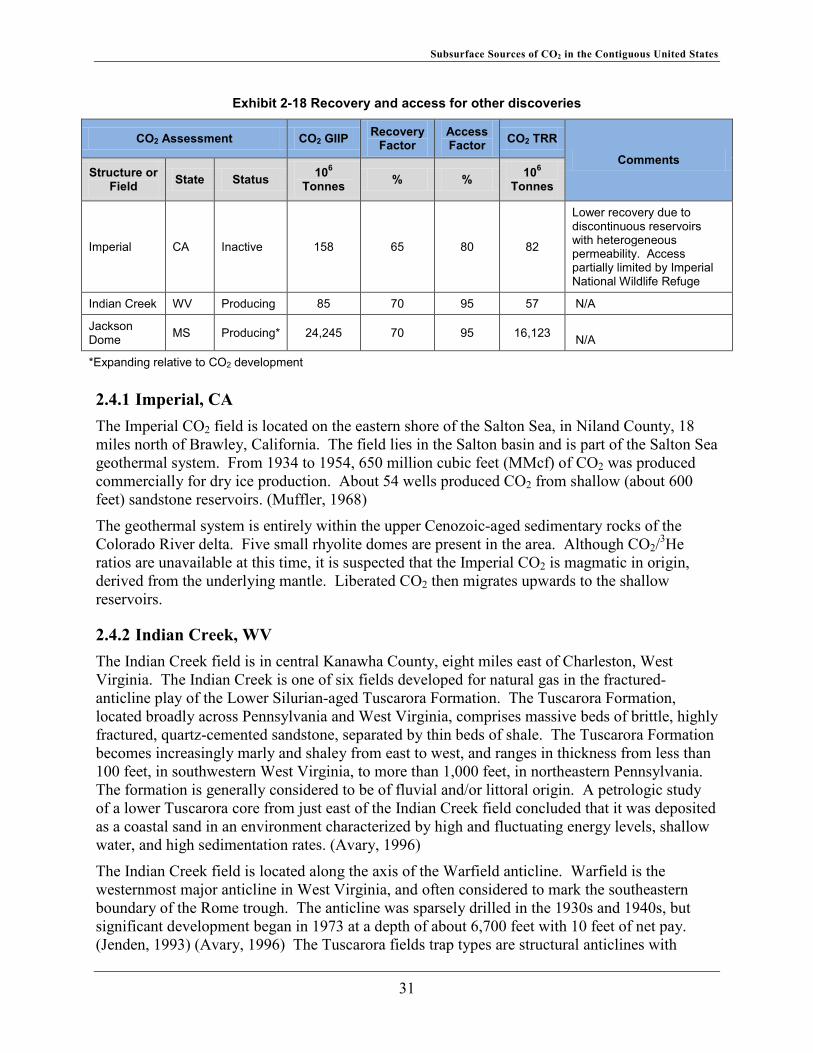
Exhibit 2-18 Recovery and access for other discoveries
CO2 Assessment CO2 GIIP Recovery Factor
Access Factor CO2 TRR
Comments Structure or
Field State Status 106 Tonnes % % 106
Tonnes
Imperial CA Inactive 158 65 80 82
Lower recovery due to discontinuous reservoirs with heterogeneous permeability. Access partially limited by Imperial National Wildlife Refuge
Indian Creek WV Producing 85 70 95 57 N/A
Jackson Dome MS Producing* 24,245 70 95 16,123 N/A
*Expanding relative to CO2 development
2.4.1 Imperial, CA The Imperial CO2 field is located on the eastern shore of the Salton Sea, in Niland County, 18 miles north of Brawley, California. The field lies in the Salton basin and is part of the Salton Sea geothermal system. From 1934 to 1954, 650 million cubic feet (MMcf) of CO2 was produced commercially for dry ice production. About 54 wells produced CO2 from shallow (about 600 feet) sandstone reservoirs. (Muffler, 1968)
The geothermal system is entirely within the upper Cenozoic-aged sedimentary rocks of the Colorado River delta. Five small rhyolite domes are present in the area. Although CO2/3He ratios are unavailable at this time, it is suspected that the Imperial CO2 is magmatic in origin, derived from the underlying mantle. Liberated CO2 then migrates upwards to the shallow reservoirs.
2.4.2 Indian Creek, WV The Indian Creek field is in central Kanawha County, eight miles east of Charleston, West Virginia. The Indian Creek is one of six fields developed for natural gas in the fractured-anticline play of the Lower Silurian-aged Tuscarora Formation. The Tuscarora Formation, located broadly across Pennsylvania and West Virginia, comprises massive beds of brittle, highly fractured, quartz-cemented sandstone, separated by thin beds of shale. The Tuscarora Formation becomes increasingly marly and shaley from east to west, and ranges in thickness from less than 100 feet, in southwestern West Virginia, to more than 1,000 feet, in northeastern Pennsylvania. The formation is generally considered to be of fluvial and/or littoral origin. A petrologic study of a lower Tuscarora core from just east of the Indian Creek field concluded that it was deposited as a coastal sand in an environment characterized by high and fluctuating energy levels, shallow water, and high sedimentation rates. (Avary, 1996)
The Indian Creek field is located along the axis of the Warfield anticline. Warfield is the westernmost major anticline in West Virginia, and often considered to mark the southeastern boundary of the Rome trough. The anticline was sparsely drilled in the 1930s and 1940s, but significant development began in 1973 at a depth of about 6,700 feet with 10 feet of net pay. (Jenden, 1993) (Avary, 1996) The Tuscarora fields trap types are structural anticlines with
31
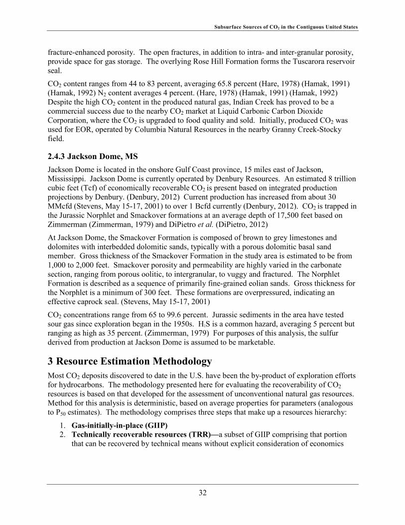
Subsurface Sources of CO2 in the Contiguous United States
fracture-enhanced porosity. The open fractures, in addition to intra- and inter-granular porosity, provide space for gas storage. The overlying Rose Hill Formation forms the Tuscarora reservoir seal.
CO2 content ranges from 44 to 83 percent, averaging 65.8 percent (Hare, 1978) (Hamak, 1991) (Hamak, 1992) N2 content averages 4 percent. (Hare, 1978) (Hamak, 1991) (Hamak, 1992) Despite the high CO2 content in the produced natural gas, Indian Creek has proved to be a commercial success due to the nearby CO2 market at Liquid Carbonic Carbon Dioxide Corporation, where the CO2 is upgraded to food quality and sold. Initially, produced CO2 was used for EOR, operated by Columbia Natural Resources in the nearby Granny Creek-Stocky field.
2.4.3 Jackson Dome, MS Jackson Dome is located in the onshore Gulf Coast province, 15 miles east of Jackson, Mississippi. Jackson Dome is currently operated by Denbury Resources. An estimated 8 trillion cubic feet (Tcf) of economically recoverable CO2 is present based on integrated production projections by Denbury. (Denbury, 2012) Current production has increased from about 30 MMcfd (Stevens, May 15-17, 2001) to over 1 Bcfd currently (Denbury, 2012). CO2 is trapped in the Jurassic Norphlet and Smackover formations at an average depth of 17,500 feet based on Zimmerman (Zimmerman, 1979) and DiPietro et al. (DiPietro, 2012)
At Jackson Dome, the Smackover Formation is composed of brown to grey limestones and dolomites with interbedded dolomitic sands, typically with a porous dolomitic basal sand member. Gross thickness of the Smackover Formation in the study area is estimated to be from 1,000 to 2,000 feet. Smackover porosity and permeability are highly varied in the carbonate section, ranging from porous oolitic, to intergranular, to vuggy and fractured. The Norphlet Formation is described as a sequence of primarily fine-grained eolian sands. Gross thickness for the Norphlet is a minimum of 300 feet. These formations are overpressured, indicating an effective caprock seal. (Stevens, May 15-17, 2001)
CO2 concentrations range from 65 to 99.6 percent. Jurassic sediments in the area have tested sour gas since exploration began in the 1950s. H2S is a common hazard, averaging 5 percent but ranging as high as 35 percent. (Zimmerman, 1979) For purposes of this analysis, the sulfur derived from production at Jackson Dome is assumed to be marketable.
3 Resource Estimation Methodology Most CO2 deposits discovered to date in the U.S. have been the by-product of exploration efforts for hydrocarbons. The methodology presented here for evaluating the recoverability of CO2 resources is based on that developed for the assessment of unconventional natural gas resources. Method for this analysis is deterministic, based on average properties for parameters (analogous to P50 estimates). The methodology comprises three steps that make up a resources hierarchy:
1. Gas-initially-in-place (GIIP) 2. Technically recoverable resources (TRR)—a subset of GIIP comprising that portion
that can be recovered by technical means without explicit consideration of economics
32
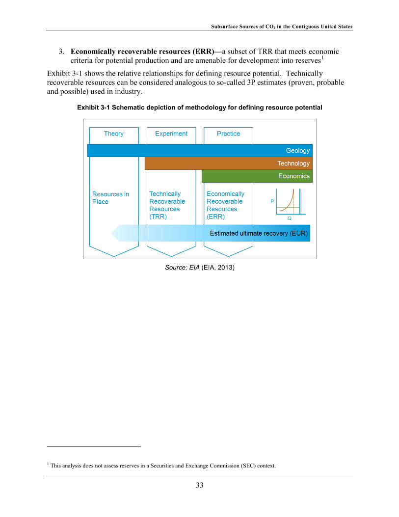
Subsurface Sources of CO2 in the Contiguous United States
3. Economically recoverable resources (ERR)—a subset of TRR that meets economic criteria for potential production and are amenable for development into reserves1
Exhibit 3-1 shows the relative relationships for defining resource potential. Technically recoverable resources can be considered analogous to so-called 3P estimates (proven, probable and possible) used in industry.
Exhibit 3-1 Schematic depiction of methodology for defining resource potential
Source: EIA (EIA, 2013)
1 This analysis does not assess reserves in a Securities and Exchange Commission (SEC) context.
33
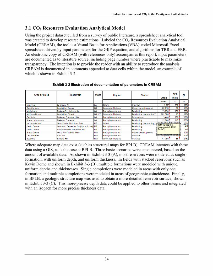
Subsurface Sources of CO2 in the Contiguous United States
3.1 CO2 Resources Evaluation Analytical Model Using the project dataset culled from a survey of public literature, a spreadsheet analytical tool was created to develop resource estimations. Labeled the CO2 Resources Evaluation Analytical Model (CREAM), the tool is a Visual Basic for Applications (VBA)-coded Microsoft Excel spreadsheet driven by input parameters for the GIIP equation, and algorithms for TRR and ERR. An electronic copy of CREAM (with references only) accompanies this report; input parameters are documented as to literature source, including page number where practicable to maximize transparency. The intention is to provide the reader with an ability to reproduce the analysis. CREAM is documented in comments appended to data cells within the model, an example of which is shown in Exhibit 3-2.
Where adequate map data exist (such as structural maps for BPLB), CREAM interacts with these data using a GIS, as is the case at BPLB. Three basic scenarios were encountered, based on the amount of available data. As shown in Exhibit 3-3 (A), most reservoirs were modeled as single formation, with uniform depth, and uniform thickness. In fields with stacked reservoirs such as Kevin Dome and shown in Exhibit 3-3 (B), multiple formations were modeled with unique, uniform depths and thicknesses. Single completions were modeled in areas with only one formation and multiple completions were modeled in areas of geographic coincidence. Finally, in BPLB, a geologic structure map was used to obtain a more-detailed reservoir surface, shown in Exhibit 3-3 (C). This more-precise depth data could be applied to other basins and integrated with an isopach for more precise thickness data.
Exhibit 3-2 Illustration of documentation of parameters in CREAM
34
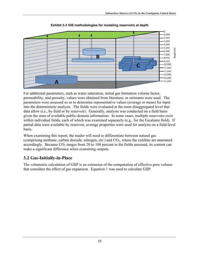
Subsurface Sources of CO2 in the Contiguous United States
Exhibit 3-3 GIS methodologies for modeling reservoirs at depth
For additional parameters, such as water saturation, initial gas formation volume factor, permeability, and porosity, values were obtained from literature, or estimates were used. The parameters were assessed so as to determine representative values (average or mean) for input into the deterministic analysis. The fields were evaluated at the most disaggregated level that data allow (i.e., by field or by reservoir). Generally, analysis was conducted on a field basis given the state of available public-domain information. In some cases, multiple reservoirs exist within individual fields, each of which was examined separately (e.g., for the Escalante field). If partial data were available by reservoir, average properties were used for analysis on a field-level basis.
When examining this report, the reader will need to differentiate between natural gas (comprising methane, carbon dioxide, nitrogen, etc.) and CO2, where the exhibits are annotated accordingly. Because CO2 ranges from 20 to 100 percent in the fields assessed, its content can make a significant difference when examining outputs.
3.2 Gas-Initially-in-Place The volumetric calculation of GIIP is an extension of the computation of effective pore volume that considers the effect of gas expansion. Equation 1 was used to calculate GIIP.
35
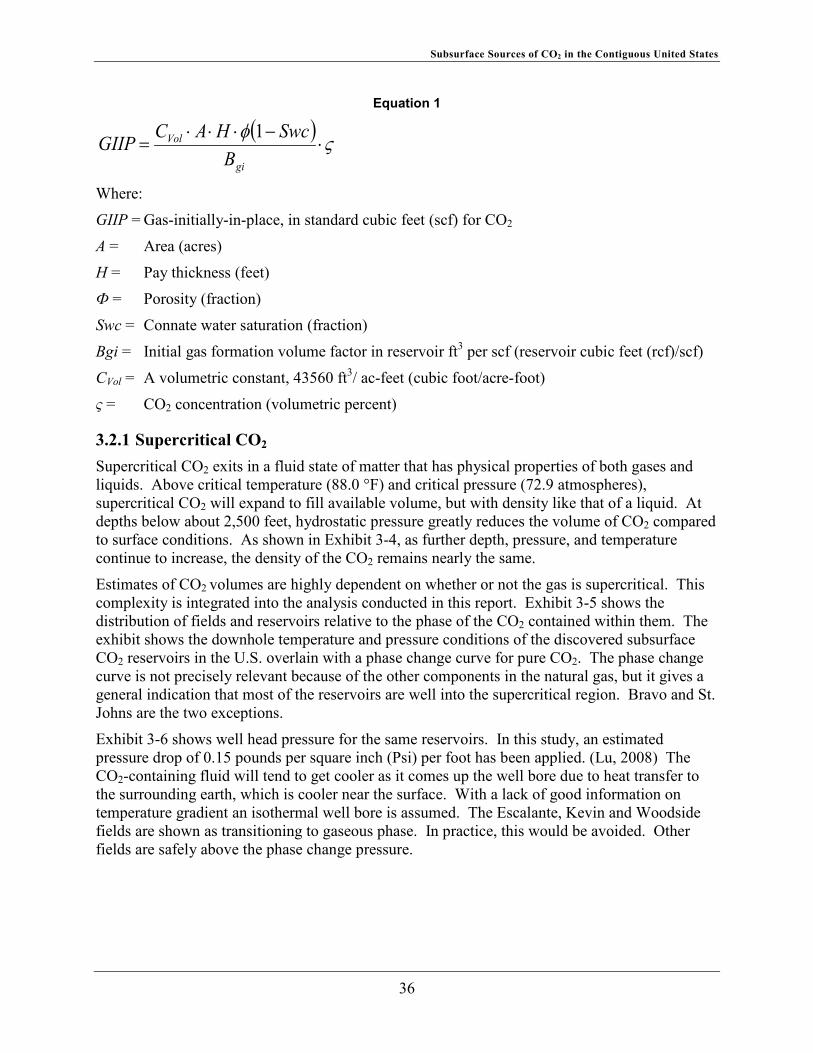
Subsurface Sources of CO2 in the Contiguous United States
Equation 1
gi
Vol
BSwcHACGIIP 1
Where:
GIIP = Gas-initially-in-place, in standard cubic feet (scf) for CO2
A = Area (acres)
H = Pay thickness (feet)
= Porosity (fraction)
Swc = Connate water saturation (fraction)
Bgi = Initial gas formation volume factor in reservoir ft3 per scf (reservoir cubic feet (rcf)/scf)
CVol = A volumetric constant, 43560 ft3/ ac-feet (cubic foot/acre-foot)
= CO2 concentration (volumetric percent)
3.2.1 Supercritical CO2 Supercritical CO2 exits in a fluid state of matter that has physical properties of both gases and liquids. Above critical temperature (88.0 °F) and critical pressure (72.9 atmospheres), supercritical CO2 will expand to fill available volume, but with density like that of a liquid. At depths below about 2,500 feet, hydrostatic pressure greatly reduces the volume of CO2 compared to surface conditions. As shown in Exhibit 3-4, as further depth, pressure, and temperature continue to increase, the density of the CO2 remains nearly the same.
Estimates of CO2 volumes are highly dependent on whether or not the gas is supercritical. This complexity is integrated into the analysis conducted in this report. Exhibit 3-5 shows the distribution of fields and reservoirs relative to the phase of the CO2 contained within them. The exhibit shows the downhole temperature and pressure conditions of the discovered subsurface CO2 reservoirs in the U.S. overlain with a phase change curve for pure CO2. The phase change curve is not precisely relevant because of the other components in the natural gas, but it gives a general indication that most of the reservoirs are well into the supercritical region. Bravo and St. Johns are the two exceptions.
Exhibit 3-6 shows well head pressure for the same reservoirs. In this study, an estimated pressure drop of 0.15 pounds per square inch (Psi) per foot has been applied. (Lu, 2008) The CO2-containing fluid will tend to get cooler as it comes up the well bore due to heat transfer to the surrounding earth, which is cooler near the surface. With a lack of good information on temperature gradient an isothermal well bore is assumed. The Escalante, Kevin and Woodside fields are shown as transitioning to gaseous phase. In practice, this would be avoided. Other fields are safely above the phase change pressure.
36

Subsurface Sources of CO2 in the Contiguous United States
Exhibit 3-4 CO2 (100 percent concentration)
Source: ©2003 BGR (BGR, 2003)
Exhibit 3-5 Downhole pressure, temperature and CO2 phase
Source: NETL
Pressure Temp(bar) (K)
A Bravo 45.0 298B BPLB (basinal) 442.0 377C McElmo Dome 242.7 364D Val Verde 352.3 374E Madden 759.8 441F Jackson Dome 603.3 454G McCallum 159.7 322H Sheep Mountain 149.3 342I Indian Creek 206.8 325J St John's 35.0 304K Doe Canyon 273.0 374L Escalante 75.2 309M Kevin Dome 85.4 306N BPLB (foreland) 476.4 436O BPLB (highland) 523.7 448P Gordon Creek 430.3 362Q Woodside 112.2 312R Oakdale 192.4 355
FormationLabel
37
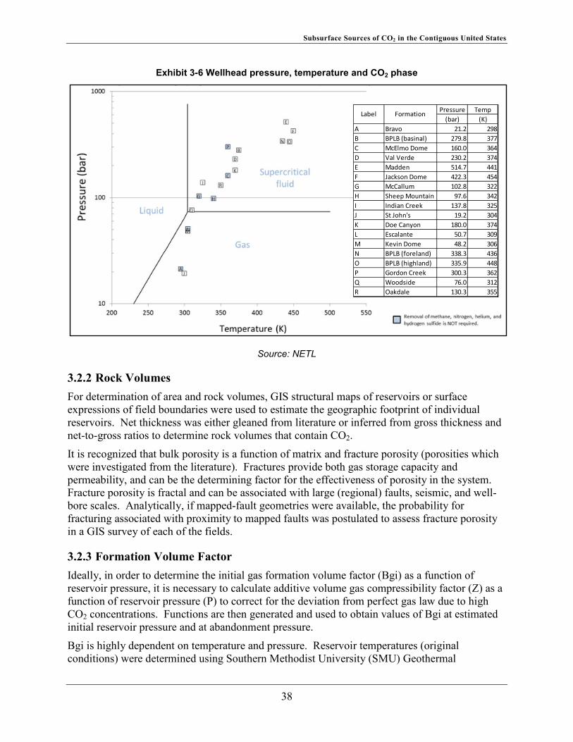
Subsurface Sources of CO2 in the Contiguous United States
Exhibit 3-6 Wellhead pressure, temperature and CO2 phase
Source: NETL
3.2.2 Rock Volumes For determination of area and rock volumes, GIS structural maps of reservoirs or surface expressions of field boundaries were used to estimate the geographic footprint of individual reservoirs. Net thickness was either gleaned from literature or inferred from gross thickness and net-to-gross ratios to determine rock volumes that contain CO2.
It is recognized that bulk porosity is a function of matrix and fracture porosity (porosities which were investigated from the literature). Fractures provide both gas storage capacity and permeability, and can be the determining factor for the effectiveness of porosity in the system. Fracture porosity is fractal and can be associated with large (regional) faults, seismic, and well-bore scales. Analytically, if mapped-fault geometries were available, the probability for fracturing associated with proximity to mapped faults was postulated to assess fracture porosity in a GIS survey of each of the fields.
3.2.3 Formation Volume Factor Ideally, in order to determine the initial gas formation volume factor (Bgi) as a function of reservoir pressure, it is necessary to calculate additive volume gas compressibility factor (Z) as a function of reservoir pressure (P) to correct for the deviation from perfect gas law due to high CO2 concentrations. Functions are then generated and used to obtain values of Bgi at estimated initial reservoir pressure and at abandonment pressure.
Bgi is highly dependent on temperature and pressure. Reservoir temperatures (original conditions) were determined using Southern Methodist University (SMU) Geothermal
Pressure Temp(bar) (K)
A Bravo 21.2 298B BPLB (basinal) 279.8 377C McElmo Dome 160.0 364D Val Verde 230.2 374E Madden 514.7 441F Jackson Dome 422.3 454G McCallum 102.8 322H Sheep Mountain 97.6 342I Indian Creek 137.8 325J St John's 19.2 304K Doe Canyon 180.0 374L Escalante 50.7 309M Kevin Dome 48.2 306N BPLB (foreland) 338.3 436O BPLB (highland) 335.9 448P Gordon Creek 300.3 362Q Woodside 76.0 312R Oakdale 130.3 355
Label Formation
38
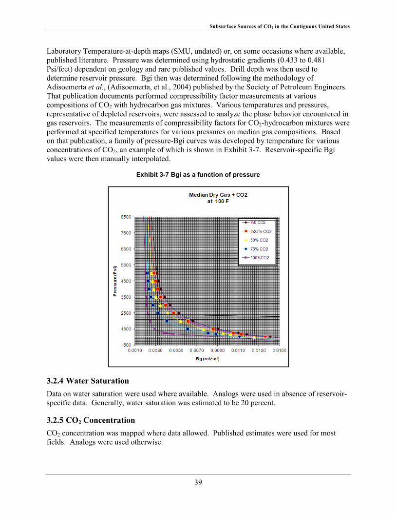
Subsurface Sources of CO2 in the Contiguous United States
Laboratory Temperature-at-depth maps (SMU, undated) or, on some occasions where available, published literature. Pressure was determined using hydrostatic gradients (0.433 to 0.481 Psi/feet) dependent on geology and rare published values. Drill depth was then used to determine reservoir pressure. Bgi then was determined following the methodology of Adisoemerta et al., (Adisoemerta, et al., 2004) published by the Society of Petroleum Engineers. That publication documents performed compressibility factor measurements at various compositions of CO2 with hydrocarbon gas mixtures. Various temperatures and pressures, representative of depleted reservoirs, were assessed to analyze the phase behavior encountered in gas reservoirs. The measurements of compressibility factors for CO2-hydrocarbon mixtures were performed at specified temperatures for various pressures on median gas compositions. Based on that publication, a family of pressure-Bgi curves was developed by temperature for various concentrations of CO2, an example of which is shown in Exhibit 3-7. Reservoir-specific Bgi values were then manually interpolated.
Exhibit 3-7 Bgi as a function of pressure
3.2.4 Water Saturation Data on water saturation were used where available. Analogs were used in absence of reservoir-specific data. Generally, water saturation was estimated to be 20 percent.
3.2.5 CO2 Concentration CO2 concentration was mapped where data allowed. Published estimates were used for most fields. Analogs were used otherwise.
39

Subsurface Sources of CO2 in the Contiguous United States
3.2.6 GIIP Calibration and Estimation Once the parameters were established in CREAM, computer code was developed to calculate the GIIP. GIIP was calculated by formation according to spatial distribution where data were available. The Tab “CREAM_GIIP” presents the data and calculated values.
Fields were examined at the most disaggregated level of information available for the fields. They were run by reservoir where data were obtainable (as in the case of Escalante field) or as a series of polygons where sufficient map data existed to overlay them (e.g., BPLB) to determine intersections comprising discrete GIS polygons. Otherwise, fields were examined as a single reservoir. Ideally, it is beneficial to disaggregated fields at the highest level; unfortunately, these data are not generally available in the public domain. In Appendix A2, Exhibit A2-1 shows the GIIP by field, or respective reservoir where data are available. The fields in Exhibit A2-1 are ordered alphabetically by state as they were input into CREAM.
3.3 Technically Recoverable Resources Technically Recoverable Resources, as a subset of GIIP, were estimated as the next step. TRR is directly influenced by permeability, which can differ among lithologies and depositional environments. A Recovery Factor (RF) was determined, which represents the portion of GIIP that can be technically recovered, where the RF is multiplied against the GIIP to determine TRR. Recovery Factors are generally assumed to be 70 percent and commonly range from 60 to 80 percent. They are adjusted by reservoir in consideration of its geological context.
Recovery factors for each field or reservoir are based on using literature (e.g., Zimmerman, (Zimmerman, 1979) and ETSAP (ETSAP, 2010)) and Enegis’ prior experience. Enegis has conducted, in studies elsewhere, comparisons of Estimated Ultimate Recovery (EUR) to in-place resources and in consideration of connectivity and reservoir rock type (i.e., behavior as a function of lithologic type and in consideration of naturally fracturing, where connectivity can be higher leading to increased technical recovery). In addition, the International Energy Agency (IEA) provides storage coefficients for CO2 (which, in turn, are derived from parameters including relative permeability, vertical to horizontal permeability, anisotropy and injectability) for various lithologies. (IEA, 2009) This work shows that dolomites have the highest coefficients flowed by clastics and limestones.
An important consideration in resource development, which was included in TRR, is that of accessible resources (areas where drilling is able to occur as a function of leasing stipulations) determined using generalized results from the Energy Policy and Conservation Act inventory.
(BLM, 2011) Accessible resources generally range from 20 to 95 percent of TRR. An example of accessible resources determination is shown in Exhibit 3-8, which displays BPLB basinal,
foreland, and highland areas that were estimated to have Access Factors (AF) of 85, 80, and 30 percent accessible, respectively.
Equation 2 shows the relationship between GIIP, RF and AF to determine TRR.
40
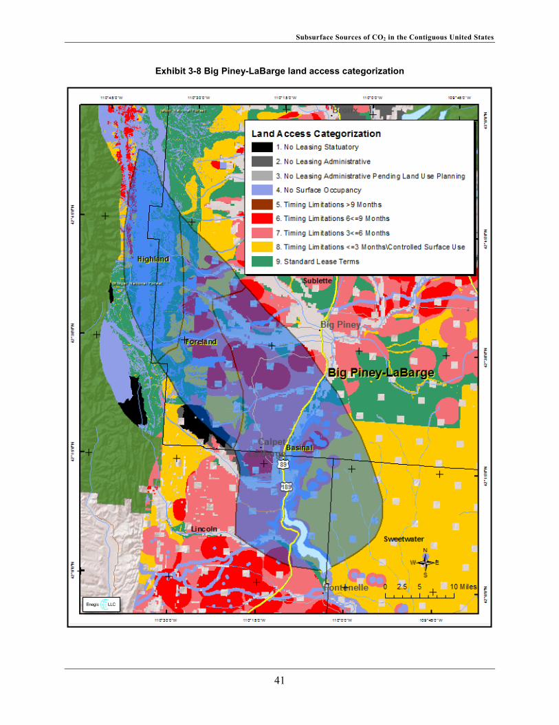
Subsurface Sources of CO2 in the Contiguous United States
Exhibit 3-8 Big Piney-LaBarge land access categorization
41
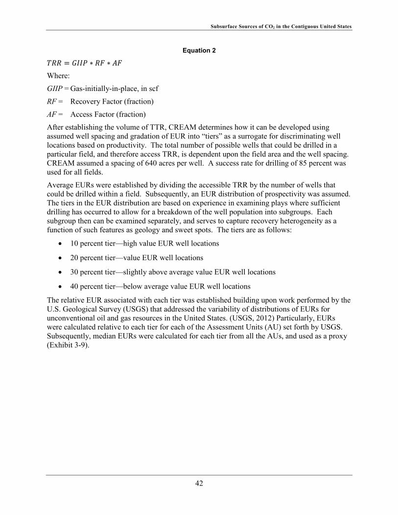
Subsurface Sources of CO2 in the Contiguous United States
Equation 2
= Where:
GIIP = Gas-initially-in-place, in scf
RF = Recovery Factor (fraction)
AF = Access Factor (fraction)
After establishing the volume of TTR, CREAM determines how it can be developed using assumed well spacing and gradation of EUR into “tiers” as a surrogate for discriminating well locations based on productivity. The total number of possible wells that could be drilled in a particular field, and therefore access TRR, is dependent upon the field area and the well spacing. CREAM assumed a spacing of 640 acres per well. A success rate for drilling of 85 percent was used for all fields.
Average EURs were established by dividing the accessible TRR by the number of wells that could be drilled within a field. Subsequently, an EUR distribution of prospectivity was assumed. The tiers in the EUR distribution are based on experience in examining plays where sufficient drilling has occurred to allow for a breakdown of the well population into subgroups. Each subgroup then can be examined separately, and serves to capture recovery heterogeneity as a function of such features as geology and sweet spots. The tiers are as follows:
10 percent tier—high value EUR well locations
20 percent tier—value EUR well locations
30 percent tier—slightly above average value EUR well locations
40 percent tier—below average value EUR well locations
The relative EUR associated with each tier was established building upon work performed by the U.S. Geological Survey (USGS) that addressed the variability of distributions of EURs for unconventional oil and gas resources in the United States. (USGS, 2012) Particularly, EURs were calculated relative to each tier for each of the Assessment Units (AU) set forth by USGS. Subsequently, median EURs were calculated for each tier from all the AUs, and used as a proxy (Exhibit 3-9).
42
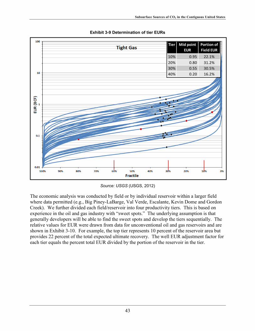
Subsurface Sources of CO2 in the Contiguous United States
Exhibit 3-9 Determination of tier EURs
Source: USGS (USGS, 2012)
The economic analysis was conducted by field or by individual reservoir within a larger field where data permitted (e.g., Big Piney-LaBarge, Val Verde, Escalante, Kevin Dome and Gordon Creek). We further divided each field/reservoir into four productivity tiers. This is based on experience in the oil and gas industry with “sweet spots.” The underlying assumption is that generally developers will be able to find the sweet spots and develop the tiers sequentially. The relative values for EUR were drawn from data for unconventional oil and gas reservoirs and are shown in Exhibit 3-10. For example, the top tier represents 10 percent of the reservoir area but provides 22 percent of the total expected ultimate recovery. The well EUR adjustment factor for each tier equals the percent total EUR divided by the portion of the reservoir in the tier.
Tier Mid point EUR
Portion of Field EUR
10% 0.95 22.1%20% 0.80 31.2%30% 0.55 30.5%40% 0.20 16.2%
43
Subsurface Sources of CO2 in the Contiguous United States
Exhibit 3-10 Factors applied to model tiers of well productivity
Tier Portion of reservoir
% of total EUR
Well EUR adjustment
factor
1st 10 22 2.20
2nd 20 31 1.55
3rd 30 31 1.03
4th 40 16 0.41
Equation 3 is applied to estimated CO2 production per well (PT).
Equation 3
PT = (GR / AR) * SF * EF * FT
Where
PT – production per well for the tier (Tcf/well over a 30-year life)
GR - GIIP for the reservoir (Tcf)
AR - Area of the reservoir (acres)
SF - Well spacing for the field (acres per well)
EF - Estimated ultimate recovery for the field (% CO2 IIP)
FT - Well EUR adjustment factor for the tier (Exhibit 3-10)
In CREAM, the TRR parameters and results are shown on the Tab “CREAM_TRR.” In Appendix A2, shows the TRR by field, which are ordered alphabetically by state as they were input into CREAM.
3.4 Economically Recoverable Resources Economically Recoverable Resources, as a subset of TRR, are estimated by determining project economics based upon estimated drilling, completion, processing, and ancillary costs. Standardized costs were developed, but applied according to factors such as the depth of the reservoir, topography, geographic location, and CO2 price. CREAM uses a net present value (NPV) analysis to discriminate resources as economic or uneconomic. NETL indicated that the CO2 price to be used as $20/tonne, or $1.06/thousand cubic feet (Mcf). This price is considered to occur at the lease-line and does not consider pipeline costs for transportation to market.
44

Subsurface Sources of CO2 in the Contiguous United States
CREAM runs the analysis per tier by reservoir, reading reservoir parameters and posting to a worksheet NPV analysis, which cycles through to return the NPV and associated ERR values. In the NPV analysis, the first year (year zero) is considered to be for lease acquisition and drilling, with production scheduled over 30 years using 6 percent annual decline. CO2 revenue is posted as a function of CO2 price and production volume. A royalty was established at an assumed rate of 12.5 percent, which is that charged on federal lands.
Drilling capital expense (CAPEX) is determined as a function of drill depth based on regional $/foot data from the Energy Information Administration (EIA). (EIA, 2013) Drilling success rate, assumed to be 85 percent, established a 15-percent dry-hole burden. CAPEX costs were also considered for gathering lines based on Interstate Natural Gas Association of America (INGAA) (INGAA, 2010) (INGAA, 2011) and EIA data, (EIA, 2012) as well as dehydration costs based on Environmental Protection Agency (EPA) (EPA, 2008) data. Operating expense (OPEX) costs were considered for dehydration based on EPA data, (EPA, 2008) as well as monthly well and lease costs, such as electricity and maintenance.
Compression costs are significant in CO2 field development. Suction (inlet) compressor pressures are estimated at original reservoir pressure, reservoir pressure decline, head pressure loss and gathering line loss. Based on research as documented in CREAM, a pressure was established for each reservoir. Reservoir pressure declines are considered as a function of EUR depletion over the productive life of a reservoir based on the portion of the EUR extracted relative to the total resource in a given productive year. Head pressure loss is calculated by considering the depth of the formation and a gradient of 0.15 Psi/foot. (Lu, 2008) Gathering line loss is estimated to be 250 Psi based on experience. (Fox, 2013) For reservoirs at high pressures, a suction pressure of 600 Psi was assumed as the optimum for removing (“knocking out”) water from the CO2. (Fox, 2013) As a simplification, for low pressure reservoirs, a maximum initial suction of 50 Psi was assumed. In addition, if the field undergoes processing for non-CO2 gases, e.g., as occurs at BPLB, a suction pressure of 50 Psi is assumed. (Fox, 2013) (Denbury, July 2013) The pipeline pressure requirement is 2,200 Psi. (INGAA, 2010) Compression costs are calculated at a rate of 0.000237 $/Mcf/deltaPsi based on Summers, which calculated a cost of $9.95/tonne assuming an inlet pressure of 1.6 bars (see Equation ). (Summers, 2013, in publication)
45
Subsurface Sources of CO2 in the Contiguous United States
Equation 4
0.000237 = $9.95/ 0.053 2 /
Where:
= Outlet-inlet pressure The economic impact of other co-mingled natural gases is considered. If methane is present, it is assumed to be produced at $5.00 per Mcf at a 10 percent margin. The margin was set to accommodate increased costs associated with separation of methane. $5.00 per Mcf was chosen based on the long-term projections of prices by EIA. (EIA, 2013) If N2 is present in a field, CREAM considers concentrations greater than 4 percent beyond pipeline specifications and scrubs it at a cost of $0.41 to $0.90/Mcf (levelized based on costs presented in Mitariten (Mitaritan, 2009)) dependent upon well production rates. If H2S is present, CREAM first scrubs to a pipeline specification of 35 parts per million (ppm) at a cost of $6.75/Mcf (levelized based on costs presented in Cline et al. (Cline, 2012)). It was confirmed that sulfur produced at the Lost Cabin facility, Madden field, is currently being sold into the local fertilizer market. (ConocoPhillips, undated) CREAM assumes that sulfur produced at Jackson Dome will likewise be sold at a price of $142 per ton. (Feytis, 2012)
Earnings before taxes (EBT) is established as a cash flow sum by year over the presumed 30-year life of production. Taxes are assessed at a 35 percent rate to include federal and state income, severance, and ad valorem taxes. A discount rate of 12 percent is assumed.
The presence of methane or marketable sulfur can enhance the economics of development of a deposit, although, especially for methane, the more fundamental question can be whether the deposit is being developed for methane itself with CO2 development as ancillary (as in the case of the Madden field). Further, if the sulfur is not sold, its processing and handling can become a significant cost item. If sulfur is not sold, CREAM assumes that reinjection will cost 75 percent of sulfur processing costs. Helium was also considered in the economic analysis for reservoirs where its content was 0.2 percent of greater. The cost for helium production is based on Bureau of Land Management (BLM) (BLM, 2013) and a generalized helium price ($125/Mcf) on Washington Post. (Washington Post, 2012)
CREAM assesses NPV by tier (10, 20, 30, and 40 percent). Reservoir NPV, and thereby ERR, are determined by the dry hole burden times the number of wells, times the EUR (by tier), times the CO2 concentration. CREAM assumes that the drilling that occurs in the fields is selective, i.e., it assumes that there is “learning by doing” where industry, by knowledge and insight, avoids drilling negative NPV wells. The results are calculated in the spreadsheet via a macro and then posted to the CREAM results section. (See the Tabs “CREAM_ERR_R” where all NPVs are posted and “CREAM_ERR_S” where positive NPVs values only are posted. The positive NPVs are assumed to be what industry is able to focus upon given learning feedback.) In Appendix A2, Exhibit A2-3 and Exhibit A2-4 show the ERR for CO2 by field (ordered alphabetically by state as they were input into CREAM). Finally, estimates of already produced CO2 in each of the fields were determined (Exhibit 3-11) and subtracted from ERR to determine remaining or net ERR.
46
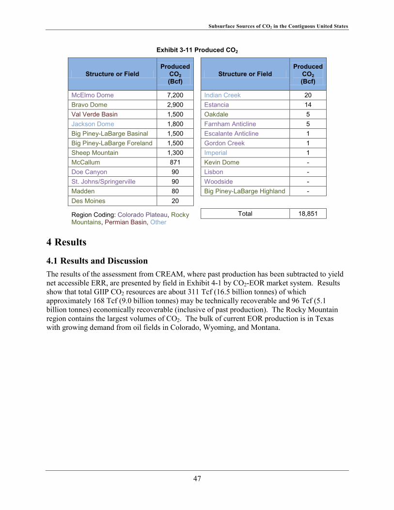
Subsurface Sources of CO2 in the Contiguous United States
Exhibit 3-11 Produced CO2
Structure or Field Produced
CO2 (Bcf)
Structure or Field Produced
CO2 (Bcf)
McElmo Dome 7,200 Indian Creek 20 Bravo Dome 2,900 Estancia 14 Val Verde Basin 1,500 Oakdale 5 Jackson Dome 1,800 Farnham Anticline 5 Big Piney-LaBarge Basinal 1,500 Escalante Anticline 1 Big Piney-LaBarge Foreland 1,500 Gordon Creek 1 Sheep Mountain 1,300 Imperial 1 McCallum 871 Kevin Dome - Doe Canyon 90 Lisbon - St. Johns/Springerville 90 Woodside - Madden 80 Big Piney-LaBarge Highland - Des Moines 20
Region Coding: Colorado Plateau, Rocky Mountains, Permian Basin, Other
Total 18,851
4 Results
4.1 Results and Discussion The results of the assessment from CREAM, where past production has been subtracted to yield net accessible ERR, are presented by field in Exhibit 4-1 by CO2-EOR market system. Results show that total GIIP CO2 resources are about 311 Tcf (16.5 billion tonnes) of which approximately 168 Tcf (9.0 billion tonnes) may be technically recoverable and 96 Tcf (5.1 billion tonnes) economically recoverable (inclusive of past production). The Rocky Mountain region contains the largest volumes of CO2. The bulk of current EOR production is in Texas with growing demand from oil fields in Colorado, Wyoming, and Montana.
47
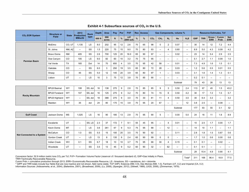
Subsurface Sources of CO2 in the Contiguous United States
Exhibit 4-1 Subsurface sources of CO2 in the U.S.
CO2 EOR System Structure or Field State
2013 Production
MMscfd
Rock type
Depth Area Pay Por FVF Rec Access Gas Components, volume % Resource Estimates, Tcf
000 ft 000 acres ft % rcf/
(000 scf) % % CO2 CH4 N2 He H2S GIIP TRR Gross ERR
Cumm Prdn
Net ERR
Permian Basin
McElmo CO, UT 1,135 LS 8.0 202 95 12 2.6 70 65 98 0 2 0.07 -- 30 14 12 7.2 4.4
St. Johns NM, AZ -- SS 1.5 220 75 15 9.0 70 80 93 -- 4 0.60 -- 8.9 5.0 4.3 0.09 4.2
Bravo Dome NM 405 SS 2.6 700 125 20 16.0 65 90 97 -- -- 0.02 -- 23 14 5.4 2.9 2.5
Doe Canyon CO 105 LS 9.0 82 60 10 3.2 70 75 95 -- -- -- -- 5.1 2.7 1.1 0.09 1.0
Val Verde TX 165 Dol 14 70 650 4 3.5 70 95 42 58 -- 0.01 -- 7.3 4.9 1.6 1.5 0.1
Oakdale CO -- SS 6.0 3 250 19 3.5 65 80 72 28 -- 0.03 -- 1.2 0.6 0.5 0.01 0.5
Sheep CO 45 SS 5.0 12 145 20 3.9 65 80 97 1 -- 0.03 -- 3.1 1.6 1.4 1.3 0.1
Lisbon UT -- LS 10 3 75 12 3.8 70 85 90 -- -- -- -- 0.2 0.1 -- -- --
Subtotal 79 43 26 13 13
Rocky Mountain
BPLB Basinal WY 108 SS, dol 16 138 275 9 2.8 70 85 85 9 3 0.50 2.4 113 67 45 1.5 43.2
BPLB Foreland WY 107 SS, dol 16 125 275 9 3.2 70 80 74 15 6 0.50 4.2 30 17 7.2 1.5 5.7
BPLB Highland WY -- SS, dol 18 388 275 9 3.0 70 30 81 11 4 0.50 3.0 30 6.4 3.2 -- 3.2
Madden WY 35 dol 24 80 175 15 3.8 70 95 20 67 -- -- 12 3.8 2.5 -- 0.08 --
Subtotal 177 93 55 3.1 52
Gulf Coast Jackson Dome MS 1,025 LS 16 90 185 13 2.8 70 95 90 5 -- 0.00 5.0 24 16 11 1.8 8.9
Not Connected to a System
Escalante UT -- SS, LS 2.3 37 172 7 9.1 55 45 95 -- 4 0.01 -- 10 2.5 1.7 0.00 1.7
Kevin Dome MT -- LS 3.6 261 67 9 5.3 75 95 88 -- 12 -- -- 14 10 1.1 -- 1.1
McCallum CO 1.0 SS 5.5 15 100 20 3.5 70 90 92 -- -- 0.11 -- 2.8 1.8 1.5 0.87 0.6
Gordon Creek UT -- LS 13 8 135 9 2.4 65 90 99 0 0 - -- 1.7 1.0 0.6 0.00 0.6
Indian Creek WV 0.1 SS 6.7 18 10 10 3.7 70 95 66 30 4 0.15 -- 0.1 0.1 -- 0.02 --
Woodside UT -- SS 3.5 13 45 9 5.2 60 90 32 -- 62 -- -- 0.1 0.1 -- -- --
Subtotal 29 15.4 4.9 0.90 4.1
Conversion factor: 52.9 million metric tons CO2 per Tcf, FVF= Formation Volume Factor (reservoir cf / thousand standard cf), GIIP=Gas Initially in Place, TRR=Technically Recoverable Resource, Cumm Prdn = cumulative production through 2013, ERR= Economically Recoverable Resource, LS - limestone, SS = sandstone, dol = dolomite
Total* 311 168 96.4 18.9 77.5
* GIPP and TRR totals include four fields that are now inactive and not shown, field name (state, TCF GIIP): Estancia (NM, 0.9), Des Moines (NM, 1.0), Farnham (UT, 0.2) and Imperial (CA, 0.2) Information Sources: (Adisoemerta, et al., 2004), (Ballentine, 2001), (Broadhead, 2009), (Lu, 2008), (Spangler, 2012), (Stilwell, 1989), (UGS, 2008), (Zimmerman, 1979).
48
Subsurface Sources of CO2 in the Contiguous United States
The BPLB, in the Greater Green River basin of Wyoming, is the largest single discovered CO2 resource in the U.S., with an estimated GIIP of 173 Tcf in aggregate, or 56 percent of the discovered resource base. The basinal portion of BPLB has an estimated remaining ERR of 43.2 Tcf. BPLB was originally developed for its methane content, but is experiencing significant increases in the use of its CO2 in EOR.
Other fields with 2 Tcf or more of gross ERR comprise McElmo Dome in Colorado and Utah (11.6 Tcf, currently producing and expanding), Jackson Dome in Mississippi (10.7 Tcf currently producing and expanding), BPLB foreland area in Wyoming (7.2 Tcf and currently producing), the Bravo Dome in New Mexico (5.4 Tcf and currently productive), St. Johns/Springerville in New Mexico and Arizona (4.3 Tcf under development), BPLB highland area in Wyoming (3.2 Tcf), and the Val Verde Basin (1.6 Tcf currently producing and expanding). McElmo Dome field, a workhorse for CO2 supply, producing about 1.1 Bcf/d, is estimated in CREAM to be past peak production and is modeled as having about 4.4 Tcf of ERR remaining, although available data in the public domain lead to uncertain estimates. Fields in the Val Verde basin in Texas, located close to EOR developments, have been exploited for CO2. CREAM is able to discriminate the seven fields located in the Val Verde basin only by CO2 content, and compute an aggregate ERR estimate of about 0.1 Tcf in aggregate left to produce in ERR.
Other noteworthy fields include, Escalante Anticline in Utah (1.7 Tcf undeveloped and largely inaccessible), Kevin Dome in Montana (1.1 Tcf producing), and the Doe Canyon field (1.1 TCF under development), located near McElmo field. CREAM estimates are higher than Kinder-Morgan CO2’s indication adding 750 Bcf of reserves. (Bradley, 2011) The McCallum field in Colorado is currently producing and has about 627 Bcf of ERR. The Gordon Creek field in Utah is in development and is estimated to contain about 604 Bcf of ERR.
Sheep Mountain field, a productive field since its discovery in the 1970s, is modeled as being nearly depleted. The Madden field, which has been developed for its methane but contains 20 percent CO2, has about 2.5 Tcf of CO2 TRR (the fact that CREAM is showing no CO2 ERR is a reflection of the fact that it would not be economically viable to develop the field for its CO2 resources alone). At Madden, the Lost Cabin natural gas processing facility is being expanded to capture the CO2 (up to 60 MMcfd) for use in EOR in Wyoming and Montana. (Condon, 2011) The Des Moines field, in New Mexico, is proximal to Bravo Dome and has about 600 Bcf of TRR. The remaining eight fields examined are small, on the order of less than 500 Bcf each (and about 2 Tcf in aggregate) and are less likely to contribute to CO2 supply.
The spreadsheet tool, CREAM, was exercised to assess the sensitivity of the ERR estimates to the assumed field gate price for CO2. Exhibit 4-2 shows the results in terms of net ERR, that is the gross ERR minus cumulative production. From the reference value of $1.06/Mscf (20 $/mtCO2), a 25% drop in CO2 price causes a 73% drop in net ERR; a 25% increase in CO2 price causes a 35% increase in net ERR. None of the fields are economic at $0.53/Mscf. Bravo, Doe Canyon, Val Verde and Kevin Dome all realize significant increase in net ERR going from $1.06 /Mscf to $1.32/Mscf. The reason for this is that tiers within the reservoir become economic with higher revenue.
49
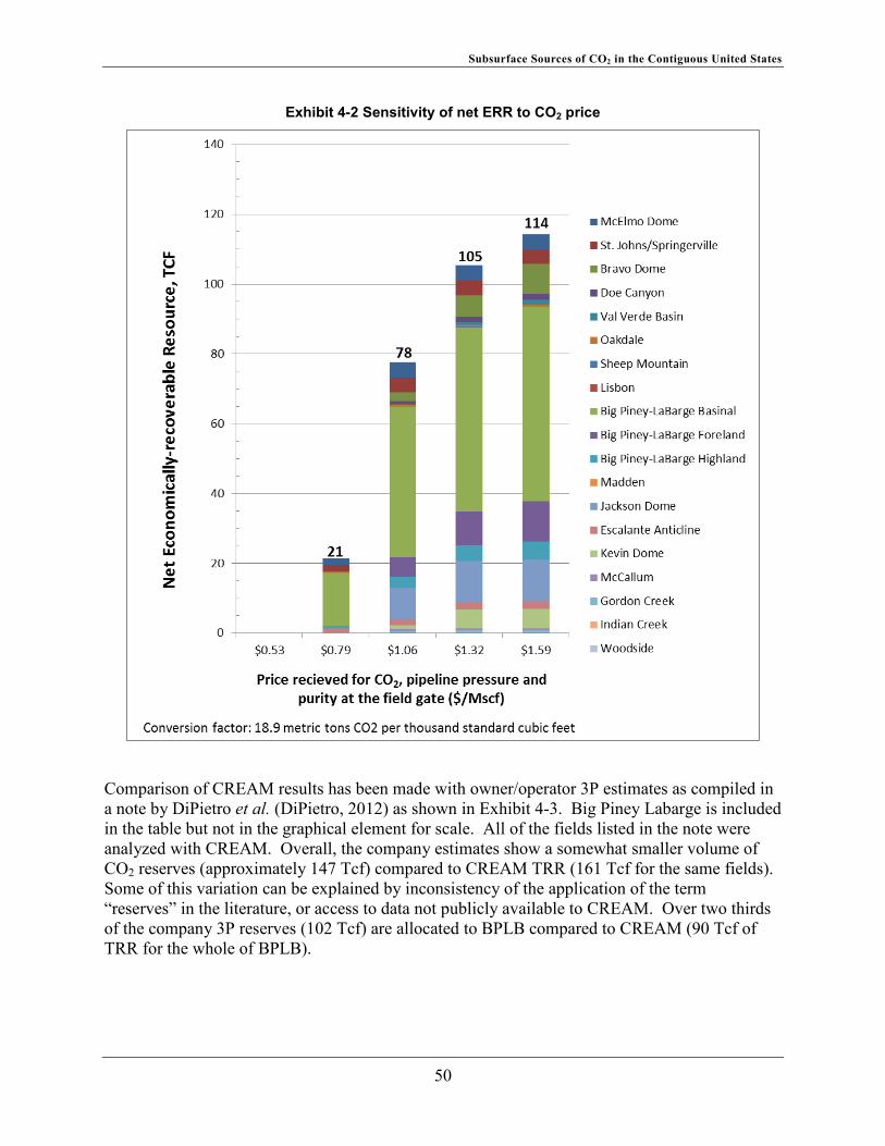
Subsurface Sources of CO2 in the Contiguous United States
Exhibit 4-2 Sensitivity of net ERR to CO2 price
Comparison of CREAM results has been made with owner/operator 3P estimates as compiled in a note by DiPietro et al. (DiPietro, 2012) as shown in Exhibit 4-3. Big Piney Labarge is included in the table but not in the graphical element for scale. All of the fields listed in the note were analyzed with CREAM. Overall, the company estimates show a somewhat smaller volume of CO2 reserves (approximately 147 Tcf) compared to CREAM TRR (161 Tcf for the same fields). Some of this variation can be explained by inconsistency of the application of the term “reserves” in the literature, or access to data not publicly available to CREAM. Over two thirds of the company 3P reserves (102 Tcf) are allocated to BPLB compared to CREAM (90 Tcf of TRR for the whole of BPLB).
50
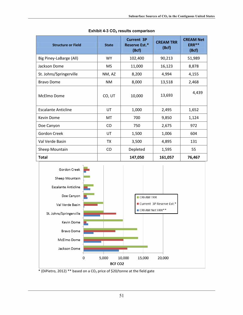
Subsurface Sources of CO2 in the Contiguous United States
Exhibit 4-3 CO2 results comparison
Structure or Field State Current 3P Reserve Est.*
(Bcf)
CREAM TRR (Bcf)
CREAM Net ERR** (Bcf)
Big Piney-‐LaBarge (All) WY 102,400 90,213 51,989
Jackson Dome MS 11,000 16,123 8,878
St. Johns/Springerville NM, AZ 8,200 4,994 4,155
Bravo Dome NM 8,000 13,518 2,468
McElmo Dome CO, UT 10,000
13,693
4,439
Escalante Anticline UT 1,000 2,495 1,652
Kevin Dome MT 700 9,850 1,124
Doe Canyon CO 750 2,675 972
Gordon Creek UT 1,500 1,006 604
Val Verde Basin TX 3,500 4,895 131
Sheep Mountain CO Depleted 1,595 55
Total 147,050 161,057 76,467
* (DiPietro, 2012) ** based on a CO2 price of $20/tonne at the field gate
51
Subsurface Sources of CO2 in the Contiguous United States
In Bravo Dome, CREAM is showing less than twice as much TRR as in 3P estimates but a significantly lower ERR volume. At Jackson Dome and Bravo dome, CREAM estimates bracket 3P estimates. At St. Johns/Springerville CREAM estimates are about half of 3P estimates. At Escalante Anticline, CREAM is depicting almost two and a half times as much TRR (2.5 Tcf) and over one a half times as much ERR (1.6 Tcf) as company estimates show (1 Tcf). Other fields of note are Doe Canyon, where CREAM ERR is consistent with 3P estimates (and announced company plans for development (Bradley, 2011)) and Sheep Mountain, which is considered to be depleted and where CREAM confirms negligible remaining ERR.
Overall, of the TRR assessed in this study, about 58 percent may yet be economically recoverable. The Big Piney-LaBarge field in Wyoming contains an estimated remaining ERR of 52 Tcf, 67 percent of the total for the United States. The remaining ERR in reservoirs that feed into the Permian Basin and Gulf Coast is on the order of 10-20 years of supply. The technically recoverable resource (TRR) in the Permian Basin and Gulf Coast is on the order of 30 years of supply. The ERR at LaBarge contains an estimated 260 Bcf of helium, while the ERR at St Johns/Springerville may contain 25 Bcf of helium.
4.2 Uncertainty There are other areas of uncertainty in the estimates for GIIP, TRR and ERR. For example, we were not able to find unique maps for Bravo or Jackson Dome. The cost and performance of helium capture systems and other gas processing operations are held as proprietary. We do not have production well models or systems analyses of gas processing systems to predict CO2 compressor inlet pressure at each field. The TRR recovery factors (%GIIP recoverable) are based on literature research and the expertise of the authors rather than measurements of reservoir permeability. Well spacing is generically applied. NETL is undertaking efforts to address these areas of uncertainty and others and plans to publish an updated version of its working paper.
Another source of uncertainty in the resource estimate is the potential for discovery of new CO2 field(s). Accordingly, NETL is undertaking a parallel effort to identify and assess leads for undiscovered CO2 resources in the United States. That study looks more closely at the geology and tectonics of the discovered CO2 reservoirs and the sequence of trap formation and CO2 emplacement. The study then explores five areas for possible undiscovered leads within the geologic trends where the discovered reservoirs are found. A companion NETL document contains the analysis of undiscovered CO2 resources.
52
Subsurface Sources of CO2 in the Contiguous United States
5 References Cited
Adisoemerta, P.S. and S.M. Frailey, and A.S., Lawal. 2004. Measured Z Factor of CO2--Dry Gas/Wet Gas/Gas Condensate for CO2 Storage in Depleted Reservoirs, Society of Petroleum Engineers Paper 89466. s.l. : Society of Petroleum Engineers, 2004.
Avary, K. L. 1996. Play Sts: The Lower Silurian Tuscarora Sandstone Fractured Anticlinal Play. The Atlas of Major Appalachian Gas Plays: West Virginia Geological and Economic Survey. 1996, Vols. V-25, pp. 151-155.
Ballentine, C., M. Schoell, D. Coleman, and B. Calm. 2001. 300-Myr-old magmatic CO2 in natural gas reservoirs on the west Texas Permian basin. Nature. 2001, Vol. 409, p. 327.
BGR. 2003. What is CCS? BGR. [Online] 2003. [Cited: February 11, 2013.] http://www.bgr.bund.de/EN/Themen/CO2Speicherung/FAQ/faq_node_en.html#doc1559834bodyText1.
BLM. 2011. EPCA Phase III Inventory. [Online] 2011. [Cited: February 11, 2013.] http://www.blm.gov/wo/st/en/prog/energy/oil_and_gas/EPCA_III.html.
—. 2013. Federal Helium Program Frequently Asked Questions, What are the BLM’s prices for crude helium? What will the helium prices be next year? [Online] 2013. [Cited: May 11, 2013.] http://www.blm.gov/nm/st/en/prog/energy/helium/federal_helium_program/federal_helium_program.html.
—. 2002. Mineral Potential Report: Bureau of Land Management, Price, Utah Field Office. 2002.
Boyce, Richard G. 2009. Unlocking Multiple plays in a Developing Resource. dB, LLC Petroleum Advisors. [Online] Mar 27, 2009. [Cited: Feb 13, 2014.] http://www.slideshare.net/dbseismo/west-texas-overthrust-play.
Bradley, T. and J. Wuerth. 2013. CO2 Kinder Morgan investor presentation. [Online] 2013. [Cited: February 11, 2013.] http://www.-kindermorgan.com/investor/presentations/013013_CO2.pdf .
Bradley, T. 2011. CO2 Kinder Morgan investor presentation. [Online] 2011. [Cited: February 11, 2013.] http://www.kindermorgan.com-/investor/presentations/presentations.cfm?year=2011.
53
Subsurface Sources of CO2 in the Contiguous United States
Broadhead, R. F., M. Mansell and G. Jones. 2009. Carbon Dioxide in New Mexico: Geologic Distribution of Natural Occurrences. s.l. : New Mexico Bureau of Geology and Mineral Resources, Open File Report No. 514, 2009.
Cassidy, M. 2005. Occurrence and Origin of Free Carbon Dioxide Gas Deposits in the Earth's Continental Crust. s.l. : PhD. Dissertation, Dept. of Geosciences, University of Houston, 2005.
Chidsey, T., C., M. Laine, J. Vrona, and D. Strickland. 2007. Covenant Oil Field, Central Utah Thrust Belt: Possible Harbinger of Future Discoveries, American Association of Petroleum Geologists Search and Discovery Article #10130. s.l. : American Association of Petroleum Geologists, 2007.
Cline, C., A. Hoksberg, R. Abry, and A. Janssen. 2012. Biological Process For H2s Removal From Gas Streams. The Shell-Paques/Thiopaq™ Gas Desulfurization Process. [Online] 2012. [Cited: February 11, 2013.] http://www.environmental-expert.com/Files/587/articles/5529/paques6.pdf.
Condon, C. and M. Parker. 2011. Shute Creek Treating Facility Project Updates. [Online] The Wyoming Enhanced Oil Recovery Institute 5th Annual Wyoming CO2 Conference. July 13, 2011. [Cited: February 11, 2013.] http://www.uwyo.edu/eori/_files/co2conference11/clay%20%20exxonmobil%202011%20eori%20presentation%20-%20final.pdf.
ConocoPhillips. undated. Lost Cabin Gas Plant CO2. [Online] undated. [Cited: February 11, 2013.] http://www.uwyo.edu/eori-/_files/co2conference07/brent_lohnes_conocophillips_eori.pdf.
Denbury. 2012. Analyst Day Presentation. [Online] November 2012. [Cited: February 11, 2013.] http://www.denbury.com/files/2012-11%20Analyst%20Meeting%20FINAL_v001_q03n07.pdf.
—. July 2013. Rocky Mountain Activity Update. July 2013. pp. 16-25.
DiPietro, P., P. Balash, and M. Wallace. 2012. A Note on Sources of CO2 Supply for Enhanced-Oil-Recovery Operations. s.l. : Society of Petroleum Engineers Economics & Management, 2012.
54
Subsurface Sources of CO2 in the Contiguous United States
EIA. 2013. AEO2013 Early Release Overview. [Online] 2013. [Cited: February 11, 2013.] http://www.eia.gov/forecasts/aeo/er/index.cfm.
—. 2012. Natural Gas, Data, Number of Producing Gas Wells. [Online] 2012. [Cited: February 11, 2013.] http://www.eia.gov/dnav/ng/ng_prod_wells_s1_a.htm.
—. 2013. Status and outlook for shale gas and tight oil development in the U.S. for Platts – North American Crude Marketing Conference. Houston, TX : U.S. Energy Information Administration, 2013.
EPA. 2008. Methane to Markets, Natural Gas Dehydrator Optimization, IAPG & US EPA Technology Transfer Workshop. [Online] 2008. [Cited: February 11, 2013.] http://www.epa.gov/gasstar/documents/workshops/buenosaires-2008/dehydrator_optimization.pdf.
ETSAP. 2010. Conventional Oil and Gas Technologies. [Online] 2010. [Cited: November 2, 2013.] http://www.iea-etsap.org/web/P01-Conv-Oil&Gas-GS-gct-AD.pdf.
Feytis, A. 2012. Sulfur Prices CFR Tampa drop 15% from 2011 Year End. [Online] 2012. http://www.indmin.com/Article/2995706/Sulphur-prices-CFR-Tampa-drop-15-from-2011-year-end.html.
Fox, C. 2013. Personal communication. 2013.
Gilfillan, S., C. Ballentine, G. Holland, D. Blagburn, B. Sherwood Lollar, S. Stevens, M. Schoell, and M. Cassidy. 2008. The noble gas geochemistry of natural CO2 gas reservoirs from the Colorado Plateau and Rocky Mountain provinces. Geochimica et Cosmochimica Acta. 2008, Vol. 72, 4, pp. 1174-1198.
Gilluly, J. 1929. U.S. Geological Survey. Bulletin 806-C. 1929.
Hamak, J. E., and B. D. Gage. 1992. Analyses of natural gases, 1991: U.S. Bureau of Mines Information Circular IC 9318. 1992. p. 97.
Hamak, J. E., and S. Sigler. 1991. Analyses of natural gases, 1986-1990: U.S. Bureau of Mines Information Circular IC 9301. 1991. p. 315.
55
Subsurface Sources of CO2 in the Contiguous United States
Hare, M., H. Perlich, R. Robinson, M. Shah, and F. Zimmerman. 1978. Sources and Delivery of Carbon Dioxide for Enhanced Oil Recovery. s.l. : US. Department of Energy, Contract No. EX-76-C-01-2515, 1978.
Hester, R. and R. Holland. 1959. Structure of the Puckett Field, Pecos County, Texas, 1959 Val Verde Field Trip Guidebook. 1959.
Holz, M., P. Nance, and R. Finley. 1999. Reduction on Greenhouse Gas Emissions through Underground CO2 Sequestration in Texas Oil and Gas Reservoirs. s.l. : Bureau of Economic Geology, 1999.
IEA. 2009. Greenhouse Gas Program—Development of Storage Coefficients for Carbon Dioxide Storage in Deep Saline Formations, Technical Study Report No. 2009/13, Table 2. 2009.
INGAA. 2010. CCS Transport, Barriers to Widespread Deployment. 2010.
—. 2011. North American Natural Gas Midstream Infrastructure Through 2035: A Secure Energy Future. [Online] 2011. [Cited: February 11, 2013.] http://www.ingaa-.org/File.aspx?id=14911.
Jenden, P.D., D.J. Drazan, and I.R. Kaplan. 1993. Mixing of thermogenic natural gases in northern Appalachian basin. 1993, Vol. 77, pp. 980-998.
Khayyal, T. July 2013. LaBarge/Shute Creek Facility Update. s.l. : The Wyoming Enhanced Oil Recovery Institute, 7th Annual Wyoming CO2 Conference, July 2013. pp. 3-9.
Kinder Morgan CO2. 2013. McElmo Dome. [Online] 2013. [Cited: February 11, 2013.] http://www.kindermorgan-.com/business/co2/supply_mcelmo.cfm.
Lake, J. Nad S. Whittaker. 2006. Occurrences of CO2 within southwest Saskatchewan: Natural analogues to the Weyburn CO2 injection site. Summary of Investigations. Saskatchewan Geological Survey, Misc. Rep. 2006-4.1, 2006, Vol. 1, Paper A-5, p. 14.
Lu, M., and L. D. Connell. 2008. Non-isothermal flow of carbon dioxide in injection wells during geological storage, Figure 1. International Journal of Greenhouse Gas Control 2. 2008. pp. 248-258.
MGS. 1985. Montana Oil & Gas Fields, Figure 2. s.l. : Montana Geological Society Symposium, 1985.
56
Subsurface Sources of CO2 in the Contiguous United States
Mitaritan, M. 2009. Economic N2 Removal, Hydrocarbon Engineering Magazine, 2004 (updated 2009). [Online] 2009. [Cited: February 11, 2013.] http://www.moleculargate.com/nitrogen-rejection-N2-removal/Economic-N2-Removal-Hydrocarbon-Engineering.pdf.
Moore, J. and M. Adams, R. Allis, S. Lutz, and S. Rauzi. Arizona and New Mexico, Second Annual Conference on Carbon Sequestration. 2003. CO2 Mobility in Natural Reservoirs Beneath the Colorado Plateau and Southern Rocky Mountains: An Example from the Springerville-St. Johns Field. [Online] Arizona and New Mexico, Second Annual Conference on Carbon Sequestration. 2003. [Cited: February 11, 2013.] http://geology.utah.gov/emp/co2sequest/pdf/mobility.pdf.
Muffler, P., and D. White. 1968. Origin of CO2 in the Salton Sea Geothermal System, Southeastern California, U.S.A. XXIII International Geological Congress. 1968, Vol. 17, pp. 185-194.
Murrell, Glen, and Phil DiPietro. 2013. North American CO2 Supply and Developments. University of Wyoming. [Online] Dec 11-13, 2013. [Cited: Feb 13, 2013.] http://www.co2conference.net/wp-content/uploads/2013/12/2-Dipietro-CO2-Supply-2013_v7.pdf.
National Academies. 2010. "4 Helium Sourcing and Reserves." Selling the Nation's Helium Reserve. Washington D.C. : The National Academies Press, 2010.
NETL. undated. Natural CO2 Reservoirs on the Colorado Plateau and Southern Rocky Mountains: Candidates for CO2 Sequestration. [Online] undated. [Cited: February 11, 2013.] http://www.netl.doe.gov/publications/proceedings/01/carbon_seq/6a2.pdf.
SMU. undated. Enhanced Geothermal Systems Potential in Google Earth. [Online] undated. [Cited: February 11, 2013.] http://www.google.org/egs/.
Spangler, L. Bowen, D., Talbot, J. 2012. Montana Characterization Study - Comprehensive Report Deliverable Gd30 (Task 15). National Energy Technology Laboratory Infrastructure Meeting : Big Sky Carbon Sequestration Partnership, 2012.
Stevens, S.H., J. M. Pearce, and A. A. J. Rigg. May 15-17, 2001. Natural Analogs for Geologic Storage of CO2: An Integrated Global Research Program. s.l. : U.S. Department of Energy, National Energy Technology Laboratory, May 15-17, 2001.
57
Subsurface Sources of CO2 in the Contiguous United States
Stilwell, D. 1989. CO2 Resources of the Moxa Arch and the Madison Reservoir. s.l. : Wyoming Geological Association, Fourth Field Conference Guidebook, 1989.
Summers, M. 2013, in publication. Cost of Capturing CO2 from Industrial Sources Final Draft – Revision 1. s.l. : The National Technology Laboratory, 2013, in publication.
UGS. 2008. The Mississippian Leadville Limestone Exploration Play, Utah and Colorado – Exploration Techniques and Studies for Independents, Oil & Natural Gas Technology Semi-Annual Technical Progress Report. s.l. : National Energy Technology Laboratory, 2008.
USGS. 1959. Geology of the Huerfano Park area, Huerfano and Custer Counties, Colorado. s.l. : USGS Bulletin 1071-D, 1959. pp. 87-119.
—. 2007. Petroleum systems and assessment of undiscovered oil and gas in the Raton Basin–Sierra Grande Uplift Province, Colorado and New Mexico. Petroleum systems and assessment of undiscovered oil and gas in the Raton Basin–Sierra Grande Uplift Province, Colorado and New Mexico-USGS Province 41. s.l. : USGS Digital Data Series DDS-69-N, 2007, 2, p. 124.
—. 2012. Variability of Distributions of Well-Scale Estimated Ultimate Recovery for Continuous (Unconventional) Oil and Gas Resources in the United States, Open-file report 2012-1118. 2012.
Wandrey, C. and C. Barker. undated. Park Basins Province (038) with a section on Upper Cretaceous Niobrara Fractured Calcareous Shale Oil by R. Pollastro. U.S. Geological Survey. [Online] undated. [Cited: February 11, 2013.] http://certmapper.cr.usgs.gov/data/noga95/prov38/text/prov38.pdf.
Washington Post. 2012. "Congress turns its attention to... America’s helium crisis". [Online] 2012. [Cited: May 11, 2013.] http://www.washingtonpost.com/blogs/wonkblog/post/congress-turns-its-attention-to-americas-helium-crisis/2012/05/12/gIQA4fIbKU_blog.html.
Wiseman, Paul. 2012. Kinder Morgan CO2 readies Doe Canyon expansion, adds St. Johns field. Midland Reporter-Telegram. [Online] Feb 24, 2012. [Cited: Jan 23, 2014.] http://www.mrt.com/business/oil/top_stories/article_3143d85f-8ad8-5997-9702-4373aea5a3d9.html?mode=print.
58
Subsurface Sources of CO2 in the Contiguous United States
Worrall, J. 2003. Preliminary geology of the Oakdale field, NW Raton Basin, Huerfano County, Colorado: AAPG Search and Discovery Article 90023-2002. Ruidoso, New Mexico : AAPG Southwest Section Meeting, 2003. pp. 56-69.
Zimmerman. 1979. Naturally Occurring Carbon Dioxide Sources in the United States -- A Geologic Appraisal And Economic Sensitivity Study of Drilling and Producing Carbon Dioxide for Use in Enhanced Oil Recovery. s.l. : Gulf Universities Research Consortium Report No. 165, Final Draft, 1979.
59
Subsurface Sources of CO2 in the Contiguous United States
Appendix 1 Field Location Maps
60

Subsurface Sources of CO2 in the Contiguous United States
Exhibit A1-1 Big Piney-LaBarge CO2 field areas
61
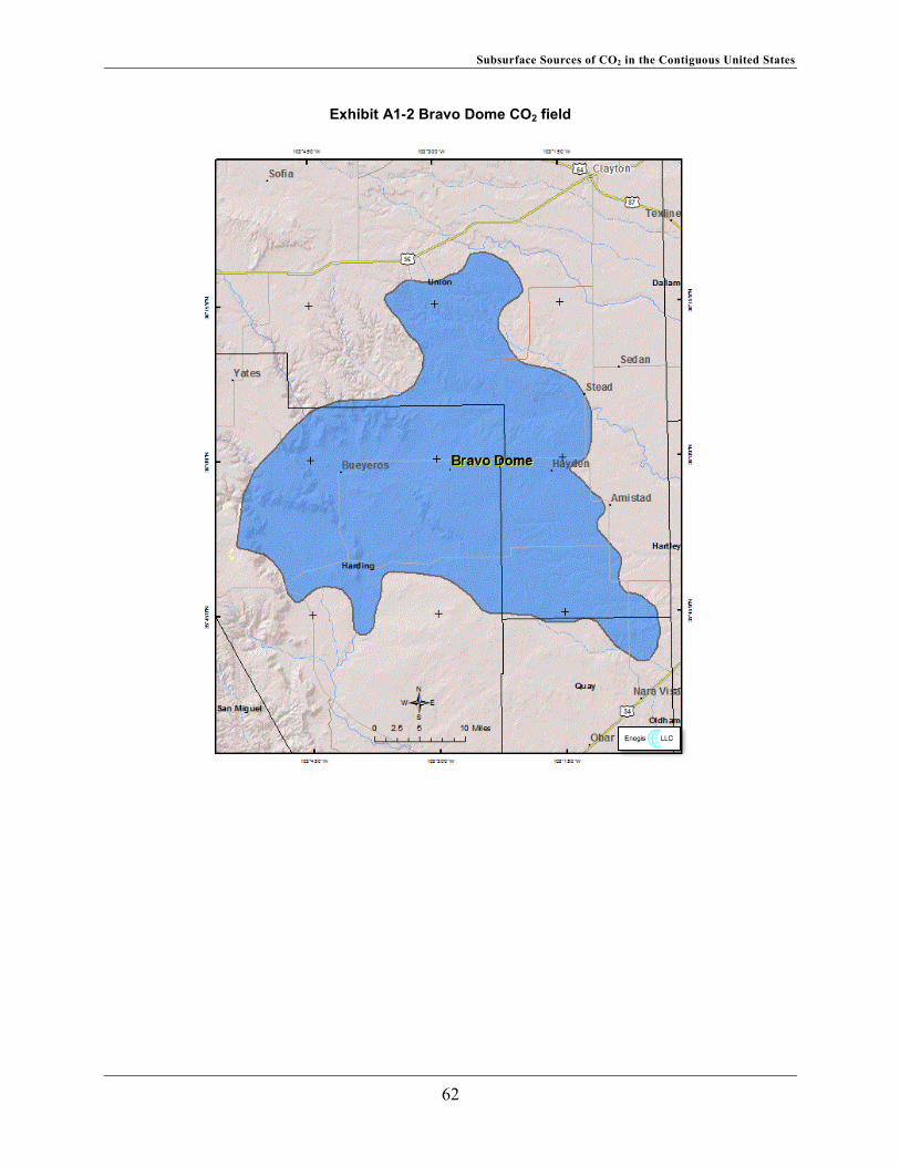
Subsurface Sources of CO2 in the Contiguous United States
Exhibit A1-2 Bravo Dome CO2 field
62
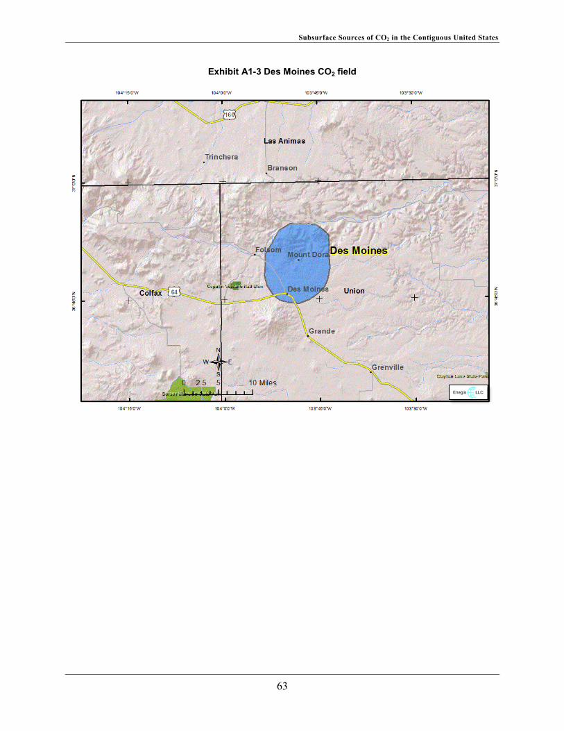
Subsurface Sources of CO2 in the Contiguous United States
Exhibit A1-3 Des Moines CO2 field
63
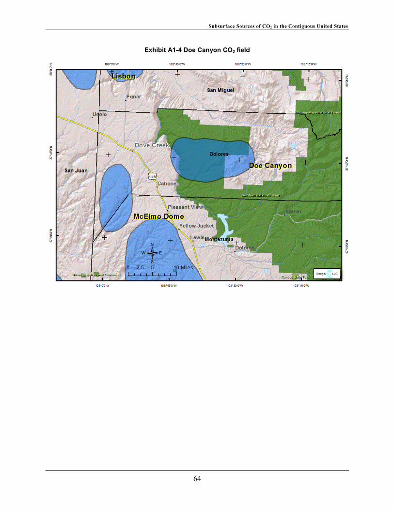
Subsurface Sources of CO2 in the Contiguous United States
Exhibit A1-4 Doe Canyon CO2 field
64
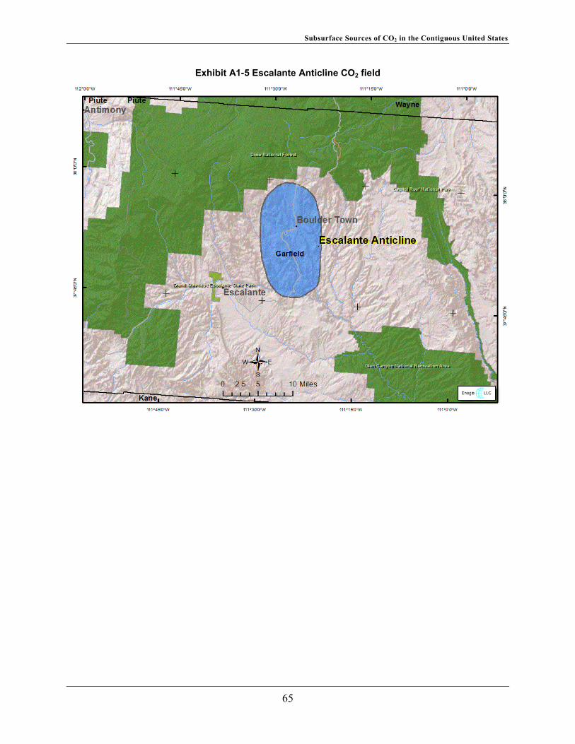
Subsurface Sources of CO2 in the Contiguous United States
Exhibit A1-5 Escalante Anticline CO2 field
65

Subsurface Sources of CO2 in the Contiguous United States
Exhibit A1-6 Estancia CO2 field
66
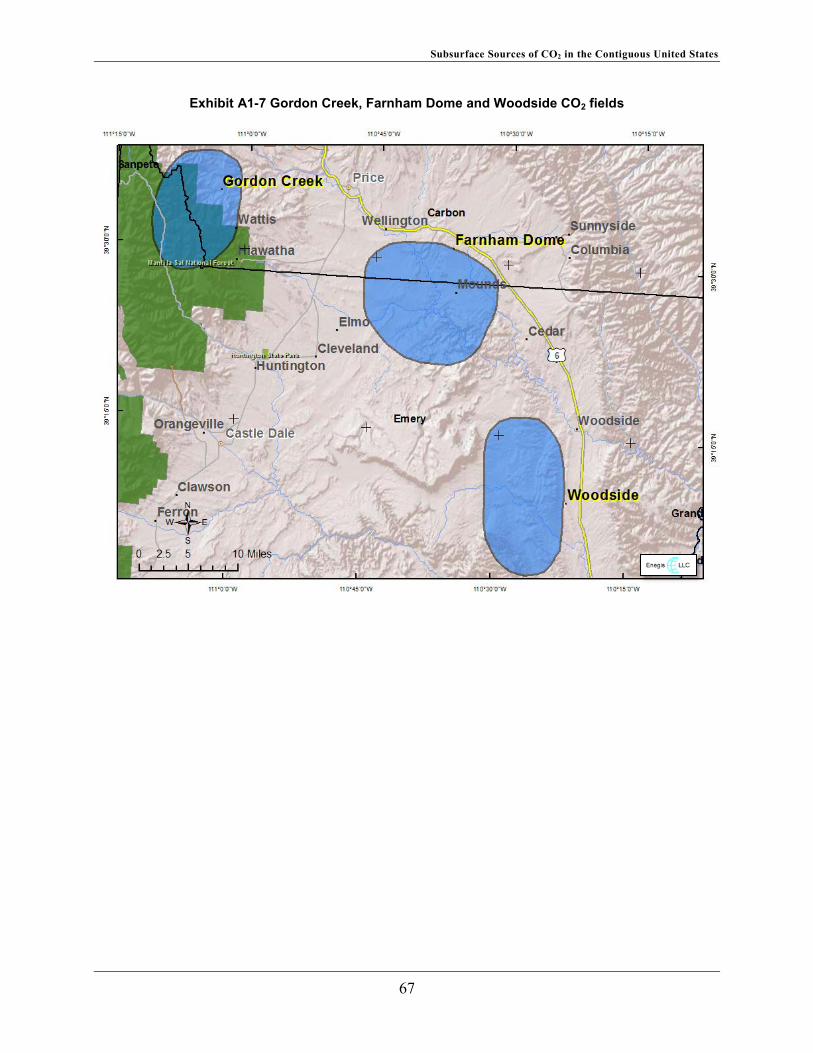
Subsurface Sources of CO2 in the Contiguous United States
Exhibit A1-7 Gordon Creek, Farnham Dome and Woodside CO2 fields
67

Subsurface Sources of CO2 in the Contiguous United States
Exhibit A1-8 Imperial CO2 field
68
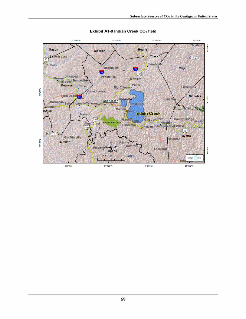
Subsurface Sources of CO2 in the Contiguous United States
Exhibit A1-9 Indian Creek CO2 field
69
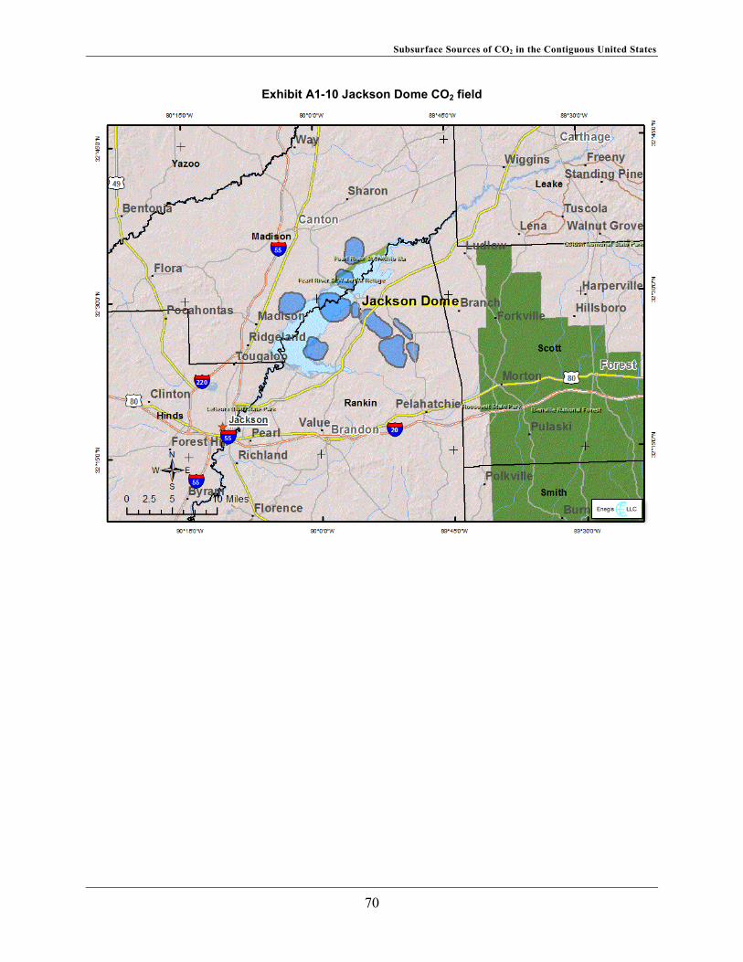
Subsurface Sources of CO2 in the Contiguous United States
Exhibit A1-10 Jackson Dome CO2 field
70

Subsurface Sources of CO2 in the Contiguous United States
Exhibit A1-11 Kevin Dome CO2 field
71
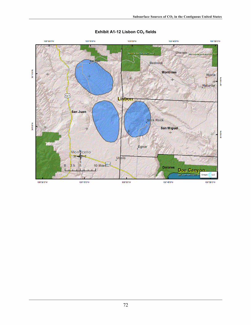
Subsurface Sources of CO2 in the Contiguous United States
Exhibit A1-12 Lisbon CO2 fields
72

Subsurface Sources of CO2 in the Contiguous United States
Exhibit A1-13 Madden CO2 field
73
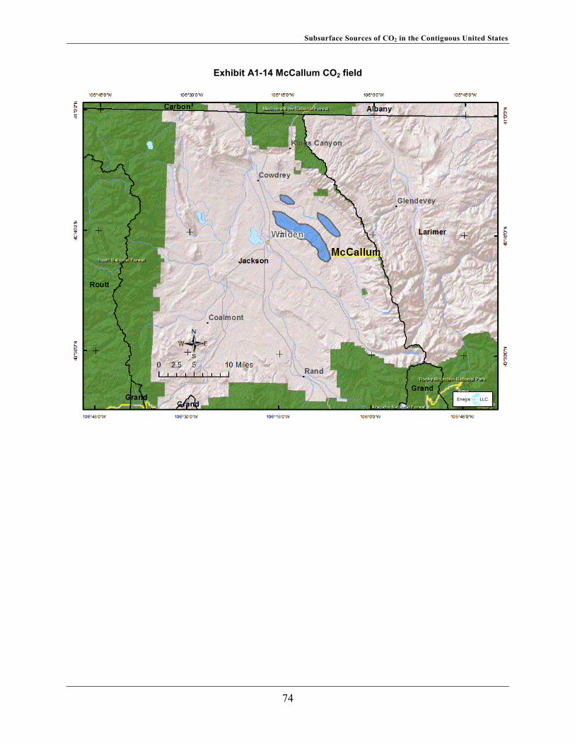
Subsurface Sources of CO2 in the Contiguous United States
Exhibit A1-14 McCallum CO2 field
74
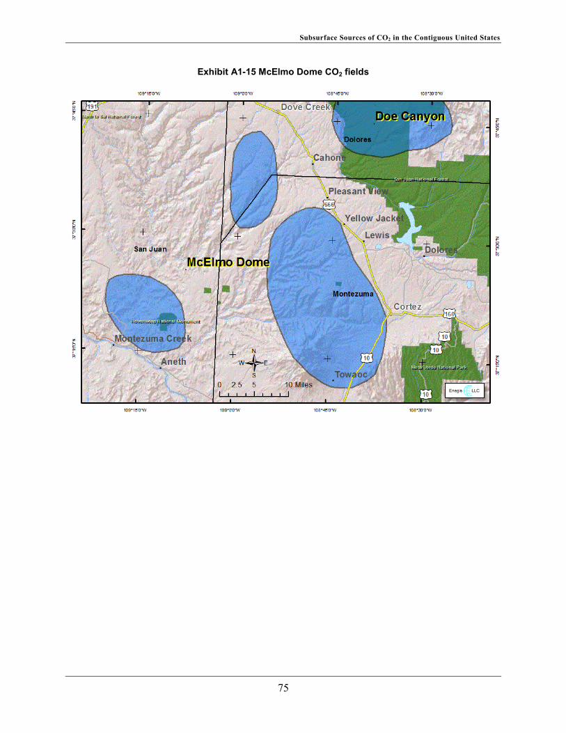
Subsurface Sources of CO2 in the Contiguous United States
Exhibit A1-15 McElmo Dome CO2 fields
75
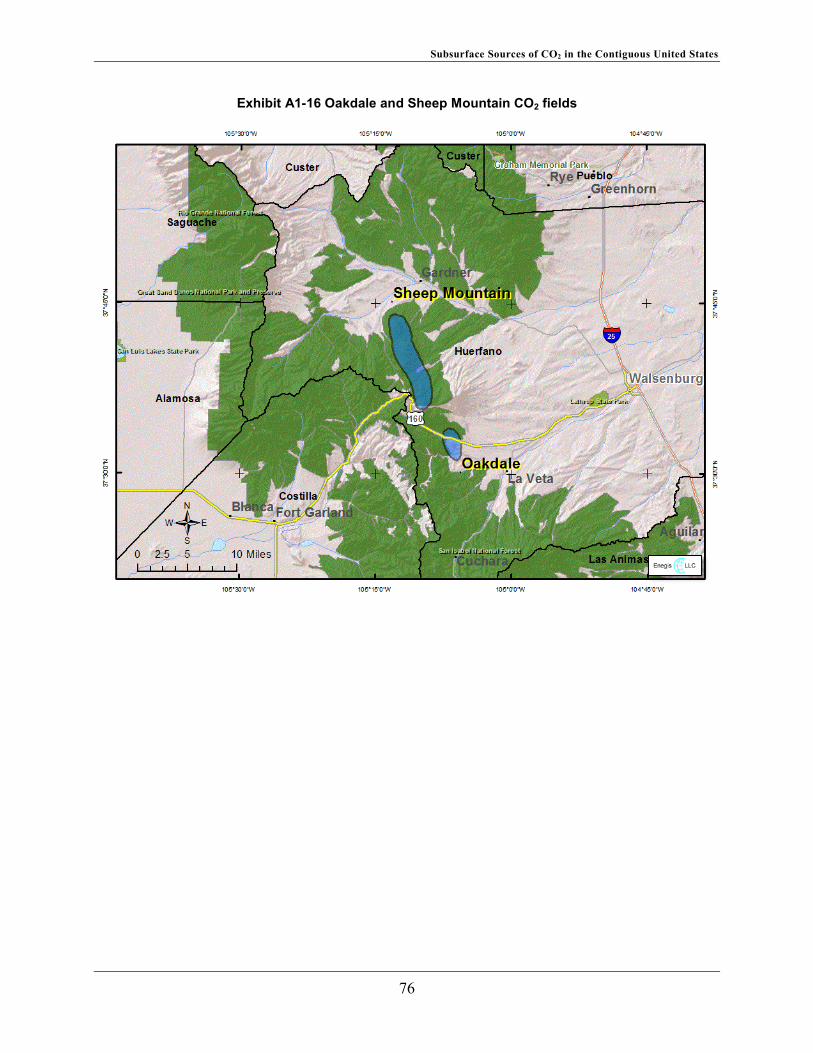
Subsurface Sources of CO2 in the Contiguous United States
Exhibit A1-16 Oakdale and Sheep Mountain CO2 fields
76

Subsurface Sources of CO2 in the Contiguous United States
Exhibit A1-17 St. Johns/Springerville CO2 field
77
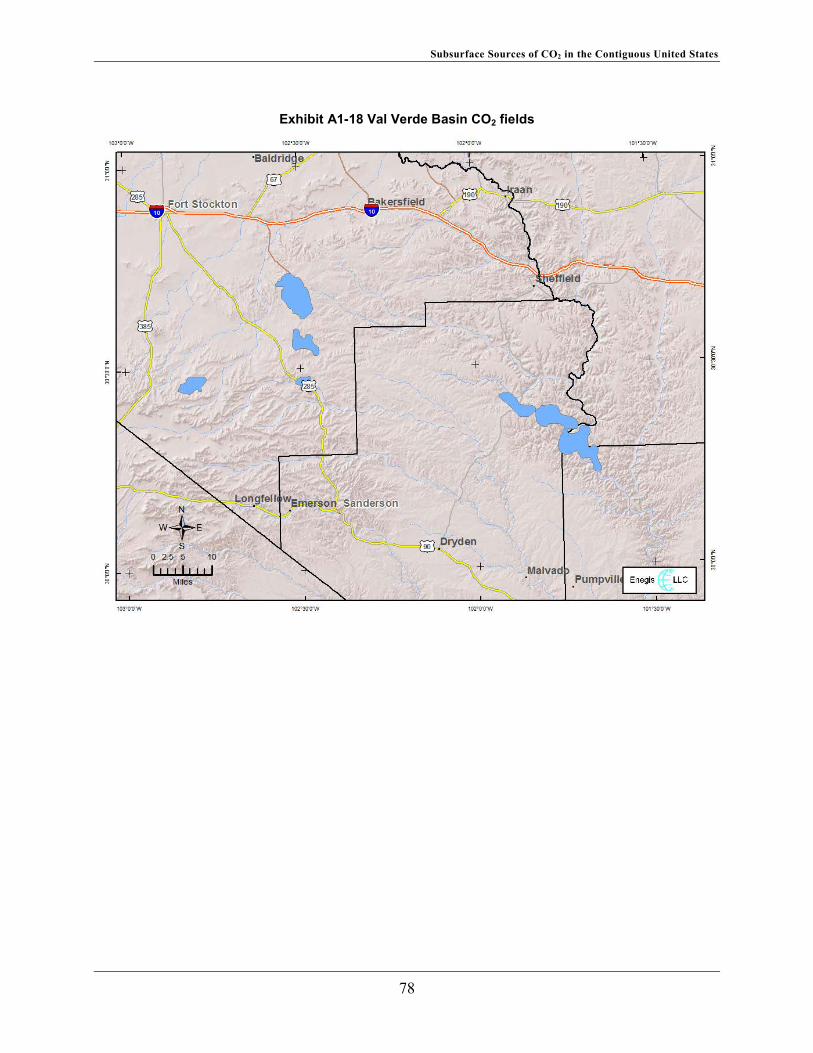
Subsurface Sources of CO2 in the Contiguous United States
Exhibit A1-18 Val Verde Basin CO2 fields
78

Subsurface Sources of CO2 in the Contiguous United States
This page intentionally left blank.
79
Subsurface Sources of CO2 in the Contiguous United States
Appendix 2 Disaggregated Field Parameters and Results from CREAM1
1 Also available in accompanying spreadsheet
80
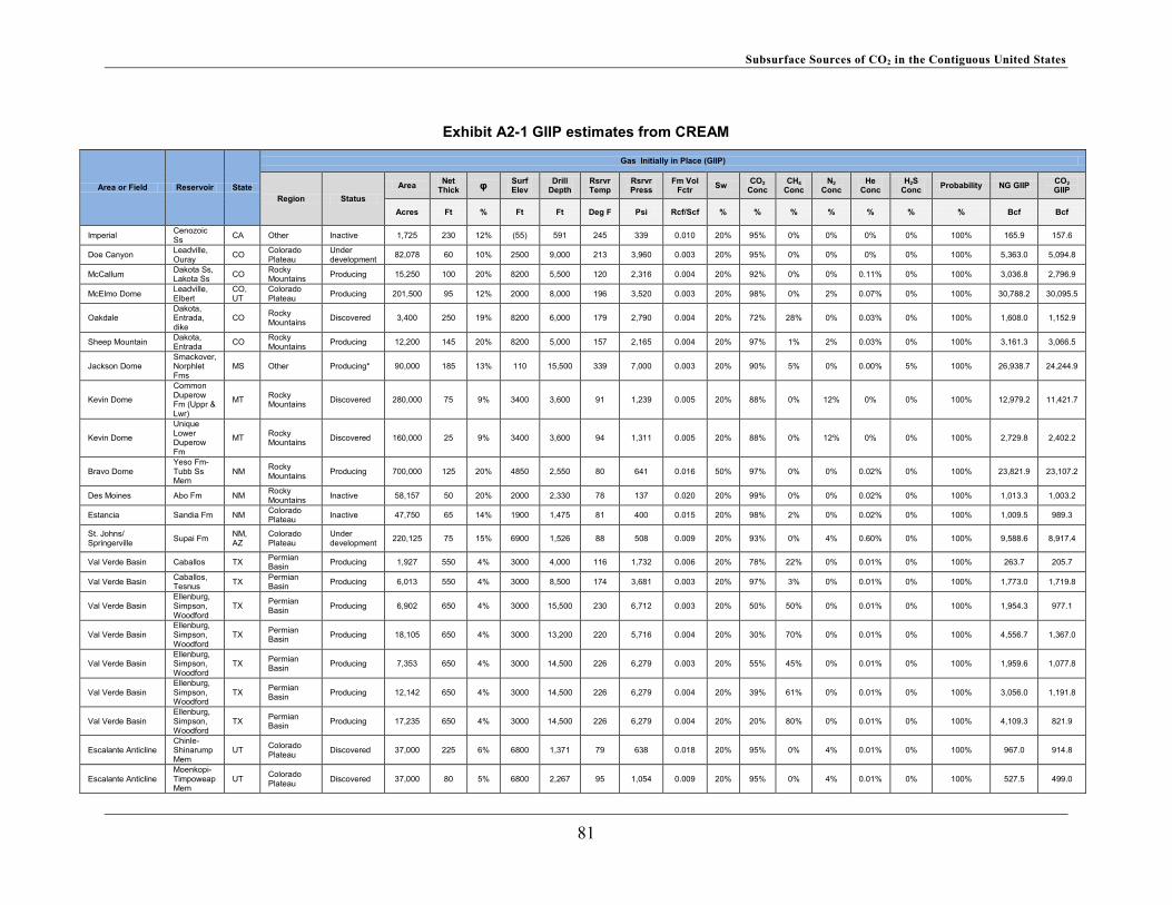
Subsurface Sources of CO2 in the Contiguous United States
Exhibit A2-1 GIIP estimates from CREAM
Area or Field Reservoir State
Gas Initially in Place (GIIP)
Region Status Area Net
Thick Surf Elev
Drill Depth
Rsrvr Temp
Rsrvr Press
Fm Vol Fctr Sw CO2
Conc CH4
Conc N2
Conc He
Conc H2S
Conc Probability NG GIIP CO2 GIIP
Acres Ft % Ft Ft Deg F Psi Rcf/Scf % % % % % % % Bcf Bcf
Imperial Cenozoic Ss CA Other Inactive 1,725 230 12% (55) 591 245 339 0.010 20% 95% 0% 0% 0% 0% 100% 165.9 157.6
Doe Canyon Leadville, Ouray CO Colorado
Plateau Under development 82,078 60 10% 2500 9,000 213 3,960 0.003 20% 95% 0% 0% 0% 0% 100% 5,363.0 5,094.8
McCallum Dakota Ss, Lakota Ss CO Rocky
Mountains Producing 15,250 100 20% 8200 5,500 120 2,316 0.004 20% 92% 0% 0% 0.11% 0% 100% 3,036.8 2,796.9
McElmo Dome Leadville, Elbert
CO, UT
Colorado Plateau Producing 201,500 95 12% 2000 8,000 196 3,520 0.003 20% 98% 0% 2% 0.07% 0% 100% 30,788.2 30,095.5
Oakdale Dakota, Entrada, dike
CO Rocky Mountains Discovered 3,400 250 19% 8200 6,000 179 2,790 0.004 20% 72% 28% 0% 0.03% 0% 100% 1,608.0 1,152.9
Sheep Mountain Dakota, Entrada CO Rocky
Mountains Producing 12,200 145 20% 8200 5,000 157 2,165 0.004 20% 97% 1% 2% 0.03% 0% 100% 3,161.3 3,066.5
Jackson Dome Smackover, Norphlet Fms
MS Other Producing* 90,000 185 13% 110 15,500 339 7,000 0.003 20% 90% 5% 0% 0.00% 5% 100% 26,938.7 24,244.9
Kevin Dome
Common Duperow Fm (Uppr & Lwr)
MT Rocky Mountains Discovered 280,000 75 9% 3400 3,600 91 1,239 0.005 20% 88% 0% 12% 0% 0% 100% 12,979.2 11,421.7
Kevin Dome
Unique Lower Duperow Fm
MT Rocky Mountains Discovered 160,000 25 9% 3400 3,600 94 1,311 0.005 20% 88% 0% 12% 0% 0% 100% 2,729.8 2,402.2
Bravo Dome Yeso Fm-Tubb Ss Mem
NM Rocky Mountains Producing 700,000 125 20% 4850 2,550 80 641 0.016 50% 97% 0% 0% 0.02% 0% 100% 23,821.9 23,107.2
Des Moines Abo Fm NM Rocky Mountains Inactive 58,157 50 20% 2000 2,330 78 137 0.020 20% 99% 0% 0% 0.02% 0% 100% 1,013.3 1,003.2
Estancia Sandia Fm NM Colorado Plateau Inactive 47,750 65 14% 1900 1,475 81 400 0.015 20% 98% 2% 0% 0.02% 0% 100% 1,009.5 989.3
St. Johns/ Springerville Supai Fm NM,
AZ Colorado Plateau
Under development 220,125 75 15% 6900 1,526 88 508 0.009 20% 93% 0% 4% 0.60% 0% 100% 9,588.6 8,917.4
Val Verde Basin Caballos TX Permian Basin Producing 1,927 550 4% 3000 4,000 116 1,732 0.006 20% 78% 22% 0% 0.01% 0% 100% 263.7 205.7
Val Verde Basin Caballos, Tesnus TX Permian
Basin Producing 6,013 550 4% 3000 8,500 174 3,681 0.003 20% 97% 3% 0% 0.01% 0% 100% 1,773.0 1,719.8
Val Verde Basin Ellenburg, Simpson, Woodford
TX Permian Basin Producing 6,902 650 4% 3000 15,500 230 6,712 0.003 20% 50% 50% 0% 0.01% 0% 100% 1,954.3 977.1
Val Verde Basin Ellenburg, Simpson, Woodford
TX Permian Basin Producing 18,105 650 4% 3000 13,200 220 5,716 0.004 20% 30% 70% 0% 0.01% 0% 100% 4,556.7 1,367.0
Val Verde Basin Ellenburg, Simpson, Woodford
TX Permian Basin Producing 7,353 650 4% 3000 14,500 226 6,279 0.003 20% 55% 45% 0% 0.01% 0% 100% 1,959.6 1,077.8
Val Verde Basin Ellenburg, Simpson, Woodford
TX Permian Basin Producing 12,142 650 4% 3000 14,500 226 6,279 0.004 20% 39% 61% 0% 0.01% 0% 100% 3,056.0 1,191.8
Val Verde Basin Ellenburg, Simpson, Woodford
TX Permian Basin Producing 17,235 650 4% 3000 14,500 226 6,279 0.004 20% 20% 80% 0% 0.01% 0% 100% 4,109.3 821.9
Escalante Anticline Chinle-Shinarump Mem
UT Colorado Plateau Discovered 37,000 225 6% 6800 1,371 79 638 0.018 20% 95% 0% 4% 0.01% 0% 100% 967.0 914.8
Escalante Anticline Moenkopi-Timpoweap Mem
UT Colorado Plateau Discovered 37,000 80 5% 6800 2,267 95 1,054 0.009 20% 95% 0% 4% 0.01% 0% 100% 527.5 499.0
81
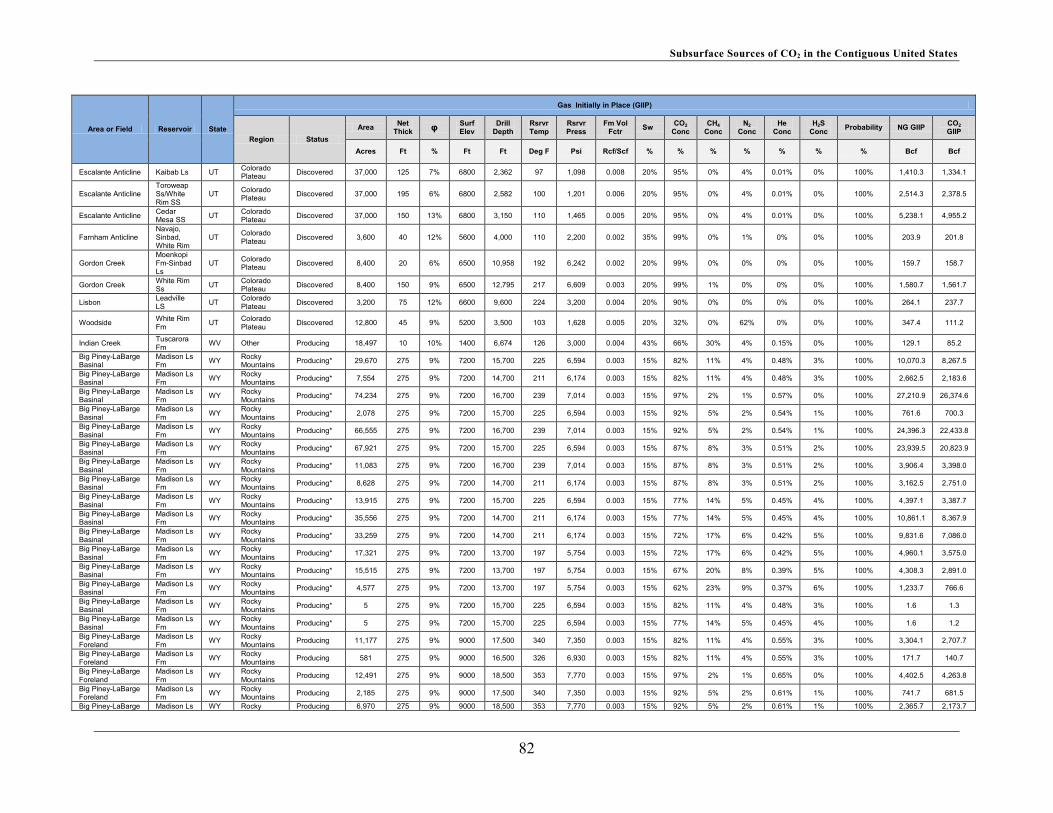
Subsurface Sources of CO2 in the Contiguous United States
Area or Field Reservoir State
Gas Initially in Place (GIIP)
Region Status Area Net
Thick Surf Elev
Drill Depth
Rsrvr Temp
Rsrvr Press
Fm Vol Fctr Sw CO2
Conc CH4
Conc N2
Conc He
Conc H2S
Conc Probability NG GIIP CO2 GIIP
Acres Ft % Ft Ft Deg F Psi Rcf/Scf % % % % % % % Bcf Bcf
Escalante Anticline Kaibab Ls UT Colorado Plateau Discovered 37,000 125 7% 6800 2,362 97 1,098 0.008 20% 95% 0% 4% 0.01% 0% 100% 1,410.3 1,334.1
Escalante Anticline Toroweap Ss/White Rim SS
UT Colorado Plateau Discovered 37,000 195 6% 6800 2,582 100 1,201 0.006 20% 95% 0% 4% 0.01% 0% 100% 2,514.3 2,378.5
Escalante Anticline Cedar Mesa SS UT Colorado
Plateau Discovered 37,000 150 13% 6800 3,150 110 1,465 0.005 20% 95% 0% 4% 0.01% 0% 100% 5,238.1 4,955.2
Farnham Anticline Navajo, Sinbad, White Rim
UT Colorado Plateau Discovered 3,600 40 12% 5600 4,000 110 2,200 0.002 35% 99% 0% 1% 0% 0% 100% 203.9 201.8
Gordon Creek Moenkopi Fm-Sinbad Ls
UT Colorado Plateau Discovered 8,400 20 6% 6500 10,958 192 6,242 0.002 20% 99% 0% 0% 0% 0% 100% 159.7 158.7
Gordon Creek White Rim Ss UT Colorado
Plateau Discovered 8,400 150 9% 6500 12,795 217 6,609 0.003 20% 99% 1% 0% 0% 0% 100% 1,580.7 1,561.7
Lisbon Leadville LS UT Colorado
Plateau Discovered 3,200 75 12% 6600 9,600 224 3,200 0.004 20% 90% 0% 0% 0% 0% 100% 264.1 237.7
Woodside White Rim Fm UT Colorado
Plateau Discovered 12,800 45 9% 5200 3,500 103 1,628 0.005 20% 32% 0% 62% 0% 0% 100% 347.4 111.2
Indian Creek Tuscarora Fm WV Other Producing 18,497 10 10% 1400 6,674 126 3,000 0.004 43% 66% 30% 4% 0.15% 0% 100% 129.1 85.2
Big Piney-LaBarge Basinal
Madison Ls Fm WY Rocky
Mountains Producing* 29,670 275 9% 7200 15,700 225 6,594 0.003 15% 82% 11% 4% 0.48% 3% 100% 10,070.3 8,267.5
Big Piney-LaBarge Basinal
Madison Ls Fm WY Rocky
Mountains Producing* 7,554 275 9% 7200 14,700 211 6,174 0.003 15% 82% 11% 4% 0.48% 3% 100% 2,662.5 2,183.6
Big Piney-LaBarge Basinal
Madison Ls Fm WY Rocky
Mountains Producing* 74,234 275 9% 7200 16,700 239 7,014 0.003 15% 97% 2% 1% 0.57% 0% 100% 27,210.9 26,374.6
Big Piney-LaBarge Basinal
Madison Ls Fm WY Rocky
Mountains Producing* 2,078 275 9% 7200 15,700 225 6,594 0.003 15% 92% 5% 2% 0.54% 1% 100% 761.6 700.3
Big Piney-LaBarge Basinal
Madison Ls Fm WY Rocky
Mountains Producing* 66,555 275 9% 7200 16,700 239 7,014 0.003 15% 92% 5% 2% 0.54% 1% 100% 24,396.3 22,433.8
Big Piney-LaBarge Basinal
Madison Ls Fm WY Rocky
Mountains Producing* 67,921 275 9% 7200 15,700 225 6,594 0.003 15% 87% 8% 3% 0.51% 2% 100% 23,939.5 20,823.9
Big Piney-LaBarge Basinal
Madison Ls Fm WY Rocky
Mountains Producing* 11,083 275 9% 7200 16,700 239 7,014 0.003 15% 87% 8% 3% 0.51% 2% 100% 3,906.4 3,398.0
Big Piney-LaBarge Basinal
Madison Ls Fm WY Rocky
Mountains Producing* 8,628 275 9% 7200 14,700 211 6,174 0.003 15% 87% 8% 3% 0.51% 2% 100% 3,162.5 2,751.0
Big Piney-LaBarge Basinal
Madison Ls Fm WY Rocky
Mountains Producing* 13,915 275 9% 7200 15,700 225 6,594 0.003 15% 77% 14% 5% 0.45% 4% 100% 4,397.1 3,387.7
Big Piney-LaBarge Basinal
Madison Ls Fm WY Rocky
Mountains Producing* 35,556 275 9% 7200 14,700 211 6,174 0.003 15% 77% 14% 5% 0.45% 4% 100% 10,861.1 8,367.9
Big Piney-LaBarge Basinal
Madison Ls Fm WY Rocky
Mountains Producing* 33,259 275 9% 7200 14,700 211 6,174 0.003 15% 72% 17% 6% 0.42% 5% 100% 9,831.6 7,086.0
Big Piney-LaBarge Basinal
Madison Ls Fm WY Rocky
Mountains Producing* 17,321 275 9% 7200 13,700 197 5,754 0.003 15% 72% 17% 6% 0.42% 5% 100% 4,960.1 3,575.0
Big Piney-LaBarge Basinal
Madison Ls Fm WY Rocky
Mountains Producing* 15,515 275 9% 7200 13,700 197 5,754 0.003 15% 67% 20% 8% 0.39% 5% 100% 4,308.3 2,891.0
Big Piney-LaBarge Basinal
Madison Ls Fm WY Rocky
Mountains Producing* 4,577 275 9% 7200 13,700 197 5,754 0.003 15% 62% 23% 9% 0.37% 6% 100% 1,233.7 766.6
Big Piney-LaBarge Basinal
Madison Ls Fm WY Rocky
Mountains Producing* 5 275 9% 7200 15,700 225 6,594 0.003 15% 82% 11% 4% 0.48% 3% 100% 1.6 1.3
Big Piney-LaBarge Basinal
Madison Ls Fm WY Rocky
Mountains Producing* 5 275 9% 7200 15,700 225 6,594 0.003 15% 77% 14% 5% 0.45% 4% 100% 1.6 1.2
Big Piney-LaBarge Foreland
Madison Ls Fm WY Rocky
Mountains Producing 11,177 275 9% 9000 17,500 340 7,350 0.003 15% 82% 11% 4% 0.55% 3% 100% 3,304.1 2,707.7
Big Piney-LaBarge Foreland
Madison Ls Fm WY Rocky
Mountains Producing 581 275 9% 9000 16,500 326 6,930 0.003 15% 82% 11% 4% 0.55% 3% 100% 171.7 140.7
Big Piney-LaBarge Foreland
Madison Ls Fm WY Rocky
Mountains Producing 12,491 275 9% 9000 18,500 353 7,770 0.003 15% 97% 2% 1% 0.65% 0% 100% 4,402.5 4,263.8
Big Piney-LaBarge Foreland
Madison Ls Fm WY Rocky
Mountains Producing 2,185 275 9% 9000 17,500 340 7,350 0.003 15% 92% 5% 2% 0.61% 1% 100% 741.7 681.5
Big Piney-LaBarge Madison Ls WY Rocky Producing 6,970 275 9% 9000 18,500 353 7,770 0.003 15% 92% 5% 2% 0.61% 1% 100% 2,365.7 2,173.7
82
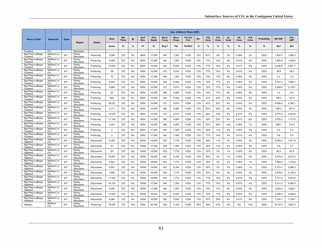
Subsurface Sources of CO2 in the Contiguous United States
Area or Field Reservoir State
Gas Initially in Place (GIIP)
Region Status Area Net
Thick Surf Elev
Drill Depth
Rsrvr Temp
Rsrvr Press
Fm Vol Fctr Sw CO2
Conc CH4
Conc N2
Conc He
Conc H2S
Conc Probability NG GIIP CO2 GIIP
Acres Ft % Ft Ft Deg F Psi Rcf/Scf % % % % % % % Bcf Bcf
Foreland Fm Mountains Big Piney-LaBarge Foreland
Madison Ls Fm WY Rocky
Mountains Producing 5,598 275 9% 9000 17,500 340 7,350 0.003 15% 87% 8% 3% 0.58% 2% 100% 1,832.0 1,592.3
Big Piney-LaBarge Foreland
Madison Ls Fm WY Rocky
Mountains Producing 6,308 275 9% 9000 17,500 340 7,350 0.003 15% 77% 14% 5% 0.51% 4% 100% 1,864.8 1,435.6
Big Piney-LaBarge Foreland
Madison Ls Fm WY Rocky
Mountains Producing 13,870 275 9% 9000 16,500 326 6,930 0.003 15% 77% 14% 5% 0.51% 4% 100% 4,236.9 3,261.7
Big Piney-LaBarge Foreland
Madison Ls Fm WY Rocky
Mountains Producing 125 275 9% 9000 15,500 312 6,510 0.003 15% 77% 14% 5% 0.51% 4% 100% 36.8 28.3
Big Piney-LaBarge Foreland
Madison Ls Fm WY Rocky
Mountains Producing 15 275 9% 9000 17,500 340 7,350 0.003 15% 72% 17% 6% 0.48% 5% 100% 4.2 3.0
Big Piney-LaBarge Foreland
Madison Ls Fm WY Rocky
Mountains Producing 9,524 275 9% 9000 16,500 326 6,930 0.003 15% 72% 17% 6% 0.48% 5% 100% 2,727.3 1,964.1
Big Piney-LaBarge Foreland
Madison Ls Fm WY Rocky
Mountains Producing 9,999 275 9% 9000 15,500 312 6,510 0.003 15% 72% 17% 6% 0.48% 5% 100% 2,955.8 2,128.7
Big Piney-LaBarge Foreland
Madison Ls Fm WY Rocky
Mountains Producing 23 275 9% 9000 14,500 298 6,090 0.003 15% 72% 17% 6% 0.48% 5% 100% 7.0 5.0
Big Piney-LaBarge Foreland
Madison Ls Fm WY Rocky
Mountains Producing 682 275 9% 9000 16,500 326 6,930 0.003 15% 67% 20% 8% 0.45% 5% 100% 189.4 127.0
Big Piney-LaBarge Foreland
Madison Ls Fm WY Rocky
Mountains Producing 26,231 275 9% 9000 15,500 312 6,510 0.004 15% 67% 20% 8% 0.45% 5% 100% 6,496.8 4,356.1
Big Piney-LaBarge Foreland
Madison Ls Fm WY Rocky
Mountains Producing 2,171 275 9% 9000 14,500 298 6,090 0.004 15% 67% 20% 8% 0.45% 5% 100% 568.3 381.0
Big Piney-LaBarge Foreland
Madison Ls Fm WY Rocky
Mountains Producing 16,479 275 9% 9000 15,500 312 6,510 0.004 15% 62% 23% 9% 0.41% 6% 100% 3,775.3 2,343.8
Big Piney-LaBarge Foreland
Madison Ls Fm WY Rocky
Mountains Producing 11,140 275 9% 9000 14,500 298 6,090 0.004 15% 62% 23% 9% 0.41% 6% 100% 2,759.2 1,713.0
Big Piney-LaBarge Foreland
Madison Ls Fm WY Rocky
Mountains Producing 2,257 275 9% 9000 14,500 298 6,090 0.004 15% 57% 26% 10% 0.38% 7% 100% 559.1 319.3
Big Piney-LaBarge Foreland
Madison Ls Fm WY Rocky
Mountains Producing 2 275 9% 9000 17,500 340 7,350 0.003 15% 82% 11% 4% 0.55% 3% 100% 0.6 0.5
Big Piney-LaBarge Foreland
Madison Ls Fm WY Rocky
Mountains Producing 2 275 9% 9000 17,500 340 7,350 0.003 15% 77% 14% 5% 0.51% 4% 100% 0.6 0.5
Big Piney-LaBarge Highland
Madison Ls Fm WY Rocky
Mountains Discovered 31,651 275 9% 10000 18,500 353 7,770 0.003 15% 82% 11% 4% 0.50% 3% 100% 9,356.3 7,671.9
Big Piney-LaBarge Highland
Madison Ls Fm WY Rocky
Mountains Discovered 23 275 9% 10000 17,500 340 7,350 0.003 15% 82% 11% 4% 0.50% 3% 100% 6.9 5.7
Big Piney-LaBarge Highland
Madison Ls Fm WY Rocky
Mountains Discovered 221 275 9% 10000 18,500 353 7,770 0.002 15% 97% 2% 1% 0.59% 0% 100% 84.5 81.9
Big Piney-LaBarge Highland
Madison Ls Fm WY Rocky
Mountains Discovered 14,951 275 9% 10000 19,500 367 8,190 0.003 15% 97% 2% 1% 0.59% 0% 100% 5,074.4 4,917.4
Big Piney-LaBarge Highland
Madison Ls Fm WY Rocky
Mountains Discovered 5,553 275 9% 10000 18,500 353 7,770 0.003 15% 92% 5% 2% 0.56% 1% 100% 1,884.6 1,732.6
Big Piney-LaBarge Highland
Madison Ls Fm WY Rocky
Mountains Discovered 6,947 275 9% 10000 19,500 367 8,190 0.003 15% 92% 5% 2% 0.56% 1% 100% 2,273.7 2,090.3
Big Piney-LaBarge Highland
Madison Ls Fm WY Rocky
Mountains Discovered 7,696 275 9% 10000 18,500 353 7,770 0.003 15% 87% 8% 3% 0.53% 2% 100% 2,518.9 2,190.6
Big Piney-LaBarge Highland
Madison Ls Fm WY Rocky
Mountains Discovered 11,443 275 9% 10000 18,500 353 7,770 0.003 15% 77% 14% 5% 0.47% 4% 100% 3,177.8 2,447.8
Big Piney-LaBarge Highland
Madison Ls Fm WY Rocky
Mountains Discovered 19,125 275 9% 10000 17,500 340 7,350 0.003 15% 77% 14% 5% 0.47% 4% 100% 5,311.0 4,090.9
Big Piney-LaBarge Highland
Madison Ls Fm WY Rocky
Mountains Discovered 8,006 275 9% 10000 17,500 340 7,350 0.003 15% 72% 17% 6% 0.44% 5% 100% 2,223.3 1,602.1
Big Piney-LaBarge Highland
Madison Ls Fm WY Rocky
Mountains Discovered 12,342 275 9% 10000 16,500 326 6,930 0.003 15% 72% 17% 6% 0.44% 5% 100% 3,326.4 2,396.9
Big Piney-LaBarge Highland
Madison Ls Fm WY Rocky
Mountains Discovered 6,585 275 9% 10000 16,500 326 6,930 0.004 15% 67% 20% 8% 0.41% 5% 100% 1,724.1 1,156.7
Madden Madison Fm WY Rocky
Mountains Producing* 79,500 175 15% 5350 23,700 335 11,021 0.004 20% 20% 67% 0% 0% 12% 100% 19,137.7 3,827.5
83

Subsurface Sources of CO2 in the Contiguous United States
Exhibit A2-2 Accessible TRR estimates from CREAM
Area or Field
Accessible Technically Recoverable Resources (TRR)
Recovery Factor NG TRR Accessible
portion Accessible
NG TRR Accessible CO2 TRR No.
wells
NG TRR /well
NG EUR Tier, Average EUR Per Well
10% 20% 30% 40%
% Bcf % Bcf Bcf Bcf Bcf Bcf Bcf Bcf Imperial 65% 107.8 80% 86.3 82.0 25 3.45 5.6 5.3 3.6 1.9 Doe Canyon 70% 3,754.1 75% 2,815.6 2,674.8 96 29.3 47.6 44.7 30.5 16.2 McCallum 70% 2,125.7 90% 1,913.2 1,762.0 21 91.1 148.0 138.8 94.7 50.3 McElmo Dome 70% 21,551.7 65% 14,008.6 13,693.4 205 68.3 111.0 104.1 71.1 37.7 Oakdale 65% 1,045.2 80% 836.2 599.5 4 209.0 339.5 318.6 217.4 115.4 Sheep Mountain 65% 2,054.9 80% 1,643.9 1,594.6 15 109.6 178.0 167.0 114.0 60.5 Jackson Dome 70% 18,857.1 95% 17,914.3 16,122.8 134 133.7 217.1 203.7 139.0 73.8 Kevin Dome 75% 9,734.4 95% 9,247.7 8,138.0 416 22.2 36.1 33.9 23.1 12.3 Kevin Dome 75% 2,047.3 95% 1,945.0 1,711.6 238 8.2 13.3 12.5 8.5 4.5 Bravo Dome 65% 15,484.2 90% 13,935.8 13,517.7 984 14.2 23.0 21.6 14.7 7.8 Des Moines 65% 658.7 90% 592.8 586.9 82 7.2 11.7 11.0 7.5 4.0 Estancia 60% 605.7 95% 575.4 563.9 71 8.1 13.2 12.4 8.4 4.5 St. Johns/Springerville 70% 6,712.1 80% 5,369.6 4,993.8 275 19.5 41.0 25.1 20.3 10.8 Val Verde Basin 70% 184.6 95% 175.4 136.8 3 58.5 95.0 89.1 60.8 32.3 Val Verde Basin 70% 1,241.1 95% 1,179.1 1,143.7 9 131.0 212.8 199.7 136.2 72.3 Val Verde Basin 70% 1,368.0 95% 1,299.6 649.8 10 130.0 211.1 198.1 135.1 71.7 Val Verde Basin 70% 3,189.7 95% 3,030.2 909.1 27 112.2 182.3 171.0 116.7 61.9 Val Verde Basin 70% 1,371.7 95% 1,303.1 716.7 11 118.5 192.4 180.5 123.2 65.4 Val Verde Basin 70% 2,139.2 95% 2,032.2 792.6 18 112.9 183.4 172.1 117.4 62.3 Val Verde Basin 70% 2,876.5 95% 2,732.7 546.5 26 105.1 170.7 160.2 109.3 58.0 Escalante Anticline 55% 531.9 45% 239.3 226.4 26 9.2 15.0 14.0 9.6 5.1 Escalante Anticline 55% 290.1 45% 130.5 123.5 26 5.0 8.2 7.7 5.2 2.8 Escalante Anticline 55% 775.6 45% 349.0 330.2 26 13.4 21.8 20.5 14.0 7.4 Escalante Anticline 55% 1,382.9 45% 622.3 588.7 26 23.9 38.9 36.5 24.9 13.2 Escalante Anticline 55% 2,880.9 45% 1,296.4 1,226.4 26 49.9 81.0 76.0 51.9 27.5 Farnham Anticline 70% 142.7 45% 64.2 63.6 3 21.4 34.8 32.6 22.3 11.8 Gordon Creek 65% 103.8 90% 93.4 92.8 12 7.8 12.6 11.9 8.1 4.3 Gordon Creek 65% 1,027.5 90% 924.7 913.6 12 77.1 125.2 117.4 80.1 42.5 Lisbon 70% 184.9 85% 157.1 141.4 4 39.3 63.8 59.9 40.9 21.7 Woodside 60% 208.4 90% 187.6 60.0 18 10.4 16.9 15.9 10.8 5.8 Indian Creek 70% 90.4 95% 85.8 56.7 27 3.2 5.2 4.8 3.3 1.8 Big Piney-LaBarge Basinal 70% 7,049.2 85% 5,991.8 4,919.2 39 153.6 249.5 234.2 159.8 84.8 Big Piney-LaBarge Basinal 70% 1,863.7 85% 1,584.2 1,299.3 10 158.4 257.3 241.4 164.7 87.4 Big Piney-LaBarge Basinal 70% 19,047.6 85% 16,190.5 15,692.9 99 163.5 265.6 249.2 170.1 90.3 Big Piney-LaBarge Basinal 70% 533.1 85% 453.1 416.7 3 151.0 245.3 230.2 157.1 83.4 Big Piney-LaBarge Basinal 70% 17,077.4 85% 14,515.8 13,348.1 88 165.0 267.9 251.4 171.5 91.0 Big Piney-LaBarge Basinal 70% 16,757.7 85% 14,244.0 12,390.2 90 158.3 257.1 241.2 164.6 87.4 Big Piney-LaBarge Basinal 70% 2,734.5 85% 2,324.3 2,021.8 15 155.0 251.7 236.2 161.1 85.5 Big Piney-LaBarge Basinal 70% 2,213.8 85% 1,881.7 1,636.8 11 171.1 277.9 260.7 177.9 94.4 Big Piney-LaBarge Basinal 70% 3,077.9 85% 2,616.2 2,015.7 18 145.3 236.1 221.5 151.2 80.2 Big Piney-LaBarge Basinal 70% 7,602.8 85% 6,462.4 4,978.9 47 137.5 223.3 209.6 143.0 75.9 Big Piney-LaBarge Basinal 70% 6,882.1 85% 5,849.8 4,216.2 44 133.0 215.9 202.6 138.3 73.4 Big Piney-LaBarge Basinal 70% 3,472.1 85% 2,951.3 2,127.1 23 128.3 208.4 195.6 133.4 70.8 Big Piney-LaBarge Basinal 70% 3,015.8 85% 2,563.5 1,720.2 21 122.1 198.3 186.0 126.9 67.4 Big Piney-LaBarge Basinal 70% 863.6 85% 734.1 456.1 6 122.3 198.7 186.5 127.2 67.5 Big Piney-LaBarge Basinal 70% 1.1 85% 1.0 0.8 - - - - - - Big Piney-LaBarge Basinal 70% 1.1 85% 0.9 0.7 - - - - - - Big Piney-LaBarge Foreland 70% 2,312.9 80% 1,850.3 1,516.3 14 132.2 214.7 201.4 137.4 72.9 Big Piney-LaBarge Foreland 70% 120.2 80% 96.2 78.8 1 96.2 156.2 146.6 100.0 53.1 Big Piney-LaBarge Foreland 70% 3,081.7 80% 2,465.4 2,387.7 16 154.1 250.3 234.8 160.2 85.1 Big Piney-LaBarge Foreland 70% 519.2 80% 415.3 381.6 3 138.4 224.9 211.0 144.0 76.4 Big Piney-LaBarge Foreland 70% 1,656.0 80% 1,324.8 1,217.3 9 147.2 239.1 224.3 153.1 81.2 Big Piney-LaBarge Foreland 70% 1,282.4 80% 1,025.9 891.7 7 146.6 238.1 223.4 152.4 80.9 Big Piney-LaBarge Foreland 70% 1,305.4 80% 1,044.3 803.9 8 130.5 212.0 198.9 135.7 72.1 Big Piney-LaBarge Foreland 70% 2,965.8 80% 2,372.6 1,826.5 17 139.6 226.7 212.7 145.1 77.0 Big Piney-LaBarge Foreland 70% 25.8 80% 20.6 15.9 - - - - - - Big Piney-LaBarge Foreland 70% 2.9 80% 2.3 1.7 - - - - - - Big Piney-LaBarge Foreland 70% 1,909.1 80% 1,527.3 1,099.9 12 127.3 206.7 194.0 132.4 70.3 Big Piney-LaBarge Foreland 70% 2,069.1 80% 1,655.3 1,192.1 12 137.9 224.0 210.2 143.4 76.1 Big Piney-LaBarge Foreland 70% 4.9 80% 3.9 2.8 - - - - - - Big Piney-LaBarge Foreland 70% 132.5 80% 106.0 71.1 1 106.0 172.2 161.6 110.3 58.5 Big Piney-LaBarge Foreland 70% 4,547.7 80% 3,638.2 2,439.4 33 110.2 179.1 168.0 114.7 60.9 Big Piney-LaBarge Foreland 70% 397.8 80% 318.2 213.4 3 106.1 172.3 161.7 110.3 58.6 Big Piney-LaBarge Foreland 70% 2,642.7 80% 2,114.2 1,312.5 21 100.7 163.5 153.4 104.7 55.6 Big Piney-LaBarge Foreland 70% 1,931.4 80% 1,545.2 959.3 14 110.4 179.3 168.2 114.8 60.9
84
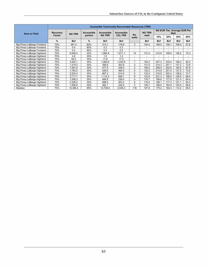
Subsurface Sources of CO2 in the Contiguous United States
Area or Field
Accessible Technically Recoverable Resources (TRR)
Recovery Factor NG TRR Accessible
portion Accessible
NG TRR Accessible CO2 TRR No.
wells
NG TRR /well
NG EUR Tier, Average EUR Per Well
10% 20% 30% 40%
% Bcf % Bcf Bcf Bcf Bcf Bcf Bcf Bcf Big Piney-LaBarge Foreland 70% 391.4 80% 313.1 178.8 3 104.4 169.5 159.1 108.5 57.6 Big Piney-LaBarge Foreland 70% 0.4 80% 0.3 0.3 - - - - - - Big Piney-LaBarge Foreland 70% 0.4 80% 0.3 0.3 - - - - - - Big Piney-LaBarge Highland 70% 6,549.4 30% 1,964.8 1,611.1 15 131.0 212.8 199.6 136.2 72.3 Big Piney-LaBarge Highland 70% 4.8 30% 1.5 1.2 - - - - - - Big Piney-LaBarge Highland 70% 59.2 30% 17.8 17.2 - - - - - - Big Piney-LaBarge Highland 70% 3,552.1 30% 1,065.6 1,032.6 7 152.2 247.3 232.0 158.3 84.0 Big Piney-LaBarge Highland 70% 1,319.2 30% 395.8 363.8 3 131.9 214.3 201.1 137.2 72.8 Big Piney-LaBarge Highland 70% 1,591.6 30% 477.5 439.0 3 159.2 258.5 242.6 165.5 87.8 Big Piney-LaBarge Highland 70% 1,763.2 30% 529.0 460.0 4 132.2 214.8 201.5 137.5 73.0 Big Piney-LaBarge Highland 70% 2,224.4 30% 667.3 514.0 5 133.5 216.8 203.4 138.8 73.7 Big Piney-LaBarge Highland 70% 3,717.7 30% 1,115.3 859.1 9 123.9 201.3 188.9 128.9 68.4 Big Piney-LaBarge Highland 70% 1,556.3 30% 466.9 336.4 4 116.7 189.6 177.9 121.4 64.4 Big Piney-LaBarge Highland 70% 2,328.5 30% 698.5 503.4 6 116.4 189.1 177.4 121.1 64.3 Big Piney-LaBarge Highland 70% 1,206.9 30% 362.1 242.9 3 120.7 196.0 183.9 125.5 66.6 Madden 70% 13,396.4 95% 12,726.6 2,545.3 118 107.9 175.2 164.4 112.2 59.5
85
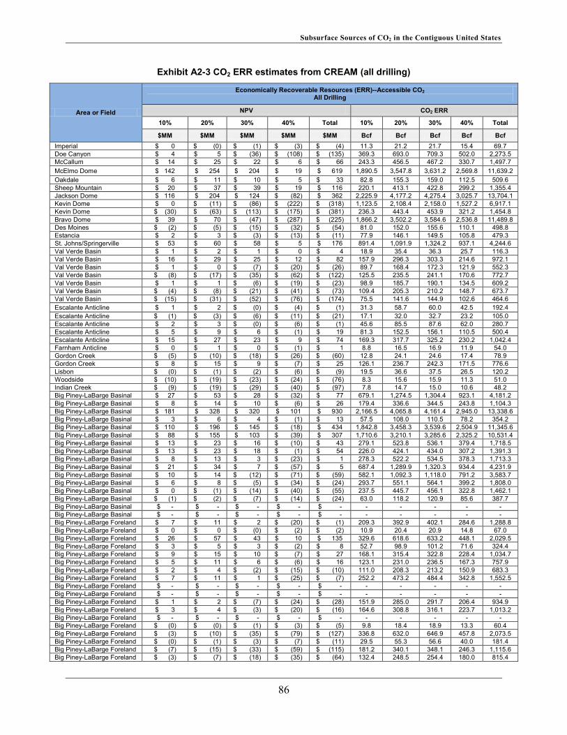
Subsurface Sources of CO2 in the Contiguous United States
Exhibit A2-3 CO2 ERR estimates from CREAM (all drilling)
Area or Field
Economically Recoverable Resources (ERR)--Accessible CO2 All Drilling
NPV CO2 ERR
10% 20% 30% 40% Total 10% 20% 30% 40% Total
$MM $MM $MM $MM $MM Bcf Bcf Bcf Bcf Bcf Imperial $ 0 $ (0) $ (1) $ (3) $ (4) 11.3 21.2 21.7 15.4 69.7 Doe Canyon $ 4 $ 5 $ (36) $ (108) $ (135) 369.3 693.0 709.3 502.0 2,273.5 McCallum $ 14 $ 25 $ 22 $ 6 $ 66 243.3 456.5 467.2 330.7 1,497.7 McElmo Dome $ 142 $ 254 $ 204 $ 19 $ 619 1,890.5 3,547.8 3,631.2 2,569.8 11,639.2 Oakdale $ 6 $ 11 $ 10 $ 5 $ 33 82.8 155.3 159.0 112.5 509.6 Sheep Mountain $ 20 $ 37 $ 39 $ 19 $ 116 220.1 413.1 422.8 299.2 1,355.4 Jackson Dome $ 116 $ 204 $ 124 $ (82) $ 362 2,225.9 4,177.2 4,275.4 3,025.7 13,704.1 Kevin Dome $ 0 $ (11) $ (86) $ (222) $ (318) 1,123.5 2,108.4 2,158.0 1,527.2 6,917.1 Kevin Dome $ (30) $ (63) $ (113) $ (175) $ (381) 236.3 443.4 453.9 321.2 1,454.8 Bravo Dome $ 39 $ 70 $ (47) $ (287) $ (225) 1,866.2 3,502.2 3,584.6 2,536.8 11,489.8 Des Moines $ (2) $ (5) $ (15) $ (32) $ (54) 81.0 152.0 155.6 110.1 498.8 Estancia $ 2 $ 3 $ (3) $ (13) $ (11) 77.9 146.1 149.5 105.8 479.3 St. Johns/Springerville $ 53 $ 60 $ 58 $ 5 $ 176 891.4 1,091.9 1,324.2 937.1 4,244.6 Val Verde Basin $ 1 $ 2 $ 1 $ 0 $ 4 18.9 35.4 36.3 25.7 116.3 Val Verde Basin $ 16 $ 29 $ 25 $ 12 $ 82 157.9 296.3 303.3 214.6 972.1 Val Verde Basin $ 1 $ 0 $ (7) $ (20) $ (26) 89.7 168.4 172.3 121.9 552.3 Val Verde Basin $ (8) $ (17) $ (35) $ (62) $ (122) 125.5 235.5 241.1 170.6 772.7 Val Verde Basin $ 1 $ 1 $ (6) $ (19) $ (23) 98.9 185.7 190.1 134.5 609.2 Val Verde Basin $ (4) $ (8) $ (21) $ (41) $ (73) 109.4 205.3 210.2 148.7 673.7 Val Verde Basin $ (15) $ (31) $ (52) $ (76) $ (174) 75.5 141.6 144.9 102.6 464.6 Escalante Anticline $ 1 $ 2 $ (0) $ (4) $ (1) 31.3 58.7 60.0 42.5 192.4 Escalante Anticline $ (1) $ (3) $ (6) $ (11) $ (21) 17.1 32.0 32.7 23.2 105.0 Escalante Anticline $ 2 $ 3 $ (0) $ (6) $ (1) 45.6 85.5 87.6 62.0 280.7 Escalante Anticline $ 5 $ 9 $ 6 $ (1) $ 19 81.3 152.5 156.1 110.5 500.4 Escalante Anticline $ 15 $ 27 $ 23 $ 9 $ 74 169.3 317.7 325.2 230.2 1,042.4 Farnham Anticline $ 0 $ 1 $ 0 $ (1) $ 1 8.8 16.5 16.9 11.9 54.0 Gordon Creek $ (5) $ (10) $ (18) $ (26) $ (60) 12.8 24.1 24.6 17.4 78.9 Gordon Creek $ 8 $ 15 $ 9 $ (7) $ 25 126.1 236.7 242.3 171.5 776.6 Lisbon $ (0) $ (1) $ (2) $ (6) $ (9) 19.5 36.6 37.5 26.5 120.2 Woodside $ (10) $ (19) $ (23) $ (24) $ (76) 8.3 15.6 15.9 11.3 51.0 Indian Creek $ (9) $ (19) $ (29) $ (40) $ (97) 7.8 14.7 15.0 10.6 48.2 Big Piney-LaBarge Basinal $ 27 $ 53 $ 28 $ (32) $ 77 679.1 1,274.5 1,304.4 923.1 4,181.2 Big Piney-LaBarge Basinal $ 8 $ 14 $ 10 $ (6) $ 26 179.4 336.6 344.5 243.8 1,104.3 Big Piney-LaBarge Basinal $ 181 $ 328 $ 320 $ 101 $ 930 2,166.5 4,065.8 4,161.4 2,945.0 13,338.6 Big Piney-LaBarge Basinal $ 3 $ 6 $ 4 $ (1) $ 13 57.5 108.0 110.5 78.2 354.2 Big Piney-LaBarge Basinal $ 110 $ 196 $ 145 $ (18) $ 434 1,842.8 3,458.3 3,539.6 2,504.9 11,345.6 Big Piney-LaBarge Basinal $ 88 $ 155 $ 103 $ (39) $ 307 1,710.6 3,210.1 3,285.6 2,325.2 10,531.4 Big Piney-LaBarge Basinal $ 13 $ 23 $ 16 $ (10) $ 43 279.1 523.8 536.1 379.4 1,718.5 Big Piney-LaBarge Basinal $ 13 $ 23 $ 18 $ (1) $ 54 226.0 424.1 434.0 307.2 1,391.3 Big Piney-LaBarge Basinal $ 8 $ 13 $ 3 $ (23) $ 1 278.3 522.2 534.5 378.3 1,713.3 Big Piney-LaBarge Basinal $ 21 $ 34 $ 7 $ (57) $ 5 687.4 1,289.9 1,320.3 934.4 4,231.9 Big Piney-LaBarge Basinal $ 10 $ 14 $ (12) $ (71) $ (59) 582.1 1,092.3 1,118.0 791.2 3,583.7 Big Piney-LaBarge Basinal $ 6 $ 8 $ (5) $ (34) $ (24) 293.7 551.1 564.1 399.2 1,808.0 Big Piney-LaBarge Basinal $ 0 $ (1) $ (14) $ (40) $ (55) 237.5 445.7 456.1 322.8 1,462.1 Big Piney-LaBarge Basinal $ (1) $ (2) $ (7) $ (14) $ (24) 63.0 118.2 120.9 85.6 387.7 Big Piney-LaBarge Basinal $ - $ - $ - $ - $ - - - - - - Big Piney-LaBarge Basinal $ - $ - $ - $ - $ - - - - - - Big Piney-LaBarge Foreland $ 7 $ 11 $ 2 $ (20) $ (1) 209.3 392.9 402.1 284.6 1,288.8 Big Piney-LaBarge Foreland $ 0 $ 0 $ (0) $ (2) $ (2) 10.9 20.4 20.9 14.8 67.0 Big Piney-LaBarge Foreland $ 26 $ 57 $ 43 $ 10 $ 135 329.6 618.6 633.2 448.1 2,029.5 Big Piney-LaBarge Foreland $ 3 $ 5 $ 3 $ (2) $ 8 52.7 98.9 101.2 71.6 324.4 Big Piney-LaBarge Foreland $ 9 $ 15 $ 10 $ (7) $ 27 168.1 315.4 322.8 228.4 1,034.7 Big Piney-LaBarge Foreland $ 5 $ 11 $ 6 $ (6) $ 16 123.1 231.0 236.5 167.3 757.9 Big Piney-LaBarge Foreland $ 2 $ 4 $ (2) $ (15) $ (10) 111.0 208.3 213.2 150.9 683.3 Big Piney-LaBarge Foreland $ 7 $ 11 $ 1 $ (25) $ (7) 252.2 473.2 484.4 342.8 1,552.5 Big Piney-LaBarge Foreland $ - $ - $ - $ - $ - - - - - - Big Piney-LaBarge Foreland $ - $ - $ - $ - $ - - - - - - Big Piney-LaBarge Foreland $ 1 $ 2 $ (7) $ (24) $ (28) 151.9 285.0 291.7 206.4 934.9 Big Piney-LaBarge Foreland $ 3 $ 4 $ (3) $ (20) $ (16) 164.6 308.8 316.1 223.7 1,013.2 Big Piney-LaBarge Foreland $ - $ - $ - $ - $ - - - - - - Big Piney-LaBarge Foreland $ (0) $ (0) $ (1) $ (3) $ (5) 9.8 18.4 18.9 13.3 60.4 Big Piney-LaBarge Foreland $ (3) $ (10) $ (35) $ (79) $ (127) 336.8 632.0 646.9 457.8 2,073.5 Big Piney-LaBarge Foreland $ (0) $ (1) $ (3) $ (7) $ (11) 29.5 55.3 56.6 40.0 181.4 Big Piney-LaBarge Foreland $ (7) $ (15) $ (33) $ (59) $ (115) 181.2 340.1 348.1 246.3 1,115.6 Big Piney-LaBarge Foreland $ (3) $ (7) $ (18) $ (35) $ (64) 132.4 248.5 254.4 180.0 815.4
86
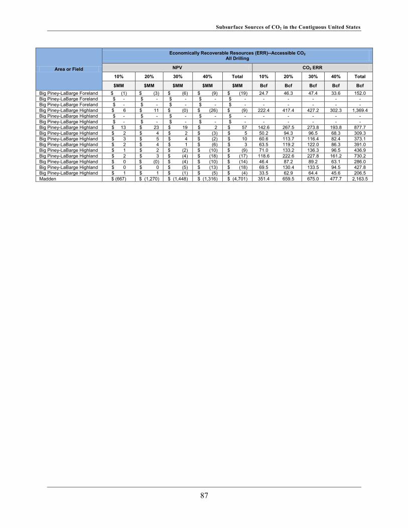
Subsurface Sources of CO2 in the Contiguous United States
Area or Field
Economically Recoverable Resources (ERR)--Accessible CO2 All Drilling
NPV CO2 ERR
10% 20% 30% 40% Total 10% 20% 30% 40% Total
$MM $MM $MM $MM $MM Bcf Bcf Bcf Bcf Bcf Big Piney-LaBarge Foreland $ (1) $ (3) $ (6) $ (9) $ (19) 24.7 46.3 47.4 33.6 152.0 Big Piney-LaBarge Foreland $ - $ - $ - $ - $ - - - - - - Big Piney-LaBarge Foreland $ - $ - $ - $ - $ - - - - - - Big Piney-LaBarge Highland $ 6 $ 11 $ (0) $ (26) $ (9) 222.4 417.4 427.2 302.3 1,369.4 Big Piney-LaBarge Highland $ - $ - $ - $ - $ - - - - - - Big Piney-LaBarge Highland $ - $ - $ - $ - $ - - - - - - Big Piney-LaBarge Highland $ 13 $ 23 $ 19 $ 2 $ 57 142.6 267.5 273.8 193.8 877.7 Big Piney-LaBarge Highland $ 2 $ 4 $ 2 $ (3) $ 5 50.2 94.3 96.5 68.3 309.3 Big Piney-LaBarge Highland $ 3 $ 5 $ 4 $ (2) $ 10 60.6 113.7 116.4 82.4 373.1 Big Piney-LaBarge Highland $ 2 $ 4 $ 1 $ (6) $ 3 63.5 119.2 122.0 86.3 391.0 Big Piney-LaBarge Highland $ 1 $ 2 $ (2) $ (10) $ (9) 71.0 133.2 136.3 96.5 436.9 Big Piney-LaBarge Highland $ 2 $ 3 $ (4) $ (18) $ (17) 118.6 222.6 227.8 161.2 730.2 Big Piney-LaBarge Highland $ 0 $ (0) $ (4) $ (10) $ (14) 46.4 87.2 89.2 63.1 286.0 Big Piney-LaBarge Highland $ 0 $ 0 $ (5) $ (13) $ (18) 69.5 130.4 133.5 94.5 427.8 Big Piney-LaBarge Highland $ 1 $ 1 $ (1) $ (5) $ (4) 33.5 62.9 64.4 45.6 206.5 Madden $ (667) $ (1,270) $ (1,448) $ (1,316) $ (4,701) 351.4 659.5 675.0 477.7 2,163.5
87
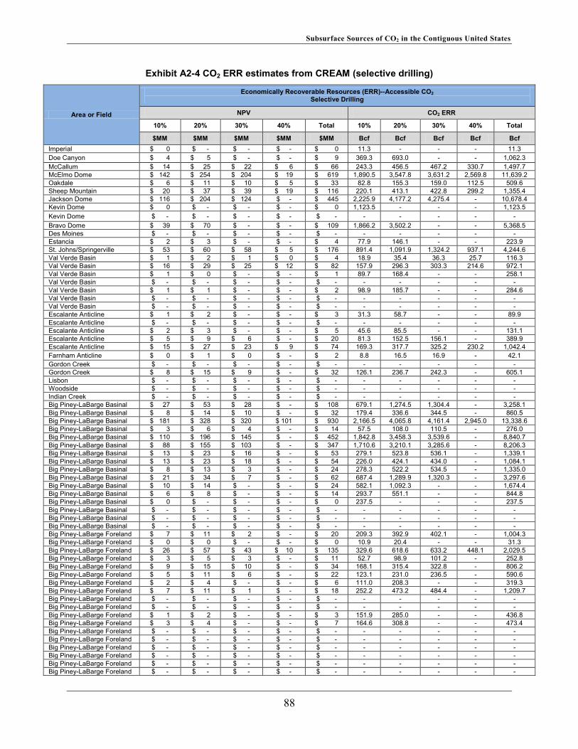
Subsurface Sources of CO2 in the Contiguous United States
Exhibit A2-4 CO2 ERR estimates from CREAM (selective drilling)
Area or Field
Economically Recoverable Resources (ERR)--Accessible CO2 Selective Drilling
NPV CO2 ERR
10% 20% 30% 40% Total 10% 20% 30% 40% Total
$MM $MM $MM $MM $MM Bcf Bcf Bcf Bcf Bcf Imperial $ 0 $ - $ - $ - $ 0 11.3 - - - 11.3 Doe Canyon $ 4 $ 5 $ - $ - $ 9 369.3 693.0 - - 1,062.3 McCallum $ 14 $ 25 $ 22 $ 6 $ 66 243.3 456.5 467.2 330.7 1,497.7 McElmo Dome $ 142 $ 254 $ 204 $ 19 $ 619 1,890.5 3,547.8 3,631.2 2,569.8 11,639.2 Oakdale $ 6 $ 11 $ 10 $ 5 $ 33 82.8 155.3 159.0 112.5 509.6 Sheep Mountain $ 20 $ 37 $ 39 $ 19 $ 116 220.1 413.1 422.8 299.2 1,355.4 Jackson Dome $ 116 $ 204 $ 124 $ - $ 445 2,225.9 4,177.2 4,275.4 - 10,678.4 Kevin Dome $ 0 $ - $ - $ - $ 0 1,123.5 - - - 1,123.5 Kevin Dome $ - $ - $ - $ - $ - - - - - - Bravo Dome $ 39 $ 70 $ - $ - $ 109 1,866.2 3,502.2 - - 5,368.5 Des Moines $ - $ - $ - $ - $ - - - - - - Estancia $ 2 $ 3 $ - $ - $ 4 77.9 146.1 - - 223.9 St. Johns/Springerville $ 53 $ 60 $ 58 $ 5 $ 176 891.4 1,091.9 1,324.2 937.1 4,244.6 Val Verde Basin $ 1 $ 2 $ 1 $ 0 $ 4 18.9 35.4 36.3 25.7 116.3 Val Verde Basin $ 16 $ 29 $ 25 $ 12 $ 82 157.9 296.3 303.3 214.6 972.1 Val Verde Basin $ 1 $ 0 $ - $ - $ 1 89.7 168.4 - - 258.1 Val Verde Basin $ - $ - $ - $ - $ - - - - - - Val Verde Basin $ 1 $ 1 $ - $ - $ 2 98.9 185.7 - - 284.6 Val Verde Basin $ - $ - $ - $ - $ - - - - - - Val Verde Basin $ - $ - $ - $ - $ - - - - - - Escalante Anticline $ 1 $ 2 $ - $ - $ 3 31.3 58.7 - - 89.9 Escalante Anticline $ - $ - $ - $ - $ - - - - - - Escalante Anticline $ 2 $ 3 $ - $ - $ 5 45.6 85.5 - - 131.1 Escalante Anticline $ 5 $ 9 $ 6 $ - $ 20 81.3 152.5 156.1 - 389.9 Escalante Anticline $ 15 $ 27 $ 23 $ 9 $ 74 169.3 317.7 325.2 230.2 1,042.4 Farnham Anticline $ 0 $ 1 $ 0 $ - $ 2 8.8 16.5 16.9 - 42.1 Gordon Creek $ - $ - $ - $ - $ - - - - - - Gordon Creek $ 8 $ 15 $ 9 $ - $ 32 126.1 236.7 242.3 - 605.1 Lisbon $ - $ - $ - $ - $ - - - - - - Woodside $ - $ - $ - $ - $ - - - - - - Indian Creek $ - $ - $ - $ - $ - - - - - - Big Piney-LaBarge Basinal $ 27 $ 53 $ 28 $ - $ 108 679.1 1,274.5 1,304.4 - 3,258.1 Big Piney-LaBarge Basinal $ 8 $ 14 $ 10 $ - $ 32 179.4 336.6 344.5 - 860.5 Big Piney-LaBarge Basinal $ 181 $ 328 $ 320 $ 101 $ 930 2,166.5 4,065.8 4,161.4 2,945.0 13,338.6 Big Piney-LaBarge Basinal $ 3 $ 6 $ 4 $ - $ 14 57.5 108.0 110.5 - 276.0 Big Piney-LaBarge Basinal $ 110 $ 196 $ 145 $ - $ 452 1,842.8 3,458.3 3,539.6 - 8,840.7 Big Piney-LaBarge Basinal $ 88 $ 155 $ 103 $ - $ 347 1,710.6 3,210.1 3,285.6 - 8,206.3 Big Piney-LaBarge Basinal $ 13 $ 23 $ 16 $ - $ 53 279.1 523.8 536.1 - 1,339.1 Big Piney-LaBarge Basinal $ 13 $ 23 $ 18 $ - $ 54 226.0 424.1 434.0 - 1,084.1 Big Piney-LaBarge Basinal $ 8 $ 13 $ 3 $ - $ 24 278.3 522.2 534.5 - 1,335.0 Big Piney-LaBarge Basinal $ 21 $ 34 $ 7 $ - $ 62 687.4 1,289.9 1,320.3 - 3,297.6 Big Piney-LaBarge Basinal $ 10 $ 14 $ - $ - $ 24 582.1 1,092.3 - - 1,674.4 Big Piney-LaBarge Basinal $ 6 $ 8 $ - $ - $ 14 293.7 551.1 - - 844.8 Big Piney-LaBarge Basinal $ 0 $ - $ - $ - $ 0 237.5 - - - 237.5 Big Piney-LaBarge Basinal $ - $ - $ - $ - $ - - - - - - Big Piney-LaBarge Basinal $ - $ - $ - $ - $ - - - - - - Big Piney-LaBarge Basinal $ - $ - $ - $ - $ - - - - - - Big Piney-LaBarge Foreland $ 7 $ 11 $ 2 $ - $ 20 209.3 392.9 402.1 - 1,004.3 Big Piney-LaBarge Foreland $ 0 $ 0 $ - $ - $ 0 10.9 20.4 - - 31.3 Big Piney-LaBarge Foreland $ 26 $ 57 $ 43 $ 10 $ 135 329.6 618.6 633.2 448.1 2,029.5 Big Piney-LaBarge Foreland $ 3 $ 5 $ 3 $ - $ 11 52.7 98.9 101.2 - 252.8 Big Piney-LaBarge Foreland $ 9 $ 15 $ 10 $ - $ 34 168.1 315.4 322.8 - 806.2 Big Piney-LaBarge Foreland $ 5 $ 11 $ 6 $ - $ 22 123.1 231.0 236.5 - 590.6 Big Piney-LaBarge Foreland $ 2 $ 4 $ - $ - $ 6 111.0 208.3 - - 319.3 Big Piney-LaBarge Foreland $ 7 $ 11 $ 1 $ - $ 18 252.2 473.2 484.4 - 1,209.7 Big Piney-LaBarge Foreland $ - $ - $ - $ - $ - - - - - - Big Piney-LaBarge Foreland $ - $ - $ - $ - $ - - - - - - Big Piney-LaBarge Foreland $ 1 $ 2 $ - $ - $ 3 151.9 285.0 - - 436.8 Big Piney-LaBarge Foreland $ 3 $ 4 $ - $ - $ 7 164.6 308.8 - - 473.4 Big Piney-LaBarge Foreland $ - $ - $ - $ - $ - - - - - - Big Piney-LaBarge Foreland $ - $ - $ - $ - $ - - - - - - Big Piney-LaBarge Foreland $ - $ - $ - $ - $ - - - - - - Big Piney-LaBarge Foreland $ - $ - $ - $ - $ - - - - - - Big Piney-LaBarge Foreland $ - $ - $ - $ - $ - - - - - - Big Piney-LaBarge Foreland $ - $ - $ - $ - $ - - - - - -
88

Subsurface Sources of CO2 in the Contiguous United States
Area or Field
Economically Recoverable Resources (ERR)--Accessible CO2 Selective Drilling
NPV CO2 ERR
10% 20% 30% 40% Total 10% 20% 30% 40% Total
$MM $MM $MM $MM $MM Bcf Bcf Bcf Bcf Bcf Big Piney-LaBarge Foreland $ - $ - $ - $ - $ - - - - - - Big Piney-LaBarge Foreland $ - $ - $ - $ - $ - - - - - - Big Piney-LaBarge Foreland $ - $ - $ - $ - $ - - - - - - Big Piney-LaBarge Highland $ 6 $ 11 $ - $ - $ 17 222.4 417.4 - - 639.8 Big Piney-LaBarge Highland $ - $ - $ - $ - $ - - - - - - Big Piney-LaBarge Highland $ - $ - $ - $ - $ - - - - - - Big Piney-LaBarge Highland $ 13 $ 23 $ 19 $ 2 $ 57 142.6 267.5 273.8 193.8 877.7 Big Piney-LaBarge Highland $ 2 $ 4 $ 2 $ - $ 9 50.2 94.3 96.5 - 241.0 Big Piney-LaBarge Highland $ 3 $ 5 $ 4 $ - $ 12 60.6 113.7 116.4 - 290.7 Big Piney-LaBarge Highland $ 2 $ 4 $ 1 $ - $ 8 63.5 119.2 122.0 - 304.7 Big Piney-LaBarge Highland $ 1 $ 2 $ - $ - $ 3 71.0 133.2 - - 204.1 Big Piney-LaBarge Highland $ 2 $ 3 $ - $ - $ 5 118.6 222.6 - - 341.2 Big Piney-LaBarge Highland $ 0 $ - $ - $ - $ 0 46.4 - - - 46.4 Big Piney-LaBarge Highland $ 0 $ 0 $ - $ - $ 0 69.5 130.4 - - 199.9 Big Piney-LaBarge Highland $ 1 $ 1 $ - $ - $ 2 33.5 62.9 - - 96.5 Madden $ - $ - $ - $ - $ - - - - - -
89

www.netl.doe.gov
Pittsburgh, PA • Morgantown, WV • Albany, OR • Sugar Land, TX • Anchorage, AK
(800) 553-7681
Robert Wallace [email protected]
Phil DiPietro [email protected]
Jeffrey Eppink [email protected]


![PAINTINGS [ODETTE LABARGE]](https://img.pdfslide.us/doc/110x75/55d49c95bb61ebaa2c8b4589/paintings-odette-labarge.jpg)


![LABARGE DESIGN PROFILE [PORTFOLIIO]](https://img.pdfslide.us/doc/110x75/54b339794a79594e7d8b4584/labarge-design-profile-portfoliio.jpg)