Off-road Path Following using Region Classification and Geometric ProjectionConstraints∗

Yaniv AlonMobileye Ltd.

Jerusalem, Israel

Andras FerenczMobileye Ltd.

Jerusalem, Israel

Amnon ShashuaSchool of Eng. and CS

The Hebrew University of Jerusalem

Abstract

We describe a realtime system for finding and trackingunstructured paths in off-road conditions. The system wasdesigned as part of the recent Darpa Grand Challenge andwas tested over hundreds of miles of off-road driving. Theunique feature of our approach is to combine geometricprojection used for recovering Pitch and Yaw with Learn-ing approaches for identifying familiar ”drivable” regionsin the scene. The region-based component segments theimage to ”path” and ”non-path” regions based on tex-ture analysis borne out of a learning-by-examples principle.The boundary-based component looks for the path bound-ing lines assuming a geometric model of a planar pathwaybounded by parallel edges taken by a perspective camera.The combined effect of both sub-systems forms a robust sys-tem capable of finding the path even in situations where thevehicle is positioned out of the path — a situation whichis not common for human drivers but is relevant for au-tonomous driving where the vehicle may find itself occa-sionally veering out of the path.

1. Introduction

The interest in paved and unstructured road/path follow-ing has attracted interest for more than two decades withearly systems focused on paved road following [3, 12] (seealso survey in [2]) and more recent attempts to handle off-road conditions — some of it triggered by the races of theDarpa Grand Challenge off-road autonomous driving com-petitions [4] held in 2004 and 2005 in the Mojave desert —[10, 1, 9, 13, 15].

Paved road following is largely considered a ”solved”problem as a growing number of automotive manufactur-ers are offering lane departure warning systems. However,off-road path detection and following poses several interest-

∗This work is part of Yaniv Alon’s MSc dissertation completed at theHebrew University. Andras Ferencz was at UC Bekeley during the timewhen this work was completed.

(a) (b)

(c) (d)

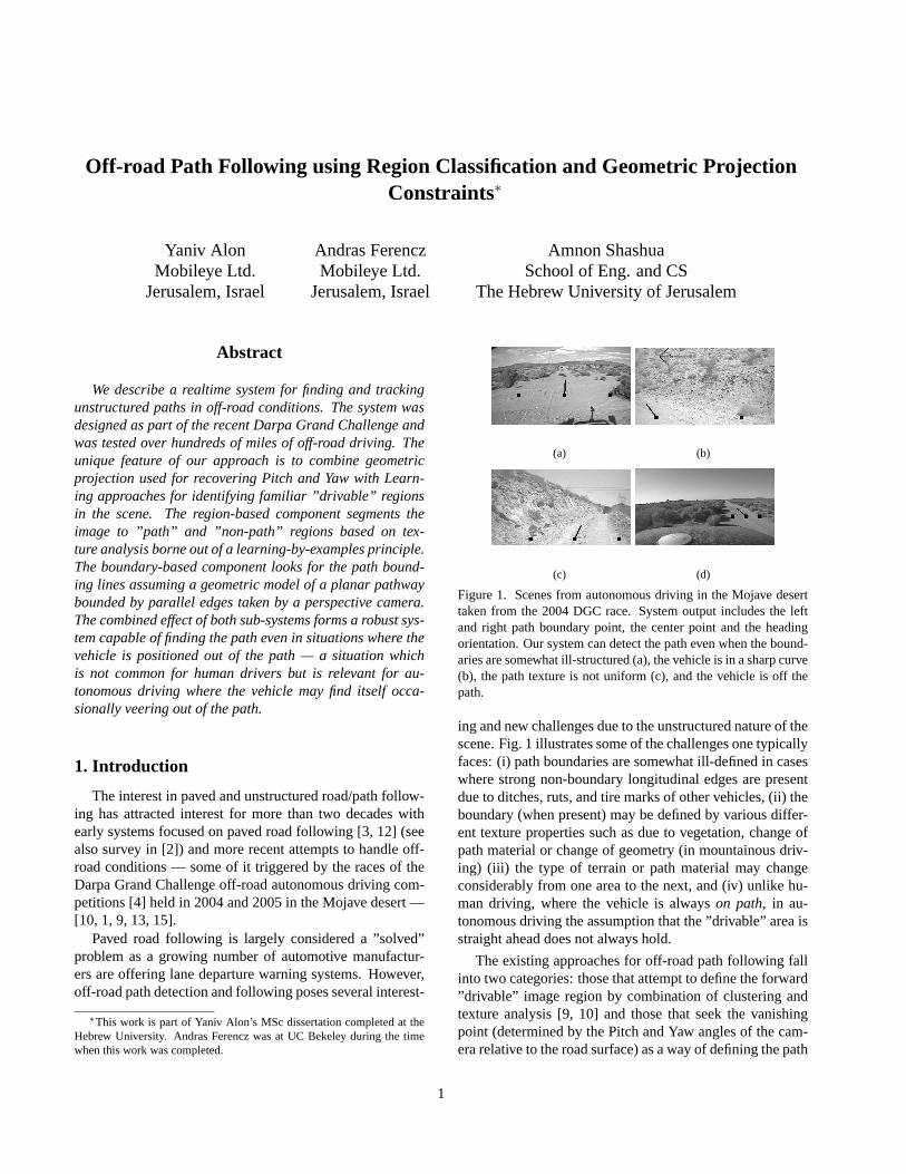
Figure 1. Scenes from autonomous driving in the Mojave deserttaken from the 2004 DGC race. System output includes the leftand right path boundary point, the center point and the headingorientation. Our system can detect the path even when the bound-aries are somewhat ill-structured (a), the vehicle is in a sharp curve(b), the path texture is not uniform (c), and the vehicle is off thepath.

ing and new challenges due to the unstructured nature of thescene. Fig.1 illustrates some of the challenges one typicallyfaces: (i) path boundaries are somewhat ill-defined in caseswhere strong non-boundary longitudinal edges are presentdue to ditches, ruts, and tire marks of other vehicles, (ii) theboundary (when present) may be defined by various differ-ent texture properties such as due to vegetation, change ofpath material or change of geometry (in mountainous driv-ing) (iii) the type of terrain or path material may changeconsiderably from one area to the next, and (iv) unlike hu-man driving, where the vehicle is alwayson path, in au-tonomous driving the assumption that the ”drivable” area isstraight ahead does not always hold.

The existing approaches for off-road path following fallinto two categories: those that attempt to define the forward”drivable” image region by combination of clustering andtexture analysis [9, 10] and those that seek the vanishingpoint (determined by the Pitch and Yaw angles of the cam-era relative to the road surface) as a way of defining the path

1

boundaries [15]. The first approach lacks a geometric modelof the path which can be described by a small number of pa-rameters assuming that the path ahead is planar and viewedby a perspective projection, whereas the second approachfocuses only on detecting boundaries (which when behavedcorrectly could vote towards the position of the vanishingpoint) and ignores the ”region-based” nature of the path.Both approaches have their pros and cons but neither singleapproach can handle the full extent of the required off-roadchallenge.

In our work we propose combining a region-based clas-sification subsystem of image texture to ”path” and ”non-path” regions together with a geometric subsystem consist-ing of a flat world assumption taken from a perspective pro-jection for finding the path boundary lines. Both subsys-tems complement each other thus combining the strengthsof both the region-based and boundary-based approaches.Specifically, we use a variety of texture filters together witha learning-by-examples Adaboost [6] classification engineto form an initial image segmentation into Path and Non-path image blocks. Independently, we use the same filtersto define candidate texture boundaries and use a projection-warp search over the space of possible Pitch and Yaw pa-rameters in order to select a pair of boundary lines whichare consistent with both the texture gradients and the geo-metric model. The area-based and boundary-based modulesare then weighted by their confidence values to form a finalpath model for each frame.

The system was implemented on a Power-PC PPC74671GHZ running at 20 frames per second. We have run thesystem successfully on 6 hours of recorded data of the en-tire 2004 DGC race and completed successfully around50miles of the 2005 race — both held in the Mojave desert[4]. The 2005 GDC race was in cooperation with theGolem/UCLA group — the vehicle platform can be seenin Fig. 2.

2. Feature Measurements for Classificationand Boundary Detection

As mentioned above, our system combines two modules— region-based and boundary based — working in tandem.The region based module classifies image blocks into Pathand Non-path labels based on a learning training set and theboundary-based module fits a geometric camera constrainton the boundaries of the path. Both modules require meansfor measuring texture features — either to be later fed intoa classifier or as a basis for deciding where the boundariesbetween the path and non-path regions may reside. In thissection we briefly describe three different feature extractionschemes we used during research including oriented filters,Walsh-Hadamard kernels and Moments.

Figure 2. The Golem/UCLA group vehicle used as our test plat-form. In this installation the camera is mounted inside a housingon top of a pole connected to the front bumper. Other installationshad the camera mounted on the windshield.

Oriented Gaussian Derivatives Filters We consideredan oriented Gaussian Derivatives filter bank similar to theone used by Maliket al. [11] for partitioning grayscale im-ages into disjoint regions with coherent brightness and tex-ture. For a given scaleσ, the filter bank contains even andodd-symmetric filters

godd(x, y, σ) =d2

dy2(exp(

y2

2σ2) exp(

x2

l22σ2)) (1)

geven(x, y, σ) = Hilbert(godd(x, y, σ)) (2)

and one center-surround filter

cs(x, y, σ) = exp(y2

1.52σ2) exp(

x2

1.52σ2)

−exp( y2

0.52σ2) exp(

x2

0.52σ2

The coefficientl = 3 is the aspect ratio between the two1D Gaussians that form a quadrature pair ([5]) godd andgeven , i.e., having the same frequency response but differin phase. The actual filter bank contains zero-mean versionsgodd, geven, cs normalized to unitL1 norm. For a givenscaleσ, the filter bank contains rotated versions ofgodd andgeven in four equally spaced orientations, and onecs filterwhich makes it a total of nine filters per scale. The filterresponse around each filter is calculated with two scales ad-justed to the row position due to foreshortening (total of18responses per pixel).

Walsh-Hadamard Kernels The Gaussian derivatives fil-ter bank forms a computationally expensive approach whichcould be prohibitive for a realtime system. We consideredusing as an alternative a fast convolution approach based on

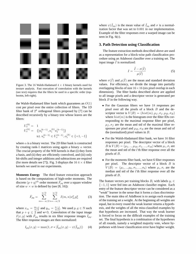
Figure 3. The16 Walsh-Hadamard4 × 4 binary kernels used fortexture analysis. Fast execution of convolution with the kernels(see text) requires that the filters be used in a specific order (top-bootm, left-right).

the Walsh-Hadamard filter bank which guarantees anO(1)cost per pixel over the entire collection of filters. The 1Dfilter bank of2k orthogonal filters proposed by [7] can bedescribed recursively by a binary tree whose leaves are thefilters:

U(0)s = 1

U(k)s = {[u(k−1)

s , α(k)i u(k−1)

s ]}

s.t.u(k−1)s ∈ U (k−1)

s , α(k)i ∈ {+1,−1}

whereα is a binary vector. The 2D filter bank is constructedby creating rank-1 matrices using again a binaryα vector.The crucial property of the WH kernels is that (i) they forma basis, and (ii) they are efficiently convolved, and (iii) onlybit-shifts and integer additions and subtractions are required(for more details see [7]). Fig. 3 displays the16 4× 4 filterkernels we used in our experiments.

Moments Energy The third feature extraction approachis based on the computations of high-order moments. Thediscrete(p+ q)th order momentFpq over a square windowof sizew × w is defined by (see [8, 16]):

Fpq =w/2∑

m=−w/2

w/2∑n=−w/2

I(m,n)xpmy

qn (3)

wherexm = m−iw/2 andym = n−j

w/2 . We usedp, q ∈ N suchthat p + q ≤ 2 and w=3. Convolution of the input imageI(x, y) with Fpq results in six filter response imagesIpq.The filter response images are then normalized:

Ipq(x, y) = max(1, σ ∗ |Ipq(x, y)− ψ(Ipq)|) (4)

whereψ(Ipq) is the mean value ofIpq andσ is a normal-ization factor that was set to0.001 in our implementation.Example of the filter responses over a warped image can beseen in Fig.6(c).

3. Path Detection using Classification

The feature extraction methods described above are usedas a representation for a block-wise path classification pro-cedure using an Adaboost classifier over a training set. Theinput imageI is normalized:

I =I − σ(I)µ(I)

(5)

whereσ(I) andµ(I) are the mean and standard deviationvalues. For efficiency, we divide the image into partiallyoverlapping blocks of size16×16 (six pixel overlap in eachdimension). The filter banks described above are appliedto all image pixels and a descriptor vector is generated perblockB in the following way.

• For the Gaussian filters we have18 responses perpixel over all the pixels of a blockB and the de-scriptor vector isV (B) = (hist(m), µf , σf , µB , σB)wherehist(m) is the histogram over the filter IDs cor-responding to the maximal response filter per pixel,µf , σf are the mean and std of the maximal filter re-sponses per pixel andµB , σB are the mean and std ofthe (normalized) pixel values inB.

• For the Walsh-Hadamard filter bank, we have16 filterresponses per pixel. The descriptor vector of a blockB is V (B) = (µ1, .., µ16, σ1, ..., σ16) whereµi, σi arethe mean and std of the i’th filter response over all thepixels ofB.

• For the moments filter bank, we have 6 filter responsesper pixel. The descriptor vector of a blockB isV (B) = (µ1, .., µ6, σ1, ..., σ6) whereµi, σi are themedian and std of the i’th filter response over all thepixels ofB.

The feature vectors per training blocksBi with labelsyi ∈{−1, 1} were fed into an Adaboost classifier engine. Eachentry of the feature descriptor vector can be considered as a”weak” learner in the sense that it forms a class discrimina-tion. The main idea of AdaBoost is to assign each exampleof the training set a weight. At the beginning all weights areequal, but in every round the weak learner returns a hypoth-esis, and the weights of all the miss-classified examples bythat hypothesis are increased. That way the weak learneris forced to focus on the difficult examples of the trainingset. The final hypothesis is a combination of the hypothesesof all rounds, namely a weighted majority vote, where hy-potheses with lower classification error have higher weight.

0 5 10 15 20 25 30 35 40 45 500.78

0.79

0.8

0.81

0.82

0.83

0.84

0.85

0.86

0.87

0.88

AdaBoost iteration index

clas

sific

atio

n ac

cura

cy

Gausian filters, AdaboostWH filters of size 4x4, AdaboostWH filters of size 4x4, SVMGausian filters, SVMMoments filters, Adaboost

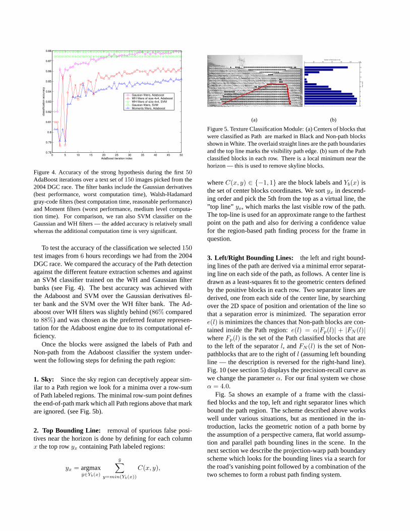
Figure 4. Accuracy of the strong hypothesis during the first50AdaBoost iterations over a text set of150 images picked from the2004 DGC race. The filter banks include the Gaussian derivatives(best performance, worst computation time), Walsh-Hadamardgray-code filters (best computation time, reasonable performance)and Moment filters (worst performance, medium level computa-tion time). For comparison, we ran also SVM classifier on theGaussian and WH filters — the added accuracy is relatively smallwhereas the additional computation time is very significant.

To test the accuracy of the classification we selected150test images from6 hours recordings we had from the 2004DGC race. We compared the accuracy of the Path detectionagainst the different feature extraction schemes and againstan SVM classifier trained on the WH and Gaussian filterbanks (see Fig.4). The best accuracy was achieved withthe Adaboost and SVM over the Gaussian derivatives fil-ter bank and the SVM over the WH filter bank. The Ad-aboost over WH filters was slightly behind (86% comparedto 88%) and was chosen as the preferred feature represen-tation for the Adaboost engine due to its computational ef-ficiency.

Once the blocks were assigned the labels of Path andNon-path from the Adaboost classifier the system under-went the following steps for defining the path region:

1. Sky: Since the sky region can deceptively appear sim-ilar to a Path region we look for a minima over a row-sumof Path labeled regions. The minimal row-sum point definesthe end-of-path mark which all Path regions above that markare ignored. (see Fig.5b).

2. Top Bounding Line: removal of spurious false posi-tives near the horizon is done by defining for each columnx the top rowyx containing Path labeled regions:

yx = argmaxy∈Yb(x)

y∑y=min(Yb(x))

C(x, y),

(a)

0 20 40 60 80 100 120

0

2

4

6

8

10

12

14

16

18

Number of Path blocks in row

Row

inde

x

(b)

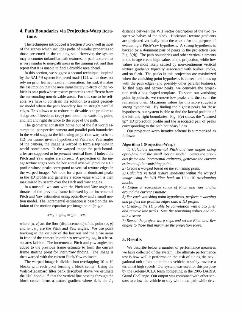
Figure 5. Texture Classification Module: (a) Centers of blocks thatwere classified as Path are marked in Black and Non-path blocksshown in White. The overlaid straight lines are the path boundariesand the top line marks the visibility path edge. (b) sum of the Pathclassified blocks in each row. There is a local minimum near thehorizon — this is used to remove skyline blocks.

whereC(x, y) ∈ {−1, 1} are the block labels andYb(x) isthe set of center blocks coordinates. We sortyx in descend-ing order and pick the 5th from the top as a virtual line, the”top line” yo, which marks the last visible row of the path.The top-line is used for an approximate range to the farthestpoint on the path and also for deriving a confidence valuefor the region-based path finding process for the frame inquestion.

3. Left/Right Bounding Lines: the left and right bound-ing lines of the path are derived via a minimal error separat-ing line on each side of the path, as follows. A center line isdrawn as a least-squares fit to the geometric centers definedby the positive blocks in each row. Two separator lines arederived, one from each side of the center line, by searchingover the 2D space of position and orientation of the line sothat a separation error is minimized. The separation errore(l) is minimizes the chances that Non-path blocks are con-tained inside the Path region:e(l) = α|Fp(l)| + |FN (l)|whereFp(l) is the set of the Path classified blocks that areto the left of the separatorl, andFN (l) is the set of Non-pathblocks that are to the right ofl (assuming left boundingline — the description is reversed for the right-hand line).Fig. 10(see section5) displays the precision-recall curve aswe change the parameterα. For our final system we choseα = 4.0.

Fig. 5a shows an example of a frame with the classi-fied blocks and the top, left and right separator lines whichbound the path region. The scheme described above workswell under various situations, but as mentioned in the in-troduction, lacks the geometric notion of a path borne bythe assumption of a perspective camera, flat world assump-tion and parallel path bounding lines in the scene. In thenext section we describe the projection-warp path boundaryscheme which looks for the bounding lines via a search forthe road’s vanishing point followed by a combination of thetwo schemes to form a robust path finding system.

4. Path Boundaries via Projection-Warp itera-tions

The techniques introduced is Section3work well in mostof the scenes which includes paths of similar properties tothose presented in the training set. However, the systemmay encounter unfamiliar path textures, or path texture thatis very similar to non-path areas in the training set, and thusreport that it is unable to find a drivable area ahead.

In this section, we suggest a second technique, inspiredby the RALPH system for paved roads [12], which does notrely on prior learned texture information. Instead, it makesthe assumption that the area immediately in-front of the ve-hicle is on a path whose texture properties are different fromthe surrounding non-drivable areas. For this cue to be reli-able, we have to constrain the solution to a strict geomet-ric model where the path boundary lies on straight paralleledges. This allows us to reduce the drivable path problem to4 degrees of freedom:(x, y) position of the vanishing point,and left and right distance to the edge of the path.

The geometric constraint borne out of the flat world as-sumption, perspective camera and parallel path boundariesin the world suggest the following projection-warp scheme[12] per frame: given a hypothesis of Pitch and Yaw anglesof the camera, the image is warped to form a top view inworld coordinates. In the warped image the path bound-aries are supposed to beparallel vertical lines if indeed thePitch and Yaw angles are correct. A projection of the im-age texture edges onto the horizontal axis will produce a 1Dprofile whose peaks correspond to vertical texture edges inthe warped image. We look for a pair of dominant peaksin the 1D profile and generate a score value which is thenmaximized by search over the Pitch and Yaw angles.

In a nutshell, we start with the Pitch and Yaw angle es-timates of the previous frame followed by an incrementalPitch and Yaw estimation using optic-flow and a small mo-tion model. The incremental estimation is based on the so-lution of the motion equation per image point(x, y):

xwx + ywy = yu− xv,

where(u, v) are the flow (displacements) of the point(x, y)andwx, wy are the Pitch and Yaw angles. We use pointtracking in the vicinity of the horizon and the close areasin front of the camera in order to recoverwx, wy in a least-squares fashion. The incremental Pitch and yaw angles areadded to the previous frame estimate to form the currentframe starting point for Pitch/Yaw finding. The image isthen warped with the current Pitch/Yaw estimate.

The warped image is divided into overlapping10 × 10blocks with each pixel forming a block center. Using theWalsh-Hadamard filter bank described above we estimatethe likelihoode−∆ that the vertical line passing through theblock center forms a texture gradient where∆ is theL1

distance between the WH vector descriptors of the two re-spective halves of the block. Horizontal texture gradientsare projected vertically onto thex-axis for the purpose ofevaluating a Pitch/Yaw hypothesis. A strong hypothesis isbacked by a dominant pair of peaks in the projection (seeFig. 6(d)). The path boundaries and other vertical elementsin the image create high values in the projection, while lowvalues are most likely caused by non-continuous verticaltexture gradients typically associated with bushes, rocks,and so forth. The peaks in this projection are maximizedwhen the vanishing point hypothesis is correct and lines upwith the path edges (and possibly other parallel features).To find high and narrow peaks, we convolve the projec-tion with a box-shaped template. To score our vanishingpoint hypothesis, we remove low peaks and then sum theremaining ones. Maximum values for this score suggest astrong hypothesis. By finding the highest peaks for thesehypotheses, our system is able to find the lateral position ofthe left and right boundaries. Fig.6(e)shows the ”cleanedup” 1D projection profile and the associated pair of peakscorresponding to the path boundary lines.

Our projection-warp iterative scheme is summarized asfollows:

Algorithm 1 (Projection-Warp)1) Calculate incremental Pitch and Yaw angles using

optic-flow and the small motion model. Using the previ-ous frame and incremental estimates, generate the currentestimate of the vanishing point.2) Create a warped based on the vanishing point.3) Calculate vertical texture gradients within the warpedimage using the WH filter bank on10 × 10 overlappingblocks.4) Define a reasonable range of Pitch and Yaw anglesaround the current estimate.5) For each vanishing point hypothesis, perform a warpingand project the gradient edges onto a 1D profile.6) Clean-up the 1D profile by convolution with a box filterand remove low peaks. Sum the remaining values and ob-tain a score.7) Repeat the project-warp steps and set the Pitch and Yawangles to those that maximize the projection score.

5. Results

We describe below a number of performance measureswe have collected of the system. The ultimate performancetest is how well it performs on the task of aiding the navi-gational unit of an autonomous vehicle to safely traverse aterrain at high speeds. Our system was used for this purposeby the Golem/UCLA team competing in the 2005 DARPAGrand Challenge. Our output was combined with other sen-sors to allow the vehicle to stay within the path while driv-

(a) (b) (c)

(d) (e)

Figure 6. Projection-Warp Search: (a) original image with theoverlaid path boundary and vanishing point results. (b) the warpedimage. (c) texture gradients magnitude. (d) projection: verticalsum of gradients. (e) projection profile followed by convolutionwith a box filter. The two lines on top of the histogram marks thepath boundaries.

ing at speeds up to50 mph on straight segments as well asto navigate mountainous trails.

(a) (b) (c)

(d) (e) (f)

(g) (h) (i)

Figure 7. Sample images and system output from 6 hours of driv-ing in the Mojave desert (2004 DGC race). The path is markedby two left-right boundary points and a center point with headingorientation. The ”X” mark in (h) coincides with Zero confidence(i.e., system deactivates momentarily) due to confusion with mul-tiple shadows. In (i) the path is detected even though the vehicleis not centered on the path (a situation which is common for au-tonomous driving).

Our system was trained over 200 randomly selected im-ages from 6 hours of video over 140 miles of trails in theMojave desert covering the course of DARPA Grand Chal-lenge 2004. The trails cover a large variety of terrain types

(a) (b) (c)

(d) (e) (f)

Figure 8. The Path /Non-path texture classification (a),(d) is fol-lowed by sky blocks removal and by fitting three lines (arrangedas a trapezoid) to the Path blocks. In (b),(e) all the blocks withinthe trapezoid are labeled as Path, and all the others as Non-path.Finally, the path boundaries at a given distance is calculated (c),(f)together with the path center and heading angle.

including sandy straight paths, gravel covered winding trailsand rocky mountain passes. The video was recorded with acamera located inside the cabin and mounted on the wind-shield near the rearview mirror. A field of view of 45 de-grees was used during training but during the 2005 DGCrace a wider field of view of 80 degrees was adopted. Fol-lowing the training phase, we tested the system performanceon the original 6 hours of video with a 45 degrees FOV andwith one hour of video recorded with an 80 degrees FOV.Sample images of the system output during these tests areshown in Fig.7, while Fig. 8 shows the results of each ofthe main parts of the classification based algorithm.

Overall performance. The most meaningful overallsystem performance measure is to count how often (whatfraction of frames) the system produced correct path edgepositions and, where appropriate, heading angles. Further-more, it is crucial for the system to know when it can notdetermine the path accurately, so that the vehicle can slowdown and rely more on information from other sensors. Ourresults are broken down to different terrain types. For each,representative challenging clips of 1000 frames were se-lected (see Fig.9) and the system performance scored onthose sequences by a human observer. The path edge dis-tance accuracy was computed by observing the position ofthe road edge marks approximately 6 meters in front of thevehicle. A frame was labeled incorrect if the path edgemarker at that location appeared to be more then 30 cm(≈ 18 pixels) away from the actual path boundary. Forstraight paths the perceived vanishing point of the path wasalso marked, and our algorithm’s heading indicator wascompared to the lateral position of that point.

A. On relatively straight segments with a comfortablywide path, the navigation system allows the vehicle to driveat speeds up to50 mph. For those type of scenes (clip (a) in

(a) (b)

(c) (d)

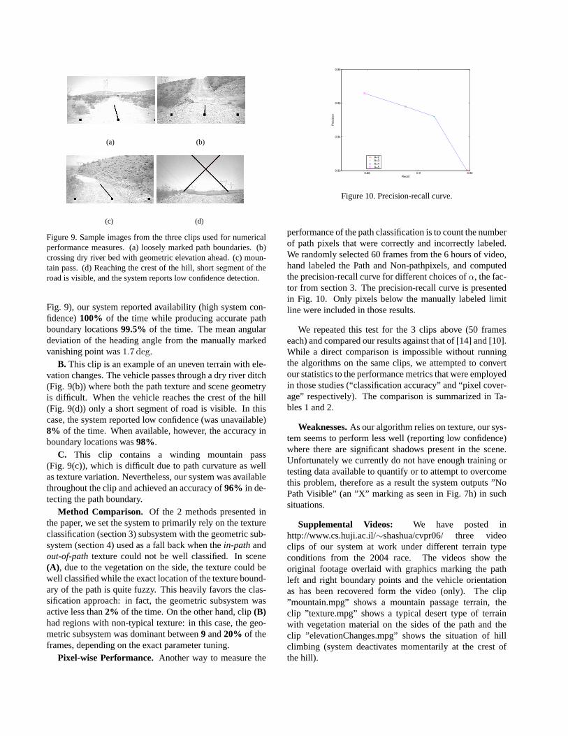
Figure 9. Sample images from the three clips used for numericalperformance measures. (a) loosely marked path boundaries. (b)crossing dry river bed with geometric elevation ahead. (c) moun-tain pass. (d) Reaching the crest of the hill, short segment of theroad is visible, and the system reports low confidence detection.

Fig. 9), our system reported availability (high system con-fidence)100% of the time while producing accurate pathboundary locations99.5% of the time. The mean angulardeviation of the heading angle from the manually markedvanishing point was1.7 deg.

B. This clip is an example of an uneven terrain with ele-vation changes. The vehicle passes through a dry river ditch(Fig. 9(b)) where both the path texture and scene geometryis difficult. When the vehicle reaches the crest of the hill(Fig. 9(d)) only a short segment of road is visible. In thiscase, the system reported low confidence (was unavailable)8% of the time. When available, however, the accuracy inboundary locations was98%.

C. This clip contains a winding mountain pass(Fig. 9(c)), which is difficult due to path curvature as wellas texture variation. Nevertheless, our system was availablethroughout the clip and achieved an accuracy of96% in de-tecting the path boundary.

Method Comparison. Of the 2 methods presented inthe paper, we set the system to primarily rely on the textureclassification (section3) subsystem with the geometric sub-system (section4) used as a fall back when thein-pathandout-of-pathtexture could not be well classified. In scene(A), due to the vegetation on the side, the texture could bewell classified while the exact location of the texture bound-ary of the path is quite fuzzy. This heavily favors the clas-sification approach: in fact, the geometric subsystem wasactive less than2% of the time. On the other hand, clip(B)had regions with non-typical texture: in this case, the geo-metric subsystem was dominant between9 and20% of theframes, depending on the exact parameter tuning.

Pixel-wise Performance.Another way to measure the

0.88 0.9 0.920.93

0.94

0.95

0.96

Recall

Pre

cisi

on

A=2A=3A=4A=5

Figure 10. Precision-recall curve.

performance of the path classification is to count the numberof path pixels that were correctly and incorrectly labeled.We randomly selected 60 frames from the 6 hours of video,hand labeled the Path and Non-pathpixels, and computedthe precision-recall curve for different choices ofα, the fac-tor from section3. The precision-recall curve is presentedin Fig. 10. Only pixels below the manually labeled limitline were included in those results.

We repeated this test for the 3 clips above (50 frameseach) and compared our results against that of [14] and [10].While a direct comparison is impossible without runningthe algorithms on the same clips, we attempted to convertour statistics to the performance metrics that were employedin those studies (“classification accuracy” and “pixel cover-age” respectively). The comparison is summarized in Ta-bles 1 and 2.

Weaknesses.As our algorithm relies on texture, our sys-tem seems to perform less well (reporting low confidence)where there are significant shadows present in the scene.Unfortunately we currently do not have enough training ortesting data available to quantify or to attempt to overcomethis problem, therefore as a result the system outputs ”NoPath Visible” (an ”X” marking as seen in Fig.7h) in suchsituations.

Supplemental Videos: We have posted inhttp://www.cs.huji.ac.il/∼shashua/cvpr06/ three videoclips of our system at work under different terrain typeconditions from the 2004 race. The videos show theoriginal footage overlaid with graphics marking the pathleft and right boundary points and the vehicle orientationas has been recovered form the video (only). The clip”mountain.mpg” shows a mountain passage terrain, theclip ”texture.mpg” shows a typical desert type of terrainwith vegetation material on the sides of the path and theclip ”elevationChanges.mpg” shows the situation of hillclimbing (system deactivates momentarily at the crest ofthe hill).

Method Classification accuracy

Ours (random set of images) 90.0Rasmussen 88.6

Table 1. Results: Classification accuracy metric.

Road type Pixel coverage

ill-structured boundaries 0.790Ditches, large pitch changes 0.732Winding mountain path 0.881Random set of images 0.822Lieb et al. 0.697

Table 2. Results: Pixel coverage metric.

6. Summary

We have described an off-road path-finding algorithmthat was designed as an aide for autonomous driving aspart of the recent 2005 DGC race. The unique featureof the system is that it incorporates two different detec-tion modalities one based on texture classification of imageinto ”Path” and ”Non-path” regions followed by cleaning-up processes for turning the classification result into a pathwith straight-line boundaries and orientations. The secondmodule (projection-warp search) is based on a geometricapproach governed by camera parameters (Pitch and Yaw),flat world assumption and parallel path boundaries in thescene. The two modules run in parallel and the system out-put is governed by the module with the highest confidence.The texture classification module uses a Walsh-Hadamardfilter bank followed by an Adaboost trained classifier. Theprojection-warp search combines motion estimation for aninitial camera parameters estimation followed by a searchmaximizing the sharpness of peaks in the 1D projection ofthe vertical texture gradients.

Acknowledgement

We thank Stefano Soatto and the entire UCLA andGolem teams for the fruitful cooperation during the 2005DGC race. This work was partly funded by a grant No.0397545 from the Israeli defense ministry.

References

[1] J. Crisman and C. Thorpe. Unscarf, a color vi-sion system for the detection of unstructured roads.In Proceedings of IEEE International Conference onRobotics and Automation, volume 3, pages 2496 –2501, April 1991. 1

[2] G. N. DeSouza and A. C. Kak. Vision for mobilerobot navigation: A survey.IEEE Trans. Pattern Anal.Mach. Intell., 24(2):237–267, 2002.1

[3] E. D. Dickmanns and A. Zapp. Autonomous highspeed road vehicle guidance by computer vision.In R. Isermann, editor,Automatic Control—WorldCongress, 1987: Selected Papers from the 10th Trien-nial World Congress of the International Federationof Automatic Control, pages 221–226, Munich, Ger-many, jul 1987. 1

[4] http://www.darpa.mil/grandchallenge/.1, 2

[5] W. T. Freeman and E. H. Adelson. The design and useof steerable filters.IEEE Trans. Pattern Analysis andMachine Intelligence, 13(9):891–906, 1991.2

[6] Y. Freund and R. E. Schapire. Experiments with anew boosting algorithm. InInternational Conferenceon Machine Learning, pages 148–156, 1996.2

[7] Y. Hel-Or and H. Hel-Or. Real-time pattern matchingusing projection kernels.IEEE Trans. Pattern Anal.Mach. Intell., 27(9):1430–1445, September 2005.3

[8] M. Hu. Visual pattern recognition by moment in-variants. IEEE Trans. Inform. Theory, 8(2):179–187,February 1962.3

[9] D. Kuan, G. Phipps, and A.-C. Hsueh. Autonomousrobotic vehicle road following.IEEE Trans. PatternAnal. Mach. Intell., 10(5):648–658, 1988.1

[10] D. Lieb, A. Lookingbill, and S. Thrun. Adaptive roadfollowing using self-supervised learning and reverseoptical flow. InProceedings of Robotics: Science andSystems, Cambridge, USA, June 2005.1, 7

[11] J. Malik, S. Belongie, T. K. Leung, and J. Shi. Contourand texture analysis for image segmentation.Interna-tional Journal of Computer Vision, 43(1):7–27, 2001.2

[12] D. Pomerleau. Ralph: Rapidly adapting lateral posi-tion handler. InIEEE Symposium on Intelligent Vehi-cles, pages 506 – 511, September 1995.1, 5

[13] C. Rasmussen. Laser range-, color-, and texture-basedclassifiers for segmenting marginal roads. InIEEEConference on Computer Vision and Pattern Recog-nition Technical Sketches, 2001. 1

[14] C. Rasmussen. Combining laser range, color, and tex-ture cues for autonomous road following. InProceed-ings of IEEE International Conference on Roboticsand Automation, volume 4, pages 4320 – 4325, 2002.7

[15] C. Rasmussen. Grouping dominant orientations forill-structured road following. InCVPR (1), pages 470–477, 2004. 1, 2

[16] M. Tucceryan. Moment-based texture segmentation.Pattern Recogn. Lett., 15(7):659–668, 1994.3