The impact of vehicular traffic on two fiog populations of differing vagility, Rana pipiens and Rana clamitans.

Laurie W. Carr. B.Sc.F.

.A thesis submitted to the Faculty of Graduate Studies

in partial fulfillment of the requirernents for the degree of

Master of Science

Carleton University Ottawa. Ontario

Septernber 1 5. 1999

Q copyright 1999, Laurie W. Carr

National Library Bibliothèque nationale du Canada

Acquisitions and Acquisitions et Bibiiographic Services services bibliographiques

395 Wellington Street 395. nie Wellington Onawa ON K I A O N 4 Ottawa ON K f A ON4 Canada Canada

~ o u r hb Votre fefenmce

Our fi& Notre rekrence

The author has granted a non- exclusive licence allowing the National Library of Canada to reproduce, loan, distribute or sel1 copies of this thesis in rnicroform, paper or electronic formats.

The author retains ownership of the copyright in this thesis. Neither the thesis nor substantial extracts kom it may be printed or othenvise reproduced without the author's permission.

L'auteur a accordé une licence non exclusive permettant à la Bibliothèque nationale du Canada de reproduire, prêter, distribuer ou vendre des copies de cette thèse sous la forme de microfichelfilm, de reproduction sur papier ou sur format électronique.

L'auteur conserve la propriété du droit d'auteur qui protege cette thèse. Ni la thèse ni des extraits substantiels de celle-ci ne doivent être imprimés ou autrement reproduits sans son autorisation.

Vehicular trafic c m be a major source of dispersa1 related mortality for some species.

Highly vagile organisms should be at a disadvantage in landscapes with roads because

they are more likely to encounter roads and incur traffic mortaiity. Population abundance

of two sympatric anuran species of differing vagility. Rona pipiens (vagile) and Rona

clamitans (less vagile) was assessed at 30 breeding ponds. Traffic density, an index of the

arnount of potential trafïTc mortality. was rneasured in concentric circles radiating nom

the pond. out to 5 km. Multiple linear regressions relating population abundance to t r a c

density. pond and landscape variables concluded that Rana pipiens populations were

negatively affected by traffic within a radius of 1.5 km. while Rana clamitans

populations were not correlated with traffic density. These results imply that vagile

species are vulnerable to traffic mortality which can cause population decline.

iii

ACKNOWLEDGMENTS

1 am going to start rny "thank-yous" from the beginning. The first person on the list is Dr.

Dawn Bazely from York University. who gave me my first taste of ecology and the

academic life. She has been a wonderfil source of support and has been a key element in

my development as an ecologist. In shoa. she is a mentor and also a good fiiend.

Second on the list would be those forces that unknowingly colluded into my taking up

residence in the basement of the Tory building. Those forces would be my husband.

Shiraz Moola Dr. Jay iMalcolm. University of Toronto. and the authors of the article

"Effects of road trafic on amphibian density" (Fahrig et al. 1995) (Bio.Conserv. 74: 177-

183). Thank you also to Dr. D.N. Roy and Dr. Vic Timmer. University of Toronto. for

endlessly filling out scholarship applications.

Besides the people that got me to my Masters. there are many more that were essential to

its completion. A grateful and heartfelt thank you goes to the fioggers that voluntarily

splashed about in the dark and mosquitoes gathering my data. 1 hope in r e m that they

had fun. learnt a linle about fkogs, and had the satisfaction of doing science. A special

thank you to Sarah Peters, my field assistant, who put in long hours despite her otherwise

busy training schedule. Frogging volunteers: Darren Bender, Julie Breman. Sheanna

Brady. Maria Lyme Charron, Angelika Goncalves DaSilva Brett Goodwin. Trina

Goodwin. Knngen Henein, Janet Joynt. Michelle Lee. Ky Lo, A p d Mitchel, Sarah

Peters, Shealagh Pope, Shiraz hfoola, Lutz Tischendorf. and Alex Wong. Special

recognition should also be given to the thirty landowners that took an interest in my snidy

and went out of their way to let me trample through their bacbard and splash in their

ponds.

1 was fortunate to be in a lab that was a great source of support, knowledge, fun.

friendship and scientific discussion. nianks to Michelle. who with surprising calm.

taught me how to drive standard; to Darren for enhancing my thesis with his computer

skills; to Julie for always looking out for me: and to Shealagh for sharing her ponds.

Papen. and advice. Thanks to Tom Contreras. Brett Goodwin, Kringen Henein. Dave

Omond. and Lutz Tischendorf for always being ready with help, discussion. and

conversation.

I was truly iucky to have been under the tutelage of Dr. Lenore Fahrig. who introduced

me to the wide wide world of Lmdscape Ecoiogy. Her patience. interest and confidence

in hcr students resulted in a very grati@ing experience. 1 could not imagine a bener

supervisor. Pat Weatherhead and Scott Findlay advised me throughout my thesis while

significantly increasing my understanding of amphibians. statistics and ecology.

Lastly 1 would Iike to thank my Aunt Phyllis and Uncle Bernhard for providing a home

away fiom home. Saewan for behg next door, and my family for putting up with me. 1

dedicate this thesis to my husband (obligatory mutualism), Shiraz, who missed me when 1

was away and gave me shoulder rubs when 1 wasn't.

TABLE OF CONTENTS

Page

Abstract

Acknowledgements

Table of Contents

List of Tables

List of Figures

List of Appendix

a . .

111

iv

v i

vii

m . .

V l l l

ix

Introduction

Background

Methods

Results

Discussion

Appendix J 1

Re ferences 46

LIST OF TABLES

Page

Table 1

Table 2

Table 3

Table 4

TabIe 5

Table 6

Dispersal distances of Rana pipiens and Ranu clamifam 6

Variables inciuded in statistical analysis 14

Transect criteria for optimal and sub-optimal habitats are marked 16 for combination A and combination B. Low quality spawning habitat is any combination not listed.

Presence and peak counts of Rana pipiens and Rana clamitaus population abundance in chorus and visual surveys of breeding ponds. Ottawa-Carleton 1998.

Analysis of variance of best mode1 relating Rana clamifans abundance to local. landscape. and traffic density variables.

Analysis of variance of best mode1 relating Rana pipiens abundance to local. landscape. and traffc density variables.

vii

LIST OF FIGURES

Page

Figure 1

Figure 2

Figure 3

Figure 4

Figure 5

Hypothesized effects of road traffic density abundance of Rana 4 pipiens and Rana clarnirans. Rona pipiens should incur a greater population decline (steeper dope) with increasing trafic density compared to Rana clamitans. Rana pipiens is a more vagile spec ies than Rana clamitans and should incur greater trafic mortality. Initial population sizes are arbitrary.

The çtudy area in the Ottawa-Carleton region, southem Ontario. Canada. The distribution of the breeding ponds is indicated.

Example of a digital landscape in which the landscape habitat 18 variables and traffic density were measured. Concentric circles of radii 0.25.0.5.0.75. 1.0. 1.25, 1.5, 1.75.2.0, 2.5. 3.0. 3.5.4.0.4.5. 5.0 km are indicated.

Plot showing the decline of Rana pipiens population abundance with increasing traffic density. There was no significant relationship between Rana clamitans population abundance and traffc density. The residuals of green frog abundance regressed against STREAMS and the residuals from leopard frog abundance regressed against pH and LEOPARD OPTIMAL are plotted against trafic density within 1.5 km.

Semivariance plots for Rana pipiens (A) and Ranu clamitans (B) show-ing no evidence of spatial dependence of population abundance for either species. Semivariance of abundance is plotted against distance between ponds (lag).

viii

LIST OF APPENDICES

Page

Appendix 1 Data- Totai chorus and visual s w e y counts for each pond 31

Data continued- L o d variables 42

Data continued- Landscape habitat variables 4;

Data continue& Traffiic density variables 0.25- 1.75 km 44

Data continued- Trafic densi. variables 2.0-5.0 km 45

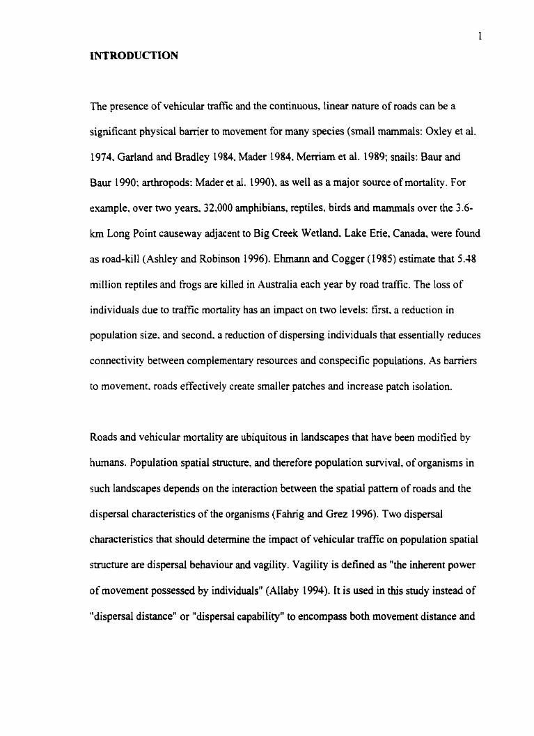
INTRODUCTION

The presence of vehicular t r f i c and the continuous. linear nature of roads can be a

significant physicai banier to movement for many species (smail mammais: Oxiey et al.

1974. Garland and Bradley 1984, Mader 1984. Memam et al. 1989; mails: Baur and

Baur 1990: arthropods: Mader et ai. 1990). as well as a major source of mortality. For

exarnple. over two years. 32.000 amphibians, reptiles. birds and mammals over the 3.6-

km Long Point causeway adjacent to Big Creek Wetland. Lake Erie, Canada, were found

as road-kill (Ashley and Robinson 1996). Ehmann and Cogger (1985) estimate that 5.48

million reptiles and fiogs are killed in Australia each year by road traffic. The loss of

individuals due to traffic mortality has an impact on two levels: first. a reduction in

population size. and second. a reduction of dispersing individuals that essentially reduces

connectivity between cornplementary resources and conspecific populations. As barrien

to movemeni. roads rffectively create smaller patches and increase patch isolation.

Roads and vehicular mortality are ubiquitous in landscapes that have been modified by

humans. Population spatial structure. and therefore population sumival. of organisms in

such landscapes depends on the interaction between the spatial pattern of roads and the

dispersal characteristics of the organisms (Fahrig and Grez 1996). Two dispersai

charactenstics that should determine the impact of vehicular trafic on population spatial

structure are dispersai behaviour and vagility. Vagility is defined as "the inherent power

of rnovement possessed by individuals" (Allaby 1994). It is used in this study instead of

"dispersai distance1' or "dispersai capability" to encompass both movement distance and

fiequency. Dispersal behaviour will determine when, how. and if organisms cross reads.

Vagility will determine the frequency with which organisms encounter roads and incur

vehicular collisions. I expect a more vagile species to be more sensitive to traffic

mortality than a less vagile species for this reason. The optimal dispersal distance for

organisrns that cross roads is then dependent on the distance between habitat patches and

also on the mortality rate incuned during dispersal.

In this study, I evaluated the impact of vehicular traffic on the population abundance of

rwo syrnpatric amphibian species of differing vagility. Rana clamitans (green frog) and

Rana pipiens (leopard frog). Amphibians are well known victims of vehicular mortality

(van Gelder 1973. Fahng et al. 1995) due to the importance of dispersal in anuran

population dynarnics. Breeding popuiations are spatially separated so that the long-

distance dispersal of juvenile tiogs is the major source of gene 80w between populations

( Rittscho f 1975, Breden 1987. Berven and Grudzien I99O). colonizations and

recolonizations of local extinctions (Gill 1978, Sjogren 199 1 ). Rana clamitanr and Ranu

pipiens experience a seasonal shift in habitat that necessitates rnovement between distinct

habitat types in order to fulfill overwintering, reproduction and foraging requirements

(Gilhen 1984). Rana pipiens is considered a more vagile species because it undenakes

three rather than two yearly migrations between habitats. and has longer adult and

juvenile dispersal distances compared to Rana clamitans. As such, Rana pipiens should

encounter roads more often than Rana cfumirans and incur greater trafic mortaiity.

3

1 used population abundance in relation to traffic density in the surrounding landscape to

compare the impact of potential road mortaiity on Runa pipiens (more vagile) and Rana

clamitans (Iess vagile). I hypothesized that vehicular related mortality is sufficient to

significantly negatively impact population abundance and therefore population

penistence of both Rana clamitans and Rana pipiens. However, because Rana pipiens is

a more vagile species, it should experience a greater decline in population abundance in

relation to traf-Tic density than Rana clami!ans (steeper slope in Figure 1).

The goals of this study were to relate population abundance of Rana clarnitans and Rana

pipiens to traffic density in the surrounding landscape and to determine the distance at

which traffic density has the greatest effect on population abundance.

b Traffic density

Figure 1. Hypothesized effects of road traffic density abundance of Rana pipiens and Rana clamitans. Rana pipiens should incur a greater population decline (steeper dope) with increasing traffic density compared to Rana clamitans. Rana pipiens is a more vagile species than Rana clamirans and should incur greater traffic mortality. Initial population sizes are arbitrary .

BACKGROUND

Rana clamitans and Rana pipiens have broadly sympanic ranges (McAlpine and

Dilworth 1 989). Green fiogs range throughour eastern North Amerka (Behler and King

1995) while Leopard fiogs have a greater range which extends across Canada (Giihen

1984), and fiom northem Canada to Panama a range far more extensive that that of any

other North Amencan anuran (Dole 1965). Green and Leopard frogs have been observed

in the Ottawa-Carleton region since 1883 (Mike Oldham- Ontario Herpetofaunal

Summary. personal communication). Where their ranges overlap, they are commonly

found in the sarne breeding ponds (Collins and Wilbur 1979, Hecnar and M'Closkey

1997. blartof 1953a).

Life cycle and movement

Green and leopard fiogs experience a shifl in habitat related to the seasons and distinct

phases of their Iife history. Green frogs occupy two distinct habitats. overwintering and

breeding (Gilhen 1984). Leopard frogs occupy three distinct habitats. ovemintering.

breeding and surnmer feeding (Merrell 1977). While both frogs undergo long-distance

migration between these habitats. once in the habitat they are relatively sedentary (Martof

1953 b. Dole 1965). Overall. leopard frogs cover greater distances in the landscape than

green frogs. This is a combined factor of longer dispersal distances and more movements

between habitat types (Table 1).

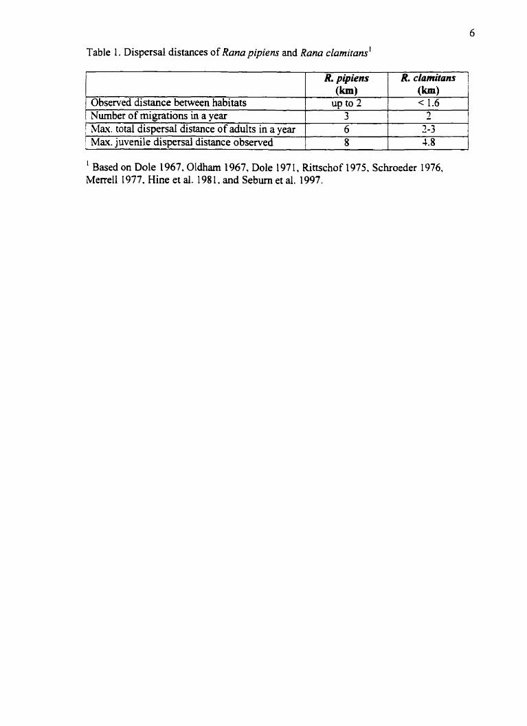
Table 1. Dispersal distances of Rana pipiens and Rona clamitans'

' Based on Dole 1967. Oldham 1967, Dole 197 1, Rittschof 1975. Schroeder 1976. Merrell 1977, Hine et al. 198 1, and Sebuni et al. 1997.

R. clamitans (km) < 1.6

r

Observed distance between habitats

R. pipiens (km)

up to 2 Number of migrations in a year hku. total dispersai distance of adults in a year

3 6

2 - î -3

Max. juvenile dispersal distance observeci 1 8 4.8

7

Adult green frogs have been observed to move 140-640 m during seasonal migration.

between ovemintering and breeding habitat with rnovements probably under 1.6 km

(Oldham 1967). Green frog tadpoles ovexwinter in the breeding pools and transform the

following sumrner at which point they disperse to overwintenng sites. The majority of

observed distances for this dispersal range fiom 184448 m. with rare dispersai events of

2.5 and 1.8 km (Schroeder 1976). In natural populations green Frogs usually reach

maturity in the year following transformation (Wells 1977). Once mature, green frogs are

philopatric to the breeding sites. However, some movement between breeding ponds has

been observed for green frogs either to meet reproductive demands. or to avoid

desiccation (Marto f 1953 b).

For leopard tiogs. breeding ponds should ideaily be within 1.6 km of hbemaculum sites

(Hine et al. 198 1). This finding is sirnilar to that of Merrell(1977) who found that

ovenvintenng. breeding and surnmer habitats were separated by one to two kilorneters.

However. much shorter distances (O-4OOm) between breeding and sumrner habitats have

also been observed (Dole 1967. Hine et al. 198 1). It is possible that an adult leopard frog

may rnove up to 3 to 6 kilometers a year (Merrell 1977). Leopard frog tadpoles transform

at the end of summer (young-o'the-year) and have been noted to move 5-800 rn overland

and 2.1 km downst~eam fiom natal ponds (Dole 1971. Rittschof 1975. Seburn et al.

1997). Leopard fiogs usually mature the second year afier transformation (Hine et

al. 198 1) and have been found in their adult residence, over 1 km (Rittschof 1975). 5.2 km

(Dole 197 1), and 8 km fiom their natal ponds one year later (Seburn et al. 1997).

Habitat

Green Frogs overwinter in the mud and debris in the bottom of swarns about a meter

deep and forage dong the Stream banks before and after breeding (Martof 1953b). During

breeding, green frogs preferentially occupy permanent aquatic habitats with a medium to

high density of emergent and floating aquatic vegetation. muddy and silty bottoms. and

shmbby habitats (Courtois et ai. 1995, McAlpine and Dilworth 1989). Females

preferentially oviposit in dense Elodea mats. other submerged aquatic plants. or sedges in

shallow ( l2.%l4 cm) water near shore (Martof 1956, Wells 1977).

Lropard frogs overwinter in large lakes. spillways below dams at the outlet of lakes.

sueams. and rivers (Merrell and Rodell 1967. Merrell 1977). In the summer. leopard

t iop prefer wet meadows that are close to water and that are not heavily grazed or

mowed (Dole 1967. Merreil 1977. Beauregard and Leclair 1988). Leopards frogs have

bren observed in wet forests during the summer although the extent to which this habitat

type is used is unknown (Dole 1965. Hine et al. 198 1). During breeding, leopard frogs

preferentially occupy temporary or permanent ponds that do not support fish (Merrell

1968). and that have a suong predominance of narrow-leaved and robust emergent

vegetation (Gilbert et al. 1994. Beauregard and Leclair 1988). Egg masses are attached to

herbaceous non-emergent (e.g. Carex) and robust emergent vegetation (e.g. Typha) in

shallow water (65cm) that has been warmed by sunlight (Merreil and Rodell 1967.

Merrell 1977. Hine et al. 198 1, Gilbert et al. 1994).

Methods

Study region

This study was conducted in the Ottawa-Carleton region, Ontario, Canada. The region is

primarily agricultural with forest remnants and some urban settlements. .4gnculture.

roads and urban development have fragmented the terrestrial landscape, while wetland

drainage has reduced aquatic habitat from 45.8 % of the Ottawa area in 1 890 to 1 2.6% in

1982 (Sneil 1987).

Pond seiection

Thirty permanent ponds were surveyed within the Ottawa-Carleton region (Figure 2).

Ponds were spaced at least 1 km apart. to reduce pseudo-replication. Two critena were

used to reduce variation in the data due to landscape composition 1) ponds with similar

landscapes (mostly agriculturd fields) were chosen and. 2) ponds with a low and a high

traffi~c road within 1 km were paired in each area. However. there were more ponds with

low traffic density when trafic density was summed over a 5 km radius. This was due to

the relative paucity of high traffic roads (such as major highways) in the region surveyed.

Ponds had a cleariy defined vegetated edge and were not c o ~ e c t e d to other ponds or

wetlands. resulting in 29 out of 30 ponds k ing man made. New quarries and concrete

pools were excluded as potential sites. Ail ponds were fishless and over 1 0 years of age

except for one that was 6 years old.

Population abundance surveys

Two types of surveys. chorus and visuai, were conducted to increase the accuracy of

determining a relative measure of population size. Chorus surveys count the number of

cailing breeding males, while visuai surveys count the number of frogs (mostly males but

also fernales and juveniles) seen in the breeding ponds.

Chorus swveys

Six chorus surveys were conducted during the peak breeding season of leopard tiogs

between April 17 to May 12. and Four surveys were conducted during the peak breeding

season of green frogs between June 1 to July 3. 1998. The nurnber of s w e y s completed

was detennined as &ce the nurnber of surveys that were necessary to detect presence or

absence. For example. there were no new ponds with calling after three surveys for the

leopard fiog. Therefore six surveys were conducted. Volunteen and rnyself counted the

number of individual calling leopard and green fiog males over a penod of 5 minutes for

each sumey. Three minutes is suficirnt to detect presence and intensity of calling

(Shirose et al. 1997). but not necessarily to count individuals. Where traffic levels were

high. the 5 minutes were the surn of pauses in the background noise (Fahrig et al. 1995).

Volunteers were trained to count anuran breeding calls using the Marsh Monitoring

Program Training audio tape produced by the Canadian Wildlife Service. Inter-observer

agreement of breeding surveys is generally high, although novices tend to underestimate

the nurnber of individuals calling (Shirose et al. 1997).

The ponds were divided into four routes that were dnven in four different sequences ta

vary the beginning tirne of the s w e y for each pond. Routes were driven fonvards.

backward, or starting from a midpoint and moving fonvards or backward (Pope 1996).

Each survey was conducted by a new pair of sweyors to avoid observer bias. Surveys

began 1 /Z h o u after sunset and finished before midnight (Gartshore et al. 1997).

Attempts were made to have ail four routes surveyed on the same night and during nights

of light precipitation (Gartshore et al. 1997), but the use of volunteers made this

impossible. Surveys were initiated for leopard frogs when the air temperature was greater

than 8' (Hine et al. 198 1. Gartshore et al. 1997) and for green frogs when the air

temperature was above 2 1 ' (Gartshore et al. 1997).

Four visual surveys were conducted during the peak breeding season of leopard frogs

between May 5 and 17. and three surveys were conducted during the peak breeding

season of green fiogs between June 1 1 and Iune 26. 1998. Ponds were divided into two

routes that were covered by an assistant and myself during the hours of 9 am and 5 p.m.

over a period of two days. Routes were driven aiternately backwards and forwards to

vary survey times for each pond.

Leopard and green fiogs were counted by the sweyors as they each walked slowly dong

half the waterline, stopping approximately every 2m to scan the waterline. shore and

water ahead (Olsen et al. 1997). Search effort was proportional to the perimeter of the

13

pond and the density of the vegetation. Thick vegetation precluded the scanning method

and required the surveyor to adopt a zigzag pattern so ihat the vegetated area could be

searched adequately. This same pattern was adopted when the shore was tlooded making

ideal conditions for leopard frogs. The entire pond perimeter was surveyed. rxcept for

nvo ponds, where a portion of the penmeter was impassable. Frogs were readily visible

during the day, as Rana spp. are usually found at the waterline. at the water surface. or in

moist vegetation on the shore (Olsen et al. 1997). S w e y s were conducted on sunny calm

days. as cold and windy conditions depress surface activity of many species (Olsen et al.

1997).

Habitat variables

Local pond attributes - pH. perimeter. spawning habitat (m) - and. landscape anributes -

m a of forest. wetland. human development. agriculture fields. waterbodies (km2) and the

lrngrh of streams (km) - were quantified to control for habitat differences in statistical

models (Table 2).

Pond pH

Mean pond pH was based on eight electronic pH rneter readings taken at a depth of jcm.

1 rn out from the shore for the entire pond (Pope 1996). For one pond mean pH was

based on 6 readings. The pH measurements were taken over three days Juiy 30.3 1 and

August 1 1998.

L arxe L v anaules tnciuaea ln xansricar anaiysis

Variable Description

Dependea t

LEOPARD standardized population abundance, which is the sum of the ABUNDANCE visual and chorus survey counts.

GREEN standardized population abundance. which is the sum of the Al3UNDANCE visual and chorus survey counts.

Independent - Local

PH mean pH of pond water LEOPARD OPTIMAL length (m) of optimal spawning habitat LEOPARD SUB- length (m) of sub-optimal spawning habitat OPTIMAL LEOPARD LOW length (m) of low quality spawning habitat GREEN OPTIMAL length (m) of optimal spawning habitat GREEN SUB- length (m) of sub-optimal spawning habitat OPTIMAL GREEN LOW length (m) of low quality spawning habitat

Independent - Lmdscape measured within 1.5 km of the centre of the pond

FOREST area (km') of forested land LETLAND area (km2) of forested and non-forested BLJILT-UP area (km') of human developments including building

complexes. paved areas. residential areas, and cemeteries AGRICULTURE area (km2) of new and old agicultural land WATER area (km2) of waterbodies including lakes. ponds, and rivers STREAM length (km) of streams including ditches

Independent - Traffic

- TRAFFIC cumulative traffic density (traffich') in concentric circles

of 0.25,O.S, 0.75, 1. 1.25, 1.5, 1.75,2.2.5.3, 3.5,4.4.5. 5 km radius, fiom the centre of the ~ o n d

Pond perimeter was paced and related to a measurement in meters for 28 ponds. Two

pond perheters were rneasured using topographie maps and aerial photographs.

Spaw ning habitat

Depending on the size of the pond, 4 to 16 equally spaced line transects that evtended 3

rn perpendicular from the shoreline into the water. were assessed per pond. For each

transect I noted the proportion of the transect length that was covered by each vegetation

type (emergent. submergent. and floating). water depth at 1 rn intervals, distance from

shoreline at which the water depth wu 65 cm.. and insolation. Insolation was rneasured

as the mount of sun received during the day (sun dl day. shaded part of the day. and

shaded al1 day).

Three classes of spawning habitat were derived to cncompass gradation in habitat quality

and to acknowiedge that "low" quality habitat might still constinite suitable habitat. The

total perimeter was multiplied by the proportion of transects with optimal, sub-optimal, or

low spawning habitat (Table 3) so that the point samples were converted into estimates of

the length of each quality of spawning habitat for leopard and green fiogs (Pope 1996).

Table 3. Transect criteria for optimal and subsptimal habitats are marked for combination A and combination B. Low quality spawning habitat is any combination not listed.

Transeci criteria Rana clamitans spawning habitat

Rana pipiens spawning habitat

Sub- optimal

Sub- optimal

Optimal Optimal

Insolation: Full sun

> 1.5 m shailow water (< 65 cm)

> I m of shallow water with narrow-leaved emergent vegetation cover more than: a) 30% b) 5%

> 1 rn of shallow water with submergent and/or tloating vegetation cover more than: a) 309'0

Landrcape variables

I quantified the area of forest open and forested wetland, human developments, new and

old agriculture fields. waterbodies (km'). and the length of streams (km) within a 1.5 km

radius fiom the centre of each pond (Figure 3). Ponds with fiogs are most likely to have

other sources of habitat within 1 - 1.6 km (Pope 1996. Hine et al. 198 1). Measurements

were taken fiom digital Government of Canada 1 50.000 topographic maps ( 1979- 1989)

using the digitizing tèanire in MapInfo Pro (MapInfo Corporation 1997). Forest cover is

îàirly accurately represented on topographic maps (J. Houlahan, personal

communication). To check this and other landcoven. I ground-tnithed the area around

èach pond during the month of August by the noting the land use that could be seen from

the side of the road.

Traffic density

The predictor variable of pnmary interest in this study was trafic density. an index of

potential arnount of road rnortality that combines road density and traffic volume on each

road (Equation 1 ). 1 calculated the cumulative traffic density in concentnc circles

surrounding each pond with increasing radii of 0.25.O.S,O.75. 1, 1 .Z, 1 .S. 1.75.2,Z.j. 5.

3.5.44.5, 5 km (Figure 3). Road length was measured fiom digital Govemment of

Canada 1 50.000 topographic maps ( 1979- 1989) using MapInfo Pro (Maplnfo

corporation 1997). Tdc volume was measured as Average Annual Daily (24h) Traffic

(AADT) counts. AADT counts were supplied by Ottawa-Carleton townships, the

Figure 3. Example of a digital landscape in which the landscape habitat variables and t r a c density wexe measured. Concentric circles of radii 0.25,0.5,0.75, 1 .O, 1.25, 1 5, 1.75,2.0,2.5,3.û, 334.0, 4.5, 5.0 kmare indicated.

19

Regional Municipality of Ottawa-Carleton Transportation department, and the Ontario

Ministry of Transportation Eastern Region TratXc Section. For minor roads that iacked

traffic counts, the township provided an estimate. For residential areas 1 multipiied total

road length by an average AADT count for the residential area. AADT counts for grave1

and residential roads (69% of al1 roads). minor paved roads ( 17%). major paved roads

( 1 I Oh), and highways (jO/a) were, respectively, 0-990, 10004990, 5000-9990. and

10.000- 16000.

Equation 1.

Traffic density ( t raf f ich ' ) = [ ' = " ( I I * .UDT 1 ) ] ACC 1 = l

where n = the total number of roads

I , = length of road,

.L-I DT, = Average Annual Daily T r a c for road,

. K C = Ares of concenvic circle (kmL)

Statistical Xnaiysis

Dependent variable

The abundance counts for each of the visual and chorus surveys were surnrned over al1

sweys (7 and 10 respectively) to give weight to those ponds that had consistent calhg

as well as high calling numben (Pope 1996). This method avoids using a "maximum

count value" that codd be sensitive to differences in clhatic conditions during difXerent

20

survey nights. Population abundance counts fiom the visual and chorus s w e y s were

highly correlated for both leopard frogs (r2= 0.19. p= 0.0 175) and green frogs (r2=0.054.

p=0.001) and were therefore combined. The summed abundance counts were each square

root transformed then standardized (distribution of zero mean and unit variance) so they

would be equaily weighted when added together. The triifl~fomed standardized visual

and chorus counts were added together to produce one abundance measure for each pond

for each of green and leopard frogs.

.Chiel Bu il Jing

In order to determine the influence of traffic drnsity on population abundance of green

and leopard frogs. 1 used stepwise multiple linear regression in SAS (SAS Institue 1996).

The multiple regression proceeded in three sreps. In the first step. al1 local and landscapr

variables were included to produce the most significant habitat model. In the second step.

each traffic density (TRAFFIC) variable (Table 2 ) was substituted consecutively into the

model îiiom step 1 io determine the most significant radius oCTRAFFIC in t e n s of the

partiai F-value. In the third step. al1 two-way TRAFFtC interaction ternis werr included

with the model fiom step 2 in a stepwise multiple regression. Al1 variables were included

in the final modei when their partial F-value was significant at a=0.05.

In al1 analyses. the assumptions of linear regression were checked through visual

examination of residual plots. Residuals were plotted against each of the indepden t

variables. and the predicted values to test for homogeneity

Residual histogram plots were exarnined for nomality.

of variance and independence.

Spariai dependence

Spatial dependence could exist in the data if ponds located close togrther were more

similar in species abundance than ponds farther apart. This couid be due to biotic or

abiotic features that influence more than one pond or if frogs undertook extensive

movements between ponds during breeding. Spatial dependence would indicate that each

pond was not representative of an independent population and there was

psrudoreplication in the data (Legendre and Fortin 1989. Hinch et al. 1994).

1 explored spatial dependence in the data using semivariance. a method rhat mrasures the

degree of similarity between observations separated by varying distances (lags).

Semivariance is the surn of squared differences between al1 possible pairs of points

separated by distance h (Burrough 1995) (Equation 2). Semivariograms plot the

srmivariance against lag distance h, and allow the visualization of the scale of landscape

pattern (Legendre and Fortin 1989. Turner 199 1 ). If the difference between observations

increases over lag distance. then semivariance increases (increasing slope). This increase

continues until the observations are so far apart they becorne unrelated to each other and

the semivariance equals the average variance of al1 the samples, and the slope of the

semivariogram becomes zero (see Figure 5 ) (Gustafson 1998). Least squares regression

22

was used to fit a mode1 to the semivariogram plot and determine the significance of the

slope.

Equation 2

Semivariance at lag h = [ Z ( x . h ) - 2(.r1)l2 i [2 (n) ]

where h = lag

n = nurnber of observations in sample separated by lag h

Z(x) = the value of amibute Z at point x

RESULTS

Surveys

Leopard frogs were absent From four ponds, twelve ponds had no cdling, and five had no

visual records. Green fiogs were present in d l ponds, but two had no cailing and three

had no visual records. ï he presence of juvenile leopard fiogs in the visual surveys couid

have resulted in more ponds with visual records compared to ponds with calling. One of

the ponds lacked optimal or sub-optimal leopard frog spawning habitat although this was

not the case for the other ponds. Leopard fiogs were present in the surveys Born A p d 17

ro June 26, while green frogs were present from May 5 to the last survey date. July 3.

Calling was more active during the appropnate peak breeding season as defined in the

methods section (Table 4).

Models

There was no evidence of a relationship between green fiogs and the presence of

TRAFFIC in the surrounding landscape. Only the length of streams (STREAMS) within

1.5 km of the pond significantly contributed to the observed variation in green fiog

abundance (F 1.30 = 6.787, p= 0.015) (Table 5). On the other hand. leopard fiogs were

significantly negatively affected by the amount of TRAFFIC within a radius of 1.5 km (F

1-30 = 9.680. p= 0.0046) (Table 6). These results supported my hypothesis that the more

vagile species (leopard frog) would

Table 4. Presence and peak counts of Ranapipiem and Rana clamifans population abundance in chorus and visuai surveys of breeding ponds. Ottawa-Carleton 1998.

S pecies

i Rana pipiens

Rana clamitans

Chorus survey Visual survey

Present in survey

April 1 7- June 18 May 5-My 3

Peak counts

Apnl 30- May 12 June 1 -Juiy 3

Present in survey

May Wune26

Peak counts

Mayj - 17

May 5-lune 26 1 June 1 1 - 26

Table 5 . Andysis of variance of best mode1 relating Rana clamitans landscape. and t r a c density variables.

abundance to tocal,

Nurnber of observations = 30 coefficient d.f. type III SS F stat Pr (F)

intercept - 1.359 1

Table 6 . Anaiysis of variance of best model relating Runu pipiem abundance to local. landscape, and t M i c deiisity variables.

Number of observations = 30 coefficient d.f. type III Partial Partial Pr (F)

SS r2 F stat intercept 4.524 1

OPTIMAL (m) TRAFFIC at 1.5 km -5.4 E -05 t 18.238 0.223 9.680 0.0046

(trafEc/ km2)

(traiKc/ km2) * Built-up (km')

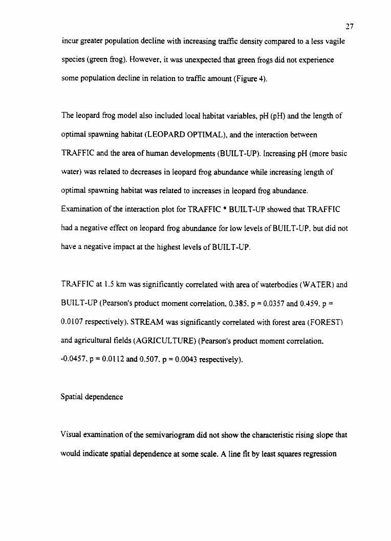
incur greater population decline with increasing traffic density compared to a less vagile

species (green fiog). Kowever, it was unexpected that green fiogs did not expenence

some population decline in relation to traffic amount (Figure 4).

The leopard fiog mode1 also included local habitat variables, pH (pH) and the length of

optimal spawning habitat (LEOPARD OPTIMAL), and the interaction between

TRAFFIC and the area of hurnan developrnents (BUILT-UP). Increasing pH (more basic

water) was related to decreases in leopard frog abundance while increasing length of

optimal spawning habitat was related to increases in leopard fiog abundance.

Examination of the interaction plot for TRAFFIC * BUILT-UP showed that TRAFFIC

had a negative effect on leopard frog abundance for low Ievels of BUILT-UP. but did not

have a negative impact at the highest levels of BUILT-UP.

TR4FFIC at 1.5 km was significantly correlated with area of waterbodies ( WATER) and

BUILT-UP (Pearson's product moment correlation. 0.385. p = 0.0357 and 0.459. p =

0.0 107 respectively). STREAM was significantly correlated with forest area (FOREST)

and agricultural fields (AGRICULTURE) (Pearson's product moment correlation.

-0.0457. p = 0.01 12 and 0.507. p = 0.0043 respectively).

Spatial dependence

Visual examination of the semivariogram did not show the characteristic nsing dope that

would indicate spatial dependence at some scde. A line fit by least squares regression

28

had a slope close to zero for leopard frogs and a decreasing slope for green frogs. This

indicates a lack of evidence for spatial dependence at al1 distance between ponds (Figure

5). The physical implication of this is that the sarnple spacing was too large to resolve

any pattern for species abundance distribution in the landscape.

0 Leopard O Green I

I 35000

Traffic density

Figure 4. Plot showing the decline of Rana pipiens population abundance with increasing tralfic density. There was no significanr relationship between Rana clamitaru population abundance and trafic density. The residuals of green fiog abundance regressed againsr STREAMS and the residuals from leopard frog abundance regressed against pH and LEOPARD OPTIMAL are plotted against trafic density within 1.5 km.

Figure 5. Semivariance plots for Rana pipiem (A) and Rana clamitans (B) showing no evidence of spatial dependence of population abundance for either species. Semivariance of abundance is ploned against distance between ponds (lag).

DISCUSSION

As predicted leopard fiogs (more vagile species) incurred greater population decline with

increasing trafic density than green fiogs (less vagile species). However, it was

unexpected that green frog population abundance did not cxhibit any relationship with

road traffic in the landscape. There are two possibilities for this. One possibility is that

green frogs incurred large amounts of road mortality but the population was able to

overcome the mortality. ho ther possibility is that green fiogs did not incur large

amounts of road mortality because of a low road crossing rate. The first possibility seems

uniikely since green and leopard frogs have similar mean clutch size, 3750 and 4000 eggs

respectively (Hecnar and M'Closkey 1997). and thus similar capabilities of expanding

their population in response to increased mortality. A low road crossing rate could result

if green frogs were indeed less vagile and/or because they bypass roads by moving along

strearns. Interestingly. there are severai reports of high leopard fiog road mortality

(Bovbjerg and Bovbjrrg 1964. Rittschof 1975. Merrell 1977. Ashley and Robinson 1996.

Linck 1998) but only one report of relativeiy low green frog mortality (Ashley and

Robinson 1996). The explanatory strength o f STREAM on green frog abundance might

provide a due to green frog movement. Green frogs feed dong Stream banks (Miutof

1955b) and drainage ditches have been noted as major dispersal routes for green fiogs

(Shroeder 1976). Ditches also piay an important role in gene flow as movement corridors

for the cornrnon frog (Rana temporaria) (Reh and Seitz 1990). Streams bypass roads by

crossing under rather than over roads and could reduce green frog mortality.

TdXc density was measured at several different scales to determine the size of the

landscape unit that had the greatest effect on anuran population abundance. A landscape

unit of 1.5 km for leopard fiogs in diis study implies that the majority of leopard frog

movement occurs within this distance. Since leopard frogs are the most vagiie muran in

Ontario (Hecnar and M'Closkey 1997), a landscape unit of 1.5 km in radius could provide

a guideline for measurine the impact of landscape variables on anuran populations.

Following this reasoning, ponds should have been placed at least 3 km apart to avoid

overlapping landscapes. Ten ponds were less than 3 km apart, and this could have

resulted in some pseudoreplication. However, the possibility of pseudoreplication is

countered by the lack of spatial dependence in the data as measured by the semivariance.

Determining a causal relationship between t r a c density and leopard fiog abundance.

and lrngth of sueams and green frog abundance was not possible since traffic density and

length of streams were correlated with other landscape features. it is not surprising that

rraffic density increased with increasing area of waterbodies and area of human

developments. In the study region, major developments tended to be near large sources of

water and would result in greater road density and traffic volume. The relationship

between the lcngth of streams (includes ditches) and area of forest (negative) and area of

agiculnirai areas (positive) can be explained by the replacement of forests with

agriculture fields in the Ottawa-Carleton region and the subsequent increase of drainage

ditc hes.

Leopard fiogs had a lower incidence than green fiogs in this study, perhaps due to a

greater sensitivity to local pond variables, pH and length of spawning habitat. It has been

s h o w that a lower pH and a greater amount of spawnhg habitat are positively related to

presence or abundance of anurans (Loman 1988, Pope 1996, Vos and Chardon 1998). For

the green frog, however. "practically any body of fiesh water is potential habitat ....

whether small or large. temporary or permanent, and with or without vegetation (Gilhen

1984).

Relative measures (cal1 and visual counts) of amphibian population abundance were used

in place of the more labour intensive mark-and-recapture method of estimating

population abundance. Cal1 counts appear to represent an index of chorus size. whethrr

chorus size retlects population abundance seems to depend on the species (Shirose et al.

1997). The relationship between chorus size and population abundance has not been

rvaluared for Rana clamitans and Rana pipiens. The fact that the visual and chorus

survey counts were highly correlated suggests that an index of population size was

attained in this study.

impact of vehicular traffic on muran populations

Roads are a potential source of dispersal related mortality in al1 anthropogenically

fiagmented landscapes as roads are required for human access. My results provide

evidence that trafic can influence Ieopard fiog population abundance out to at least 1.5

km. This is similar to the Mic-effect distances, 750 m (Vos and Chardon 1998), 1 km

(Findlay and Houlahan 1997). and 2 km (Findlay et al. in press), found in other

amphibian-road studies. The traffic-effect distance is dependent on the movement

distance of the organism and trafic density. Several studies have shown a negative

correlation of survival probability and t r a c volume for crossing amphibians (van

Gelder 1973. Heine 1987, Khun 1987, Fahrig et al. 1995). Estimations of the survial rate

of crossing toads at 2440 cars per hour (624 - 960 AADT) varies from zero (Heine 1987)

to 50% (Khun 1987). At least 30% of roads in this study had AADT values over 600.

Therefore trafic volume should be sufficient to cause large amounts of amphibian

mortality in the Ottawa-Carleton region. Road surveys of migrating amphibians in the

Ottawa-Carleton region found a higher proportion of dead fiogs and toads on hi&-

intensity roads (Fahrig et al. 1995). The differential mortality found by Fahrig et al.

( 1995) suggests that road monality contributed to the observed decrease in population

abundance of leopard fiogs with increased traffic level.

While most fragmentation-arnphibian studies have not taken roads into account (Vos and

Chardon 1998), there is a growing body of studies that have shown a negative correlation

of roads on anuran population pcrsistence. It has been shown that trafic level or density

is negatively correlated with abundance of roadside anuran populations (Fahrig et al.

1995). leopard kog (Ranu pipi en)^ but not green frog (Ranu damitans) populations (this

study). and pond occupation probability of the moor îiog (Rana antalis) (Vos and

Chardon 1998). The number of roads or paved road density has also been shown to be

related to the genetic isolation of the common frog (Rana iemporaria) (Reh and Seitz

1990), herptile species richness in wetlauds (Findlay and Houlahan 1997), and the

35

presence of wood fiogs (Rana sylvarica) and mink fiogs (Rana septen~ionalis) but not

leopard or green frogs (Findlay et ai. in press). The lack of correlation between leopard

frogs and paved road density in the Findlay et ai. (in press) study could be attributed to

the fact that road density was not rneasured beyond 1 km and the response variable was

presence/absence rather than abundance.

Amphibians appear to be vulnerable to the tiagmenting effect of roads and road tratric

(Findlay et al. in press). Terrestrial amphibians are characteristically slow moving and not

cognizant of the danger of trafic (Ashley and Robinson 1996. Vos and Chardon 1998).

Uniike saiarnanders, murans do not appear to avoid roads (deMaynardier and Hunter

1995). Mass migrations result in mass mortality and as Memel1 ( 1977) describes. "At

such tirnes. the slaughter may be so great that the highway becomes slippery because of

the numerous carcasses". Amphibians however. are not the oniy species that have are

vulnerable to road mortality. Vehicular collisions have been recorded for insects.

mammals. reptiles and birds (Forman 1988).

The loss of individuals through traffic mortality impacts leopard fiog populations at both

the local and regional level. At the local level. the population to which the individuals

belong could be reduced in size. At the regiond level, trafic mortaiity is a filtering

process where a proportion of individuals does not successfully cross the road. ï h i s

essentially hgments habitat and reduces landscape comectivity. If killed individuais are

juveniles. then dispersal between populations, recolonizations of local extinctions. and

occupation of new sites could be reduced (Rittschof 1975). Overall, the consequences of

36

trafic mortality are smailer and more isolated populations. Smaller populations are at a

greater risk of e'xtinction by chance, due to demographic, genetic, and envuonmental

stochastic events (Wilcox and Murphy 1985). Isolated populations also have a lower

chance of survivd without the demographic and genetic input of immigrants. and of

recolonization after extinction (Lande 1988).

Amphibian decline

Amphibian populations may be declining worldwide. The cause is presumed to be a

complex mixture of local (agricultural pollution, habitat destruction and fragmentation)

and possibly global (acid min. ultra-violet radiation. climate change) conditions

( Blaustein et al. 1994. Blaustein and Wake 1 995. Pounds and Crump 1 994).

More specifically. the genus Ranidae has experienced population declines through the

L 970s and carly 1980s followed by an increasing trend to the present (based on 89 1

amphibian populations mostly in Western Europe and North America) (Houlahan in

press). This fluctuation codd be attributed to the wide oscillations in population size

characteristic of arnphibians (Pechmann et al. 1991). Lcopard fiog populations have

declined or become locally extinct over most of the fiog's range over the last 20 years in

North Amerka (Beauregard and Leclair 1988, Gilbert et al. 1994). While some

populations in Manitoba, Canada showed recovery in the 80s (Kooaz 1992), the prairie

populations of Ranapipiens in Alberta, Saskatchewan. and Manitoba were classified as

vulnerable in 1998, and the southern mountain populations in British Columbia were

Implications for landscape ecology

Landscape comectivity is a functional measure, integrating landscape structure and the

ability of an organism to move through and between landscape elements (Taylor et al.

1993). A highly vagile species should have a greater ability to move between landscape

clements and thus perceive a fragmented landscape as still functionally comected (With

and Crisr 1995). However. a landscape structure that results in dispersal-related mortality

might alter the ability of an organism to move benveen landscape elements. especially for

a highly vagiie species. This seerns to be the case for amphibians in highly fiagmented

landscapes. where high terrestrial rnonality is one of or the limiting factor in determining

population size rather than the size of the breeding site (Vos and Chardon 1998). In this

study. traffic mortality incurred during overland dispersai seems to be the cause for local

population declines in the vagile species Rana pipiens. Gibbs ( 1998) found a similar

result with amphibians where dispersai ability was inversely related to abundance in

habitat patches that were fragrnented due to habitat loss. Gibbs (1998) postdates that land

between habitats serves as a demographic "draint' for many amphibians and that species

that rely on dispersal are at a disadvantage in landscapes with large amounts of

intervening habitat. Dispersal-related mortality could affect the ability of individuais to

utilize heterogeneous environments and to maintain spatially separated populations (e.g.:

a metapopulation or source-sink dynamics). These populations may lose their advantage

39

and face overall extinction, if individual populations cannot be maintained or recolonized

through dispersai (Opdam 1993).

Leopard and green fiogs both have relatively high dispersal capabilities compared to

other anurans (Hecnar and M'Closkey 1997) yet they reacted very differently to traffic

density in this study. This emphasizes that "dispersal capability" should not be used to

predict how an organisrn would react in a fragmented habitat without a clear

undentanding of its population dynamics. movement pattern and the quality of the

intervening habitat (matrix). A "neutral" matrix. one that does not incur mortality. is a

simpIiQing assumption made in rnany models that regard the effect of dispersal on

species' response to patchy habitats (e.g. With and Christ 1995. Lindenmayer and

Possingham 1996). The presurnption of a neutral matrix is that a vagile species has a

higher tolerance to habitat fragmentation then a less vagile species, a widely held notion

(Gibbs 1998). However. the negative impact of traffic mortality on arnphibian

populations demonstrates that the assumption of a neutral matrix is not valid for some

landscapes or species.

Future research

This study has demonstrated that trac mortality is large enough in the Ottawa-Carleton

region to cause population decline of leopard frogs. The next step is to determine the

mortality rate fiom vehicular collisions (extraneous rnortality) and to relate this to the

base or "naturai" mortdity rate. This relationship could be simulated over a range of

40

extraneous and naturai mortality rates to answer the question. what level of extraneous

mortality will cause population decline? This is an important question for species in

fragrnented habitats where mortality may be higher in the matrix. or dong forest edges

(Murcia 1995). Population demographics other than natural mortality rate also play a role

in the ability of a population to absorb extraneous sources of mortaiity. Demographics.

such as initiai population size and fecundity, shouid be included in the simulation mode1

to determine the impact of extraneous mortality on different species guilds.

Conciusions

Severai conclusions can be drawn from my results. First. disturbance free "buffer zones"

should be or Ieast 1.5 km to protect amphibian populations. Second, a high dispersal

rnonality rate could outweigh the benefits of dispersal in a t'rûgmented landscape. Third.

dispersal-related mortality in roaded landscapes is suficient to cause population level

decline in some species. Fourth, measures of "dispersai capability" should not be used to

predict how an organisrn would react in a fragmented habitat without a clear

understanding of its population dynamics, movernent pattern and the quality of the

matrix. Finaily, transportation and resource officiais should be alerted to the widespread

threat that roads pose to wildlife.

Data- Total c h o u and visual survey counts for each pond

Pond

Bigkidd B imini Burke Cemetery DevereiI Hope Jock

Ranci p @ h s surveys Total chorus

counts

Rona clamitans surveys

4 1 O

2 - 3

O 1 3 O 4 - 7 4

Macgregor Mccauley

b

O'connor Patterson Piilar

Total visual counts

Total chorus counts

O O

O O

Total visual counts

17 O 8 2 7 2 35

5 O 9

9 8

O 8 O

9 3 11

L

3 4 O

L

Rigby Smallkidd s m ~ h

19 25 5 10

O 1

5

2

1 O r

3 44

6 8 7

Pond motel Rec centre Reid

15 O - 7

1

To ta1 Minimum

50 39 2 1 3 1

14 46 9

L O O

23 I L

O 1

13 1 5 10

S pratt Stinson Streit

13 57 26

5 24 7

2 3

2 1

140 O

3 10 O

2 1 O

1

377 1 329 O O

326 O

Data continued- Locai variables

Pond

Bakker (Bell Bigkidd B imini

PH

L

Leopard spawning habitat '

(ml

8 .O4 8 ,O2 9.90 10.30 8 A6

Hope Jock

Optimal

Green spawaing habitat (ml

Burke Cemetery Deverell

Kelly Macgregor Mccauley McNeely blemam jNesbitt O'connor Patterson Pillar Pond motel Rec centre ~ e i d

Optimal'

25 182 20 115 40

8.73 7.92 9.9 1 6.52 8.73

Rigby Smallkidd S myth

Sub- optimal

25 O O

O 84 90

Low Sub- optimal

O 496

O 23 60

18 130

6.67 9.78 10.56 1 1.30 7.20 8.67 7.30 8.48 8.66 8.30 8.16 8.93 6.80 8.71 7.3 3

S pran Stinson Streit Todd Vandam

Mean Minimum Maximum

Low

O O

1 04 O O 16 34 28 62 30 120

O

O 136 49 O O

125 60 30 O 30

125 28 150

50 57 60 72 O

56 32

3 14 114 138 64 17 28 194 30 O 90 O

120 O

6.94 7.90 9.53 8.5 1 8.76

8.50 6.52 1 1.30

56 O

2 1 O 95 69 32 O 28 1 94 60 O

150

42 256 52 19 O 16 68 84 117 30 O

150

1 70 34 O

140 110

25 182

O 69 20

80 57 90 18 O

10 60 42

L

136 68 123 160 110

83 O

3 14

O 1 70 90

42 224 360 38 69 64

68 204 220 20 20

102 34 49 O 20

125 496 20 69 100

1 1

O 64 O O O O

O O O O O

66 O

496

O 60 30 O O

O O

L

119 1 JO 179 30 20 90 40 90 63

30 30 85

40 O

136

108 130

' O O O O

1 O0 O O O 64

O 120

O

O O

67 O

210

111 20

396

11 O

100

Data continueci- Landscape habitat variables

Pond

Bakker Bell B igkidd Bimini Burke

Forest (km2)

1

Cemetery Deverell Hope

0.6 1 3.65 3 .O0 1.8 1 0.96

Water (km')

0.48 2.49 0.8 1

Macgegor Mccaule y McNeel y Merriam Nesbitt O'connor Patterson Piilar Pond motel Reç centre Reid Rigby SmalIkidd Smyth Spratt Stinson S treit

0.08 0.0 1 0.00 0.0 1 0.00

0.10 0.00 0.22 0.0 1 2.72 0.2 1 0.00 0.6 1 1.53 2.66 0.33 0.33 2.56 0.09 0.00 0.00 0.00

Mean Minimum

Built-up (km')

0.57 0.00 0.02

0.06 0.00

1.80 0.43

0.13 0.07 0.00 0.05 0.00

4.03 5.68 3 -34 5.70 2.90 3.13 5.75 3 .O3 3 .O6 3 .O0 2.65 4.04 1.95 4.75 6.45 5 -94 6.25

1

0.03 0.27 0.13 0.4 1 0.00 0.00 0.00 0.02 0.13 0.00 0.22 0.29 0.16 0.15 0.02 0.06 0.00

2.9 1 1.12 3.37 0.44 1.44 3.73 1.3 1 3.4 1 1.39 1 .JO 3.85 2.33 -. 7 41 2.08 0.55 1 .O5 0.73

Wetland (km2)

0.70 0.1 1 0.00

0.00 10.55 1.80 6.69 3.97 2.54 12.86 9.39 5.70 4.73 3 -56 4.60 0.00 4.70 3.8 1 4-95 4.29 '

0.0 1 O .O0 0.00 0.5 1 0.0 1 0.00 0.00 0.00 O .O0 0.0 1 0.02 0.08 0.00 0.00 0.04 0.0 1 0.09

0.13 0.00

0.00

Agriculture (km2)

L

0.42 0.00

Stream (km)

6.25

1.46 ' 3 -93 7.18 '

l

6.36

0.00 0.13 0.00

4.63 t .95

2.69 0.00 7.78 6.49

0.00 0.56 0.03 0.19

5.32 4.3 5 6.23

5 -05 0.00

4.3 1 3.51 5.18 5 -92

44

Data continued- Trafic density variables 0.25- 1.75 km

pond I Radius of concentric circle (km) l

Bell I

B igkidd Bimini

1

1

Burke Cerne tery

Kelly Macgregor Mccauley McNeel y Memam

O'comor Patterson Pi 1 lar Pond motel Rec centre Reid Rigby S mal 1 kidd Smyth S pratt

373 305

9430

219 143

O 7887

59737 872

4325

l I I I

Nesbitt I 17911 29241 35211 39381 42421 47471 51091

588 1003 616

1881 16596

306 O O

1249 8836

319 250

1173 1354 5918

579 167 397

26626 O

6502 O

813 9790 1183

C 1

Mean Minimum

572 343

14800

743 1618 1575

11956 20456

9676 508

261 t 642

Streit Todd Vandam Zane tt i

f 636 14812

772 227 399

36077 80

143 15 O

l 144 14606 1892

3953

2263 533

17895

852 21725 2488

16175 30311

13914 3420 2942 2465

O O

1335 406

348 1 31473

410 346

2186 554

6669

3483 828

20353

1

17138 48 13 6262 4828

01 O

4303 1043

22382 6085

43131

L J

1463 60795 18370 23337 43398

932 34889

3416 18954 35481

886 263 604

41694 1319

18268

9662

7053 52556

L

1031 49817 15168 21401 39025

3983 1834 346 1

62185 2696

25889 768 1 1841

22677 3877

998 46 1

1143 45699

1792 20928

1308 919

1416 4881 1

2165 22931

5349 1613

20543 3186

19663 6082 8548 6679

263

k

1 478 1480 1597

56790 2468

24537 6075 1741

21693 3466

22855 7706

10041 7837

13366

2869' 1323

17366 2563

343

4318 1446

19131 2956

16006 533

19036 21713 828 1043

Data continued- Traffic density variables 2.0-5.0 km

Pond Radius of concennic circle (km) 1 Bakker Bell Bigkidd Bimini Burke C emetery Deverel1 Hope

' ~ e m a m 35452 48370 50789 55029 581 10 60536 62670 Nesbitt 5398 5702 8357 13455 16489 18378 20033 O'comor 4175 505 1 5552 6018 6415 68 15 7172

JO&

Kelly Macgregor Mccauley

2.0 3572 4860 1188

24287 9225

65954 5561 1 29850

Patterson Pillar Pond motel Rec centre Reid

I

71 190 1952

65480 20871

2098 4726

66246 6273

27770 1 1

I 1 1 1 1 1

Maximum 1 800931 865091 932 101 998021 1086881 7595471 764 1 03

3.5 7397 7168 3004

4.0 8497 7959

2.5 4148 5308 t 282

80645 321 1

69478 22766

1

10870 2352

Rigby I

Smallkidd Srnyth S pratt S tinson Streit Todd Vandam

Mean Minimum

3.0 6244 5914 1488

89324 3979

72806 27329

2793 5483

70524 9362

29149

24617 6076

86509 29663 9910

12334

I

23541 43 19

80093 26098 8997

11337

4.5 9679 8760

25998 9824

75074 57536 31685

121492 7630

85297 35282

1

97125 4543

75750 29526

11439 2682

9205' 1977

1

23844 1188

5.0 15754 10342

27744 10334 81737 59171 32973

108688 5080

79693 31715

10146 2219

42127 12101

10631 1 64419 36364

7652 5657

116530 6567

82650 33556

1

12904 3446

1

36033 11697

100976 63350 35558

6842 29463 10843 86896 60966 33926

5647 6834

80145 17075 32452

3642' 5958

73980 10951 30261

27372 15089

107326 38601 12795 14590

25490 10516 93210 32759

1 1 1

32651 11269 93151 62249 34753

43 16 6434

77266 13393 31149

14609 5 470

26166 12807 99802 35504

56397 5470

1

18694 6632

I

58700 6632

26063' 28254

7853 7242

82499 19366 34171

28899 18387

113352 41389 13454 15136

IO854 13189

30382 2682 1282

9320 758 1

84932 30815 35621

29879 22307

117908 45715 14796 15632

12016 13977

32695 3446 1488

REFERENCES

Allaby, M. 1994. Oxford Concise Dictionary of Ecology. Oxford University press: New York.

Ashley, E.P.. and J.T. Robinson. 1996. Road rnortality of amphibians, reptiles and other wildli fe on the Long Point causeway . Lake E ne, Ontario. Canadian Field-Nuiziralist 1 10(3):403412.

Baur. A.. and B. Baur. 1990. Are roads barrien to dispersai in the land snail Ariunta urbustorum'? Canadian Journal of Zoology 68:6 13 -6 1 7.

Beauregard, N., and R. Leclair. 1988. Multivariate analysis of the summer habitat structure of Rana pipiens Schreber (leopard frog) in Lake St. Pierre (Québec, Canada). In Management of .4mmphibians Reptiles. and Srnuif Mummals, pp. 1 29- 143. U.S. Forestry Service General Technical Report RM- 166.

Behler. J.L.. and F. W. King. 1995. A4zrionul A udubon Socieiy Field Guide to Norrh .-fmericnn Reptiles and Amphibians. Alfred A. Knopf: New York.

Blaustein. A.R.. D.B. Wake, W.P. Sousa. 1 994. Amphibian declines: judging stability, persistence. and susceptibility of populations to local and global extinction. Conservafion Biofogy 8( 1 ):60-7 1 .

Blaustein. AR.. and D.B. Wake. 1995. The puzzle of declining arnpbibian populations. Scirnrific American 272(4):52-57.

Berven. K.A.. and TA. Grudzien. 1990. Dispersa1 in the wood frog (Rana sflvarica): implications for genetic population structure. Evolution 22(8):2047-2056.

Bovbjerg, R.V.. and A.M. Bovbjerg. 1964. Swnmer emigration of the frog Rana pipiens in northwestern Iowa. Iowa Acuderny of Science 7 1 :5 1 1-5 18.

Breden. F. 1987. The effect of post-metamophic dispersal on the population genetic structure of fowler's toad, Bufo woodhousei fowleri. Copeia 2386-395.

Bunough, P.A. 1995. Spatial aspects of ecological data. In Daia Analysis in Communify and L a n h p e Ecology, eds. R.H.G. Jongrnan, C.J.R. Ter Braak, and O.F. R. Van Tongeren, pp. 2 13-25 1. Cambridge University Press: New York.

Collins, J.P.. and H.M. Wilbur. 1979. Breeding habits and habiiais ofthe amphibians of' the Edwin S. George Reserve, ~Michigan, with notes on the local distribution offishes. Occasional Papers of the Museum of Zoology No. 686. University of Michigan: Michigan.

COSEWIC. 1999. Canadian Species At Risk. Committtee On the Statu of Endangerend Wildlife In Canada: Canada-

Courtois, D., R. Leclair jr., S. Lacasse, and P. Magnan. 1995. Habitats préférentials d'amphibiens ranidés dans des lacs oligotrophes du Bouclier laurentien, Québec. Canadian Journal of Zoolqy 73 : 1 744- 1 723.

DeMaynardier. P.G., and M.L. Hunter Jr. 1995. The relationship between forest management and amphibian ecology: a review of the North American literature. Ertvironrnental Review 3 230-26 1.

Dole. J.W. 1965. Summer movements of adult leopard fiogs Ranapipiens Schreber. in northem Michigan. Ecology 46(3):Z 6-254.

Dole. J. W. 1967. Spring movements of leopard frogs. Rana pipiens Schreber. in Northem Michigan. The .4 merican hlidland Naturalist 78( 1 ) : 1 67- 1 8 1 .

Dole. J. W. 197 1. Dispersal of recently metarnorphosed leopard fiogs. Rana pipiem. Copeia 2 2 2 1-278.

Ehmann. H.. and H. Cogger. 1985. Australia's endangered herpetofauna: a review of criteria and policies. In Biologv of ..lustralasian Frogs and Reptiles. eds. G. Grigg, R. Shine. and H. Ehmann. pp. 43 -47 . Surrey Beatty & Sons and Royal Zoological Society of New South Wales: Sydney.

F M g . L.. J.H. Pedlar. S.E. Pope. P.D. Talyor. and J.F. Wegner. 1995. Effect of road traftic on amphibian density. Biologieal Conservation 74: 177- 182.

Fahrig, L.. and A. Grez. 1996. Population spatial structure. hurnantaused landscape changes and species survival. Revista Chilena de Historia Nutural69:5- 13.

Findlay. C. S.. and J. Houlahan. 1997. Andiropogenic correlates of species richness in southeastem Ontario wetlands. Conservation Biology 1 1 (4): 1 000- 1 009.

Find1ay.C.S.. J. Lenton. and L. Zheng. Effects of adjacent land use on anuran cornmurtities of southeastem Ontario wetlands. In press.

Foiman, R.T.T. 1998. Roads and their major ecological effects. Annual Review of Ecology and Systematics 29207-3 1.

Garland. T. Jr.. and W. G. Bradley. 1984. Effects of highway on Mojave desert rodent populations. American Midland Natitralist 1 1 1 :47-56.

Gartshore, M.E., M.J. Oldham, R. van der Ham, F.W. Scheuler, C.A. Bishop, and G.C. Barrett. 1997. Arnphibian Road Cd1 Counts Participants Manuai. Ontario Task Force on Declining Amphibian Populations and the Canadian Wildlife SeMce: Ontario.

Gibbs. J.P. 1998. Distribution of woodland amphibians dong a forest fragmentation gradient. Landscape Ecology 13 263-268.

Gilbert. M.. R. Leclair. and R. Fortin. 1994. Reproduction of the northem leopard frog (Runa pipiens) in floodplain habitat in the Richelieu River. P. Québec, Canada. Journal of Herpetolog~ 2 8(4):M35-470.

Gilhen, 1. 1984. Amphibians and reptiles ofNova Scotia. Nova Scotia Musuem: Halifax. Nova Scotia.

Gill. D.E. 1978. The metapopulation ecology of the red-spotted newt. Norophthalmus vir idescens ( Rafinesque). Ecological ~Cfonogruph 48 : 1 45 - 1 66.

Gustafson. E. J. 1998. Quantifying Landscape Spatial Pattern: What is the State of the ilut? Ecosystems 1:143-156.

Hecnar. S.J.. and R.T. M'Closkey. 1997. Patterns of nestedness and species association in a pond-dwelling amphibian fauna. Oikos 80(2): 1 - 1 0.

Heine. G. 1987. Einfache Me& und Rechenrnethode sur Ermittlumg der Überlebenschance wandemder Amphibien beirn Überqueren von Strden. Beih. Fer~;tf' Yaturschuc und Landschafrpflege in Baden- Wïittemberg 4 1 : 473 -9.

Hinch. S.G.. K.M. Somers. and N.C. Collins. 1994 Spatial autocorrelation and assessrnent of habitat-abundance relationships in littoral zone fish. Cunadian Joicrnal of' .-lqirafic Science 5 1 :7O 1-7 12.

Hine. R.L.. B.L. Les. and B.F. Hellmich. 198 1. Leopardfrogpopdutions and mortality in Wisconsin. 1 9 '4-1 976. Techinical bulletin No. 1 22. Department of Natural Resources: Madison. Wisconsin.

Houlahan. J. Temporal. spatial and têronomic trends in 89 1 amphibian populations. In press.

Jackson. S.D.. and C.R Griffin. 1998. Toward a practical strategy for mitigating highway impacts on wiidlife. In Procceedings of the International Conference on Wildlife Ecoiogy and Transportation, eds. G. L. Evink, P. Garret, D. Zeigler. and J. Berry. pp. 17-23. FL- ER-69-98. Florida Department of Transportation: Tallahassee, Florida.

Koonz W. 1992. Amphibians in Manitoba. In Declines N> Canadian Amphibian Populufions: Designing u National Strategy, eds. C.A. Bishop, and K.E. Pettit. pp. 1 9-20. Occasional Paper No. 76. Canadian Wildlife Senice and Environment Canada: Ottawa. Canada.

Kuhn, J. 1987. StraOentod der Erdkr6te (bufo bufo L.): Verlustquoten und Verkehsaufkommen, Verhalten auf der Strai3e. Beih. Veroff Naturschutz und Landschafrpfige in Buden- Württernberg 4 1 : 1 75-86.

Lande. R. 1988. Genetics and demography in biologicai conservation. Science 24 1 : 1455- 1460.

Langton,T.E.S., ed. 1989. rlmphibions and Roads. AC0 Polymer Products Ltd: Shefford, Bedfordshire. UK.

Legendre, P., and M.J. Fonin. 1989. Spatial pattern and ecologicd analysis. C'egerario 80~107-138.

Lindenrnayer. D.B., and H.P. Possingham. 1996. Modeling the inter-relationships between habitat patchiness. dispersa1 capability and metapopulation persistence of the endangered species, Leadbeater's possum. in south-eastern Australia. Landscape Ecology 11(2):79-105.

Linck. M.H. 1998. Reduction in road mortality in a northem leopard frog population. Abstract. A Joint Meeting of the Great Lakes & Central Division Working Groups ofrhe Declining drnphibian Popdations Task Force. Milwaukee Public Museum: Milwaukee. Wisconsin.

Loman. J. 1988. Breeding by Rana remporariu: the importance of pond size and isolation. .Clmuranda Soc. Fauna Flora Fennica 64: 1 1 3 - 1 1 5.

Mader. H.J. 1984. Animal habitat isolation by roads and agriculniral fields. Biological Consenarion 29: 8 1 -96.

Mader. H.J.. C. Schell. and P. Kornacker. 1990. Linear barriers to anhropod movements in the landscape. Biological Conservation 53209-222.

Mapinfo Corporation. 1997. Maplnfo Pro. version 4.5. Mapinfo Corporation. Troy. New York.

Martof. B .S. 1 953 a. Temtonality in the green fiog, Runu clamitans. Ecology 34: 1 65- 1 74.

Martof, B.S. 1953b. Home range and movements of the green fiog, Rana clamitam. Ecology 34(3):529-343.

bIartof. B.S. 1956. Factors influencing size and composition of populations of Rana clamiîons. The American MidIand ivaturaiist 56( 1 ):224-243.

McAlpine. D.F., and T.G. Dilworth. 1989. Microhabitat and prey size among three species of Rana (Anura: Ranidae) sympatric in eastem Canada. Canadian Journal of ZooZogy 67:2214-2252.

Merrell. D.J.. and C.F. Rodell. 1967. Seasonai selection in the leopard fiog, Rana pipiens. Evolurion 2284-288.

Merrell, D.J. 1968. A cornparison of the estimated and the "effective size" of breeding populations of the leopard fiog, Rana pipiens. Evolurion 22(2):274-8 3.

Merreil. D.J. 1977. Life history of the feopard Frog, Rana pipiens. in Minnesota. Occasionai paper No. 15. Bell Museum of Natural History and University of Minnesota: Minnesota.

Memam, G., K. Michal, E. Tsuchiya, and K. Hawley. 1989. Barriers as boudaries for metapopulations and demes of Peromyscus leucopus in farm landscapes. Landscape Ecology 29(4):2?7-23 5.

Murcia C. 1995. Edge effects in fragmented forests: implications for conservation. TREE 1 O(3):58-62.

Oldham. R.S. 1967. Orienting mechanisms of the green fiog. Rana ciamitans. Ecolog -l8(3):477-49 1.

Olsen. D.H.. W.P. Leonard, and R.B. Bury. 1997. Sampling Arnphibians in Lentk Habitats. Northwest Fauna No. 4. Society for Northwestem Vertebrate Biology: Washington.

Opdam. P.. R. Van Apeldoorn. A. Schotman. and J. Kalkhoven. 1993. Population responses to landscape fragmentation. In Landscape ecoiogy ofa slressed cnvironmenr. cds. C.C.Vos and P. Opdam. pp. 147-1 71. Chapman and Hall: London.

Orchard. S.A. 1992. Amphibian population declines in British Columbia. In Declines in Cimadian .-lmphibian Populations: Designing a iVational Strategy. eds. C.A. Bishop and K.E. Pettit. pp. 1 0- 1 3. Occasional Paper No. 76. Canadian Wildlife Service and Environment Canada: Ottawa: Ottawa, Canada.

Oxley. D.J.. M.B. Fenton. and G.R. Carmody. 1974. The effects of roads on populations of srnaIl mammals. Journal of Appied Ecology 1 1 :5 1 -59.

Pechrnann. J.K.. D.E. Scott. R.D. Semlitsch, J.P. Caldwell, L.J. Vitt, and J. W. Gibbons. 1991. Declining arnphibian populations: the problem of separating h m a n impacts from natural fluctuations. Science 253 $92-895.

Pope, S. E. 1996. The relative roles of iandscape complementation und metapopulation dynurnics in the distribution and abundunce of Zeopardfiogs (Rana pipiens) in Ottawa- Carleton. M.Sc. thesis. Carleton University: Ottawa.

Pounds, LA., and M.L. Crump. 1994. Amphibian declines and climate disturbance: the case of the golden toad and the harlequin frog. Conservation Biology 8(1):72-85.

Reh. W., and A. Seitz. 1990. The influence of land use on the genetic structure of populations of the common frog Rana temporuria. Biological Conservation 54239-749.

Rittschof. D. 1975. Some aspects of rhe natural history and ecology of rhe leopardfiog, Rana pipiens. Ph.D. thesis. The University of Michigan: Michigan.

SAS Institute. 1996. SAS user's guide: statistics. Version 6.12. SAS institute Inc., Cary, North Carolina.

Schroeder, E.E. 1976. Dispend and movement of newly transformed green frogs. Rano damitans. The clmeriean ibfidlond Naturulist 95(2):47 1-474.

Sebum. C.N.L.. D.C. Sebum. and C.A. Paskowski. 1997. Northem leopard frog (Rana pipiens) dispersal in relation to habitat. In rlmphibiam in Decline: Canadian Siudies of a Global Problem. ed. D.M. Green. pp.61-72. Herpetologicai Conservation 1. Society for the Study of arnphibians and Reptiles: Missouri.

Shirose. L.J.. C.A. Bishop. D.M. Green. C.J. MacDonald. R.J. Brooks, and N.J. Helferty. 1997. Validation tests of an arnphibian cal1 count survey technique in Ontario. Canada. Herperologica 53(3):3 12-30.

Sjogren. P. 199 1. Extinction and isolation gradients in metapopulations: the case of the pool frog (Runa [essonae). Biological Journal of rhe Linnean Society 42: 135- 147.

Snell. .A. 1987. FVefZand distriburion and conversion in southern Onturio. Working Paper No. 48. Canada Land Use Monitoring Program. Inland Waters and Lands Directorate. Environment Canada: Ottawa, Canada.

Straker. A. 1998. Management of roads as biolinks and habitat zones in Australia. In Proccedings. of rhe International Conference on WiidI#ie Ecology and Transportut ion. eds. G. L. Evink. P. Garret. D. Zeigler, and J. Berry. pp. 1 8 1-88. FL-ER-69-98. Flonda Department of Transportation: Tallahassee, Florida.

Taylor, P.D., L.Fahig, K. Henein, and G. Memam. 1993. Connectivity is a vital element of landscape structure. Oikos 68(3):571-573.

Turner. S.J.. R-V. OWeiil. W. Coniey, M.R. Conley, and H.C. Humphries. 199 1. Pattern and S cale: S tatistics for Landscape Ecology . In Quantitaiive Methods in Landscape Ecologv. eds. MG. Turner and R.H. Gardner, pp. 17-50. Springer-Ver1ag:London.

van Gelder. J.J. 1973. A quantitative approach to the mortality resulting h m baffïc in a population of Bufo bufo L. Oecologia 13 :93-95.

Vos, C.C., and J.P. Chardon. 1998. Effects of habitat fragmentation and road density on the distribution pattern of the moor fiog Rana orvalis. Journal of Applied Ecology 3544- 56.

Wells, K.D. 1977. Temtoriality and male mating success in the greenfrog (Rano ciarnitans). Ecology 58:750-762.

Wilcox, B.A.. and Murphy, D.D. 1985. Conservation strategy: the effects of Fragmentation on extinction. American Nuturulist 125879-887.

With. KA., and T.O. Christ. 1995. Cntical thresholds in species' responses to landscape structure. Ecology 76(8):2246-2459.