Embed Size (px)
Citation preview

} ,'r., i ,.,/
-r """, .r, f; I ;:-:,i-<
."".--~-,... ,: / i
1-1- i '" ,..--
.:rr I~":::;' CIV~L ENGINEERING STUDIES
STRUCTURAL RESEARCH SERIES NO. 125
INVESTIGATION OF RESISTANCE AND BEHAVIOR OF REINFORCED CONCRETE MEMBERS
SUBJECTED TO DYNAMIC LOADING
I
2:,.~ -~:;: =:~: ::' -. _~.; :,"- ~~. -- __ " r; _~ ._.~ -. ._ .''::''-.
~ =- ~ =- -- --:..:., ~ ,- ~~. ~ ~;' :=::; .~.~.~ -::: =s :-:. .~ ~-'-'-"-~,. .. . ."-
-'=~ ~:~~=:::-=:~~ ---- - .-. ------ --. -~- ~~- .=. =~ ·s
.-y-) 1":,.- _ •. _. -- --::: ..
By
A. FELDMAN
and
c. P. SIESS
A TECHNICAL REPORT
to
- -,. - -- ~ -. ,: .--- -- -- - '-' --
THE OFFICE OF THE CHIEf OF ENGlNEERS
DEPARTMENT OF THE ARMY
CONTRACT DA-49-129-ENG-344
AFSWP NO. 929
30 September 1956
UNIVERSITY OF ILLINOIS
URBANA, ILLINOIS


INVESTIGATION OF RESISTANCE AND BEHAVIOR OF
REINFORCED CONCRETE MEMBERS SUBJECTED
TO DYNAMIC LOADING
by
A .. Feldman
and
Co P. Siess
A Technical Report to
THE OFFICE OF THE CHIEF OF ENGITh"'EERS DEPARTMENT OF THE ARMY
Contract DA-49-129-Eng-344 MSWP No. 929
Department of Civil Engineering University of Illinois
30 September 1956


10
II ..
1110
TABLE OF CONTENTS
INTRODUCTION 0
1. Objective
2. statement of Problem
3· Method of Approach
4. Scope 0 0 0 . 0
50 Acknowledgment
60 Notation
EQUIPMENT 1Th1) INSTRUMENTATION
70 Loading Equipment 0 0 0
Pneumatic Loading Unit Pressurizing System Sequence Control Unit
0
Te s t Frame 0 .. 0 0 0 0 •
General Characteristics
80 Measuring Equipment 0 0
Load 0 • 0 0 0
c 0
ii
1
. . .. 1
. . .01
2
6
lO
10
11
15 16 16
17
17 Reaction 0 0 0 • 19 Calibration of Load and Reaction D;ynamometers 20 Deflection 0 0 0 0 0 0 21 Strain 0 0 0 • 0 0 0 0 0 0 0 0 23 . Acceleration 0 24
90 Recording Equipment 0 25
100 Miscellaneous Equipment 0
DESCRIPTION OF TEST SPECIMENS 28
Ma terials . 0 28
12. Attachment of Strain Gages to Reinforcing Steel 29
13· Casting and Curing of Beams 0 30


TESTS OF BEAMS • • • •
140 Beam Preparation 0 .
150 Test Procedure 0 ••
Test Results 0 • •
Computed Capacity ~nd Deflection 0
V. ANALYSIS OF RESPONSE TO IMPULSE LOADING
18. General Considerations e 0 0 e 0 0 •
190 Single-Degree-of-Freedom Analysis
VI"
VII.
20. Problems Solved with ILLIAC
SUMMARY 0 0 0
REFERENCES
APPENDIX A
APPENDIX B
APPENDIX C
TABLES
FIGURES"
DISTRIBUTION
iii
32
32
33
36
40
42
42
43
46
49
51
52
57
62
65
76


Table Noo
1
2
3
4'
5
6
7
8
LIST OF TABLES
Title
Properties of BeamB
Properties of Concrete Mixes
Properties of ReinfC'.rcing Bars
Test Results
Intermediate Quantiti~s in Computation of Moments" and Deflectio2 s
Computed Moments and L;f1ections
Values of Resistance al.d Load Characteristics Used in Analysis
Key to Comparison of IL~.IAC Results
iv
65
66
67
68
70
71
75


LIST OF FIGURES
Figc No. Title
1 60 Kip Pulse Loading Machine 2 Two Views of Trigger and Auxiliary Piston Assembly 3 View of Control Panel of the Pressurizing System 4 Schematic Diagram of Control Panel 5 Oscillogram of Loading Pulse Produced Using Nitrogen 6 Test Set-Up 7 Cross-Section, Gage Arrangement, and Circuits for
Dynamometers NOSe 1 and 2 8 View of Reaction-Measuring Support 9 Cylinder and Gage Arrangement--in Reaction Dynamometers
10 Two Views of Reaction Dynamometer Block in Grips for Applying Tension and Shear
11 Circuit Diagram for Load and Reaction Dynamometers 12 Deflection Gage 13 Deflection Gage Circuit Diagram 14 Sample Strain Bridge Circuits 15 Accelerometer Circuit 16 View of Oscillographs and Timing Device 17 View of Oscilloscopes and Camera 18 View of Main Shaft Tip and Beam Cap 19 View of Miscellaneous Equipment 20 Steel Reinforcement Detail 21 Idealized Stress-Strain Curve for Steel Reinforcement 22 Steps in Fabrication of Reinforcing Cage 23 A Typical Beam Ready for Testing 24 Location of Deflection Gages 25 Strain Gage Location 26 Beam I-a After Failure 27 Beam I-b After Failure 28 Load and Reactions vSo Time, Beam I-a 29 Load vs. Tensile Steel Strain, Beam I-a 30 Load vs. Compressive Steel Strain, Beam I-a 31 Load vs. Concrete Strain, Beam I-a 32 Load and Reactions ys .. Time, Beam I-b 33 Load vs. Tensile Steel Strain, Beam I-b 34 Load vSo Compressive Steel Strain, Beam I-b 35 Load vs .. Concrete Strain, Beam I-b 36 Load VSo Midspan Deflection, Beam I-b 37 Deflection Shape at Various Percentages of Maximum Load,
Beam I-b 38 Nature of Resistance Function and Load Pulse Assumed in
v
39 Single-Degree-of-Freedom ftBalysis Effect of Steel Yield Point on Response~ t = 10 milliseconds
p 40 Effect of Steel Yield Point on Response~ t = 20 milliseconds
p


Figo No.
41 42
43 44
45 46
47 48 49 50 51 52
53 54 55 56 57 58 59 60 61 62 63 64 65 66 67 68 69 70 71 72 73 74 75 76 77 78 79 80 81
82
LIST OF FIGURES
Title
Effect of Steel Yield Point on Response~
Effect of Concrete Strength on Response~
Effect of Concrete Strength on Response~
Effect of Concrete Strength on Response:
Effect of Change in Initial Slope: t p
Effect of Change in Initial Slope: t = P
Effect of Change in Initial Slope: t = P
Effect of Load Duration on Response: Effect of Load Duration on Response~ Effect of Load Duration on Response: Effect of Load Magnitude on Response:
P = P = P =
t P
Effect of Load Magnitude on Response: t p
Effect of Load Magnitude on Response: t p
ILLIAC Problem Nos 0
tl II
iT n tt
II
Vl II II
n f1
It '/!
Vi II n
II it IT
n 11 If
H fI 11
it 11 n
VI n If
ff It U
TI It tI
It fI !I
Ii lV n
it 11 11
It If it
u 11 It
It n n
11 " tf
It II u
1, 2, 3 4, 5, 6 7, 8;J 9 10" ll, 12 13, 14,7 15 16~ 17 18,? 19, 20 21, 22, 23 24 25, 26, 27 28, 29 30 34, 35, 36 40.9 41, 42 43, 44, 45 46, 47 48, 49, 50 51, 52, 53 57, 58,? 59 60, 61, 62 63, 64, 65 69, 70, 71 84, 85, 86 87, 88, 89 93, 94, 95
Assumed Conditions at Yielding
vi
t P
50 milliseconds
t P
t P
10 milliseconds
20 milliseconds
t = 50 milliseconds p
10 milliseconds
20 milliseconds
50 milliseconds
19.2 kips 31.4 kips 51.3 kips = 10 milliseconds
= 20 milliseconds
50 milliseconds
Assumed Distribution b~ Curvat'~e at Yield Moment Relationship Between qi and fs at Maximum Momento Plot of Nominal fs Divided by fy - versus q' Deflection at Maximum Moment versus qi$


Io INTRODUCTION
10 Objective
The ultimate objective of the investigation of which this
project is a part is to obtain by means of tests of reinforced
concrete beams and analyses of these tests information which will
contribute to a better understanding of and a more accurate predic
tion of the strength and behavior of reinforced concrete structures
subjected to dynamic loadingo
The immediate objective of the work carried out under this
contract was limited to the development of equipment for making
dynamic loading tests on reinforced concrete beams and to the rnaL~L~g
of preliminary and exploratory tests and analyseso
20 statement of Problem
The basic problem is the prediction of the reS~s~anCe and
behavior of reinforced concrete structures subjected to dynamic load
ing as a result of air blast due to nuclear weaponso This requires
knowledge concerning the strength and deformation characteristics of
the individual structural members when subjected to dynamic loadingo
The dynamic characteristics of a member in a structure
depend on several different factors, some of which are discussed.
below 0
(a) One set of factors relate to the characteristics of
the loads induced in the individual members as a result of the
- 1 -

2
external loading applied to the structureo One important cbaracter~
istic is the load-time relationship. Moreover, the dynamic behavior
may depend also on the relative amounts of moment, shear J and axial
load induced in the members as well as on the distribution of the
forces along the length of the membero That is, the behavior of a
simple beam subjected to uniform load with a corresponding distribu
tion of moment and shear along the span-may be different than that of
a beam loaded with a concentrated load or of a beam-column connectiono
Static tests have shown a significant difference in the static resist
ance and deformation characteristics of members subjected to such
different loadings (References 1 and 2)0
(b) Another set of factors relate to the characteristics
of the individual members themselves. The variables which must be
considered in this connection are numerous and may have a fairly wide
range 0 Some of those expected to have a significant effect on
either the strength, deformation, or mode of failure of reinforced
concrete beams subjected to dynamic loads are: the properties of
the concrete and steel reinforcement, including strength of concrete J
yield and ultimate strength of steel, and stress-strain characteristics
of steel in the elastic region; and the amount and nature of the
tension, compreSSion, and shear or web reinforcemento
:5 e Method of Approach
Since the number of variables and their ranges are so great~
it seemed evident that any attempt to study their effects by a compre
hensive empirical and experimental investigation would require an

3
inordinately large number of tests and a correspondingly great length
of timeo Furthermore, unless such an investigation were extended to
include simulated service testing of typical structures, there would
still remain a conside"rable uncertainty regarding the application of
the results to the prediction of the behavior of actual structureso
It was believed, therefore, that a purely empirical approach held no
promise and that this problem should be "attacked by more fundamental
studies, aimed at a more complete understanding of the manner in
which a member or structure provides resistance to load and deforma
tion under dynamic loading and the relation of this resistance to
the properties of the members and the materials or to their known
behavior under static loading.
It was proposed, therefore, that the problem be attacked
in stages and that the phenomena investigated and observed in each
stage should be interpreted and understood or explained fully before
proceeding to the next stageo
40 Scope
The scope of the work covered by this report included~
(a) The modifications to the available impulsive-loading
e~uipment necessary to carry out the proposed tests.
(b) The deSign, fabrication, and checking of the addition
al e~uipment needed for the testso
(c) The deSign, fabrication, and testing of a limited
number of beams re~uired for checking the test setup and for develop
ing techniques ..

4
(d) The making of preliminary and exploratory analyses to
predict the effects of changes in some of the most important vari
ables affecting the behavior of beams under dynamic loading 0
The equipment available at the start of this project
consisted of the impulse-loading device, a frame to support it and
absorb the reaction from it, and the components of the pressurizing
system used with ito It was necessary to make a framework of lO-in.
I-beams to transmit the reactions of a beam specimen to the support
ing frameo Also required were a special tip for the loading piston
and matching cap for the beam to transmit the load to the beam.
Supports for the beam specimens were re~uired that would
allow the measurement of the reacticns downward and upward and would
constitute a simple support conditione The supports, therefore, had
to be able to rotate, move horizontally, prevent the beam from
uplifting, while simultaneously measuring the reaction and any tendency
to uplifto Reaction-measuring supports which meet these requirements
have been designed and fabricated and subjected to extensive checking 0
Other new equipment that was required consisted of deflection gages,
a dummy gage box, switch boxes, electric cable, etco
A preliminary test program was designed consisting of beams
with four different cross-sectional characteristicso Five beams of
one type have been cast, of wtrich two have been tested statically.
These tests served to check the operation of the equipment and to
establish the static properties of beams later to be tested dynamicallyo

The ILLIAC, the automatic digital computer at the Univer
sity of Illinois, has been used to solve the problem of the response
of a single-degree-of-freedom (SDF) system of known characteristics
to a given impulsive loado The response has been determined for 104
combinations of beam and load characteristicso
50 Acknowledgment
Work on this project was begun l July 1955 under Contract
DA-49-129-Eng-344 with the Office of the Chief of Engineers, Depart
ment of the Army. This report covers the work completed through
15 July 19560
5
This project was carried out in the Structural Research
Laboratory of the Department of Civil Engineering under the general
direction of No Mo Newmark, Head of the Department of Civil Engineering.
The work on the project was under the direction of Co Po
Siess, Research Professor of Civil Engineering, and was supervised
directly by Ao Feldman, Research Associate in Civil Engineering.
Other personnel actively engaged in the work included No A. Legatos
and 30 La Lett, Research Assistants in Civil Engineering, and W. Eo
McKenzie, Junior Laboratory Mechanic.
The personnel on another project in the Laboratory, desig
nated AF 33(616)-170, are responsible for the design and manufacture
of some of the e~uipment described in this reporto This e~uipment
includes the impulse loading machine and its pressurizing system and
support framework, and the deflection gages and standard resistance
boards for calibrating the deflection traces.

6
60 Notation
The following notation has been used in the report~
a = acceleration of the beam
A = area of tension reinforcement s
Ai = area of compression reinforcement s
b = width of beam
d = distance from top of beam to centroid of tension reinforcement
d! = distance between the centroids of the compres-
E c
f C
fl C
f! cd
f r
fi S
sion and tension reinforcement
= initial static tangent modulus of elasticity of the concrete determined from tests of 6 by l2-ino control cylinders
= initial dynamic tangent modulus of elasticity
modulus of elasticity of the tension reinforcement
= modulus of elasticity of the compression reinforcement
= computed concrete stress at top surface of beam
= static compressive strength of concrete determined from 6 by l2-ino control cylinders
= dynamic compressive strength of concrete
= static modulus of rupture of concrete determined from 6 by 6 by 20-ino control beams
= dynamic modulus of rupture of concrete
= stress in tension reinforcement
= stress in compression reinforcement
= static yield strength of tension reinforcement
= dynamic yield strength of tension reinforcement

ft y
j
L
M
M e
M max
M Y
n
p
p
pI
p max
p y
Q
static yield strength of compression reinforcement (obtained from tests in tension)
; dynamic yield strength of compression reinforcement
; distance between tension force and center of compression of the concrete in compression on the cross-section of a reinforced concrete beam, divided by ~ and equal to (1 - k'/3)
; depth of neutral axis of transformed section for beams reinforced in tension and compression (straight line theory) divided by ~
d t Id length of beam span
mass of beam
equivalent mass concentrated at midspan
maximum bending moment at section of failure in flexure
bending moment at section of subsequent failure corresponding to yielding of tension reinforcement
E IE , static modular ratio s c
E IE d' dynamic modular ratio s c
magni tude of applied load.
A Ibd s
Allbd s
maximum applied load
; load. corresponding to yielding of tension reinforcement
resistance of the beam
;
7

q'
T
w
=
=
f /f' P yd cd
(pf - pi fV )/f' y y C
= (pf - p~fY )/f n s y c
= (pf - p'f i )/f' S yd cd
=
=
=
=
=
=
maximum resistance of beam
beam resistance corresponding to yielding of tension reinforcement
period of natural vibration of beam
decay time of load
duration of load
rise time of load
width of column s-t~ub along longitudinal axis of beam
o = ratio of slope of work-hardening region to slope of elastic region of tension reinforcement stress-strain relation
oY = ratio of slope of work-hardening region to
E o
E~ o
€ Y
slope of elastic region of compression reinforcement stress-strain relation (determined from tension test)
maximum deflection of beam
= beam deflection corresponding to yielding of tension reinforcement
= strain in tension reinforcement at beginning of work-hardening region
= strain in compression reinforcement at begin-. ning of work-hardening region (determined from tension test)
static strain in tension reinforcement corresponding to beginning of yielding
8

= dynamic strain in tension reinforcement corresponding to beginning of yielding
= static strain in compression reinforcement corresponding to beginning of yielding (determined from tensicn test)
= dynamic strain in compression reinforcement corresponding to beginning of yielding
= maximum curvature in beam at yielding of tension reinforcement
9

10
IIo EQUIPME1'T AND INSTRl~TATION
The equipment and instrumentation necessary to apply load
and record the behavior of the test specimen are as important a part
of the test setup as the specimen itselfo That this equipment
should be reliable ~~d consistent in its behavior is a prime necessity
for the success of the test prograIDo That the equipment and instrumen
tation necessary for a dynamic test are infinitely more complicated
than. the equipment for the static testing of comparable specimens
is perhaps not so obvious, but this fact will be attested to in the
following discussiono
The apparatus is designed to apply and record load, and to
record reactions, deflections at five points along the span, accelera
tion at midspan, strains in the tension and compression reinforcement
and in the concrete.~ all as a function of time 0 It is believed that
all of these measurements are necessary for the complete definition
of the behavior of a test specimen l~der dynamic loading and to
provide adequate bases for comparison with tests of similar specimens
under static loadingo
70 Loading Equipment
The description to follow is taken primarily from Reference
The loading device consists of several basic sections: the
pneumatic loading unit which is the basic loading device, the

pressurizing system, the sequence control system for the automatic
control of the loading and ur~oading processes, and the basic test
frame 0
Pneumatic Loading Unit The pneumatic loading unit, a
11
section of which is shown in Figo IJ consists of three functional
systems~ the main loading system, the loading and unloading system,
a.nd the trigger systemo The main loading system consists of the
main cylinder, the storage cylinder, the main piston, and the main
shaft 0 The load is supplied by compressed gas acting on one face
of the main pistono
Before a dynamic test, equal forces are applied to both
faces of the main piston by the introduction of compressed gas into
the chambers on either side of the piston face, and pressures in the
two compartments are adjusted so that no load is applied to the speci
men through the main shafto At a preset time of loading, the gas on
one face of the piston is permitted to escape and the piston is
loaded by the pressure of the remaining' gaso The unloading process
involves the release of the gas which has been acting on the piston
during the loading processQ
The loading and unloading system and the trigger system
act together to control the application and removal of the load by
allowing the escape of gas from the appropriate chamberso The loading
and unloading systems are identical and consist of the slide valve
cylinder, the slide valve, the slide valve rods, and the auxiliary
cylinders and pistonso The slide valve cylinder is essentially an

12
extension of the main cylinder or storage chamber 0 The orifices of
this cylinder are covered by the slide valve which confines the gas
in the chamber 0 The slide valve is connected to the auxiliary lift
system and the trigger assembly by the slide valve rodso The auxi
liary lift system, composed of two cylinders and two pistons for each
slide valve, provides the force re~uired to move the slide valve away
from the orifices at the desired timeso - By using the auxiliary lift
system the force opening the orifice can be controlled independently
of the gas pressure applied to the maLl piston.
When the orifices are closed, the motion of the slide
valve is prevented by the trigger assemblyo This system consists of
the slide valve restraining link assembly, the trigger piston assembly,
the trigger, the solenoid, and the trigger frame. This system is
shown in Figo 2 along with the auxiliary lift assemblyo The slide
valve restraining link assembly is locked into position by the
trigger and the loads from the slide valve rods are transferred
directly to the frameo To start loading or unloading, the solenoid
of the trigger is energized and the trigger releasede The slide
valve restraining link assembly is pushed aside by the trigger
pistons and the slide valve rods are free to move under the force
applied to the auxiliary pistons 0 As the slide valVe clears the
orifices, the loading or unloading process starts and proceeds at a
rate determined by the volume of gas confined in the chamber, the
area of the orifices and the type of gas confined in the chambero
The rate of application of the load is nearly independent of the

13
pressure of the gas confined in the chamber. After a dynamic test
it is necessary to prepare the pneumatic unit for further use by
mo'ving the slide valves back over the orifices. This is accomplished
with a small hydraulic jack acting between the trigger frame and the
ends of the slide valve rodso
Pressurizing System -- The pressurizing system consists of
the bottled gas supply and manifold} th~ control panel} and the neces
sary tubingo The manifold permits gas from any bottle to be directed
to any supply valve on the control boardo It contains pressure reduc
ing valves so that the tubing in the system is not subjected to the
full pressure of the bottled supplyo The board was originally set up
to handle two different gases through four supply valves, but at
present is used only for nitrogen supplied through two of the valveso
Figure 3 is a photograph of the control panel. Figure 4 is a
schematic representation and illustrates the extreme flexibility of
the systemo Gas from any supply line can be directed into any chamber
through the line interlock valves, and future expansion of the system
is provided for by the panel interlock valveso
As an example of the use of the panel in a dynamic test,
with lines 1 and 3 as the supply lines, one starts with all line
bleeder valves open and all other valves closedo One must also take
the precaution that the slide valves are covering the orifices and
that the triggers on the auxiliary systems for moving the slide valves
are seto Pressure gage line valves 1 and 4 are opened so the pressure
in the auxiliary systems will be indicated on gages 1 and 4. Line

14
bleeder valves 1 and 4 are closed, and supply valve 1, line interlock
valve 1-4, and line valves 1 and 4 are opened to bleed pressure into
the auxiliary systems of the amount necessary to operate those
systems, approximately 350 psio If leaks occur, the pressure redUCing
valve on the manifold line to supply valve 1 can be adjusted to main
tain the desired pressure in the auxiliary systemso
Next, line bleeder valves 2 and 3 are closedo Pressure
gage line valves 2 and 3 are opened so the pressure in the loading
chambers will be indicated on gages 2 and 30 Supply valve 3 and panel
interlock valve 2-3 are opened. Now~ line valves 2 and 3 are slowly
opened and continually adjusted so that there is no net force on the
main pistono The test supervisor, monitoring the load with dynamometer
Noo 2, maintains contact with the operator of the control panel by
telephone and directs whether the pressure above or below the piston
has to be increasedo Due to the fact that the main shaft comes off
the bottom face of the piston and the area of the bottom face is
thereby reduced, the pressure required in the bottom chamber to main
tain equilibrium is greater than that required in the top chamber by a
factor of 1.118. However, the face of gage 3 has been re-marked to
indicate a pressure only 00894 times the actual pressure so that if
the indicated pressures on the face of gages 2 and 3 are kept the same
the net force on the piston will be clOSe to zeroo
When the pressure in the top chamber has reached the desired
amount, determined by the desired magnitude of load, line valves 2 and
3 are closedo The test should then be made as soon as possible since
15
temperature variations cause fluctuations in the pressures and
resultant force on the piston 0 In a test, the sequence control unit
first trips the trigger on the bottom auxiliary system allowing the
slide valve rods t.o move and gas escapes from the bottom auxiliary
system and the bottom ma.in chamber, applying loado Gages 3 and 4
now read zeroo The sequence control unit then trips the trigger
on the top auxiliary system and gas esqapes from it and the top main
chamberJ and the load is releasedo Now all gages read zeroo To
bleed the supply lines after the test~ the valve on the gas bottle
being used is closed and panel interlock valves 1 and 3 are opened 0
Bleeder valves 1, 2J 3~ and 4 are also opened so no air will be
trapped or compressed in the system when the slide valves are moved
back over the orifices and the piston is raisedo
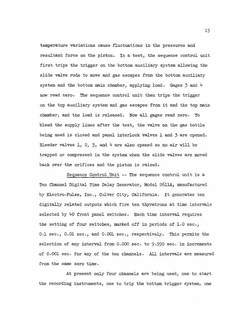
Sequence Control Unit -- The sequence control unit is a
Ten Channel Digital Time Delay Generator j Model 26llA, manufactured
by Electro-Pulse, Inco, Culver City, California 0 It generates ten
digitally related outputs which fire ten thyratrons at time intervals
selected by 40 front panel switcheso Each time interval requires
the setting of four switches p marked off in periods of 100 seco~
Dol secQ, 0001 seco, and 00001 seco J respectively. This permits the
selection of any interval from 00000 seco to 90999 seco in increments
of 00001 seco for any of the ten channelso All intervals are measured
from the same zero timeo
At present only four c:b..ann-els are being usedJ one to start
the recording instruments} one to trip the bottom trigger system, one
16
to trip the top trigger system, and one to stop the instrumentso
Generally, one second may be allowed to elapse between the starting
of the instruments and the tripping of the bottom trigger. The time
between trippings of the triggers depends on the desired duration of
load. Another second may then be allowed to elapse between the time
zero load is reached and the instruments are stoppedo
As an example, if it were desired to apply a load whose
maximum magnitude was to be maintained --for 100 milliseconds, channel 1
would be set for 1.000 seco, channel 2 for 20000 seco, charillel 3 for
2oll0 seco allowing 0.045 sec. for the trigger to act and the load to
rise to maximum magnitude, and cb~nnel 4 for 3.155 seco allowing
0.045 seco for the trigger to act and for the decay of the loado The
unit is accurate to 0.001 sec.
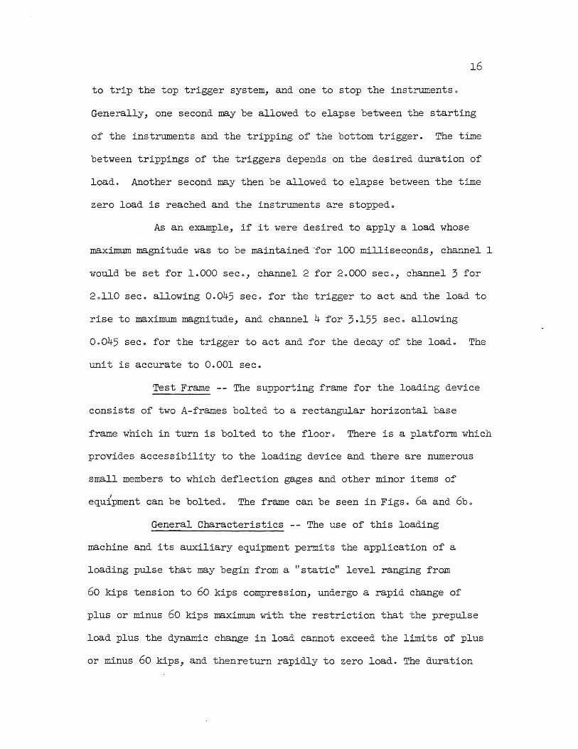
Test Frame -- The supporting frame for the loading device
consists of two A-frames bolted to a rectangular horizontal base
frame which in turn is bolted to the floor 0 There is a platform which
provides accessibility to the loading device and there are numerous
small members to which deflection gages and other minor items of
I
equipment can be boltedo The frame can be seen in Figso 6a and 6bo
General Characteristics -- The use of this loading
machine and its auxiliary equipment permits the application of a
loading pulse that may begin from a "static r1 level ranging from
60 kips tension to 60 kips cOLllllression, undergo a rapid change of
plus or minus 60 kips maximum with the restriction that the prepulse
load plus the dynamic change in load cannot exceed the limits of' plus
or minus 60 kips, and thenreturn rapidly to zero load 0 The duration

17
of the maximum load may be varied from a few milliseconds to many
hours. The loss in compressive loading with the full 18-ino travel
of the piston is approximately 25 per cent of the maximum loado
The rise and decay times of the loading pulse are only
slightly controllable. The minimum time for either rise or decay of
the load is slightly less than 10 milliseconds. It is possible to
change the time re~uired for load application and release using
different gases (helium or nitrogen) in the loading chamberso In
machines of this type, control of the rise and decay times of the
load pulse can be accomplished by changing the areas of the ports on
the slide valve cylinders. However, no provision was made for such
. control on this unito Loads can be applied or released in the rela
tively slow time of two minutes or longer by manual control of the
valves in the pressure supply systemo
Figure 5 is a typical oscillogram of a loading pulse
produced using nitrogen in the main cylinder of the machineo The
period of the timing trace is two milliseconds per cycle and the
magnitude of the peak load is about 35 kips.
8. Measuring Equipment
The various pieces of e~uipment used for measuring load,
reaction, deflection, strain, and acceleration are described below.
Load -- The load applied to the beam specimen is measured
by dynamometers Noo 1 and/or 2. During a calibration test, the reac
tion dynamometers and dynamometer Noo 1 are calibrated against dyna
mometer Noo 2 which has previously been calibrated in a hydraulic

18
testing machine. Dynamometer Noo 2 is read with a static strain
indicator while the signals from Noo 1 and the reaction dynamometers
are recorded on an oscillographo In a static testJ the load is
monitored with Noo 2 to keep the test operator aware of the progress
of the test; however, the load is recorded by Noo 1 on an oscillographo
In a dynamic test, the load is again recorded by Noo 1 on an oscillo
graph while Noo 2 is used to determine the preload on the beam due to
unbalanced pressures in the main chambers of the loading device before
testingo Number 2 can also be used to determine the magnitude of the
peak load if the duration is long enough to permit manual reading of
the indicator connected to Noo 2.
The dynamometers are made of hollow circular steel cylinders
with enlarged threaded ends and are cOPJlected to the threaded main
shaft and to each other by large hexagonal nutso They are visible in
Figo 6ao Dynamometer Noo 2 is placed above Noo 1. Number 1 has
eight SR-4 Type AD-7 strain gages mounted on its outer surface in a
symmetrical alternating patterno Four of the gages are parallel to
the axis of the cylinder and four are circumferentialo The parallel
gages are termed vertical and the circumferential ones horizontalo A
Wheatstone bridge circuit is formed with two horizontal or two vertical
gages in each of the four legs (See Figo 7)0 This arrangement eliminates
the effect of eccentric loading, if present, and multiplies the average
strain output of the vertical legs by approximately 2060 Dynamometer
Noo 2 has four SR-4 Type AD-7 strain gages mounted on its outer surface
in an alternating patterno Two of the gages are parallel to the axis

of the cylinder and two are circumferential. Again, the parallel
gages are termed vertical and the circumferential ones horizontal.
19
A Wheatstone bridge circuit is formed from the four gages with the
vertical gages in opposite legs (See Fig. 7). This arrangement also
eliminates the effect of eccentric loading and results in a signal
output from the bridge equal to 2.6 times the average of the vertical
gages.
Reaction -- The reactions at each end of a beam specimen
are measured in terms of the straL~ in dynamometers built into the
roller support assemblies. The entire assembly is visible in Fig. 8.
These dynamometers each consist of three hollow aluminum cylinders
with enlarged ends firmly attached at each end to 2-in. thick steel
plates. Four SR-4 Type A-7 strain gages are mounted in a symmetrical
pattern on the outside of each cylinder, two parallel to the axis of
the cylinder and two c'ircumferential ~ . The section of the cylinders v.lhere
strains are measured has an outside diameter of 1.3 in. and an inside
diameter 0.9 in. The three cylinders are arranged symmetrically
around the center points of the end plates to which they are attached
(Fig. 9). One Wheatstone bridge circuit is made up from all twelve
gages in each cylinder group. Each leg of the bridge contains a gage
from each cylinder, arranged as shown in Fig. 9 •. This arrangement
eliminates the effect of any eccentricity of load and results in a
signal output from the bridge equal to 2.6 times the average of the
vertical gages. These dynamometer groups have been proof tested
statically under an axial load of 40 kips compression and 20 kips
20
tension and under a compression load of 15 kips wi-~h 005 ina eccentri
city a For each dynamometer, the tension and compression responses are
practically identical and the difference in response under eccentric
loading is negligible.,
Gripping devices were made to permit the dnamometers to
be tested statically in tension and shear simul taneoL31y in the ratio
corresponding to the large end rotations experienced by the beam speci
men in the final stages of a test (See Figo 10) 0 Tt.e shear experienced
by the dynamometers in a test equals the vertical reaction times the
sine of the angle of end rotation of the beam. sincE: the axes of the
dynamometers always remain perpendicular to the longitudinal axis of
the beam., This ar..gle of rotation may be as great as 9 degrees 0 The
results for this test indicate that the difference in response between
the two types of loading, axial tension and combined tension and shearJ
is never more than a strain equivalent to approximately 13C Ibo At
15 kips, the difference is less than one per cent 0
Calibration of Load ~nd Reaction Dynamometers -- In order
to insure that mechanical and electrical conditions during calibration
of the load and reaction dynamometers were the same as during a test,
the following procedure was followed for calibrating these deviceso
Dynamometer Noo 2 was placed in a l20,OOO-lbo capacity Baldwin 'Univers
al Testing Machine and a curve was obtained of axial cc.:rrpressi ve load
vSo strain bridge output as read with an SR-4 indicato}"o All leads
and connections were such that they could be duplicate·i exactly latera
This dynamometer was then attached to the main shaft of the impulse

loading machine and dynamometer No 0 1 was attached below No 0 2. A
steel beam, strong enough to be strained only within its elastic
range under the capacity of the machine, was then placed under the
main shaft and attached dynamometers and supported on the reaction
measuring supportso Load, monitored by dynamometer Noo 2 and read
with an SR-4 indicator, was slowly applied to the beam in distinct
increments by gradually bleeding gas into the loading machineo
Simultaneously, the signals from dynamometer Noo 1 and the reaction
dynamometers were recorded on film by the oscillographs later to be
used in the dynamic testso The wiring between dynamometers and the
recording oscillographs was exactly the same as that used in the
21
beam testso Along with the signals due to actual load, those signals
resulting from placing shunt resistors across a vertical gage leg of
the Wheatstone bridge in each measuring device in turn were also
recorded 0 It was then possible to obtain equivalent load and reaction
values for each of the resistors, later to be used in establishing
the scale of the records obtained during a testo These resistors will
be switched into each circuit to be calibrated and their effect
recorded at the beginning of each testo Any reactive unbalance due
to long leads in any particular bridge was always taken out with a
variable capacitance in the appropriate leg of the bridge before
calibrating or testingo See Figo II for the circuit dia~L-am for the
load and reaction dynamometerso
Deflection -- Deflection of the beam specimens is measured
at five points along the span by slide-wire deflection gageso Fi~~e 12

22
is a drawing of a gage which consists of a piece of nickel-chromium
(nichrome) alloy wire approximately 22 in. long stretched in a steel
frame. The frame is mounted rigidly to the testing machine frame in
such a manner that the wire is in a vertical position. During a test,
the wire is traversed by a slide which is connected to the beam at
mid-height 0 The slide is a piece of steel tubing approximately 22 ino
long with a composition fiber block at one end and a ball and socket
joint at the othero The fiber block contains the sliding contact
which is a thin strip of brass tipped with silvero The ball and
socket joint has a threaded bolt on the ball side of the joint which
is fastened to an aluminum bracket with two nutso The brackets are
made of a T-shaped section, the head of the T being glued to the
side of the beam and the leg having a hole to accommodate the threaded
extension of the slide jointo The slide is guided in its downward
travel by two rods mounted on the gage frame over which the fiber
block fitso Maximum possible travel is 18 in.
Electrical leads come from each deflection gage at three
points; from each end of the wire and from the contacto These leads
go to the deflection resistance boards, which contain a separate set
of calibrating resistances for each gageo The resistances are leD~ths
of the same type of wire as that used in the gagee Knife switches on
the boards serve to introduce greater or lesser lengths of this wire
into the circuit as re~uiredo Figure 13 is the circuit diagram for
the deflection gage systemo
23
It can be seen in Figo 13 that the calibrating resistances
are used to change the relative lengths of two adjacent arms of the
deflection bridges, the other two arms being made of the deflection
gage wire itself as divided by the sliding contacto The lengths of
wire are calibrated in terms of e~uivalent deflection by throwing
the switches one by one and comparing the signal produced on the
oscillograph with that produced by moving the sliding contact on each
gage a predetermined distance. Before a test, those switches for
each gage necessary to give a trace deflection which just encompasses
the range of the expected deflection of that gage are closed and thus
establish the scale of the trace from that gage. It will be noticed
from Figo 13 that one switch for each gage must be closed during a
test or the circuits are incompleteo The switch that is left closed
for a particular gage is the one corresponding to somewhat more than
the greatest expected deflection for that gageo
Strain -- Strains in the tension and compression reinforce
ment are measured with SR-4 Type A-7 gageso Strains in the concrete
on the top surface of the beam are measured with SR-4 Type A-I gageso
Each strain gage is part of an individual Wheatstone bridge circuit
together with three dummy gages of the same typeo For twelve strain
readings, 36 dummy gages are re~uiredo The strain bridge circuits
are very similar to those for the reaction and load dynamometerso
One difference is that there are no condensors in the concrete strain
circuits because the signals from these bridges are recorded on
cathode-ray oscilloscopes utilizing direct current and therefore there
24
is no problem of unbalanced reactance. The circuits for the strain
bridges are shown in Figo 140 The standard calibration resistances
for the strain bridges are the same as those used for the load and
reaction bridges, except that their equivalent values are now
expressed in strain units of microinches per incho These equivalent
values were obtained by shunting the resistors across actual gage
installations on a beam and noting the equivalent strain on an SR-4
indicator. All leads, connections, and switching units were as
nearly as practical the same as those used in a testo As with the
load and reaction bridges, any reactive unbalance due to long leads
is always taken out with a variable capacitance in the appropriate
leg of the bridge before calibrating or testing, except for the
concrete strain bridges as explaLned aboveo Again, these resistors
are switched into each bridge circuit to be calibrated and their
effect recorded at the beginning of each testo
Acceleration Acceleration of the midspan of the beam
under an impulsive load is measured with a Hathaway Type AMS-20A
Electric Accelerometer Head. It can measure accelerations up to
500 go It is mounted on the beam cap during a test and can be seen
in Fig. l8~
A set of calibrating resistances has been prepared for use
with the accelerometero The accelerometer was mounted on a counter
balanced revolving shaft and spun at several different speeds, for
which the corresponding acceleration could be computed, and the
signal output was recorded on an oscillographo calibrating
resistances were then switched in and out of the circuit and the
effect on the signal from the stationary accelerometer recordedo
This provided a measure of the equivalent acceleration of each
resistance for use later in establishing the scale of acceleration
records from a teste The Signal from the accelerometer is one of
changing inductance and must be shifted 90 degrees in phase to be
recorded as changing resistance by an oscillographo Figure 15 is
a schematic drawing of the accelerometer circuito
90 Recording Equipment
The various pieces of equipment used to record the
signals from the measuring devices are described in this sectiono
The Signals from the load, reaction, and steel strain
bridges and from the accelerometer are recorded on film with
Hathaway 8-14 magnetic oscillographs operating with a MRC-18
carrier amplifying system. This system is essentially flat in
response up to 450 cycles per second. The timing trace is marked
25
on the records of these oscillographs with a timing trace generator
employing brass plugs on a rotating disko As the disk rotates, each
plug makes contact with feeler wires, and selected resistances in
the time trace channels of the oscillographs are switched in and out
causing a jump in the trace at regular intervalso
The signals from the deflection gages are recorded with
Hathaway 8-14 OC 2 Group 23 galvanometers, also with a flat response
up to 450 CpSo The time trace is established by the same instrument
as above (See Figo 16)0

26
The signals from the concrete gages are detected on two
DuMont TYPe 333 Dual Beam Cathode-Ray Oscillographs. A mirror device
is used to superimpose the separate images from the two instruments,
mounted one on top of the other, and permits all four traces to be
recorded with one camera, a DuMont Oscillograph-Record camera Type
321-A (See Figo 17)0 The timing signal is generated with a Hewlett-
Packard 200C audio oscillator checked against a Potter Model 830
frequency counter and Z-axis modulation is employed to affect the
brightness of one of the traces periodically and thus establish the
-time intervals. The DuMont camera employs 35 mID. film. After devel-
oping, the record is enlarged before the data is taken offo
There is a gang switch through which the time trace
circuit of the Hathaway equipment and the circuit of a lamp inside
the DuMont camera both passo The light from the camera lamp makes
a continuous mark on the camera film except when the gang switch is
opened 0 This switch, therefore, provides a means of tying together,
with respect to time, the records from the two sets of equipmento
10. Miscellaneous Equipment
Among the various pieces of mechanical and electrical
equipment used on this project are several small pieces which are
indispensable to the smooth performance of a beam test but do not
merit detailed discussiono These include the main shaft tip and
beam cap combination, illustrated in Figo 18, which transmits the
load to the beam and permits the midspan of the beam to rotate
without bending the main loading rod. Also included are the banks

27
of standard resistances, a lOO-point switch box, a dummy gage box
which contains the gages necessary to complete the strain gage
bridge circuits, and aluminum transition boxes which permit the
rapid connection of cables and leads in the various circuitso These
items are illustrated in Figo 19.

28
IIIo DESCRIPrION OF TEST SPECIMENS
The specimens proposed for testing were reinforced concrete
beams 6 by 12 inc in cross-section with a 9-fto span to be loaded at
midspan 0 The beams were cast 10 ft. long with a 6 by 12 in. column
stub at midspan to transmit the loado They were reinforced in
tension, compression, and shearo The cross-section dimensions were
chosen to duplicate those of beams previously tested statically on
another projecto
Five of these beams have been cast of which two have been
tested staticallyo Table 1 contains the values of the percentage of
tension, compression, and shear reinforcement, yield strengths,
concrete strengths and age at testing of the two beams tested with
some of these values for the other three beams that have been casto
Details of the beam configuration, stirrup spacing, and steel arrange
ment are illustrated in Figo 200
II 0 Materials
Information concerning the properties of the materials
constituting a specimen is of prime importance in an experimental
investigation 0 The materials used in this investigation are described
below:
Cement -- Marquette Type 1 Cement was used in all beams.
The cement was purchased in paper bags from a local dealer and stored
under proper conditions.

29
Aggregate -- Wabash Riv~r sand and gravel were used for
all beams. The coarse aggregate had a maximum size of about 1 ino and
a fineness modulus of 605 to 7 and contained a rather high percentage
of fines. The fineness modulus of the sand varied between 300 and 3.2.
Both aggregates passed the usual specification testso The absorption
was about one per cent by weight of the surface-dry aggregateo The
aggregate was purchased from a local dealero
Concrete Mix The mixes used L~ the five beams cast so
far are listed in Table 20 Strengths are reported only for the two
mixes used in the beams that have been tested.
Reinforcing Steel -- All reinforcing steel was intermediate
grade Inland Hi-Bond deformed barso The bars were received in 24-fto
lengths and a 2-ft. coupon was cut from the end of each bar and tested
before the bars were cut and placed in the beams. The bars used in
each beam could thus be matched on the basis of their yield strengthso
The values of the important characteristics for the bars used in the
five beams already cast are listed in the table of reinforcement
properties, Table 3e These quantities are defined in Figo 21.
120 Attachment of Strain Gages to Reinforcing Steel
The first step in the fabrication of a test beam is the
preparation of the reinforcing bars for the attachment of SR-4 strain
gages 0 The location of the gages is determined and the mill scale is
brushed off for a distance of several inches each side of this location.
The lugs on the bar are ground off for a length of about 1-1/2 ino at
each gage locationo The longitudinal rib and parts of the transverse

30
lugs are ground only enough to provide a smooth surface just slightly
wider than the gageo The gages used on the reinforcement are Type A-7
with a gage length of 1/4 ino and an overall width of 5/16 ino The
ground area is then filed and sanded with No 0 120 sandpaper 0 The
gages are mounted and allowed to dryo Drying is accelerated by the
use of infra-red heat lamps. After drying, the gages are covered with
electrical tape and the leads are soldered to them 0 The bars are
then heated and entirely covered L~ the vicinity of the gages with
Petrolastic, an asphaltic waterproofing compound.. This waterproofing
procedure destroys the bond between the steel and the concrete over
a distance of about 2-1/2 in.. at each gage locationo The bars are
immersed in water overnight and the gages are then checked for leakage
resistance 0 Gages with less leakage resistance than 10,000 megohms
are replaced 0 (This, however, is no guarantee against loss of gages
due to mechanical damage during castingc) The bars are then assembled
into a reinforcement cage and placed in the form (See FigG 22)0
130 Casting and Curing of Beams
All beams were cast right side up in a steel form with a
movable side plate to facilitate their removal. The reinforcing cage
was held in position by three chairs made of 1/4-ino mild steel bars.
Two hooks of 1/4-ino mild steel bars were embedded in the top of the
beams near the ends to facilitate handling 0
All concrete was mixed from three to eight minutes in a non
tilting drum-type mixer of 6-cu. fto capacity 0 Each beam was cast
from two batches of concrete of approximately the same proportions.

31
The first batch was placed along the bottom of the beam and the second
batch was evenly distributed over ito Four 6 by 12-ino control
cylinders and one 6 by 20-ino flexure beam were cast from each batcho
The concrete was placed in the forms and cylinder molds with the aid
of a high-frequency internal vibrator.
Several hours after casting, the top surface of the beam
was troweled smooth and all cylinders capped with neat cement pastee
r.~'he beams were removed from the forms the day after they were cast
ard the beams and control cylinders stored under moist conditions for
ar: additional six days. They were then stored in the air of the labor
at(l.~y until tested.
32
IV 0 TESTS OF BEAMS
It was considered desirable to make 2-n initial static test
on a beam similar in properties to the beams to be tested dynamicallyo
Such a test would afford an opportunity to che:.:k all eCluipment and
instrumentation for correct operation at a loading rate slow enough
to permit human detection of faulty behavior a.LJ.d w)uld also provide
a basis for the comparison of behavior under stat~i..c and dynamic condi
tions of loading as well as a comparison with the static tests made
previously (Reference No. 2)0
140 Beam Preparation
The preparation of the beam for testing is the same whe 1 her
the test is to be made dynamically (load duration lO-IOO millisecolds)
or statically (load gradually applied clVer a period of 2 to 3 mir.ltes)o
The beam is marked to indicate the pOEitions of the SR-4 gages for
measilTing concrete strains, the defleetion targets, and the re3.ctions 0
Shortly before the initial set of the concrete occurred7 the top
surface of the beam had been struck smooth ;Jith a finishing trowel.
When this surface is later ground and polished with a porta.ble
grinder;! it is suitable for mounting SR-4 gages.. Only th:.! sro.all area
necessary for the gage is ground 0 A thin layer of' Duco ':.'ement is
applied and allowed to dry before placing the gages.. The gages are
then attached with Duco Cement and light weights are ple.ced on the
felt-covered gages while the cement dries. Heat is not used to
hasten the drying since it could be detrimental to the concreteo To

33
protect the gages, a coating of wax is applied after the cement is
thoroughly dryo The leakage resistance provided with this procedure
is generally greater than 50 megohms.
The deflection brackets are also attached with Duco Cement.
Though the brackets have come loose during a test, there is evidence
that they remained in place until after the max~ resistance of the
beams was exceeded and that it was the jar of the beam hitting bottom
that tore them loose.
After the beam is placed under the piston of the loading
deVice, the reaction measuring supports are moved to the correct
pOSitions under the beam and the beam is lowered and clamped to themo
The slide rods of the deflection gages are then connected to the
deflection brackets and the electrical leads fer the SR-4 gages are
soldered to the gageso Next, all the electrical connections required
for recording and calibrating the various measuring devices are made J
the load transferring cap is placed on the beam, and the beam is
ready for testingo For a dynamic testJ an accelerometer is mounted
on the load transferring capo A beam ready for testing is shown in
Fig~ 230
The location of the strain gages and deflection brackets
for the tests of Beams I-a and I-b are shown in Figso 24 and 25.
150 Test Procedure
up to the point of actually applying the load, the test
procedure used for testing a beam statically is the same as that
which will be used to test beams dynamically~ The zero value of each
measuring device is read with an SR-4 indicator by disconnecting from
the transition box the proper cable leading to the instrument room
and plugging in the indicator in its placeo After the zero readir~s
are taken, all of the cables are replacedo The natural frequency of
vibration of the specimen is determined by hitting the stub vertically
with a sledge hammer and recording the effect on the reaction dynamo
metersc In the future an attempt will be made to record also the
effect on the strain gages and accelerometero Next the main shaft of
the loading device is brought down against the beam and the beam is
again struck with a hammero So far no record has been obtained from
this procedure because of the great amount of damping introduced by
the pistono An attempt will be made to remedy this by increasing the
gain of the amplifiers in the strain bridge circuitso
The calibrating traces for each measuring device are then
put on the records according to the procedures for calibrating
described in the section on equipment and instrumentation 0 The gain
o~ each amplifier is first set so that the calibrating step repre
senting the greatest trace deflection--which in turn represents a
value of strain~ load, acceleration, or deflection greater than that
expected in the test--will remain on the recordo From this point on
the procedures for static and dynamic testing differo
In a static test, the load is monitored with an SR=4 indi=
cat~r connected to dynamometer Noo 2 while gas is gradually bled into
the chamber above the main pistono At several times during the
progress of the test a switch is thrown which simulta~eously marks
all of the recordso For each such mark, the time from the beginning

35
of the test is noted as well as the strain in dynamometer Noo 2 and
the pressure in the loading devicec This procedure ties all of the
records together and provides a check on the load. Once loading
has been started, it is not stopped until the maximum resistance of
the beam has been overcome and its downward travel is stopped by
wooden blocks placed under the midspan of the beam to prevent the
loading piston from travelling too far 0 __ After the beam has hit
bottom, the pressure is bled off the piston and the piston is raised
wi tb a hydraulic jack" The zero value of each measuring device is
read again except for those gages which may have been destroyed in
the testo
In a dynamic test, after the calibration traces have been
put on the records pressure is bled into the auxiliary chambers to
activate the slide valves when the triggers are trippedo Then
pressure is applied to both faces of the loading piston at the same
time, care being taken to keep the forces balanced by monitoring the
procedure with an SR-4 indicator connected to dynamometer No. 20
When the pressure in the top chamber has reached the desired amount,
determined from the area of the piston face (78.54 sqo in.) and the
desired value of maximum load, the inlet valves to the loading
chambers are closedo Next the timing intervals are set on the
sequence control timer and this unit is turned OUo It starts the
records, trips the trigger on the bottom of the loading unit allowing
the gas below the piston to escape and the gas above the piston to
apply the loado After the interval of time preset on the timing unit

36
has elapsed, it trips the top trigger on the loading unit allowing
the gas above the piston to escape and the load drops offo Then the
records are stoppedo
160 Test Results
The results of the static tests of Beams I-a and I-b are
presented in the form of curves, tables, and photographso The photo
graphs in Figo 26 show both sides of Beam I-a after testingo The
cracks were marked with ink for greater contraste Note the buckling
of the compression reinforcement at the edge of the column stub.
Figure 27 shows views of both sides of Beam l-b after testingo Again,
the buckling of the compression steel at the edge of the stub is
apparent 0
When the records of the test of Beam I-a were examined it
was discovered that the load trace went off the oscillograph record
in the direction opposite to that in which dynamometer No.1 had been
calibrated 0 This was due to a mistake in the connection of the leads
from the dynamometer and prompted the writing of a connection instruc
tion sheet to be followed in all subsequent tests. Due to the lack
of a continuous load recordJ the summation of the reactions has been
taken as a measure of the loado Figure 28 is a graph of the summation
of the vertical reactions versus time for Beam l-ao The loading rate
is seen to be quite constant at approximately 13 kips per minuteo To
illustrate the reliability of the reaction values as a measure of
load~ the load determined from dynamometer Noo 2 with an SR-4 indicator
at four stages in the test is plotted as open points on Figo 280
37
The maximum applied load sustained by Beam I-a was 30 kips, in addi
tion to the weight of the beam itselfc
Examination of the records revealed that there was also no
record of deflections because of faulty attachmentof the film magazine
on the oscillograph. Thus it was impossible to plot a load-deflection
curve or strain-deflection curves for Beam l-ac
Figures 29, 30, and 31 are graphs of the summation of the
reactions versus the strain in the tension reinforcement} the compres
sion reinforcement, and the top surface of the concrete, respectively 0
Yielding of the tension reinforcement south of the stub evidently
occurred at a load of 2302 kips and north of the stub at 2302 to 2306
kips 0 The compression steel south of the stub appears to have
sustained some tension at first before being subject to compression,
and yielded at approximately 28 kipso The compression steel north of
the stub yielded at approximately 2404 kipso Gages SO and SP, north
of the stub, were located at the position of maximum sidew'ise buckling
deflection of the compression steel. From Fig. 31, it appears that
crushing of the compression concrete began simultaneously on both Bides
of the stubo After yielding of the steel and crushing of the concrete,
the strain gage signals are rather meaningless, since lead wires were
undoubtedly broken and many gages were completely destroyedo The
gages located in the area of maximum destruction of the concrete were
CA, CB, SA, SB J SO, and SPo
The natural period of vibration of Beam I-a determined as
described in Section 15 was 18 millisecondso

The values of strain at which the gages indicate yielding
took place in the tension steel do not agree with the yield strain
determined from coupon tests of these bars (See Table 3)a This pheno
menon has not yet been satisfactorily explained and may re~uire
extensive checking of the equipment and computationso
Since a complete set of records was not obtained for
Beam I-a, a second beam was tested staticallyo Beam l-b was similar
in all respects to Beam l-a except for a slight difference in concrete
strength; a span reduced by 2 ino from 108 in. to 106 ino, to provide
the end supports with more allowable horizontal movement; and a 2-ino
decrease, from 10 in. to 8 in., in the allowable vertical movement
of the beam at midspane The latter measures were taken to lessen the
chance of jamming of the supports against stops provided to protect
the e~uipment, and were ~uite effectiveo
Figure 32 includes curves of the load as registered by
dynamometer No.1, the reactions, and the sum of the reactions, all
plotted versus timec The open circles are values of load determined
with dynamometer Noo 2 and an SR-4 indicator at three distinct times
during the test~ The discrepancy between the load measured by dyna
mometer No. 1 and either that measured by No. 2 or the sum of the
reactions has been the cause of some concern. Another project in the
laboratory which uses this same equipment has also had some difficulty
with the calibration of dynamometer Noo 1 and steps are being taken
to locate and correct the troublee It is felt that the sum of the
reactions or the values of load determined by dynamometer Noo 2 are

39
more reliable, The sum of the reactions will be used in the remaining
presentation of the results whenever load is indicatedc A loading
rate of approximately 15 kips per minute is indicated by Figo 320
Figure 33 is a graph of load versus strain in the tensile
reiilforcemento There is no curve for gage SA since considerable leak-
age in the gage developed after the beam was cast and its ber~vior
was not consistent~ Yielding of the tension steel on both sides of
the stub appears to have begun at 2205 to 2303 kips~ Gage SD,
farther from the stub than gages SB or se indicates that yielding
reached the section of bar where it was located at a somewhat higher
load j as might be expected 0 Again, the strain at yielding is higher
than that for the coupons cut from the bars later used in Beam I-bo
It is not felt that the rate of straining, approximately 20 x 10-6
inv/ino/sec~, could account for any raised yield strain or delayed
yield phenomena.
Figure 34 is a graph of load versus strain in the compres-
sive reinforcementc Through an oversight at the time of the test,
gages SF and SQ were not calibrated and are therefore not shown in
the figure c: Gage SO, l4 in 0 north of midspanJ appears never to have
received much strainQ Gage SR, 14 ino south of midspan, the side
where greatest damage was suffered, L~dicated yielding at its loca
tion at approximately 28 kips with a corresponding compressive strain
considerably less than the yield strain to be expected for an inter~
mediate grade reinforcing baro Figure 35 is a graph of load versus
concrete strain and indicates that crushing of the concrete occu.rred

40
at approximately 25 kips~ The rate of straining of the concrete
increased sharply at 2303 kips, after yielding of the tensile steel 0
Gage CC, mounted south of the stub, was located at the point of
maximum damage to the beamQ
Figure 36 is a graph of load versus midspan deflectiono
The breaks in the curve at 2300 and 2504 kips correspond to the
development of yielding in the tension reinforcement as detected by
gages SB, se, and SD in Figti 330 The deflection of six inches
corresponds to the maximum load of 2904 kips recorded by the reactionso
Further deflection was recorded by the oscillographs but corresponded
only to the dropping of the beam to the wooden stop at midspano The
deflection configuration of Beam l-b at various percentages of maximum
load is shown in Figo 370 The configurations are nearly symmetrical
but the effect of failure being concentrated south of the stub is
indicated by the higher deflections on that sideo
The natural period of vibration determined as explained in
Section 15 was 18 millisecondso
The results of the tests are tabulated and summarized in
Table 40 Values in Column 7 were computed by multiplying one-half
the average yield load P by 48 ino for Beam I-a and 47 in. for y
Beam I-bo Values in column 8 were computed in the same manner using
p max
17. Computed capacity and Deflection
The computed capacities and deflections of Beams I-a and
I-b are listed in Table 60 The ~uantities in Table 6 were determined

41
from equations and graphs contained in Refo 2. The only departure
from the procedures of Sections 20 and 22 of Refo 2 was the use of
the actual values of E and E 0 Table 5 contains values of the inter-s c
mediate quantities called for in the equations of Refo 20 The assump-
tions, equations, and graphs are reproduced in Appendix A with sample
calculations 0
Columns 5, 6, 7, and 8 of Table 6 contain ratios of the
measured values in the tests to the computed valueso There are no
deflection comparisons for Beam l-a because there were no measured
values 0

42
v 0 ANALYSIS OF RESPONSE TO IMPULSE LOADING
18. General Considerations
The behavior of a reinforced concrete beam under static
loading is generally defined by its load-deflection characteristicso
The behavior of a reinforced concrete beam under impulsive loading is
generally defined by both its resistance-deflection cbaractersitics
and its response, that is, its deflection-time characteristicso As
with static behavior, knowledge of the effect of important variables
on the dynamic behavior is necessary before design procedures for
proportioning members to withstand impulsive loading can be formulatede
In the experimental phase of this program, the load acting on the
beam and the response of the beam will be measured as fu.~ctions of
time. From this information, and measurements of the acceleration
at midspan, the resistance, that is, the resistance-deflection
characteristiCS, can be determined.
A beam subjected to an impulsive lateral load is a vibrat
ing system with an infinite number of degrees of freedom. Its
behavior is further complicated by the fact that there are regions
of both elastic and inelastic action. If the problem could be reduced
to that of a single-degree-of-freedom (SDF) system, the resulting
e~uations and analysis would be much Simpler. An attempt to analyze
the behavior of the test specimens as SDF systems, using correction
factors where necessary to bring the results of analysis in line with
results of tests, is therefore believed to be justifiedo If these
correction factors can be shown to vary in some consistent manner

43
with those variables cr combination of variables which would be kno'\lm
beforehand in a design problem, the analysis as a SDF system is entire-
ly valid. If, however, tID.S is not the case, the analysis as a mul tiple-
degree-of-freedom systen. ma~' be re~uiredo In one instance, that of the
determination of the rea(~tiOlt3 of the beam supports, it is known that
analysis as a SDF system Jielis erroneous results for the initial stages
of response of the simplY-SUPl0rted reinforced concrete beamo Multiple-
degree-of-freedom analysis wil~. almost surely be called for here 0
190 Single-Degree-of -Freedom ill lalysis
The relation govE.rnin S the instantaneous behavior of the
beam under an impulsive loading is
where
Q:::P-Ma
Q = the resistancE of the beam and is assumed to be a function )f t.le deflection only,
P the applied load an~ is a function of time,
a = the acceleration of the beam,
M = the masso
The above relation holds for each :pa.rt.Lcle of the bearno If the
beam is to be considered as a SDF SyStEO, then there must be only
one instantaneous value of Q, M, ane. a lnstead of a multitude
of values. It is most convenient to con~3ider the behavior of the
entire beam in terms of the behavior c,t midspan only, that is,
to consider the acceleration at rnidspa'l as a measure of the accel-
eration of the entire beam, the resistcDce-deflection relation
(1)
44
at midspan as a measure of the resistance-deflec~ion characteristics
of the entire beam, and to consider the mass of the beam concentrated
at midspan. This tlequivalent fl system must res:p:)nd in the same
manner as the midspan of the actual beam iThich is taken to be rep2:'e
sentative of the entire beamo In other vords., the system concentrated
at midspan must exhibit the same behavicr as the midspan of the beam
for which the mass, acceleI"ations, and ':""esis':,ance are distributed
along the entire length of the beamo IJ.)O obtain this corresponden.ce,
the kinetic energy during vibration of the ',Jearn with a uniformly
distributed mass is equated to the ki·:.e tic energy of a beam with an
~J£nown mass concentrated at midspan (Reference 4)0 From this rela
t=~on it can be shown that the mass to be::!oncentrated at midspan is
1/2 the mass of the beam, if it is to be ass~~ed that the shape of
the deflection curve during vibration i::: that of a sine curve;! which
is sufficiently accurate for the ·;last·c range of behavior. The
equivalent mass to be concentrated at midspan is a function of the
assumed deflection shape. If tte deflection curve in the inelastic
range is assumed to be triangular, ~" extreme assumption, then the
mass to be concentrated at mid.8pa.Il ~.3 1/3 the total nass of the beam.
Therefore, it can be expected that ~:.he equivalent mass will vary
d:rring a test from 1/2 to about lls the total mass (See Appendix B)o
Since deflections are 1,eing measured at five points along
the beam, it will be possible to :iraw a deflection curve ,for the
beam at any, time during the test., The equivalent mass to be used in
the analysis of a SDF system ma,' then be determined from energy

considerations. The velocity values needed for this determination
can be assumed either to vary along the length of the beam in the
same fashion as the deflection, or an attempt can be made to compute
velocities as the first derivative of the measured deflection-time
relationships by first differences.
Assuming for the present that the variation of equivalent
mass as a function of midspan deflection has been determined for a
beam, equation 1 can be uniquely solved for the quantity Q, the
resistance, at any given time, utilizing load and acceleration
measurements. The resistance-deflection characteristics of the beam
can then be determined using the resistance-time cp~racteristics as
computed above and the measured deflection-time characteristics 0
The method of determining response described in the previ
ous paragraph requires the multiplication of measured midspan acceler
ation by a computed equivalent mass determined from energy considera
tions in order to obtain the inertia effectso If the assumption of
a SDF system is correct then this procedure is valid 0 If the assump
tion is not correct, then some modified acceleration or equivalent
mass, determined from other criteria, should be used.
Another method for determining the response, which does
not require the use of measured accelerations, is Newmark's ~ Method
which involves successive approximationso It can handle a SDF system
with a changing equivalent mass or a system with several degrees of
freedom. Its use at present on this project is restricted to SDF
systems~ The method requires knowledge of the load and resistance

functions for the mass considered and yields the responseo On this
project, it will be used with assumed resistance functions to give
responses which can be compared with measured responses. The
assumed resistance function which results in the best match of
measured and computed responses can be considered as the resistance
function of the specimen (See Appendix C)o
46
The problem of determining the response of a SDF system
of known resistance characteristics and a constant mass to a given
impulsive load has been coded for the ILLIAC, the electronic digital
computer at the University of Illinoiso The code uses the Newmark ~
Method and re~uires knowledge of the resistance function of the
system, the load pulse, and the period of natural vibration of the
system in the range of elastic behavioro The code re~uires para
meters and yields answers in a dimensiop~ess form; that is, loads in
terms of the yield capacity of the system, deflections in terms of
the yield deflection, and time in terms of the periodo It can handle
resistance and load functions of practically any shape, if they can
be approximated by a series of straight lineso
20. Problems Solved with ILLIAC
A total of 104 problems have been solved on the ILLIAC;
that is, the deflection vSo time response has been determined for 104
combinations of loading conditions and characteristics of a single
degree-of-freedom systemo The nature of the resistance and load
functions assumed in the analysis are illustrated by Figo 380 The

resistance and load characteristics varied in these problems are
listed in Table 7 and are defined below~
~y
Linax P
t r
M e
=
=
=
=
=
=
=
=
yield resistance of the SDF system
maximum resistance of the SDF system
yield deflection of the SDF system
maximum deflection of the SDF system
magnitude of the applied load
rise time of the load
duration of the load
decay time of the load
period of natural vibration of the analogous beam
= mass concentrated at midspan, taken equal to 0.971 lb$-seco 2 per ino for the test beams.
Problems 1 to 30 were intended to represent four differ-
ent beam specimens subjected to various magnitudes and durations of
load with rise and decay times characteristic of those obtained
47
using helium in the loading cylindero Problems 31 to 47 were intend-
ed to represent the first two of the proposed beam specimens,
subjected to the same magnitudes of load as before, but with rise and
decay times characteristic of those obtained using nitrogen in the
loading cylindero Problems 48 to 95 were intended to represent the
first of the proposed beam specimens subjected to one magnitude of

48
load and three different durations but with beam characteristics
computed for various combinations of increased concrete strength
(from 1.1 to 1.6 times the static strength) and increased yield
strength of the reinforcing steel (from 1.1 to 103 times the static
strength). Problems 501 to 509 were intended to represent the first
of the proposed specimens subjected to one magnitude of load and
three different durations but considering the slope of the elastic
part of the resistance curve to be increased up to four times the
slope of the curve computed to represent the static resistanceo
This is equivalent to reducing the' yield deflection by four times.
Of course, the period of vibration is also affectedo
These problems and comparisons between them are plotted
in Figures 39 to 78. The curves at the top in each figure are
assumed resistance curves, the curves in the center are assumed
load pulses, and the curves at the bottom are the responses as
computed on the ILLIAC. Figures 39 to 53 are comparisons of problems
illustrating the effect on the response of variation in particular
quantities 0 Figures 54 to 78 are the problems not included in the
comparisonse Table 8 contains information concerning the compari
sons made in Figs 0 39 through 53.
With information of this type the task of chOOSing a
resistance function to yield a given response and of relating the
chosen resistance function to changes in the properties of' the beam
materials due to high strain rates should be materially eased.

VIo S~Y
The primary objectives of the work described in this report
were: to adapt the available equipment and manufacture the additional
equipment necessary to carry out the proposed tests; to check the
operation of the equipment as individual units and as a unified whole;
to develop testing techniques through the testing of pilot beams; and
to make analyses of various single-degree-of-freedom systems under
different loading pulses to obtain information which will be of value
in the interpretation of future testso
Among the additional equipment fabricated were reaction
measuring supports which simulate simple support conditions while
permitting the measurement of uplift as well as downward reactiono
static tests were made on two beam specimens and provided an adequate
evaluation of the behavior and reliability of the loading, measuring,
and recording equipmento A total of 104 problems have been solved on
the ILLIAC and provide a guide to the selection of resistance func-
tions to match response c~ves obtained from future testso
The mechanical features and operation of the equipment and
instrumentation have been described in detail and illustrated with
figures and photographs. The manufacture of specimens and the proce-
dures for testing them are outlined 0 The results of the two static
tests presented in both tabular and graphical form~ Comparisons
are made between the test results and computed results based on an
existing theory. The solutions to the problems of the response of a

50
single-degree-of-freedom system to an impulsive load are presented
with sample comparisons between problems to illustrate the effect of
certain variables on the response.

VIIo REFERENCES
lo nAn Investigation of the Load-Deformation Characteristics of Reinforced Concrete Beams Up To the Point of Failure, U by Jo Ro Gaston, Co Po Siess, and No Mo Newmark, Civil Engineering Studies, structural Research Series Noo 40, University of Illinois, Urbana, December 1952.
2. ftLoad-Deformation Characteristics of Simulated Beam-Column Connections in Reinforced Concrete/' by Ho Mo McCollister, C. Po Siess, and No Mo Newmark, Civil Engineering Studies, Structural Research Series No. 76, University of Illinois, Urbana, June 19540
3. Eighth Interim Report, Contract Noo AF 33(6l6)-l70, by Fo L. Howland, et al, Urbana, Illinois, June 19550
40 UVibration Problems in Engineering,ft by S. Timoshenko, Do Van Nostrand Coo, New York, New York, Third Edition, January 1955, pp. 26-270
50 ttCornputation of Dynamic Structural Response in the Range Approaching Failure, It by NoM. Newmark, Proceedings of the Symposium on Earthquake and Blast Effects on Structures, Los Angeles, california, June 19520
51

APPENDIX A
DERIVATION OF EXPRESSIONS FOR CRITICAL MOMENTS AND DEFORMATIONS FOR STATICALLY LOADED BEAMS
52
This material is taken primarily from References 1 and 2.
The following assumptions are made in the calculations
for theoretical moment-carrying capacities and corresponding deform-
ations for reinforced concrete beams under static load:
(1) Linear strain distribution. Linear distribution of
strains throughout the depth of the beam is assumed
at all stages.
(2) stress-strain relationship for reinforcemento The
stress-strain relationship for the reinforcement is
assumed to be known. In the calculations, the actual
stress-strain curve of the steel is approximated by
an idealized curve consisting of three straight lines
as shown in Figo 210
(3) No tension resisted by concreteo Tension stresses in
the concrete are neglectedo Although some tension
stresses must always eXist, their effect on the moment-
carrying capacities and deformations of interest in
this report can be neglected with little erroro
(4) Bond between concrete and steel. The bond condition
between the reinforcement and the concrete influences
the condition of compatibility of strainso Perfect
bond is assumed to exist between the concrete and steelo

53
This assumption is not strictly correct since
local bond failures occur in the vicinity of
cracks.
Yield Moment
Figure 79 (Figo 36 of Ref. 2) illustrates the conditions
of strain and stress assumed to exist at yielding of the tension rein-
forcemento
From consideration of the distribution of stresses, taking
moments about the tension reinforcement j
(1)
where
k' = I/{ np + (l-k" )(n-l)p' ] + [(n-l)p' + np ] 2 ~ [(n-l)p' + np ]
From statics,
and from geometry,
where
Yield Deflection
f c
ft s
pf y
n = E IE s c
(2)
(3)
(4)
The curvature is equal to the strain in the tension steel
divided by the distance from the centroid of the tension steel to
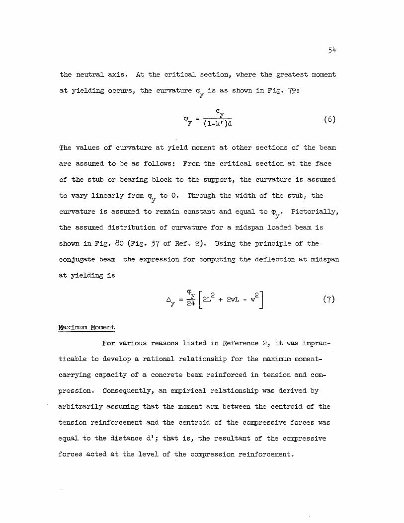
54
the neutral axis. At the critical section, where the greatest moment
at yielding occurs, the curvature ~ is as shown in Fig. 79: y
CPy = €
Y (l-k' )d
(6)
The values of curvature at yield moment at other sections of the beam
are assumed to be as follows: From the critical section at the face
of the stub or bearing block to the support, the curvature is assumed
to vary linearly from ~ to 00 Through the width of the stub, the y
curvature is assumed to remain constant and equal to ~ 0 Pictorially, y
the assumed distribution of curvature for a midspan loaded beam is
shown in Fig. 80 (Fig. 37 of Refo 2)0 Using the principle of the
conjugate beam the expression for computing the deflection at midspan
at yielding is
cp [ 2 2J D.y = ~ 2L + 2wL - w
Maximum Moment
For various reasons listed in Reference 2, it was imprac-
ticable to develop a rational relationship for the maximum moment-
carrying capacity of a concrete beam reinforced in tension and COID-
pression. Consequently, an empirical relationship was derived by
arbitrarily assuming that the moment arm between the centroid of the
tension reinforcement and the centroid of the compressive forces was
equal to the distance d t; that is, the resultant of the compressive
forces acted at the level of the compression reinforcemento
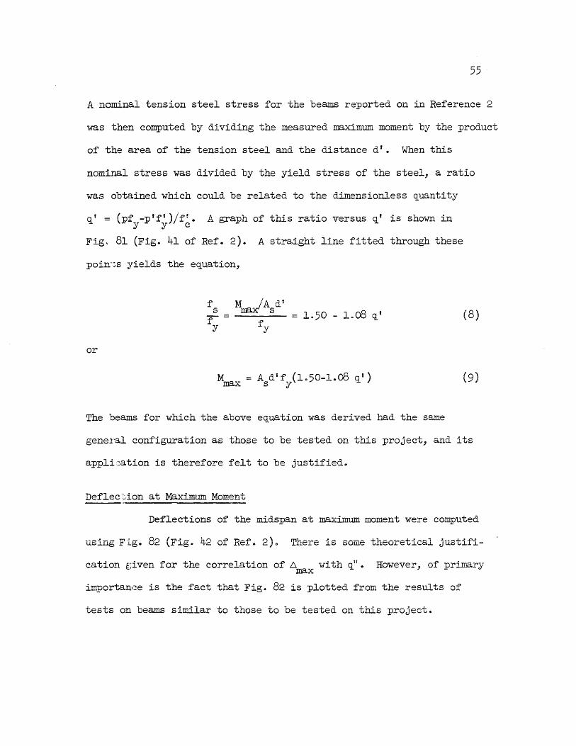
55
A nominal tension steel stress for the beams reported on in Reference 2
was then computed by dividing the measured maximum moment by the product
of the area of the tension steel and the distance d'. When this
nominal stress was divided by the yield stress of the steel, a ratio
was obtained which could be related to the dimensionless ~uantity
~f = (pf -ptf')/f'. A graph of this ratio versus q' is shown in y y c
Fig. 81 (Fig. 41 of Ref. 2). A straighy line fitted through these
poin"-;s yields the equation,
f s M fA d t
max' s
or
r= y
Mmax
fy
The beams for which the above equation was derived had the same
(8)
general configuration as those to be tested on this project, and its
appli:ation is therefore felt to be justified~
Deflec ;::,ion at Maximum Moment
Deflections of the midspan at maximum moment were computed
using Fig. 82 (Fig. 42 of Ref. 2)0 There is some theoretical justifi-
cation [,iven for the correlation of 6 with qUo However, of primary max
importan(!e is the fact that Fig. 82 is plotted from the results of
tests on beams similar to those to be tested on this project.

Sample Computa tion
Fer Beam 1-a, p = 0.0200, p' = 0.0146, ~t
fyom which k' = 0.394 by equation 2.
Now, f = 46.17 kSi, from which f = 3360 psi and f' = 17.96 ksi by yes e(luations 3 and 4, respectively.
r inally, b = 6 in., d = 10 in., A' = 0.88 sq. in., and d t = 8.5 in .. S
from which, by equation 1,
Now € = 000014 in. / in. , from which, by equation 6, cp = O. 00023l/ in 0 y y
Next L = loB in., and w :;;;: 12 in.,
so, by equation 7,
6 = 0.25 in" y
Using f~ = 46.93 ksi, and f~ = 6240 pSi, we obtain 90 1 = 000382
and, by equation 9,
Also, we obtain from equation 8, f = 67035 ksi S
and then q" = 0.106
(See formula in Table 5)
Usir~ Fig. 82, we find
M == 687 in .. ,kips max -------'''--

APPENDIX B
DETERMINATION OF EQUDI ALENT MASS FOR SINGLE-DEGREE-OF-FREEDOM ANALYSIS
This material is taken primarily from Reference 40
57
Consider the case of vibration of a beam of uniform cross-
section loaded by weight P at midspano
I
T L/2 J
If the weight pL of the beam is small in comparison with the weight P,
it can be assumed with sufficient accuracy that the deflection curve
of the beam during elastic free vibration has the same shape as the
static deflection curve for a midspan loaded beam. Then, denoting
by 6 the displacement of the midsp~n during vibration, the displacec
ment of any element pdn of the beam, distant n from the support,
will be
(1)
for 0 < n < L/2
Denoting 6 as the velocity at midspan, and 6 as the velocity of the c n
element pdn, then
6 == n 3nL2 _ 4 3 0
n 6 L3 c
(2)

The kinetic energy of the beam itself will be,
L/2.. L/2 2.3 ., = 2J ~ m(6o )2 dn = 2J ~ R (3nL -4n 6)2 dn
2 n 2 g L.3 c o 0
(.3 )
where g is the acceleration of gravityo
This kinetic energy of the vibrating beam must be added to & 2
the energy P(6o ) /2g of the load concentrated at the middle to obtain c
the total kinetic energy ..
(4)
This formula was obtained for the assumption that the weight
of the beam is small in comparison with the weight Po Even in the
extreme case where P = 0 and where the assumption is made that (17/.35)pL
is concentrated at midspan the accuracy of this concentrating procedure
is sufficiently closeo The static deflection at midspan of the beam
under the action of the equivalent load (17/.35)pL applied at midspan is,
Substituting this into the well-known equation for the period of
natural vibration
T = 2n j 6st:tiC (6)

59
we obtain for the period of the beam with ~~ of the mass concentrated
at midspan,
The exact solution for the fundamental period of a beam on simple
supports with its mass distributed is
(8)
(See Article 52, Reference 4)0
If it had been assumed that the deflection curve of the
beam during elastic vibration was a sine wave, the equivalent mass
to be concentrated at midspan would be 1/2 the total mass of the beamJ
and the computation for period yields the exact value in equation 8
for P = O.
Again, if the deflection cur-~e during elastic vibration
is assumed to be triangular, then the equivalent mass to be concentrat-
ed at midspan is 1/3 the total mass of the beamo Since this deflected
shape would only occur during the inelastic range of behavior, it is
meanir~ess to compute an elastic period of vibration corresponding to
it.
In order to compute the equi~~lent concentrated mass for
some deflected shape which may be measured during the test of a beam,
the following procedure may be used~

60
Given a beam divided into the segments of mass ~, m2,
m , each with a deflection at some given time during vibration n
of~, ~, . !:::. , respectively 0
n
Using the notation!:::. to denote the first derivative of
displacement with respect to time, the velocity of the various masses . .
are ~, 62
, 0 • • 0 6 n, respectively, and their various kinetic energies
are
o
K E = ~ m (!:::.on)2 (~c)2 • on 2 n 6
c W
where!:::. is the velocity at midspano The total kinetic energy of the c
beam is then
n
I 1
m n
(10)
The kinetic energy of an equivalent mass concentrated at midspan is
(ll)
By equating the expressions for kinetic energy we obtain
(12)
To obtaL~ the velocity values needed in equation 12 it may
be necessary to differentiate grapbically the measured deflection-
time curve for each mass of the beam considered. It can be assumed

61
that ~ /~ = 6 /6 ; that is, that the velocity varies along the beam .n c n c
as the deflection. This is strictly true for the cases computed
above for predetermined deflection configurations (sine wave, triangle,
etc.), where the shape of the deflection curve is constant throughout
the cycle of vibration though the magnitude of deflection changes.
However, when the shape as well as the magnitude of deflection changes,
then the velocities no longer vary as the deflectiono This is the
case for a reinforced concrete beam subjected to impulse loading 0 To
assume, therefore, that ~ /6 = 6 /6 is definitely an approximation. n c n c
E~uation 12 can be evaluated at each time increment in a
test from the measured deflected shapes at those timeso Then, a
curve can be plotted of equivalent mass versus time or midspan deflec-
tion, whichever is more convenient 0

62
APPENDIX C
NEWMARK 13 METHOD FOR COMPUTATION OF STRUCTURAL RESPONSE
This material is taken primarily from Reference 50
Let us consider the mass in a vibrating SDF system at the
time t. We assume we know the acceleration, velocity, and displacen
ment of the mass at the time t 0 We wish to find these quantities at n
the time t 1 which differs from t by the time interval ho The n+ n
subscripts nand n+l indicate the values at either t or t l' respec-n n+
tively, for the quantities a, v, and xo
In general, for any time, the acceleration is given by the
relation
a = (p - Q)/M (1)
Let us define the displacement and the velocity at the end
of the time interval by the following equations:
v = v + (1 - ?') a h + f8.' h n+l n n n+l (3a)
For 7 = 1/2, this becomes
v 1 = v + a hi 2 + a 1 hi 2 n+ n n n+ (3b)
In these equations, the quantities 13 and r are parameters
which can take on assigned values so as to lead to the type of result

which we desireo It can be seen that equations (2) and (3) give correct
results for displacement and velocity when the acceleration does not
vary during the time interval. The values of the parameters will be
chosen so as to give the best representation under conditions when the
accelerations within the time interval do varyo
The numerical procedure is used in the following way~ An
assumption is made of the value of a 10 This can be taken as the same n+
as a , or an estimate can be extrapolated from a plot of successive n
values. By the application of equation (2) the displacement at the end
of the interval is computed 0 This gives a first estimate for the
configuration of the structure at the end of the interval. Then the
force ~+l' the resistance, is computed corresponding to this configu
ration 0 (The resistance-deflection characteristics of the mass must
be previously known or assumedo) With the known value of Pn+l , the
computed value of ~l' and with the aid of equation (1), a derived
value of a 1 is obtained. This is in general different from the n+
assumed valueo The calculation is therefore repeated until a close
agreement is obtained between the assumed and derived values of a 10 n+
At this point the calculation for the time interval is completed, and
one can proceed with the next time interval.
Considerations of various factors, including the errors of
the results, the ease of computation, the possibility of checking
procedures, the stability and convergence of the procedure, etc., have
led to a choice of y = 1/2 and ~ = 1/6 for the values of the parameters
in equations (2) and (3)0 This still leaves a choice of time interval, h,

64
to be used in the calculations. This choice is also determined by
considerations of convergence and stability. Convergence ~~arantees
that the calculations for a particular time interval will converge
to some answer. Stabili ty insures that this answer is not too far
removed from the IIcorrect" answero
For convergence
E:< 1 T -21tP
(4)
and for stability
E:< 1
T 1t Jl-4fJ
For ~ = 1/6, these equations become
(4a)
h T < 00551 (5a)
Therefore, for ~ = 1/6, if the conditions of convergence are satisfied,
then the requirements for stability are also satisfied.
The value of 7 = 1/2 represents no damping in the system
and the value of ~ = 1/6 assumes a linear variation of acceleration
during the time interval under consideration.
The value of hiT generally used for machine solution of SDF
problems by the ILLIAC is chosen equal to o. 01. Although such a small
time interval would not be practical for hand computation, the ILLIAC
is fast enough to warrant hiT = 0.01 for automatic computation.
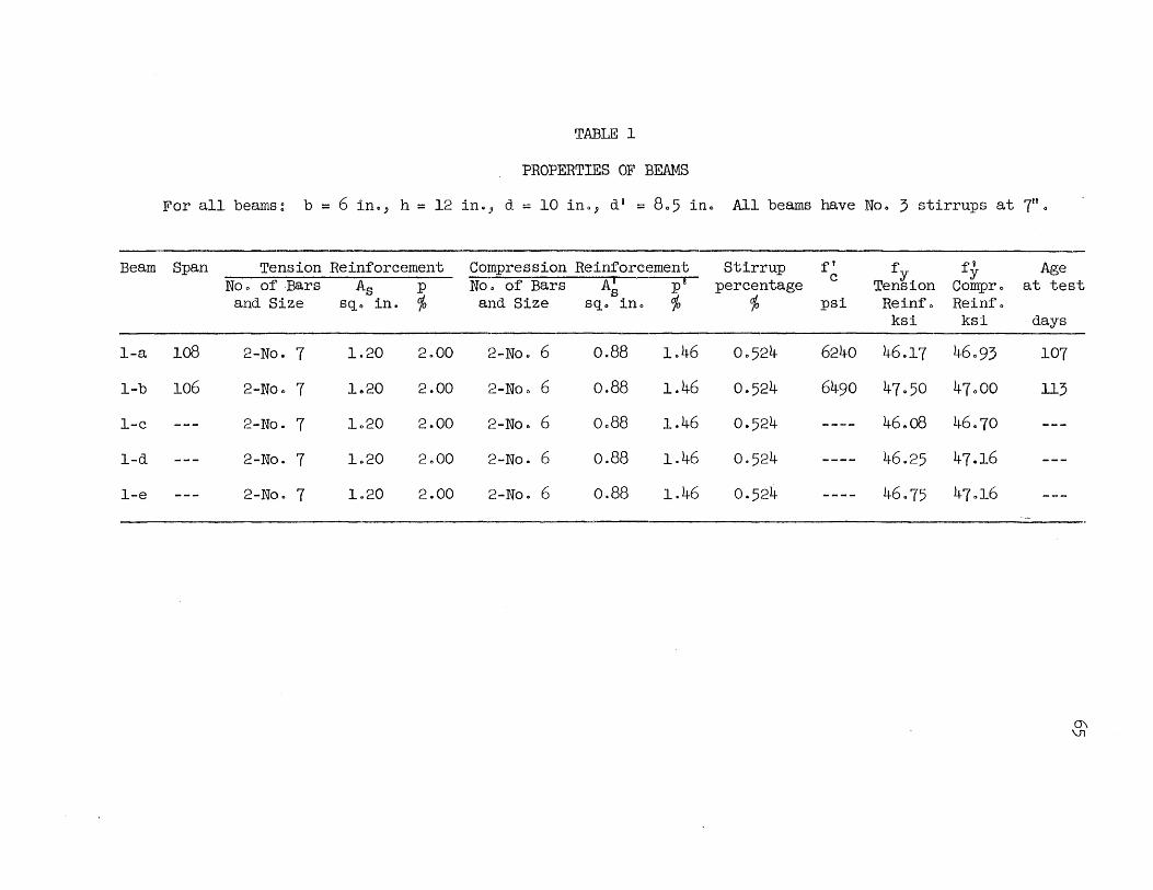
Beam
I-a
I-b
l-c
I-d
1-e
TABLE I
PROPERTIES OF BEAMS
For all beams: b = 6 inc, h = 12 ing~, d = 10 ino, d t = 805 ino All beams have No .. 3 stirrups at 7ft"
Span Tension Reinforcement Compression Reinforcement No". of Bars Ai p8 Noo of ·Bars As p s
and Size sqo in. % and Size sqo ino %
108 2-No. 7 1.20 2000 ~2-No" 6 0.88 1046
106 2-Noc 7 1.,20 2.00 :2-No 0 6 0.88 1.46
2-No. 7 1020 2 .. 00 :2-No 0 6 0088 1.46
2-No. 7 1.,20 2000 :2-No. 6 0.88 1.46
2-Noo 7 1 .. 20 2.00 :2-No. 6 0.88 1.46
Stirrup f' fy C percentage Tension
% :psi Reinfo ksi
00524 6240 46.17
0·524 6490 47g50
0·524 46 .. 08
0·524 46g25
0·524 46.75
fW Y
Compro Reinfo ksi
46093
47000
46.70
47.16
47,,16
Age at test
days
107
113
0\ \Jl
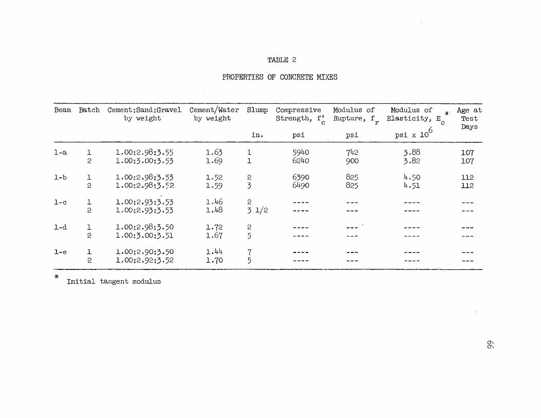
Beam Bateh Cement~Sand~Grave1
by weight
1-a 1 1.00g2098:3055 2 1.00~3000~3053
I-b 1 loOO~2098:3o53 2 1 .. 00~2098~3o52
1-c 1 1000:2 .. 93:3053 2 loOO~2·93~3·53
1-d 1 1000~2.98~3050 2 1.00~3·00:3051
l-e 1 loOO~2090:3.50
2 1.00~2092:3·52
* Initial tangent modulus
TABLE 2
PROPERTIES OF CONCRETE MIXES
Cement/Water Slump Compressive Modulus of by weight strength, rw
c Rupture, r
in. psi psi
1.63 1 5940 742 1.69 1 6240 900
1052 2 6390 825 1·59 3 6490 825
1.046 2 1.48 :3 1/2
1·72 2 1067 5
1.44 7 1070 5
Modulus of
r ElasticitYj E
psi x 106
3088 )082
4050 4051
* c
Age at Test Days
107 107
112 112
0\ 0\
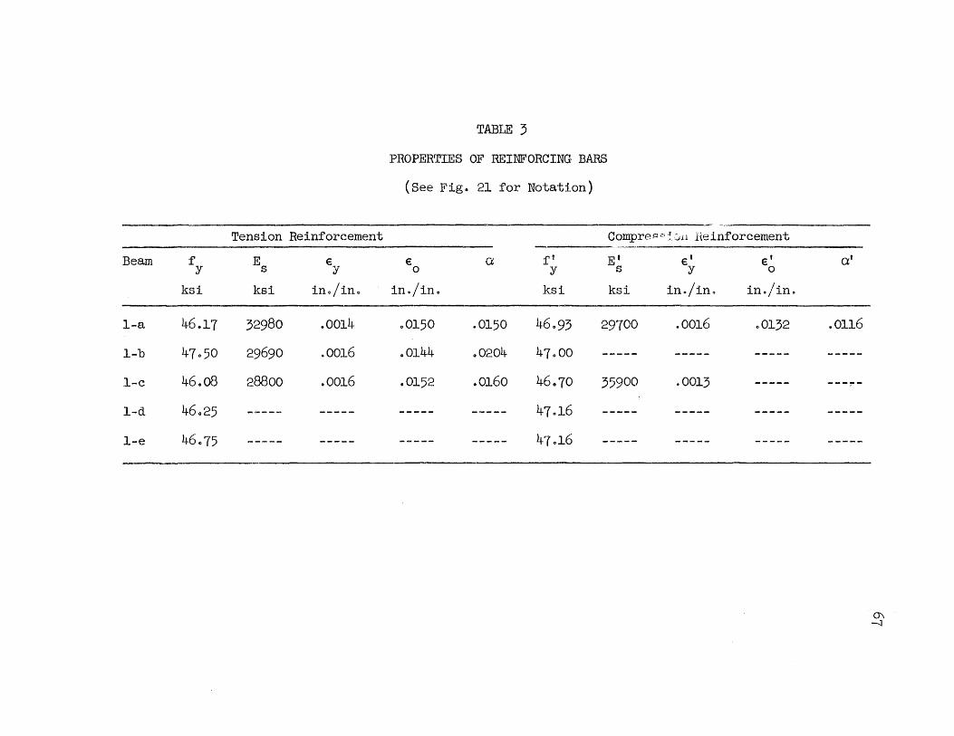
Tension Reinforcement
Beam f E e y s y
ksi ksi ino/ino
I-a 46.17 32980 .0014
I-b 47050 29690 .0016
I-c 46.08 28800 .0016
1-d 46025
l-e 46075
TABLE :5
PROPERTIES OF REINFORCING BARS
(See Fig. 21 for Notation)
Compre Fl '" ~V.ll Heinforcement
e a ft E' e' e' 0 y s y 0
in./ino ksi ksi in./in o in./ino
00150 .0150 46 .. 93 29700 .0016 00132
00144 .0204 47000
.0152 .0160 46070 35900 .0013
47016
47016
a'
.0116
0\ -:)

TABLE 4
TEST RESULTS
Beam Span Natural Loading Failure P P M M 6. 6. L Period, Rate Side y max y max y max
T North South
ina milli- kips/min 0 kips kips kips ino -kips in~-kips ino ino seconds
(1) (2) (3) (4) (5) (6) (7) (8) (9) (10)
I-a 108 18 13 N 2304 23a2 3000 559 720
1-b 106 18 15 s 2303 23.3 2904 548 691 0·35 6
8i

Beam
l-a
1-b
(1)
(2)
(3)
(4)
(5)
TABLE: 5
INTERMEDIATE qUANTITIES IN COMPtrrATION OF MOMENTS AND DEFLECTIONS
n k" k' f f' cry w L gl f c s s E d t
Eg. 2(1) (2) (3) (4) s
Ego 3 Ego 4 Ego 6 = - == -E d c psi psi per 'inG ino ino psi
----8063 0.85 0.394 3360 17960 0000231 12 loB 0.0382 67,350
6058 0.85 0·364 3980 15400 .000252 12 106 0.0407 69,160
Equation numbers refer to equations in Reference 20
Width of column stub
q' = (pf - plfl )/f' Y Y c
f = M /.J~ d t
s max s
~I = (pf - plft )/f ' s Y c
q"
(5)
0.106
0.107
0\ \0

TABLE 6
COMPUTED MOMENTS AND DEFLECTIONS
Beam M 6. M 6. M Y Y max max y
Eqo J-(1) Eqo 7 Figo 81 Figo 82, measo in-kips in. in-kips in. , .... compo
(1) (2) (3) (4) (5)
l-a 479 0.25 687 703 1017
1-b 497 0.26 705 703 1.10
(1) Equation and figure numbers refer to Reference 20
6. M y max
measo measo compo comp.
(6) (7)
1.05
1·35 0·98
6. max
measo --compo
(8)
0.82
-l o

TABLE '7
v ALVES OF RESISTANCE AND LOAD CHARACTERISTICS USED IN ANALYSIS
Resistance Chara,ctei'Ts-:fTc-s- Loa,d-Characteristics Probo ~ ~x 6. 6. T P t t td P/Q Noo y max r p y
kips kips ino inc milliseco kips mllliseco milliseco mil1iseco
1 2501 2602 0034 707 23 1902 701 702 701 0.76 2 1403 3 3507 4 3201 702 1028 h 1403 .J
6 3507
7 5103 702 2004 8 1403 9 35 .. 7
10 2406 2508 0·38 505 25 1809 703 703 7·3 0077 11 14c5 12 3603
13 3105 703 1.28 14 1405 15 3603 16 5004 703 2004 17 1405 18 3606 5804 0.40 600 20 28.2 609 609 609 0077 19 1308 20 3405 21 47·0 609 1028 22 1308 23 3405 24 7502 609 2006
25 3502 3602 0.46 306 23 26.,7 7·2 703 702 0076 26 1406 27 3603 28 4405 703 1.26 29 14.6 30 7102 703 2002 "j::l

TABLE 7 (ContVd)
Resistance Characteristics Load Characteristics Probo Qy ~ax 6 6 T P t t td p/Q
Noo y max r p y
kips kips ino ino milliseco kips mil1ilsec D milliseco millisec.
31 2501 26.2 0034 707 23 1902 10 10 10 0·76 32 20 33 50
34 32,,1 10 1028 35 20 36 50
37 51.,3 10 2.04 38 20 39 50
40 24.6 25 .. 8 0.38 5,,5 25 18·9 10 10 10 0 .. 77 41 20 42 50
43 31·5 10 1.28 44 20 45 50
46 50.4 10 2.04 47 20
48 19·3 20.3 0.21 7·8 23 3104 10 10 10 1.63 49 20 50 50
51 2102 2202 0 .. 29 7·7 10 1.48 52 20 53 50
54 2301 24 .. 1 0.,32 106 10 1.36 55 20 56 50
57 25,,0 26.1 0.35 705 10 1.26 58 20 59 50
60 19·3 2004 0026 109 lO 1.63 61 20 -..:]
62 50 (\)

TABLE 7 (Contid)
Resistance Characteristics Load Characteristics Probo Qy ~x 6- 6- T P t t td pl~
Noo y max r p
kips kips ino inc mi11iseco kips milliseco milliseco milliseco
63 2103 2203 0.29 7.8 23 3104 10 10 10 1048 64 20 65 50
66 2301 2402 0032 707 10 1.36 67 20 68 50
69 2500 2601 0.35 706 10 1.26 70 20 71 50
72 19.4 20.4 0.26 8.0 10 1062 73 20 74 50
75 2103 2204 0029 709 10 1.47 76 20 77 50
78 2302 2403 0.32 708 10 1.35 79 20 80 50
81 2501 26.2 0034 707 10 1.25 82 20 83 50
84 1904 2006 0026 802 10 1.62 85 20 86 50
87 2104 2205 0028 801 10 1.47 88 20 89 50
90 2303 240·4- 0031 8.0 10 1.35 91 20 92 50 ~

Probo Noo
93 94 95
501 502 503
504 505 506
507 508 509
Qy k:lps
2:) 03
2501
TABLE 7 (Concluded)
Resistance CharacterIstics Load Characteristics
~x £::., £::., T P t t td y max r p
kips ino ino milliseco kips mil1iseco mi11iseco mi11iseco
2603 0034. 709 23 3104 10 10 10 20 50
2602 ~085 707 11 3104 10 10 10 20 50
0170 16 10 20 50
0255 20 10 20 50
P1Q y
1024
1025
--:J +-

75
TABLE 8
KEY TO COMPARISONS OF ILLIAC RESULTS
Fig. No. Variable Remarks Constant
39 Qy' effect of steel t = lO milliseconds P p
yield point
40 t1 t 20 n P = P
4l n t = 50 n p p
42 ~, effect of concrete t = lO It P P
strength
43 fI t 20 " P = p
44 It t 50 tI P = p
45 6. , change in initial t = lO It P y P slope of resistance diagram
46 11 t 20 f! P = p
47 If t = 50 n p p
48 t , load duration P = 1902 kips Resistance p function
49 n p = 3l.4 kips "
50 ft P = 5l.3 kips 11
5l P, load magnitude t = lO milliseconds II
p
52 " t 20 ft If = P
53 u t 50 n tI = P

,,=+r-~~T-t-~~Lj!=r=!r:r--- CrnNECTING BAR
'-++~.---- TRIGGER SUPPORT
,L_il====::::iL~J::=====ill_~---AUXILIARY CYLINDER
--PRESSURE HEAD
-----t+~-+---"-- - - SLa: vAL. VE CYLINDER ORIFICE
--SLDE VALVE CYLIt«R
--STORAGE CYLINDER
INSERTED HERE
~~~g=====~~~~r--- -STOP PLATE
-MAIN CYLINDER
MAIN PtST~
AUNEMENT PLATE
SLDE VALVE 1"'"""W.,.,.......:-4L-I~._/ CYLINDER ORIFICE
/SLDE VALVE CYLINDER
~~-+----- ·--SLIDE VALVE
'-SLIDE VALVE ROO
-----PRESSURE HEAD
~~t::1t-f,fFT-·-AUXILIARY CYLINDER
~'-.I==-----AUXILIARY PISTON ~"""oo-:!iII
RESET
A
rCTIJ"qm-- ---AUXllIARY CYLINDER ORIFICE
rJ----+-4'+---f?F-----SLIDE VALVE RESTRAINING LINK ASSEMBLY
---TRIGGER FRAME
\ TRIGGER IMPACT ADJUSTMENT
SEAR \ TRIGGER PISTON ASSEMBLY
-TRIGGER ADJUSTMENT ARM
SIDE VIEW OF TRIGGER MECHANISM
SECTION THROUGH MAIN CYLINDER
o 2 4 6 i2 L___ I
A
-----MAIN SHAFT SCALE IN INCHES
SECTION A-A

FIG. 2. TWO VIEWS OF TRIGGER AND AUXILIARY PrsrON ASSEMBLY

FIG. 3. VIEW OF CONTROL PANEL OF THE PRESSURIZING SYSTEM

f'--~-------
9J "'--- -
~I ~-~ _____ -
I I I I ----
'I I I
I I I
PI
I I I I I I I I I I I I I I
I; , I I I _____ 1
3 I I I I I I I I I I
2 I I I -------' I
I I I I 1
I r-- ---- --I
1
ror no load P2 ~ 1.11
However, the face of gage No. 3 has been redrawn to indicate pressure 0.894 times the aotual pressure. Therefore if the readings on 2 and 3 are the same, there 1s no load on the piston.
I
-----1 I I roo in
:0 I I
-----1
08UX
II
I I I main
i0 I I
IQ--.Jr~ LJ 3 '<-'
~ 1
I I r-Lf; ~ cD : 9-:~ f0, L_ 1 I
<f !
I ,
I
~ • 0~------~ ~ ~ ~ ~ ~
1-2 L_2-3
I I
I I I aux
:0 PRESSURE
GAUGE
I : ~ I r4 I Gb LINE VALVES
L ¢ ~ I BLEEDER VALVES
I r------0-o ~ o LL
~ C i I I I I 2
~II~ Z <X: ~
1-3
1 1-4
I I I 3
I 111---0--
t- 4
i III 4 rz>-
:"1110 1: 1 I
~~ -~ I II
SUPPLY VALVES
LINE INTERLOCK VALVES
FIG. 4 SCHEUATIC DIAGRAM OF CONTROL PANEL
PANEL INTERLOCK VALVES

Q)
> .r-! til til Q)
H
~ o o
p
Time (0.002 seconds per cycle)
FIG. 5. OSC lLLOORAM OF LOADrnG pITr ·SE PRODUCED USING lrrTROOEN
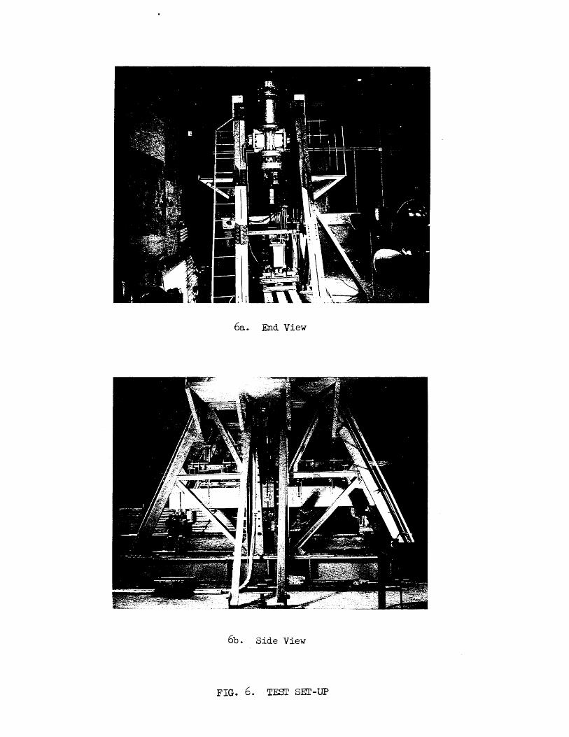
6a. End View
6b. Side View
FIG. 6. TEST SEr-UP

\ T~
LI C - Vert. Gage
o[Jo -T - Hor1z. Gage
DYDalDOmet er No. 1
o DynaIOOmeter Ho. 2
FIG. 7. CROSS-SBCTIOH, GAGB ARRAlIlDIB:MT, AJI)
CIRCUITS FOR DYHA)I)UXTERS 1«). 1 AIID 2

FIG. 8. VIEW OF REACTION-MFASURING SUPPORr
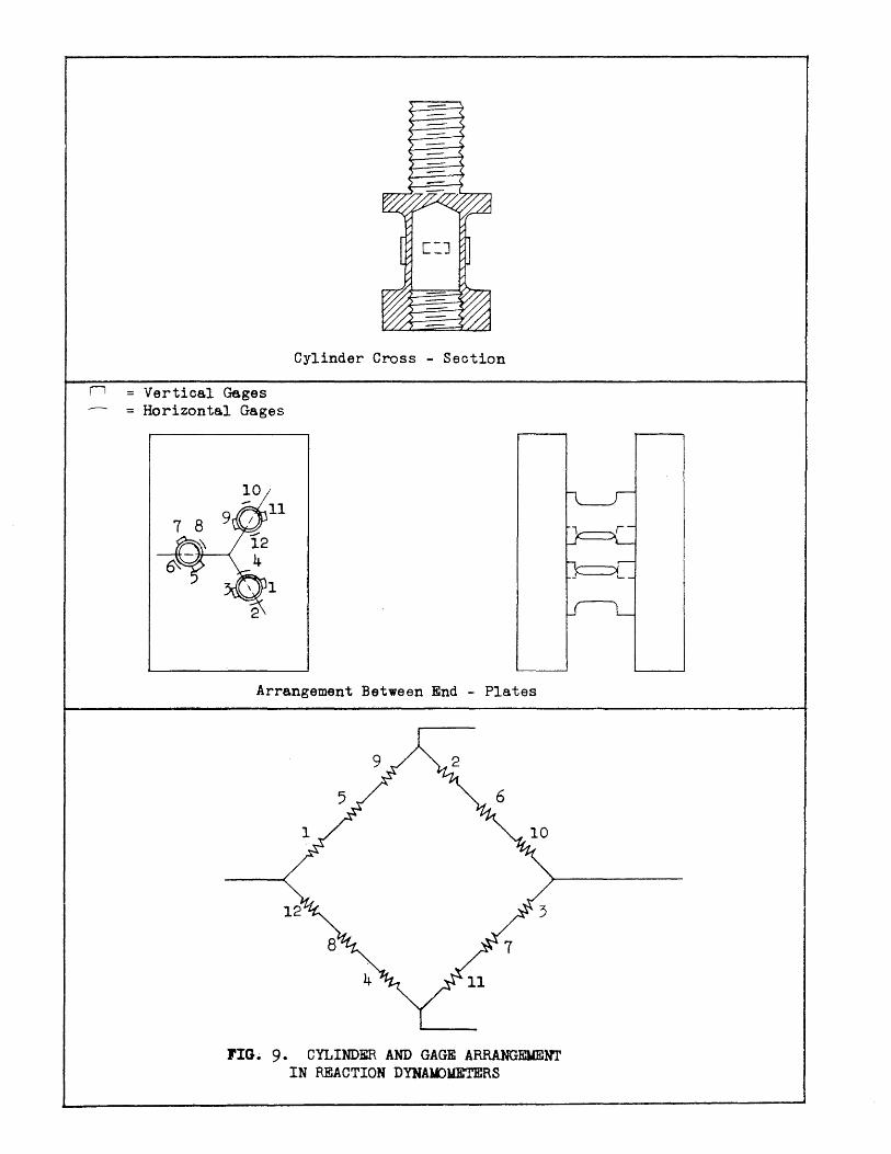
11 Vertical Gages Horizontal Gages
Cylinder Cross - Section
Arrangement Between End - Plates
rIG.; 9. CYLINDlm AND GAGE ARRANGEUENT IN REACTION DYNAUOUETERS

""'&' ~~, t~ ,'try \, " : ~~, t t , ~.
... .. ~ l:.
I
FIG. 10. TWO VIEWS OF REACTION lJYNA1.I)METER BLOCK m GRIPS FOR APPLYING TENSION AND SHEAR

oscg
-=-
-0 ~
t--.... - to
Reaction B
25 Standard Resistances
oscg
Dynamometer No. 1
v - Vert. Gages H - Horiz. " oscg - oscillograph
to oscg
Switch ----~ Variable
Capaci tances
FIG. 11. CIRCUIT DIAGRAM FOR LOAD AND REACTION DYNAMOMETERS

~unting bracket
~" ", <,,"+ 0( .
t Q •
o
• 0
slide wire
fiber block
slide wire
to recording devioes
slide rod
FIG. 12. DEFLECTION GAG!:
ball and sooket Joint
defleotion braoket
to recording devices

1
v
h ~~ lL. '
Def1eotion Gages
2
Denscltion Calibration Boards
(a) SohEnnatio Diagram of Ciroui t
~ 1& 4vJ 2 ~---r--.....J 3 L-' --r----' 41-.' --r--~
(b) Idealizeld Sohematic Diagram of Ciroul t
FIG. 1;. DElli'LECTION GAGE C:IRCUIT DIAGRAM
51-.' -~---'
v
~ V
• V
V :II power Inpu t G = signal output
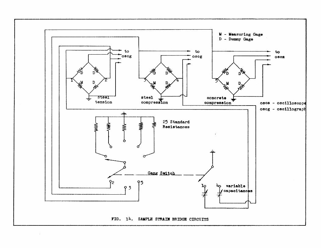
e tension
."0 a"
25 Standard Resistanoes
to 0I80g
--; ,L-~- -.-~~~-
1--__ ._~_2 _J' r
U - Measuring Gage o - Dummy Gage
r---------------~
. ..,
ooncrete
to 080 •
oompression -,r
0808 - oBol110scop 080g - osolllograp
variable capaoitano.s
FIG. 14. SAIIPLIC STRADf BRIDGE CIRCUITS

I I I I
Acceler V.l.U'.o V'-.L
1------- _______ J phase shifter 1--'
L...--__ --.-;.._, --II I
I I I I I I L __ .J
FIG. 15. ACCELEROMETER CIRCUIT
Calibrating Resistances
,carrier to amplifier and then galvanometer

FIG. 16. VIEW OF OSCn.LOORAPHS AND TIMING DEVICE
FIG. 17. VIEW OF OSCILLOSCOPES AND CAMERA

FIG. 18. VIEW OF MAIN SHAFT TIP AND BEAM CAP
FIG. 19. VIEW OF MISCELLANIDUS EQUIPMENr

54
52-1/2
16-No. 3 stirrups at 7 starting 3-1/2 in. each side of centerline
3 1/4 -
1-1 /2 b...--4 11 11
8-1 /2
4 6
52-1/2
2-No. 7
L
2-No.6
;( I rl-1/8
I
I
19-5/16
? stirrup - No. 3
c ~-9/16 \ 2
3-1/8 \2-4 . No 7
Section A-A
FIG. 20. STEEL REINFORCEMENT DETAIL
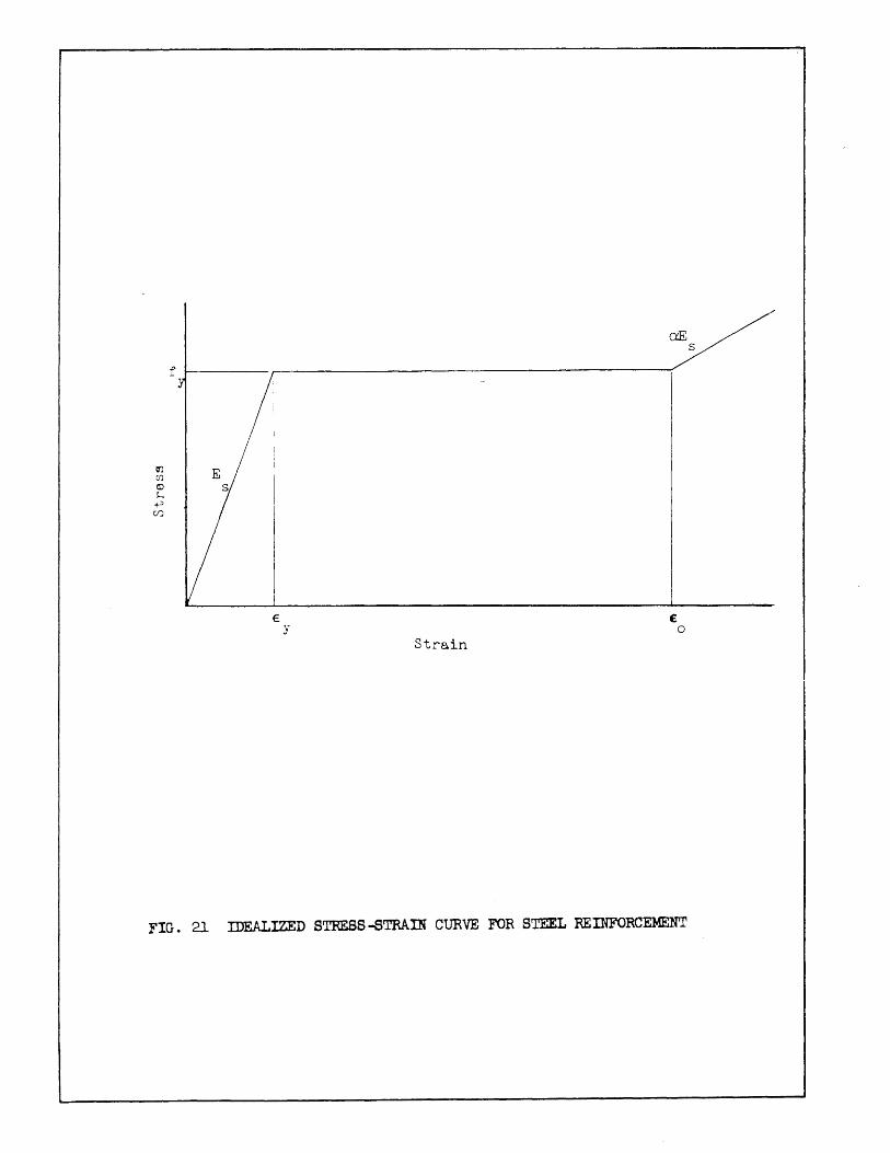
aE s
+' ':'y
0') E [f)
CD S h ~ (/)
€ £ Y 0
Strain
FIG. 2l IDEALIZED STRE8S-8TRAIN CURVE FOR STEEL REINFORCEMENT

Bar Ground Gage M;:>unted
Leads Soldered Gage Waterproofed
." ~ • ~ • .., ....... '" "..-41" •• I' "' __ !!.
:. # .., ~ :' :'" tI.. ' ........ .
Waterproof Test
Assembled Reinforcing Cage
FIG. 22. srEPS IN FABRICATION OF REJNFOR!lN} CAGE
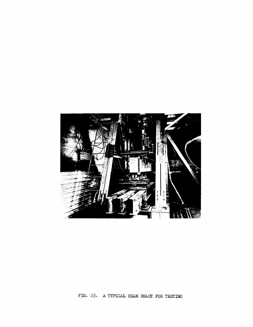
FIG. 23. A TYPICAL BFAM RFADY FOR TESTING
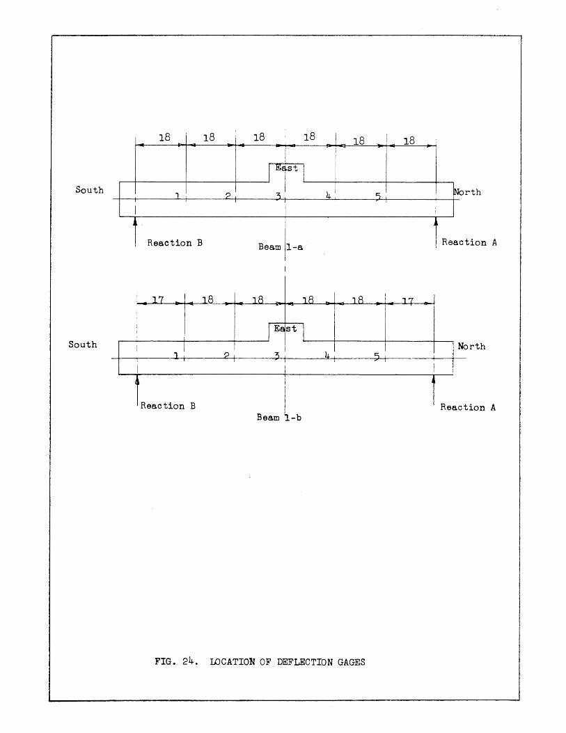
18 18 18 18 J ]8 I 18 I
I I I
i I I
I bj~ st 1 South , , ? -;z; k ~ No rth
I
I i j t
Reaction B Beam I-a 1 Reac tion A
South I North
Reaction B Reaction A Beam -b
FIG. 24. lDCATION OF DEFLECTION GAGES

17 I 7
Compression Steel I I
., ... SO I - SQ I
..c: SP_ _ SR ..c: ~ -s... ~
~ ::l 0
U)
7 7
Tension Steel
SA- -~ SC I
I SD SB R .... I
I
Beam I-a.
Concrete I-- .- - - - - - - - - -00 - - - - - - -=-+ - - - - - --
CA."... + £,C Irl",CD t 3
~---------- '- -- r-- - ---------2 7 7 7
7 7 7 7
Compression Steel
scr"" S'P I SQ SR
..c: - II ..c: ~ ~ r... ::l
~ 0 tI.l
7 7 7 I I I
Tension Steel
Sv SD ~B I
-
Beam I-b
FIG. 25. STRAIN GAGE LDCATION

West Side
East Side
FIG. 26. BEAM l-a AFl'ER FAILURE

West Side
East Side
FIG. 27. BEAM l-b AFrER FAILURE

301 /~
25/ 7V' ---j
2°1 / 1 ~
\ ill Y Y Pl ;1 15
.... rd
S IRa+I\~/ ~~ Ra
10
5 I ~L I 7( :701/ ----1
o~ o ~ 2u 40 60 120 140 80 100 160 Time, seconds
FIG. 28. LOAD AND REACTIONS VS. TIME, BEAM l-a

ill PI
"r! ~
25
20
15
cd .... 10 cO o H
5
o
~ 'I
~ ~
o
i...---""
II se
11 ____ SA
l--------l----SB, SD
E Y I
.002
~ ~ SD"
,
-.006 .004 .008 .014 .016 .010 .012
Strain, inches per inch
FIG. 29. LOAD VS. TENSILE STEEL STRAIN, BEAM I-a

ill P-! ·rl M
rd" cd 0 H
30 ===il
~ ~~ 251 ~~- \So
I I I I
---- SP
20 I ~ II ----t
15
I
10 m ~ --
, ~
I
VI , E
Y
+ 0 .002 .004 .006 .008 .012 .014 .010 strain, inches per inch
FIG. 30. LOAD VS. COMPRESSIVE STEEL STRAIN, BEAM I-a

2CJr------
20
I CC
I !7ILlCB 15
rJ]
Pi .r! ~
cd"' cO 0 10 H
)~I~<_------+------------r----------~------------~----------~-----------+----------~--------__ ~
.0005 .0010 .0015 O~. ____ ~~~ ________ L-________ L-_ o .Ou20 .0025 .0030 .0035 .0040
Strain, inches per inch
FIG. 31. LOAD VS. CONCRETE STRAIN, BEAM l-a

en 0.
orl ,!.4
...
30
I I 1 I I I Ra. + Rb
I
I I I I I I / 25 .
I I I
201
R 151 7/7/ d.~
R, B.
] lOL I --~ dj~~_- . I ~---~-
51 + I +----i I
O!~ I I .l ~ o 20 40 60 80 100 120 140 160
Time, seconds
__ . .-!IG~l?~~ A ~~~~. __ ~~~~_~~~~~ . __ ~~ .... ~~~_'-_~~~~ __ }-_=-~ _____________ ._~ ___ ,_. ___ . __ .

30
25
20
to
~ ;r4 15 rd~
cd o H
10
5
o .002 .004 .006 .008 ,,012 .011+ .016 .018
Stra.in, inche s :per inch
FIG. 33. LOAD VS. TENS ILE :STEEL STRAIN, BEAM 1-b

30
25
20
(})
Pi 15 'n ~
"' ~ o H
lO
5
o
'- so , 1
..
E Y I
o I
I
~SR I
I
E 0
I .002 • OOL~ .006 .008 .010 .012 .01)+ .016
Strain, inches per inch
FIG. 34. LOAD VS. COMPRESSIVE STEEL STRAIN, BEAM l-b

3()~----------~----------~--------~-----------'----------'-----------'----------'-----------'
2 1-1 ) J
201 11 / 1//
(J)
~ ·rl ~
rd"' 115 tU o H
101 / / If
151 I h'
.0005 .0010
17 I:::::;;»="
.0015 .0020 .0025 .0030 .0035 • OOL~O
strain, inches per inch
FIG. 35. LOAD VS. CONCRETE STRAIN, BEAM l~b
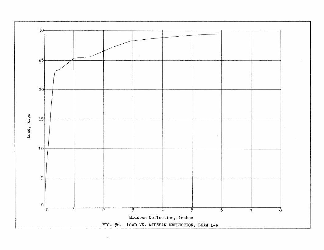
30
25
20 I
til P. ~ 15
'"' rc1 cO .s
10
5
o
I I I I
I
~ ~
/
I I I
- -4 -3 5 7
Midspa.n Deflection, inches
FIG. 36. LOAD VS. MIDSPAN DEFLECTION, BEAU I-b

m ~ ~ u Q H
2 0 ~ ~ u ~ rl ~ ~ ~
1 2 3 4 5 South + + ~ + + North
~ 8'-10 r 0
2
3
4~------~----~~--------+-------~~~--~------~
5 ~------~--------~--~~~~---7~--------~-------
6 L--------L------~--~~~~~----~------~------~ Midspan
FIG. 37. DEFLECTION SHAPE AT VARIOUS PERCENTAGES OF MAXIMUM LOAD, BEAM I-b

OL-______ -L ____________________________________________ ~~ __ __
Deflection, inches
Resistance Function
P~------r__----------------_.
t r
t :p
Time, milliseconds
Load Pulse
FIG. 38. NATURE OF RESISTANCE FUNCTION AND LOAD PULSE ASSUMED IN SINGLE-DEGREE-OF-FREEDOM ANALYSIS

Q) 0. ..... ~
... a
... to 0 s:: ~ to
..-4 rt) (0
a:=
rt)
0. ..-4 ~
... 0...
"' ~ ~
S
CD CD .c 0 c
..-4
<J ...
s:: 0 .~
~ 0 CD
C CD
0
50
40
30
20
10
o 0
50
40
I I
81 I i
I I i I I
I
r 78 I I I
I [ ! I ---;---
T I I ! I
75 I I ; i I I I
72 I I I
I i I i I 1
I I I . -f--J- ----r--~- -~ I I I I
I ' I
I i
I I 1
I i 1 I
, I I 1 i I
1 2 ·3 4 5 Deflection,~ , inches
1- -.---r----, --,------·1--1
I i I I i +------+--+---r----f--~--+_~~_+_-~-t--- L - ~ J
30
I 1 I: I I
t------:-.:::--=--=-~I--+__- -----+----L~-~--L_1~ ~~b~tS. I : II I 78, 81
20
10
i I I ' I . I I
I -+- I
+-+--+----+----+----4-----+1--- . --1 I I ! i
-+---\--+---~--~--+---Lt ----+-----.--... ----------, ,
I I I I I
I I
10 20 30 40 50 60 70 80 90 Time, t, milliseconds
10 -'---I'-~!
8 ~--1~--j I I
I I
6 I I I I
--+--"1 I '
4
2
o 0 10 20 30 40 ~ 60 70 80 90 100 Time, t, milliseconds
FIG. 39. EFFECT or STBL Ym..D PODT 01 RESPOJ(SE: tp. 10 MILLISECOlmS
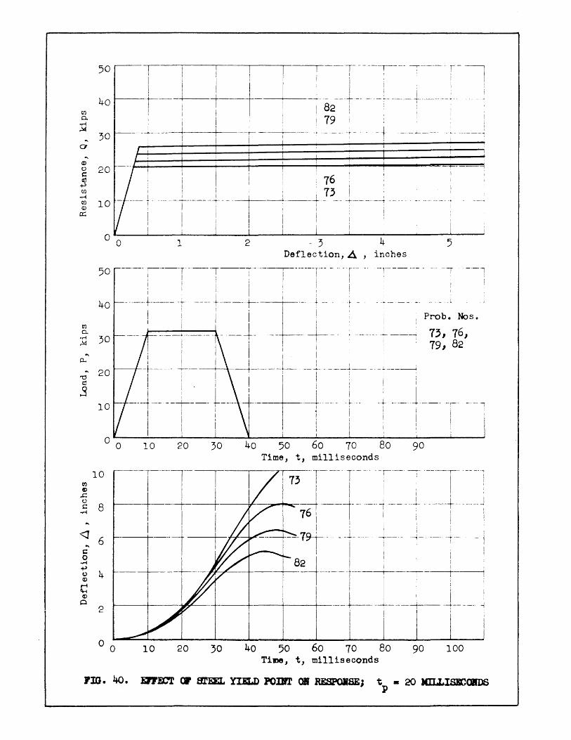
50 r---i I I I 11---------:---- i-------- r-i I iii Ii:: i I !
40 _',I -+-, i,--t-+-~,'--82---t, -- ----~,-------+-------.--- ~ til ! I I I I I I i
0. I i, I I ! 19 i ' : ' ~ I I", :
~~ 30 iii ~------t---- --+---+------i----~ a l I I I I
~ I~Cj ====1~--~---41----4----+----~---t_1--~_===!:===: I- I i ~ 20~--1~+===~,----~!---~I---r--~---------+T----~~~rTI-~~
~ i I I I I 16 I I
~ 1 I : I '13 i ; i
~ lo-r----r-Ti--r- r-- l ------o 0
50
40
Ct)
0. oM 30 ~
.... 0..
"' 20 "0 ~
1 2 3 4 Deflection,~ , inches
----- r- ---r----i--1- ---T------ r -- - - -r--- -- --1 -- --- ---r
I I I I I
I I I I I I'
i I I
---r------ i --r--t ------+------- - - --1- ----+---
: I
~ - -I
I
-------!
I i ! I Ii' :
-t--------t-- --T-- ----t--- -- -t---i t---~--+----- -- -- --,------i
i . I I I
I
5
_I
Prob. Nos 0
13, 16, 19, 82
I I
---1------- - I ---J----S
10 I
t---I-----.-+ ---- ----+--- ---I i I
I !
o 0 10 20 30
10 ----·T-·---l--j en
---t--~--+ CD .c 0 s:: 8 ~
I I I <1
I I
6 1-1 I ....
c 0 ~ -+---+----~ Q 4 CD
C CD
Q 2
I J/I a 0 10 20 ;0
40
40
50
I • I
i I I
60 70 Time, t, milliseconds
50 60 70 Time, t, milliseconds
80 90
80 90 100

CIl a. ~
~
... a
... ;)
0 s:: ~ ~
CIl ~
C1.l m
a::;
CIl a.
...... ~
.... 0...
"' "0 ~
.s
O'l ~
..c: 0 t:: ~
<J ...
t:: 0 ...... ~ 0 ~
C ~
0
50
40
30
20
10
0
50
40
30
20
10
0
10
8
6
4
2
.------r- 1 t--r ----~---I i I I
Iii I
~-+- ! ! i I i -8-3--+----1 -- --- i ---1---- -------1
! I I , I I 80 Iii · i I
~---+-----+------~>---__+____---_4-----t-----t--- -+--- --l~ !
f I ; I I 1
, --F=~
! i I I
I ill
1 T ~ : -i -- - :
:
I ---+--- --I I
I
I iI : I ; I : --l--lIj
i ---r--11i --or - ;-- -; I i I I
0 1 2 -- 3 4 5 Deflection,~ , inches
-T---r----r--r --:-- r -or ' -- ----+---- -+-- ---- r ------l----t--- ~ - ---~- -- - ~- -- --- -~ -- _1. ._-- __ .1
I I I I I )
Iii i i Pro b. No s •
I I I ------'. ----i--------:- -L ----~.-- - 74, 77,
I----I----+_ c---~-J--1-- I ! __ ~ 80, 83
! I I I -------~ ---~--+--l-I I I I I I I I
0 10 20 30 40 50 60 70 Time, t, milliseconds
80
I
+--
90
-i-~-~j=r---1-----
o 0 10 20 ~o 40 50 60 70 80 Time, t, milliseoonds
90 100
FIG. 41. EFFECT OF BTDL YIELD POIBT ON RESPOHSE: t - 50 MIIJ,I8ECOBDS P

50IT III " -r-T-T---n 40 .----r--+-i --+----+-1/--+---90-+1----+---+- r---t---i
~ I" 78 ,: I ! ! " I -r1 I iii ~... 30 "------+---+-----+----+-----+---_11--- ---t---- i -+---+---~ a i [I i ! J
... I' I I I ! i I
~ 20 ' ---t------f,---ir--66!- --;--1---+--- i i
~ 10t----;I--------1'--T,11 - I J~J---l---1-----j--------J-----~ 0:: : I' Ii [I i ~ i : :
i li i ! o 0
Cfj
0. • .-1 ~
... 0....
... -0 cO Q .....
0') QJ
.c 0 ~
-r1
<J ... ~ 0
• .-1 ~ ()
<D
C <D
0
1 2 3 4 5 Deflection,~ , inches
50 -r---T----r-r-~i----T -r--! --r
I , i I I ! :
-------~-------:------+- ------t---j ---+ -----~---- ---4 -- -- - +
i I I ! I I I I
40 - - -j
30
20
10
o 0
10
8
6
4
2
o 0
-- ---11
-- --T-r---i-- --. -- ~ -- -I I ! ! : I --4----~. - I-t -- ----1 ____ --1 ___ ----J I I I I I
Probe Nos.
54, 66, 78, 90
I Ii'
-r---+ -t----l---r--i- ... I I !
--+ - - --- - 4--- - ------, i
10 20 30 40 50 60 70 80 90 Time, t, milliseconds
10 20 30 40 50 60 70 80 90 100 Time, t, milliseoonds
FIG. 42. EFFECT OF CONCRETE BTREBGTH ON RESPOBSE: t - 10 MILLISECONDS p
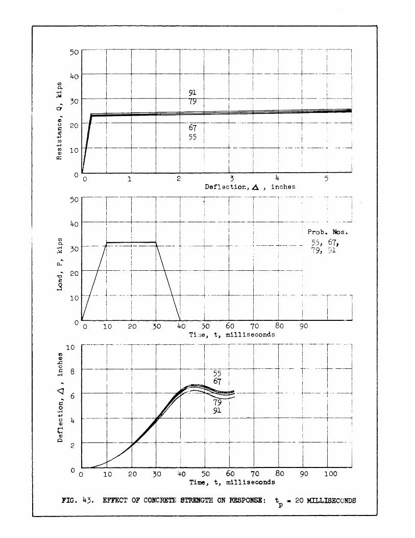
CI)
0-..-l ~
.... a
.... G:) 0 t: ~ ~ CIJ
..-l OJ CD
0:;
OJ 0-...... ~
.... 0...
... -0 ~
S
~ G:)
.c 0 t:
..-l
.-"I
""" .. t: 0 ...... ~ 0 CD
C CD
Q
50
40
j I 91 -J-(';j 30 i I I I
-T--II I I I I I --+----+----+-, -i---t----r-- ---I
I I : ' ! I r ! ! I i I
"?Trr-+----t--~---+--t - --f----l I I I, !
I
(-_ I 20 ~I 67
~---t-----T~-55
10
I I , I
I _+_ ' i ! --+------+---+-----+--------+-. --. -+--- ._---+_._- --~-- --~
! I I t i ; I II i I
I I : ,
, i I : , : ~ __ I I ---~ __ u,_~ l 1 ;: J
o 0 1 2 3 4 5
50
40
30
20
10
0
10
8
6
4
2
Deflection,~ , inches
--r--T--l---r--T-~r-T---[---:- .-[ ------1---+----+----t-.-+- --- ;---+-.--+---- -; .. ... .-l ii' i I! i Pro b • No s • -----"--- ---1. --L---+--- -.---- 55, 67,
I 'i I 79, 91 ! I I ' I I I I I '
-.... ----+---\----i---.- ---.~---+ -+----i-- - --~
i----l---+----\--1-1
__ l __ 1-_i ----ti
-- J-- r---- , I I I i I
: i . I ! I i J o 10 20 _30 40 50 60 70 80 90
Ti2e, t, milliseconds -- -r----·-i~
--r- ---l
I !
----t- --l ~--L-t--
.-- --
! I
I i
----+---+----t-55+~ -t---t-·
~-1-·----
10 20 30
I I I I , I +--- .. ~ ... --__ J i t I
67 I ~~~ I I
~~~~ ------1--.-... -+- - . I I
79 i I I !
___ 1_9_l
+1--~-+~-I-r--:
--- ----t---l-- .~ I
40 50 60 70 80 Time, t, milliseconds
90
I
100
FIG. 43. EFFECT OF CONCRETE STRENGTH ON RESPONSE: t =- 20 MILLISECONDS p

I I I I I I
40~--~----~--~----~--~----r----~---~----+11---:-----
;l II I
~ I I I
~... 30 I 80 --+ I I
a ~1~~~~~~+-1--t-1--r-, ... ". 68 I I i g 20 I 56 ----~----+--t-I I, i r!1 ' I I
~ 'I I I I ~- I 'I i I I
~ 10 l~ ---;i----I !, ---+----4----+------+--- --+-----t--t--i-------l
~ I ' I I I I j I ! I
50
I
o 0 4 5 1 2 3 Deflection,~ , inches
50
40
0)
0.. -H 30 ..'l4
T---r -- I -r-i---r - --j __ u ~---i--u·1
---L---J---J---+I -~----t- --+-- --.1------~ _____ L -,-----j I I I I I '
I I I : i: i Prob. Nos.
I ' --------L----- __ ~ ~;~, I ...
0..
... 20 '0 ~
oS 10
, ii, ---r I i j--J-+-[ _~I-----+----4 ----~---t---+--+--- -. t -----.-
i I I I I , I I
o 0 10 20 30 40 50 60 70 80 90 Time, t, milliseconds
10 --T Cf.l I ~ I ..c
I 0 ~ 8 --t----
-rl
! I
<1 I
.... 6 s: 0
-H +' 0 4 ~
C CD
0 2
o 0 10 20 30 40 50 60 70 80 90 100 Time, t, milliseconds
FIG. 44. EFFECT OF CONCRETE STREI«lTH ON REBPOISE: tp. 50 MILLISECONDS

::~--~--~ __ ~~--~--~I--~_-~--~---t I I I I
_ 30: ;gt I ! I ! : ~ : flit ! 507L __ +-~+-- -ri --~J i 2
100 IU_t
l __ -+--__ --+-_--+-_
8
_
1
_+_ : I ! : i
~ I/- i i iTl---T-r--:
tf)
0. oM ~
"" 0...
'"' "0 ~
.s
0')
co .c 0 c
oM
<1 "" c
0 oM
+> 0 co r-i '+-I co
Q
o 0 1 2 -. ; 4 5 Deflection,~ , inches
50
40
30
20
10
---I-l--~lr1-l----r- :---r 1 I ! I t---t----t----i--- ----~ --.. -.J
i I Iii i Prob. Nos.
--+, -~~---t'_--L_- +. '---1. 501, 504, I I Ii: 507, 81 I! i! I
I I • I i
+--+--r---------t-: --+-\ - , ----t-----.:-~ I I I I ! ;
-+---~---+ I --L---L-... t----j------~-----I I ! I ' Ii' I i
I
0 0 10 20 30 40 50 60 70 80 90 Time, t, milliseconds
10 ----1-I I
--L--8
6
Ii I, I" r---r---r-- -1--:--- 1
--+--1 -+----b--
I
-I~I- -l-- t -+~--~ I
' i I I I : I --+--_----11---_-+----- --+---- -t------ -t- ------1
Ii I ' I
----1-4
2
1 I I -~ I Iii i
+-- -+---t--j~-- ~ o 0 10 20 ;0 40 50 60 70 80 90 100
Time, t, milliseconds
FIG. 45. EFFECT OF CHANGE IN INITIAL SLOPE: t • 10 MIIJ.IBECONDS p
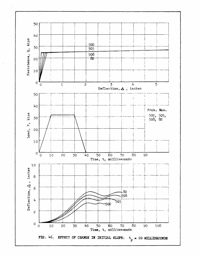
en 0. ~
~
... a
'" CD 0 s:: ~ tf.l ~ 0') (D
a::
tr.l 0. ~
~
'"' 0...
... '0 ~
S
~ ~
..c 0 ~ ~
<J '"' ~
0 ~
~ 0 ~
C ~
0
50
40
30
i I I I ~~~~~~,-1-~j-~~i-
f I i I ! i l ~--+i---t---+---+-~£....:::·~~=-5--+---+'----t-j --t-i: --+1 I
I I
20
10
Tfl ! 5~ 1: ___ ... i __
W--ifl-l-l-/_+-! --+-l--+I--+---oz~~-t--Ii ---~---r--T I j
~--:~-~n-----4-'---+----T-----+-i --T---T, -T~~\I : I I \ I!: I :
o 0 1 2 -- 3 4 5 Deflection,~ , inches
50
40
- -~- --: II I --T --T -- ----- f -- T-l -+---i---+--r -t-- ----+- --- __ + ______ L _______ J
30
20
10
Iii i i 'I Prob. Nos.
_, _ l.-_-_-_~I-----.j ____ + __ ~_-+ ___ -l __ _ -~ -~ 502, 505, I I: I' i 508, 82
I I I I I! I : I I '
1---1--+-- - -r----+.--\----------i-I---t- I I -~---~
-1--~- t++---~--+---l- T---l I I I J : : 1 ! I
10 20 30 40 50 60 70 80 90 Time, t, milliseconds
10 --- ·-··r----
8
I
6 --1-I
I I
i--r--l--r ---: I I --+---1---t--r- --r---I
--4----+- --t----:- I ----{- -- I -----~ -- ---: 82 i I I! :
08 It:
-1---4 I
2
i I
--+---+-1 - ~ i '
o 0 10 20 30 40 50 60 70 80 Time, t, milliseconds
90 100
FIG. 46. EFFECT OF CHANGE III INITIAL SLOPE: tp. 20 MILLISECONOO
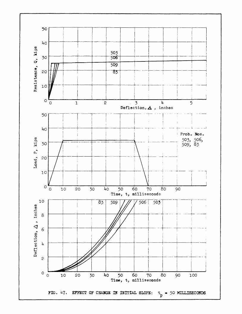
50
I Ii I"l 1 I J
~ 40~--~'----+I---+---+---+---4i----4II_--~!--~i----r--l 0. I' I ,
:Q 503 : I Ii: : ... ;0 t----+--~---+--~5~OO-+------i,·-----t I , -T-·-I
o I I I I
«>... r III I 509 I i I: i 20 -+-- ---t------+-----t----t-~ g r I (j3 I ~ I i r I
~ /I II' /' I:;! ". I I !: I
] 10 ~ ---I-----+i---+----+!---+I---+I-! r _n-r---:-i o 0
OJ 0.
OJ ~ .c 0 t: ~
<1 ...
s:: 0 ~
~ 0 <I> r-i ~
<I> 0
10
o 0
10
8
6
4
10
1 2
20 30 40
4 5 Deflect1on,~ , inches
50 60
- __ -i-- .. - _. ___ L _______ J
I Probe Nos.
503, 506, ... - --_.-+- - . ----:
509, 83
: .
---L- --+ ------.; I : I I I I '
I I I I ---r---.--.- --~
I :
--+--
70 80 90 Time, t, milliseconds
,- 83 506T---503T----l------r---·----:
+---------f-----+---+H ---+--+-1 ---t-l--~....--L---~ iii I ! --+ iii I ! i
--f ----+---,'-I+---#-l-ri---- -t--- 1-----1--· ----: I ! I I I ! i -+----+- ·_-·t---+- -+-\ ----+- ---:
2
1 Iii Ii; : ......----+--.---+----,~'---#----+----+---+-----+----+I ____ . __ L---l---- --i
i I!:
o 0 10 20 ;0 40 50 60 70 80 90 100 Time, t, milliseconds
FIG. 47. EFFECT OF CHABGE IN lNITIAL SLOPE: t • 50 MILLISECONDS p

50
40 til 0.
...-1 ~
.... 30 a
.... ~
~,-
0 20 c It! +'
CfJ ...-1
CfJ 10 Q)
a::
o 0
r- I +1 i I--T--Ti I II '! I ! I
~-r--~!--+----t-I-- i I----,-I--r-----l ~-+----+---+----+-I --~ -----+------+---+---- -~---1
I I I I I i I
t I I I: 1
~---~--+-I ----+-1--1--1----11 ----: ----t--- -:--1 i I! i; iii
--- +----- -+------;-j----1 ~-- --1--- T ---t --------: ---i I I I: I
! i I I j : I I I
1 2 4 5 Deflection,~ , inches
50 ---- --r------r--'I---r----r------r- --1---- --;-,I I I I I '
~ i I j Iii ;
40 -- -----+------+-- ---t--t----+--- -- +--- --t---- - i --- .. - --Nos. iii ! Iii Prob.
o~ 30 -----t-----+---+---+-~-~----~---, ----, S; ~ I: I ! iii i
0....... i ,I I I ; I I 33 "' 20 ----L--------~-----1--+_---+-------t-----t_---~-----~
-g 31 32 I 33 iii oS I I' I
-+-----'l.------+-____\_ - ---- --- - --1-- -- ~------ -+-- --- + - - - --r
i ' I I I I I I I
10
o 0 10 20 30 40 50 60 70 80 90 Time, t, milliseconds
10 0')
~ ..c 0 c 8 o~
<J 6 .... c 0
oM +> 0 4 ~
~ C1-4
CD 0
2
---l
I ---- ----1
o 0 10 20 30 40 50 60 70 80 Time, t, milliseconds
90 100
FIG. 48. EFFECT OF LOAD DURATION OH RiSPONSE: p. 19.2 KIPS
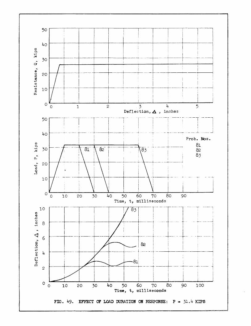
50
I ! n 2. 40 I i -----+-I---rl
:Q ~--+-I ___ f-----+-----+----+---~ - -----1-: - --+--__ 1 ----L-~ "' 30 l! i J
: / I I I !! i I g 20 I --~---r---t- I I
~ --1-----r--1 ---+----IIr--------+---~---- ! ;-~--J-~ ~ 10 I II· I II I : ! : i
I I 1 I :! o 0 1 2 -- 3 4 5
Deflection, ~ , inches
50 i T--l---T---r---I--r -----1- -; - -1 ---1 40 ---~- -- -: --t----r----i~- ->- - - --t -- - - t--- -- ____ L ___-.J
I I : I , Pro b. No s .
I: l- ---l---l 81 C7)
0.
:Q 30
"0'" 20 ~
oS 10
10 20 30 40 60 70 Time, t, milliseconds
~ 10 ----rIi ---
;: --t-~f~~t~~--.S I I "6 4 --------+---+-+---+-
~ 2 1+ L, --+----f-'
I~ o 0 10 20 60 40 50 30 70
Time, t, milliseconds
i 82 83
- -,-
I I !
80 90
- -I ----,
! :
80 90 100
FIG. 49. EFFECT OF LOAD DURATION OK RESPONSE: P:II 31.4 KIPS

I I I , --I-----T i
I 1
T- --I I
! 1 I I ---+------t-----+-- ---+-----+--_. _. J_ .
I iii I I I )
_.3 Deflection, ~ , inches
75 r--T--r-T--1---i--- r -T-; - . 5
60 I ----t---+----11----- - --1-- ---t- ____ ~- - --- ---.l.- __ i , I I '
I I I ' liP ro b . No s • I I I
.~ 45 ..2§+ -l-! 32 -~---~- --- - ~
:: 30 -- -t--r--- -L-~-l --l-_J_- , S : I I I I i l· i
15 11 -T----i\f-\r-l-- +-I~~ - tli--o r ~ J I ~
o 10 20 30 40 50 60 70 80 90
I .... ------
Time, t, milliseconds
8
6
o 0 10 20 30 40 50 60 70 80 90 Time, t, milliseoonds
37 )8 39
100
t...-..~ _____ FI_G-.-50-.-EFFE-_CT_O_F_LOAD __ DURA __ T_I_O_N_OW_RE~B __ PONS __ E_:_P_._5~1_o_3_KIP_~S __ ~J

en a.
..-! ~
... a
.... CD 0 ~ ~ +' en
..-! en CD
a::;
<J
;--I-------T - - ---T---I I I i I ! I :
---+ -- -- -1--- --- --t-- -- ---t- -, I I , i I I i I
75
60
T--'-----l
i
---~---- j--- ! ]--r--------- J -----4--- -+--- ----t ---- -- --- -+ - - J - -
I I
45
30 -r-- -~
15 -
o 0
75
60
45 ----
30
15
I --+--- I I -~ -- -----1 ._--- -+- -
!
I I
1 2 3 Deflection, 6. , inches
-T------- --I-------r---- -,---- ---]-----
i I !
1._ - --- - --t-
37
I --J! --+-___ 1-_ + --- -- + --
; I
! - ----t-
I
!
I
+ I
! t
i I I I
--L--- ~-----L- --- L I ' [ , I Ii; i ' ! --, .. t--i---
I Probe Nos. I
I I , t -- ---- +- ------ - ~
I
31 81
i 37
+ ---
i I o ~ __ ~ ____ ~ ____ ~ __ ~~--__ ~--~----~----~----~----~--~ 10 20 o 70 o 90
Time, t, milliseconds
10 --- r- ----J ----- r 37]--T- -I-~r--~---t- ·1' -- I -1---1-+--
I i --t- -------+---- - -----i-----
8
6 ---- ---t----- ---
! I
4 -- -----1- ----I i I I -------- -- --t--- r---
, 1 I I ! r--t ---t--t--2
o 0 80 50
--T
t --
90 100 Time, t, milliseoonds
FIG. 51. EFFECT 07 LOAD MAGNITUDE Olf RESPOllBE: t • 10 MUJ,TSECONDB p
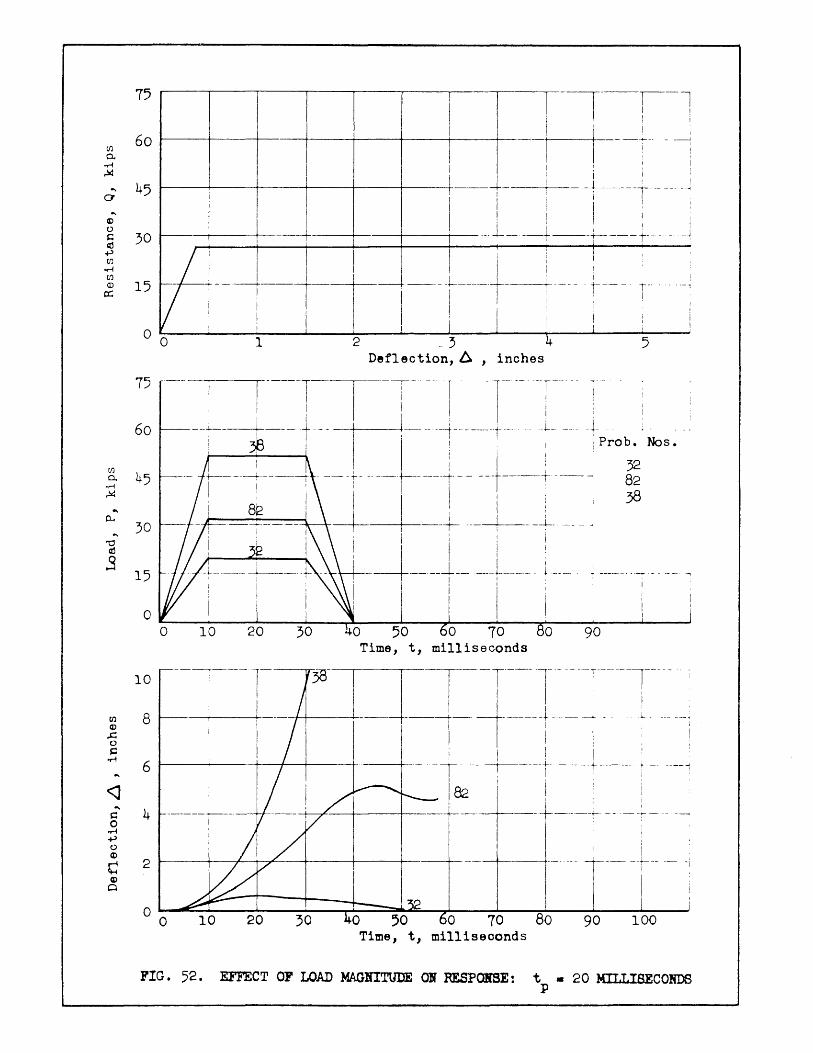
tr.l 0-
..-i
.!Id
."
a ...
CD 0 ~ ~ +' tr.l
..-i tr.l (l)
a:
tr.l a. .~
~ .. 0...
."
'0 d
.9
rn CD
..c:: 0 s:::
..-i
<J ."
s::: 0
..-i +' 0 CD
C CD
Q
75
60
II-i~l
I h----+-45
30
I I I ~ I
~--+------II-----+----+_--+----+I __ -+ I -L--+----- -iii i
l ! :
t-----__ +--!i ---+--, ---.-+---+-----+----+I---.J----~--+----~- ___ j
15 ~- ---1.--1-11 -l.----t-----.l--J" ---- . ~---
I I I , :
.. ·-1 ~_I ! 1 I I Iii
i I' I!]I: l! : ! ,I j I
00 1 2 .. 3 4 5 Deflection, 6 , inches
75 ---i-r---I-TT- --I--r--- -r--I ,I I I
60
45
30
15
-~--;---- t ---nL-- -:----;-~- -- pro~ ~s. -- t-, ----;----: ---r- ---I' -------i-- ----r----+ --~ 82
· ---l-t---L-l- --1--__ ~ ,a
iii I ----j--.---1--- -----!------.-. i --- ~ -----.. -·-r - - .-- .-,
i I I i
I I I
70 o 90 Time, t, milliseconds
38-]=ri--r---T--T------r --10 --1-----)-
8 I I I
I 1---, I I i
82 I I I j
-+---,~--+------+---+---- --+--.--~----~--- -~
Ii • ------T-- t--'
6 I
I 4 ------~--. -
I
2
o 0 10 20 30 o 70 80 90 Time, t, milliseoonds
FIG. 52. EFFECT OF LOAD MAGNITUDE ON RESPOlfBE: t • 20 MU·T,ISECONDS p

.... a
CIJ 0.
oM ..!4
.... 0..
.... "0 ~
oS
til Q)
.c o s:: ~
.... s:: o ~
~ o Q)
C Q)
Cl
~~~~I-~I~~~I~~I~-~----r---~ I I! 1
60.------+---t---i--+-------+----r-I--Li i' ~ I I i I I .
45 ~-_+'--+l--l+___--+---____t__--lt__---L---L-- -1-. - i - ---~
i I I i l ' ! I •
! '1 I i 30 f--. I I iii -- [ ---t----+--- --- - r
15 hLL-J------~-LL--j-~----i-- --~ Vi! I 1 i : :
o 0 1 2 ~ ./ 4 5
Defleotion, 6 , inches
75 ---r --l----r--r--l-- ---I---l--i 60 I -+- ----1 --- -+---~- - -+ - ------+ --- -----+- - - -~
I ! 3 I I: ; Pro b. Nos.
33 45 83
39
30
15
0
-+ -- ----J- -- ----L --I I I I
, I -+--1--I
50 o 90 Time, t, milliseconds
10 ----r- - 8-3-1-----1------I[ I I
8 --- 1---+------+---+-------+ i ----t: .--. --11
---
I I!
6 -----+------+----1--t- ------1-- -- --+----- --i- --- ---- L ---
4 L: --+--.~----+-----l---~- ----1-- I I 2 ~--+----.;.-+-~__+________1-__+_I-- ---
- - 4-I
i 1 I ,
I : ---+------t----- --t-- -
! [
I ---~- ------ -+-
I I ~--~--~---T----~~33
o 0 10 20 30 50 70 80 90 100 Time, t, milliseoonds
FIG. 53. EFFECT OF LOAD MAGNITUDE ON RESPONSE: t a 50 MILLISECONDS :p

eft a.
:Q ..
a .. • 0 ~ , f1l ~
en 4)
a::
~
40
;0
I 20
/ 10
V o " u
50 I
I
I I
1 2 3 4 Deflection,~ , inohes
I ! r--TI 40~--~----+----+---~--~----~--~--~1----+----L--~
I I I Probe Nos. ~ ~ ___ ~_--+ ___ +--_-+-____ -4-__ ~>-----_+ I : 1
:~ 30 !' I: I ~ -0'" 20 r--;::::+=::::;\== ]1 :;:;:::=\2::;:::=::+==:::::::~\~- ~ 3 i i .s \ \ I I
\ \ \ I r---1---1------,------10
o a 60 80 40 50 70 90 10 20 30 Time, t, milliseconds
10 C1.l 4)
.c 0 (:;: 8 -rl
.q 6 ..
(:;:
0 -~ +' 0 4 co r
T--1--I------[ - ;-- f-- i 1
!
t I i
I I---·--~-+---i
I I I
---t- I I! I
!
i I
~ Cl)
0 2
- L--::::--- 3
I ~ ,,- -.....::::::-.. 2
o 0 10 20 :;0 40 50 60 -(U 80 90 100 Time, t, milliseoonds
FIG. 54. IL.LIAC PROBLEM lIOS. 1, 2, 3'
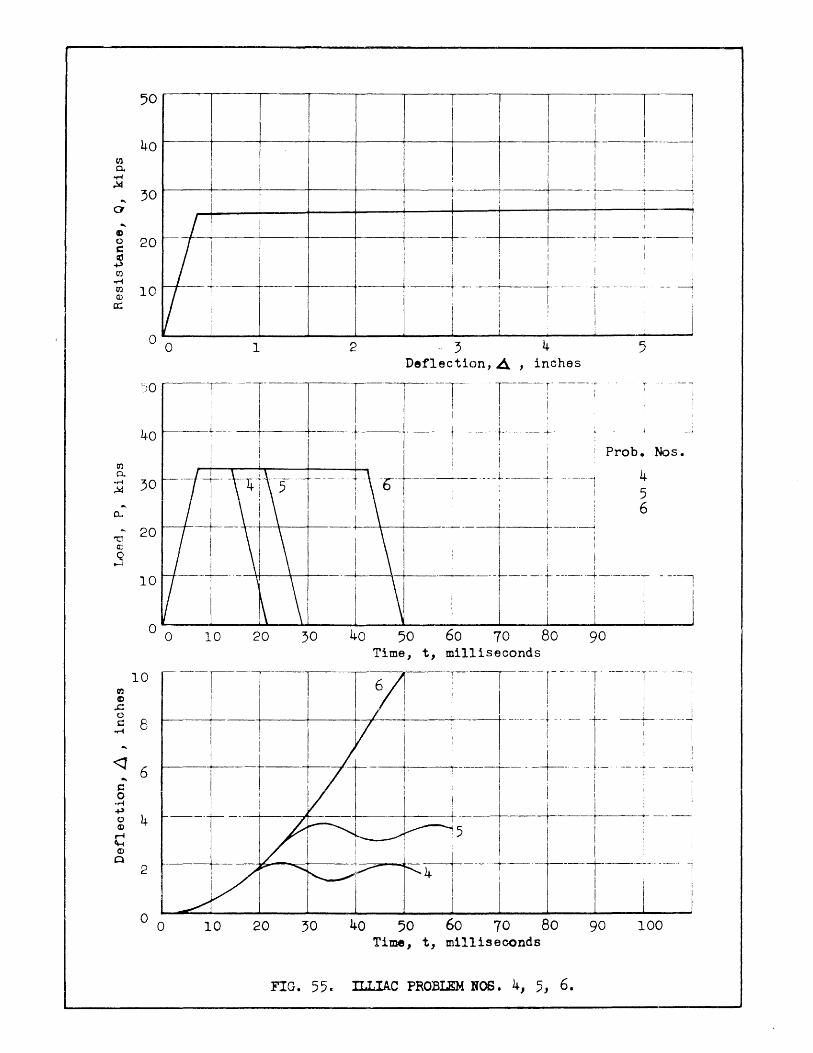
50
40 til 0.. ~
~
"" 30
0
"" I)
0 20 s:: $ 0') ~ 0') 10 CD
0::;
0
'SO
40
l ! !
! r-----l i ,I i i! I ! ! I : I
~--4il---:....!--+--~----+------+-TI ' I' t------;-~I ; I 1 I
~!--4-T--+-! -~---+---+---+~--+-+----L-~!
0
I I 4- I I ! : i . I i I I ---+ !! I -l-l-- l-~ 1----+-1--;1--- ~--p: --I
1 2 3 4 Deflection,~ , inches
5
r 1 ;---1IIT'-T---T . r--r ----I
i ' I I I ' ~-l---- I I' ---+ u._._--+ ____ +_. ----+.-
I, : I : I
! I ! i ! i Pro b • No s •
. ~ 30 ----r-+----~---.....----+---------·---++--b+--~---L-+ -----1 4
10[---r-1i- 'i'\ \\1 -'-+-1 \ --i--I ---t---i----T ... ----I ~ I Ii; j
. j ! . I I i
° 0 10 20 30 40 50 60 70 80 90 Time, t, milliseconds
10 (Il I)
..c 0 s:: 8 ~
<J ... 6
s:: 0 .~
~ 0 4 ~
C ~
0 2
o 0 10 20 30 40 50 60 70 80 90 100 Time, t, milliseconds
FIG. 55 c ILLIAC PROBLEM NOS. 4, 5, 6.

75 T ---1-- ---T----·T--· ---I I I I ! ! :
60 t----+----~--+----t-----+----+I-----r----!-- ---r---~ --1 45 ~--+I--+-----+---+-----+---t-+-- t-- L . '
t I ; ! i
;0 1----+---+--- --+-._--+--- ---I---t--- - -~ - -- t - ----- -f -
... a
15 if1----t-------t--+- J · o 0 1 2 :3 4
.+- -_.- -
1
5 Deflec tion, 6. , inches
75
60
C/)
45 0. .,-4
~
... 0...
.... 30 '0 ~
S 15
I --T---T I --r n r---- r -- -. I I I i I I
-----+---+----- ---- --i-----J--- -- --i------+ -- ---
i ' 9-L- __ J--- _ __, ___ , prOb~ Nos.
i I I 9 I I i I I I I :
--+-+-·~--+-----+---~+----I- --. - +-._- --+- -- . , I I
i I I
t-----l -----0
o 90 Time, t, milliseconds --r---·--i---r- ---T ------
i I --I--r---t-----t I :-' ___ + I __ ~___ j ___ ~ ___ -;_ _ ~
I--l-J---t- -- :--- .-~ I I I i
------- --- r------I
10 -----r-------r-- 9
tI) 8 W-CD ..c::
I 0 C
...-l 6
<J ... 4 c
0 ...-l ~ 0 CD
C 2 Q)
0
o 0 10 20 30
.--- -,
80 o o 70 90 100 Time, t, milliseoonds
FlIl. 56. ILLIAC PROBLEM NOB. 7, 8, 9.

50
40 til 0.
I ...-I .!.4
... 30 a
... / a)
0 20 ~
'" ---l---r +l CJ)
...-I {1) 10 Q)
a:: , ,
I 1
o 0 1
, I I
: i ! I
--,--- ·------+---+----r--1 I I I I
J I ! iii -t---- i t----+---~- -J i' j- ! ! I :
ii, 2 -- 3 4 5
Deflection,~ , inohes
50
40
til 0.
oM 30 .!.4 .. 0..
... 20 "0
'" S 10
a 0 10 20 30 40 50 60 70 80 90
en CD .c o
10
~ 8
<1 6 .. ~ o
oM +l
g 4 r-4 ~ (1)
o
o 0 10 20 30
FIG. 57.
Time, t, milliseconds
40 50 60 70 80 90 100 Time, t, milliseconds
ILLIAC PROBLEM HOS. 10, 11, 12.

.... a
o 0
I ii-l---n __ -+-__ --+-__ +-_-+-1 ---L-L-------t-----l-- ------J
I I iii : I
iii ! I i --+---4-----+--+-----+-----1 ---1-- --- -t-- -1-------+---l
i : I I i .i
t---+----+------+----+-----t---t------+------~- - -- 1------t------~-~ il' I ' - i
: I : I : : --- --------t---+--------+I---+!----i--~+---T -.-. j ---;-~ ; ! i I I Ii! : i I
1 ' 2 3 4 5 Def1ection,~ , inohes
50
40
til a.
'M 30 ~
"" 0...
... 20 "0 ~
oS 10
--1----1-1=--r-T --l- -T .. ---t---l------- --~---~----1---+- . Iii I : :1 i ! Prob. Nos.
,....-+----.--...,....y---+---__ I _ Iii ; 13 ----- -- ~-- ---r-----+ --- ----L --- -t- ----1 I 15 I I : : I 14 I Ii: 15
-+----+1- --t-- 1--1-- ----~ I I I I
I I : i --t---~---_+! ----- :-----i------ -:---
I I
I I
o 0 10 20 30 40 50 60 70 80 90 Time, t, milliseconds
10
<1 6 .... t: 0
'M +' 0 4 Q)
c: Q)
Q
2
o 0 10 20 ;0 40 50 60 70 80 90 100 Time, t, milliseconds
FIG. 58. ILLIAC P~OBLEM NOS. 13, 14, 15.

G') 0.
or'! ,.!oC
.... a
.... CD 0 t: .s C/)
or'! C/)
~ a:
fIJ 0.
or'! ~
.... 0...
.... "0 ~ .s
fIJ C>
..c: 0 s::
or'!
<1 ..... ....
s:: 0
or'! ~ 0 ~
t:: ~
Cl
50
40
I 1
I I I
I I
30
20
10
r I
I
/ ~-
! I I I
1
1 V ----4- I
I I
I
I I I ! !
o 0 1 2 4 5 Deflection,~ , inches
50
40
i-T---r---r---T----- r-' ~-+--t_____+__+-+---+____+____+_I ---+-1 _ t L---_L ____ J
30
20
10
I I I
j I I I I Probe Nos.
-+---+---- -- -- - --1--t-------i l6 I I I i l7
++---+---1f-----+-1 - ! i
I I I +--L--r
10 20 30 40 50 60 70 80 90 Time, t, milliseconds
10 I -- --l
8
6
I I
-. -- ----_._. ~----1 /; ..."..----.... -----.. il ~ ~-".. "
j
4 ~ / I j
2 / ./
o 0 10 20 30 40 50 60 70 80 Time, t, milliseconds
rIG. 59. lLLIAC PROmD Ice. 16, 17.
i 90 100
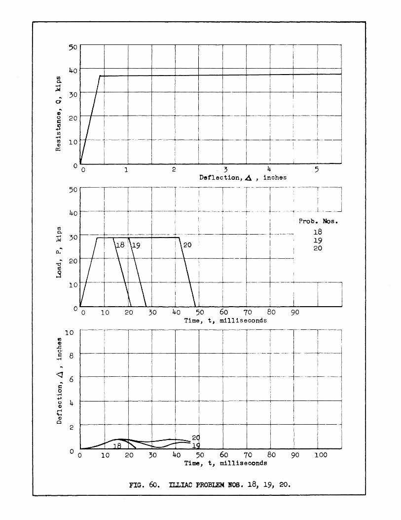
Ul 0.
;Q ...
a ...
c 0 c ~ tf)
orl OJ ID
a::
CIJ 0.
..-4 ;4
... 0...
... -0 ~
.s
In C)
..c: o-s::
..-4
<J ...
s:: 0
• ...-1 .., 0 ~ r-I fH ~
0
50
40
f I i :
30
20
10
/1 I I I
--~--+--t--! I I +- i ; I ~ - - -t---t--r- :
I ! I I o 0 1 2 3 4 5
Deflection, ~ , inches
50
40
30
20
10
o 0 10 20 30 40 50 60 70 80 90 Time, t, milliseconds
10
8
6
4
2
r- 1
-T_IJ~l I I I
f----
~--H I I I
i -- --- -+--- -4---t- ---I I ! I ! I I
I
I !--r i I
l -
~ .......... '8 .... ,~ ~ ~2~
l~ o 0 10 20 30 40 50 60 70 80 90 100
Time, t, milliseconds
FIG. 60. ILLIAC PROBLEM BOS. 1.8, 19, 20.
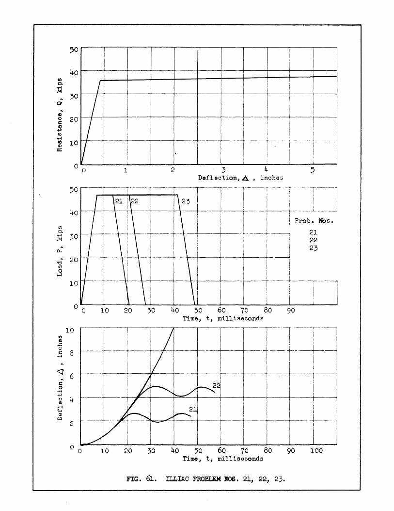
50
40
/ I + /1 .l---t I i I I I I
I I ; I I I
I I I I
... C> g 20 / I ! I
, i lO~ I I I I· I I
o 0 1 2 '. 3
1 I I I I
1---+1 u ~--1---1--1
Ct:l 0.
50
40
:.Q 30 ...
0...
'0'" 20 ~ .s
10
4 5 Deflection,~ , inches --4-----r-- ---. T'- ----i ----i-----l
I ' I I I
1 23 I:, I i I - I ! I I I -i--- "-l---r'--r~:';'~~-~s-~J
-T---+ -J-+---L--.-+~ 21 I ' 1 I : I 22
I I I i I 23
+-+----4----+-. -----+1-- -t-------" I iii I I I
-t---+--T----i , ' I
I
o 0 10 20 30 40 50 60 70 80 90 Time, t, milliseconds
10
2 I
--i
I
i I
I I I-I
10 20 30 40 50 60 70 80 90 100 Time, t, milliseconds
FIG .. 61. ILLIAC nOBLEM KOS. 2.1, 22, 23.

til 0.
orl ~
... CI
... CD 0 c ~ ~ til
orl til ([)
g::
(/)
a. oM ~
... p...
... '0 ~
.9
til ([)
..c:= 0 s::
orl
<J ....
s:: 0
orl +' 0 CD
C CD
CI
75
60
45
30
15
0
75
60
45
30
15
0
10
8
6
4
2
In ! I .----+---+---+---+---+----+---+-----+---+-~--~
I I i I
~-~--+I--~-~--~--~I,--~i--~--l--~-~ II ' i I·
ii' / ; I I I I I
~+-+--Il _.-+-! --+------+---+---1---I-ri--r-~
-1---,---r [I '----r-----t-·~i----- -i--
0
1 I 'I 11 I I : \' I r ii, i
1 234 Deflection, 6 , inches
5
.. -.--- -l -r---1--1--r----r -i ----r---- -i I 1 I I,
t----t---+---'~_t------~ ---t---~- ----;- ----1--- ----L- - - 1- - -..
r iii : , : ! Pro b. Nos.
I _ --t---- -t----f-- ---+ ---- -t--- T ----, 24
i i : ! I
-+----+-1 _ l---i------l-----.~ I I I i
I I i I' i I ; I . ! -r ---r1--i--t-j"-
10 Time, t, milliseconds
---,-----,--·---·--1- ·-----T .. ----- --T----- ~
i ! I I I I I I I I I ' ,
i I r--t----1----:-; i : : 1 i ' -t-----1----- -1- -----+-- -- -~.-- . ---t- ----:-
iii iii i - -t---- I -+---+--i-L ___ . ______ ~
~--t---t---+----+---+----~----t --~--a 0 10 20 30 50 90 100
Time, t, milliseoonds
FIG. 62. ILLIAC PROBLEM NO. 24.

en 0.. . ..-; ~
.... a
.... CI 0 s:: ~ +' til ..... C'Il CD
a::
50
40
30
20
10
! In t----t---+-----+----+-----+----+----
I- +--r---~
/1 I I I : I
/ I
I. ' i -1-11--- i !
; I i I t----+---+----+----+--+----+----+--- _--L--_-+- I -r-~
/
I : i : I ' II I I I I I I I I I' I : i
V T, -------;-1: ---r--------+----+-I-t---t---~----;-~
I 1 I 1 J o 0 1 2 -- 3 4 5
Deflection, ~ , inches
50 --- ----r
~ ~---+-----~----t ___ i _ ___ -1-- _ ; ___ ~ ____ ~ Prob~5 ~s. :Q 30 I I I 6
'0"' 20 m S
10 C'Il CD
..c::: 0 c 8 .....
<l 6 "' ~
0 oM +' 0 4 CD
,..-4 ~
CD 0
2
26 27 I I . : I 2 I i I I ! 27 -+---+-------r------+------t-------< -
I I I
I I :
--+-- ----~--- ---i----- ----1 ----I : Ii: I : I I I I I I I I I I
10 20 40 50 60 70 80 90 Time} t; milliseconds
[---r---] -r---r-. iT----T---]----l. --T---l. 1--1 ~-]----i---r- 1-- - t- -:---~
~--+:--+-+-- --- --+-+-----+- -- -~--- :-~ I ! I I I 'I I
-+--! I 1 --1--- -l- : -+----+--~ -r- I ' I I I •
i i t 1 : : ---t---------r---- ----i----- 1
o 0 10 20 30 40 50 60 70 80 90 100 Time, t, milliseconds
FIG. 63. ILLIAC PROELEM NOS. 25, 26, 27.

I 1 T--T I I
I I I i I I I ----1-- -T--------' i j I I
50
40
; /!I iii I I i I ~ i I' I I 30 ~--+----+--___111----+--------+----+-----+·-- ------1---- I t-- I-~ a / i, II I L' I ~ ; i ~ I I I I g 20 ---I~---+----+-- ----f----- ----+------+------+------.--, ~ r I I I!: 1 : i
i 10 --+---t---+----ti-1---t~--t-- :----T -~~ I I i I I' I I
o 0 1 2 4 5 Deflection, ~ , inches
50 I~-r-I-J\-l~-T----i- -r --r--- -; ----; ---r
40 ~~/+---\~-t~~--+I-~--+---+- --+1--- - --t - ~- -- ~ i I I: i I Pro b. No s • I I I I I t-- !-t--T-:-~-t---:---;----i ~~
... 0...
~-~--- I --+-----.,----+-----1------'
] 20 __ J____ --1 i ---1-- '----L---,----~ 10 I I: I I
<1 ...
s::: o
o 0
6
:;; I o 4 (l)
~ (l)
Q
2
o 0
10
10
20
20
I ! I I I I I I
30 40 50 60 70 80 90 Time, t, milliseconds
~ -~---r-! -----r- -: -+-----+--~-+-----+-- --- i-- ~ --+ -- -1
I I : I - --+-- -i--- -- -t- -----1 I I I I I I I i
-----..~'C.--__+__-+--+--~ i : I
~I i i
I I ----- -------f-------1
I i I
30 40 50 60 70 80 90 100 Time, t, milliseconds
FIG .. 64. ILLIAC PROBLEM NOS. 28, 29.

75
tf.I 60
0-.,-j
~
"" 45 a ...
CD 0 s:: 30 '" ~ tf.I
.,-j
tf.I (l) 15 a:
0
75
60
45
... 0...
30
15
0
10
8
6
4
2
0
II I
I, '!!
1----+-+-------+------+--+----+------1--- --+---- ----+---- -+-- -- --~ I ! I I
0
0
--
0
-~ I
I iii
----+----+--~--+--__+I--~~---t--- L_ I I I I I
I
10
I 1 1
20
--r~~'-
--rl
10 20
30
I I I I
! j : !
234 Deflection, ~ , inohes
Time, t, milliseconds
5
I
---t---
i !
-- -----t------1
-4-------i-----!---+----+-- -+----+---.. ---- ~ .. -----1
-------r ----- - -_. ~
30 o 50 o 70 80 90 100 Time, t, milliseoonds
FlO. 65. ILLIAC PROBLDl 10. 30.
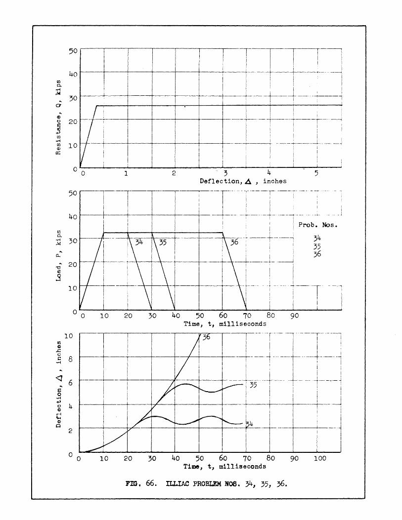
Ul 0. ~
~
"' a
"' G)
0 s:: .s Cf)
~
til Q)
a::
Cf)
0. oM ~
'" 0...
.. '0 co .s
50
40 I
30
20 ~_/
10 -H I i !
o 0 1
50
40
30
20
10
o 0 10 20 :;0
o 0 10 20 :;0
I TIl Ii i: ,I I J~- I ~-~-I Iii I • I I Ii' . i
! . I I I ---t --+------t -"" --~--"-1 . I I l j
I I I i , , I I --r-"--t---T----r---~
~--+ i~---~----~d-_-~ ' I I
I I i I I i 1 ii' ! : i I : "'
2 :; 4 5 Deflection, ~ , inches
40 50 60 70 80 90 Time, t, milliseconds
40 50 60 70 80 Time, t, milliseconds
90 100
Fm. 66 . ILLIAC PROBLEM NOB. 34 J 35, 36.

~ 0. ~ ~
.... 0
.... e 0 s:: ~ ttl ~ OJ CD
a::
~ CD ..c C)
c ~ .. --"'" .. s:: 0 ~ ..., 0 CD
~ CD
0
50
40
:;0
/ 20
/ 10
/ °0"
I
1 2
1\40 1\41 \\
20 30 40
D I I
I l j I I ! --
!
i- l I
'11] I I
I ~---l-- 'i
I I :; 4 5
Deflection, A , inohes
50 Time, t, milliseconds
t----+----+-----+----4------+-----+--4-----+-----~~~i~ 10
8
ti--1 I I
I
6
4 I
2 ~--~--+_--+_--~--+_--4_--~--~---~--~--~
42 41
-----o 0 10 20 '0 40 50 60 70 80 90 100 Time, t, milliseconds
P'IG. 67. ILLlAC PROBLEM lOS. 40, 41, 42 •

Ul a. ~
~
40
... ;0 CI
fIJ" / j 20~/~+---~--~---+--~----~--~
~ I I ! i .-.-t-----r--~
~ 10V I 1
I I
I I I i o 0 1 2 ; 4 5
Deflection, ~ , inohes
50 IT, - -1---11---1-1 40 ~+--I----+--~--+-----+---- ---t----~-__ -L __ ._J
I I I' I Probe Nos. I ! ---1-4;!--t---l' ~~
I I 45 -+---+-4----+------f----J
~-+----+----+---+-+--i-i-l-.; 20
cx3
.s 10
10 w:I C)
.c 0 s:: 8 ~
...... "-.l .. 6
s:: 0 ..... ~ 0 4 ~
C a>
0 2
o 0
10 20
I
_/ V
10 20
30 40 50 60 70 80 90 Ti~e, t, milliseconds
/ 45
----f~ ! i I
) v--..... "--V-~441 T~
/ / ~ - ~ ~ ~3
;0 40 50 60 70 80 Time, t, milliseconds
.~ I
90 100
FIG. 68. ILLIAC PROBLEM HOS. 43, 44, 45.
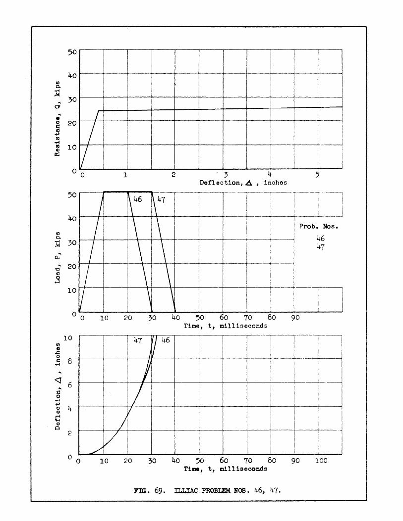
40 m 0.
...-4 ,J.(
.. '30 o ... f
J..----I--+---+---+---+---+---+--+--+---+---+--~
~ 20 / i I I
!lO~/~~~-~~~-~~-~-~l--1
0'
50
40
10
<l 6 .. s:: o
...-4 .., g 4 ~ \-4 «>
o 1 2 3 4 5 Deflection,~ , inohes
10 20 30 40 50 60 70 80 90 Time, t, milliseconds
47 y46 1---'-' ----t---t-J t--t----~ -- ! I
! I
I I I I I J
~
21 =r I I I I I I I
o 0 10 20 30 40 50 60 70 80 90
1
I 100
Time, t, milliseconds
Fm. 69. ILLIAC ,PROBU!M NOS. 46, 47.

en 0.
~ ...
a ...
G)
0 c Q,'I
+3 U)
..-1 CI) II)
0::
CI)
0. • ..-i
~
... 0..
... "'0 ~
oS
en G)
.J:: 0 s::
..-1
<1 ...
s:: 0
• ..-i +3 0 II)
~ ~ II)
Q
50
40
30
20
10
0
50
40
30
20
10
10
8
6
4
2
0
i" I I I I : I : I I: I I ;
---- +1' ------I------~-- --+l---------i---t -- j- -- T --~ I I I I I I I I i j iii I
i 2
10 20 30 40
I 50 - --r- ---,--,---
-3 4 5 Deflection,~ , inches
50
-- -+ -I
I ; -. ------ -+- ----- -~
I ,
i I ---1------+ - _____ J
I I i
T
Probe Nos.
48 49 50
-1---- -r--- --7 4- ---- --- - -, I
I
60 70 80 90 Time, t, milliseconds
--- -r --------r- -- ---l I I '
- I
91
--- i---l----1-*----+ ------t---------i-- - ------
I : I
I I ,
~--+----+----+ i I I
- -----1------
I ! I ; , I ----4-- --1-- --- ---~- --- - -+- - - - ---- i --- -----i
I I I
! I I I
~+----+------+----+------~-----~--~ ---1
--------+--- -- + I I
1 ! I I -,-----
iii i i •
I---+-------,+---+----+---+-i---t ---- ---1--1--- ~
! I I I
o 0 10 20 3D 40 50 60 70 80 90 100 Time, t, milliseconds
FIG. 70. ILLIAC PROBLEM NOS. 48, 49, 50.
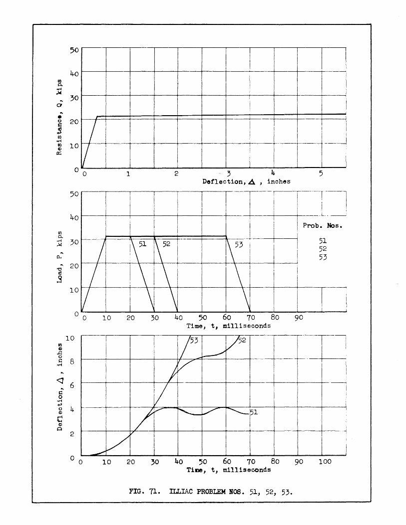
CD 0. ~
~
.... a
... • 0 s: ~ U) ~
CQ co a:
C1J a. .~
~
.... 0..
'" "0 ~
S
CD ~
..c 0 t: ~
<3 ....
t: 0 ~
~ 0 ~
C ~
0
50
40
30
--
-L-I
I
20
10 / I 1
I i I
V 1-~ i I
o 0 4 5 1 2 Deflection,~ , inohes
50
40
30
I r--r---r---T------T----l
I I ; , I I :
I __ ~ _____ L--"
I ~ Prob. Nos.
I 1\51 \52 --+-- 51 \53 I 52 1 I ! 53
20
10 / \ \ '\ I i I
I --
V \ \ \ I I I I
o 0 60 80 40 50 90 70 10 20 30 Time, t, milliseconds
10
8
6
/53_ /52 -~ ~ --r----.-
~-1_1 J V --'----
I i
4 I ~ ,/' ~~ ~ ~l I
/ I
2 +-V/ -'" I
o 0 10 20 30 40 50 60 70 80 Time, t, milliseconds
FIG. 71. ILLIAC PROBLEM lOB. 5J., 52, 5:3.
90 100

50 I-t-! ~,i II' I
'
i I I 40 t----+---+----+---+----+---_+__ ---+--1 ---+----1---1
~ II I I I I I ..!14 I I i I ... 30 ~--+----+----+-----+---+----+ I! --;---l
a
... / I I i I g 20 t---+----+----+---t------+----t---+-----+---t- I --+---1
~ Iii I ! !
] 10 'IH--r--l
C1) 0-
o 0
50
40t---+--
1
1 1 I ! \ I J 2 4 5
Deflection, ~ , inohes
I -TT---iim-~--l +-----+-------1--- I +- _____ 1 _____ J
I I
I 1
--+--------fl~-t ---~ ----l I II I I I
] 30
Probe Nos.
57 58
10
10
2
i I I'
: I •
10 20 30 40 50 60 70 80 90 Time, t, milliseconds
59
1/ o 0 10 20 30 40 50 60 70 80 90 100
Time, t, milliseconds
FID. 72. ILLIAC PROBLEM NOB. 57, 58, 59.

50 =+1 Il~-Tl 40 -- ----+---+---+----+----+----+-- -----+-1 -----t------r-]
til I I I i 0. I, ! : 1
:Q I I --+----+----L--a 30 I I I I I I ~ r 1 I I
CD ! I 'I
g 20 I I 'I : [ I I ~ I I I I I
~ 10~~+~~~-+-------+----+·--+~_+-f-----~~~~~- , ex:: 1 I ! I I I I ! II
i \ 1 1 I ; ! j
tI)
0.
o 0 1 2 3 4 5 Deflection,~ , inches
50 ----r-l-r-~r=r-T r--- -~~- !-T-~i
40 --+------r------+-- I - - -~ ----- -+------ ~ -- -- -_i U_H J 'I : I I I: I I P b No I
I I I , I ro. s. I I 1
I I L I : b"2---. ----t-- -----1
i : ! ~ 30 60
61 62 ....
0-.
rn CD
..c 0 ~
...-1
<1 ....
c 0
.r-i ~ 0 a>
,.-i \-t a>
0
10
o 0
10
8
6
t-----l.----~ I I
~t- - ----~+- --T ----, I
10 20 30 40 50 60 70 80 90 Time, t, milliseconds
--t---+J~ 2
i -~t-~-~-
61 ~r-~-T-T---l--~--~T--'
·--I--V------+-+----~t-~ --- I ~- ----+--~ ! -~+~~- ;-~-~~---~--~-j~--j
I 4 -i--- I 'I 'I' i ~-=~- ~ - I ~
i I
I 2
o 0 10 20 30 40 50 60 70 80 90 100 Time, t, milliseconds
FIG. 73. ILLIAC PROBLEM HOS. fIJ, 61, 62.

:: I [ I
~ ~ t----~i ---+--+-----+----+--+11
- I I_t-l. __ ~I-J _./0 I ,---t--t- 1 I ,
c: I : 1 I
g 20 I --~-·t- \ -+-11
---:
.s 1 I: 1
0) I I ! i I I I
~ 10 i- 1 ---1----+--·- -~ a:: I I I i
0)
0.
o 0
50
40
:Q 30
1 2 4 5 Deflection,~ , inohes
-I ----IT--T- --) - r-- -r- i +----+-----+---+-----+I--H---i---i---- _L __ ~
I I I I I Probe Nos.
p...---+---+---.--t--___ -. -----+--=~---\ ---- -L I I 63 65 i I I 64
i I I 65 ~~~ ---~~~~-+----+---~~-~I--__t-~
] .. 20 I 1 I
.s 1 0 t--~-- --I I I
o 0 10
10
2
o 0 10
20 30
20 30
40 50 60 70 80 Time, t, milliseoonds
40 50 60 70 80 Time, t, milliseconds
FIG. 74. ILLIAC PROBLEM NOS. 63, 64, 65.
90
!
i
----1 90 100

50 --'----r--- --- ------r-
! I I I ! I i I +----t------i---t--- .. I
- j... - - -
I -~ -----1---- --_______ ~ ': 1
I I I, I !, r I
i I I : ;0 l------+:---4+: ---+---t---t---~: ----1"-- -----~-------t-----I--iii J : .
50
40
en 0. ;0 :J .. 0.. .. ~ .,
20
.s 10
Defleotion,~, inches 1---- 1-- -----r-- --- T- --,- - 1 T
I I i I I I I '
-~----J- -i------- l. --, I
I I I
I
.- - j
- --+---I
-+- -- --+ I
I
t
- -- + -.j.
4
- -~ -
-T----
i 5
I
I
I ---~
t Probo Nos.
t - -- - 1
I -- --- +
69 70 71
I o ~V ____ ~ __ ~ ____ ~ ____ L_ __ ~I ____ ~I ____ ~ ____ ~ __ ~ ________ ~
o 10 20;0 ~~O 50 60 70 80 90
Time, t, milliseconds r -
10 ----1--- ---r-----l----- r- 7i---; -'r
I I
I I -
I
-- -+ I
I -
I
I '
--_ - - - - _1 _ _ --1 8 , I '
! I! I I I I
--------+i - --~' -----r--- --I '
I -----t-
6 10
4 t- -!
-i--
,-
---+ - - ---+-
I -t
2 ! I
---- +-----+- --i I
! I I
o ;0 40 60 o 50 10 20 70
I
80 90 100
Time, t, milliseconds
FIG. 75. ILLIAC PROBLEM KOS. 69, 70, 71.

50
40 III 0.
lJ 30 --.
CI
... I) 20 0 s: ., ~ III
"" 10 Ie CD
a::
0
50
40
30
20
10
0
10
8
6
4
2
0
I I I t-------1--.---,.----+---+---ri--l I I
~~i--~~--~-~!---J---~i--~I'--+---~I ~ I i I! Ii Ii i I I
I I I
i I I I : : I ! ! I j
/ ----t----l--l--, I I
! I !
I , I I I t--+---+----+-
I ----11
------+--! ------t---t--I
' : I i I : : \1 I I I i I
I
I I 0 1 4 5
De!1eotion,~, inches
i --T ~ ---;~ --T--T---T--r------;--T------,' .----+-1 ----I---+~-----L---~-----+---~----t_ I_~
'II i ; : i ! I Prob o Mos.
0
1 1
~---T----~--~----~--~ f 84 85 86 : I
------+-----< I
. , I I ! 1
~--+___--J---r---I 1 I I I I 1
I : I I 10 20 ,0 40 50 60 70 80 90
Time, t, milliseconds TI~ ------1--!-----T;----T- ---1'-(---1 i,l I:' I· 1 ,5 I, : ' I'
.----+----+----+-11
---- ---1------:-- --r------+I---T-----r---1 : I· I I .
t--_-+-__ +---__ -+-i -I--+-------t---- -1------~-L-----+----L-~
~.-_,_I_ iii I I
t-----+----+------~~--r -~--~---~--~
I i I I
t------+--~C-.--+-----+---+--t_-----+---+---+--+----l I i
0 ;0 40 50 60 70 80 90 100
Time, t, milliseconds
FIG. 76. ILLIAC PROBLEM NOS. 84, 85, 86.

CI) 0.
oM ~
'" a
'" G)
0 ~
$ tf)
oM Dl tD
c::
tr.l 0. .~
~
'" 0...
--"0 ~
3
CI)
tD ..c 0 c
oM
<q '" c
0 .~
+> 0 Q)
rf tt-1 (!)
0
50
40
30 I
I
20
/ 10
/ o 0 1 2
---I I
I ! I
I : , !
1 I - -+-------,
j I
i J ! I I . i I
! I I---t--~ I I I I lUI I I
: I I I I H---I ,--r---r-i :z .J 4
Deflection,~ , inohes 5
5°111 40j-i-----l-
i----T- --1----- --T---l I I ! i ---+-----4----.+-_ ~----+ __ --- _____ J. -- ___ J
30
20
10
o 0
, I I
: I j I Probe Nos.
~===:t====t====t===-==t:===::j -----1-- +-----~ 87 I 89: I ! 88
10
I Ii: . 89 I I : i :
---+---\---+---1t---+--- I -r-- ---L ----4- __ ---J
,--\---+----4----+
1-4+- -~---f- ---f---T ----; 20 30 40 50 60 70 80 90
Time, t, mil1iseoonds
10 ,- I I
T 8
~ 6
4 I 2
o a 10 20 30 40 50 60 70 80 90 100 Time, t, milliseconds
FIG. 77. ILLIAC FROBLEM NOS. 87, 88, 89.

c : IJ----+--I --+------+--1 1 ---+----+---1 1 ~I -~ Q. i I i
I
~ 30 J ! .. o
.. c..
.. <J r: o ~ ..., o ~ r-t
~
I
/ I
V o 0 1
',0
~.(i ---r-
30
20
10
0 0 10 20 30
10
8
6
4
I L 1
I I
+-+ 1
!
I
I I I 2 3 4 ,
De!1ection,~, inches r- I
.1 I
I I
I I
-i I I
.--4----j-~u . I 1 Probo )los.
I : 93 I I 94 ; I 95 I I
~--~~--~----~I --~I
40 50 60 10 80 90
Time, t, milliseoonds
~ 2 ~--+---~~+---~~~---~~-r---~---r---r--~ o
o ~~~--~--~--~--~--~--~--~--~--~----o 10 20 30 40 50 60 10 80 90 100
Time, t, milliseconds
FIG. 78. ILLIAC PROBLEM NOS. 93, 94, 95.

NOTE: In Beams Without Compression Reinforcement k'=k
=== =='====--==~:=lTl . d
11
ibi • i
• •
• •
n Ey
CPy = (! - k I ) d "
fy I I
E =-Y Es
Cross Section Strains
ifCI -nkf¥=r=<; = 1/2 k' bdfc kd f ----C-=t\('
2 s S t---, jd=(I-k'l3)d
(I-k' ) d
l 1--___ -1--1 _._- T:::: fq A~, ) "
Stresses
FIG.79 ASSUMED CONDITIONS AT YIELDING
(Fig. ;6 of Her,. 2)
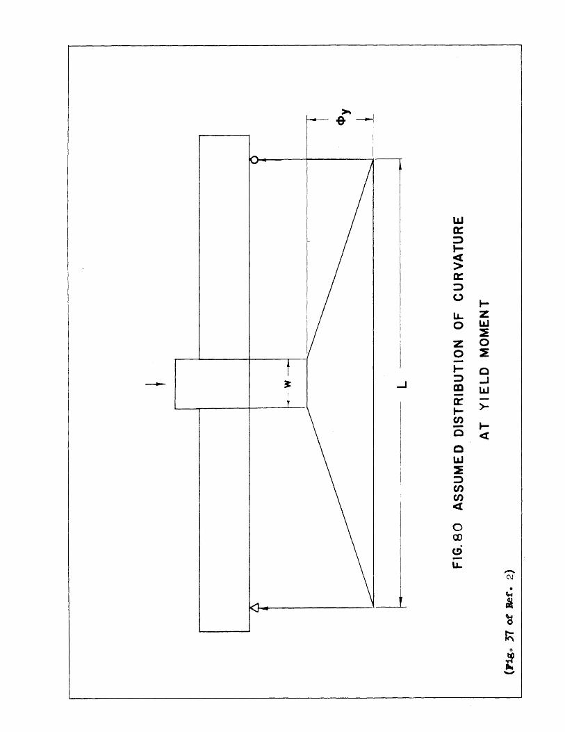
W 0:: ::l I-ct > 0:: ::l (.)
l-LL. Z
L&J 0 ~
z 0 0 ~
l- e ::> ...J -l en UJ -a: >-t-C/) -0 ,..,. -UJ ~ ::> en en ct
0 a:> (!)
LL

2.0
LEGEND 1.8
1.4
- 1.2 "U
(J)
<l: 'I~ >< ..... 1.0
0 E ~
0.8
i 0 Series T I tl Series B
I
------t-- • Inverted I :
I: I
I i I --1- -----t----- J- - ~--- --~-~
1.6
-- ---~ --- --- i--
I
--j-ii' , - .. -._--. ----/-- ·-·-~I~~-LOfll;;·~=--:-F:::~~'~
l--- -- ----L---L-~---_+ I ! I l i
I I I !
I l-r--- r -- - -- ,- r - -:-------t--
o
0.6 --t--
0.4
0.2
I I ' i· -- -- r -1---1 .. . - ,- --
f-I--f--l I
----
o I :
-0.3 -0.2 -0.1 o 0.1 0.2 0.3 0.4
q'=(pfy p't'y)/f~
FIG.81 RELATIONSHIP BETWEEN ql AND fs AT MAXIMUM MOMENT.
PLOT OF NOMINAL fs DIVIDED BY fy VERSUS ql.
(718. 41 of Bet'. 2)

16 Legend
14 • T-Series CI)
OJ l::A 8-Series
.c 0 12 c • !:
~'---
c 10 c a. CI) -----0
~ 8 •
.... c ~ c: 6 0 .... 0 OJ
\4- 4 Q)
T-9 • ~ • •
~ 0 6 •
2
0
-0.2 -0.1 o 0.1 0.2 o. ~) 0.4 0.5
.1 = ( f - 'f I ) / f' q p spy c
FIG.82 DEFLECTION AT MAXIMUM MOMENT '/ERSUS q"
(:rigo 42 of Ret. ~2)

DISTRIBU.r:iON LIST FOR BLfillT &w SHOCK RAND D REPORTS ~{ISED~ 20 Dec 55
ADDRESSEE
Chief of Research a.nd Dev-elopment'J D/ AJ Wa.shir"gtc<c 25 ~ Do C 0
ATTN~ Atomics, Air Defense and Missile Division
Chief of Engineers, D/A, Washingtcn ATrN~
ATTN~
ATTN~
ENGNB ENGEB ENGEL
NO OF CYS
l
""i .1.
l 1
Commanding General, Continental Army C0rI11nand.9 Fto Monroe, Vao 1
President, Board Noo 4, Head~uarters, CONARCs Fto Bliss, Texo 1
Commander-in-Chief, FECOMj APO 500J San Francisco, Calif 0 2 ATTN~ ACofS j J-3
Commandant, Command and General Staff College, Fto Leavenworth, 1 Kans 0 ATTN ~ ALLLS (AB)
Secretary, The Antiaircraft Artillery and Guided Missile School J 1 Fort Bliss, Texas ATTN~ Majo George Lo Alexander, Dept 0 of Tactics and Combined ~1rms
Director J Special Weapons Developme:J.t Offi~e J Headquarters J 1 CONP~C, Fto Bliss j Texas
Commanding General, Research and Engineering CommandJ Army 1 Chemical Center, Mdo ATTN~ Depaty for RW and Non-Toxic Material
Commanding General j Aberdeen Proving Ground~ Aberdeen3 Mdo ~
ATTN~ Direct-or J Ballistics ReSearch Lab
Commanding General, The Engineer Center J Fto Belvoir, Vao 1 ATTN~ Asst Commandant 5 Eng School
Commanding Officer, Engineer Research and Development Lab J 1 Fto Belvoir, Vao ATrN~ Chief, Tech Intelligence Branch
Commanding Officer, Picatin.YJ.Y Arsenal,9 DO~ler} N 03 0 ATTIii~ ORDBB-TK 1
Commanding Officer, Chemical and Radiol.ogical Lab, Army Chemic.al 1 Center, Mdo ATTN~ Tech Library
Commanding Officer~ Transportation Rand D Co~~dJ Fto Eustis, 1 Vao ATTN~ Special Projects Divisi0n
- 1 -

DISTRIBUTION LIST FOR ~ BLAST AND SHOCK R .AlID D REPORTS
ADDRESSEE ARMY NO OF CYS
Director, Technical Documents Center, Evans Signal Lab, 1 Belmar, NoJo
Director, waterways Experiment Station, PoOo Box 631, Vicksburg, 1 Misso ATTN~ Library
Director, Operations Research Office, Johns Hopkins University, 1 7100 Connecticut Avenue, Chevs Chase, MUo, Washington 15, Do Co
Chief of Ordnance, DI A, Washington 25, DoCo ATTN: ORDTX-AR
NAVY
Chief of Naval O]?erations, DIN, Washington 25, DoCo ATrN: OP-56
Chief of Naval Operations, DIN, Washington 25, DoCo ATTN: OP-03EG
Director of Naval Intelligence, DIN, Washington 25, DoCo ATrN~ OP-922V
Chief, Bureau of Ordnance, DIN, Washington 25, DoCo
Chief, Bureau of Aeronautics, DIN, Washington 25, DoCo
Chief, Bureau of Sr~ps, DIN, Washington 25, Do Co ATTN: Code ATTN~ Code
Chief, Bureau of Yards and Docks, DIN, Washington 25, DoCo ATrN: D-4oo ATTN: D-440
348 423
1
2
1
1
1
1
1 1
1 1
Chief of Naval Research, DIN, Washington 25, DoCo ATTN: Code 811 1
Commander-in-Chief, UoSo Pacific Fleet, FPO, San Francisco, Calif 0 1
Commander-in-Chief, UoSo Atlantic Fleet, UoSo Naval Base, 1 Norfolk 11, Vao
Commandant of the Marine Corps, DIN, Washington 25, DoCo 4 ATTN: Code A03H
President, UoSo Naval War College, NeW]?ort,9 RoIo 1
SuperintendentJ DoSo Naval Postgraduate School, Monterey, Calif 0 1
- 2 -

DISTRIBUTTON LIST FOR ~ BLAST AND SHOCK R AND D REPORTS
ADDRESSEE NAVY
Commanding Officer, 00So Naval Schools Command, UoSo Naval Station, Treasure Island, San Francisco, Calif 0
Commanding Officer, UoSo Fleet Training Center J Naval Base J
Norfolk 11, VaG ATTN~ Special Weapons School
Commanding Officer, DoSo Fleet Training Center, Naval Station, San Diego, Gal if 0 ATTN ~ SPWP School
Commanding Officer, Air Development S~uadTon 5, VX-5, UoSo Naval Air Station, Moffett Field, Calif 0
Commanding Officer, UeSo Naval Damage Control Training Center, Naval Base, Philadelphia, Pao ATTN~ ABC Defense Course
Commanding Officer, UoSo Naval Unit, Chemical Corps School, Army Chemical Training Center, Fto McClellan, Alabama
Commander, UoSo Naval Ordnance Laboratory, wr~te Oak, Silver Spring 19, Maryland ATTN~ EE
Eli R
Commander, U.So Naval Ordnance Test Station, Inyokern, China Lake, Calif.
Officer-in-Charge, UoSo Naval Civil Engineering Research and Evaluation Laboratory, Uo So Naval Construction Bno Center, Port Hueneme, Calif 0 ATTN~ Code 753
Director, UoSo Naval Research Lab, washington 25, DoCo
Commanding Officer, and Director, U080 Navy Electronics Lab, San Diego 52, Calif 0 ATTN: Code 4223
Commanding Officer, U080 Naval Radiological Defense Laboratory, San Francisco, Calif 0 ATTN~ Tech Info Division
Commanding Officer and Director J David Wo Taylor Model Basin, Washington 7, Do Co ATTN~ Library
Commander j Norfolk Naval S]:"i"! pyard J Norfo 1 'k j Va 0 ATI'N ~ li'ERD
- 3 -
NO OF CYS
1
1
2
1
1
1
1 1 , ..L
1
1
1
1
1
1
1

DISTRIBUTION LIST FOR ~ BLAST AND SEOCK R AND D REPORTS
ADDRESSEE AIR FORCE NO OF CYS
Assistant ~or Atomic Energy, Head~uartersJ USAF, Washington 25, 1 D.Co
Director of Plans, Head~uarters~ USP~j Washington 25, Do Cg 1 ATTN~ War Plans Division
Director of Research and Development, Head~uarters, USAF, 1 Washington 25, DoCo ATTN~ Combat Components Division
Director of Requirements, Headg.u.arters, USAF, Washington 25, 1 DoCo ATTN~ AFDRQ-SA/M
Director of Intelligence, Headquarters J USAF, Washington 25, 1 DoC. ATTN~ AFOIN-IB2
Commander~in-'Chief, Strategic Ai"I' Command, Offutt AFB, Nebraska 1 ATTN~ Special Wpns Branch, Inspector Div~ Inspector General
Commander, Tactical Air Command, Langley AFB, Vac 1 ATTN~ Document Security Br
Commander, Air Materiel Command~ Wright-Patterson AFB, Ohio 2
Commander, Alr Research and Development Comrrand, PoCo Box 1395, 1 Bal timore 3, Md 0 ATTN" ~ RDDN
Director, Air University Library, Maxwell AFB, Ala 0 2
Commander, Wright Air Development Center~ Wright-Patterson AFB, 1 Ohio ATrN~ WCOSI
Commander, AF Cambridge Research Center, LoGo Hanscom Field, 1 Bedford, Masso ATTN~ CRQST-2
Commander, AF Special Weapons Center, Kirtland AFB, NoMo 1 ATrN ~ Li"brary
CO:rrJID'3.ndant, Ohio ATTN~
,{JSAF Institute of Technology, Wright-Patterson AFBJ
Resident College 1
Commander, Lowry P.FB J Denver, Colorado ATTN ~ Dept of Armament 1 Tng
Commander; l009th Special Weapons Squadron, Headquarters, USAF, 1 Washington 25, Do Co
- 4 -

DISTRIBUTION LIST FOR ~ BLAST AND SHOCK R AND D REPORTS
ADDRESSEE AIR FORCE
The RAND Corporation, 1700 Main Street~ Santa Monica, Calif 0
(For Nuclear Energy Division)
Assistant Chief of Staff, Installations~ Headquarters, USAF, Washington 25, D"C.. ATTN~ AFCIE-E
OTHER DOD AGENCIES
NO OF CYS
1
1
Assistant Secretary of Defense, (Research. and Development), 1 Washington 25, DoCo ATTN~ Tech Library
UoSo Documents Officer, Office of the United States National 1 Military Representative, SHAPE J APO 55, New York} NoY ..
'Director, Weapons Systems Evaluation Group, OSD, Washington 25, 1 DoCe
Commandant, Armed Forces Staff College, Norfolk 11, Va.. 1 ATTN ~ Secretary
Cormnander, Field Command, AFSWP3 PoGo Box 5100, Albuquerque, NoMo 1
Commander, Field Command, AFSWP, PoOo Box 5100, Albuquerque, NoMa 2 ATTN: Training Division
Chief, Armed Forces Special Weapons Project, Washington 25, DoCo 5
ASTIA, Document Service Center, UB Building, Dayton 2, Ohio 4 ATTN~ DCS-SA (No Restricted Data to this Addressee)
OTHERS
Los Alamos Scientific Laboratory, PoOo Box 1663, Los Alamos, NoMo 1 ATTN~ Report Librarian (For Dro Alvin Co Graves, J-Division)
National Advisory Committee for Aeronautics, 1512 H Street, NoW.. 1 Washington 25, DoC.. ATTN~ Mro Eugene Bo Jackson, Chief, Div of Research In£ormation
Assistant Director of Research, Langley Aeronautical Lab, 1 National Advisory Committee for Aeronautics, Langley Field, Vao ATrN: Mr 0 John Stack
- 5 -

DISTRIBUTION LIST FOR ~ BLAST AND SHOCK R AND D REPORTS
P.DDFE S SEE OTHEF.8 NO OF CYS
Chief, Classified Technical Library, Technical Information 1 Service, U.S" Atomic Energy Commission, 1901 Constitution Avenue, NoW., Washington 25, DoC. ATTN~ Mrso Jean O'Leary (For DTo Paul Co Fine)
Chief, Classified Technical Library~ Technical Ir~ormation 1 Service, U.So Atomic Energy Commission, 1901 Constitution Aveo, NoW., Washington 25, Do C. ATTN: Mrso Jean M. O'Leary
Forrestal Research Center LibrarYJ Aeronautical Sciences 1 Building, Princeton University~ Princeton, New Jersey ATrN~ Maurice F 0 STIli th, Librarian (For Dr 0 Walker Bleakney)
Forest Service, UoS. Department of Agriculture, WaShington 25, 1 DoCo ATTN~ Mre Ao Ao Brown, Chief, Division of Forest Fire Research
Rensselaer Polytechnic Institute, Mason House, Troy, New York 1 ATTN~ Security Officer (For Dro Clayton Oliver Dohrenwend)
University of California at Los Angeles, PoOo Box 24164, West 1 Los Angeles, Calif" ATTN~ Business Manager (For Dro David To Griggs)
Massachusetts Institute of Technology, Director, Division of 1 Defense Laboratories, Lincoln Laboratory, Cambridge 19, Masso, (For Dro Robert Jo Hansen)
Massachusetts Institute of Technology, Director, Division of 1 Defense Laboratories, Lincoln Laboratory, Cambridge 19, Masso (For Prof. Hoyt Co Hottel)
The University of Michigan, University Research Office, Lobby 1, 1 East Engineering Bldgo, Ann Arbor, Micho (For Dr.B .. Johnston)
Sandia Corporation, Sandia Base, Albuquerque, New Mexico 1 ATTN: Classified Document Division (For Dr" Walter Ao MacNair)
Superintendent, Eastern Experiment Station, UoSo Bureau of Mines, 1 College Park, Mdo ATTN: Dr 0 Leonard Obert
Assistant Business Manager, Stanford University, Stanford, Calif" 1 ATrN: Mro Dwight B" Adams (For Prof" Harry Ao Williams)
The University of Illinois, Civil Engineering, Room 207 Talbot 1 Lab, Urbana, Illinois (For Dr. No Mo Newmark)
- 6 -


![BEHAVIOR OF HIGH PERFORMANCE FIBER REINFORCED CONCRETE … · the concrete cover [12, 13]. Interest in using fiber-reinforced concrete (FRC) for structural members has increased in](https://img.pdfslide.us/doc/110x75/5b916ff209d3f26a278ba8db/behavior-of-high-performance-fiber-reinforced-concrete-the-concrete-cover-12.jpg)