Embed Size (px)
Citation preview
A Job-Search Model Of MigrationBetween Metropolitan Areas
by
Anthony Marvin James Yezer
B.S. Dartmouth College (1966)
M.Sc. London School Of Economics (1967)
Submitted In Partial Fulfillment
Of The Requirements For The Joint Ph.
Degree In Economics And Urban Studies And
Planning
At
The Massachusetts
Signature Of Author
Certified By Supervisor
Accepted By
Institute Of Technology
Dec.30,1973
6/'Committee On Grad-Ph.D. Programs InAnd Planning
Chairman, Interdepartmentaluate Students For The JointEconomics And Urban Studies
Abstract
A Job-Search Model Of MigrationBetween Metropolitan Areas
By
Anthony Marvin James Yezer
This thesis is submitted to the Department of Urban
Studies and Planning and Department of Economics in partial
fulfillment of the requirements for the degree Doctor of
Philosophy,
Based on data on past migraticn and survey research
on actual migrants a model of migration based on the
economics of information is developed. The properties of
this migration function are analyzed and found to be
consistent with microeconomic theory, Estimates of a
particular form of the migration function using data from
both the U.S. and U.K. provide parameters that are signific-
ant and that have the expected sign.

About The Author
Presently an assistant professor of economics at the
George Washington University in Washington, D.C., Tony Yezer
was born in that city in 1944. He was an undergraduate at
Dartmouth College where he fulfilled the requirements for
a degree in chemistry before switching to a major field in
economics, A relatively weak background in economics was
supplemented during a year at the London School of Economics
made possible by a N.C.A.A, Scholar-Athelete award, Shortly
after coming to the Massachusetts Institute of Technology
he switched into the joint program in economics and urban
studies and planning which resulted in this thesis.

Acknowledgements
It is never possible to thank all the people involved
in a thesis. But a brief list includes Professors John
Harris and Jerome Rothenberg who are primarily responsible
for my instruction in regional economics and who overcame
significant barriers of distance in advising me. Professor
Michael Piore read the thesis and helped assure me that
my ignorance of labor economics had not led to any large
errors. My interest in large-scale urban models which
resulted in an interest in migration problems was spurred
by Professor Aaron Fleisher.
I own a large debt to Dr. Charles Holt of the Urban
Institute who is largely responsible for my knowledge of
and belief in job-search models of labor market behavior.
The influence of Dr. Holt on this thesis would be hard to
measure.
Professor Henry Solomon of the George Washington
University contributed to the correction of errors in an
earlier draft.
Discussions with fellow graduate students at M.I.T.
were also helpful and a constant source of encouragement.

William Stull added a number of significant points to the
critique of other models of migration.
Finally great appreciation must be expressed to my
wifej Roberta, and daughteri Caroline, for their constant
love and support.
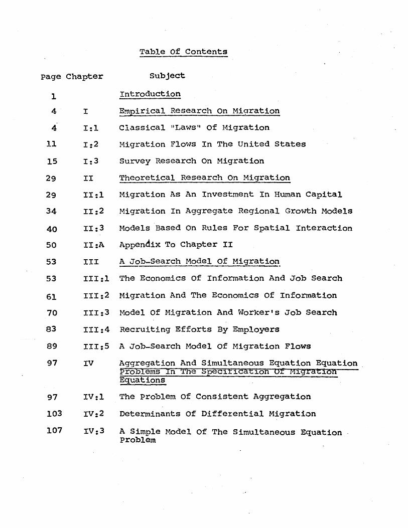
Table Of Contents
page Chapter Subject
1 Introduction
4 I Empirical Research On Migration
4 1:1 Classical "Laws" Of Migration
11 1:2 Migration Flows In The United States
15 1:3 Survey Research On Migration
29 II Theoretical Research On Migration
29 11:1 Migration As An Investment In Human Capital
34 11:2 Migration In Aggregate Regional Growth Models
40 11:3 Models Based On Rules For Spatial Interaction
50 II:A Appendix To Chapter II
53 III A Job-Search Model Of Migration
53 III:1 The Economics Of Information And Job Search
61 111:2 Migration And The Economics Of Information
70 111:3 Model Of Migration And Worker's Job Search
83 111:4 Recruiting Efforts By Employers
89 111:5 A Job-Search Model Of Migration Flows
97 IV Aggregation And Simultaneous Equation EquationProblems In The Specirication or MigrationEquations
97 IV:1 The Problem of Consistent Aggregation
103 IV:2 Determinants Of Differential Migration
107 IV:3 A Simple Model Of The Simultaneous EquationProblem
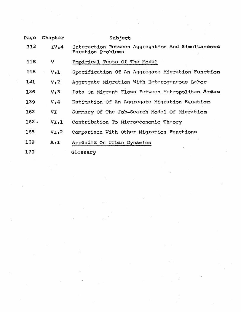
Page Chapter
113
118
118
131
136
139
162
162-
165
169
170 Glossary
IV:4 Interaction Between Aggregation And SimultanecxtsEquation Problems
V Empirical Tests Of The Model
V:l Specification Of An Aggregace Migration Functioin
V:2 Aggregate Migration With Heterogeneous Labor
V:3 Data On Migrant Flows Between Metropolitan Aetas
V:4 Estimation of An Aggregate Migration Equation
VI Summary of The Job-Search Model of Migration
VI:l Contribution To Microeconomic Theory
VI:2 Comparison With other Migration Functions
A:I Appendix On Urban Dynamics
Subject
1
INTRODUCTION
Streams of human migration have had overwhelming
sociological, cultural, and economic consequences, Nowhere
is this more true than in the United States which is today
peopled by the offspring of immigrants and continues to
eXperience high rates of internal migration among its
culturally and economically diverse sub-regions. For example,
the movements of Negroes out of the rural South and Puerto
Ricans from the Commonwealth of Puerto Rico to the middle
atlantic states imply profound and probably unique social and
cultural changes on the part of the migrants.
There are also important effects arising from the move.
ment of a relatively homogeneous population within a system of
urban areas. Such migration involves little cultural change
but its potential economic impact in countries like the United
Stateswhere one in eight families changes its county of
residence each year, is great. This thesis attempts to model
the movement of homogeneous populations as opposed to unique
population movements discussed earlier. Migration is treated
as a purely economic process of labor market adjustment. The
analysis developed here should not be applied directly to
unique flows of heterogeneous population groups where important
cultural change accompanies migration. However, just as the
2
perfectly competitive ideal provides a framework for inter-
preting oligopoly, the abstract and idealized approach adopted
here for movement of homogeneous populations should provide a
basis for understanding unique population movements, Indeed
there is some evidence that historical migrations between
diverse regions or from rural to urban areas have exhibited
some empirical regularities which may be due to common
underlying economic factors,
Migration between metropolitan areas is an important
determinant of regional and urban growth patterns, Under-
standing and predicting population flows is vital to rational
planning for urban development. In some metropolitan areas,
such as Washington and Los Angeles, net in-migration has been
more important than natural increase in accounting for the
growth of population, In such areas planning programs which
relied on population projections based on natural increase
alone would result in inadequate provision of public facilities,
Ccnversely, the majority of counties in the United States
experienced a fall in population between 1960 and 1970 due to
out-migration in excess of natural increase. Here excessive
investment in public facilities would result from planning
based on projected natural increase,
Recently migration has become important in another
context, Persistent differences in wages and unemployment
1This issue is discussed in Chapter I:1,
3
rates among areas have led to speculation that present levels
and/or patterns of migration are not efficiently moving labor
services from areas of surplus to those with current shortages.
In this context migration is seen as an investment in human
capital which has a rate of return that is sufficiently high
to indicate that market processes are not allocating sufficient
funds to migration. Thus increasing investment in migration
is viewed as a short-run strategy to shift the Phillips curve
and as a long-run answer to problems of lagging regions.
Resolution of the debate over optimal migration must wait upon
the formulation of positive models of the migration process
which relate to the body of microeconomic theory. The models
developed here represent an attempt at such a formulation.
Chapters I and II of this thesis review empirical data
on migration flows and existing analytical models of migration
processes. In Chapter III an analytic theory of migration is
developed based on a job-search model of the labor market.
Problems of simultaneous equation bias and inconsistent
aggregation inherint in any attempt to estimate migration
equations are reviewed in Chapter IV. Chapter V contains
estimates of aggregate migration equations for the United
States and the United Kingdom. A summary of results and
conclusions follows in Chapter VI.
I -- "I I" F V, I I , 0.1 W- row MW , R 7 1 1 -, I
4
Chapter I
EMPIRICAL RESEARCH ON MIGRATION
The limited nature of migration data sources has long
inhibited empirical work on migration processes. The three
sections of this chapter relate roughly to the three tradi-
tional sources of data on migrants, net migration flows based
on census data on changes in population 7 gross migration flows
obtained from census questions concerning place of residence
one or five years earlier? and surveys of migrants designed
to determine reasons for mobility. Various descriptive
statistics computed from these data suggest a variety of
persistent empirical regularities that appear to characterize
migrants and migration processes. Any microeconomic theory
of migration should be consistent with the more well-estab .a.
lished empirical generalizations.
I:1) Classical "Laws" of Migration
The primary data sources available to demographers since
the sixteenth and seventeenth centuries were bills of mortality
and certificates of baptism recorded in larger cities, From
these data and population totals practitioners of "Political
Arithmetic," as demography was then named, were able to
construct estimates of net migration, They found very
strong patterns of population flows from rural areas and
1 0 1 U.-V91r1w
5
small towns to great cties. Until the nineteenth century
most large european cities had an excess of deaths over
births accompanied by substantial population increases.
Improved sanitation and medical practice lowered death rates
in cities. By the mid-nineteenth century, natural increase
was a more important factor in London's population growth
than it had been in the seventeenth century, although rural
immigration flows were still substantial. Net inmigration
was about 6000 per year in 1650 and 11,000 annually in 1870
but the population of London had increased by a factor of
ten during this period.2
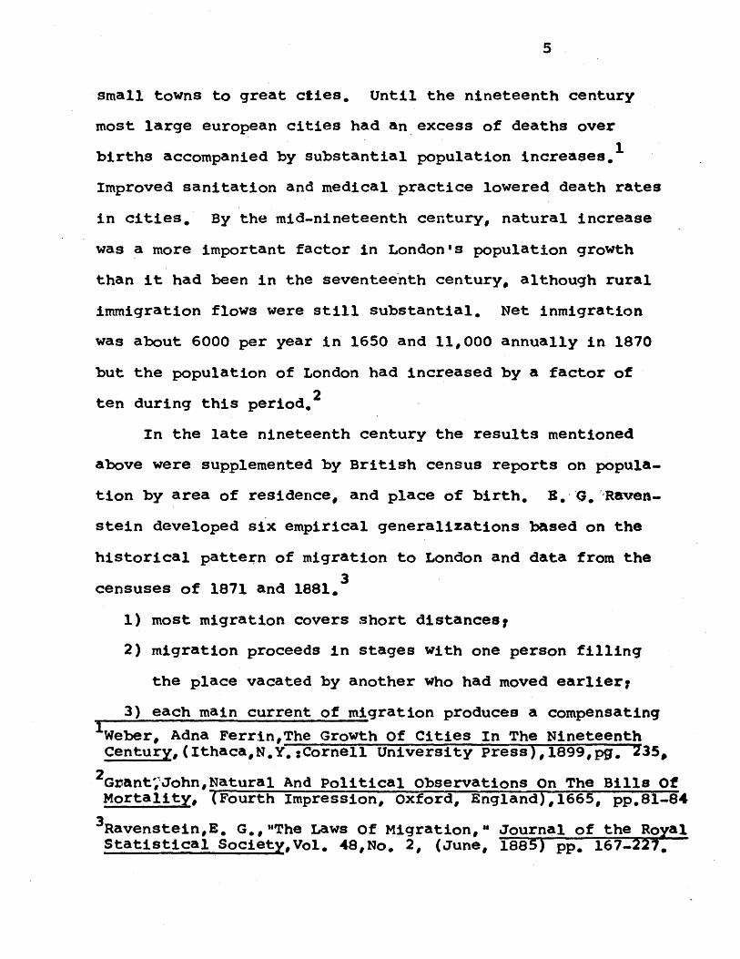
In the late nineteenth century the results mentioned
above were supplemented by British census reports on popula-
tion by area of residence, and place of birth. B. -'G.Raven-
stein developed six empirical generalizations based on the
historical pattern of migration to London and data from the
censuses of 1871 and 1881.3
1) most migration covers short distancest
2) migration proceeds in stages with one person filling
the place vacated by another who had moved earliery
3) each main current of migration produces a compensating
Weber, Adna Ferrin,The Growth Of Cities In The NineteenthCentury, (Ithaca,N.Y.:Cornell University Press),1899,pg. 235,
2 Grant'JohnNatural And Political observations On The Bills OfMortality, (Fourth Impression, Oxford, England),1665, pp.81-84
3Ravenstein,E. G.,"The Laws Of Migration," Journal of the RoyalStatistical Society,Vol. 48,No. 2, (June, 1885) pp. 167-227.
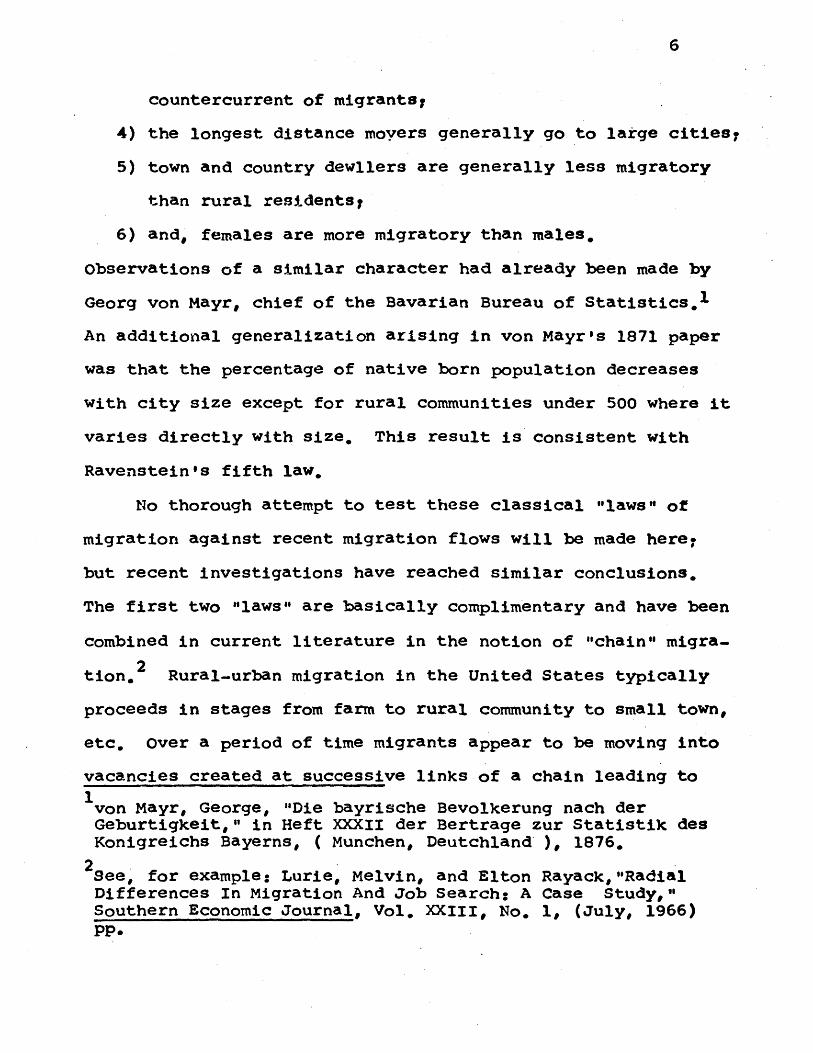
6
countercurrent of migrants7
4) the longest distance moyers generally go to large cities7
5) town and country dewllers are generally less migratory
than rural residents7
6) and, females are more migratory than males.
observations of a similar character had already been made by
Georg von Mayr, chief of the Bavarian Bureau of Statistics.1
An additional generalization arising in von Mayr's 1871 paper
was that the percentage of native born population decreases
with city size except for rural communities under 500 where it
varies directly with size. This result is consistent with
Ravenstein's fifth law,
No thorough attempt to test these classical "laws" of
migration against recent migration flows will be made here7
but recent investigations have reached similar conclusions.
The first two "laws" are basically complimentary and have been
combined in current literature in the notion of "chain" migra-.
tion.2 Rural-urban migration in the United States typically
proceeds in stages from farm to rural community to small town,
etc, over a period of time migrants appear to be moving into
vacancies created at successive links of a chain leading to
von Mayr, George, "Die bayrische Bevolkerung nach derGeburtigkeit," in Heft XXXII der Bertrage zur Statistik desKonigreichs Bayerns, ( Munchen, Deutchland ), 1876.
2See, for example: Lurie, Melvin, and Elton Rayack,"RadialDifferences In Migration And Job Search: A Case Study,"Southern Economic Journal, Vol. XXIII, No. 1, (July, 1966)pp.
. 11 I I", " 41F. , I " if - 09 - - -- - ___1 - - -
7
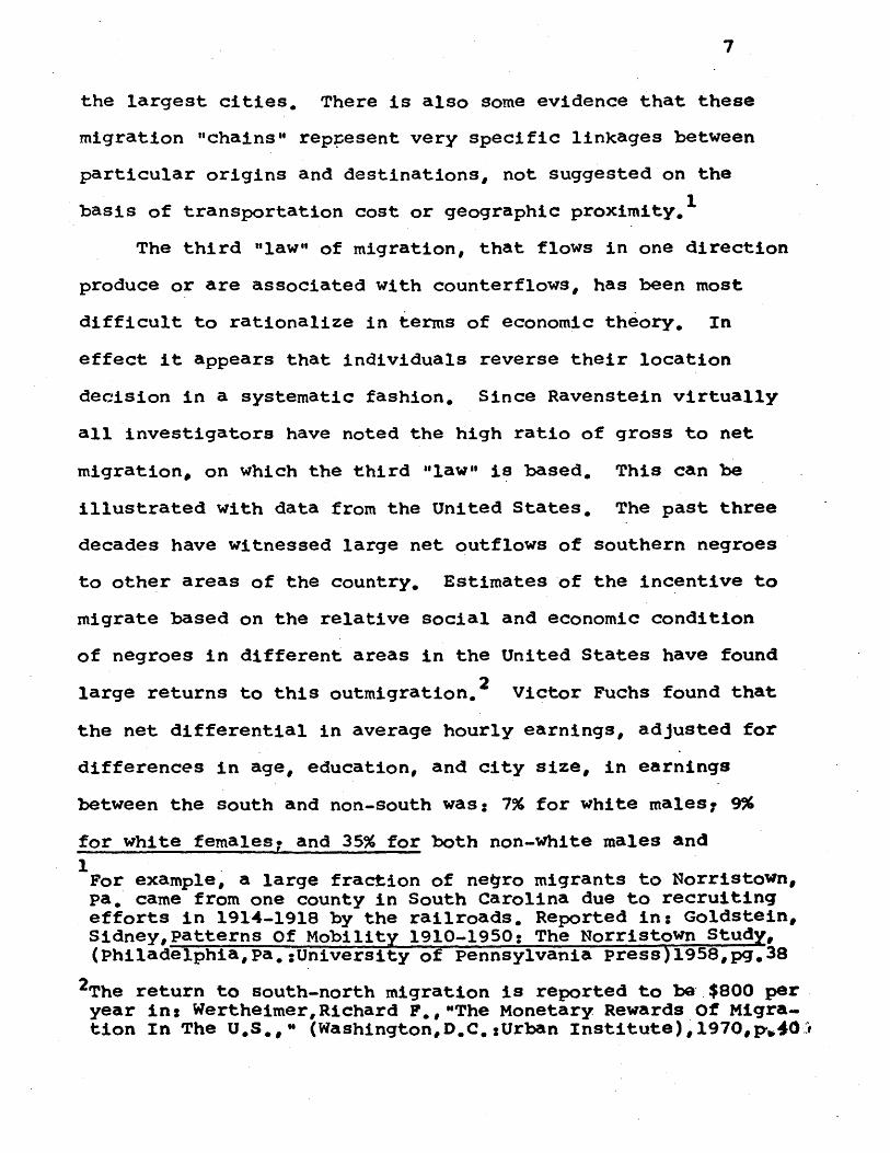
the largest cities. There is also some evidence that these
migration "chains" reppesent very specific linkages between
particular origins and destinations, not suggested on the
basis of transportation cost or geographic proximity.
The third "law" of migration, that flows in one direction
produce or are associated with counterflows, has been most
difficult to rationalize in terms of economic theory. In
effect it appears that individuals reverse their location
decision in a systematic fashion. Since Ravenstein virtually
all investigators have noted the high ratio of gross to net
migration, on which the third "law" is based. This can be
illustrated with data from the United States. The past three
decades have witnessed large net outflows of southern negroes
to other areas of the country. Estimates of the incentive to
migrate based on the relative social and economic condition
of negroes in different areas in the United States have found
2large returns to this outmigration. Victor Fuchs found that
the net differential in average hourly earnings, adjusted for
differences in age, education, and city size, in earnings
between the south and non-south was: 7% for white males? 9%
for white femaleso and 35% for both non-white males and
For example, a large fraction of negro migrants to Norristown,Pa. came from one county in South Carolina due to recruitingefforts in 1914-1918 by the railroads. Reported in: Goldstein,Sidney,Patterns Of Mobility 1910-1950: The Norristown Study(Philadelphia,Pa.:University of Pennsylvania press)1958,pg.38
2The return to south-north migration is reported to be.$800 peryear in: Wertheimer,Richard F.,"The Monetary Rewards of Migra-tion In The U.S.," (Washington,D.C.:Urban Institute),1970,p.40i
q- q, mw _1W,10P "''I Is ". @ -I- I I ____ ___
8
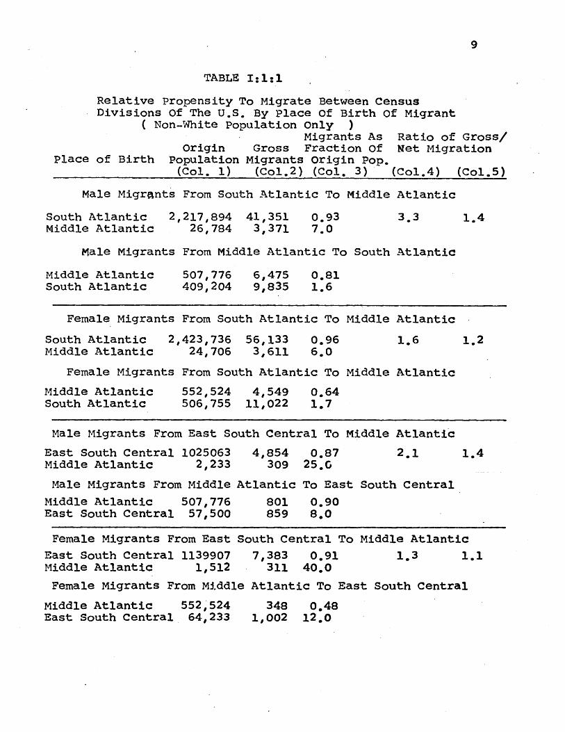
females.I As Table 1:1:1 below indicates, the gross flows
which characterize non-white migration between southern and
northern census divisions are seldom less than twice and
usually more than thrice as large as net flows. Thus even
in the presence of very large incentives to migration in
one directionsbuth to north, there are large flows in the
opposite direction.
Furthur examination shows that the flow of non-whites to
the south consists largely of individuals born in the south
who previously migrated to the north. Column 3 of Table I:1:1
indicates that return migrants were in all cases far more
important in itigration flows than their numbers would indicate,
being over-represented in north to south migration flows by
a factor of 6 or 7 to as much as a factor of 40. Considering
migration flows net of migrants returning to their division
of birth, in column 5 of Table I:1:1, gives much more
decisive ratios of gross to net migration. Thus the high
ratio of gross to net migration for non-white population
movements is due largely to return migration -by individuals
born in the south who moved north earlier. This gives some
additional insight into Ravenstein's third "law" but it is
far from providing an understanding of the causes of the
countercurrents that accompany initial migration flows,
1 Fuchs, Victor R.,"Differentials In Hourly Earnings ByRegion And City Size, 1959," occasional Paper #101, (NewYork:National Bureau of Economic Research), 1967.
9
TABLE 1:1:1
Relative Propensity To Migrate Between CensusDivisions Of The U.S. By Place of Birth Of Migrant
( Non-White Population Only )Migrants As Ratio of Gross/
Origin Gross Fraction Of Net Migration
(Col.4) (Col.5)Place of Birth Population Migrants Origin Pop.
(Col. 1) (Col.2) (Col. 3)
Male Migrants From South Atlantic To Middle Atlantic
South Atlantic 2,217,894 41,351 0.93 3.3 1.4Middle Atlantic 26,784 3,371 7.0
Male Migrants From Middle Atlantic To South Atlantic
Middle Atlantic 507,776 6,475 0.81South Atlantic 409,204 9,835 1.6
Female Migrants From South Atlantic To Middle Atlantic
South AtlanticMiddle Atlantic
2,423,736 56,13324,706 3,611
Female Migrants From South Atlantic To Middle Atlantic
Middle AtlanticSouth Atlantic
552,524 4,549506,755 11,022
Male Migrants From East South Central To Middle Atlantic
East South Central 1025063Middle Atlantic 2,233
4,854 0.87309 25.0
Male Migrants From Middle Atlantic To East South Central
Middle Atlantic 507,776 801 0.90East South Central 57,500 859 8,0
Female Migrants From East South Central To Middle Atlantic
East South Central 1139907Middle Atlantic 1,512
7,383 0.91311 40.0
1.3
Female Migrants From Middle Atlantic To East South Central
Middle Atlantic 552,524East South Central 64,233
348 0.481,002 12.0
0.966.0
1.6 1.2
0.641.7
2.1 1.4
1.1

10
TABLE 1:1:1(continued)
Descriptions Of Census Divisions
Middle Atlantic Census Division - Maryland, District ofColumbia, Pennsylvania, Deleware, New Jersey, andNew York.
South Atlantic Census Division - Virginia, North Carolina,South Carolina, Georgia, and Florida.
East South Central Census Division - Alabama, Mississippi,Kentucky, and Tennessee
Notes on the Calculations in the Table
Column 3 migrants as a fraction of population at the
origin, is equal to the ratio of gross migrants, column 2,
and origin population* column 1. The ratio of gross to net
migration in column 4 is equal to the difference in gross
migrants in each direction divided by the sum of gross
migrants in column 2. The ratio of gross to net migration
in column 5 is calculated in similar manner with return
migrants eliminated from the calculation,
1 U.S. Bureau of the Census, U.S. Census of Population: 1960Subject Reports 4 Mobility for States and Economic Areas,Final Report PC(2)-2B, (Washington, D.C.: U.S. GovernmentPrinting office); 1963.
11
The last three classic "laws" of migration are fairly
innocuous but they are essentially consistent with data on
recent migration flows in the United States. The robustness
of these calssic observations on migration, now about to
enter their second century, is quite remarkable. There has
been a consistent tendency to ignore much of this early work
on migration in spite of its continued validity. Perhaps
this is due to the failure of recent migration models to
account for behavior characteristic of classic migration
studies. The job-search model of migration presented here
accounts for most of the classic results that still apply
today.
1:2) Migration Flows In The United States
In her 1938 summary of research on migration, Dorothy
Swain Thomas disparaged the state of inquiry in the United
States as "trivial and inept."1 Her criticism was not only
based on the lack of specific data on population flows. The
problem with past research centered on the lack of imagina-
tive analytical approaches to the p.vailable data.
Kuznets and Miller analyzed changes in the composition
of population in different states and regions that occured
Thomas, Dorothy S., Research Memorandum On MigrationDifferentials, (New York:Social Science Research Council),1938, pg. 160.
12
between 1870 and 1950. They found a continuous reduction in
the divergence among the proportions of state populations
comprising different age, sex, and race groups. In her
analysis of state work forces, Miller noted a convergence of
indicators such as labor force participation rates and the
proportion of employment in each of eight industrial categor~.
ies. The sum of the divergence of deviations of individual
states from the national average for most labor force indic-
ators decreased steadily from 1890 to 1950.2 This indicates
an equilibrating effect of net migration which is consistent with
neoclassical models of economic growth in the absence of
barriers to factor mobility.
Analysis of indirect indicators of the effect of geogra-
phic labor mobility has also revealed fundamental long-run
leveling processes. Most significant has been the conver-
gence of income per capita and wages per manhour. Easterlin's
index of the average deviation of income per capita among
states fell almost fifty percent between 1927-32 and 1944-48,
and remained constant from then until his last computation for
1953-55.3 Subsequent work on changes in relative wages among
regions has shown similar convergence followed by stability,1 Kuznets, Simon, Ann Rather Miller, and Richard A. Easterlin,Population Redistribution And Economic Growth,(Philadelphia:American Philosophical Society), 1960.
2 Kuznets, Simon, et, al., Ibid, pp. 7-101.
3Easterlin, Richard A.,"Interregional Differences In Per CapitaIncome, 1840-1950," Vol. 24, National Bureau of Economic Res-darch, Conference on Research In Income And Wealth,(1960).
13
particularly of the north-south money wage ratio, in the post
World War II period. Of course both supply and demand pheno-
mena produce movements in relative wages in different regions.
The recent stability of relative wages and per capita income
may be due to a long-run equilibrium of some sort or result
from compensating labor supply and demand effects that are
temporarily in balance. However there is little doubt that
migration has contributed to the stability of relative wages
among regions in recent years. The lowest income states have
experienced net outflows of migrants and the highest income
2states have been gaining population through migration. Thus,
in spite of the rise of countercurrents or reverse migration,
the overall effect of migration flows on labor markets has
been to shift population in a manner consistent with the
elimination of income differentials among regions.
The inclusion of a question on migration in the 1940
U.S. Census of Population made possible the analysis of
characteristics of migrants. Differential migration studies
compared the proportion of a population subgroup that migrated
with the average ratio of migrants to population.
Crosstabulations of the population, such as those found
1Kuznets, Simon, et, al., o_. cit., pg. 171.
A review of the relative wage literature appears in: Galaway,L.,"The North-South Wage Differential,," Review of EconomicsAnd Statistics, XLV, (1963), pp. 264-272*
14
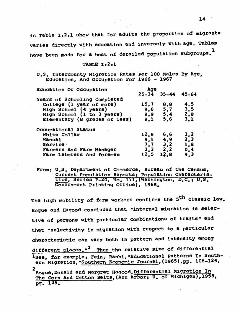
in Table 1:2:1 show that for adults the proportion of migrants
varies directly with education and inversely with ace. Tables
have been made for a host of detailed population subgroups.
TABLE 1:2:1
U.S. Intercounty Migration Rates Per 100 Males By Age,Education, And Occupation For 1966 - 1967
Education Ot Occupation Age25-34 35-44 45-64
Years of Schooling CompletedCollege (1 year or more) 15.7 8.8 4.5High School (4 years) 9.6 5.7 3.5High School (1 to 3 years) 9.9 5.4 2.8Elementary (8 grades or less) 9.1 5.6 3.1
Occupational StatusWhite Collar 12.8 6.6 3.2Manual 9.1 4.9 2*3Service 7.7 3.2 1.8Farmers And Farm Manager 3.3 2.2 0.4Farm Laborers And Foremen 12.5 1?.8 9.3
From: U.S. Department of Commerce, Bureau of the Census,Current Population Reports: Population Characteris-tics, Series P-20, No. 171,(Washington, D.C.: U.S.Government Printing Office), 1968.
The high mobility of farm workers confirms the 5th classic law.
Bogue and Hagood concluded that "internal migration is selec-
tive of persons with particular combinations of traits" and
that "selectivity in migration with respect to a particular
characteristic can vary both in pattern and intensity among2a
different places."2 Thus the relative size of differential
lSee, for example: Fein, Rashi,"Educational patterns In South-
ern Migration, "Southern Economic Journal, (1965),pp. 106-124.
2BogueDonald and Margret HagoodDifferential Migration In
The Corn And Cotton Belts, (Ann Arbor: U. of Michigan),1953,pg. 125.
15
migration flows among areas depend on the characteristics of
the areas as well as those of the population subgroups
involved. For example, in the case of migrants to Miami Beach,
Florida, there might be a positive association between age
and relative migrant flows. This is inconsistent with the
relative migration rates observed for the entire nation and
reflects particular characteristics of the area.
1:3) Survey Research On Migration
The most detailed information on migrants comes from
large surveys of the population. Thus far the masses of
survey data and related results have been largely ignored in
more theoretical research. Two sorts of information have
resulted from surveys. First it has been possible to compare
the characteristics of migrants with those of the population
in general. Secondly unique insights into the rationale for
migration and the migration decision itself are available in
terms of the perceptions of the migrants themselves.
A commonly stated objective of surveys of migrants has
been the determination of the importance of "economic consid-.
erations" in general and employment opportunities specifically
in motivating migration between areas. Unfortunately many
surveys have interpreted "economic" reasons for moving very
narrowly. Thus an "economic rationale" for moving typically
16
includes only responses that indicate a move was designed to:
take a job already offered* look for work7 or to complete a
job transfer. Housing problems, health problems, general
cost of living, and "community considerations" are inevitably
classified as non-economic reasons for moving. No attempt is
made to determine if housing or health facilities were
completely unavailable at the origin of the move or whether
they were merely more expensive than at the destination. This
approach indicates complete money illusion on the part of the
survey researchers. The possibility that this also reflects
money illusion on the part of migrants will be discussed
later.
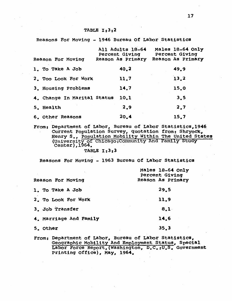
In spite of the narrow definitions used, a majority of
all respondents in all surveys reported that they moved
primarily for "economic reasons.' 1" Job transfers or taking a
new job dominated the responses of those who reported that
they moved for economic reasons. In general only about
twenty percent of those who reported that they moved for
economic reasons moved in order to look for a job that had
not been prearranged. The full results of four surveys that
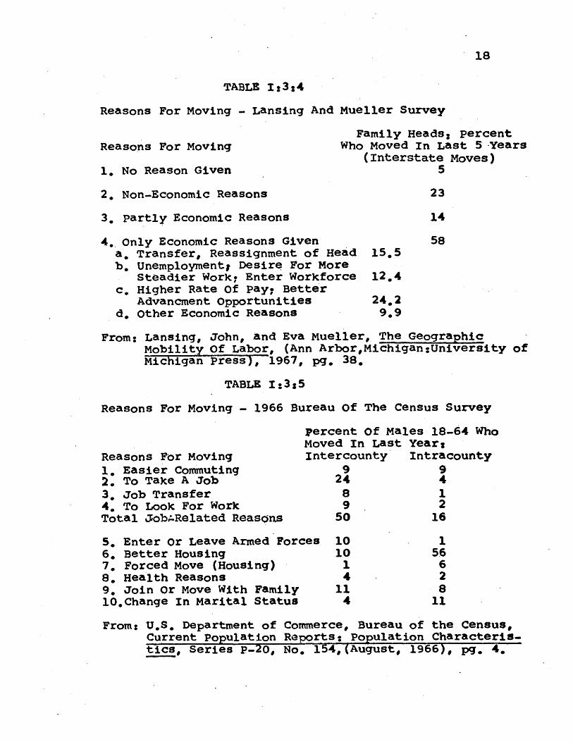
attempted to deduce the reasons for moving are given in
Tables 1:3:2 through 1:3:5 below. Results of similar questions
asked intra-county migrants are also presented to indicate
1This generalization is based on the four studies mentionedin the tables below.
17
TABLE 1:3:2
Reasons For Moving - 1946 Bureau Of Labor Statistics
All Adults 18-64 Males 18-64 OnlyPercent Giving Percent Giving
Reason For Moving Reason As Primary Reason As Primary
1. To Take A Job 40.2 49.9
2. Too Look For Work 11.7 13.2
3. Housing Problems 14.7 15*0
4. Change In Marital Status 10.1 3*5
5. Health 2.9 2.7
6. Other Reasons 20.4 15.7
From: Department of Labor, Bureau of Labor Statistics, 1946Current Population Survey, quotation from: Shryock,Henry S., Population Mobility Within The United States(Universit of Chicago:Community And Family StudyCenter), 64.
TABLE 1:3:3
Reasons For Moving - 1963 Bureau Of Labor Statistics
Males 18-64 onlyPercent Giving
Reason For Moving Reason As Primary
1. To Take A Job 29.95
2. To Look For Work 11.9
3. Job Transfer 8.1
4. Marriage And Family 14.6
5. Other 35.3
From: Department of Labor, Bureau of Labor Statistics,Geographic Mobility And Employment Status, SpecialLabor Force Report, (Washington, D.C.:U.S. GovernmentPrinting Office), May, 1964.
18
TABLE 1:3:4
Reasons For Moving - Lansing And Mueller Survey
Reasons For Moving
1. No Reason Given
2, Non-Economic Reasons
3. Partly Economic Reasons
Family Heads: PercentWho Moved In Last 5 -Years
(Interstate Moves)5
23
14
4. Only Economic Reasons Givena. Transfer, Reassignment of Head 15.5b, Unemploymentj Desire For More
Steadier Work? Enter Workforce 12,4c. Higher Rate of Pay. Better
Advancment Opportunities 24.2d, Other Economic Reasons 9.9
58
From: Lansing, John, and Eva Mueller, The GeographicMobility Of Labor, (Ann ArborMichigan:University ofMichigan Press), 1967, pg. 38.
TABLE I:3:5
Reasons For Moving - 1966 Bureau Of The Census Survey
Reasons For Moving1. Easier Commuting2. To Take A Job3. Job Transfer4. To Look For WorkTotal Job.Related Reasons
percent Of Males 18-64 WhoMoved In Last Year:Intercounty Intracounty
9 924 489
50
5. Enter Or Leave Armed Forces 106. Better Housing 107. Forced Move (Housing) 18. Health Reasons 49. Join Or Move With Family 11l0.Change In Marital Status 4
12
16
156628
11
From: U.S. Department of Commerce, Bureau of the Census,Current Population Reports: Population Characteris.-tics, Series P-20, No, 154, (August, 1966), pg. 4.
19
the diminished importance of job-related reasons for moving
as the distance covered decreases.
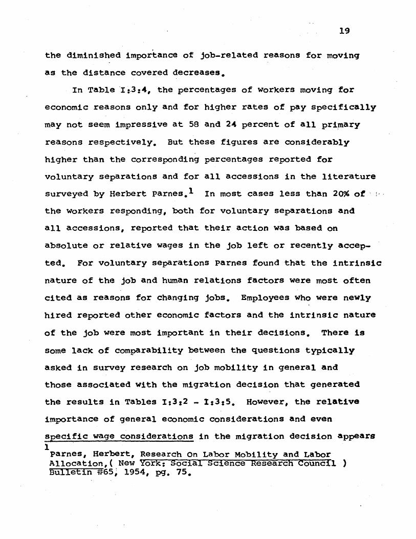
In Table I:.3:4, the percentages of workers moving for
economic reasons only and for higher rates of pay specifically
may not seem impressive at 58 and 24 percent of all primary
reasons respectively. But these figures are considerably
higher than the corresponding percentages reported for
voluntary separations and for all accessions in the literature
surveyed by Herbert Parnes. 1 In most cases less than 20% of
the workers responding, both for voluntary separations and
all accessions, reported that their action was based on
absolute or relative wages in the job left or recently accep-
ted. For voluntary separations Parnes found that the intrinsic
nature of the job and human relations factors were most often
cited as reasons for changing jobs. Employees who were newly
hired reported other economic factors and the intrinsic nature
of the job were most important in their decisions. There is
some lack of comparability between the questions typically
asked in survey research on job mobility in general and
those associated with the migration decision that generated
the results in Tables 1:3:2 - 1:3:5. However, the relative
importance of general economic considerations and even
specific wage considerations in the migration decision appears
parnes, Herbert, Research On Labor Mobility and LaborAllocation,( New York: Social Science Research Council )Bulletin #65, 1954, pg, 75.
20
to be comparable to the relative importance of these consid.
erations in other labor mobility decisions. The results of
this survey information on the migration decision indicate
a large fraction of all migration is based on an economic
and job-related rationale, This "large fraction" compares
favorably with that found for other forms of labor mobility
traditionally analyzed with rather conventional economic
models. Thus there appears to be great promise for economic
models of the migration decision.
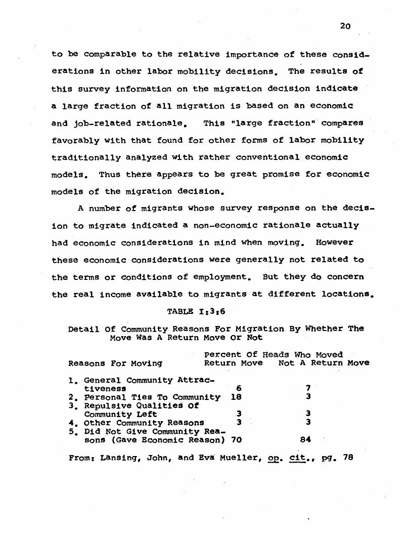
A number of migrants whose survey response on the decis-
ion to migrate indicated a non-economic rationale actually
had economic considerations in mind when moving. However
these economic considerations were generally not related to
the terms or conditions of employment. But they do concern
the real income available to migrants at different locations,
TABLE 1:3:6
Detail Of Community Reasons For Migration By Whether TheMove Was A Return Move or Not
Percent Of Heads Who MovedReasons For Moving Return Move Not A Return Move
1. General Community Attrac-tiveness 6 7
2. Personal Ties To Community 18 33. Repulsive Qualities of
Community Left 3 34. Other Community Reasons 3 35. Did Not Give Community Rea-
sons (Gave Economic Reason) 70 84
From: Lansing, John, and Eva Mueller, op. cit., pg. 78
21
Table 1:3:6 presents a detailed examination of the respondents
to the Lansing and Mueller survey who reported that they
moved for non-economic reasons. By far the most important
non-economic category of reasons for migration concerned
community reasons. "General community attractiveness" and
"repulsive qualities of community left" account for about
half of the community reasons for migration. This reflects
the importance among primary responses of essentially
consumption-related rationale for migration, based on: cost
of living7 climate* physical design; public goods availabilityl
and related factors. Such a consumption-related rationale for
migration is as much a part of real income considerations
as unemployment or money wage levels at different locations.
Indeed, it would be surprising if secondary responses of
those who moved primarily for job-related reasonsdid not
consider consumption characteristics of the destination in
weighing different locations. Unfortunately tabulations of
secondary reasons for migrating are not generally available.
Surveys of migrants are capable of providing even more
detailed insight into the nature of the migrants' decision
making process. Specifically characteristics of the extent
and pattern of deliberation involved in the migration decision
as well as the information used appears in the work of John
Lansing and Eva Mueller, Much of the remainder of this1Lan&ifg, John, and Eva Mueller, gg cit., Chapter IV.
22
relies on their work.
In general the length of time over which the migration
decision is considered is short. Only 34% of the households
that migrated in the Lansing and Mueller sample reported a
period of serious deliberation in excess of six months,
Indeed, 34% of the households considered the move seriously
for one month or less. A follow-up survey one year later on
those who reported that they might move in the next year
confirmed the indications of short deliberation periods. Only
40% of those who said that they definitely planned to move
had moved one year later and 3% of those who had no plans to
move actually moved. Since the latter group who had no moving
plans was far larger in absolute numbers than those who
anticipated moving, the group of actual movers one. year later
contained a majority of individuals who had no plans' to move
in the first survey. This indicates that the period of
deliberation given to both the decision to migrate at all and
to the exact destination of the move is short. Time constraints
placed on job offers and transfers may account for some of this
suddenness in the migration decision, but the haste with which
families decide to move is still surprising.
Another important attribute of the migration decision is
the sources of information which migrants use in deciding to
1Lansing, John, and Eva Mueller, o2. cit., pp. 209--210.
23
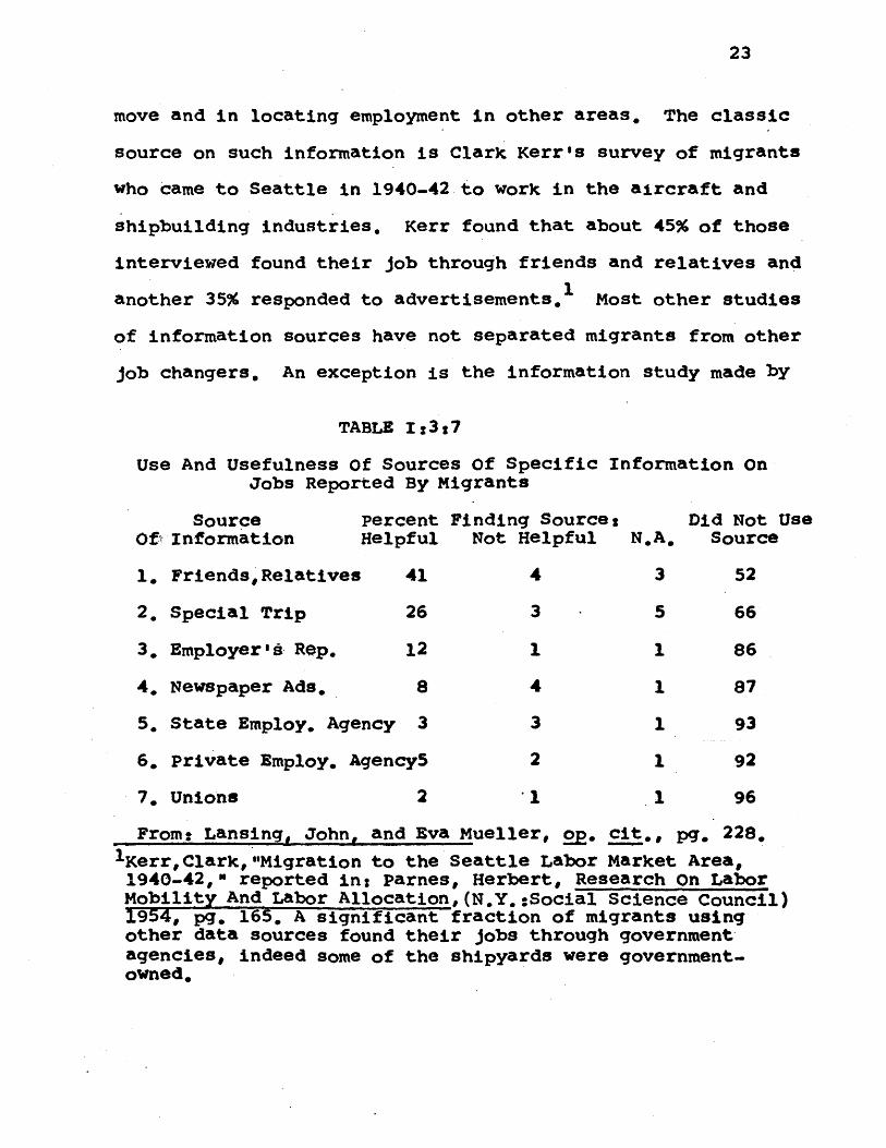
move and in locating employment in other areas. The classic
source on such information is Clark Kerr's survey of migrants
who came to Seattle in 1940-42 to work in the aircraft and
shipbuilding industries. Kerr found that about 45% of those
interviewed found their job through friends and relatives and
another 35% responded to advertisements. Most other studies
of information sources have not separated migrants from other
job changers. An exception is the information study made by
TABLE 1:3:7
Use And Usefulness Of Sources of Specific Information onJobs Reported By Migrants
Source Percent Finding Source: Did Not UseOft Information Helpful Not Helpful N*A. Source
1. FriendsRelatives 41 4 3 52
2. Special Trip 26 3 5 66
3. Employers *Rep. 12 1 1 86
4. Newspaper Ads. 8 4 1 87
5. State Employ. Agency 3 3 1 93
6. Private Employ. Agency5 2 1 92
7. Unions 2 ' 1 96
From: Lansing, John, and Eva Mueller, o. c., pg. 228.
1KerrClark, "Migration to the Seattle Labor Market Area,1940-42," reported in: parnes, Herbert, Research On LaborMobility And Labor Allocation, (N.Y. :Social Science Council)1954, pg. 165. A significant fraction of migrants usingother data sources found their jobs through governmentagencies, indeed some of the shipyards were government-owned.
24
Lansing and Mueller and reproduced in Table 1:3:7. The
importance of isolating information sources used by migrants
can be seen from the Lansing and Mueller analysis. Because
migrants are relatively heavily concentrated in white collar
occupations and must secure information on jobs at a distance,
they tend to rely on a different combination of information
sources than job changers in general. Friends and relatives
are the most important sources of information and are most
imstrumental in finding jobs for all classes of migrants and
job changers. But migrants tend to rely on special trips
and employer's representatives to provide specific information
on job opportunities. Newspaper advertisements, state employ-
ment agencies, private employment agencies, and unions are
among the sourcesused infrequentlyor neglected completely.
The combination of short deliberation periods and limited
and imprecise sources of information on job opportunities
suggests that, for most workers, the migration decision is a
creature of limited rationality at best. Certainly the
results discussed thus far indicate that the search for
employment is limited in extent. Most workers probably have
close relatives and friends at few other locations while
special trips and employer representatives are very specific
and limited sources of information about economic conditions
in other areas.
The relationship between migration and skill is in Ch. IV.
-1
25
Associated with the lack of extensive deliberation in the
migration decision is a failure to consider many alternative
locations. Indeed 64% of the Lansing and Mueller sample of
approximately 5,000 interstate movers said that they consider-
ed no alternative locations before moving. Even among
professional and technical woukers, who participate in broad
spatial labor markets, 56% considered only one destination..
For other white collar and blue collar workers the results
were 80% and 78% respectively. There was neither a strong
nor a uniform tendency for consideration of alternatives to
increase with longer deliberation periods. This does not
prove that individuals were unaware of employment opportunities
at other locations. But it is apparent that workers seldom
made an effort to investigate vacancies intensively in more
than one area other than their home. This confirms the
picture of a hasty migration decision painted earlier.
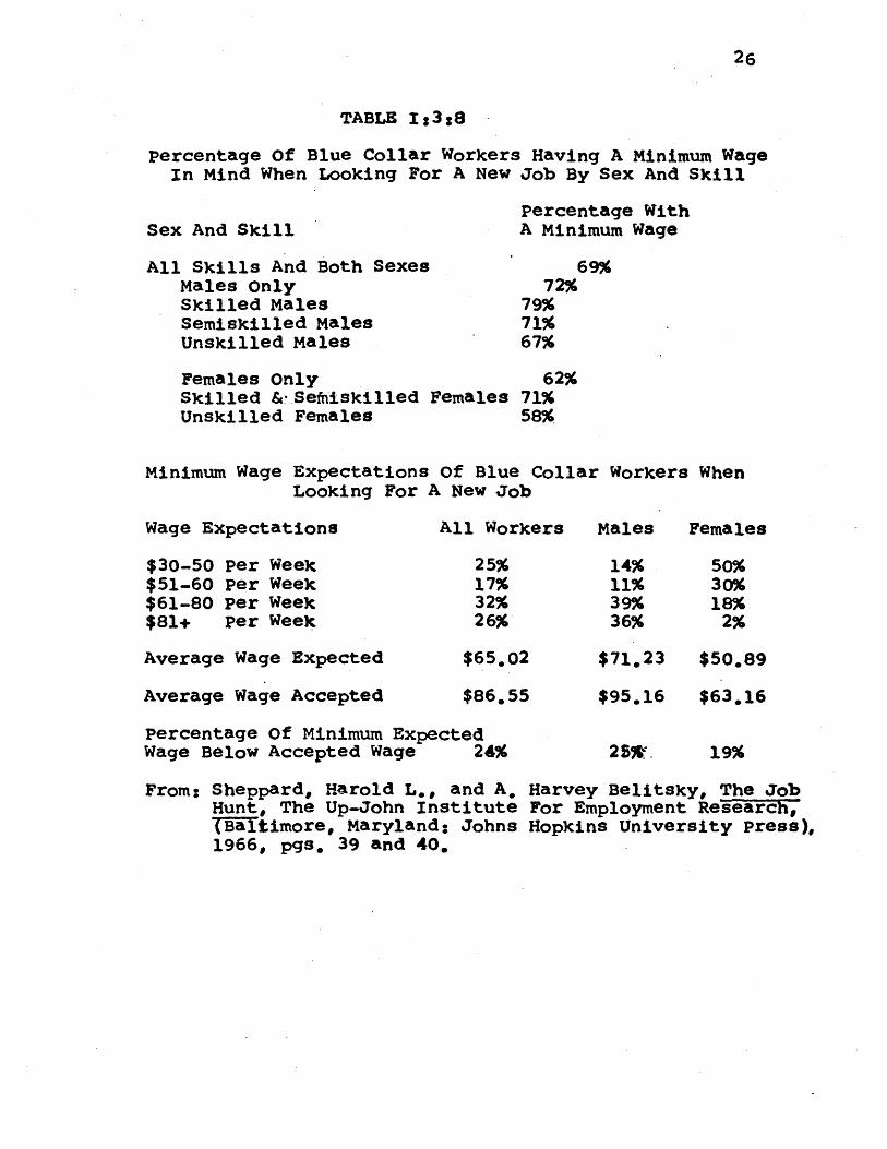
A final concept examined in the survey research liter-
ature on migration is the reservation wage. Surveys of
workers, particularly the unemployed, indicate that many
individuals attach a minimum wage to their labor services.
This minimum expected or reservation wage varies directly
with the skill level of the worker. Table 1:3:8 illustrates
this relationship.
1Lansing, John, and Eva Mueller, 2. cit., pg. 221.
26
TABLE 1:3:8
Percentage Of Blue Collar Workers Having A Minimum WageIn Mind When Looking For A New Job By Sex And Skill
Percentage WithSex And Skill A Minimum Wage
All Skills And Both Sexes 69%Males Only 72%Skilled Males 79%Semiskilled Males 71%Unskilled Males 67%
Females Only 62%Skilled &--Sefniskilled Females 71%Unskilled Females 58%
Minimum Wage Expectations Of Blue Collar Workers WhenLooking For A New Job
Wage Expectations All Workers Males Females
$30-50 Per Week 25% 14% 50%$51-60 Per Week 17% 11% 30%$61-80 Per Week 32% 39% 18%$81+ Per Week 26% 36% 2%
Average Wage Expected $65.02 $71.23 $50.89
Average Wage Accepted $86.55 $95.16 $63.16
Percentage Of Minimum ExpectedWage Below Accepted Wage 24% 2B5W. 19%
From: Sheppard, Harold L., and A. Harvey Belitsky, The JobHunt, The Up-John Institute For Employment Research,(Baltimore, Maryland: Johns Hopkins University Press),1966, pgs. 39 and 40.
27
It appears that about 70% of the workers in the sample on
which Table 1:3:8 is based had a form of reservation wage that
increased roughly with the skill and earnings expected for the
individual worker. Average wages in jobs actually accepted
by the workers surveyed were 20 to 25 percent higher than the
reservation or minimum expected wage. The study also deter-
mined that only 20 percent of the workers actually refused a
job offer. The divergence between accepted and reservation
wages and the small number of rejected job offers indicates
that workers were willing to take a job and continue search in
their spare time. It appears that average wages attached to
job vacancies in the area surveyed, ( Erie, Pennsylvania ),
were about 20 percent above the reservation wage. It would
appear that individuals who might accept a wage offer as low
as the reservation wage would plan on continueing their
search effort while employed. Indeed this intention to cont-
inue searching after accepting a position may explain the
relatively low level of reservation wages and the reluctance
of workers to turn down a job offer.
Unfortunately there has been no extensive investigation
of the importance of a reservation wage for samples consisting
exclusively of intercounty migrants. Unlike workers consider-
ing jobs in their home labor market' those who must migrate
--- -- -- - - . " -. 41 0 " M. I .--- - In I Wal"M ,
-28
to accept a new position are unlikely to plan additional
search in their local labor market. Thus for the migrant
the decision to accept a position at a distance reflects a
long-run commitment to employment in the destination labor
market. Similarly any reservation wage associated with
migration to a different area must be based on a.long-run
employment decision.
Results provided by the survey literature on migrants
will be a powerful source of empirical evidence for the
job-search model of migration developed here. The reserva-
tion wage will be among the most important of the concepts
derived from the survey literature.
29
CHAPTER II
THEORETICAL RESEARCH ON MIGRATION
There have been few attempts to develop models of the
determinants of migration processes that could be integrated
into the body of economic theory. An exception is the
attempt to analyze migration as an investment in human
capital. Another approach has involved the analysis of
migration as an equilibrating force in interregional growth
models. Finally a number of aggregate models of migrant
flows have been proposed based on "gravity" models and other
functional forms of spatial interaction that have proved use-
ful in geography and regional science.
II:1) Migration As An Investment In Human Capital
Most migration is undertaken not for the pleasure which
moving might bring, or for the stimulaten of new places, but
rather in order to obtain more satisfactory employment.
This implies that the individual undertakes costs of moving
in order to change the locaten of his labor services to an
area in which the productivity of these services could be
greater. Larry Sjaastad was the first author to propose that
migration be considered an investment in human capital, in the
same sense that changing the location of a piece of physical
The survey research literature reviewed in Chapter I indi-cates that as many as half of all moves are made primarilyfor employment-related reasons,
I -W -- EM No, R1 11 M -- W-W Rippe
30
capital represents an investment. When dealing with human
beings, however, there is some difficulty in distinguishing
consumption from investment. Nevertheless the human capital
model has had some success in explaining characteristics of
migration flows and patterns of differential migration.
Each individual at his initial location possesses a
stock of human capital including: education7 skills7 health?
job rights? location, etc. By selling the services of these
aspects of their labor services in the local labor market
workers can realize a stream of earnings over their working
lives. Earning streams are available at other locations to
individuals similarly endowed. The relative value of the
streams at different locations may be compared by finding the
appropriate discount rate, quantifying the costs involved in
migration, and computing the present value of the earnings
2over time. If the act of moving is an investment then
equilibrium among local labor markets is achieved when the
expected value of relative wages in different areas is such
1 Sjaastad, Larry A., "The Costs And Returns of Migration,"Journal Of Political Economy, Vol. LXX, (Oct. 1962), pp.8 0 -9 3.
2This computation is actually quite complex, depending on pro-per determination of the discount rate: expected value andvariance, or more generally the distribution of wages at alllocations? and the degree of risk preference of migrants. Iff( y , t ) is the probability density function of the differ-ence In wages between location i and j at time-t, and r isthe rate of discount, then the expected value of the presentvalue of migratio fom i to j is:
E(Vij) = 30 e-rt f( y ,t ) dy dt
where: T is the number of years until retirement
31
that the present value of changing the location of any
worker's human capital is not greater than moving costs, 1
This is essentially the same condition that cheracterizes an
equilibrium for any durable good in a system of markets with
positive transportation costs.
The descriptive statistics on migration in the United
States presented in Chapter I indicate that population flows
do not follow patterns characteristic of capital or durable
goods subject to positive transportation costs. First,
population movements follow particular paths connecting indi-
vidual origins and destinations in a fashion that ignores
2relative transportation costs. Secondly, even when the
apparent incentive to migrate is great, as measured by rela*.
tive wages or earnings, large reverse migration flows are
found. These reverse flows do not reflect an aggregation
problem, as has been suggested, with outmigrants having
different skills than immigrants.3 Indeed return migrants are
This doeg not imply equality of wages or earnings for similaroccupations even in a world of perfect competition. Scarceand immobile resources, such as favorable climate, are suf-ficient to insure wage differentials, However, the realincome or attractiveness at all locations will be equalized.
A number of authors have reported narrow migration paths thathave dominated the relationship between particular originsand destinations. This special association has been called"chain" migration. See, for example: Lurie, Melvin, andElton Rayack,!"Racial Diferences In Migration And Job Search,"Southern Economic Journal, Vol. XXIII, No. 1,(July,1966)
3This explanation of the high ratio of gross to net flows isoften offered in the human capital literature, See, forexample$ Sjaastad, Larry A., _p, cit., pg. 82.
- - - , WO 0 1 WPPP W R rm-M _ -_ --- - "M
32
relatively over-represented in the reverse migration flows.
Thus we are left with the curious picture of the migration
"investment" systematically reversing itself. It seems
unlikely that flows of capital equipment follow such a pattern.
Finally, differential migration rates for various age groups
cannot be explained, as is often claimed, on the basis of
differences in the present value of wage differentials due
to the longer working life of the young. Differences in the
present value of wage streams contributed by earnings
differentials after the first 25 years are quite small in
relation to the differential migration rates between the
25-29 and 30-35 year old age cohorts.1
As a positive theory of migration processes the human
capital approach leaves much to be desired, Data on actual
migration flows indicate substantially different patteras of
movement than those which would characterize movement of
durable goods in or among spatially differentiated markets.
The normative implications of the human capital approach
to migration have recieved most attention, Indeed the model
achieves much of its significance because it is consistent with
IThe relative migration rate of individuals 25-29 years of age,adjusted for differences in education, is 40% higher thanthat for individuals 30-34 years old. It seems unlikely thatmuch of this difference is due to the longer period of timewhich the younger group has until retirement. In ChapterIV:2 an alternate explanation for these migration differen-tials is discussed, The 30-34 year old cohort has 25 yearsuntil retirement and the present value of a $1000 earningsdifferential in annual earnings 25 years hence discountedat 6% is only $221.
M I . W lee, - .. V ="-- - _ -, - -pop -M 0 "1 PYIMW
33
normative economic theory. Rates of return accruing to
investment in migration between particular points have been
estimated by comparing earnings of migrants and non-migrants.
observations of large positive annual earnings differentials
are taken as evidence of potential gains from encouraging
migration. The existence of negative earnings differentials
accompanying sizable return population flows is largely
ignored. Discouraging these return flows could achieve the
same net population redistribution as encouraging additional
migration with a saving in transportation costs.
The confusion over optimal levels of migration arises
from attempts to associate earnings exclusively with migra-
tion. This is misleading for two reasons. First, there are
gains from migration that are not reflected in earnings. The
willingness of employers to incur recruiting costs, indicated
by survey research results in Chapter 1:3, reflects an
anticipated gain to employers which will be analyzed in Chap-
ter.III. Secondly, part of the increase in earnings
experienced by migrants reflects a return to activities other
than migration itself. Typically a migrant is not a person
who buys a bus ticket at random. A process of acquiring
information about opportunities and even securing a job which
1See, for example, Wertheimer, Richard, op. cit., pg. 40.
34
is more attractive than the migrant's present position usually
preceeds the act of moving. This process involves explicit
costs of acquiring information and implicit costs of time
and wages forgone in searching job opportunities. In some
cases the search process make take the form of a special trip
or even temporary residence at a particular destination.
Individuals actually recorded as migrants represent the
subgroup of all those who search for opportunities at a
destination who actually find attractive employment positions
at that location.2 The increase in earnings which migrants
experience overstates the rewards to all those who saarch
for opportunities at a particular destination. The largest
fraction of the observed increase in earnings of those
observed as migrants may represent a return to search activity,
Failure of the human capital approach to migration to
recognize the importance of search costs has led to question-.
able policy recommendations. Even in the case of non-white
migration from south to north, the observation of large
earnings increases accruing to individulas who came from
1Both of these search methods were mentioned in the surveyresearch literature reviewed in Chapter 1:3.
2 Typical studies producing such results include:Bowman,Mary,And Robert Myers, "Schooling Experience and Gains and Lossesin Human Capital Through Migration, "Journal of the AmericanStatistical Association, Vol. LXII, (September, 1967)and Bowles, Samuel,"Empirical Tests of the Human InvestmentApproach to Geographic Mobility," Discussion paper #51,Program on Regional and Urban Economics, Harvard University,(July,1969)
35
the southern states took place only after five years of
residence in the North. The group that is not considered
consists of non-white southerners who search for opportunities
in the North, in many cases migrating temporarily, and then
return to the South. Both the relatively low earnings of
recent non-white arrivals in the North and additional research
which shows that the relative non-white to white unemployment
rate is higher in the North than in the South, indicate the
extreme difficulties experienced by non-whites attempting to
2secure employment in the North. Failure to consider such
costs of search has been a serious impediment to attempts to
draw normative implications from the human capital approach
to migration.
II:2) Migration In Aggregate Regional Growth Models
In a system of regions where migration is unobstructed?
capital markets well organized and integrated7 possibilities.
for substitution of capital and labor in production extensive?
and free trade of goods hindered only by modest transportation
costs ; there is a strong presumption that factor prices in
1The basic result that there was no significant difference inthe earnings, adjusted for age and skill, of non-whites whohad migrated to the North versus those remaining in the Southfor the first five years was reported in: Wertheimer',Richard,The Monetary Rewards Of Migration In The U.S.,(Washington,D.C.:The Urban Institute), March, 170, pg. 38,
2 RappingLeonard, "Unionism, Migration, and the Male Non-White-White Unemployment Differential," Southern Economic Journal,Vol. 32, No. 3,(July,1966), pp. 317-329.
36
in various regions will be equalized over time. However,
some differences in factor prices would be expected in
equilibrium situations, particularly differences in wages of
labor, due to differences in natural resource endowments
among regions. Thus areas with more benign climate and greater
senic attraction would, ceteris paribus, have lower wage rates.
The return from such elements of attractiveness would appear
as rent to the land areas endowed with such favorable
attributes.
Equilibrium in a system of regions, while characterized
by factor price equalization with the exceptions noted above,
does not imply an absence of net flows of factors between
regions. Indeed in a condition of steady state growth one
would expect areas with relatively high birth rates and low
saving rates to be net exporters of.population and/or importers
of capital. Thus migration models remain as a topic of some
interest even for a system of regions near an equilibrium.
Factor price equalization can theoretically be accomplish-
ed through: shifts in output mix of regions7 extensive substi-
tutability of factors of production7 migration of mobile
factors of production. A major problem confronting models of
economic growth among regions has been to account for the
1 Far more restrictive conditions will still produce factorprice equalization. See, for example, the seminal articleon this topic: Samuelson, Paul A., and Wolfgang Stolper,"Protection and Real Wages," Review Of Economic Studies ,Vol. IX,(1941), pp. 58-73.
37
relative importance of these various mechanisms for adjusting
to disequilibria in factor prices and production patterns
among regions. Sometimes the mechanisms of factor price
adjustment are readily observable, For example, relocation
by firms in the textile industry of production facilities,
formerely in the North, to the South, represents both a
capital migration and a shift in output mix between the two
regions.
Interstate wage differentials in the United States have
narrowed during the twentieth century. The relative wage
differential for manufacturing workers in southern vs north-
ern states narrowed from about 100% in 1907 to about 20% by
11947. Subsequent studies have found that the money wage
differential between these areas has remained stable at 20%
2through the 1960's. Some of this continuing differential
undoubtedly reflects errors inherint in treating labor as a
homogeneous factor. Even within specific industry categories
there are differences in average skill-education levels of
workers in the South and North, Adjustment for these skill
differences has been shown to account for about half of the
20% wage differential. Finally it appears that prices of
goods and services are higher in the North and that the
IFuchs Victor and Richard Perlman, "Recent Trends In SouthernWagebi fferentials " Review of Economics and StatisticsXLII, (1960), pp. 192-30o,Scully, Gerald, "Interstate Wage Differentials," AmericanEconomic Review, (December, 1969), pp. 757-773.
38
natural resource endowment of the South is more attractive
to workers, The movement of retired persons, who are largely
independent of the labor market, indicates a preference for
milder climates that is probably shared by the general pop-
ulation. Unfortunately it is not clear that effects of
climate have been separated from cost of living factors in
assessing relative attractiveness of various regions. To the
extent that the natural endowment of the South is more attrac-
tive than that of the North, analysis of factor price equal-
ization implies an equilibrium in which real wages in the
North would be higher.
The empirical evidence reviewed above suggests that the
first half of the twentieth century represents the most
fruitful period in which to observe the processes of relative
wages among regions moving toward an equilibrium. The major
sources of the large disequilibrium at the beginning of the
century were residual effects of the War Between the States,
which had devastated the economy of the South, and improve-
ments in transportation which opened vast areas of the United
States to settlement. A number of studies have attempted to
isolate sources of regional growth during this period and to
For a study showing an empirical association between climateand migratory preferences, see: Greenwood, Michael J.,"LaggedResponse In The Decision To Migrate, " Journal Of RegionalScience, Vol. 10, No. 3, (December,1970), pp. 375-384*
2 Miller, Ann Rather, "Labor Force Trends And Differentials,"in Simon Kuznets, et. al., _og .,# pp. 20-70.
39
judge the relative importance of movements of capital,
migration of labor, and changes in output mix in accounting
for movements in relative factor prices, on balance this
literature serves better as a. catalogue of the changes in
employment, capital stock, and output among regions,
Perloff, et, al'found that for regions in the United
States differential shift and proportional shift of economic
activity were equally important in accounting for patterns
1of development. Differential shift, the relative rate of
growth of a given industry in various regions, appeared to
be driven by what Perloff, et al regarded as "exogeneous"
forces of population growth and migration creating new
market areas, The difficulty here is that shifts in the
factor market are also related to population growth and
magration and these might induce employment growth,2
In his study of changes in location of employment in
manufactiring within the United States, Victor Fuchs found
that the existence of unions, dense population, and cool
climates all appeared to inhibit growth of manufacturing
employment. However money wages and the fraction of
Perloff, Harvey, Edgar Dunn, Eric Lampard, and Richard Muth,Regions, Resources, and Economic Growth, (Baltimore, Md,:Johns Hopkins University Press), 1960.
2 Such simultaneous equation effects are discussed in ChapterIV:3 and IV:4,
3Fuchs, Victor, "Statistical Explanations for the RelativeShift of Manufacturing Among Regions of the U,S,," Papershnd Proceedings of the Regional Science Assn, (1962)pp.lO5-26.
40
employment already in manufacturing had no significant rela-
tionship to changes in manufacturing employment. Fuchs and
others have explained these results by noting that high wages
can spur immigrant flows to an area but that they could also
deflect investment. Borts and Stein reached a similar con-
clusion after noting that capital-labor ratios and wages often
increased fastest in high wage areas.2 They also had little
success in relating growth rates to industrial composition,
concluding finally that a better understanding of the
elasticity of supply of labor to a region was necessary to
sorting out growth processes.
The absence of a consistent relationship between rela-
tive wages and subsequent wage and employment changes among
regions is explained in Chapter IV both in terms of a job-
search model of migration and empirical problems associated
with the use of aggregate wage data.
11:3) Models Based On Rules For Spatial Interaction
The inspiration for most empirical work on migration has
been the "gravity" model of spatial interaction. The develop-
ment of these models will be examined in some detail because,
1 This is the essence of the simultaneous equation problemarising because wages and migration flows are endogeneous.
2 Borts, George, and Jerome Stein, Economic Growth In A FreeMarket,(New York: Columbia University Press), 1964,pp. 61-69.
41
by some coincidence, the Agravity" models bear some resembl-
ence to the functional forms of the job-search models of
migration which will be developed in Chapter III.
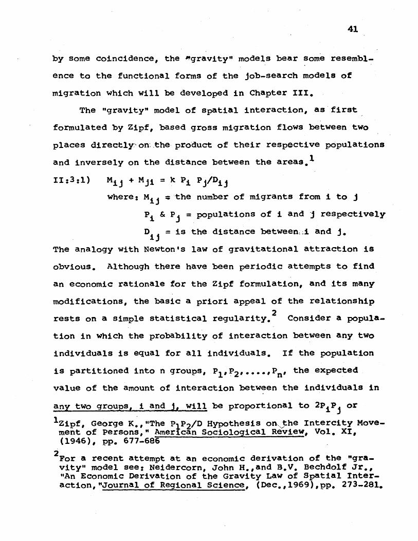
The "gravity" model of spatial interaction, as first
formulated by Zipf, based gross migration flows between two
places directly on'.the product of their respective populations
and inversely on the distance between the areas. 1
11:3:1) Mi + Mji = k Pi Pj/Dij
where: Mu 1 the number of migrants from i to j
P & P= populations of i and j respectively
D = is the distance betweenai and J.
The analogy with Newton's law of gravitational attraction is
obvious. Although there have been periodic attempts to find
an economic rationale for the Zipf formulation, and its many
modifications, the basic a priori appeal of the relationship
2rests on a simple statistical regularity. Consider a popula-.
tion in which the probability of interaction between any two
individuals is equal for all individuals. If the population
is partitioned into n groups, p ,P2'***** n, the expected
value of the amount of interaction between the individuals in
any two groups, i and j, will be proportional to 2 P PJ or
lZipf, George K., "The P P 2 /D Hypothesis onthe Intercity Move-.ment of Persons," AmerIcan Sociological Review, Vol. XI,(1946), pp. 677-686
2For a recent attempt at an economic derivation of the "gra-vity" model see: Neidercorn, John H.,and B.V. Bechdolf Jr.,"An Economic Derivation of the Gravity Law of Spatial Inter-action,"Journal of Regional Science, (Dec.,1969),pp. 273-281.
42
to a constant multiple of PP. of course if the partition
into groups is made on the basis of some factor that effects
the likelihood of interaction, such as distance between
individuals in the case of different city populations, that
factor would altter the expression for the expected value of
the level of interaction,
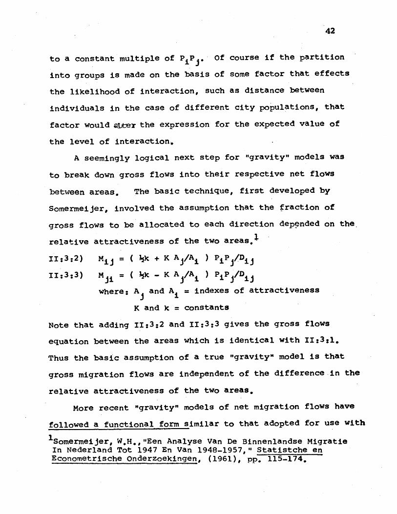
A seemingly logical next step for "gravity" models was
to break down gross flows into their respective net flows
between areas, The basic technique, first developed by
Somermeijer, involved the assumption that the fraction of
gross flows to be allocated to each direction depended on the.
relative attractiveness of the two areas,
11:3:2) Mu = ( k + K Aj/Ai ) PiP /Dij
11:3:3) Mu = ( Ik - K A /A ) PiP /Dij
where: A and A = indexes of attractiveness
K and k = constants
Note that adding 11:3:2 and 11:3:3 gives the gross flows
equation between the areas which is identical with 11:3:1.
Thus the basic assumption of a true "gravity" model is that
gross migration flows are independent of the difference in the
relative attractiveness of the two areas,
More recent "gravity" models of net migration flows have
followed a functional form similar to that adopted for use with
1 Somermeijer, W.H.,"Een Analyse Van De Binnenlandse MigratieIn Nederland Tot 1947 En Van 1948-1957," Statistche enEconometrische Onderzoekingen, (1961), pp, 115-174,
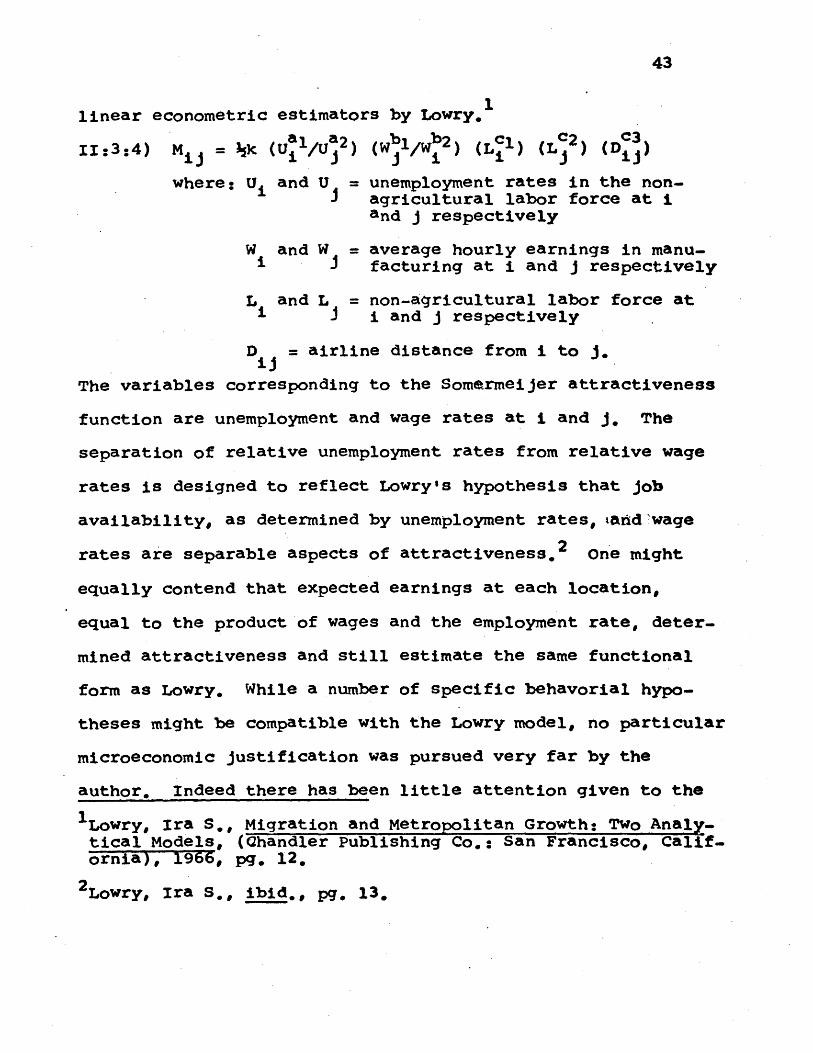
43
linear econometric estimators by Lowry.
11:3:4) Mu = k (Ual/Ua2) (W bl b2) (Lei) (L 2 ) (D3)
where: U and U = unemployment rates in the non-J agricultural labor force at i
and j respectively
W and W = average hourly earnings in manu-facturing at i and j respectively
L and L = non-agricultural labor force ati and j respectively
D = airline distance from i to J.
The variables corresponding to the Somermeijer attractiveness
function are unemployment and wage rates at i and J. The
separation of relative unemployment rates from relative wage
rates is designed to reflect Lowry's hypothesis that job
availability, as determined by unemployment rates, tarid wage
rates are separable aspects of attractiveness.2 One might
equally contend that expected earnings at each location,
equal to the product of wages and the employment rate, deter-
mined attractiveness and still estimate the same functional
form as Lowry. While a number of specific behavorial hypo-
theses might be compatible with the Lowry model, no particular
microeconomic justification was pursued very far by the
author. Indeed there has been little attention given to the
1 Lowry, Ira S., Migration and Metropolitan Growth: Two Analy-tical Models, (Chandler Publishing Co.: San Francisco, Calif.ornia), 1966, pg. 12,
2 Lowry, Ira S., ibid., pg. 13.
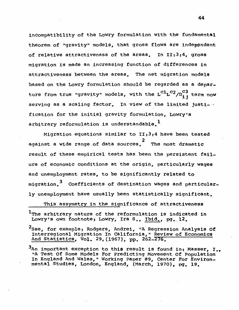
44
incompatibility of the Lowry formulation with the fundamental
theorem of "gravity" models, that gross flows are indeppndent
of relative attractiveness of the areas. In 11:3:4, gross
migration is made an .increasing function of differences in
attractiveness between the areas. The net migration models
based on the Lowry formulation should be regarded as a depar-
ture from true "gravity" models, with the LclLc2/Dc term now
serving as a scaling factor. In view of the limited justi-. -
fication for the initial gravity formulation, Lowry's
arbitrary reformulation is understandable.1
Migration equations similar to 11:3:4 have been tested2
against a wide range of data sources. The most dramatic
result of these empirical tests has been the persistent fail-
ure of economic conditions at the origin, particularly wages
and unemployment rates, to be significantly related to
migration.3 Coefficients of destination wages and particular-
ly unemployment have usually been statistically significant.
This assymetry in the significance of attractiveness
1The arbitrary nature of the reformulation is indicated inLowry's own footnote: Lowry, Ira S., Ibid., pg..12,
2See, for example: Rodgers, Andrei, "A Regression Analysis OfInterregional Migration In California," Review of EconomicsAnd Statistics, Vol. 29, (1967), pp. 262-276.
3An important exception to this result is found in: Masser, I.,"A Test Of Some Models For Predicting Movement Of PopulationIn England And Wales," Working Paper #9, Center For Environ-mental Studies, London, England, (March, 1970), pg. 19.
45
indexes at the origin and destination arises out of a depar-
ture from the spirit of the "gravity" model relationship.
Equations 11:3:2 and 11:3:3 suggest that population flows in
each direction depend on the relative attractiveness of the
two areas, and not on the absolute levels of attractiveness.
This suggests that the coefficients of wages and unemployment
be constrained to be equal, b1 = b2 and a1 = a2* Indeed
unless such a relationship is adopted the implied fofmule..
tibn suggests that migration increases with a rise in wages
or fall in unemployment rates. Lowry does report, in a foot-
note, that he tested a relative attractiveness formulation
and found it insignificant before moving on to his final
equation.1 Such trial-and-error approaches are not likely to
yield meaningful results.
In view of this wholesale rejection of the a priori
information in equations II:3:1 and 11:3:2, one might say
that the Lowry model, and its many derivitives, are more
noted for their departures from than their application of
the implications of the "gravity" model. The essentially
arbitrary or accidental nature of these quasi-gravity models
should be recognized when drawing inferences from estimated
values of their parameters.
A second problem that has been most troublesome to users
1 Lowry, Ira, ibid., pg. 13
46
of the Lowry formulation has been the possibility of simul-
taneous equation bias. This is particularly important in the
case of unemployment rates where migrat6n directly affects
the size of the labor force, one of the arguments of the
function determining unemployment rates. It is most difficult
to accept unemployment as an exogeneous variable. This sus-
picion is reinforced by empirical studies based on data from
California and the United Kingdom which showed that the
coefficient of destination unemployment, while statistically
significant, had the wrong sign, b was positive.
There is some precedent for assuming wages to be exog-
eneous in a migration equation. The argument is based on a
job-rationing model of the labor force. Money wages are
assumed to be inflexible in the short-run. Any excess supply
of labor in each location must then adjust to preserve unemp-
loyment rate differentials among labor market areas. Employ-
ment changes at various locations are exogeneous responses to
changes in demand or investment or technology or prices of
non-labor inputs. The extreme statement of the job-rationing
model, developed by Cicely Blanco, relates migration during a
time period to the unemployment rate implied by the difference
between unemployment at the conclusion of the time period and
the projected size of the work force due to natural increase
1 See, for results from California, Rogers, Andrei, op. cit.,pg. 265, and for results from the United Kingdom, Masser, I.,_. cit., pg. 19.
47
at the end of the time period.
11:3:5) NMt = a + b (EtLt) +b 2 (Et-1Lt-)
where: NM = net migration during the time period
Et = employment at the end of the time period
L = labor force at the end of the time per-t iod based on natural increase with no
migration
Et-1 = initial employment level
Lt-1 = initial labor force.
A number of variations of this model have been developed.2
The basic functional form suffers from additional problems
that are discussed in appendix II-A at the end of this
chapter. The assumption of wage rigidities and job-rationing
may be reasonable for one or perhaps even the five year period
required for the Lowry model, But this is an empirical ques-
tion and must be regarded as extremely suspect when applied
to models of migration flows over a decade as in much of this
literature.
Actually an elaborate rationalization for the absence of
a relationship between wage changes and employment, and hence
for the job-rationing model, was developed for long-run models.
Most interesting is the hypothesis of Borts and Stein that
1 Blanco, Cicely, "Prospective Unemployment.and InterstatePopulation Movements," Review of Economics and Statictics(May, 1964), pp. 221 and 222.
2 For example, see: Mazek, Warren,"Unemployment and theEfficacy of Migration," Journal of Regional Science, Vol. 9,No. 1,(April, 1969), pp. 101-107.
48
the demand for labor in particular labor markets is perfectly
elastic.I The basic driving force of economic growth in a
local area is assumed to be provided by industries selling in
a national market. The demand curve facing these export base
industries is assumed to be perfectly elastic at prevailing
national price levels since any one city supplies only a
small fraction of national output. Then, assuming elastic
supplies of capital and other non-labor inputs, and constant
returns to scale, the demand for labor will be highly elastic.
In such a world, net migration or any other force shifting the
supply of labor schedule affects employment and output of the
area but not wages. This is a long-run argument for job-
rationing models, with a reversed causality in which migration
determines employment and output.
One flaw in the Borts and Stein hypothesis lies in the
assumption of highly elastic demand for exports. For many
cities, export industries do provide a large fraction of nat-
ional demand.2 Also in a world of positive transportation
costs every plant and every city will face a downward sloping
demand curve reflecting the hhdrizontal summation of demand
curves at increasingly distant points. This is a fundamental
result of spatial pricing models,
1 Borts, George, and Jerome Stein, _. cit., pp. 210-220.
2 The classic demonstration of this point is' found in: Licht-enberg, Robert M.,One-Tenth of a Nation, (Cambridge, Massach-usetts: Harvard University Press), 1960, pp. 265-268.
49
The Borts and Stein hypothesis along with recent attempts
to test it in simultaneous equation models is the subject of
detailed analysis in Chapter IV:4. There it is shown that
the interaction between aggregation and simultaneous equation
problems virtually precludes estimation and identification of
the demand for labor curve given present data sources.
The literature on migration reviewed thus far suggests
two conclusions for furthur research, First additional general-
izations drawn from empirical regularities are not needed. Too
many results of this sort already exist and they tend to be
contradictory. The extreme statement of this contradiction is
seen in the assumption of perfectly elastic labor supply made
in the job-rationing literature and the assumption of perfectly
elastic demand for labor in the Borts and Stein models. Our
understanding of migration has advanced little since Raven-
stein's work. Secondly any attempt to build a microeconomics
of migration must reconcile contradictions in the literature
and account for empirical results from both the survey
research and econometric model literature. The next chapters
attempt such a formulation.
50
APPENDIX TO CHAPTER II
Most models of migration have related numbers of migrants
to the relative attractiveness of origin and destination areas
as indicated by wages, climate, unemployment, etc. Not only
have most of these formulations had little analytical content,
but the majority have even ignored basic desirable properties
which any migration function should have, one such property
is that when two areas are equally attractive there should be
no net flow of migrants between them. Any careful formulation
should take into account this piece of a priori information,
yet most migration functions in the literature do not.
The most common functional form for migration equations
has related the fraction of the -population at a particular
origin that migrated in a given time period to the attractive-
ness or relative attractiveness of that area and a given
destination. But this formulation, however desirable on other
criteria, is inconsistent with the desirable property that
equal attractiveness in both areas produce zero net migration.
Consider a world in which all areas are equally attrac-
tive. Interpreting this to mean that the fraction of total
population in any area migrating in a given time period is
equal for all areas, gives:
II:A:1) Mij/Ni = zi Z
where: Mij migrants from i to destination j
N = population of .area i
51
Z'.= fraction of population at i thatmigrates to j
z = fraction of population at i that migratesto any of the equally attractive destin-ations.
Similarly, using analogous notation to that in II:A:1, the
number of migrants from j to i is:
II:A:2) M IN = X J X
Now it has been agreed that if both areas are equally attrac-
tive net migration should be zero. This does not, however,
imply that zj ' z or that x = x or that z = x , as
is implied by most migration equations. Indeed zero net
migration requires that the fraction of migrants from differ-
ent areas be unequal. Consider the situation in which i and
j have equal migration flows in each direction.
IIA:3) M -M = Zx Nij Mi O= i N±i 0 ii jClearly in this instance of zero net migration the fraction
of out-migration from each area depends on the population
ratios of the two areas,
II:A:4) Z /x = N /N
Only if both areas have identical population .does zero net
migration imply equal probability of out-migration from both
areas,
Thus if all areas are equally attractive and there is
no net migration the fraction of out-migration from areas
with relatively large population will be small than that for

52
areas with small population.
53
CHAPTER III
A JOB-SEARCH MODEL OF MIGRATION
This chapter developes a job-search model of migration
among metropolitan areas. The model is based on concepts
first described in the literature on the economics of infor-
mation. This literature is surveyed first and the special
applicability of the economics of information to migration,
as opposed to other labor market applications commonly refered
to as the job-search models. Subsequent sections will build
a microeconomics of migration, both in terms of decisions by
workers and behavior of employers,
I11:1) The Economics Of Information And Job Search
The first attempts to formulate an economics of infor-
mation as a formal part of microeconomic theory are generally
1credited to George Stigler. In formulating an economics of
information, Stigler's first step was to note that positive
costs of search to both buyers and sellers implied that a
traditional pareto optimal market-clearing solution was the
exception.rather than the rule in real-world markets. Econo-
mic actors engage in recontracting and search only to the
extent that the marginal return to such activities exceeds
the marginal cost. This accounts for the distribution of
Stigler, George, "The Ecan6mics of Information, "1 Journal ofPolitical Economy, (June, 1961), pp. 211-225,
54
of prices that are commonly observed for identical goods and
services. Thus buyers cannot be expected to search out the
lowest price offered by any seller.
Given that they face distributions of bid (asked) prices,
sellers (buyers) can expect that, for most distributions,
there will be diminishing returns to search. The expected
value of maximum (minimum) price found by sellers (buyers)
increases (decreases) at a diminishing rate with additional
search efforts. Much emphasis has been placed on this margin-
al benefit from search function while the marginal search cost
function has been neglected. In general investigators have
had models of a single buyer or seller engaged in personal
examination of successive possible transactions. The average
cost per opportunity searched is usually assumed constant or
slightly increasing if the most convenient opportunities are
searched first. However, it is possible that due to learn-
ing effects involved in the search process the average cost
per search may decrease over a wide range. Several recent
articles have explored the extent of search expected of
workers by simulating markets subject to given price distri-
butions and search cost functions.1 The major result of
these efforts has been to show that only a very limited
lSee, for example: Gastwirth Joseph L.,"On ProbabilisticModels Of Consumer Search For Information," Working Paper;Harvard University, (June, 1971)
55
amount of search can be expected in most cases, and for most
goods.
Presently there has been no development of general
equilibrium analysis of an economy with positive search
costs. Indeed there has been little work on a theory of
consumer's demand in which prices of all goods are stochastic,
and information is costly. Unfortunately migration does
involve such a choice among many goods since the decision to
locate in a particular area is analogous to the choice among
commodities. Similarly information on wages is analogous to
information on prices, both being stochastic variables.
Clearly the way to preserve the notion of pareto optimal-
ity and its welfare implications in a market with positive
search costs and uncertain prices is to consider search as an
economic activity. This means that there will no longer be a
single price for homogeneous goods that clears the market but
a distribution of prices, Presumably the variance of the
distribution of prices for a particular good varies directly
with the cost of search. In the extreme cases of zero and
infinite search costs, prices become perfectly deterministic
and undetermined respectively. Unfortunately relatively few
other results on search costs and price distributions have
56.
been developed. If the only result of the economics of
information were to account for the observation that the
market price of homogeneous goods is not uniform, it would
amount to little more than a footnote to deterministic
microeconomic models.
The most interesting applications of the economics of
information have been in the form of job-search models of
labor market behavior. Job-search is the activity of gaining
information about employment activities, optimal search
calls for workers to examine successive job opportunities
with an wage criterion in mind. The first analysis of infor-
mation in the labor market was made by George Stigler. Most
of his results were analogous to those mentioned above for
the general economics of information. The dispersion of wage
offers was related directly to search costs both in theory
and in limited empirical tests. Also concrete expressions
for the marginal benefit from additional search were developed
for given wage distributions. The marginal benefit from add-
itional search is equal to the expected value of the increase
in whe maximum wage found when total searches are increased.
One optimal decision rule for workers in such a labor market
involves formulation of an acceptance wage by each worker
IStigler, George, "Information in the Labor Market," Journalof Political Economy, (October, 1962), pp. 94-105.
2 Stigler, George, ibid., pg, 97.
57
which represents the wage at which he will take a job and
cease search. Generally speaking the acceptance wage is
determined by finding the wage level at which the expected
value of additional wage increases is less than the costs
associated with additional search.
At least three features of the search process are vital
to the formulation of an acceptance wage, and to the nature
of the resulting job-search model. First is the question of
offer stockpiling. Can the worker retain an offer while he
searches furthur, or must an immediate decision be made?
Secondly the worker's knowledge of the actual distribution of
wages is important. The search process yields information on
the distribution being sampled. If knowledge of the actual
distribution is meagre, search activity may also cause the
estimate of this distribution to change. Under such circum-
stances, the properties of the acceptance wage become most
complex, as is so often the case when learning processes are
modeled. Third is the possibility of workers resampling
firms. Even if no openings were available at a particular
firm, the applicant should become aware -of the prevailing
wages and working conditions. If the search period were
rather long, workers might resample firms whose wages were
relatively high but which, temporarily, had no vacancies,
1Some attempts to deal with this problem are found in:Salop,S.C., "Systematic Job Search And Unemployment,"Working Paper,Yale University Theory Workshop, undated.
58
Any job-search model must make. some strong assumptions about
the characteristics of job offers reviewed above,
One additional modification of the job-search model
has caused it to assume its present prominence in the recent
literature. The cost of search is assumed to be higher for
employed than for unemployed individuals. Thus unemployed
workers will decline job offers that are above the level of
unemployment compensation that they could recetve while out
of work because accepting such employment, even on a tempor-
ary basis, could interfere with furthur search. Such behavior
places the unemployed in a different light. The Bureau of
Labor Statistics has long defined unemployed workers as those
who indicate that they attempted to find work without success
during the past week. The job-search formulation implies
that these workers are engaged in useful economic activity,
trying to place their human capital in its highest use. Their
present status reflects a desire to continue high levels of
search activity rather than be constrained by a job. Workers
who perceive the distribution of wages to be higher than its
actual level will tend to be recorded as unemployed for long
periods. To a certain extent, the observation of high levels
of job vacancies accompanying sizable unemployment may reflect
the divergence of expectations and actual wages prevailing.
59
Unfortunately there is relatively little empirical
evidence on the relative ,costs of job search for those
employed and unemployed. Survey research results reviewed
in Chapter 1':3 suggest that few unemployed workers actually
refuse a concrete job offer and that their reservation wage
is about 25% below the average wage actually accepted. If
relative search costs for the employed really interfered with
job-search, more unemployed workers would turn down jobs and
wages actually accepted would approximate reservation wages.
What is even more disturbing in most job-search models of
unemploy!tent and wage changes is the implicit assumption in
many models that continued search while employed is virtually
precluded by costs or other aspects of the search decision.
This assumption often creeps into job-search models indirectly.
The acceptance wage is found by solving for the offer which
equates marginal costs of immediate search efforts with the
present value of marginal expected gains from search. Present
values of benefits are computed by discounting over the number
of years until retirement. At a time in which one in three
marriages ends in divorce and the sum of accessions and sep-
arations per year equals half the size of the labor force, it
seems rather nAlve for workers to discount values over long
periods of time. Surely in many cases workers take jobs with
the prospect of furthur search. In many cases, the accession
1 Chapter 1:3 reviewed survey results showing accepted wages25% above reservation wages.

60
is viewed as temporary by both the employer and employee.
In addition to the information presented above, survey
research results are available on characteristics of local
labor market search on the part of unemployed workers. Rec-
ently unemployed workers apparently concentrate their search
effort shortly after job separation. After the first week
of unemployment, the rate of search falls to one or two oppor-
tunities per week for the average worker. It is difficult
to believe that employment for toxrty hours per week could
preclude such levels of activity, let alone part time employ-
ment.
Thus it is not obvious that the economics of information
can be applied meaningfully to labor market activity. Past
job-search models of local labor market activity have made
strong assumptions concerning relative search costs when
employed and unemployed and expected duration of employment.,
Both these assumptions appear to be in conflict with the
limited empirical evidence available. The vast majority of
job-search models appear to ignore these conflicts.2 This
will not be the case with the job-search model of migration
developed here. Indeed the migration decision will be shown
to be particularly well suited to a modified model based on
the economics of information,
1 Sheppard, Harold, and Harvey Belitsky, The Job Hunt, (Balti-.moreMaryland:Johns Hopkins Press), 1966, pg. 55.
2 See, for example: Mortensen;Dale "Job Search And Unemploy-ment, "American Economic Review, ( July, 1970), pp. 847-861.
61
II:2) Migration And The Economics Of Information
The previous section catalogued a number of areas in
which assumptions about the relationship between workers and
job opportunities must be made in order to apply job-search
models to particular labor market situations, Most important
is the duration and durability of job acceptances. This issue
will be considered first in relation to the migration decision
to be modeled here,
Migration differs from the ordinary local labor market
job acceptance decision, Previously the assumption that job-
search activity was significantly constrained by employment was
questioned. The decision to accept a job is not equivalent to
nor does it imply a decision to cease search, However migra-
tion is costly, Both out-of-pocket moving costs and implicit
social and psychological costs of changing location are invol-
ved in the migration decision. Although return flows of mig-
rants are large, it would appear that migrants do regard the
decision to accept a job at a distant location as a relatively
long-run decision. In addition, job-search at a distance is
costly, often involving special trips. Moving to a different
labor market area means trading one set of local job opportuni-
ties for a new set, Obviously this does not guarantee that
all future search will be concentrated at the destination, But,
since the relative costs of search have been altered, certainly
62
the relative importance of the origin as a locus of search
will be diminished.
Both the large transactions costs involved in fnoving and
the change in relative search costs at the new location, indic-
ate that the migration decision implies a long-run commitment
to participate in the destination labor market. This result
holds even if the worker exchanges unemployment at the origin
for similar labor fcrce status at the destination. Such moves
are based on individual perceptions of the long-run return to
search at different locations. This is consistent with
the implicit assumption in job-search models that the job
acceptance decision involves long-term comparisons and term-
ination of search.
A number of other aspects of the employment decision were
presented in the previous section as being critical to the
application of the economics of information to labor market
decisions. First was the question of offer stockpiling. It
would seem that in the case ot job offers at a distance some
degree of negotiation and/or opportunity for consideration over
time would be allowed by employers. Under these circumstances
some offer stockpiling is possible.
Secondly there is a question of the degree of learning on
the part of job searchers. Specifically learning involves
63
changes in a worker's perception of the actual distribution
of wages as a result of search. Surveys of workers indicate
that perceptions of wage levels and reservation wages are
rather insensitive to the degree of search.' There is a
fundamental difficulty involved in analyzing learning phenomena
in a static equilibrium-model. Presumably search causes the
perceived wage distribution to approach the actual distribution.
In dynamic models with changing wage rates it is possible to
model this process. But in static models or equilibrium models,
it is difficult to account for or describe the nature of any
divergence of actual and perceived wages. Thus for static or
equilibrium models of the sort that will be developed here the
actual wage distribution will be assumed to be identical to
2the expected distribution. No learning occurs during the
search process. It may be that static models are less approp-
riate than dynamic models. Thus if origin wages are changing
quickly there may be a significant difference in current and
expected wages. Such expectations phenomena would be greatest
at the origin because workers there have presumably experienced3
wage changes over time.
Kasper, H.,"The Asking Price Of Labor And The Duration Of Unemp-loyment," Review of Economics And Statistics,(May,1967), pg.145
2If there were any difference between actual and expected wages,search processes would logically modify worker expectations,
3Dynamic models might show why origin wages have often provedinsignificant in empirical studies. But the simultaneity bet-ween wage changes and migration would cloud the results obtain-ed from any crossection data.

64
A third consideration is the possibility of resampling
firms which had no appropriate vacancies when initially
searched. This would appear to be an important phenomenon
in local labor markets where many workers find employment
through recalls or returning to places of previous employment.
Recall or resampling on the basis of position on a waiting list
would appear to be less likely when worker residence is distant
from the firm. Unless a firm, which presently has no vacancies,
anticipates an immanent change in workforce requirements, it
will tend to confine its recall and job application files to
local residents. Thus all search efforts at a distance will
be regarded as new sampling or job-search efforts.
There are a number of questions that have particular
relevence to the attempt to apply the economics of information
to migration that do not arise in ordinary job-search models.
Perhaps the most important difference in the migration decision
is that workers are sampling from many wage distributions, each
at a different location with its own search costs. If the
migration decision is based only on wages, workers who were
fully aware of the distribution of wages everywhere would only
search for opportunities at one location. This does not imply
that all search will be at a single destination because search
costs will vary among individuals, even at a given location,
and of course moving costs will also vary with distance from a
65
given origin. The tendency to concentrate search in one area
when all wage distributions are known completely will be incre-
ased if the average cost of search decreases. The failure to
consider alternative destinations agrees well with survey1
research accounts of the migration decision. Unfortunately.
such assumptions of complete knowledge of wages are difficult
to model analytically. The greatest difficulty can be seen
by noting that the reservation wage of workers at one location
bears no necessary relationship to the actual wages observed
there. Reservation wages at any origin would be a weighted
average of reservation wages based on wage distributions and
search at a variety of alternative locations.
There are two obvious drawbacks or contradictions in
assumptions of knowledge of wages elsewhere. First survey
research suggests that most workers are only dimly acquainted
with wages in the local labor market.2 Job opportunities at
more distant locations should prove even more obscure. Secondly
search patterns of local workers, primarily the unemployed,
indicate that the vast majority of search effort is concentrated
within a metropolitan area. Few, if any, workers search more
intensively at a distance than they do in the local labor market.
1 This result was presented in Chapter 1:3. A majority ofworkers report considering no alternative destinations.
2 For example, see: Parnes, HerbertResearch On Labor Mobility
o2. cit.0 pg. 78.

66
A rpore realistic assumption concerning the degree of
knowledge about wage distributions is that workers only have
accurate information on prevailing wages in their local labor
market. Indeed survey research evidence indicates that worker
knowledge of local labor market conditions is often poor,
1lacking both precision and accuracy. Under these circumstan.
ces the reservation wage for all workers within a labor market
will be based on the distribution of wages and search costs
in the metropolitan area. There will be a range or distribu-
tion of reservation wages even if all workers at a location
know wages precisely, due to differences in worker attributes,
and variations in search costs and present wages of employed
workers.2
The mechanism of the migration decision operates to keep
workers ignorant of opportunities elsewhere. If the reserva.
tion wage is based on local labor market conditions, then the
individual who examines opportunities elsewhere will quickly
reach one of two conclusions. Either he will find wages lower
than those at the origin and terminate search or he will accept
the first offer above his reservation wage. In this second
case migration follows and search efforts are concentrated in
1 For an example showing that workers in lowest wage firms sawtheir wages near the median for the metropolitan area see:Parnes, Herbert, ibid., pg. 78,
2Thus even abstracting from differences in worker attributes,age, sex, skill, etc., reservation wages will differ,
67
the destination. Workers, having found an attractive offer
elsewhere, cannot be expected to remain long in their initial
location.
A second complication in applying the economics of irifor-
mation to the migration decision arises because choice of job
and residential location is compounded. For most workers
consumption is necessarily tied to the area in which they are
employed. Migration involves a comparison of real wages defin-
ed in their most comprehensive sense. For this reason equili-
librium in a system of labor markets does not even imply equal-
ity of wages adjusted for differences in cost of living.
Differences in general amenity among areas, such as aspects of
scenery, or climate, will cause equilibrium wages adjusted for
the cost of living to diverge. Henceforth the term attractiveo.
ness will be used to refer to the composite of wages, cost of
living, and amenity that characterizes an area.
A final pecularity of the migration decision that affects
direct application of the economics of information is the
tendency of firms to bear a portion of search costs. Almost
40% of migrants who reported that they moved for economic
reasons found their position through an employer's represen-.
tative. of course, employers often assume a portion of search
1Lansing, John and Eva Mueller, The Geographic Mobility Of Labor(Ann Arbor, Michigan: University of Michigan Press), 1967,pg. 231.
68
costs within local labor markets, but this labor market
phenomenon has not been included in job-search models thus
far.
It might seem that employer-financed search would be
concentrated in local labor markets. Firms can be expected to
search most intensively in areas where the return to search is
high. There are regional disparities in wages paid for similar
work. There is some doubt of the ability of employers to cap-
italize on these wage differentials by paying migrants lower
wages. Unions enforce uniform wage scales.2 Even if these
schedules can be avoided by changing job qualifications, firms
paying low wages will experience high turnover rates. Once a
worker has moved to a new job market he should quickly adjust
to new wage rates. Unless there are barriers to labor mobility
in the local labor market, newly arrived workers should soon
demand the same level of compensation as others similarly
situated in the local market. Cases in which massive labor
importation has occured usually accompany barriers of race,
ethnicity, language, etc. that keep new arrivals out of the
local labor market. 3 Recent evidence of bounty payments for
ISee the discussion in Chapter 1:2.
2 See, for example: Rees, Albert, and Schultze, George, WorkersAnd Wages In An Urban Labor Market,(Chicago, Ill.: Universityof Chicago Press), 1970, Chapter 4.3Involuntary servitude was an extreme case of the attempt toinsure that employers could capitalize on search costs invol-ved in recruiting low wage labor from distant markets.
69
Mexican migrants to the United States and African migrants to
France indicate that this crude form of employer search is
still prevalent.
Obviously none of the barriers mentioned above apply to
migrants between metropolitan areas in the United States. But
an incentive for employer search at a distance still remains.
Although for a given expenditure more applicants can probably
be searched by concentrating search on the local labor market,
the return from search depends on the number of acceptances
that given search experiditure can achieve. For a given wage
offered by the firm, the number of acceptances from given
applicants will vary inversely with the expected value of the
acceptance wage at a particular location. Even if the number
of applications per dollar of expenditure on search is larger
at nearby locations, firms will engage in distant search if
acceptances per application are sufficiently likely elsewhere.
Obviously there is a simultaneous relationship between wages
offered and search costs. As it becomes difficult to gain
the required number of accessions from the local labor market,
firms will raise wages in order to lower search costs and
other costs related to turnover rates. Since relative search
1For a recent example indicating that French employers paya bounty equivalent to $300 for each African worker smuggled
into France, see: Larrimore, Don M., "Ring Said To HaveSmuggled Thousands Into France, " The Washington Post, (July,20, 1972), pg. A21.
70
costs are important in determining the pattern of worker
search effort, it is important to consider possibilities for
employer search at a distance in formulating any model of
migration.
The assumptions discussed above, and often neglected in
analyzing labor market behavior, will have an important effect
on the models of migration developed here.
111:3) Model of Migration And Worker's Job Search
This section will develop a model of migration based on
the economics of information, and concerned directly with the
worker's labor market choice. First assumptions of the model
are reviewed. Then the conditions for optimal search are
developed, subject to different assumptions concerning know4.
ledge of wages elsewhere.
The attempt here is to account for job search behavior on
the part of homogeneous labor at one location in response to
homogeneous job vacancies at a variety of locations. As was
discussed in the previous section, workers can engage in offer
stockpiling. The time required to search additional opportun-.
ities is short compared to the decision time required by employ-
ers between initial application and final acceptance. No
learning occurs in the search process. Worker perceptions of
prevailing wage distributions are not significantly modified as
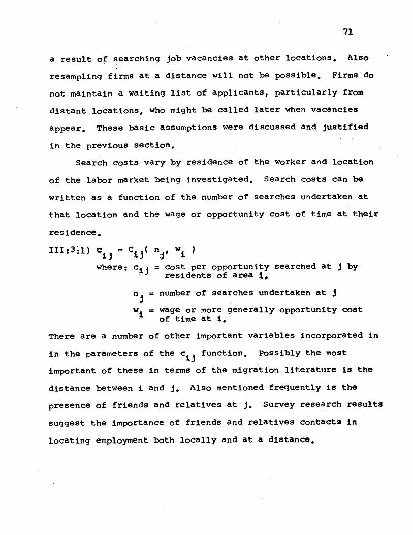
71
a result of searching job vacancies at other locations. Also
resampling firms at a distance will not be possible. Firms do
not maintain a waiting list of applicants, particularly from
distant locations, who might be called later when vacancies
appear. These basic assumptions were discussed and justified
in the previous section,
Search costs vary by residence of the worker and location
of the labor market being investigated. Search costs can be
written as a function of the number of searches undertaken at
that location and the wage or opportunity cost of time at their
residence.
III:31i) c = C ( n, w
where: Cj = cost per opportunity searched at j byresidents of area t,
n = number of searches undertaken at j
w = wage or more generally opportunity costof time at i.
There are a number of other important variables incorporated in
in the parameters of the c function. Possibly the most
important of these in terms of the migration literature is the
distance between i and j. Also mentioned frequently is the
presence of friends and relatives at j. Survey research results
suggest the importance of friends and relatives contacts in
locating employment both locally and at a distance.
72
Workers are assumed to allocate their labor services and
search activities so as to maximize their wealth, or the
rate of return on their human capital, subject to consumption
effects mentioned above. The consumption effects, other than
relative prices which are embodied in real wages, are embodied
in what will be called an attractiveness function.
III:3:2) a = A ( G *..... Gkj)
where: a = a value of attractiveness of area j interms of dollars per unit time,
G .... G = index of of each element oflj kj attractiveness at j, based on
climate, etc.
Because there are large moving or transaction costs associated
with migration, the worker is involved in a comparison of
flows of earnings at two different locations. The expected
value of this income flow confronting a worker in area i and
currently receiving a real wage of wj depends on the time until
retirement and the distribution of offered wages. If, for
ease of notation, the average time needed to search one job
opportunity is used as the basic measure of time, then it is
easy to show that a worker may spend the number.of time periods
remaining until retirement in three ways. First he may work
at i and not search any other location. Alternatively workers
may be employed or unemployed at i and actively engage in
search at other destinations. In this case search costs are
1Here retirement is equivalent to expected duration of job.
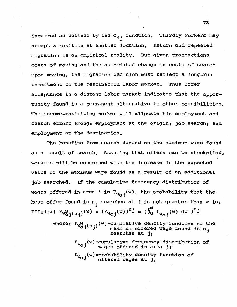
73
incurred as defined by the C function. Thirdly workers may
accept a position at another location. Return and repeated
migration is an empirical reality. But given transactions
costs of moving and the associated change in costs of search
upon moving, the migration decision must reflect a long-run
commitment to the destination labor market. Thus offer
acceptance in a distant labor market indicates that the oppor-
tunity found is a permanent alternative to other possibilities.
The income-maximizing worker will allocate his employment and
search effort among: employment at the origin7 job-search7 and
employment at the destination.
The benefits from search depend on the maximum wage found
as a result of search. Assuming that offers can be stockpiled,
workers will be concerned with the increase in the expected
value of the maximum wage foudd as a result of an additional
job searched. If the cumulative frequency distribution of
wages offered in area j is Fwoj(w), the probability that the
best offer found in n searches at j is not greater than w is:
III:3:3) Fwoj(nj)(w) = (Fwoj(w))n - ( w) dw )nj
where: FwM (w)=cumulative density function of thej'j) maximum offered wage found in njsearches at j1
F (w)=cumulative frequency distribution ofwoj wages offered in area j7
f (w) =probability density function ofoffered wages at j.
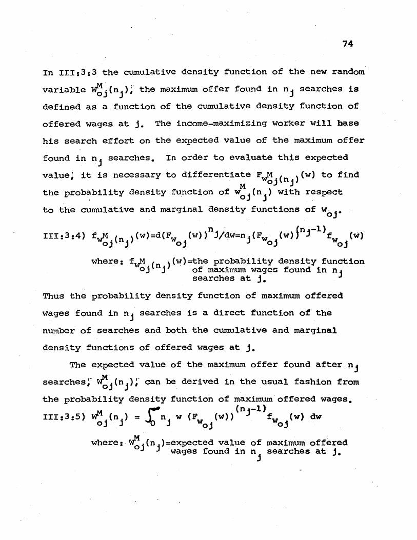
74
In 111:3:3 the cumulative density function of the new random
variable WM (n );- the maximum offer found in n searches isoj j
defined as a function of the cumulative density function of
offered wages at J. The income-maximizing worker will base
his search effort on the expected value of the maximum offer
found in n searches, In order to evaluate this expected
value, it is necessary to differentiate Fj(n) (w) to find
the probability density function of w (nj) with respect
to the cumulative and marginal density functions of w ,
111:3:4) fwM (n )(w)=d(Fw (w) )nJ/dw=n (F (w)ini)f (n-)
oj -j ojojoj
where: fwM (n )(w) =the probability density functionOj J of maximum wages found in n
searches at J.
Thus the probability density function of maximum offered
wages found in n searches is a direct function of the
number of searches and both the cumulative and marginal
density functions of offered wages at J.
The expected value of the maximum offer found after nj
searches; 7M (n ) can be derived in the usual fashion fromoJ j
the probability density function of maximum offered wages.
II:3:5) WM (n ) = n w (F (w)) f (w) dwoj j j w0j w)d
where: WM (n )=expected value of maximum offeredO0J J wages found in n searches at J.
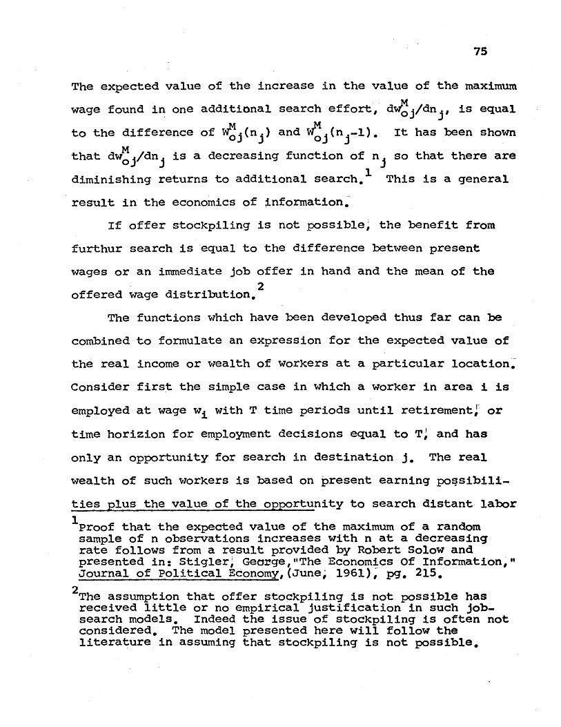
75
The expected value of the increase in the value of the maximum
wage found in one additional search effort, dwM /dnj, is equal
to the difference of WM.(n ) and W (n -1), It has been shown0) j oj j
Mthat dw0 /dn is a decreasing function of n so that there are
diminishing returns to additional search, This is a general
result in the economics of information.
If offer stockpiling is not possible; the benefit from
furthur search is equal to the difference between present
wages or an immediate job offer in hand and the mean of the
2offered wage distribution.
The functions which have been developed thus far can be
combined to formulate an expression for the expected value of
the real income or wealth of workers at a particular location.
Consider first the simple case in which a worker in area i is
employed at wage wj with T time periods until retirement, or
time horizion for employment decisions equal to T' and has
only an opportunity for search in destination j. The real
wealth of such workers is based on present earning possibili-
ties plus the value of the opportunity to search distant labor
%Proof that the expected value of the maximum of a randomsample of n observations increases with n at a decreasingrate follows from a result provided by Robert Solow andpresented in: Stigler, George,"The Economics Of Information,"Journal of Political Economy, (June, 1961), pg. 215,
2The assumption that offer stockpiling is not possible hasreceived little or no empirical justification in such job-search models, Indeed the issue of stockpiling is often notconsidered. The model presented here will follow theliterature in assuming that stockpiling is not possible,
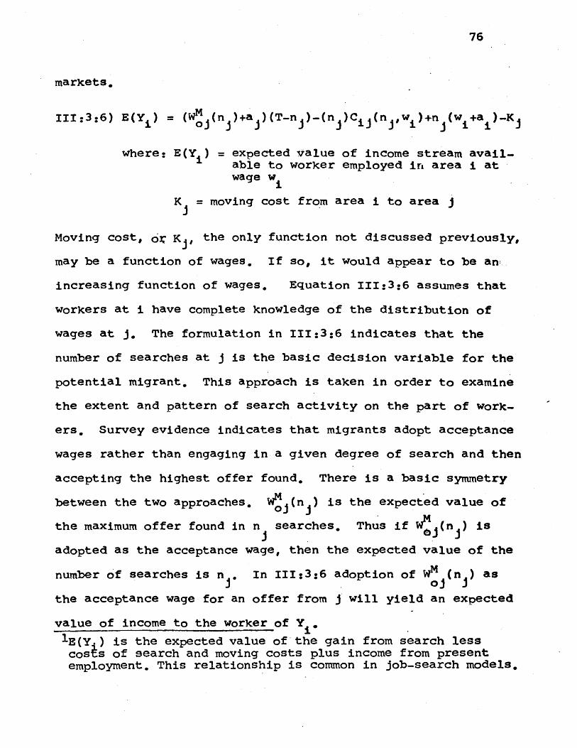
76
markets.
111:3:6) E(Y) = (WM (n )+a )(T-n )-(n )C (n ,w )+n (w +a )-K£oj j ijiij 'i i
where: E(Y ) = expected Value of income stream avail-able to worker employed in area i atwage w
K = moving cost from area i to area j
Moving cost, o K , the only function not discussed previously,
may be a function of wages. If so, it would appear to be an
increasing function of wages. Equation 111:3:6 assumes that
workers at i have complete knowledge of the distribution of
wages at j. The formulation in 111:3:6 indicates that the
number of searches at j is the basic decision variable for the
potential migrant. This approach is taken in order to examine
the extent and pattern of search activity on the part of work-
ers. Survey evidence indicates that migrants adopt acceptance
wages rather than engaging in a given degree of search and then
accepting the highest offer found. There is a basic symmetry
between the two approaches. WM (n ) is the expected value ofoj
the maximum offer found in n searches. Thus if (n is
adopted as the acceptance wage, then the expected value of the
number of searches is n In III:3:6 adoption of WM (n ) asO oj j
the acceptance wage for an offer from j will yield an expected
value of income to the worker of Y1E(Y ) is the expected value of the gain from search lesscosts of search and moving costs plus income from presentemployment. This relationship is common in job-search models.
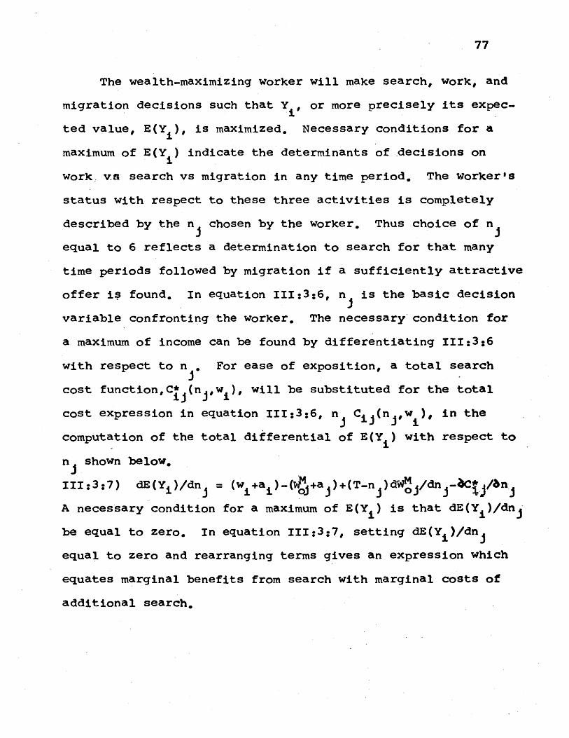
77
The wealth-maximizing worker will make search, work, and
migration decisions such that Y, or more precisely its expec-
ted value, E(Yi), is maximized. Necessary conditions for a
maximum of E(Y ) indicate the determinants of .decisions on
work, va search vs migration in any time period, The worker's
status with respect to these three activities is completely
described by the n chosen by the worker, Thus choice of n
equal to 6 reflects a determination to search for that many
time periods followed by migration if a sufficiently attractive
offer is found, In equation 111:3:6, n is the basic decision
variable confronting the worker. The necessary condition for
a maximum of income can be found by differentiating 111:3:6
with respect to n , For ease of exposition, a total search
cost functionC* (n ,w ), will be substituted for the total
cost expression in equation 111:3:6, n jC ij(n ,w), in the
computation of the total differential of E(Y ) with respect to
n shown below.
111:3:7) dE(Yi)/dn = (wi+a±)-( +a )+(T-n )dWI/dn -.C/
A necessary condition for a maximum of E(Y ) is that dE(Y )/dn
be equal to zero. In equation 111:3:7, setting dE(Y i)/dn
equal to zero and rearranging terms gives an expression which
equates marginal benefits from search with marginal costs of
additional search,
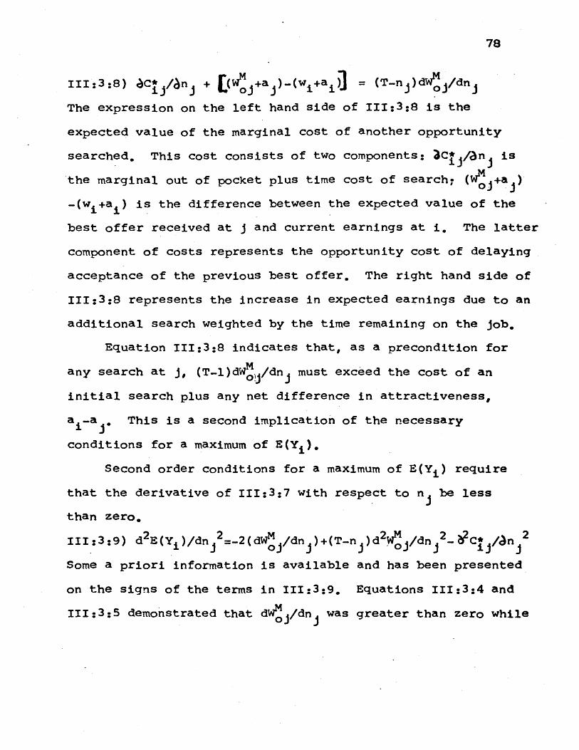
78
111:3:8) aC* /an + ( +a ).(w +a)] = (T-n )dWM/dniji +. Ewoj j ii j
The expression on the left hand side of 111:3:8 is the
expected value of the marginal cost of another opportunity
searched. This cost consists of two components: 3C*/3n is
the marginal out of pocket plus time cost of search7 (WM +a )
-(wi+ai) is the difference between the expected value of the
best offer received at j and current earnings at i. The latter
component of costs represents the opportunity cost of delaying
acceptance of the previous best offer. The right hand side of
111:3:8 represents the increase in expected earnings due to an
additional search weighted by the time remaining on the job.
Equation 111:3:8 indicates that, as a precondition for
any search at j, (T-1)dWM /dn must exceed the cost of an
initial search plus any net difference in attractiveness,
a i-a j. This is a second implication of the necessary
conditions for a maximum of E(Yi).
Second order conditions for a maximum of E(Yi) require
that the derivative of 111:3:7 with respect to n be less
than zero.
III:3:9) d2E(Yi)/dn 2 =-2(dW /dn )+(T-n )d2 /dn 2_?C* /cn 2
Some a priori information is available and has been presented
on the signs of the terms in 111:3:9. Equations 111:3:4 and
111:3:5 demonstrated that dW j/dn was greater than zero while
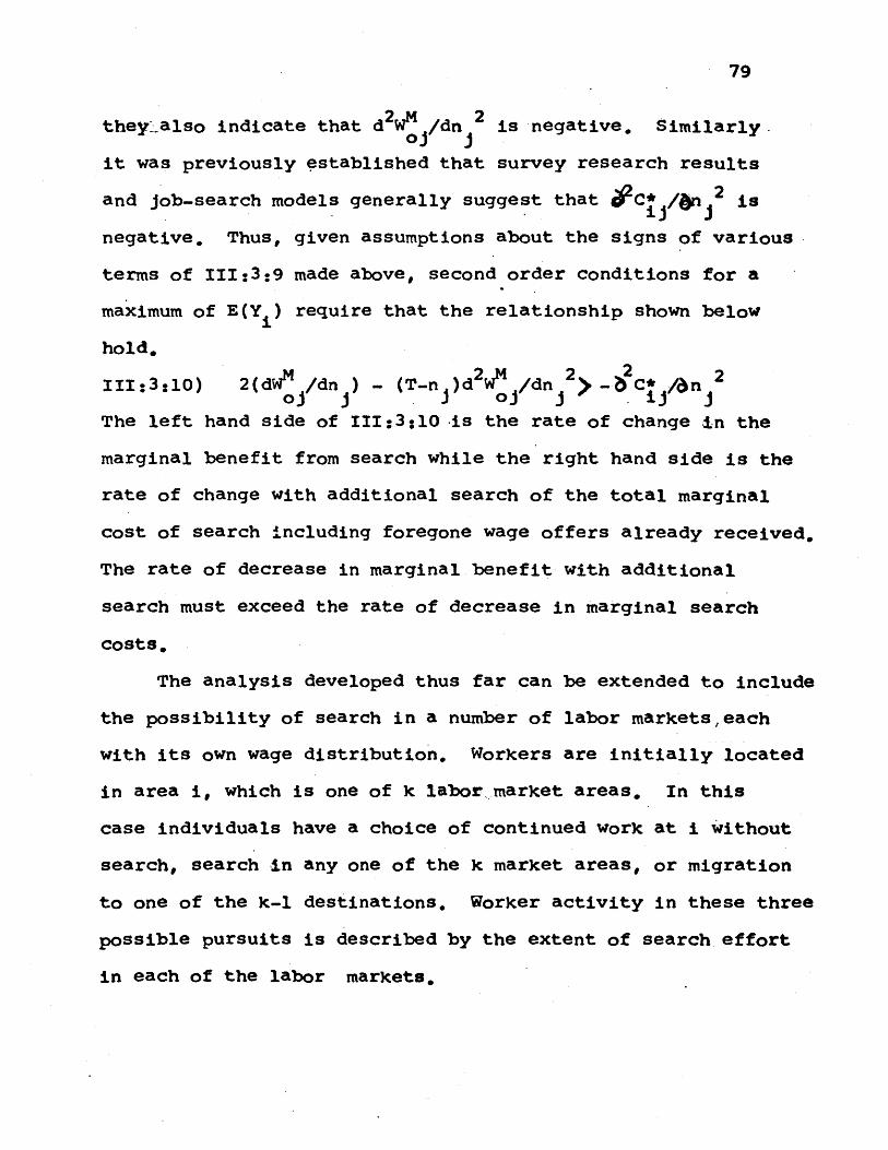
79
they also indicate that d2WM /dn 2 is negative. Similarly.oj j
it was previously established that survey research results
and job-search models generally suggest that eC* /45n 2 is
negative. Thus, given assumptions about the signs of various
terms of 111:3:9 made above, second order conditions for a
maximum of E(Y ) require that the relationship shown below
hold.
111:3:10) 2(dWM /dn ) - (T-n )d2 W /dn 2> C* /&n 2oj j i oj j ij j
The left hand side of 111:3:10 .is the rate of change in the
marginal benefit from search while the right hand side is the
rate of change with additional search of the total marginal
cost of search including foregone wage offers already received.
The rate of decrease in marginal benefit with additional
search must exceed the rate of decrease in marginal search
costs.
The analysis developed thus far can be extended to include
the possibility of search in a number of labor markets each
with its own wage distribution. Workers are initially located
in area i, which is one of k labor market areas. In this
case individuals have a choice of continued work at i without
search, search in any one of the k market areas, or migration
to one of the k-l destinations. Worker activity in these three
possible pursuits is described by the extent of search effort
in each of the labor markets.
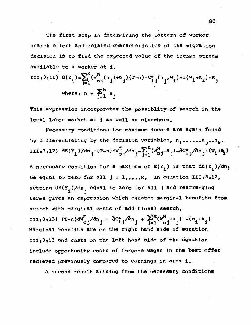
80
The first step in determining the pattern of worker
search effort and related characteristics of the migration
decision it to find the expected value of the income stream
available to a worker at i.
111:3:11) E(Y )=Z (o (n )+a )(T-n)-C* (n w )+n(w +a )-K
where: n = jk nj=l J
This expression incorporates the possiblity of search in the
local labor market at i as well as elsewhere.
Necessary conditions for maximum income are again found
by differentiating by the decision variables, n 1 .....n ..nk*
111:3:12) dE(Y )/dnj=(T-n)dWM /dn -k (WM +a )-bC* /bn +(w +ai i - oJ i=l oj 1 11 1:,
A necessary condition for a maximum of E(Yi) is that dE(Y i)/dnj
be equal to zero for all j = 1..,..k. In equation 111:3:12,
setting dE(Y )/dn equal to zero for all j and rearranging
terms gives an expression which equates marginal benefits from
search with marginal costs of additional search.
111:3:13) (T-.n)dWM /dn = ZC*/An + jk(WM +a ) -w +a )oj j ii j j=l oj j i i
Marginal benefits are on the right hand side of equation
111:3:13 and costs on the left hand side of the equation
include opportunity costs of forgone wages in the best offer
recieved previously compared to earnings in area i.
A second result arising from the necessary conditions
81
derived above is that the ratio of the expected value of
benefits to out of pocket search costs is the same for all
locations.
111:3:14) (T-n)dWM /dn _ (T-n)dWM,/dn, - (T-n)dW~k/dnk
CJ an ~ &Cgnn 3 ik/ nk
Equation 111:3:14 suggests the basic conditions for partition-
ing search among alternative locations. If a location is to
be searched at all, the ratio of the increase in the expected
value of the maximum wage offer found at that location to
marginal out of pocket search costs must equal the ratio at
other locations searched, Thus the increase in expected value
of maximum offered wages found per dollar of out of pocket
search cost must be equal at all locations searched,
The decision rule for migration and job search implied by
III:3:12 to 111:3:14 involves conducting n searches while
continuing employment at i, Searches are distributed among
the k destinations to satisfy the first order conditions in
111:3:14. The worker will then accept the offer whose w +a
is largest, An alternate decision rule involves establishing
a reservation or acceptance wage, In the case of the model
developed above, the reservation wage is equivalent to the
expected value of the maximum wage and attractiveness combina-
tion found in n searches, Thus the reservation wage which
82
would be consistent with this search model is based on a
weighted index of offered wage distributions elsewhere. The
weights are a function of the degree of search in each labor
market.
Another possibility for worker search is the absence of
significant information on wage distributions elsewhere. In
this case, there may be a tendency to assume that wages offer-
ed at a number of alternative locations are identical. Such
limited knowledge requires little modification of the model
which was developed for the case of perfect information.
There was no presumption in equation III:3:12 that the WM
functions were accurate or even that they were not identical.
However, if all offered wage distributions are identical -
perhaps believed to be the same as those at i - the a priori
results developed on the basis of first order conditions are
subject to more concrete interpretation. For example, in
equation 111:3:14, if offered wage distributions are identical,
the number of searches in each area actually searched depends
only on the shape of the C functions.
Second order conditions for a maximum of real income
require that d2E(Y )/dn 2 is less than zero. As was the case
when search at one alternate destination was considered, these
conditions require the rate of decrease in the expected value
83
of the maximum offer found at a given location exceed the
rate of decrease in total costs of search including foregone
earnings in the best position previously found.
111:3:15) -(T-n)d 2WM /dn 2 >2C / n 2 + dWM /dn + d /dnjoj i jinj dWidn oj 'i
The right hand side of 111:3:15 is the rate of change with
additional search of the total marginal cost of search includQ '
ing foregone wage offers already received. The left hand side
of this inequality reflects the rate of change of the expected
value of the best offer found.
The results presented thus far illustrate the rationale
for search at a number of alternative locations preceeding
migration. The number and pattern of locations searched
depend on characteristics of search costs and the extent of
knowledge of opportunities elsewhere.
IV 4) Recruiting Efforts By Employers
Survey responses of migrants reviewed in Chapter I1:3
indicate that search efforts on the part of employers are
important in providing information needed for or by migrants.
But a substantial portion of job-search literature and aLeo
the human capital models of migration neglect employer-finan-
ced search entirely. The rationale for this omission has
been that there is no economic return to employer search
84
outside the local labor market. Workers, who are induced to
move to a distant labor market, will quickly adjust to
prevailing wages at the destination.
Even if workers quickly adjust to local wages or local
restrictions and labor contracts fix wage levels for workers
of given skill, there remain-positive returns to search by
firms, Changing labor force requirements and separations, both
anticipated and unanticipated, imply that firms muse secure
a flow of new workers, These accessions come from recalls and
new hires based on applications for.positions vacant, Search
effort by the firm can increase the flow of applications recei-
ved, The fraction of acceptances from applications received
depends on the probability that offered wages are above the
reservation wage of applicants. This probability will be term-
ed the offer acceptance probability. While searching distant
labor markets may be more expensive than local search for
employers, offer acceptance probability may be higher at a
given wage offer in areas where reservation wages are lower,
This is the source of returns to employer search,
The remainder of this section will develop a simple model
of the extent and distribution of employer search activity in
a system of labor merkets, First firms at a particular loca-
tion can define a loss function related to vacancies. In an
abstract sense, such a loss function could be viewed as the
value of the marginal physical product of labor given differen
ces in the size of the workforce. The number of separations
85
is assumed to be forecast with certainty along with demand
for firm output. This means that the value of the marginal
physical product of labor can be determined and losses as a
function of vacancies unfilled can be represented for a firm
located in area j by L (v ). For the firm L (v ) will be the
difference between the prevailing level of offered wages,
which are only adjusted infrequently, and the value of the
marginal physical product of labor.
Optimal personnel policy for the firm described above
involves allocating funds to labor recruitment so that the
sum of L (v ) and recruiting costs is a minimum, Firms may
search at any one of k locations. They may recruit applicants
in various areas according to the simple cost function below.
III:4:1) rj = Rij(x)
where: r = total cost of recruiting applicants
x= number of applicants recruited fromarea i.
Probably the most important constant embodied in R is
distance from the firm to area i, size of i may be important.
Applicants can only be translated into vacancies filled
through a process of determining their abilities and finally
IFor an individual firm L (v ) depends on the price of outputy
prices of variable inputi other than labor; present size of
the labor force less voluntary separations. and the amountsof fixed factors in place.
86
assessing their inclination to accept the offered wages
attached to their skill levels by the firm. The analysis
of worker behavior in the previous section established that,
if firms make search sufficiently inexpensive and workers
do not believe that wages in the area are very low, workers
will allocate some search effort to the area in which the
firms are located. However, workers will generally search
other areas also. Unless wages offered by firms are higher
than other offers found by workers in their n searches, the
results of the last section indicate that acceptances will
comprise a small fraction of applicants. Alternatively, if
workers formulate an acceptance wage, based on the expected
value of maximum wages found in the number of searches under-
taken, the offered wage must be equal to or greater than this
acceptance wage. For given offered wages by the firm, the
expected value of the fraction of acceptances gained from
applicants from a particular labor market is a decreasing
function of the reservation wage in the area.
111:4:2) p = P (w a w Oia ,aj)
where: p = the probability that an acceptancewage at i is below or equal to theoffered wage -at J.
wai = index of acceptance wage at i
w__ = offered wage of firm at j.
1The reservation wage is stochastic depending on the distri-bution of search costs and wage perceptions of workers ati.
87
a and a = real income equivalent of amenityJ or attractiveness at i and J.
Firms will attempt to follow a recruiting policy that
minimizes the sum of losses due to unfilled vacancies and
costs of attracting applicants.
111:4:3) C= L (v) + Rij(x i)
where: C = the total cost of having vi unfilledi vacancies and attracting x-- applicants
from i = 1.....k areas.
The number of vacancies filled is equal to the summation over
all areas searched of applicants found multiplied by the
appropriate offer acceptance probability.
111:4:4) v =v*Z Xi x j (wai ,W ,a ,a
where: v* = the number of additional workers thatJ can be added at wages of w before
L falls to zero,
optimal search policy involves minimization of C subject
to the possibility that applicants may reject the offered
wage.
111:4:5) C* = L (V )+ Ik R (x )v x Pi- w w ,a a
where: = an undetermined multiplier.
First order conditions for a minimum of C and C* requirej j
search to be distributed so that the expected value of the
marginal search cost required to recruit an additional worker
who will accept the position ais the same at all location and
88
further that this marginal cost is equal to the marginal
loss due to an additional unfilled vacancy.
111:4:6) dL /dv = dR I/dx (P (w ,w ,a,a )
Equation 111:4:5 must hold for all areas i = 1....k. Thus
firms will engage in attempts to recruit workers outside
the local labor market. In general they can be expected to
search areas that are not far away and have labor market
mechanisms which facilitate search for applicants. Firm
search will also concentrate in areas where wages and
perceived wage distributions or levels of amenity are low
relative to wages offered and attractiveness available at
the site of the firm.
Nothing in this section establishes recruiting appli-
cants at a distance as a major economic activity. But both
survey evidence and the results of the previous section
suggest that relative search costs can have a significant
effect on the pattern of job offers investigated by workers
at a particular location. The potential impact of such
firm search is heightened if recruiters exaggerate the
attractiveness and opportunities associated with particular
destinations. Thus the potential impact of such recruiting
is greatest when workers are ignorant of conditions else-
where.
89
III5) A Job-Search Model of Migration Flows
This section developes a model of the movement of a
homogeneous work force among labor market areas. Emphasis is
placed on the response of workers to earning opportunities
at alternative destinations. First notion of an acceptance
wage developed in III:3 is extended to labor market decisions
which require choice among alternative locations. Then offer
acceptance probability is defined in terms of the joint
probability distributions of origin acceptance wages and
destination offered wages. Finally equations describing
migration flows between areas are developed.
Workers in area i formulate reservation or acceptance
wages based on their perception of wages, attractiveness of
various areas, and costs of job search. If workers have
perfect knowledge of wages and amenities at prospective
destination j, direct application of 111:3:7 suggests that
the acceptance wage can be interpreted in terms of the
expected value of maximum wages found in the number of searches
that maximizes income. Thus equation 111:3:7 can be rewritten
with the expected value of the maximum offer found now set
equal to the acceptance wage, Waij, of workers at i for offers
from area j,
90
III:5:1) W =W - w +(a a )+(T-n )dW /dn bc j/6naij of- i Ca ioia
where: W = acceptance wage of workers at i foraij offers from area j
n = number of searches such that income ismaximized for worker at i with wage w .
other variables are as defined in Chapter IIIsections 3 and 4.
An equation such as W ai creates both analytic and empirical
difficulties. First 111:5:1 implies that workers at i have
a different acceptance wage for each destination J, depending
on a , nf, C*, w . But we know from 111:3:8 that the number
of searches allocated to each area is determined by the point
at which the expected value of the increase in the maximum
offer found is equal to marginal search costs, including
opportunity costs of past offers forgone. Thus for each area
actually searched, the difference of (T-n )dWM/dn and
6C* /bn is set equal to the same opportunity cost.. This
implies an additional analytically complex relationship among
acceptance wages at different locations. In a system of many
areas with perfect knowledge of offers elsewhere, W ai will
depend on the entire structure of offered wages. In addition
tb the analytical complexity involved in models based on the
assumption of perfect information, there are empirical
contradictions involved in such suppositions. The survey
research results reviewed in Chopter II indicate that worker
91
perceptions of opportunities elsewhere are neither accurate
or precise. Indeed parnes found that workers in low-wage firms
believed their wages were higher than average. This explains
their continued employment in low-wage firms.
An alternate assumption, which has the advantage of
agreement with survey results, is that workers believe that
wages elsewhere are similar to those at the origin. In this
case 111:5:1 can be rewritten in terms of the distribution of
wages at the origin.
111:5:2) Waij = w + (a -a ) + (T-n )dW i/dn -JC /2n
Thus the acceptance wage of workers in area i applicable to
offers from area j depends on amenity in area j, a i, and
amenity and wages in area i.
Once an acceptance wage has been defined for each
destination, search proceeds until an offer which equals or
exceeds the acceptance wage is found. Of course, at any time
many workers may not find search profitable. This is particu--
larly true for workers whose present wages are near the high
end of the offered wage distribution.
Equation 111:5:2 indicates that the acceptance wage of a
worker at i is an increasing function of wi.Thus even if all
workers in an area assess amenity factors similarly, and
face the same search costs with identical perceptions of the
92
offered wage distribution at i, the acceptance wage at i will
be a random variable, depending on the actual distribution of
wages at i. Thus the new random variable, acceptance wage
at i for offers from j, may be expressed in terms of 111:5:2.
111:5:3) wij = w1 + (a -a ) + (T-n )dWM /dn - 3Ctj/In
where: w* is a random variable reflecting thedistribution of wages at i.
Given assumed values for ai, a, C*(n), and the distribution
function of w1 ,( f (w) ), it is possible to evaluate the
marginal probability distribution function of w f waij(wa)*
This function will have a non-zero value for wa equal to
or slightly less than the minimum wage to maximum wage levels
found in the area.
The acceptance wage waij at i and offered wages at J,
w ,are independently distributed. Thus the joint probability
density function of waij and w j is equal to the product of
the marginal probability density functions.
111:5:4) fwaijewoj(wa,wo) = fWaij(wa) fwoj(wo)
Since offer acceptance follows automatically upon
location of an offer above the acceptance wage, it is
necessary to define a new random variable z equal to theiidifference of offered and acceptance wages.
111:5:5) zij = ( w - waij )
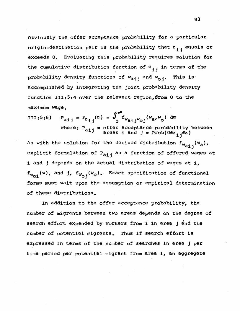
93
Obviously the offer acceptance probability for a particular
origin-destination pair is the probability that z equals or
exceeds 0. Evaluating this probability requires solution for
the cumulative distribution function of Z in terms of the
probability density functions of waij and we . This is-
accomplished by integrating the joint probability density
function 111:5:4 over the relevent regionfrom 0 to the
maximum wage.
111:5:6) Paij = Fz Sf waijwo(wa,wo) d
where: P = offer acceptance probability betweenareas i and j.= Prob(Oz !5z)i j
As with the solution for the derived distribution fwaij(wa)
explicit formulation of Paij as a function of offered wages at
i and j depends on the actual distribution of wages at i,
f (w), and J, fw (wo). Exact specification of functional
forms must wait upon the assumption or empirical determination
of these distributions.
In addition to the offer acceptance probability, the
number of migrants between two areas depends on the degree of
search effort expended by workers from i in area j and the
number of potential migrants. Thus if search effort is
expressed in terms of the number of searches in area j per
time period per potential migrant from area i, an aggregate
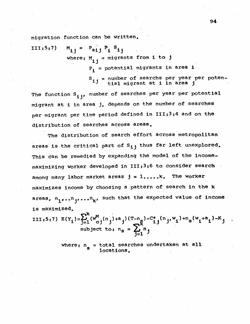
94
migration function can be written.
111:5:7) M = P P Sij aij £ ij
where: M = migrants from i to jij
P = potential migrants in area i
S = number of searchs per year per poten-tial migrant at i in area j
The function Si, number of searches per year per potential
migrant at i in area j, depends on the number of searches
per migrant per time period defined in 111:3:4 and on the
distribution of searches across areas.
The distribution of search effort across metropolitan
areas is the critical part of Sij thus far left unexplored.
This can be remedied by expanding the model of the income-
maximizing worker developed in 111:3:6 to consider search
among many labor market areas j = 1.... .k. The worker
maximizes income by choosing a pattern of search in the. k
areas, nl,..n , k, such that the expected value of income
is maximized,
111:5:7) E(Y)P(WM (n )+a )(T-n )-C* (n w )+ns i+a )-K
subject to: n.= n
where: n = total searches undertaken at alls locations.
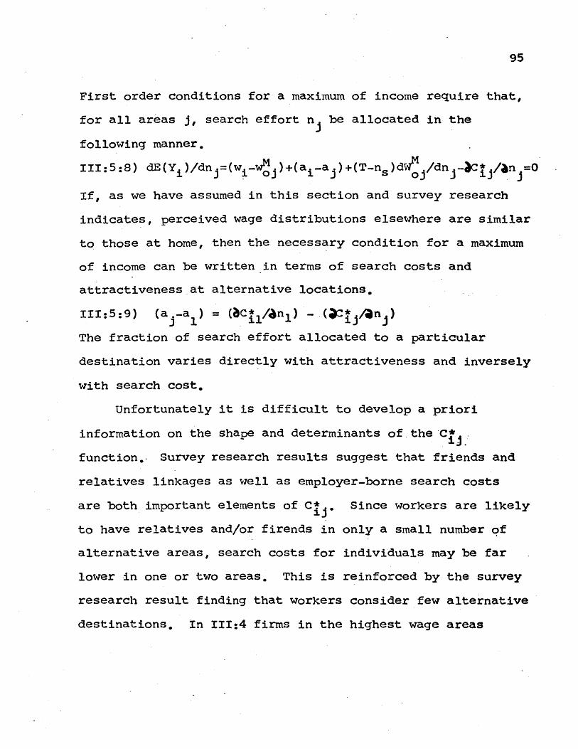
95
First order conditions for a maximum of income require that,
for all areas j, search effort n be allocated in the
following manner.
111:5:8) dE(Y )/dnj=(w - )+(a a )+(T-ns)d /dn -C* /an =0J j i oj j- ii J
If, as we have assumed in this section and survey research
indicates, perceived wage distributions elsewhere are similar
to those at home, then the necessary condition for a maximum
of income can be written in terms of search costs and
attractiveness at alternative locations.
111:5:9) (a -al) = Anl) - /n
The fraction of search effort allocated to a particular
destination varies directly with attractiveness and inversely
with search cost.
Unfortunately it is difficult to develop a priori
information on the shape and determinants of the C*
function.. Survey research results suggest that friends and
relatives linkages as well as employer-borne search costs
are both important elements of C* Since workers are likely
to have relatives and/or firends in only a small number of
alternative areas, search costs for individuals may be far
lower in one or two areas. This is reinforced by the survey
research result finding that workers consider few alternative
destinations. In 111:4 firms in the highest wage areas

96
were shown to realize a return from investing in employee
search in low-wage areas, once again this suggests that
search costs in a few destinations will be lower than others.
In this case high-wage areas would have the lowest costs,
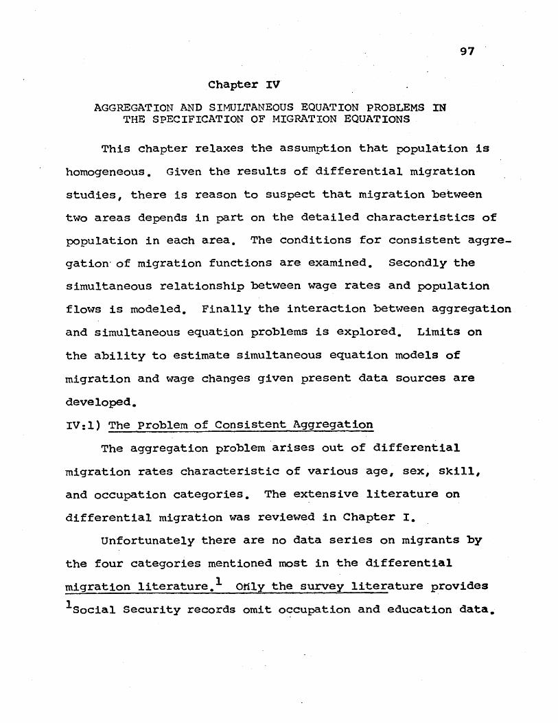
97
Chapter IV
AGGREGATION AND SIMULTANEOUS EQUATION PROBLEMS INTHE SPECIFICATION OF MIGRATION EQUATIONS
This chapter relaxes the assumption that population is
homogeneous. Given the results of differential migration
studies, there is reason to suspect that migration between
two areas depends in part on the detailed characteristics of
population in each area. The conditions for consistent aggre-
gation- of migration functions are examined. Secondly the
simultaneous relationship between wage rates and population
flows is modeled. Finally the interaction between aggregation
and simultaneous equation problems is explored. Limits on
the ability to estimate simultaneous equation models of
migration and wage changes given present data sources are
developed.
IV:1) The Problem of Consistent Aggregation
The aggregation problem arises out of differential
migration rates characteristic of various age, sex, skill,
and occupation categories. The extensive literature on
differential migration was reviewed in Chapter I.
Unfortunately there are no data series on migrants by
the four categories mentioned most in the differential
migration literature.1 Only the survey literature provides
lSocial Security records omit occupation and education data*
98
a source of individual record data by detailed demographic
categories. Thus there is a basic need to deal with
aggregate migration functions.
In the case of migration functions developed above,
acute aggregation problems reside in the offer acceptance
probability function. These will be demonstrated in terms
of a simple model.
Consider the offer-acceptance probability to depend on
two categories of variables, The first variable will be
called a wage and is specific to a single demographic groups
age, sex7 occupation; and education category. The second
variable will be termed an environmental or public good
variable because it represents attributes of an area that
affect all residents of the locality equally. Notable
examples are price indexes, environmental quality, public
goods, climate, etc.
Now the offer acceptance probability for migration
between origin i and destination j will depend on the wage
k kvariables W, and W characteristic of demographic group
k = 1,2,,..m. We have suggested that the wage at each
location will generally be a stochastic variable but for
this discussion may be regarded as deterministic, The
single environmental or public good variable of interest for
areas i and j will be G and G .
99
The individual offer acceptance probabilities for each
of the m demographic groups, , po.., k , mayaiji aij*** aij# a
be expressed in terms of the notation developed above as:
IV:1:1) p =P 1 ( W1 G , W1 G )Pai ai i'*
p aij - aij( Wk 0Gi, Wk 0 G~0 0
p = P ( Wi, G, W Gp P ( , G ,W , G )
The problem of consistent aggregation involves finding
the following three functions:
IV:1:2) Ag( W1 W2 W , = W
IV:1:3) AW ( W , W2 ,... Wk ... W) =WTi j ij ' ''' i j ' ''' i i
IV:l:4) A (i *of k m = TPaij aij' Paij'** Paij) Paij
Where IV:1:2 through IV:1:4 are chosen such that an aggregate
migration function may be written in terms that sacrifice none
of the behavioral results contained in the original functions,
giving:
IV:1:5) pT Aaj WT , G , WT , G)
Aggregate migration functions require that the existence and
functional form of Aw,, A, and APaij be demonstrated on the
basis of a priori information arising from behavorial
assumptions of the migration model. The conditions for con.-
sistent aggregation may require -making strong and restrictive
assumotions about the behavior of migrants.
1The discussion of migration presented here relies on anextensive literature on aggregation problems developed inother contexts,
100
There are strong a priori restrictions on the form of
the A function. Aggregate acceptance probability dependsPa jj
on the acceptance probability of each individual demographic
group weighted according to the fraction of total origin
population in that demographic category.T k k
IV:1:6) pT pC N/N
where: N = total population at the origin
N = the number of type k individuals atthe origin.
This is the form of the APaij function which is implied by
the use of offer acceptance probability within the job-search
model of migration developed in the previous chapter.
Aggregate wage indexes for states and metropolitan areas
generally assume the form:
IV:1:7) W = E N k I/N
IV:1:8) WT = I E k N I/Nj k= j iii
where: E = the fraction of demographic group kactually employed in area i
E = the fraction of demographic group kactually employed in area j.
The E and E terms function as weights indicating the
participation of each demographic group in the activity to
which the wage variables, Wk and Wk, refer. In this case
the activity is measured employment.
101
Now that specific functional forms have been specified
for AW , AW, and A aij, necessary conditions for the exist.
ence of an aggregate migration function based on these
aggregating functions may be derived. Consistent aggregation
requires thatfor any change in the Wk or Wk variables that£ j
leaves AWi and AWj unchanged,in equation IV:1:5, p must
also be unchanged. There are six different categories of
necessary conditions.
IV:1:9) p /W = p / W for all k = 1....m
IV:1:lO) yp i/)W~ = /) for all kc = 1..
IV:1:ll) )pij/?G = Ii/bGi for all kc = l..
IV:1:12) p J/0G = pi/k G for all k =
IV:1:13) E =E for all k = 2....m
E = for all k = 2....m
IV:1:14) N/N = N/N for all k = 1....m
The job-search models developed in the previous chapter
suggest that the functions p ij/Wk, l / -s ,p /aGi,
and /4G are not only not constants but indeed that they
are non'linear in many cases, Obviously furthur conditions
k W G kand G kareconnecting the values taken on by W , W ,
necessary if conditions IV:1:9 through IV:1:12 are to be
satisfied.
Condition IV:1:13 requires that the participation rates,
Ek and Ek be the same for all demographic groups in each
102
area. if the wage variables are considered to refer only to
hourly earnings of employees then this condition requires
equal employment rates for all demographic groups, here the
employment rate, the fraction of the group actually employed,
functions as the participation rate, As long as the groups.
considered consist only of "prime age" males, 25 to 64 years
of age, this assumption may approximate reality. Clearly
the assumption is not valid for the population in general.
Indeed the literature surveyed earlier suggested that even
among"prime age" males the ratio of white to non-white
unemployment rates is not only not equal to one everywhere
but that it also varies systematically across geographic
areas.1
The final condition for consistent aggregation, IV:1:14,
requires that the population composition at both the origin
and destination be identical. This is most unlikely.
Fortunately this condition is the simple product of the
manner in which the aggregate destination wage was computed.
Thus if the same weights are used for AW as for AWi as shown
in IV:1:15 below, the last condition for consistent aggrega.
tion will besatisfied,
IV:1:15) WT = E1 N /N
Similarly the most obvious mechanism for dealing with
differences in participation rates among demographic groups1 See, for example: Rapping,L.A.,Unionism, Migration and the &Male Nonwhite-White Unemployment DifferentialSouthernEconomic Journal, Vol, 32,No, 3, (July, 1966),pp. 317-329,
103
is to compute the A and AWj based on the assumption that
the participation rates Ek and Ek are uniformly equal toij
one.
Given these modifications in A and Aw designed to
deal with conditions IV:1:13 and IV:1:14, strong questions
concerning whether conditions IV:1:9 through IV:1:12 remain.
To the extent that these questions involve empirical issues
they will be discussed in subsequent sections.
IV:2) Determinants Of Differential Migration
The extensive literature on differential migration
suggests that rates of migration vary by age, sex, race,
occupation, and education. Such results cannot be taken as
positive evidence that the partial response of different
demographic groups to given incentives for migration varies
systematically. Indeed these studies do not consider the
possibility that differential migration may be due to
differences in the incentive to migration for each group.
Thus the demand side of the labor iarket is virtually
ignored.
This section will attempt to determine the fraction of
total migration differentials which is related to differences
in mobility among demographic groups, adjusted for demand
side effects. The basic rationale for the existence of
pure differences in the migratory response of different
104
groups to equal incentives is based on delective attraction
of a fixed residence, Age, and education would seem to be
particularly related to the apparent sluggishness or ease
with which groups respond to given opportunities for migra-
tion. Specifically it might be expected that older and less
well educated individuals would be reluctant to change
residence.
In the tables below the relative propensities of various
demographic groups to migrate between metropolitan areas is
compared with the relative fractions of the same groups to
change their place of residence within the area. This second
figure should reflect the attitude of the various groups
toward changes in residence in general. As might be expected,
there are systematic differences in the fraction of various
groups which change residence within metropolitan areas that
parallel observed behavior of migrants. However only a
fraction of differential migration rates is related to the
differences within areas. Residual differences in )the
propensity to migrate that remain can be attributed to a
muddled combination of "pure" differences in incentives to
migrate including the preferences of employers and the
availability of information on opportunities elsewhere.
Table IV:2:1 below presents the relationship between
intra-metropolitan and inter-metropolitan mobility rates for
Also monetary and psycic costs of moving may vary byfamily type and family size in particular.
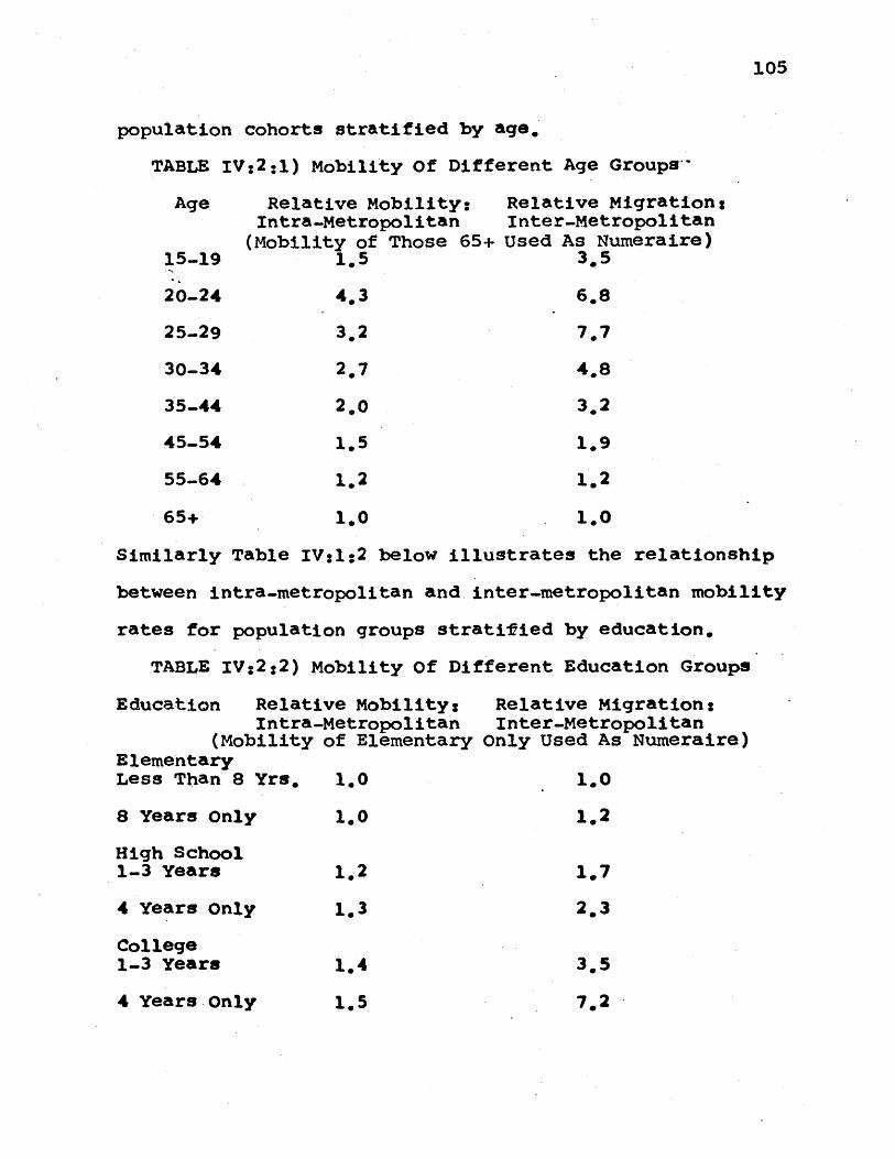
105
population cohorts stratified by age.
TABLE IV:2:1) Mobility Of Different Age Groups'
Age Relative Mobility: Relative Migration:Intra-Metropolitan Inter-Metropolitan
(Mobility of Those 65+ Used As Numeraire)15-19 1,5 3.5
20-24 4,3 6,8
25-29 3.2 7,7
30-34 2,7 4,8
35-44 2.0 3.2
45-54 1.5 1.9
55-64 1,2 1,2
65+ 1,0 1,0
Similarly Table IV:1:2 below illustrates the relationship
between intra-metropolitan and inter-metropolitan mobility
rates for population groups stratified by education.
TABLE IV:2:2) Mobility Of Different Education Groups
Education Relative Mobility: Relative Migration:Intra-Metropolitan Inter-Metropolitan
(Mobility of Elementary Only Used As Numeraire)ElementaryLess Than 8 Yrs, 1.0 1.0
8 Years only 1,0 1,2
High School1.3 Years 1,2 1.7
4 Years only 1,3 2*3
College1-3 Years 1,4 3.5
4 Years only 1.5 7.2
106
The source of data for both tables above is the 1960 Census of
Population. Age and education are the two principal a priori
sources of differences in the willingness of individuals to
move, For both the age and education variables the indicated
intra and inter-metropolitan mobility patterns are closely
related. For "prime age" males the rank order of mobility
rates is identical within and between areas. This simple test
indicates that perhaps half of observed differential migration
rates for age cohorts may arise from differences in the "pure"
reluctance to change residential location. For education
cohorts, increasing educational attainment is related positive-
ly to increasing mobility both within and between areas, Much
of the difference in mobility by age and education is due to
preferences of employers and job rights accrued by older,
blue-collar workers. But these factors should affect both
differential mobility within and between cities. However,
intra-metropolitan mobility differentials account for only a
small fraction of the very high differential migration rates
based on age and education. Thus the propensity to migrate in
the face of given opportunities is related to age and educa-
tion. Unfortunately data on characteristics of migrants
1 Data are based on a sample of movers within the populationof 15 SMSA's chosen randomly from: US. Bureau of the Census,Mobility For States And Metropolitan Areas, PC(2)-2B,Washington, D.C.: US, Government Printing Office, (1963)
107
between metropolitan areas and within them by both age and
education characteristics was not found.
The inquiry in this section was motivated by the necess.
ary conditions for consistent aggregation, particularly the
first four conditions which required that p /Wk, p /
gP ij/aGi, and qpik /CG be equal for all demographic groups
k. The results suggest that,particularly for groups represen-
ting different age cohorts, such assumptions of equal marginal
response to changes in wages or general attractiveness at the
origin or destination are not supported by empirical evidence.
IV:3) A Simple Model of The Simultaneous Equation Problem
Migration equations are part of the fundamental growth
equations for a metropolitan area. Some of the variables
proposed above as arguments of the migration equations are
also endogeneous to comprehensive models of metropolitan
development. This is particularly true of wages. There is
a danger of simultaneous equation bias in attempting to
estimate the parameters of a migration equation .when current
values of endogeneous variables are included in the equation.
This section developes a simple aggregate model of
metropolitan development that illustrates the nature of
simultaneous equation bias that might accompany use of wage
variables in a migration equation. Recently there have been
lobviously a more comprehensive data base is needed to quanti-fy these partial derivitives exactly.
108
some efforts to develop simultaneous equation models of
migration and metropolitan growth. None of these efforts
has resulted in a full structural model and one even holds
wages to be a fundamental exogeneous variable.
Consider the following static equilibrium model of a
metropolitan area. Total output per time period is deter-
mined by an aggregate production function involving homogen-
eous capital and labor.
IV:3:1) Q = F(KL)
where: Q = total output of homogeneous goods
K = units of homogeneous capital
L = units of homogeneous labor
aQ/JK and )Q/JL are both positive
Q/K2 and YQ/)L2 are both negative
Demand for the output of the area depends on the price of
output and on the total wage bill of the area. This second
determinant of demand is due to the high transportation costs
associated with many goods and is analogous to similar assump.
tions made in economic base models.
IV:3:2) S = D(P, WL)
where: S = total sales of.homogeneous output
See, for example: Olvey, Lee Donne, "Regional Growth AndInterregional Migration," Unpublished Harvard Ph.D.Dissertation, (April, 1970) and Muth, Richard, "DifferentialGrowth Among Large U.S. Cities," in James P, Quirk and ArvidM. Zarley, eds., Papers in Quantitative Economics, (Lawrence,Kansas: The University Press of Kansas), 1968, pp.3 11- 3 5 5.
109
where: P = price of output of the area
W = money wages in the area
;S/)p is negatiVen
*S/OWL is positive
The product market is closed by equating sales and output
so that there is no net change in inventories.
IV:3:3) S = Q
In specifying the area demand function, the price of goods
produced elsewhere is set equal to unity.
Factor markets in the metropolitan area,are assumed to
be perfectly competitive and supply curves for capital and
labor are assumed sufficiently price elastic to achieve a
market clearing equilibrium with no unemployment or excess
capacity. There is no non-price rationing in factor markets.
The supply of capital depends on relative rates of return in
the area and the rest of the world, or nation, or region.
IV:3:4) K,= k( R/r )
where: R = rate of return on capital in the area
r = rate of return on capital elsewhere
dk/d(R/r) is positive
The supply of labor includes the migration function. Here
migration is assumed to depend only on the ratio of real
wages available in the area to the real wage rates prevailing
1These strong assumptions concerning the nature of the marketclearing solution are not strictly necessary. The presenceof excess capacity or unemployment could be incorporated inthe rate of return and wage variables respectively.
110
elsewhere.
IV:3:5) L = M( W/P, w ) = M( W/Pw )
where: W = money wages in the area
P = price of output of the area
W = money wages available elsewhere
dL/d(W/Pw) is positive
Note that since the price level elsewhere is unity, w is
also the real wage elsewhere. Finally the factor markets
are closed, given the assumptions of no unemployment or ex.-
cess capacity, by equating the rate of return on capital and
the mbney wage to the value of the marginal physical product
of capital and labor respectively.
IV:3:6) W = P ()F/4L )
IV:3:7) R = P (IF/AK )
The model now consists of seven equations in seven
endogeneous variables, Q, S, K, L, W, R, and P, and three
exogeneous variables including w, r, and prices elsewhere
which were set equal to unity. Included in structural equa-
tion IV:3:5 is a standard migration function. The-simultan-
eous equation problem involves determination of the conseq-
uences of attempting to estimate migration between the
metropolitan area and other, areas using a single equation
It might be objected that real wages in the metropolitanarea should be based on a weighted index of prices withinand outside the area. The example here can be taken as theextreme case of weights equal to 1 and 0 respectively.
111
model.
Such a single equation approach would involve attempting
to estimate equation IV:3:5 directly. If W, P, w, and prices
elsewhere were all exogeneous, such an equation could be
estimated and the partial relatenships between changes in
each of these variables and net migration flows determined.
However, real wages in the metropolitan area, W/P, appear in
IV:3:6 as a function of aF/JL, which will in general have L,
total labor force in the area, as one of its arguments. In-
deed we have implicitly assumed this to be the case by
assuming )F/t)L to be positive and wF/3L2 to be negative.
Thus equations IV:3:5 and IV:3:6 combine to yield a classic
case of simple simultaneous equation bias if estimated in
a single equation model.
IV:3:5) L = M( W/P, w )
IV:3:6) W/P = 3F/)L
Attempts to estimate a simple linear version of IV:3:5 and
IV:3:6 illustrate the bias in a concrete context. Rewriting
these two equations in terms of observed wages and migration
gives:
IV:3:8) L =a 0 + a (W/p) + a2w + u
IV:3:9) W/P = b0 + bjL + e
This ignores aggregation problems discussed earlier
112
where: u and e = distrubances reflecting effectsof other variables.
Single equation models attempt to estimate IV:3:8 directly
and interpret the parameter a, as the partial derivitive of
migration with respect to changes in real wages, )L/a(W/p).
But these variables are connected by a second expression,
IV:3:9. If, as a priori conditions suggest, b1 is negative,
then the covariance of u and (W/P) will be negative. Attempts
to estimate IV:3:8 by ordinary least squares will result in
a downward bias in estimates of a due to the negative
covariance between W/P and the residual term u.
Difficulties inherint in single equation estimates drawn
from the structural model have led researchers to estimate
reduced form relationships between wages and population change.
This reduced form approach has been the subject of extensive
empirical work reviewed in Chapter 11:3. The seven equation
system, IV:3:1 through IV:3:7, can be evaluated using compara-
tive statics for the total derivitive of population with
respect to changes in exogeneous external wages.
IV:3:lO) dL -M/W - (M/aW)dW~ (aF/c)L - bD/bL)(aM/5W)/(6D/6W)
If worker wages are larger than expenditures on local goods,
( F/ L - D/ L) is positive. Since ( M/ W) and ( D/ W) are
both positive, the two terms on the right side of IV:3:10
have opposite signs. Thus the sigh of dL/dw is ambiguous.
This result agrees with empirical evidence.
113
The arguments presented above leave the impression that
the simultaneous equation problem only concerns the coeffic-.
ient of W/P in the migration equation. But there are furthur
problems involved in estimating the migration equation
presented in this simultaneous equation model. Careful
examination shows that the migration equation is not
identified. The only excluded exogeneous variable is r and
there are at least two included endogeneous variables. This
is not intended to suggest that it is not possible to formu-
late simultaneous equation models in which there is sufficient
a priori information to identify the migration equation, but
the data and theory requirements of such models might be
extensive.
IV:4) Interaction Between Aggregation And Simultaneous
Equation Problems
The greatest difficulty in implementing simultaneous
eqation models results from the interaction of aggregation
and simultaneous equation problems. The simple model
presented above involved homogeneous labor and capital.
Of course labor is heterogeneous and, most important, there
is a systematic relationship between relative mobility of
different groups and the wages of these groups. This
systematic relationship tends to obscure the size and
114
direction of the change in money wages accompanying a change
in labor force due to net migration flows.
The aggregation problem arises in equation IV:3:6 of
the model presented in the previous section because actual
wage data is only available in dollars per manhour by
industry or, less readily, by occupation for metropolitan
areas. There is little if any possibility of constructing
a wage index based on the level of compensation for given
education, or skill.I But migration-rates tend to increase
very sharply with the number of years of education. It is
well known that areas of chronic heavy net out migration
accumulate unskilled and uneducated workers in exceptional
concentrations. The strong relationship between education
and relative mobility is presented in Table IV:2:2 above.
Thus areas experiencing large inflows of migrants will
tend to find the average educational level of their work force
increasing. This will tend, ceteris parAbus, to cause the
wage index, based on compensation per manhour, to rise for
such areas. This effect is directly opposed to direction of
wage determination in the productivity equation which suggests
increases in the labor force are associated, ceteris parabus,
with a decline in wages.
These effects may be analyzed in terms of a simple model.
The greatest empirical difficulty involved in constructingsuch an index is that the level of educational achievementrepresented by given years spent in school varies by region.
115
In the model presented in the previous section# real wages
per manhour of homogeneous labor were determined in a simple
productivity equation.
IV:4:l) W = aQ/aL
where: W = real wages per manhour
Q = output
L = manhours of homogeneous labor
The real wage index used here is based on the format in which
the;dattaaate normally computed and used in migration models.
The total wage bill is deflated by a price index and divided
by total manhours. There is an unambiguous relationship
between migration flows that change the size of the labor
force by adding more units of homogeneous labor and resulting
wage dhanges.
IVt4:2) bW/L = co/&L2
This formulation implicitly assumes that migrants are not
distinguishable from the population in general.
If workers are differentiated by skill or education level,
the production function must be reformulated to indicate the
effect of these skills on total output from given capital
and manhours. One way of formalizing the effect of skill
levels on output is to measure labor input in equivalent
efficiency units of labor.
116
IV:4:3) Q = F( K, H )
where: H = total labor input in efficiency units
Similarly wages per efficiency unit of labor may be defined.
IV:4:4) E = H
where: E = real wages per efficiency unit of labor
The real wage per manhour in the area is equal to the
real wage per efficiency unit of labor multiplied by average
level of efficiency units per worker.
IV:4:5) W = E (H/L )
Now if the area recetves immigrants from another region the
effect on measured real wages per manhour may be found by
evaluating the total differential of IV:4:5.
IV:4:6) dW/dL = ( )W/E )dE/dL + ( clW/H )dH/dL + ( gW/3L )
This may be rewritten after appropriate substitution as:
IV:4:7) dW/dL = (H/L)dE/dL + (E/L)dH/dL - EH/L2
If the level of efficiency units per immigrant is known, the
impact of migration on measured real wages may be furthur
evaluated.
IV:4:8) dE/dL = (dB/dH)(dH/dL) = ( 2Q/H ) h
IV:4:9) dH/dL = h
where: h = efficiency units per migrant.
Substituting the results of IV:4:8 and IV:4:9 into IV:4:7
gives a much more satisfying expression for the change in
the real wage per manhour.
117
IV:4:1O) dW/dL = (H/L)(a0/ZH2 )h + (E/L)h - (E/L)(H/L)
Noting that (H/L) is the efficiency units per worker in the
area, we can rewrite IV:4:l0 so that the sign of dW/dL can
be expressed in terms of the difference in skill level bet-
ween migrants and resident workers,
IV:4:ll) dW/dL = (H/L)h(Q/aH 2 ) + (E/L) ( h H/L )
where: (H/L)h(IQ/AH2 ) 4 0
Thus the sign of dW/dL depends on the relationship between
h and H/L,
There is strong evidence that h is larger than H/L.
Migrants ace lfar mOreeducated than the general population,
Thus even if the capital stock and technology are unchanged
the total effect of immigration on the real wage per manhour
is ambiguous. Indeed, to the extent that migrants are far
more skilled than the general workforce, real wages per man-.
hour may rise in areas receiving large migrant inflows!
Conversely real wages per manhour may fall in areas losing
population through migration,
118
CHAPTER V
EMPIRICAL TESTS OF THE MODEL
This chapter contains an empirical evaluation of the
job-search model of migration developed in Chapter III mindful
always of the difficulties catalogued in Chapter IV. Data
limitations are a constant hindrance to empirical work on
migration and the model specifications presented here
represent an attempt to adapt theory to available data. The
nest two sections of this chapter develop a particular
specification of an aggregate migration function and possible
strategies for promoting consistent aggregation. Finally
estimates of migration functions are made using data on
migration from the United States and United Kingdom.
V:l) Specification Of An Aggregate Migration Function
In chapter III the necessity of making assumptions
concerning the actual distributions of wages in different
areas was pointed out. Inevitably there is an element of
arbitrary specification in choice of wage distributions since,
due largely to lack of data, there is little literature on
this topic. Given the limited availability of data on
migration and wages, it is not clear that an elegant formula-
tion of wage distributions would make it possible to estimate
more precise functions.
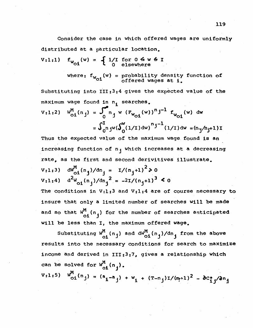
119
Consider the case in which offered wages are uniformly
distributed at a particular location.
V:1:1) f (w) = 1/I for 0 4 w 6 Iwoi 0 elsewhere
where: f (w) = probability density function ofwoi offered wages at i.
Substituting into 111:3:4 gives the expected value of the
maximum wage found in n searches.
V:1:2) W' (nj) = Jrn w (FW (w))nj-1 (w) dw
1 WIn -1= 0 n jw(S (1/I)dw)i (1/I)dw =(n /ng+1)I
Thus the expected value of the maximum wage found is an
increasing function of nj which increases at a decreasing
rate, as the first and second derivitives illustrate.
V:1:3) dW (n )/dn= I/(n +1) > 0
V:1:4) d2W (n )/dn 2= .2I/(n +1) 3 < 0
The conditions in V:1:3 and V:1:4 are of course necessary to
insure that only a limited number of searches will be made
and so that W (n ) for the number of searches anticipatedoij
will be less than I, the maximum offered wage.
Substituting WM (nj) and dWM (n )/dn from the above
results into the necessary conditions for search to maximize
income and derived in 111:3:7, gives a relationship which
can be solved for WM (n ).oi j
Vo:5 inJ) = (a i-a) + w~ + (T-nj)I/ii4+l) /)
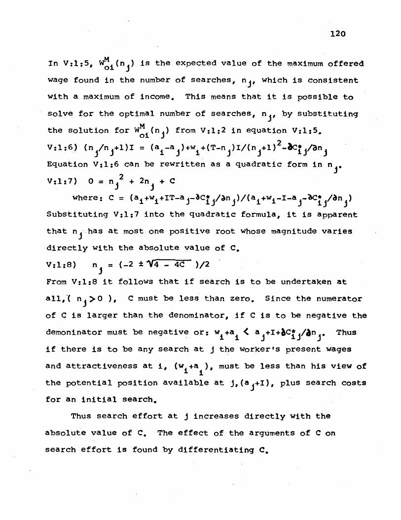
120
In V:1:5, WM (n is the expected value of the maximum offered
wage found in the number of searches, n , which is consistent
with a maximum of income. This means that it is possible to
solve for the optimal number of searches, n,, by substituting
the solution for W (nj) from V:1:2 in equation V:1:5.
V:1:6) (n /n +1)I = (a -a )+w +(T-n )I/(n +1)2
Equation V:1:6 can be rewritten as a quadratic form in n .
V:1:7) 0 = n 2 + 2n + C
where: C = (a +w +IT-a -C*/An )/(a +w -I-a -C* /8n )
Substituting V:1:7 into the quadratic formula, it is apparent
that n has at most one positive root whose magnitude varies
directly with the absolute value of C.
V:1:8) n = (-2 * %4 - 4C )/2
From V:1:8 it follows that if search is to be undertaken at
all,'( n >0 ), C must be less than zero. Since the numerator
of C is larger than the denominator, if C is to be negative the
demoninator must be negative or: w +a. < a +I+bC*/an . Thus
if there is to be any search at j the worker's present wages
and attractiveness at i, (w +a ), must be less than his view of
the potential position available at j,(a +I), plus search costs
for an initial search.
Thus search effort at j increases directly with the
absolute value of C. The effect of the arguments of C on
search effort is found by differentiating C.
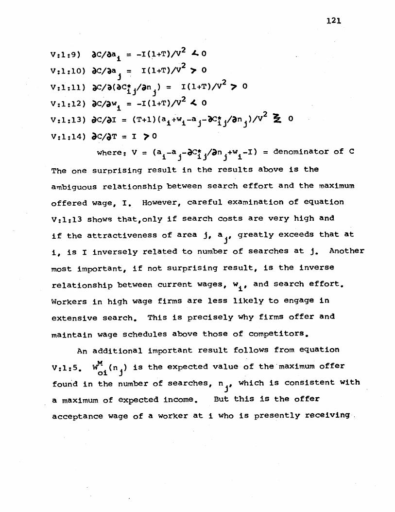
121
V:1:9) 3C/aa = -I(1+T)/V 2 4. 0
2V:1:10) aC/aa = I(1+T)/V 7P 0
V:1:1l) aC/a(aC /n) = I(l+T)/V 2 -0 0
V:1:12) 3C/aw = -I(1+T)/V 2 4 0
V:1:13) )C/aI = (T+1)(aj+w -a -IC* /an )/V 2 i 0
V:1:14) aC/4T = I 7 0
where: V = (a.-a .- gC ,/an .+w.-I) = denominator of C. J - 1J' - ) I.
The one surprising result in the results above is the
ambiguous relationship between search effort and the maximum
offered wage, I. However, careful examination of equation
V:1:13 shows thatonly if search costs are very high and
if the attractiveness of area j, a , greatly exceeds that at
i, is I inversely related to number of searches at J. Another
most important, if not surprising result, is the inverse
relationship between current wages, wi, and search effort.
Workers in high wage firms are less likely to engage in
extensive search. This is precisely why firms offer and
maintain wage schedules above those of competitors.
An additional important result follows from equation
V:1:5. WM (n ) is the expected value of the maximum offeroi j
found in the number of searches, n , which is consistent with
a maximum of expected income. But this is the offer
acceptance wage of a worker at i who is presently receiving,.
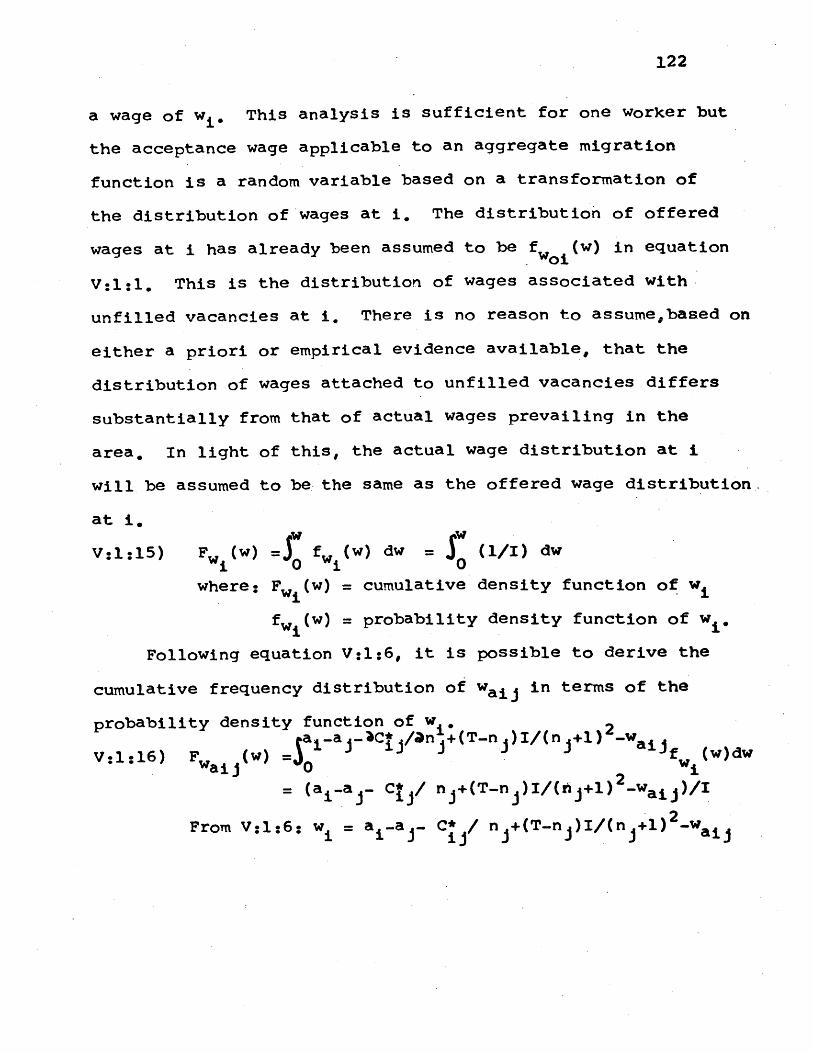
122
a wage of w1 , This analysis is sufficient for one worker but
the acceptance wage applicable to an aggregate migration
function is a random variable based on a transformation of
the distribution of wages at i. The distribution of offered
wages at i has already been assumed to be f (w) in equationwol
V:1:1. This is the distribution of wages associated with
unfilled vacancIes at I There is no reason to assume*based on
either a priori or empirical evidence available, that the
distribution of wages attached to unfilled vacancies differs
substantially from that of actual wages prevailing in the
area. In light of this, the actual wage distribution at i
will be assumed to be the same as the offered wage distribution
at I.
V:1:15) F (w) = f (w) dw = (1/I) dw
where: Fwi(w) = cumulative density function of w
fwj(w) = probability density function of w I
Following equation V:1:6, it is possible to derive the
cumulative frequency distribution of waij in terms of the
probability density function of w 2
- a-C*/,n +(T-n )I/(n +1) -waV:1:16) F (w) = if (w)dw
wa_ 0= (a -aj- C / n +(T-n )I/(ri+l)2 -wao V 1 w = a awaij)
From V:1:6: w a C* /n 2(-jI(n+ wi
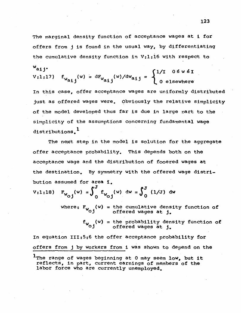
123
The marginal density function of acceptance wages at i for
offers from j is found in the usual way, by differentiating
the cumulative density function in V:1:16 with respect to
Waij* 1/I O!! w 4I
V:1:17) f (w) = dFw (w)/dwaij = elsewhere
In this case, offer acceptance wages are uniformly distributed
just as offered wages were. Obviously the relative simplicity
of the model developed thus far is due in large part to the
simplicity of the assumptions concerning fundamental wage
distributions.
The next step in the model is solution for the aggregate
offer acceptance probability. This depends both on the
acceptance wage and the distribution of fooered wages at
the destination. By symmetry with the offered wage distri-
bution assumed for area i,
V:1:18) F wj(w) = f (w) dw =J (1/J) dw
where: F (w) = the cumulative density function ofwoj offered wages at j,
f (w) = the probability density function ofwoj offered wages at J.
In equation 111:5:6 the offer acceptance probability for
offers from j by workers from i was shown to depend on the
1The range of wages beginning at 0 may seem low, but itreflects, in part, current earnings of members of thelabor force who are currently unemployed.
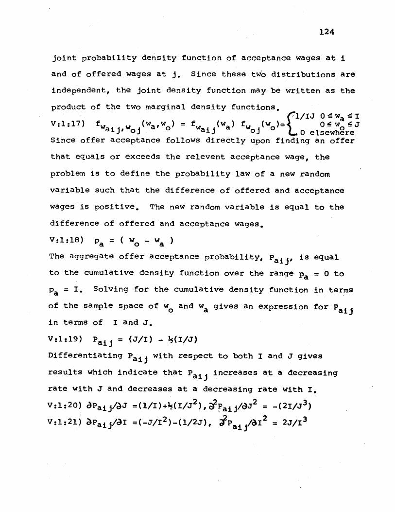
124
joint probability density function of acceptance wages at i
and of offered wages at j. Since these two distributions are
independent, the joint density function may be written as the
product of the two marginal density functions,1/IJ 0 If wa 1
V:1:17) f waiJ#'wOJ(wa,wo) = fwaij (w a) f wJ (w)= 0 w Ja 0 elsewhere
Since offer acceptance follows directly upon finding an offer
that equals or exceeds the relevent acceptance wage, the
problem is to define the probability law of a new random
variable such that the difference of offered and acceptance
wages is positive. The new random variable is equal to the
difference of offered and acceptance wages.
V:1:18) pa = ( wo - wa
The aggregate offer acceptance probability, P , is equal
to the cumulative density function over the range pa = 0 to
pa = I. Solving for the cumulative density function in terms
of the sample space of w0 and wa gives an expression for Paij
in terms of I and J.
V:1:19) Pa (J/I) - (I/J)
Differentiating Pat with respect to both I and J gives
results which indicate that P increases at a decreasingaij
rate with J and decreases at a decreasing rate with I.
V:1:20) cPaij/ J =(l/I)+ (I/J 2 ), Paij/dJ2 = -(2I/J3
V:1:21) *Paij/ I =(_J/1 2 )-(1/2J), P aiAI2 = 2J/1 3
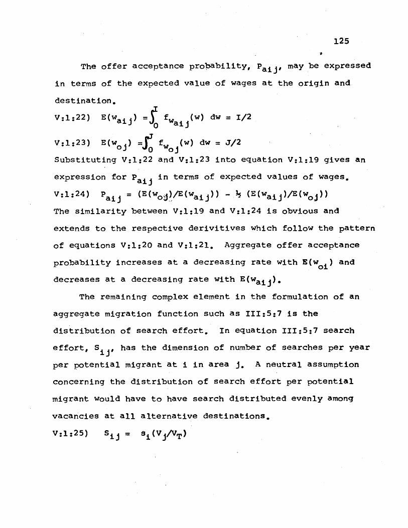
125
The offer acceptance probability, Paij, may be expressed
in terms of the expected value of wages at the origin and
destination,
V:1:22) E(waij) fw aij(w) dw = I/2
V:1:23) E(w ) J fwo (w) dw = J/2oj oj
Substituting V:1:22 and V:1:23 into equation V:1:19 gives an
expression for P aj in terms of expected values of wages,
V:1:24) Paij = (E(woj)/E(waij)) - (E(waij)/E(woj))
The similarity between V:1:19 and V:1:24 is obvious and
extends to the respective derivitives which follow the pattern
of equations V:1:20 and V:1:21. Aggregate offer acceptance
probability increases at a decreasing rate with E(w ) and
decreases at a decreasing rate with E(waij)-
The remaining complex element in the formulation of an
aggregate migration function such as 111:5:7 is the
distribution of search effort, In equation 111:5:7 search
effort, S , has the dimension of number of searches per year
per potential migrant at i in area j. A neutral assumption
concerning the distribution of search effort per potential
migrant would have to have search distributed evenly among
vacancies at all alternative destinations,
V:1:25) Sij = Si(V J/VT)
126
where: V = job vacancies in area j
VT = total vacancies at all locations
s = constant of proportionality reflectingthe number of searches per worker pertime period,
Equation V:l:25 obviously involves strong assumptions concern-
ing total search effort and its distributions.
The analysis developed in this section, and particularly
equations V:1:9 through V:1:14, indicates the determinants of
s for a worker at i with wage wi. In general total search
effort at i was found to vary directly with. attractiveness of
the destination, aj; expected duration of employment in the
new job, T7 difference between present wages and maximum wages
at i, (I-wi),. and inversely with attractiveness of the origin,
a , These effects are fairly straightforward in the aggregate
expression developed for search effort, but the difference
between present and maximum wages, (I-wi), varies for each
worker, For all workers at i, the expected value of the
difference (I-w ) is equal to 1/2,. In general the expected
value of the difference between the maximum wage and any
observed wage will increase with the variance of the wage
distribution at i. Thus on the basis of the a priori informa-
tion in equations V:1:9 through V:1:14, the following
127
properties may be attributed to the functional form of si,
V:1:26) si = Si ( T, (a -ai), var(wi) )
where: var(w i) = variance of wages at i.
,S/AjT > 0 from V:1:14
as/a(a -a i)> 0 from V:l:9 and V:l:lo
aS /avar(w )0 from V:1:12 and V:1:14
Thus aggregate search effort at i depends on the time horizon
of workers, the relative attractiveness of i, and the variance
of wages in area i.
The distribution of search effort among alternative
destinations is more complex than the proportional distribution
implied by V:1:25 suggests. Equation 111:5:9 demonstrates that
the sum of attractiveness plus marginal search cost be equal
for all areas searched, Equation V:1:25 may be rewritten to
reflect the influence of attractiveness and search costs on
the distribution of search effort.
V:1:27) S = s (V /VT) d
where: d = differential search effort
The shape of the search cost function is vital to the
determination of the distribution of search effort, d i. If
search costs at one location were lower than at alternative
locations and there were no significant differences in
There is no loss in generality when the s function is writ-ten in terms of the difference in attractiveness, (a -ai),because in V:1:9 and V:1:10 aC/ba and bC/ba have iqualmagnitude and opposite signs,
128
attractiveness, all search effort would be concentrated in one
area.
The search cost function is generally thought to vary
with the distance between origin and destination as well as
the migrant stock from the destination presently in residence
at the origin. The reason for the importance of distance is
that personal trips and interviews are often part of the
search process and are sometimes paid for by workers. Migrant
stock from the destination in residence at the origin is
thought to reduce search costs for individuals who rely on
friends and relatives for labor market information.
In Chapter 111:4 an additional important argument of the
search cost function was developed based on recruiting efforts
of firms at distant locations. Firms were shown to maximize
profits by minimizing recruiting costs. Those firms located
in the highest wage areas were shown in equation 111:4:6 to
recruit more intensively at alternative destinations than firms
in lower wage areas,
Differential search effort defined in equation V:1:27
can be expressed as a function of attractiveness and search
costs.
V:1:28) d = Di ( (a ai), (CiCi ) )
where: (C -C 4 ) = the difference in search costs atthe origin and destination
1 For an elaboration of the migrant stock hypothesis, see:Fabricant, Ruth, "An Expectational Model of Migration," Journalof Regional Science, Vol. 10,(April, 1970), pp. 13-24.
129
Equation 111:4:6 suggests that 3D /ba = -D /ba and theijiiarguments of D are written accordingly as a difference in
attractiveness. Substituting the arguments of C developed
above into V:1:28 gives a new expression for dii
V:1:29) dii = Dii( (a -a ),(C - C 1 (r , M , E(w )) )
where: r = distance between i and j or sometimestransportation cost from i to j is used.
M j= migrant stock from j in residence at i( the summation of past migration flowsfrom j to i
E(w ) = expected value of offered wages at J.oj
This discussion of determinants of the distribution of
search effort among destinations is necessarily less concrete
than other elements of the migration function. The ambiguity
in Dii is due largely to the lack of information, other than
that provided by survey literature, on the search cost
function. There is enough a priori information from the model
in Chapter III to specify the partial effects of the arguments
of Di.
V:1:30) D/ ) 0
V:1:31) )D ii/6C 1 0
V:1:32) cpD ij/,ri j 0
V:1:33) aD /0) > 0
The general assumption in the literature is that migrants fromj to i lower search costs at j for workers in i. There is apossibility that the migrant stock from i at j may lower thecost of searching at j for workers from i. Trivial modifica-tion of the D function would accomodate this assumption.
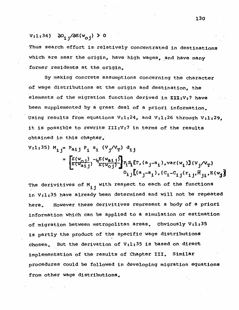
130
V: 1:34) ; D i/aE (w ) > 0
Thus search effort is, relatively concentrated in destinations
which are near the origin, have high wages, and have many
former residents at the origin.
By making concrete assumptions concerning the character
of wage distributions at the origin and destination, the
elements of the migration function derived in KII:V:7 have
been supplemented by a great deal of a priori information.
Using results from equations V:1:24, and V:1:26 through V:1:29,
it is possible to rewrite III:V:7 in terms of the results
obtained in this chapter.
V:1:35) Mii= Paij Pi si (V /VT) dii
11(w E~a)j P EiT, (aj-ai),var (w ).)(V/T
D (a ..a 1)w(Ci-C (rME(w
The derivitives of M with respect to each of the functions
in V:1:35 have already been determined and will not be repeated
here, However these derivitives represent a body of a priori
information which can be applied to a simulation or estimation
of migration between metropolitan areas. obviously V:1:35
is partly the product of the specific wage distributions
chosen. But the derivation of V:1:35 is based on direct
implementation of the results of Chapter III. Similar
procedures could be followed in developing migration equations
from other wage distributions.
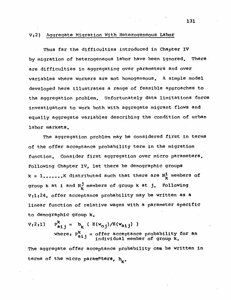
131
V:2) Aggregate Migration With Heterogeneous Labor
Thus far the difficulties introduced in Chapter IV
by migration of heterogeneous labor have been ignored. There
are difficulties in aggregating over parameters and over
variables where workers are not homogeneous. A simple model
developed here illustrates a range of feasible approaches to
the aggregation problem. Unfortunately data limitations force
investigators to work both with aggregate migrant flows and
equally aggregate variables describing the condition of urban
labor markets.
The aggregation problem may be considered first in terms
of the offer acceptance probability term in the migration
function. Consider first aggregation over micro parameters,
Following Chapter IV, let there be demographic groups
k = l.......K distributed such that there are Ni members ofk
group k at i and NJ members of group k at j. Followingk
V:1:24, offer acceptance probability may be written as a
linear function of relative wages with a parameter specific
to demographic group k.
V:2:1) P = bk ( E(woj)/E(waij) -
where: Pk = offer acceptance probability for anaij individual member of group k.
The aggregate offer acceptance probability cam be written in
terms of the micro parameters, bk'
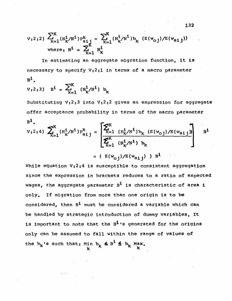
132
V:2:2) K(N/Ni)Pk = (N/N )bk (E(woj)/E(waij))k~l k ai kl
where: N = 2 Nk=1 kc
In estimating an aggregate migration function, it is
necessary to specify V:2:1 in terms of a macro parameter
B.e
V:2:3) B1 = (N1/N1 ) b
Substituting V:2:3 into V:2:2 gives an expression for aggregate
offer acceptance probability in terms of the macro parameter
Bi
V:2:4) (Ni/Ni)P k1 (N/N )bk Bi=1k aij k k(E(woj)/E(waii)i
K-1 (N/N 1 ) b
= ( E(woj)/E(waij) ) B
While equation V:2:4 is susceptible to consistent aggregation
since the expression in brackets reduces to a ratio of expected
wages, the aggregate parameter Bi is characteristic of area i
only. If migration from more than one origin is to be
considered, then Bi must be considered a variable which can
be handled by strategic introduction of dummy variables. It
is important to note that the Bi's generated for the origins
only can be assumed to fall within the range of values of
the bk's such that: Min bk B bk Max.kc kcIc
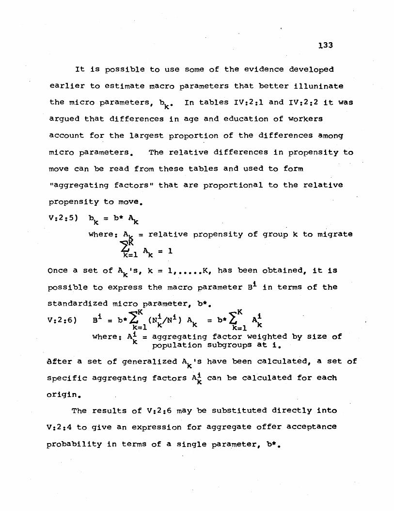
133
It is possible to use some of the evidence developed
earlier to estimate macro parameters that better illuninate
the micro parameters, b In tables IV:2:1 and IV:2:2 it was
argued that differences in age and education of workers
account for the largest proportion of the differences among
micro parameters. The relative differences in propensity to
move can be read from these tables and used to form
"aggregating factors" that are proportional to the relative
propensity to move.
V:2:5) bk = b* Ak
where:A = relative propensity of group k to migrate
k=1 Akk=l k
Once a set of Ak's, k = 1,.....K, has been obtained, it is
possible to express the macro parameter B in terms of the
standardized micro parameter, b*.
V:2:6) Bi = b* (N ) A = b*K AB ~ N*Z k/J k Z~ kk=1 kk=1where: Ai = aggregating factor weighted by size of
k population subgroups at i.
after a set of generalized A k's have been calculated, a set of
specific aggregating factors Ai can be calculated for each
origin.
The results of V:2:6 may be substituted directly into
V:2:4 to give an expression for aggregate offer acceptance
probability in terms of a single parameter, b*,
134
V:2:7) K(N /IN) Pk = b* A (E(W )/E(waij))
In effect the aggregation problem has been incorporated in
the variable Ai, The parameter b* is a constant that may
be estimated consistently in an aggregate crossection study
of migrants from many origins, A set of these aggregating
factors is used in the estimation of aggregate migration
equations in Table V:4:2.
The aggregation problem may also extend to the variables
of a function, specifically the wage variables, Workers are
only qualified for a small fraction of all vacancies. If each
of the K demographic groups has a separate set of jobs, and
hence wages, then V:2:1 may be rewritten in terms of wages
associated with a particular group,
V:2:8) Pk = b ( E(w )/E(wk ) ) = bk wi
The aggregate offer acceptance probability can be written in
terms of the micro parameters, bk, and specific wages, E(wk )oj
and E(w~i ),K::) Ni/Ni)Pk ij=K kk
V:2:9) Z (N /N )= (N /NA )bwkk=l k ai k =l kN/N )k( Wj/Waij
Wage indexes normally observed are based on a weighted average
of wages received by each of the K groups,
V:2:lO) E(w ) =ZK (No/Nj)o j k=1 O
135
E~ £~ (N i/Ni) WkV:2:ll) E(waij (N aij
Substituting V:2:10 and V:2:ll into V:2:9 gives an expression
for aggregate offer acceptance probability in terms of the
macro variables E(w ) and E(wa )*o j aij 0 ai
V:2 :12 ) K (N/Ni )Pk = g (N /Ni)bk (w /W k J E (w j
(Ni/N)wk (Ni/Ni )w E(w )k-lk o0 k l aij
The micro parameter bk may be eliminated from V:2:12 in
similar fashion to the arguments made above which resulted in
equation V:2:7. But an expression which involves the summation
of relative wages will remain in the numerator and the
denominator of V:2:12 will be unchanged. Unless NJ/Ni=N/Ni
for all k = 1,.....K, the large expression in brackets in
V:2:12 will be a variable, depending on the distribution of
population among the K subgroups at i and j. This is the
same result developed in abstract form in Chapter IV and
embodied in equations IV:1:13 and IV:1:14. For each origin-
destination pair, the parameter associated with the relative
wage variable will be different. The obvious solution to
the consistent aggregation problem described here is to
develop destination wage indexes based on weights, Ni/Ni,
derived from the origin. This would require micro wage data
which are not available.
In this section offer acceptance probability is expressed asa simple ratio of wage rates in order to simplify the algebra.
136
V:3) Data On Migrant Flows Between Metropolitan Areas
There are three basic data sources for migrants between
metropolitan areas in the United States: the Social Security
Administration 1% sample7 the 1960 Census 25% household
sample7 and net migration calculated as a residual in adjusting
population totals to the 1950-60 intercensal period. Each
source has advantages for or in particular uses, but the task
involved here is the estimation of an aggregate migration
function.
The 1% Social Security sample consists of 830,000 card
images for the four annual periods: 1959-607 1960-617 1961-62.
and 1962-63. About 680,000 represent the history of a cohort
that appears in the sample in all four periods. This means
that time series experience on 170,000 cases is available.
Thus the number of migrants in the sample is small, and the
number moving between a particular origin-destination pair
is smaller still. However a major difficulty accompanies
any attempt to use social security data as a sample of the
population in general. obviously the social security file
omits occupations not covered under 0.A.S.D.I. In addition
the Social Security Administration did not create a random
sample of its files. The 1% sample consists of disproportionate
numbers of very young workers just entering the labor market

137
and older workers about to leave it. The Social Security
Administration sample does not provide an ideal basis for esti-
mation of aggregate migration between metropolitan areas.
The source of data on migrants between SMSAs in the U.S.
is the same as that used by Ira Lowry and other investigators.
A question designed to monitor migration was added to the 1960
Census of Population on the Household Questionaire. Self
enumeration was performed by the household. This innovative
enumeration technique and the change in questions on migration
as compared to 1950 makes the 1960 data series used in this
thesis a unique source.
The specific question from which migrant flows between
SMSAs was P 13:
P13 Did he live in this house on April 1, 1955?(Answer 1,2, or 3)
1. Born on April 1955 or later2. Yes, this house3. No, different house
Where did he live on April 1, 1955?a. City or townb. If city or town - Did he live inside city limits?c. County .............. and State
Note that this question is not designed to determine the
Following Lowry, a random sample of 100 migrant flows was
chosen from a possible 19 by 19 table of migrant flowsbetween the largest SMSAs in the U.S. that appears in:Department of Commerce, Bureau of the Census, Census of
Population 1960: Mobility for Metropolitan Areas,ReportpC2-(2C), Washington, D.C.: U.S. Government Printing Office,(1963).
138
totality of moves made by the individual. Thus the data do
not give gross flows in the sense of monitoring individual
moves, but only two snapshot views of the individuales
location at two points in time. Since the majority of
inter-city migrants in any year are transcient individuals
who move many times in their lifetime, the five year time
period has the effect of raising the proportion of relatively
stable individuals to transient individuals.1 The obvious
difficulty with this long time period is that labor market
conditions in an area could vary substantially over such a
time period.
Net migration totals for an intercensal period have been
used mainly in descriptive studies of population flows. This
series does not yield specific flows between areas. It gives
only net population flows between an origin and the rest of
the country.
Migration between areas in the United Kingdom is also
included in this study.2 The data are based on the 1961 Census
of U. K. population in which a specific question was.asked
concerning area of former usual residence by area of
For an example showing the importance of transcient workersin accounting for aggregate migration, see: Goldstein,Sidney, Patterns of Mobility 1910-1950: The Norristown Study,(Philadelphia, Pa.: University of Pennsylvania Press), 1958.
21961 Census of the Population, Table 5A, and 1966 Census ofthe Population, Table 5A. Data consiste of a 6 by 6 table ofmigrant flows among 6 metropolitan areas in the U.K. Onetable for 1960-61 and one for 1965-66. See:Masser,I.,o.cit.
139
present usual residence. A similar'question was asked on the
1966 sample Census of the Population. In both cases the
sample size was 10% of the population. The U.K. data has
the advantage of permitting a crossection of time series. But
data on labor market conditions by area are difficult to find
for the United Kingdom.
V:4) Estimation of an Aggregate Migration Equation
The task in this section involves the estimation of
equation V:1:35. This requires some assumption regarding the
exact functional form of some expressions as well as compromise
between available data and the form of the variables contained
in the specification based on theory only. In the initial
formulation of an exact specification of the model for
estimation, aggregation problems will be neglected.
There is no difficulty in observing aggregate wages at
various locations but a key element of V:1:35, vacancies in
different labor market areas, cannot be observed. Probably
the best proxy for the average number of vacancies available
at a particular location over the five year period spanned
by the data on migrants is total employment in the area. In
any but the fastest growing labor market areas, the greatest
source of vacancies is voluntary separations due either to
140
retirements or normal turnover. Both of these determinants oi
generators of vacancies should vary directly with total
employment in the local area.
Some of the arguments of V:1:35 cannot be observed but
would not appear to differ systematically among areas. Thus
T, the time horizon of the worker, and C , search costs at the
origin, and the variance of wages at the origin have not been
the object of investigation in the social science literature.
However, there is no reason to assume that these variables are
correlated with other arguments of the migration function.
This reduces the possibility of bias due to excluded variables
but leaves the residual term in any estimation larger than
it might have been with a more complete specification.
The qualifications described above leave V:1:35 greatly
simplified, containing only variables that can be observed
directly or indirectly.
V:4:1) Mij= E(wJ) E(waij) I Ei Si((a j-a))(J/3T)E(waij ) (w J
D ij(a J-a i),C ij(r j,Mj iE(w )
where: E = employment in area i
E = employment in area j
ET = total employment,
141
The term (a -a) appears in both the S and D functions,
However in both cases the functions increase directly with
(a Ja i),since Si/4(a Ja i) and 4D i/a(a Ja i) are both
positive.
As is the case with other elements of the.migration
function, differences in attractiveness cannot be observed
directly in the units or dimensions cited in the migration
equation, Instead of observing attractiveness in equivalent
dollar units, it is only possible to monitor the physical
attributes of the area, Attractiveness includes desirable
elements of an area ( or undesirable attrabutes ) for which
there is no market, goods for which excludability is not
feasible and/or public goods, This is precisely why it is
not possible to observe prices for attractiveness at various
locations. Indeed were such prices available they would be
used to convert money wages into real wages,
The characteristics of attractiveness usually cited in the
migration literature deal with climate, specifically comparing
average temperature at the origin and destination, An addition-
al attribute of metropolitan areas not subject to excludability
is environmental quality, particularly air quality, Three
physical measures reflecting physical aspects of climate, and
142
environmental qualityage used in this study. Climate is
represented by the mean wind-chill factor during the three
winter months and the mean temperature-humidity index during
the three summer months, Both these indexes are designed to
reflect the compound effect of several climatic factors on
human comfort and/or survival. Air quality is embodied in
an index of the mean mumber of clear days per year. Many
other attributes of particular metropolitan areas could be
cited as elements of attractiveness. The sample of areas
actually selected for study was designed to omit areas with
unique characteristics that might affect their desirability
as places of residence.
Other arguments of the D function include determinants
of search cost: distance between areas7 migrant stock from
the destination in residence at the origin; and the expected
value of destination wages. Of these variables distance is
observable both in physical terms and as transportation cost
while mean destination wages are available for SMSA's.
Unfortunately the only data on migrant stock is derived from
census questions on the state of birth the population by state
of current residence. This is, at best, a crude indication of
Reliable data on air pollution for metropolitan areas arenot available for the 1955 - 1960 period during which theobservations of migrants in the 1960 Census were made,
143
number of individuals In residence at the origin who have a
detailed knowledge of destination labor markets, Much of
the migrant stock recorded at a particular location may have
little current knowledge of conditions in the city in which
they were born, Thus the migrant stock data available for
states has very little relevence for the metropolitan area
migration function in V:4:1.
The elimination of the migrant stock variable from the
estimations performed in this chapter undoubtedly raises the
standard error of the estimate, However there is no reason
to assume that the omitted migrant stock variable is correlated
with any of the regressors. In this sense the omission of
migrant stock from the D function does not threaten to bias
estimates of parameters of the migration function,
The remaining variable of the migration function is the
origin and destination wage measurement, Initially the choice
of data on wages will follow the main thrust of the migration
literature, using average hourly earnings in manufacturing as
the wage index. The difficulty with this index stems from
its incomplete coverage of the labor .force and job vacancies.
Of course migration decisions should be based on real wages.
Deflation of wages in labor market areas implies the use anid
1It might seem that lagged values of the migrant stock,functioning as an element of labor supply at the origin,would have a significant negative correlation with originwages. However, Chapter IV:3 demonstrates that the directionof this relationship is ambiguous. John Harris has noted thatmigrant stock should vary directly with distance,
144
existence of cost of living indexes for metropolitan areas.
These indexes are designed primarily to be time-series
measurements of maintaining a particular standard of living
for a narrowly defined family group in a given labor market.
The primary difficulty in applying such price indexes to the
deflation of wages in the migration function is not their
narrow focus on a family of four specific individuals but
rather the impossibility of standardizing for the quality of
those goods whose quality varies most across areas. Prices
of manufactured goods, raw materials, and other transportable
materials should vary among areas by little more than
differential transport charges from points of production. The
great potential for differences in prices among areas lies
in housing services which comprise 25% of the average worker's
budget. There is no mechanism or data base that would enable
one to construct a quality index which would make possible the
specification of prices of housing services of standard
2quality in metropolitan areas across the United States. Thus
present price.or cost of living indexes for urban areas are
inherintly unsuitable for cross-section analyses.
The source of cost of living estimates for urban areas pres-ently available is the City Worker's Family Budget seriesdescribed in: Lamale, H.H. and M.S. Stotz, "The Interim CityWorker's Family Budget," Monthly Labor Review, Vol. 83,(August, 1960), pp. 785-808.
2It might be possible to develop the quality index describedhere using hedonic regression techniques if sufficient dataon housing price and physical characteristics were available.
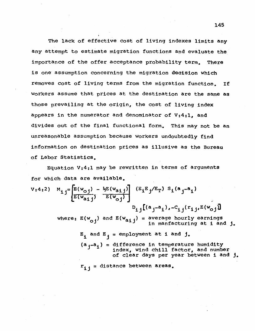
145
The lack of effective cost of living indexes limits any
any attempt to estimate migration functions and evaluate the
importance of the offer acceptance probability term, There
is one assumption concerning the migration decision which
removes cost of living terms from the migration function. If
workers assume that prices at the destination are the same as
those prevailing at the origin, the cost of living index
appears in the numerator and denominator of V:4:1, and
divides out of the final functional form, This may not be an
unreasonable assumption because workers undoubtedly find
information on destination prices as illusive as the Bureau
of Labor Statistics,
Equation V:4:1 may be rewritten in terms of arguments
for which data are available.
V:4:2) M _= E(w ) E(waij) (EiE J/ET) Si(a J-a i), E(waij E( wi
D j(aj-ai),-C i(rijE(wo i
where: E(wo ) and E(waij) = average hourly earningsin manfacturing at i and j.
E and E = employment at i and j.
(aj-ai) = difference in temperature humidityindex, wind chill factor, and numberof clear days per year between i and J.
r = distance between areas,
146
The basic relationship between the terms of the migration
function is multiplicative. If V:4:2 is to be written in
a form that can be made linear in its parameters, then the
internal form of the S and D functions must be multiplica-
tive.
V:4:3) s = Si(a J-a) = s0 (a j-a i)s
V:4:4) di= D (a -a ),-C (riE(w )
= d (a -a )dl (r )d2 (E(w ))d3
where: s , s*, d, d , d2' d3 are all parameters
Substituting these expressions for Si and D into V:4:2 and
adding parameters for offer acceptance probability and
employment, gives an expression that is linear in its loga-
rithms, which is shown in untransformed form below:
V:4:5)M =b s d E(w0 j) -3E(waij) bl(EE )b2(aj-ai) 1
(r )d2 (E(w
(ij) oj)d
The signs of all the constants and; in some cases the
magnitudes, have been developed previously. Only the
parameter which reflects the product of b , s , and d has not
received explicit attention. Actually this term may be great-
er than or equal to zero.
There is a final difficulty with the difference in
attractiveness terms, (a j-a i). This term may be negative
but that would leave the logarithmetic transformation
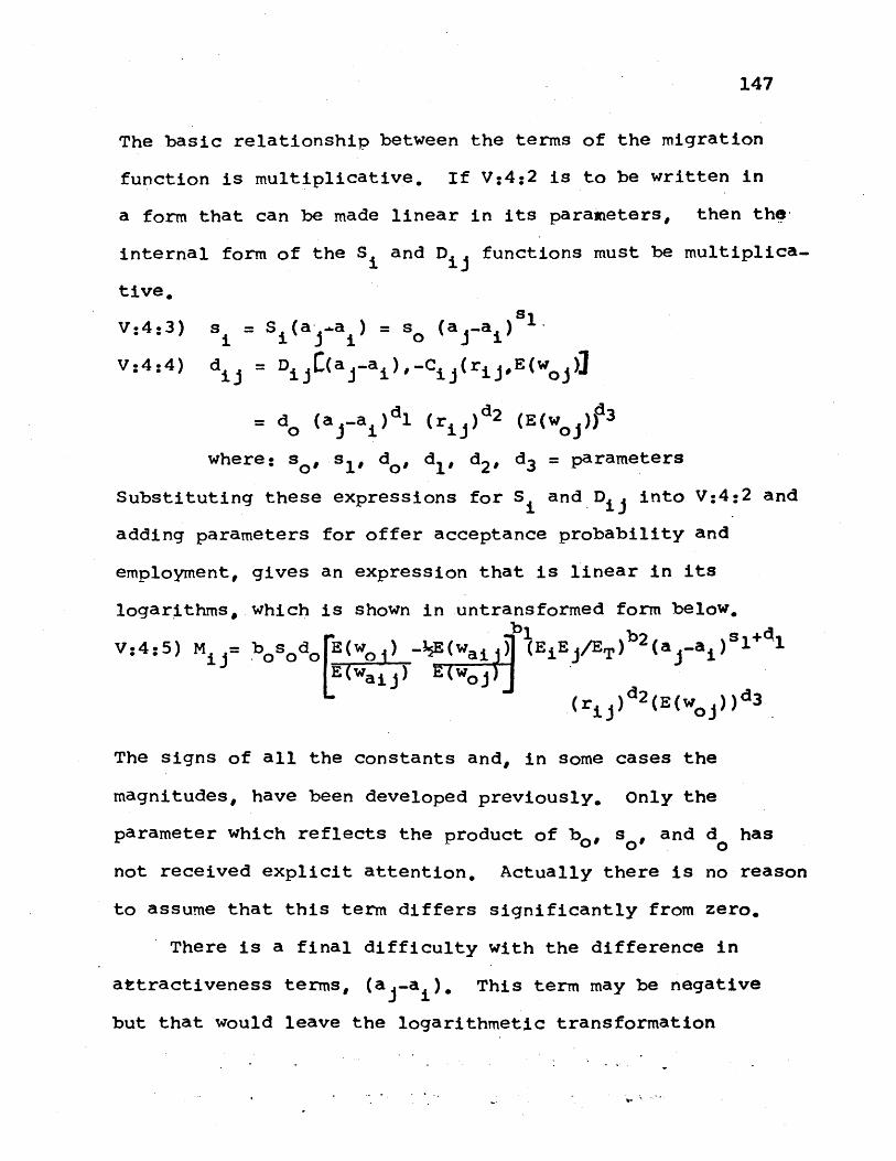
147
The basic relationship between the terms of the migration
function is multiplicative. If V:4:2 is to be written in
a form that can be made linear in its parameters, then the-
internal form of the S and D functions must be multiplica.
tive,
V:4:3) s = S (a- ..a) = s0 (a -a )l.
V:4:4) d = D j(a j-ai),-Ci(rijE(w0 Jl
=d (a a )dl (r d2 (E(w ))d3
where: so, sl, do, dl, d2, d3 = parameters
Substituting these expressions for S and-D into V:4:2 and
adding parameters for offer acceptance probability and
employment, gives an expression that is linear in its
logarithms, which is shown in untransformed form below,
V : 4 : 5 ) M = b o s o d o [ E )E Ei( b 2E / - a ) s l + d1
(waij) T -Woj)(r ii)d2(E(woi ))d3 .
The signs of all the constants and, in some cases the
magnitudes, have been developed previously. Only the
parameter which reflects the product of bo, so, and d has
not received explicit attention, Actually there is no reason
to assume that this term differs significantly from zero,
There is a final difficulty with the difference in
attractiveness terms, (a -a ). This term may be negative
but that would leave the logarithmetic transformation
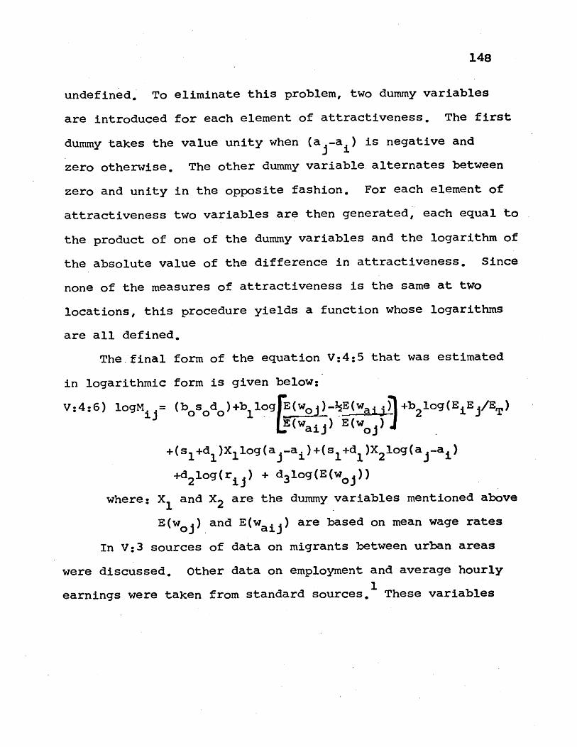
148
undefined. To eliminate this problem, two dummy variables
are introduced for each element of attractiveness. The first
dummy takes the value unity when (a -a ) is negative and
zero otherwise. The other dummy variable alternates between
zero and unity in the opposite fashion. For each element of
attractiveness two variables are then generated, each equal to
the product of one of the dummy variables and the logarithm of
the absolute value of the difference in attractiveness. Since
none of the measures of attractiveness is the same at two
locations, this procedure yields a function whose logarithms
are all defined.
The-final form of the equation V:4:5 that was estimated
in logarithmic form is given below:
V:4:6) logM = (b s d )+b log rE(woj)-kE(wai ) +b2 log(E EJ /ET)
(waij) E(w )
+(s 1+d 1 ) log(a J-a i)+(s 1+d 1 )21log(a J-a i)
+d2log(r ) + d3 log(E(w ))
where: X1 and X2 are the dummy variables mentioned above
E(w ) and E(w ) are based on mean wage rates
In V:3 sources of data on migrants between urban areas
were discussed. Other data on employment and average hourly
earnings were taken from standard sources. These variables
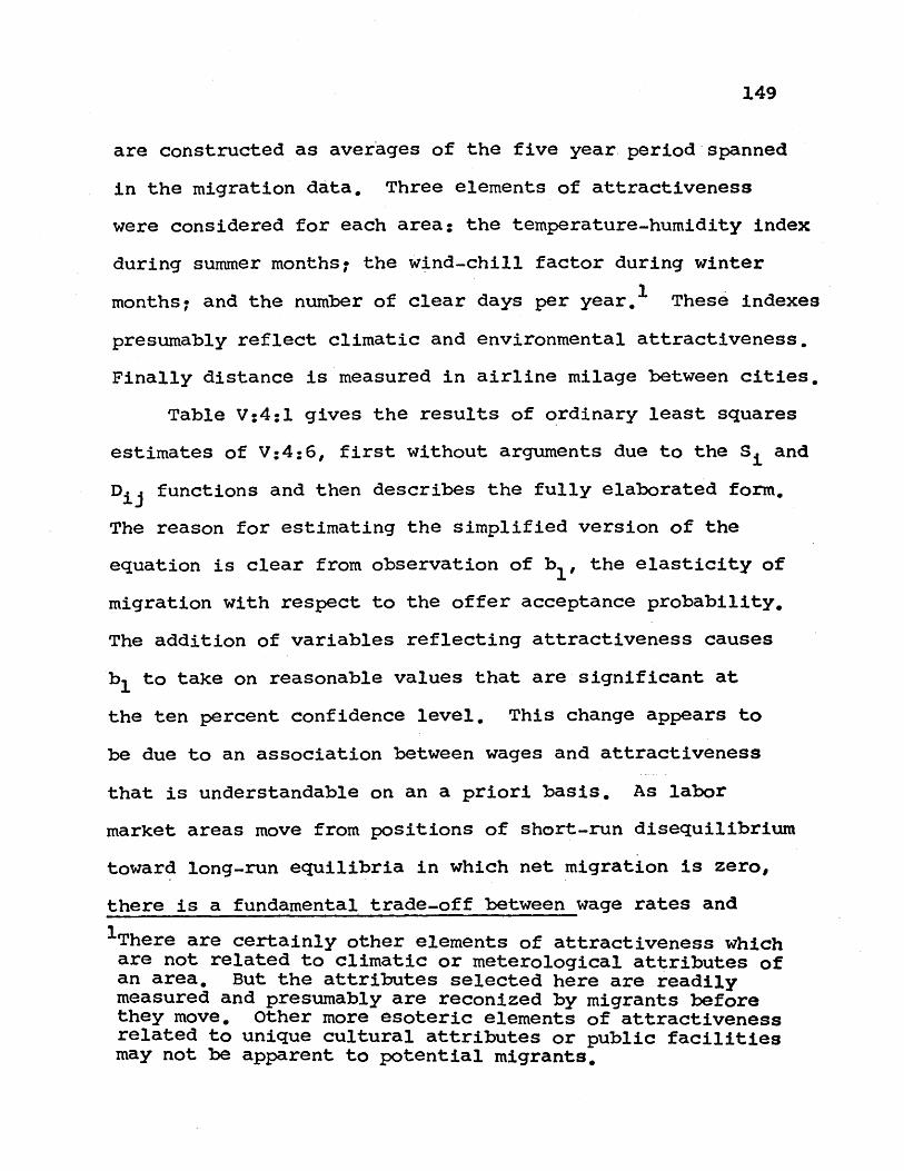
149
are constructed as averages of the five year period spanned
in the migration data. Three elements of attractiveness
were considered for each area: the temperature-humidity index
during summer months; the wind-chill factor during winter
months; and the number of clear days per year. These indexes
presumably reflect climatic and environmental attractiveness.
Finally distance is measured in airline milage between cities.
Table V:4:1 gives the results of ordinary least squares
estimates of V:4:6, first without arguments due to the Si and
Dij functions and then describes the fully elaborated form.
The reason for estimating the simplified version of the
equation is clear from observation of b1 , the elasticity of
migration with respect to the offer acceptance probability.
The addition of variables reflecting attractiveness causes
b to take on reasonable values that are significant at
the ten percent confidence level. This change appears to
be due to an association between wages and attractiveness
that is understandable on an a priori basis. As labor
market areas move from positions of short-run disequilibrium
toward long-run equilibria in which net migration is zero,
there is a fundamental trade-off between wage rates and
1There are certainly other elements of attractiveness whichare not related to climatic or meterological attributes ofan area. But the attributes selected here are readilymeasured and presumably are reconized by migrants beforethey move, other more esoteric elements of attractivenessrelated to unique cultural attributes or public facilitiesmay not be apparent to potential migrants.
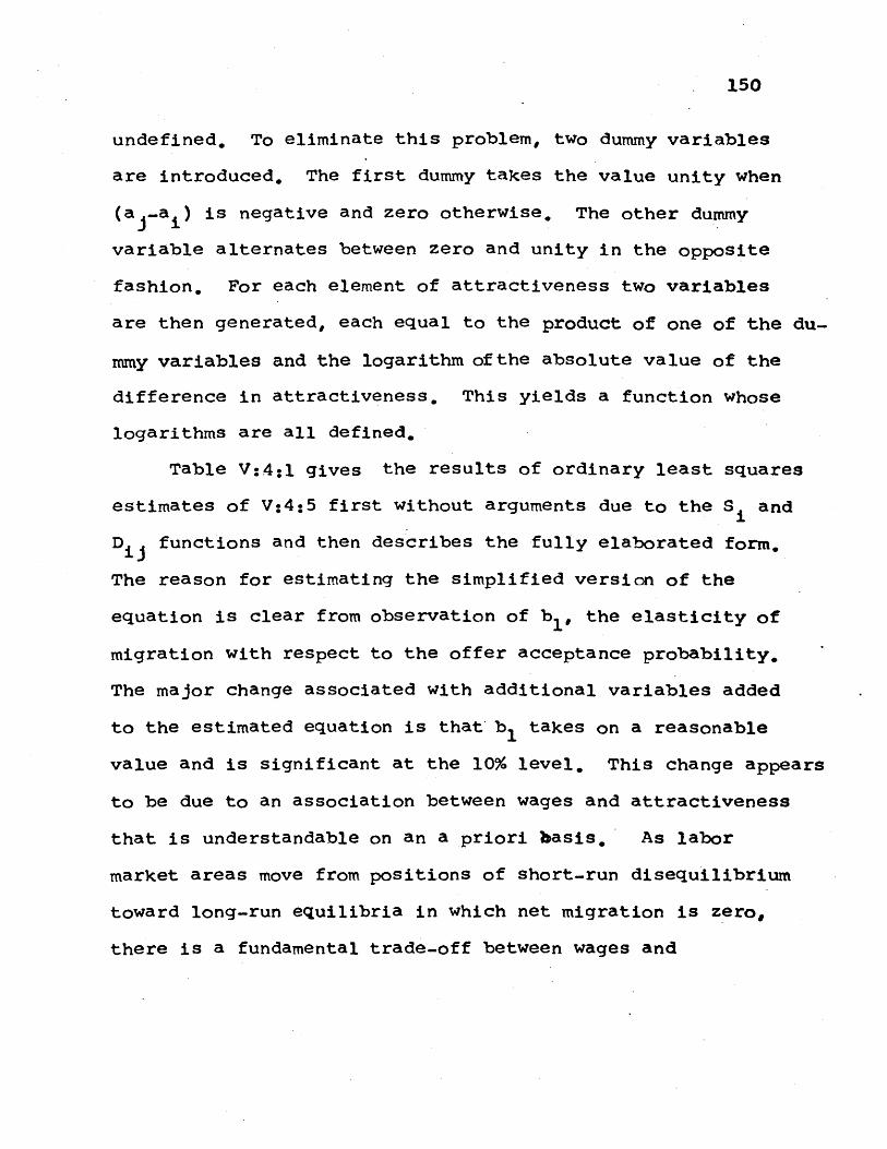
150
undefined. To eliminate this problem, two dummy variables
are introduced. The first dummy takes the value unity when
(a -aj) is negative and zero otherwise. The other dummy
variable alternates between zero and unity in the opposite
fashion, For each element of attractiveness two variables
are then generated, each equal to the product of one of the du-
mmy variables and the logarithm of the absolute value of the
difference in attractiveness, This yields a function whose
logarithms are all defined.
Table V:4:1 gives the results of ordinary least squares
estimates of V:4:5 first without arguments due to the Si and
D functions and then describes the fully elaborated form.
The reason for estimating the simplified version of the
equation is clear from observation of bl, the elasticity of
migration with respect to the offer acceptance probability.
The major change associated with additional variables added
to the estimated equation is that b takes on a reasonable1
value and is significant at the 10% level. This change appears
to be due to an association between wages and attractiveness
that is understandable on an a priori basis. As labor
market areas move from positions of short-run disequilibrium
toward long-run equilibria in which net migration is zero,
there is a fundamental trade-off between wages and
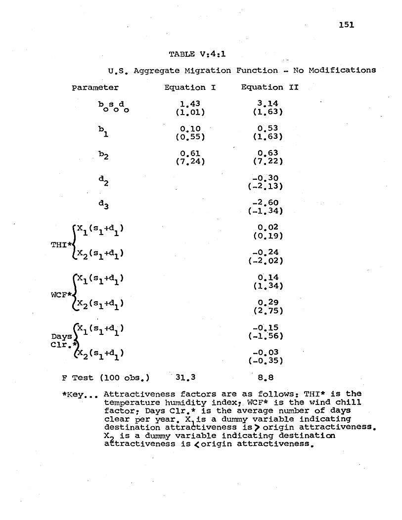
151
TABLE V:4:1
U.S. Aggregate Migration Function - No Modifications
parameter
b 0s 0d 0
b 1000
Equation I
1043(1.01)
0..10(0.55)
0.61(7024)
Equation
3.14(1.63)
0.53(1,63)
0.63(7,22)
-0.(-2
3013)
X1 (s +d )
THI*
X2(s 1 +d )
X 1 (s 1 +d)
WCF*
X2 (si+d1)
X (s +d)DaysClr.*
2(s 1 +d 1 )
F Test (100 obs.)
*Key...
-2.60(-1.34)
0,02(0.19)
-0.24(-2,02)
0014(1,34)
0.29(2,75)
-0.15(-1. 56)
-0,03(-0.35)
31,3 8.8
Attractiveness factors are as follows: THI* is thetemperature humidity index; WCF* is the wind chillfactor; Days Clr.* is the average number of daysclear per year, X is a dummy variable indicatingdestination attra tiveness is> origin attractiveness,X is a dummy variable indicating destinationaitractiveness is <origin attractiveness,
II
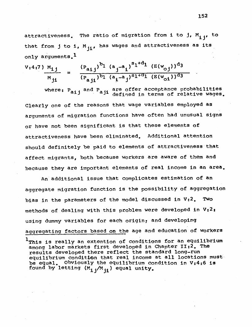
152
attractiveness, The ratio of migration from i to j, Mii, to
that from j to i1, M, has wages and attractiveness as its
only arguments. 1
V:4:7) Mu (p b1 (a a ) sl+dl (E(w ))d3
M (P )bl (a -a )sl+dl (E(woi))d3
where: p and P are offer acceptance probabilitiesaij aji defined in terms of relative wages.
Clearly one of the reasons that wage variables employed as
arguments of migration functions have often had unusual signs
or have not been significant is that these elements of
attractiveness have been eliminated. Additional attention
should definitely be paid to elements of attractiveness that
affect migrants, both because workers are aware of them and
because they are important elements of real income in an area,
An additional issue that complicates estimation of an
aggregate migration function is the possibility of aggregation
bias in the parameters of the model discussed in V:2. Two
methods of dealing with this problem were developed in V:2:
using dummy variables for each origin- and developing
aggregating factors based on the age and education of workers
This is really an extention of conditions for an equilibriumamong labor markets first developed in Chapter 11:2. Theresults developed there reflect the standard long-runequilibrium condition that real income at all locations must-be equal. Obviously the equilibrium condition in V:4:6 isfound by letting (M /Mu) equal unity.
153
at the origin. The difficulty with extensive use of dummy
variables is that such formulations ignore empirical informa.
tion on the nature of the population at the origin and that
dummies may be correlated with specific characteristics of
the origin that have nothing to do with aggregation problems.
Indeed this apparently was the case when a set of origin
dummies were used to estimate equations following the form
of V:4:6. The signs and significance of the coefficients of
offer acceptance probability associated with each origin
oscillated wildly.
Use of aggregating factors produced the improved results
indicated in Table V:4:2. The offer acceptance probability
term was multiplied by an aggregating factor identical to
that developed in equation V:2:7. In each case the factor
reflects the relative propensity of individuals at the origin
to move. This relative propensity was calculated first in
Table IV:2:1. The coefficient of this new adjusted aggregate
offer acceptance probability variable presented in Table V:4:2
is significant at the 5% level. This compares favorably to
the 10% confidence level applicable to the coefficient of
unadjusted offer acceptance probability presented in
Table V:4:1. Other parameter estimates differ little between
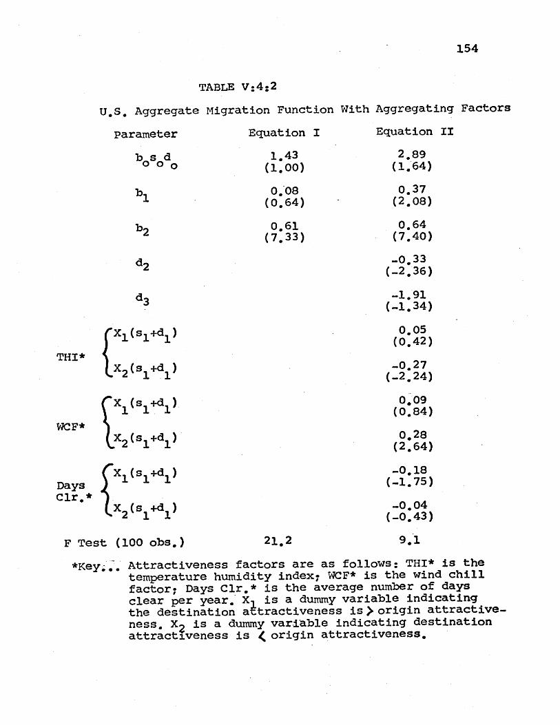
154
TABLE V:4:2
U.S. Aggregate Migration Function With Aggregating Factors
Parameter
bos 0d 0obod
Equation I
1.043(1.00)
0.08(0.64)
0.61(7.33)
Equation II
2.89(1.64)
0.37(2.08)
0.64(7.40)
-0.33(-2.36)
-1.91(-1.34)
X1 (s +d )
THI*X (s+d)2 1 1
X (s +d1 1
WCF*X (s 1 +d )
Days 5 X1 (s 1 +d )
Clr.* -
X (s +d )
F Test (100 obs.)
0.05(0.42)
-0.27(-2.24)
0.09(0.84)
0.28(2.64)
-0.18(-1-75)
-0.04(-0.43)
21,2 9.1
*Key- Attractiveness factors are as follows: THI* is thetemperature humidity index; WCF* is the wind chill
factor; Days Clr.* is the average number of daysclear per year. X is a dummy variable indicatingthe destination atractiveness is> origin attractive-
ness. X is a dummy variable indicating destinationattractiveness is ( origin attractiveness.
155
equation II in Table V:4:1 and equation IV in Table V:4:2.
There is an additional dimension to the aggregation
problem that must be considered. In V:2 the possibility of
aggregation bias in the variables as well as the parameters
of an aggregate migration function was developed. In this
case available data sources and a priori information are not
sufficient to provide schemes for consistent aggregation of
the arguments of an aggregate migration function. Thus the
use of average hourly earnings in the results presented earlier
may not lead to consistent aggregation. There is one mechanism
for evaluating the possible impact of aggregation bias in the
estimates given in Tables V:4:1 and V:4:2 This involves
estimating a migration equation based on an alternate wage
index, In this case the index is based on a random sample of
wages in specific occupations. The wage index is simply set
equal to the mean of these specific wages and not weighted by
the fraction of the total labor force in that occupation as is
the case with average earnings in manufacturing. Aggregation
problems arising in the wage variables are based on the notion
that the labor market is very compartmentalized with little
possibility of movement between occupations or industries., If
the labor market is sufficiently heterogeneous so that
156
aggregation bias is a significant problem, the use of an
unweighted wage index should produce results that differ
from those based on average hourly earnings in manufacturing.
Table V:4:3 presents estimates of the same equations
reported in Tables V:4:1 and V:4:2 with the unweighted wage
index substituted for average hourly earnings. There is
remarkably little difference between the estimates in Table
V:4:3 and those based on weighted wage indexes, Indeed the
estimate of b1 , the elasticity of migration with respect to
offer acceptance probability, in equation IV is 0,37 in
Table V:4:2 with a weighted wage index, and 0.41 in Table
V:4:3 where the unweighted index is used, Thus aggregation
bias in the wage variables appears to be of limited
importance.
The aggregate migration equation V:4:5 was also
estimated using data on migrants from the United Kingdom,
Unfortunately no data on attractiveness at various locations
was available and the earnings index was income per capita
rather than wages, However data on migrant flows is
available for two time periods,1959-1960 and 1965-1966.2
1other unweighted wage indexes were also tested with similarresults.
2The nature and sources of migration data were discussed isV:3.
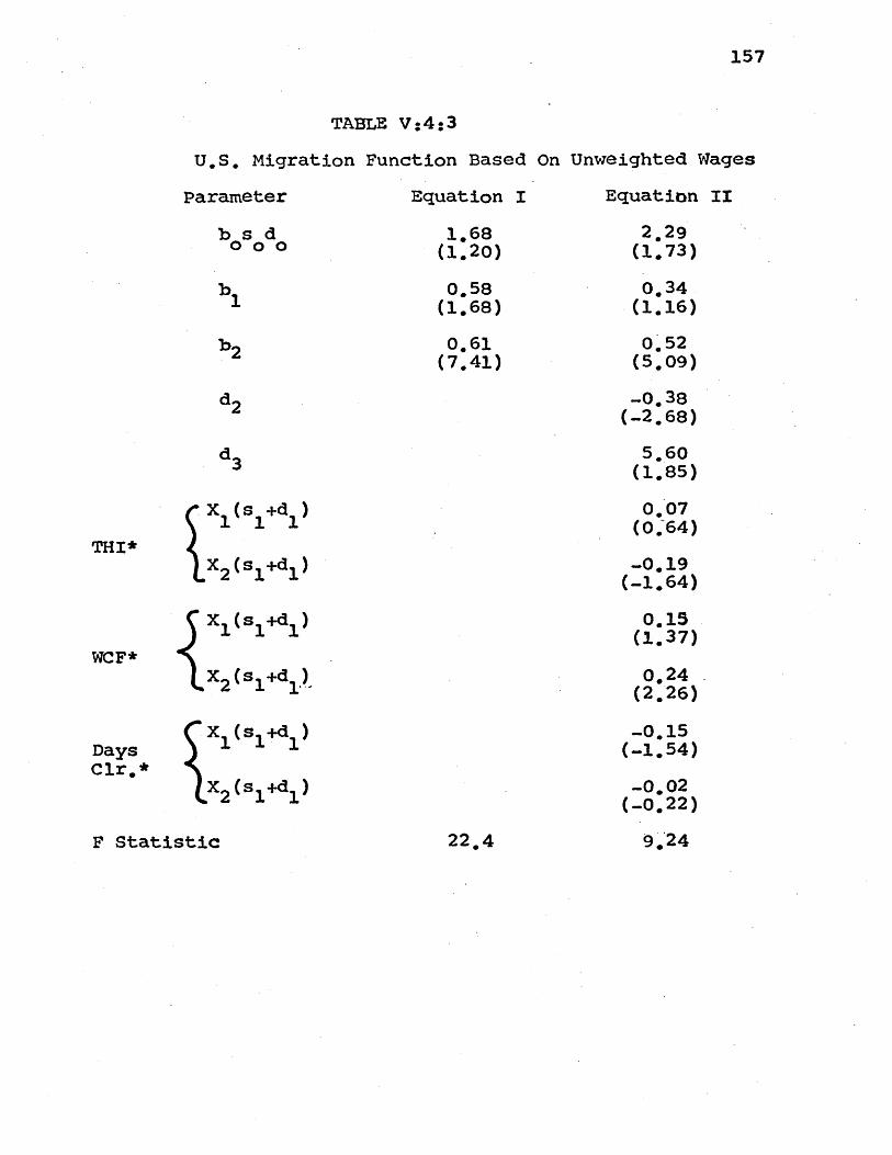
157
TABLE V:4:3
U.S. Migration Function Based On Unweighted Wages
Parameter
b s d0 0 0
Equation I
1068(1.20)
0.58(1.68)
0.61(7041)
Equation II
2029(1073)
0.34(1.16)
0.52(5.09)
X (s +da)
X2 (s 1 d1 )
X 1 (s 1 d)
WCF*X2(s M )
X (s
+d)
X2 (s 1+d 1)
F Statistic
THI*
-0.38(-2.68)
5.60(1.85)
0.07(0.64)
-0.19(-1.64)
0.15(1.37)
0.24(2.26)
-0.15(-1.54)
-0.02(-0.22)
DaysClr.*
22.4 9.24
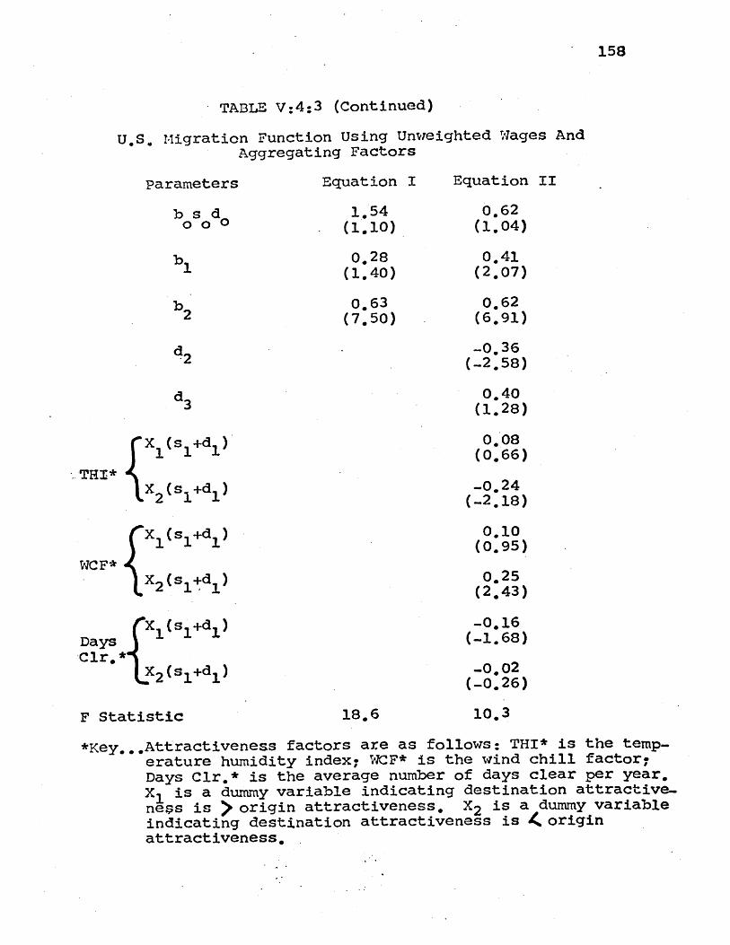
158
TABLE V:4:3 (Continued)
U.S. Migration Function Using Unweighted Wages AndAggregating Factors
Parameters
b os od 0bsd O
Equation I
1.54(1.10)
0.28(1.40)
0,63(7.50)
Equation II
0.62(1.04)
0*41(2.07)
0.62(6.91)
d.2
X 1(s 1+d)~
THI*X 2(s 1+d )
X (s +d )
WCF*
X 2(si +d)
Days X1(s1+dClr.*
X2 (sl+di)
F Statistic
-0.36(.2.58)
0.40(1.28)
0,08(0066)
-0.24(-2.18)
0.10(0.95)
0,25(2.43)
-0.16(-1.68)
-0.02(-0.26)
1806 10.3
*Key...Attractiveness factors are as follows: THI* is the temp-erature humidity index* WCF* is the wind chill factor7Days Clr.* is the average number of days clear per year,Xi is a dummy variable indicating destination attractive-ness is > origin attractiveness, X2 is a dummy variableindicating destination attractiveness is ( originattractiveness,
159
The availability of a time series of cross-section observations
of the dependent variable makes the use of dummy variables
for each origin reflect differences in propensity to
migrate, As was suggested in V:2, a set of dummy variables
was defined, one for each of six origins for which migration
data was available. Each variable takes on the value unity
when migrants eminate from a particular origin and zero
otherwise, A series of six offer acceptance probability
variables is then generated by multiplying each dummy by
the logarithm of offer acceptance probability calculated as
in V:4:5 using income per capita instead of wage data,
The estimated elasticity of migration with respect to
offer acceptance probability in Table V:4:4 is somewhat
higher than that found for the United States, Equation I,
which does not include a time dummy,(zero for 1960 and unity
for 1966), or the logarithm of destination wages, yields a
mean estimate of 1,22 for b1 , Equation II gives a mean of
1,67 for bl, but the logarithm of destination wages, or
income per capita which is used in lieu of wage data, is
inexplicably negative and significant,
Given the limitations imposed by data scarcity, the
discrepancies in estimates of b between models based on
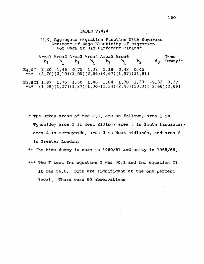
160
TABLE V:4:4
U.K. Aggregate Migration Function With SeparateEstimate of Wage Elasticity Of Migration
For Each Of Six Different Cities*
Areal Area2 Area3 Area4 Area5 Area6
b1 b 1 b 1 b 1b 1
Timed3 Dummy**
Eq.#I 2.20 1.46 0.75 1.32 1.18 0.42 0.45"t" (5.70)(3.10)(2.05)(3.66)(4.67)(1.97)(31.61)
Eq.#II 1.87 1.76 1.50 1.46 1.84 1.70 1.23 -9.32 3.37"t" (1.58)(1.27)(1.27)(1.30)(2.24)(2.43)(13.3)(-2.66)(2.69)
* The urban areas of the U.K. are as follows: area 1 is
Tyneside; area 2 is West Riding; area 3 is South Lancaster7
area 4 is Merseyside; area 6 is West Midlands; andaarea 6
is Greater London.
** The time dummy is zero in 1960/61 and unity in 1965/66.
*** The F test for equation I was 30.1 and for equation II
it was 56.6. Both are signifigant at the one percent
level. There were 60 observations
161
data from the United States and those using figures from the
United kingdom are not large, However, more thorough
validation and evaluation of aggregate migration functions
must wait upon the availability of more extensive data on
migrants between metropolitan areas,
162
Chapter VI
SUMMARY OF THE JOB-SEARCH MODEL OF MIGRATION
The task of this thesis, the derivation, specification,
and estimation of a job-search model of migration, has been
completed. The model developed here represents a significant
extention of the economics of information, and the body of
microeconomic theory. This chapter will first review these
innovations. Next implications for other results in the
literature on migration will be discussed. Finally
applications and suggestions for future research will be-'
reviewed.
VI:l) Contribution To Microeconomic Theory
The attempt has been made, where possible, to follow the
reasoning and notation common in the job-search literature.
For example, much of the analysis is based on the important
concept of an acceptance wage... But the acceptance wage
used f.n the migration model is based on a combination of
wages, search costs, and attractiveness. The ordinary job-
search models of individual labor markets do not consider
problems of relative attractiveness since this is constant
within a market area.
163
Similarly the concept of an offer-acceptance probability
1is not unknown in the job-search literature. Indeed within
a local labor market the acceptance wage determines the
probability that a wage chosen from the prevailing distribu-
tion will be accepted. This is not the case with the
model of migration. offer-acceptance probability varies
among destinations and is determined by a joint probability
density function of origin and destination wages. Thus the
analogy between job-search models and the migration model
developed here is based more on notation than substance.
One characteristic that is common to the migration model
and ordinary job-search models is consistency with assumptions
of microeconomic theory. Workers are attempting to maximize
the expected value of their real income. But they face
a distribution of earning- opportunities at each alternative
location, and positive costs of searching each opportunity.
If wages in each area were deterministic, the migration model
would yield the same sort of result as classic microeconomic
theory: offer-acceptance probability would be 1 or 0 depending
on the magnitude of origin and destination wages and migration
would follow to high wage areas where search was concentrated.
Similarly if search costs go to zero, the migration model
1Much of the notation and elements of the offer-acceptanceprobability concept used in this thesis is based on: Holt,Charles,"How To Alter The Relationship Between InflationAnd Unemployment In The U.S.,"(The Urban Institute),1970.
164
would yield the same results as classic microeconomic theory
since every area with wages higher than the origin would be
searched and the acceptance wage would be equal to the
maximum wage in any area.1 Indeed zero search cost is
equivalent to the notion of perfect information in micro-
economic theory since information is ubiquitous.
Useful additions needed to incorporate job-search models
of migration into a formal system of regional labor market
interactions would include a theory of firm behavior. This
is necessary to generate the distribution of offered wages
in each area as a function of search costs and labor turnover
costs. Completion of this element of analysis would emable
one to model the simultaneity between migration flows and
the demand for labor discussed in Chapter IV.
Empirical results from the estimated migration equations
indicate that migration is consistent with ordinary market
clearing processes. The coefficient of offer-acceptance
probability, b, was positive and significant in all
equations estimated in Chapter V. Since offer-acceptance
If wages are deterministic, then dW /dn is O for searchesbeyond one and by III:5:2 workers accept any offer abovepresent wages. Similarlyi if search costs are 0 then the6ct./an term in 111:5:2 is 0 and as long as there is anyincrease in wages associated with furthur search workerswill continue searching jobs - i.e. no wage below themaximum offered wage available will be accepted.
165
probability varies directly with destination wages and
inversely with origin-wages, the implied labor flows go from.
relatively low wage to high wage areas.
VI:2) Comparison With other Migration Functions
The job-search model of migration developed here is
more firmly grounded in microeconomic theory than approaches
based on "gravity" models reviewed in Chapter II. The
actual migration finally estimated in Chapter IV required
that an origin and destination wage distribution be assumed.
Given the assumed distributions, a unique functional form
suitable for estimation can be derived. However, the
functional form estimated here must be viewed as a special
case of the general migration function developed in
Chapter III.
There is some similarity between the functional form
of the job-search migration equation estimated ( equation
V:4:6 ) and other migration models in the literature. It
is common to find migration equation estimates that involve
the logarithm of the ratio of destination and origin wages,
or separate logarithms of destination and origin wages. As
stated in Chapter II, the result of this approach has been
to find only the logarithm of destination wages significantly
166
related to migration flows. The logarithm of wage ratio
variables and of origin wages is not found significant. This
has led to speculation that wages have a "pull" but not a
"push" effect on potential migrants. As an exercise the
migration data used in this study both from the U.S. and U.K.
were tested in migration equations involving all the
functional forms reviewed above: origin-destination wage
ratios; and origin and destination wage terms considered
separately. The results of other migration studies were
generally confirmed with wage ratios never proving significant
and individual wage terms generally insignificant and/or
possessing the wrong sign.
The job-search model of migration incorporates a
relative wage term in the offer-acceptance probability.
Estimates of the migration function show offer-acceptance
probability coefficients consistently significant with
signs indicating migration increases with destination wages
and decreases with origin wages. This means that there is
no paradox of "push" vs 'tpull" effects, but rather a basic
symmetry of wage effects- consistent with microeconomic theory.
The difference in empirical results associated with
substitution of the logarithm of offer-acceptance probability
for the logarithm of the wage ratio arises from a difference
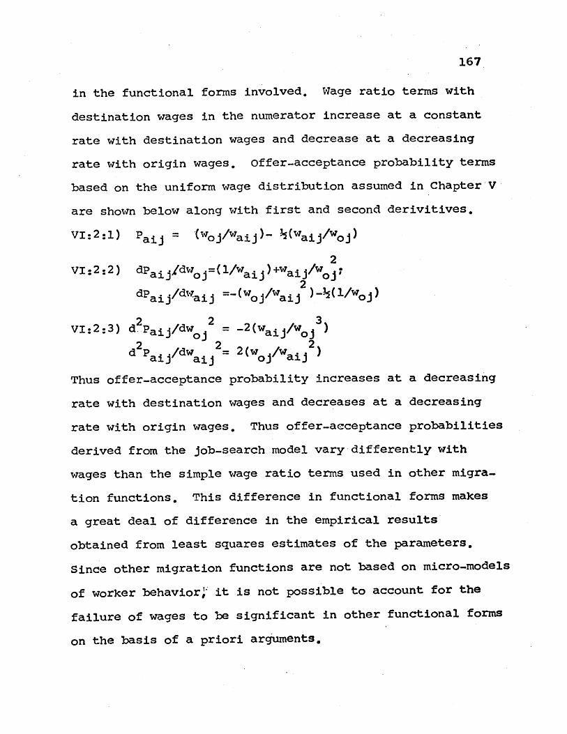
167
in the functional forms involved. Wage ratio terms with
destination wages in the numerator increase at a constant
rate with destination wages and decrease at a decreasing
rate with origin wages. offer-acceptance probability terms
based on the uniform wage distribution assumed in Chapter V
are shown below along with first and second derivitives.
VI:2:1) Paij (woj/waij)- (waij/woj)
2VI:2:2) dPajdw (1/Wa*)+waij/w
2 3VI:2:3) d2Paij/dw = -2(waij/wo)d.Pai/dwo
d Paij /dwaij w /waij
Thus offer-acceptance probability increases at a decreasing
rate with destination wages and decreases at a decreasing
rate with origin wages. Thus offer-acceptance probabilities
derived from the job-search model vary differently with
wages than the simple wage ratio terms used in other migra-
tion functions. This difference in functional forms makes
a great deal of difference in the empirical results
obtained from least squares estimates of the parameters.
Since other migration functions are not based on micro-models
of worker behavior' it is not possible to account for the
failure of wages to be significant in other functional forms
on the basis of a priori arguments.
168
While the job-search model of migration represents an
important departure from previous analytical approaches to
migration, the job-search is consistent with much of the
other literature reviewed, Indeed the approach taken in
this thesis was suggested by an extensive examination of
survey research on migrants. Workers consistently report
a migration decision based on limited information with
target or acceptance wage goals,
Similarly the job-search approach is consistent with
descriptive studies of historic migration movements. Such
classical results as the tendency of flows in one direction
to generate reverse flows are explained by the tendency of
individuals to search in their former home area and the
notion of an offer-acceptance probability based on origin
wages. Thus workers may accept a position in what appears to
be a lower wage area provided that the offered wage is above
the relevent acceptance wage, This kind of consistency
with survey literature and descriptive studies perhaps
provides a stronger confirmation of job-search approaches
than any other piece of empirical evidence,
169
APPENDIX Al
As was established in the introduction, migration equa-
tions often play a most important role in models of regional
and urban growth. Undoubtedly the most controversial of
1these models is Urban Dynamics. This appendix will show
that the behavior of the urban dynamics model is dominated
by its migration equations and that a more reasonable
specification of these equations alters the behavior of the
model significantly.
The urban dynamics model is a continuous simulation of
strictly recursive difference equations connecting 20 state
variables. These variables completely characterize the
city at any time and are chosei to reflect the major compon-
ents of an urban environment: housing? land, whose total area
is fixed7 employment or industry. and population. The model
has not been fitted to a particular urban area. It is
designed to fit an area large enough to contain a labor and
housing market but constrained in size by features of access-
ibility, topography, and/or political fiat (e.g. a greenbelt).
Although none of the variables in Urban Dynamics is
operationally defined, they have an intuitive appeal to anyone
familiar with the popular literature on "the urban problem."
population is divided into manager, labor, and underemployed
1 Forrester, Jay W., Urban Dynamics, (Cambridge, Massachusetts:M.I.T. Press), 1969.

170
groups, presumably based on socio-economic status. Three
grades of housing are distinguished: premium; worker; and
slum housing, reflecting the housing budget of the three
population groups. The three kinds of industry - new
enterprise, mature enterprise, and declining industry -
employ different mixes of the three population types with
total labor per enterprise declining with age. Since output
per worker and land area per worker is generally larger in
newer plants, thus empirical evidence suggests that declining
industry might have more workers per unit land area. But
simulation experiments have shown that the parameters govern-
ing labor input per type of enterprise have little effect on
model behavior. Indeed this insentivity characterizes the
response of the urban dynamics model to changes in most
individual parameters.
The urban dynamics model reaches an apparently steady
state for most reasonable initial vlaues of the state varia-
bles. This equilibrium is due in large part to the fixed
land area and the discouraging effect which increasing gross
densities have on all forms of activity within the city.
The steady state of the urban dynamics model is chara-
cterized by stable values for population and its three
components. Such population stability implies balance
between the forces tending to change population levels:

171
in-migration; out-migration7 upward social mobility: downward
social mobility7 and net natural increase. Each demographic
group sires only offspring of its own kind and marriage
between classes Is forbidden. Such assumptions violate "the
American dream" and perhaps reality as well. Social mobility
depends on job opportunities in different labor markets, and
on public expenditures, presumably on retraining and educa-
tion.
The migration equations of Urban Dynamics are formulated
so that people move in response to the condition of the city
relative to an unchanging environment.
"For any class of person, conditions in the area must beapproximately equal in attractiveness to conditions else-where. As an example, conditions in a city for people inthe lowest economic class will not be substantially betteror worse than the conditions in other parts of the countryfrom which there is free mobility." 1
Thus the proper indicator of success for the city is its
ability to achieve a given mix of attractiveness factors
relative to the unchanging environment. Attractiveness
consists of many factors.
"Attractiveness is a multidimensional concept and includesfactors such as legal restrictions, prejudice, racial andethnic groupings, and anything else that influences aperson to move. Some of these are represented explicitlyin the urban model. All others are combined into themobility coefficients on the basis that they can betreated as constants and are not involved as dynamic 2variables in the modes of urban change here explored."
Components of relative attractive attractiveness are imbedded
1 Forrester, Jay, ibid., pg 117,2 Forrester, Jay, ibid., pg. 118.
172
in the constants of the migration function and in the few
state variables generated endogensously by the model.
There are separate in and out-migration equations for
each population group. The migration equations for the
underemployed are most ±mportant and have the following
form:
AI:l) UA = (U+L) (UAN) (AMMP)
AI:2) UD = U (UDN) (UDM)
where: UA = underemployed arrivals per unit time
UD = underemployed departures per unit time
U = number of underemployed in the city
L = number of laborers (workers) in the city
UAN = "normal" underemployedarrivals rate = .05
AMMP = relative attractiveness for migration
UDN = "normal" underemployed departure rate =*02
UDM = relatiVOeunattrctiieness for migration
The constant factors mentioned above are embodied in the con-
stants UAN and UDN. The (U+L) and U termsin equations AI:1
and AI:2 respectively, are justified as scaling factors. In
the steady state there is an inverse relationship between
relative attractiveness, AMMP, and unattractiveness, UDM.
AI:3) AMMP = AMM = (UDM)
where: AMM = attractiveness for migration multiplier(relative cattractiveness of the city)
Forrester, Jay, ibid., pg. 135.
173
If there were no natural increase or social mobility, the
steady state would be characterized by an equality of arrivals
and departures.
AI:4) UA = (U+L) .05 (AMM) = UD = U .02 (AMM)Y
Solving for AMM, we find that it must be less than one.
AI:5) AMM = C *02 U/.05 (U+L) 3 ( 1
In the case of both laborers and managers the scaling factors
for in and out-migration are. identical. Thus when similar
expressions to AI7 5 are derived for attractiveness to laborers
(LAM) and to managers (MAM), the scaling factors cancel out
and exact numerical values can be obtained for relative
attractiveness.
AI:6) LAM = ( LDN L/LAN L ) = (.02/.03) = 0.815
AI:7) MAM = ( MDN M/MAN M )h = (.02/.03)1 = 0.815
Where: LAM = relative attractiveness for migrationto laborers
LDN = "normal" labor departure rate = .02
LAN = "normal" labor arrival rate = .03
MAM = relative attractiveness for migrationto managers
MDN = "normal" manager departure rate = .02
MAN = "normal" manager arrival rate = .03
In all cases relative attractiveness, as indicated by AMM,
LAM, and MAM, in the city is below that in the environment.
The addition of net natural increase, modeled as a proportion-
al increase in each population type, only lowers the relative
174
attractiveness of the city furthur, since even more -people
must be induced to emigrate each year. As compared to zero
net migration in the case analyzed above, with net population
increase steady state migration must produce net outflows
equal to the population increase.
The effect of population growth and social mobility on
relative attractiveness of the city can be analyzed by writ-
ing the equations for total change in each population group.,(Chage)=In-mira '+ Soc at)
(Change)=(In-migration)-(Out-migration)+(Increase)l.(Mobity)
AI:8) DU = .05(U+L)(AMM) - .02(AMM)~ + (UB) + (LTU) - (UTL)
AI:9) DL = .03 L (LAM) - .02(LAM)~ + (LB)a(LTM)-(LTU)+ (UTL)
AI:l0)DM = .03 M (MAM) - .02(MAM)O+ (MB)+(LTM)
where: DU = net change in underemployed population per year
DL = net change in labor population per year
DM = net change in manager population per year
UB, LB, MB = net natural increase per year of under-underemployed, laborers, and managers respect.ively
UTL = mobility of underemployed to labor category
LTU = mobility of laborers to underemployed category
LTM = mobility of laborers to manager category.
The steady state is characterized by stable levels of all
population groups, DM = DL = DU = DP = 0. Adding equations
AI:8, AI:9, and AI:l0, gives an expression for population
change, DP, involving only attractiveness and natural
175
increase.
AI:ll) DP = .05(U+L)(AMM)-.02(AMM)-"+ UB +.03L(LAM)-.02L(LAM)~
+ LB + .03M(MAM)-.02M(MAM)-1 + MB = 0
In equation AI:ll, DP varies directly with all three attrac-.
tiveness multipliers, AM, LAM, and MAM, and with the three
natural increase variables, UB, LB, and MB. Thus there is
a fundamental tradeoff between all six of-these variables. Any
rise in rates of natural increase lowers attractiveness as
was asserted above. Similarly improving attractiveness to one
group will result in lower attractiveness to other groups if
natural increase is constant. 1
Inherint in the nature of the attractiveness functions,
AMM, LAM, and MAM, is the immutability of their parameters
which reflect individual tastes and the constant environment.
While the policy-maker has control over the parameters that
affect the steady-state values of the arguments of the
attractiveness function, he cannot control the total attrac-
tiveness associated with a given menue of arguments of the
attractiveness function. Temporary increases (decreases) in
attractiveness to a particular group are quickly wiped out by
increases (decreases) in the relevent population types that
reduce the attractiveness of the area.
Formalizing this argument, we have found that (dAMM/dMAM)DPOand (dAMM/dLAM)DP=O and (dLAM/dMAM)DP=o are all negative.
176
The inability to change total attractiveness is illustra-
ted admirably by Table AI:I which shows the population and
attractiveness of the city in its "stagnant" steady state and
Professor Forrester's favorite urban renewal policy: slum
housing demolition and new enterprise construction.
TABLE AI:1
Attractiveness Under "Stagnation" And "Revival"
"Stagnation" Variable Name "Urban Revival"
0.449 AMM 0.428
0.625 IAM 0.611
0.307 MAM 0.297
377,300 U 335,900
392,600 L 600,000
71.100 M 108.700
The revived city has more population living at uniformly
lower levels of average attractiveness. All three attrac-
tiveness multipliers are lower because with the rise in
population annual net population increase is larger. The city
must be less attractive in order to induce net out migration
equal to natural increase. Equation AI:ll shown the inverse
relationship between attractiveness and population increase.
The revival policy adjusts components of attractiveness, trad.
ing off housing for employment and tax base. Because these
three important variables are linked in the attractiveness
functions, it is impossible to find the classic match of
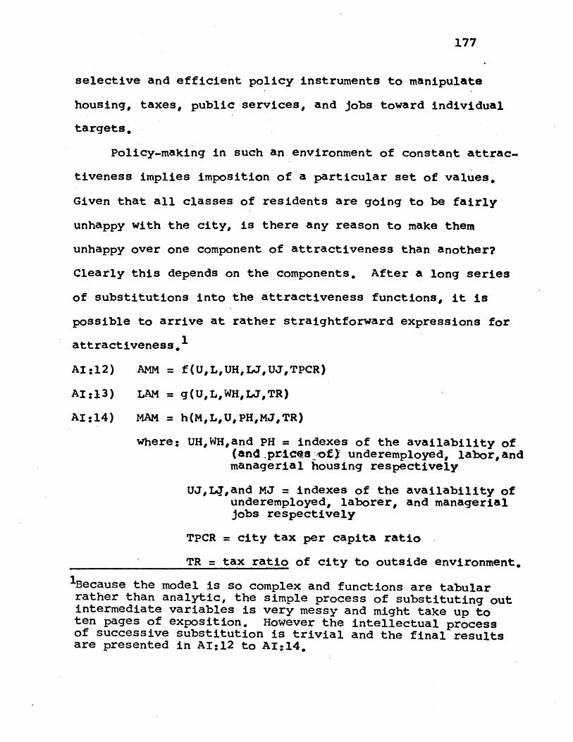
177
selective and efficient policy instruments to manipulate
housing, taxes, public services, and jobs toward individual
targets,
Policy-making in such an environment of constant attrac-
tiveness implies imposition of a particular set of values,
Given that all classes of residents are ging to be fairly
unhappy with the city, is there any reason to make them
unhappy over one component of attractiveness than another?
Clearly this depends on the components, After a long series
of substitutions into the attractiveness functions, it is
possible to arrive at rather straightforward expressions for
attractiveness,
AI:12) AMM = f(U,L,UH,LJ,UJ,TPCR)
AI:13) LAM = g(U,L,WH,LJ,TR)
AI:14) MAM = h(ML,U,PHMJ, TR)
where: UH,WH,and PH = indexes of the availability of(and pries/ofY underemployed, labor, andmanagerial housing respectively
UJ,LJ,and MJ = indexes of the availability ofunderemployed, laborer, and managerialjobs respectively
TPCR = city tax per capita ratio
TR = tax ratio of city to outside environment,
1Because the model is so complex and functions are tabularrather than analytic, the simple process of substituting outintermediate variables is very messy and might take up toten pages of exposition. However the intellectual processof successive substitution is trivial and the final resultsare presented in AI:12 to AI:14.
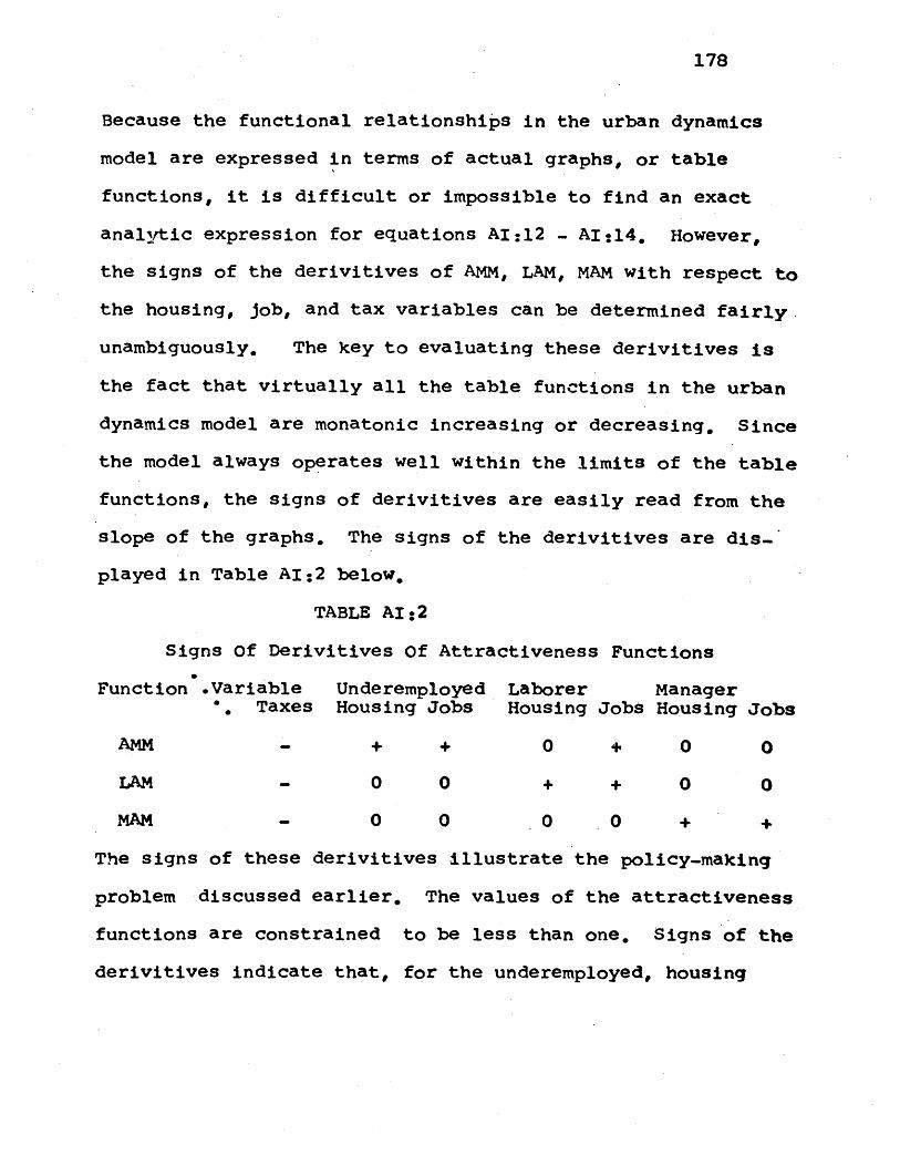
178
Because the functional relationships in the urban dynamics
model are expressed in terms of actual graphs, or table
functions, it is difficult or impossible to find an exact
analytic expression for equations AI:12 - AI:14. However,
the signs of the derivitives of AMM, LAM, MAM with respect to
the housing, job, and tax variables can be determined fairly.
unambiguously. The key to evaluating these derivitives is
the fact that virtually all the table functions in the urban
dynamics model are monatonic increasing or decreasing. Since
the model always operates well within the limits of the table
functions, the signs of derivitives are easily read from the
slope of the graphs. The signs of the derivitives are dis..
played in Table AI:2 below.
TABLE AI:2
Signs Of Derivitives Of Attractiveness Functions
Function .Variable Underemployed Laborer Manager. Taxes Housing Jobs Housing Jobs Housing Jobs
AMM - + + 0 + 0 0
LAM 0 0 + + 0 0
MAM - 0 0 0 0 + +
The signs of these derivitives illustrate the policy-making
problem discussed earlier. The values of the attractiveness
functions are constrained to be less than one. Signs of the
derivitives indicate that, for the underemployed, housing
179
availability can only be increased at the expense of job
availabiity or tax increases. Similar results hold for
other population groups.
Whether Urban Dynamics is viewed as an accurate represen-
tation of city growth processes or not, the most important
result of this inquiry is the importance of the migration
equations to the urban dynamics model, and particularly to
policy conclusions based on the model. Indeed the migration
equations contain information on the fundamental long-run
tradeoffs facing the city. The variables determining attrac-
tiveness of an area for migration reflect desires of the
population for the quality of urban life. Such desires are
the proper concern of public officials. This is the key to
the importance of migration functions to any policy-oriented
model of urban development.
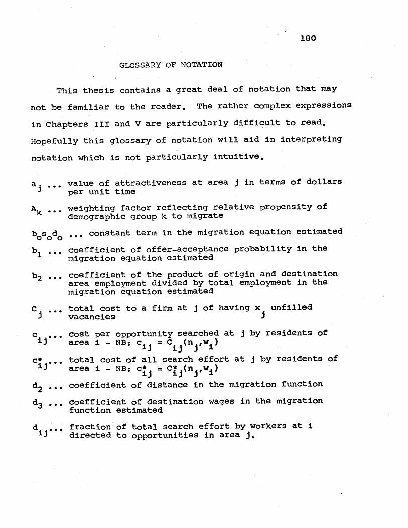
180
GLOSSARY OF NOTATION
This thesis contains a great deal of notation that may
not be familiar to the reader. The rather complex expressions
in Chapters III and V are particularly difficult to read,
Hopefully this glossary of notation will aid in interpreting
notation which is not particularly intuitive,
a ... value of attractiveness at area j in terms of dollarsper unit time
A ... weighting factor reflecting relative propensity ofdemographic group k to migrate
bosod ... constant term in the migration equation estimated
b . coefficient of offer-acceptance probability in themigration equation estimated
b2-- coefficient of the product of origin and destinationarea employment divided by total employment in themigration equation estimated
C ... total cost to a firm at j of having x unfilledI vacancies
c . cost per opportunity searched at j by residents ofiJ* area i - NB: cii = C (n ,w
c* ... total cost of all search effort at j by residents ofarea i - NB: c* = C* (n ,w
d2 ** coefficient of distance in the migration function
d3 **coefficient of destination wages in the migrationfunction estimated
d .. 0 fraction of total search effort by workers at idirected to opportunities in area j.
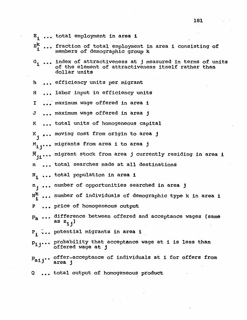
181
E ... total employment in area i
Ek ... fraction of total employment in area i consisting ofmembers of demographic group k
G ... index of attractiveness at j measured in terms of unitsof the element of attractiveness itself rather thandollar units
h ... efficiency units per migrant
H ... labor input in efficiency units
I .. maximum wage offered in area i
J ... maximum wage offered in area j
K ... total units of homogeneous capital
K ,.. moving cost from origin to area J
M . . .migrants from area i to area j
M ... migrant stock from area j currently residing in area i
n *.. total searches made at all destinations
N 0.. total population in area i
n ... number of opportunities searched in area j
Nk .. number of individuals cf demographic type k in area ii
p .. price of homogeneous output
Pa'' difference between offered and acceptance wages (sameas z ij)
p .* potential migrants in area ii
p . . . probability that acceptance wage at i is less thanoffered wage at j
pa..O offer-acceptance of individuals at i for offers fromarea j
Q .. total output of homogeneous product
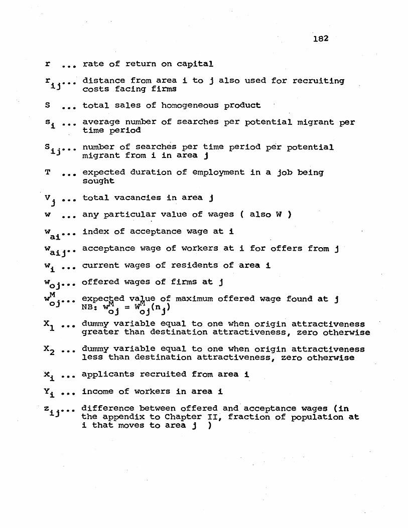
182
r .. rate of return on capital
r . distance from area i to j also used for recruitingcosts facing firms
S .. * total sales of homogeneous product
s ... average number of searches per potential migrant pertime period
S ... 0 number of searches per time period per potentialmigrant from i in area j
T *.. expected duration of employment in a job beingsought
V ... total vacancies in area j
w .. any particular value of wages ( also W )
W ai. index of acceptance wage at i
w acceptance wage of workers at i for offers from jaijOO
w .000current wages of residents of area i
weg... offered wages of firms at j
N.... expe ed va ue of maximum offered wage found at j0 NB:WM = (n)
oj oj y
X . . . dummy variable equal to one when origin attractivenessgreater than destination attractiveness, zero otherwise
X2 *00 *dummy variable equal to one when origin attractivenessless than destination attractiveness, zero otherwise
it ... applicants recruited from area i
Yi ... income of workers in area i
z .. 00difference between offered and acceptance wages (inthe appendix to Chapter II, fraction of population ati that moves to area j )