of J. Math. Biol. (1989) 27:117-138 Biologyeebweb.arizona.edu/Faculty/chesson/Peter/Reprints/1989_Invasibility... · J. Math. Biol. (1989) 27:117-138 ,Journal of Mathematical Biology

J. Math. Biol. (1989) 27:117-138 ,Journal of

Mathematical Biology

�9 Springer-Verlag 1989

Invasibility and stochastic boundedness in monotonic competition models

P. L. Chesson I and S. Ellner 2

i Department of Zoology, Ohio State University, 1735 Neil Avenue, Columbus, OH 43210, USA 2 Biomathematics Graduate Program, Department of Statistics, Box 8203, North Carolina State University, Raleigh, NC 27695, USA

Abstract. We give necessary and sufficient conditions for stochastically bounded coexistence in a class of models for two species competing in a randomly varying environment. Coexistence is implied by mutual invasibility, as conjectured by Turelli. In the absence of invasibility, a species converges to extinction with large probability if its initial population is small, and extinction of one species must occur with probability one regardless of the initial population sizes. These results are applied to a general symmetric competition model to find conditions under which environmental fluctuations imply coexistence or competitive exclusion.

Key words: Invasibility - - Stochastic boundedness - - Competition - - Coexistence - - Competitive exclusion

I. Introduction

In recent years there has been much interest in modeling populations and communities in stochastically fluctuating environments (May 1974; Slatkin 1978; Turelli 1977, 1980, 1981; Chesson 1982, 1986; Ellner 1984; Abrams 1984; Shmida and Ellner 1985). Simultaneously, there has been a rise in empirical evidence that such environmental fluctuations have an important effect on population dynamics and community structure (Grubb 1977; Sale 1977; Connell and Sousa 1983; Underwood and Denley 1984; Murdoch et al. 1985; Strong 1986). In the modeling efforts, a fundamental problem has arisen: how does one determine whether a population or a genotype persists, or whether the species in a community coexist? This problem has two parts: first defining persistence and coexistence, and second finding ways of demonstrating such persistence or coexistence. In models with a continuous state space, persistence is usually defined in terms of the behavior of the probability distribution of population size as time goes to infinity (Turelli 1977, 1981).

118 P.L. Chesson and S. Ellner

Commonly, a species has been regarded as persisting if the probability distribution of population size converges to that of a positive random variable. However, Chesson (1978, 1982) suggested that this requirement is too strict and proposed a weaker requirement, the stochastic boundedness criterion, which simply requires the distribution of population size to be bounded below by that of a positive random variable. There are few useful results permitting either of these two persistence conditions to be established for multispecies population models. Consequently, many workers have used the yet weaker criterion "invasibility" (Turelli 1978). This criterion relies on the fact that if the geometric-mean growth rate of a species at low density is greater than 1, the species can increase from low density. Hence it recovers from low density or "invades" the system. The invasibility criterion is not regarded as a satisfactory criterion by itself, but is often presumed to imply stochastic boundedness. Rigorous mathematical demonstrations are available for a variety of one-dimensional models (Norman 1976; Chesson 1982; Ellner 1984), but it is known not to apply in all cases (Chesson 1982). There are some results for continuous-time two-dimensional models (Turelli and Gillespie 1980), but results for the corresponding discrete- time models are lacking. Strong support for the idea that invasibility broadly implies stochastic boundedness comes from computer simulations (Turelli 1980; Ellner 1985).

In this article we show that invasibility implies stochastic boundedness in a class of two-dimensional two-species competition models described by stochastic difference equations. We show that if each species can invade the system in the presence of the other species, the species coexist in the sense that each is stochastically boundedly persistent. We then go on to examine cases where the invasibility criterion does not hold, and show that a.s. convergence of one species to 0 is to be expected. The main assumptions imposed on the model are monotonicity and independence of the environmental states at different times.

Assumptions and results are given in Sects. 2 and 3. Section 4 applies these results to a general symmetric competition model. The proofs are in Sect. 5.

2. Sufficient conditions for coexistence

We consider the discrete-time competition process (X1,3(2)={(Xl( t ) , X2(t)), t =0, 1 , . . . ) , where the nonnegative random variable X~(t) is the population density of species i at time t. The competition process is dependent on an environment process {~(t)}, which takes values in some measurable space. The dynamics of the system are governed by the following equation

X,( t + 1) = Fi(X~(t), Xj(t), ~(1)), (2.1)

where here, and in the sequel, (i , j) can take only the values (1, 2) and (2, 1). The functions Fi are nonnegative and jointly measurable in their three arguments. We assume that the system is closed to immigration and therefore that Fi can be written in the form

F,(x,, xj, ~) = x,f,(xi, xj, ~). (2.2)

lnvasibility and stochastic boundedness 119

Assumptions below allow f ( 0 , xj, ge) to be defined as the limit as xi ~ 0 of f (x i , x~, ~). While this quantity may be infinite, we assume that F~(0, x:, ~g) = O.

To derive necessary conditions for coexistence, we need to make a number of assumptions. Some of these, stated as A1, A2, A3, below, are mathematical technicalities, but we also make several biologically meaningful assumptions that indicate the circumstances for which our results are applicable.

The first assumption is that the environment process {~(t)}~=o is a sequence of independent and identically distributed random variables. This is the standard white-noise environment for discrete time, and it implies that (X1,X2) is a homogeneous Markov process. While this environment assumption rules out environmental correlations between years, correlations among components of the environment process within years are certainly permitted. For example, if ~ ( t ) = (~ l ( t ) , ~ 2 ( t ) , . . . , ~n(t)), there is no assumption of independence between ~u(t) and ~v(t), for any u, v..

The second assumption, which is implicit in Eq. (2.1), is that the state of each population is completely described by the population density (number of individuals per unit area). Any characteristics that vary among individuals, such as age, size, location, or genotype are assumed to be unimportant for population dynamics, or if important they are assumed to have a distribution within the population that can be expressed as a function of the population density and the environment at a given time. Under these general circumstances, Prout and McChesney (1985) and Prout (1986) have pointed out that an equation like (2.1) may yet only apply to the population density of one particular stage in the life cycle. For our purposes, this is not a problem because a population becomes extinct if- and only if all stages in the life cycle become extinct.

The final biologically important assumption is monotonicity of the competitive effects. We assume throughout that each F~(x~, x:, ~) is nondecreasing in x~ and xj, and positive whenever xi > 0. The monotonicity in x~ simply says that competition occurs. Competition between species could be asymmetrical; in particular, our assumptions permit amensalism. Monotonicity in xi implies that intraspecific competition is never so severe that a higher density now means a lower density after one unit of time. This situation is sometimes referred to as contest competition as opposed to "scramble" competition. It implies that the corresponding single-species models have very simple dynamics: monotonic convergence to a stable equilibrium. Some authors have suggested that in a constant environment many natural populations would have stable equilibria in accordance with our assumptions (Tanner 1975; May 1981, Chaps. 2 and 5). However, Schaffer and Kot (1986), discuss evidence suggesting that more complicated dynamics under constant environment conditions may often occur, imposing a genuine restriction on the applicability of our results.

A simple model violating our assumption ofmonotonici ty of (2.1) in x; involves variable recruitment to an adult population according to the Ricker formula. Population dynamics in this model are expressed as

Xi( t + 1) -- siX,( t ) + r~( t ) Xi( t ) exp{ - [ Xi( t ) + a:Xj (t)]}.

Here the c~'s and s's are positive constants, and the r~(t) represent the environment process ~. The first term on the right-hand side represents survival of adults and


the second term is recruitment to the adult population. While the results given here do not apply to such nonmonotonic models, Ellner (manuscript) has obtained some applicable results which extend the conclusions of Theorem 2.1 below.

If monotonicity of (2.1) in xi is not assumed, then some other assumptions are required such as irreducibility. Irreducibility is generally difficult to check in specific models, and is often false for technical reasons that do not seem biologically relevant (Ellner 1984, manuscript). These difficulties with irreducibility are avoided here by the restriction to monotonic situations.

To analyze the system we make use of the processes Y~={Y~(t)}, which represent the dynamics of each species in the absence of the other. They can be defined by the equation

Y~(t + 1) = Fi(Y~(t), 0, ~(t)) , (2.3)

with Y~(0)= X~(0). We add the following technical assumptions.

A1. The equation x~ = Fi(x~, 0, ~(t)) , can be true with probability one only for xi : 0 .

A2. The distributions of the single-species variables, Y~(t), converge to unique positive stationary distributions as t--> oo.

A3. There are positive numbers r~ such that

clef

d~(ri) = E inf lnf(x~, Y*, ~ ( t ) ) > - o % O < x i < r i

where Y* is a random variable independent of ~(t) having the stationary distribution of the process Yj.

Assumption A1 implies that there are no absorbing points other than 0 in the single-species systems. Such absorbing points cause difficulties in the proofs. As discussed below, however, the main result of this section remains true if there is an absorbing point at the top of the range of possible X~(t) values.

Ellner (1984) proves conditions that imply Assumption A2. These conditions include the specialization of the assumptions made here to the single-species case, but must be applied to both X~(t) and 1/Xi(t). In addition, X~(t) and 1/Xi(t) are assumed to obey the invasibility criterion. Conditions applicable to nonmonotonic models are to be found in Schaffer et al. (1986). Sharp results about two-species systems seem to require assumptions of regular behavior of the single-species system.

To see the rationale for the final assumption, note that lnf(x~, Y*, ~(t)) is the growth rate of log population size. It can also be thought of as the instan- taneous per capita growth rate applicable to the period t to t + 1. The regularity condition A3 is necessary to ensure that the expected value of this growth rate at x~ = 0 is an accurate guide to the low density dynamics of the species.

The invasibility criterion (Turelli (1978)) involves the quantities

A~ = E lnf~(0, Y*, ~(t)) , (2.4)

which we refer to as "boundary growth rates". The invasibility criterion says that species 1 and 2 should be regarded as coexisting if they both have positive

Invasibility and stochastic boundedness 121

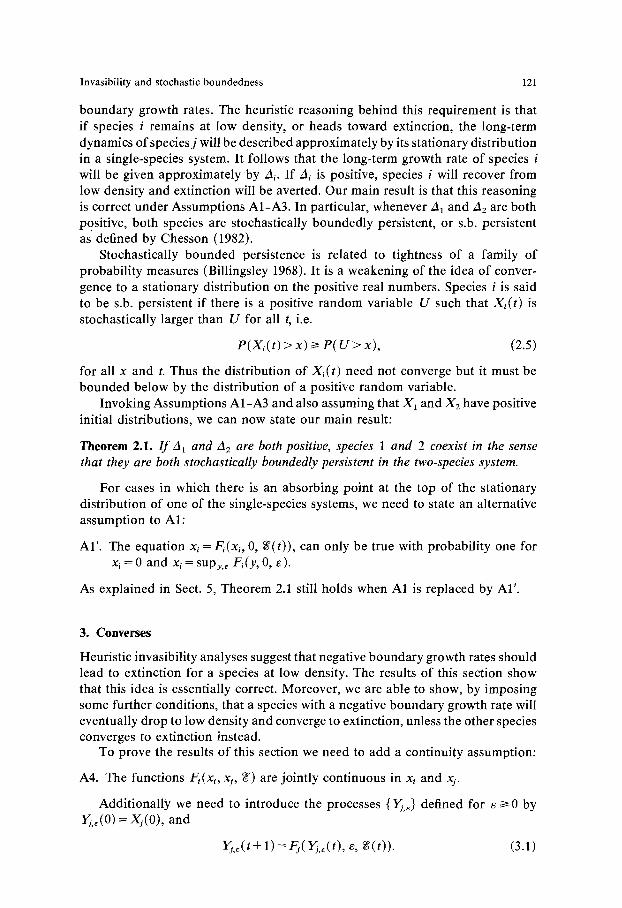
boundary growth rates. The heuristic reasoning behind this requirement is that if species i remains at low density, or heads toward extinction, the long-term dynamics of speciesj will be described approximately by its stationary distribution in a single-species system. It follows that the long-term growth rate of species i will be given approximately by Ai. If A~ is positive, species i will recover from low density and extinction will be averted. Our main result is that this reasoning is correct under Assumptions A1-A3. In particular, whenever dl and A2 are both POsitive, both species are stochastically boundedly persistent, or s.b. persistent as defined by Chesson (1982).

Stochastically bounded persistence is related to tightness of a family of probability measures (Billingsley 1968). It is a weakening of the idea of convergence to a stationary distribution on the positive real numbers. Species i is said to be s.b. persistent if there is a positive random variable U such that X~(t) is stochastically larger than U for all t, i.e.

P(Xi ( t ) > x) >! P( U > x), (2.5)

for all x and t. Thus the distribution of X~(t) need not converge but it must be bounded below by the distribution of a positive random variable.

Invoking Assumptions A1-A3 and also assuming that X1 and X2 have positive initial distributions, we can now state our main result:

Theorem 2.1. I f A 1 and A 2 are both positive, species 1 and 2 coexist in the sense that they are both stochastically boundedly persistent in the two-species system.

For cases in which there is an absorbing point at the top of the stationary distribution of one of the single-species systems, we need to state an alternative assumption to AI:

AI'. The equation xi = F~(xi, 0, ~(t)), can only be true with probability one for xi = 0 and xi = SUpy.~ F/(y, 0, e).

As explained in Sect. 5, Theorem 2.1 still holds when A1 is replaced by AI'.

3. Converses

Heuristic invasibility analyses suggest that negative boundary growth rates should lead to extinction for a species at low density. The results of this section show that this idea is essentially correct. Moreover, we are able to show, by imposing some further conditions, that a species with a negative boundary growth rate will eventually drop to low density and converge to extinction, unless the other species converges to extinction instead.

To prove the results of this section we need to add a continuity assumption:

A4. The functions F~(xi, xj, ~) are jointly continuous in xi and xj.

Additionally we need to introduce the processes { Yj,~} defined for e/> 0 by Y~,~(0) = Xj(0), and

Yj,~(t + 1) = Fj(Yj,~(t), e, ~(t)). (3.1)


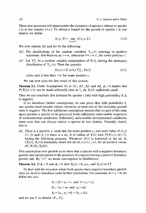
These new processes will approximate the dynamics of species j whenever species i is at low density ( ~ e ) . To obtain a bound for the growth of species i at low density we define

h,(y, ~g)= sup f ( x , y, ~). (3,2) 0~x~e

We now replace A2 and A3 by the following:

A2'. The distributions of the random variables Yj,~(t) converge to positive stationary distributions as t ~ co, whenever 0 ~< e <~ e', for some positive e'.

A3'. Let Y~,~ be a random variable independent of ~( t ) , having the stationary distribution of Yj,~(t). Then the quantity

D,(e) = E In h~( Y*, , ~( t )) (3.3)

exists and is less than +co for some positive e.

We can now state the first result of this section.

Theorem 3.1. Under Assumptions A1 or AI' , A2', A3' and A4, Ai < 0 implies that P(Xi( t) ~ O) can be made arbitrarily close to 1, for Xi(O) sufficiently small.

Thus we can conclude that invasion by species i fails with high probability if A~ is negative.

I f we introduce further assumptions, we can prove that With probability 1, one species must become extinct whenever at least one of the boundary growth rates is negative. The first additional assumption ensures that no part of the state space permits a species to be protected from sufficiently unfavorable sequences of environmental conditions. Sufficiently unfavorable environmental conditions must exist that can always reduce a species to low density. Formally stated, this is:

A5. There is a positive e' such that for every positive e, and each value of (i ,j) ((1,2) and (2, 1)) there is a set A of values of ~( t ) with P(~g( t )~A)>O, having the following property. Whenever ~( t ) is restricted to the set A, (X~(t), Xj( t )) eventually enters the set (0, e] x [e ' , oo), for all positive values of (x~(0), xj(0)).

This assumption now permits us to show that a species with a negative boundary growth rate cannot persist in the presence of a species having a positive boundary growth rate. By " ~ " we mean convergence in distribution.

Theorem 3.2. I f zi i < 0 and Aj > 0 then Xi( t ) ~ O, a.s., and Xj(t)=~ Y~.

To deal with the situation where both species have negative boundary growth rates we need to introduce some further restrictions, For constants m > e > 0, we define the sets

S l = { O < x l < e and 0 < X 2 < E }

S 3 = { x l > m and X z > m }

S 2 = {Xl , X 2 > O} -- ( S 1 k.) 83) ,

and we use F to denote (F1, F2).


A6. There are values of m and e, and a/3 > 0 such that

P{F[x l , x2, ~(t) ] �9 $3} ~ ~P{F(x1, X2, ~(t) �9 $2} ,

for all (Xl, x2) �9 S1.

This restriction means that from $1, the chances of landing next in $2 are at least 1/8 times the chances of landing in $3. A6 is an innocuous assumption for real populations, because it is satisfied whenever there is a finite limit to one species' per-capita growth rate. It is also satisfied if there is an upper bound on the densities that can be reached. In models without such bounds, A6 is essentially equivalent to the existence of the moment generating function of l n f ( 0 , 0, ~( t ) ) for some positive argument. For example, this will be true if the l n f ( 0 , 0, ~( t)) have Gaussian or double exponential distributions. Specifically, let pi.y(x) be the probability density function of l n f ( e - V , O , ~ ( t ) ) . I f l n f ( x l , x 2 , ~ ( t ) ) is sufficiently smooth near xl = x2 = 0, it can be shown that A6 holds whenever

lira sup x -1 In pi, x(x) < ~ ,

i.e. essentially whenever the upper tail of the density converges to 0 exponentially or faster. With the addition of this final assumption we obtain Theorem 3.3:

Theorem 3.3. (b) I f A1, z12 < O, then P(XI(t) ~ 0 or X2(t) -* O) = 1.

Theorems 2.1 and 3.1-3.3 characterize all the behaviors of these processes that are likely to be of interest in practice. Cases where the boundary growth rates may be zero arise occasionally, but as Ellner (1984) has shown for the single-species case, the boundary growth rate by itself is then inadequate to characterize the asymptotic behavior of the process.

Note that it is possible for a process to satisfy Theorem 3.1, but not Theorems 3.2 or 3.3. For example, consider the system obeying the equation

Xi( t + 1) - 2Xi(t)(1 + ~(t){[1 + 9 X j ( t ) ] -1 - 0.1}) (3.4) l+x,(t)

In the case where g~(t) takes values in the interval [8, 9], it is easily seen from Ellner (1984) that the single-species iterations converge to stationary distributions and A3' is satisfied. The remaining assumptions of Theorem 3.1 are easily checked.

For e sufficiently small, the interval [16, 18] is invariant for the single-species processes Yj,~, and hence their stationary distributions are concentrated on this interval. It is now easily checked that the A i are both negative. Theorem 3.1 applies to show that for both X1 and X2 there are initial conditions giving arbitrarily high probabilities of extinction. Theorem 3.3 is not satisfied, however, because the point X1 =)(2 = 1 is left invariant by Eq. (3.4). Since the process never approaches the axes from this point, the boundary growth rates are irrelevant. Stochastic models that have interior invariant points are uncommon and such points are difficult to justify as reasonable possibilities for population dynamics in a stochastic environment. However, interior invariant regions may occur if low-density growth rates are depressed by factors unrelated to competition (Allee effects). Assumption A5 rules out such behavior and seems likely to be satisfied in the majority of applications.


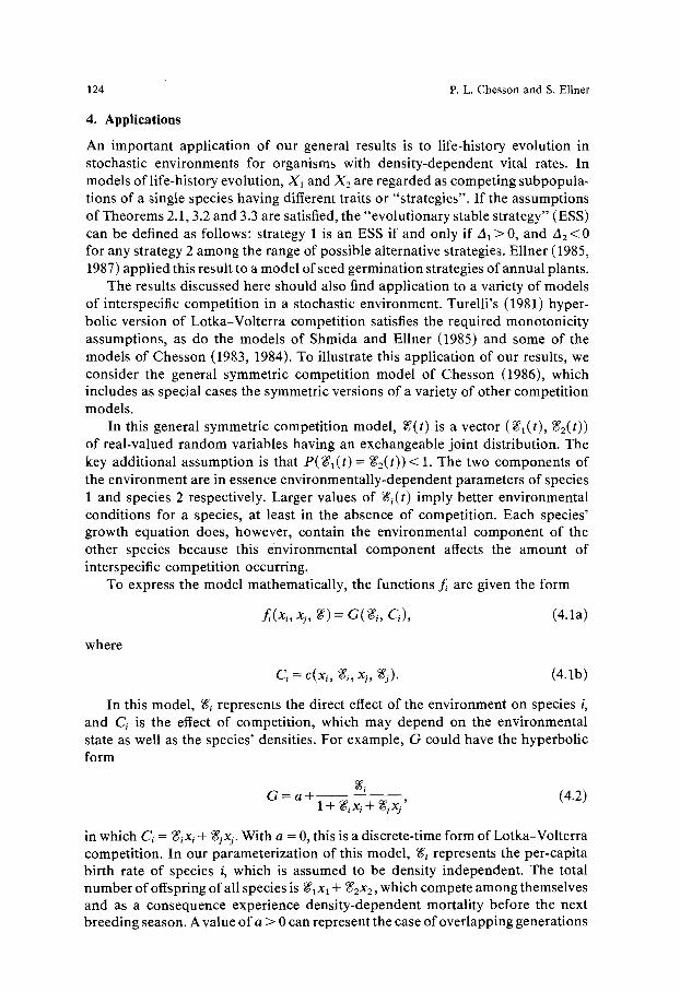
4. Applications

An important application of our general results is to life-history evolution in stochastic environments for organisms with density-dependent vital rates. In models of life-history evolution, X1 and X2 are regarded as competing subpopula- tions of a single species having different traits or "strategies". If the assumptions of Theorems 2.1, 3.2 and 3.3 are satisfied, the "evolutionary stable strategy" (ESS) can be defined as follows: strategy 1 is an ESS if and only if A~>0, and /12<0 for any strategy 2 among the range of possible alternative strategies. Ellner (1985, 1987) applied this result to a model of seed germination strategies of annual plants.

The results discussed here should also find application to a variety of models of interspecific competition in a stochastic environment. Turelli's (1981) hyperbolic version of Lotka-Volterra competition satisfies the required monotonicity assumptions, as do the models of Shmida and Ellner (1985) and some of the models of Chesson (1983, 1984). To illustrate this application of our results, we consider the general symmetric competition model of Chesson (1986), which includes as special cases the symmetric versions of a variety of other competition models.

In this general symmetric competition model, ~( t ) is a vector ( ~ ( t ) , ~2(t)) of real-valued random variables having an exchangeable joint distribution. The key additional assumption is that P ( ~ l ( t ) = ~2( t ) )< 1. The two components of the environment are in essence environmentally-dependent parameters of species 1 and species 2 respectively. Larger values of ~ ( t ) imply better environmental conditions for a species, at least in the absence of competition. Each species' growth equation does, however, contain the environmental component of the other species because this environmental component affects the amount of interspecific competition occurring.

To express the model mathematically, the functions f are given the form

f(x~, xj, ~) = G(~i, C~), (4.1a)

where

C~ = c(x~, ~,, xj, ~j). (4.1b)

In this model, ~i represents the direct effect of the environment on species i, and Ci is the effect of competition, which may depend on the environmental state as well as the species' densities. For example, G could have the hyperbolic form

G = a 4 - - (4.2) 1 + ~ x i + ~jxj'

in which Ci = ~ixi + ~jx~. With a = 0, this is a discrete-time form of Lotka-Volterra competition. In our parameterization of this model, ~i represents the per-capita birth rate of species i, which is assumed to be density independent. The total number of offspring of all species is ~1xl + ~2x2, which compete among themselves and as a consequence experience density-dependent mortality before the next breeding season. A value of a > 0 can represent the case of overlapping generations


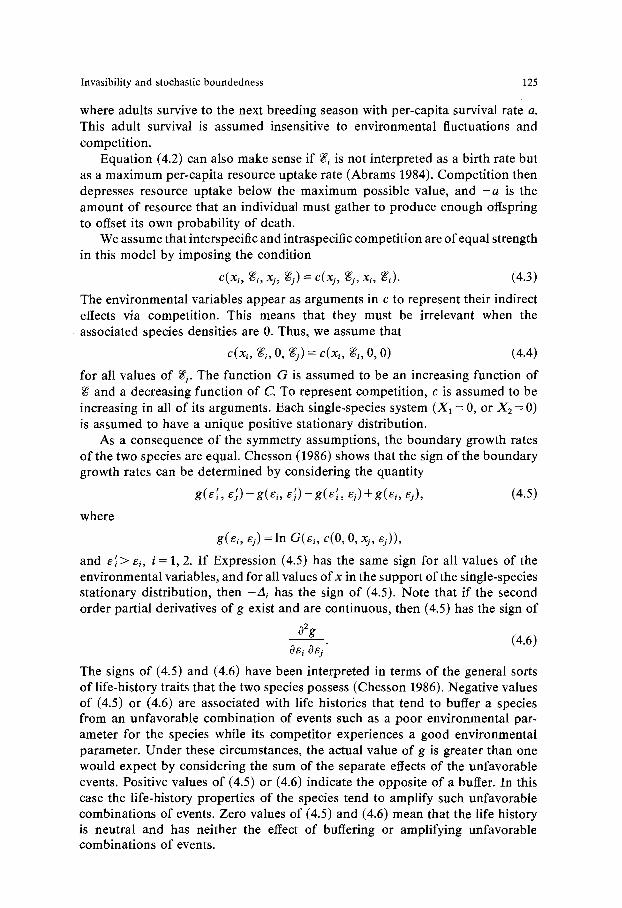
where adults survive to the next breeding season with per-capita survival rate a. This adult survival is assumed insensitive to environmental fluctuations and competition.

Equation (4.2) can also make sense if ~ is not interpreted as a birth rate but as a maximum per-capita resource uptake rate (Abrams 1984). Competition then depresses resource uptake below the maximum possible value, and - a is the amount of resource that an individual must gather to produce enough offspring to offset its own probability of death.

We assume that interspecific and intraspecific competition are of equal strength in this model by imposing the condition

c(xi, ~ , xj, fgj)= c(xj, $j, x~, ~) . (4.3)

The environmental variables appear as arguments in c to represent their indirect effects via competition. This means that they must be irrelevant when the associated species densities are 0. Thus, we assume that

c(x~, ~ , O, ~j) = c(xi, ~;, 0, 0) (4.4)

for all values of ~j. The function G is assumed to be an increasing function of and a decreasing function of C. To represent competition, c is assumed to be

increasing in all of its arguments. Each single-species system (X1 = 0, or X2 = 0) is assumed to have a unique positive stationary distribution.

As a consequence of the symmetry assumptions, the boundary growth rates of the two species are equal. Chesson (1986) shows that the sign of the boundary growth rates can be determined by considering the quantity

g( e~, e;) - g( e,, e;) - g( el, ej) + g( e,, ej), (4.5)

where

g(e~, ej) = In G(e,, c(O, O, xj, ej)),

and e l > e~, i = 1, 2. If Expression (4.5) has the same sign for all values of the environmental variables, and for all values of x in the support of the single-species stationary distribution, then -A~ has the sign of (4.5). Note that if the second order partial derivatives of g exist and are continuous, then (4.5) has the sign of

02g (4.6) 0e; 0ej"

The signs of (4.5) and (4.6) have been interpreted in terms of the general sorts of life-history traits that the two species possess (Chesson 1986). Negative values of (4.5) or (4.6) are associated with life histories that tend to buffer a species from an unfavorable combination of events such as a poor environmental parameter for the species while its competitor experiences a good environmental parameter. Under these circumstances, the actual value of g is greater than one would expect by considering the sum of the separate effects of the unfavorable events. Positive values of (4.5) or (4.6) indicate the opposite of a buffer. In this case the life-history properties of the species tend to amplify such unfavorable combinations of events. Zero values of (4.5) and (4.6) mean that the life history is neutral and has neither the effect of buffering or amplifying unfavorable combinations of events.


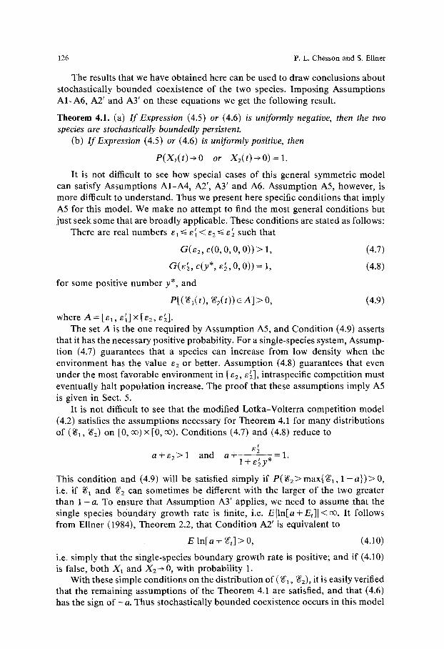
The results that we have obtained here can be used to draw conclusions about stochastically bounded coexistence of the two species. Imposing Assumptions A1-A6, A2' and A3' on these equations we get the following result.

Theorem 4.1. (a) I f Expression (4.5) or (4.6) is uniformly negative, then the two species are stochastically boundedly persistent.

(b) I f Expression (4,5) or (4.6) is uniformly positive, then

P(XI(t)--)O or X2(t ) - )0) - -1 .

It is not difficult to see how special cases of this general symmetric model can satisfy Assumptions A1-A4, A2', A3' and A6. Assumption A5, however, is more difficult to understand. Thus we present here specific conditions that imply A5 for this model. We make no attempt to find the most general conditions but just seek some that are broadly applicable. These conditions are stated as follows:

There are real numbers E 1 ~ E~ • E2~ E2 such that

G(e2, c(0, 0, 0, 0)) > 1, (4.7)

G(e'2, c(y*, eL, 0, 0)) = 1, (4.8)

for some positive number y*, and

P [ ( ~ ( t ) , ~;(t)) c A] > 0, (4.9)

where A = [ e l , e~]x[e2, eL]. The set A is the one required by Assumption A5, and Condition (4.9) asserts

that it has the necessary positive probability. For a single-species system, Assump- tion (4.7) guarantees that a species can increase from low density when the environment has the value e2 or better. Assumption (4.8) guarantees that even under the most favorable environment in [e2, eL], intraspecific competition must eventually halt population increase. The proof that these assumptions imply A5 is given in Sect. 5.

It is not difficult to see that the modified Lotka-Volterra competition model (4.2) satisfies the assumptions necessary for Theorem 4.1 for many distributions of (~1, ~2) on [0, oo) x [0, oo). Conditions (4.7) and (4.8) reduce to

e; a + e 2 > l and a + - - - 1 .

l + e ~ y *

This condition and (4.9) will be satisfied simply if P(~2 > max{ ~1,1 - a}) > 0, i.e. if ~1 and ~2 can sometimes be different with the larger of the two greater than 1 - a. To ensure that Assumption A3' applies, we need to assume that the single species boundary growth rate is finite, i.e. Elln[a+E~]l<oo. It follows from Ellner (1984), Theorem 2.2, that Condition A2' is equivalent to

E ln[a + ~,] > 0, (4.10)

i.e. simply that the single-species boundary growth rate is positive; and if (4.10) is false, both X~ and X2 ~ 0, with probability 1.

With these simple conditions on the distribution of (~1, ~2), it is easily verified that the remaining assumptions of the Theorem 4.1 are satisfied, and that (4.6) has the sign of - a . Thus stochastically bounded coexistence occurs in this model


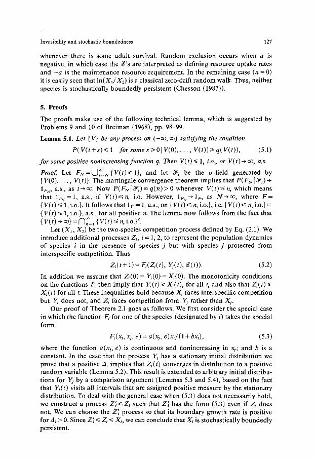
whenever there is some adult survival. Random exclusion occurs when a is negative, in which case the ~'s are interpreted as defining resource uptake rates and - a is the maintenance resource requirement. In the remaining case (a = 0) it is easily seen that ln(X1/X2) is a classical zero-drift random walk. Thus, neither species is stochastically boundedly persistent (Chesson (1987)).

5. Proofs

The proofs make use of the following technical lemma, which is suggested by Problems 9 and 10 of Breiman (1968), pp. 98-99.

Lemma 5.1. Let { V} be any process on ( - ~ , o0) satisfying the condition

P ( V ( t + s ) < - I forsomes>~O[ V(O), . . . , V(t))>-q(V(t)) , (5.1)

for some positive nonincreasing function q. Then V ( t ) <~ 1, i.o., or V( t ) ~ ~ , a.s.

Proof. Let FN=US_N{V( t )<~I} , and let fit be the o--field generated by { V ( 0 ) , . . . , V(t)}. The martingale convergence theorem implies that P(FN[~t) I~N, a.s., as t - ~ . Now P ( F n l ~ ) > - q ( n ) > O whenever V(t)<-n, which means that l p N = l , a.s., if V(t)<-n, i.o. However, 1 F ~ l e , as N ~ , where F = { V(t) ~ 1, i.o.}. It follows that 1 v = 1, a.s., on { V(t) ~< n, i.o.}, i.e. { V(t) ~< n, i.o.} c {V(t) ~ 1, i.o.}, a.s., for all positive n. The lemma now follows from the fact that { V(t) ~ cO} = n~=a { V(t) ~ n, 1.o.} .

Let (X~, X2) be the two-species competition process defined by Eq. (2.1). We introduce additional processes Zi, i = 1, 2, to represent the population dynamics of species i in the presence of species j but with species j protected from interspecific competition. Thus

Zi(t+ 1) -- F~(Zi(t), Yj(t), ~(t)). (5.2)

In addition we assume that Zi(0)= Y/(0)= X~(0). The monotonicity conditions on the functions F~ then imply that Y~(t)/> X~(t), for all t, and also that Z~(t)<~ X~(t) for all t. These inequalities hold because X; faces interspecific competition but Y~ does not, and Zi faces competition from Yj rather than Xj.

Our proof of Theorem 2.1 goes as follows. We first consider the special case in which the function F~ for one of the species (designated by i) takes the special form

F,(x,, xs, e) = a(xj, e)x,/(1 + bxi), (5.3)

where the function a(xs, e) is continuous and nonincreasing in xs; and b is a constant. In the case that the process Yj has a stationary initial distribution we prove that a positive A~ implies that Z~(t) converges in distribution to a positive random variable (Lemma 5.2). This result is extended to arbitrary initial distributions for Yj by a comparison argument (Lemmas 5.3 and 5.4), based on the fact that Yj(t) visits all intervals that are assigned positive measure by the stationary distribution. To deal with the general case when (5.3) does not necessarily hold, we construct a process ZI ~< Zi such that Z~ has the form (5.3) even if Zi does not. We can choose the Z~ process so that its boundary growth rate is positive for/t~ > 0. Since Z~ ~< Z~ ~< X~, we can conclude that X~ is stochastically boundedly persistent.


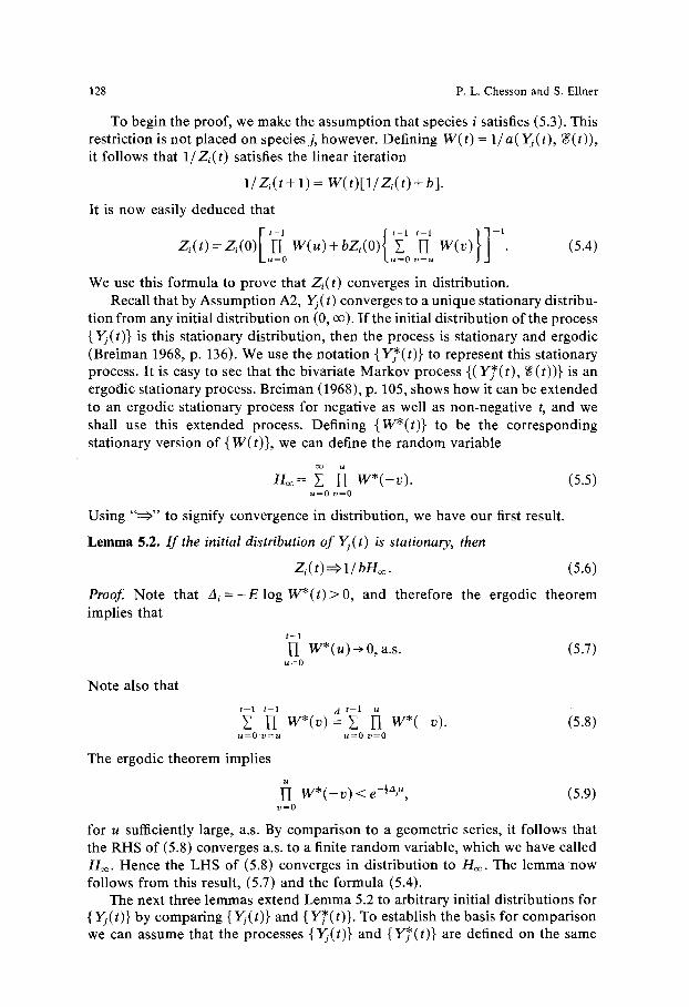
To begin the proof, we make the assumption that species i satisfies (5.3). This restriction is not placed on species j, however. Defining W(t) = 1/a (Yj(t), ~(t)), it follows that 1/Zi(t) satisfies the linear iteration

1/Z~(t + 1) = W(t)[1/Z,(t) + b].

It is now easily deduced that

[iH10 t]1 Z~(t)=Z,(O W(u)+bZ~(O [I W(v (5.4)

We use this formula to prove that Zi(t) converges in distribution. Recall that by Assumption A2, Yj(t) converges to a unique stationary distribu-

tion from any initial distribution on (0, ~) . If the initial distribution of the process { Yj(t)} is this stationary distribution, then the process is stationary and ergodic (Breiman 1968, p. 136). We use the notation { Y*(t)} to represent this stationary process. It is easy to see that the bivariate Markov process {(Y*(t), ~(t))} is an ergodic stationary process. Breiman (1968), p. 105, shows how it can be extended to an ergodic stationary process for negative as well as non-negative t, and we shall use this extended process. Defining {W*(t)} to be the corresponding stationary version of { W(t)}, we can define the random variable

w*(-v). (5.5) u = 0 v = 0

Using " ~ " to signify convergence in distribution, we have our first result.

Lemma 5.2. I f the initial distribution of Yj( t ) is stationary, then

Zi(t)~l/bHo~. (5.6)

Proof. Note that A ~ = - E l o g W * ( t ) > 0 , and therefore the ergodic theorem implies that

Note also that

t--1

l-I W*(u) ~ O, a.s. (5.7) u = 0

t--1 t - - I d t--1 u

I-I w*(v )= Y~ I-I w*( -v ) . (5.8) u = O v = u u = 0 v = 0

The ergodic theorem implies

(I W*(-v) < e - ~ y , (5.9) V = 0

for u sufficiently large, a.s. By comparison to a geometric series, it follows that the RHS of (5.8) converges a.s. to a finite random variable, which we have called Ho~. Hence the LHS of (5.8) converges in distribution to Ho~. The lemma now follows from this result, (5.7) and the formula (5.4).

The next three lemmas extend Lemma 5.2 to arbitrary initial distributions for { Yj(t)} by comparing { Y~(t)} and { Y*(t)}. To establish the basis for comparison we can assume that the processes {Yj(t)} and {Y~(t)} are defined on the same


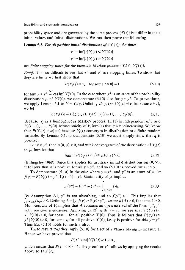
probability space and are governed by the same process { ~(t)} but differ in their initial values and initial distributions. We can then prove the following.

Lemma 5.3. For all positive initial distributions of {Yj(t)} the times

~-- =inf{t [ Yj(t) ~< Y*(0)}

z+ =inf{t [ Yj(t) ~> Y*(0)}

are finite stopping times for the bivariate Markov process { Yj(t), Y*(t)}.

Proof It is not difficult to see that z- and ~'+ are stopping times. To show that they are finite we first show that

P{Yj(t)<~y, forsome t~>0} = 1 (5.10)

def for any y > y* = ess inf Y*(0). In the case where y* is an atom of the probability distribution/X of Y*(0), we demonstrate (5.10) also for y - -y* . To prove these, we apply Lemma 5.1 to V= YJy. Defining D(y, t)= {Yj(s) ~<y, for some s ~ > t}, we let

q(Yj(t))=P{D(y, t)l Yj(t), Y j ( t - 1) . . . . , Yj(0)}. (5.11)

Because Y~ is a homogeneous Markov process, (5.11) is independent of t and Yj ( t - 1 ) , . . . , Yj(0). Monotonicity of Fj implies that q is nonincreasing. We know that P(Yj(t) ~ o0)= 0 because Yj(t) converges in distribution to a finite random variable. By Lemma 5.1, to demonstrate (5.10) we must simply show that q is positive.

Let y > y*, then tz(0, y) > 0, and weak convergence of the distribution of Yj(t) to/X, implies that

liminf P(Yj(t) < y)/>/X(0, y) > 0, (5.12)

(BiIlingsley 1968). Since this applies for arbitrary initial distributions on (0, oo), it follows that q is positive for all y>y*, and so (5.10) is proved for such y.

To demonstrate (5.10) in the case where y =y* , and y* is an atom of/x, let f (y) = P(Yj(t) = Y*I Yj(t - 1) = y). Stationarity of/X implies

/x{y*} =f(y*)/x{y*} + f fd/x. (5.13) J~ y*,~)

By Assumption A1, y* is not absorbing, and so f (y*)< 1. This implies that 5(y* o~)fd/x > 0. Defining A = {y If(Y) > 6, y > y*}, we see/X (A) > 0, for some ~ > 0. Monotonicity of Fj implies that A contains an open interval of the form (y*, y') with positive p~-measure. Applying (5.12) with y =y ' , we see that P(Yj(t)< y'] Yj(0))> 0, for some t, for all positive Y~(0). Thus, it follows that P(Yj(t)<~ Y*I Yj(0))> 0, for some t, for all positive Yj(0), i.e. q is positive for this y =y*. Thus Eq. (5.10) holds for such y also.

These results together imply (5.10) for a set of y values having/x-measure 1. Hence we have proved that

P ( r - < c~[ Y*(0)) = 1, a.s.,

which means that P(z- < 0o) = 1. The proof for r + follows by applying the results above to 1/Yj(t).

130 P. L. Chesson and S. Ellner

The stopping times ~-+ and ~'- are used to construct processes that bound Y~. To use the lemma we note that any stopping time v for { Yj(t), Y*(t)} allows us to define a new process Y* by the relationships

Y*~(t+ 1) = Fj(Y*(t) , ~(t+ v)), (5.14)

and Y*(0)= Y*(0). Since ~(t)} is an i.i.d, process, the strong Markov property implies that the bivariate Markov processes {(Y*(t),~(t+v))} and {(Y*(t), ~(t))} are identically distributed. Since by definition Yj(r-)<~ Y*-(0), and Fj is monotonic, it is easy to see that Yj(t+ ~--)~< Y*-(t) for all nonnegative t. We can use these results to prove a law of large numbers:

Lemma 5.4.

1 l - - 1 a . S .

- ~ l o g W ( u ) - > - - A ~ < O . t u=O

Proof Defining W*-(t)= 1/a(Y*-(t), ~ ( t + ~--)) we see that

w ( t + 7-) ~ w*~-(t) (5.15)

because a(y, ~) is nonincreasing in y and Yj(t+ z-)<~ Y*(t). The strong law of large numbers for log W*-(t) implies that

1 f--1

l imsuP t ~ log W(u+'r-)<<--Ai, a.s. (5.16) u = 0

and hence that

1 t--1

l imsuP t Y~ log W(u)<~-Ai, a.s. (5.17) u = 0

Similarly, consideration of ~'+ implies

t - 1

liminf 1 ~ log W(u) >l-Ai, a.s. (5.18) t u = 0

The lemma follows from (5.17) and (5.18). We are now in a position to prove that Zj(t) converges in distribution for

general initial distributions of Y~(t).

Lemma 5.5. If Yi(0) > 0, then

Proof Define

Zj(t)~l/bH~.

d d

H(c, d) = Y~ I] W(v). (5.19) u = c v = u

and let H*-(c, d) be the corresponding random variable involving W*-(t). It was shown in the proof of Lemma 5.2 that when the initial distribution is stationary, H(O,d)~H~, as d~oo . This applies to H*-(O,d) because any Y* has the stationary initial distribution.


NOW H(z- , t+ z-) <~ H*-(O, t), and since H* (c, d) is independent of ~-, we have

E[f{H('r-, t + T-)}[ z-] ~< Ef{H*~-(O, t)},

for every nondecreasing bounded continuous function f Because z- takes values in a countable set we can now conclude that

limsup E[f(H(,r-, t + z - ) ) [ z - ] ~< Ef(H~), a.s. (5.20)

This inequality can be improved upon by noting that

H ( O , t + z - ) - H ( z - , t + z - ) = W(v) H(0, z - - 1). (5.21) x o = ~ -

Lemma 5.4 now implies that H(0, t+~- ) - H ( z - , t+z- )~O, a.s., as t~co . The properties o f f mean that it is uniformly continuous. Hence (5.20) and (5.21) imply that

limsup E[f(H(O, t+~'-)lr-]<~Ef(Hoo), a.s., (5.22)

from which we conclude

limsup E[f(H(O, t ) ) [ r - ] ~< Ef(H~), a.s. (5.23)

Similarly

liminf E[f(H(O, t ) ) lz +]/> Ef(H~), a.s. (5.24)

The fact that f is bounded means that Fatou's lemma applies to both (5.23) and (5.24). Thus we can integrate over the distributions of the ~-'s to conclude that

lira Ef( H ( O, t ) ) = Ef( H~). (5.25)

Because the class of continuous bounded nondecreasing functions is a convergence determining class, it follows that H(0, t)~Ho~. Applying this result and Lemma 5.4 to expression (5.4) for Z~(t), completes the proof.

The fact that X~(t)>1 Z~(t) now allows us to conclude stochastically bounded persistence for Xg(t) when F~ takes the form (5.3), that is:

Lemma 5.6. I f F~ takes the hyperbolic form (5.3) then

liminf P(X~(t) > x) >~ P(1/bH~> x)

for all positive x.

To prove stochastically bounded persistence for the general case we note that Condition A3 allows the monotone convergence theorem to be applied to di(ri) and so we can conclude that there is a positive r such that

di(r)/> �89 > 0, (5.26)

for some positive r. Given such an r, define

a(y, ~ ) = inf f (x , y, ~) (5.27) O ~ x ~ r


and let F'i be defined by the RHS of (5.3) with b = 1/r. The process Z'~ is defined in terms of F'i identically to the definition of Zi in terms of F~. These two processes have an inequality between them:

Lemma 5.7. Zl( t ) <~ Zi(t) for all t.

Proof. First note that for 0 <~ z <~ r, F'i (z, y, 3) ~< F~ (z, y, 3 ) / ( 1 + bz); while for z > r, we have SUpz F'~(z, y, 3) = ra(y, 3) ~ F/(r, y, 3) <~ Fi(z, y, 3). Thus we conclude that F~(z, y, g') ~ Fg(z, y, 3) for all z, y, 3. The proof is now completed by mathematical induction noting that Z~(0)--Z~(0) and using the fact that Z l ( t ) ~ Z~(t) implies

Zl ( t+ 1) -- F~(Z'~(t), Yj(t), 3(t)) <~ FI(Z~(t), Yj(t), ~( t ) )

<~ F~(Z~(t), Yj(t), ~( t ) ) = Z,( t+ 1).

This result yields the following immediate generalization of Lemma 5.6.

Lemma 5.8. liminf P(Xi (t) > x) >1 P(1/bHoo > x) for all positive x.

This lemma is merely another way of stating Theorem 2.1. To prove Theorem 2.1 for the case in which there is an invariant point at the

top of the range of the single species process, i.e. when Assumption AI' replaces A1, we define x~* = supy,~ F~(y, 0, e). Under AI', the stationary distribution of Yj(t) assigns probability 1 or 0 to x*. In the latter case, the point x* can be removed from the state space, and Assumption A1 can be used. In the former case, we simply define Z~ with Y* substituting for Yj. It is still true that Z'~ ~ X~. Lemma 5.2 then applies to Z'~, and the conclusions of Lemma 5.8 follow immediately.

To prove Theorem 3.1 we must show that the boundary growth rates, the Ai, can be approximated suitably using the stationary distributions of the Y~,~. We begin by showing that the stationary distribution, /~, of Y~ converges to the stationary distribution, ~, of Y~.

Lemma 5.9. As e ~O, I~=#Iz, and Di(e)-> Ai.

Proof The monotonicity assumptions on the F~ imply that

Yj.~,(t) ~ Yj,~(t)-< Y~,0(t), (5.28)

whenever 0 < s < e'. It follows that the sequence {/x,, 0 < s < s'}, where e' is any positive number, is a tight sequence. Moreover, the monotonicity of the sequence implies that it converges weakly as e-~0 to some probability measure /~*. To prove that /z* equals/z, note that the continuity assumptions A4 on the F~ imply that

Ef[Fj(x~, e, ~(t))]--> Ef[F2(x, O, ~(t))] , (5.29)

as e ~ 0, whenever f is a bounded continuous function and {x,} is a positive sequence converging to a positive number x. Defining U~ to be the transition operator of { Y~,~}, this can be restated as (U ~f ) (x , )~ (Uof)(x). Lemma A2 of Chesson (1982) now implies that

f u~f d~ ~ f Uof d~ * (5.30)

lnvasibility and stochastic boundedness 133

for all bounded continuous f. However, since the Ix, are stationary measures, the LHS above equals ~fdix~, which converges to ~fdix*. Thus I Uofdix* =jfdix*, proving that Ix* is the unique stationary measure of Yj, o, i.e. Ix* = IX.

To complete the proof of the lemma we note that the continuity assumptions A4 imply that h~(y, ~) is jointly continuous in e and y. Random variables Y* having the stationary distribution IX~ can be assumed to form a monotone increasing sequence converging everywhere to Yy*,o (Billingsley (1971)). This means that h~(Y* ~(t))J, ho(Y*o, ~(t)). Assumption A3' and the monotone convergence theorem now imply that

D,(e) ~ A, (5.31)

as s$O. Since &<O, assume that z has been chosen so that D~(s)<0. Define the

process {Z~,~} to approximate {X~} near 0 by Z~.~(O)=Xi(O) and Z i ,~ ( t+ l )= Zi,~(t)h~(Yj,~(t), ~( t ) ) .

Lemma 5.10. As too t , Zi.~( t)-~O, a.s.

Proof. Applying Lemma 5.4 with h~(Yj.~(t), ~g(t)) substituted for W ( t )= 1/a(Yj(t), ~(t)), we see that

1 t--1 a,s .

- E log h~(Yj.~(t), g'(t)) , Oz(e)<0 . (5.32) t u=o

Since In Z~,~(t+ 1 ) - l n Zi,~(t)=ln h~(Yj,~(t), ~(t)) , this proves the lemma. On the set At = {X~(0), X i ( 1 ) , . . . , X~(t - 1) ~< e}, it is easily seen that X / u ) >~

Yj, du ) , u = 0 . . . . , t, and X~(u)<~Z~,~(u), u = 0 . . . . , t + l . From Lemma 5.10, it follows that

Xi(t)-~O, a.s., on A ~ - At. (5.33) t = 0

The proof of the theorem thus requires a proof that P(A~)--, 1, as X~(0) ~ 0. To this end we note the following technical lemma.

Lemma 5.11. Let the sequence of random variables { Ut} satisfy a law of large numbers ] t--1 a.s .

- ~ U~ ~ Ix < 0. (5.34) t s=O

Then

) P s p ~ U ,>x ~0, a s x - ~ . s ~ O

Proof The hypothesis of the lemma implies that there is, a.s., a last time that t - - I t - - I

~s~o Us i> O. It follows that sup, ~ 0 Us exists as a finite random variable. The lemma follows immediately.

Note that

[ ] P(A~) = P sup E logf~(X,(u), X~(u), Cg(u)) ~ e - l o g X,(0) u ~ 0

[ ] ~>e sup E logZ, .~(u+l) /Zi .~(u)~e-logX,(O) . (5.35) u ~ O


Lemma 5.11 applies to log Zi,~(t+ 1)/Zi,~(t)= U,. We conclude that P(Aoo)~ 1, as X~(0)-~ 0. This completes the proof of Theorem 3.1.

To prove Theorem 3.2 we make further use of the monotonicity properties of the process (X1, X2). In particular, if (X~, X~) is another competition process obeying the same iterative equation as (X1, X2) but having possibly different initial values, then the following lemma is easily proved.

Lemma 5.12. I f X~(O) <~ XI(O) and Xj(O) >! X~(O) then Xi( t) <~ Xl ( t) and Xj( t) >1 X~(t) for all t.

Theorem 3.1 implies that for every e ' > 0 there are positive numbers e and p such that

P(Ao~] X~(0)= e, Xj(0)= e ' )=p . (5.36)

Using Lemma 5.12 we see that this extends to the statement

P(A~ I X~(O), Xj(0)) ~>p, (5.37)

whenever X~(0) <~ e and Xj(0) ~> e'. This shows that whenever the process enters the set B = (0, e] x [e', m), there is probability at least p that X~(t) --> 0. A straight- forward generalization of Lemma 3.2 of Chesson (1982) now yields the following.

Lemma 5.13. (Xi(t), Xj(t)) ~ B, i.o., implies Xi(t) --> O, a.s.

To see when (Xi(t), Xj( t ) )E B i.o., we introduce the process {V(t)} defined by the equation

V( t) = max{Xi( t)/ e, e'/ Xj( t)}. (5.38)

Note that V(t)~< 1 implies that (X~(t), Xj ( t ) )~ B. The monotonicity properties of (X1, X2) imply the following.

Lemma 5.14. There is a positive nonincreasing function q on (0, ~) such that

P(V( t+s )<~l f o r s o m e s ~ O l V ( O ) , . . . , V ( t ) ) ~ q ( V ( t ) ) . (5.39)

Proof Define

q(v) = P(V(t+s)<~ 1 for some s~OlX~(t) = ev, Xj(t) = e'/v).

Lemma 5.12 and the Markov property of (X1, X2) immediately imply inequality (5.39) and that q is nonincreasing. That q is positive is a simple consequence of Assumption A5.

The particular process { V} defined here satisfies Lemma 5.1. Combining this with Lemma 5.13, we can now conclude:

Lemma 5.15. I f Ai <O , Aj>0, then Xi(t)-->0, a.s. and X ~ ( t ) ~ Yj*. .

Proof From Lemma 5.1 we have a.s. either V(t)<~ 1, i.o. or V( t )~oQ The first possibility implies X i ( t ) ~ O, a.s., by Lemma 5.13. The second possibility implies that

X i ( t ) > e n or X~(t )<e ' /n , (5.40)

for t sufficiently large, for every n. To see that this scenario has probability 0, define


and

w.(t) =7.=, l~:,jr176

As a consequence of (5.40),

P ( V ( t ) --> 0o) ~ E l iminf ( U , ( t ) + W,( t ) ) <. l iminf[EUn(t) + EW,( t )] .

However , the distr ibutions of the Xi(t) are a tight sequence because Xi(t) <~ Y~(t), which converges in distribution. It follows that EU,(t)--> 0 as n--> co, un i formly in t. L e m m a 5.7 implies that 1 /Xj (t) is tight also, which means that also E Wn (t) --> 0 uni formly in t. Thus P ( V ( t ) --> co) = 0, and we can conclude that X~(t) --> O, a.s.

To show that Xj( t ) converges in distribution, we note that Xj( t ) ~< Yj(t). The distr ibution of Yj(t) converges to ~, the unique s ta t ionary distribution. This means that the distr ibutions of Xj (t) are tight and any limit v of these distr ibutions obeys the inequali ty v(x, co)<~ t.e(x, co), for all x. To prove the reverse inequali ty we define Y~,r(t), for t ~ > T by letting Y~.T(T)= Xj(T) , and

Y~,T(t+ 1) = Fj(Y~,T(t), e, $(t)) .

Assumpt ion A2' implies that the distr ibutions of Y~,r(t) converge, as t--> co, to the measures /z~ , which in turn converge to ~ as e-> 0 ( L e m m a 5.9).

Since X~(t)-->0, a.s., there is a last t ime ~- for which X~(~ ' )>e. I f T > r , Y~,r( t) < Xj( t). Thus

P(Y~,T( t )~Xj ( t ) , for all t ~ > T)--> 1

as T->co. In part icular , for T sufficiently large,

P(Y~,r(t) <~ Xj( t) ) >i 1 - 6,

for t ~> T, given arbi t rary 6. It follows that

P [ x < Y~,T(t)]<~P[x<Xj(t)]+3,

for all x. The limiting distr ibutions of these r a n d o m variables must satisfy this same inequality, and since 6 is arbitrary, this means that

~ ( x , co) < ,,(x, co).

N o w letting e ~ 0, and recall ing that v(x, co) <~ tz(x, co), we see that v = ~. Hence the distr ibutions of Xj( t ) converge to /z , i.e. X j ( t ) ~ Y*.

To prove Theorem 3.3 we begin with the following:

Lemma 5.16. Let W be the e v e n t {Xl(t)-->0 or X2(t)->0}. I f Al<O and A 2 < 0 , then both of the events

{max(Xl ( t ) , X2(t)) < 1/n, i.o.}

and

{min(Xl( t ) , X2(t)) > n, i.o.}

occur a.s. on W c, for every n > 1.


Proof Let V1 and 112 be defined by (5.38) with i = 1 and 2, respectively. As in Lemma 5.15 we have that V,(t)~oo and V2(t)~oo, a.s. on W c. This implies that a.s. on W ~, for t sufficiently large

Xl(t) and X2( t )< 1/n, or X,(t) and X2( t )> n. (5.41)

On W c, l i m s u p X , ( t ) > 0 and by comparison with Y, as in Lemma 5.15, liminf X, (t) < oo, a.s. Thus W c = W ~ c~ {limsup X1 > 0, liminf X1 < co}. Let

Lk = W ~ ~ {liminf X, > 1/k, limsup X, < k}.

We have L k c Lk+l c �9 �9 .W ~ and W ~ = l im Lk. For k > n, on Lk, X~> 1/k i.o. By (5.41), with k substituted for n, X1 and X2 are both > k and hence >n , i.o., a.s. on Lk. Symmetrically, X~ and X2 are both <l/n, i.o., a,s. on Lk. Letting k ~ o o proves the lemma.

To complete the proof of Theorem 3.3, we now use A6 to show that P( W ~) = 0. Let X = (X1, X2) and define the events

A, = { X ( t - 1) �9 s , , x ( t) �9 s~}

and

B, = { X ( t - 1) �9 S~, X ( t ) �9 $2}.

Lemma 5.16, plus (5.41) show that W c c {A, i.o.}, a.s. By the extended Borel- Cantelli Lemma,

{e, i.o.} = { ft=x P[A,+ilX(t),X(t-1),...,X(O)]=oo},a.s.

By the Markov property,

P[At+aIX(t),..., X(O)] = P[X(t+ l) �9 S3[X(t)]l{x(,)es,} ~P[X(t + 1) �9 S2[X( t)]llx(oes,}

= ~P[B,+, IX(t) , . . . , X(O)].

Hence

{A, i.o.}c {,~l P[Bt+l[X(t),...,X(O)]=~176 = {B, i.o.},

which means that WCc {B, i.o.}, a.s. Choosing n appropriately in (5.41) shows that W c c { B t finitely often}, a.s., and hence that P( W e) = 0. This completes the proof of Theorem 3.3.

To show that the competit ion model in Sect. 4 satisfies the necessary assumptions of Theorem 3.2 we must show that Assumption A5 is implied by Assumptions (4.7), (4.8) and (4.9).

Note first of all that if (~i, ~fj) �9 A and xi, xj are confined to a bounded domain (xi, xj <~ K <oo), then we can conclude, using the continuity and monotonicity of G, and equality of Ci and Cj, that

G ( ~ . C,) < p, (5.42)

o(~j, G) where p is a constant less than 1.


If (g'~(t), ~ ( t ) ) is fixed at (e l , eL), then the single-species process Yj(t) must converge to a finite nonrandom value y'<~y*. If instead we have simply (~(t) , ~j(t))cA, then we clearly have limsup Yj(t)<-y '. Now Xj(t) ~ < Yj(t) and so it follows that Xj(t) is bounded less than infinity. Since the LHS of (5.42) cannot be more than 1 for ( ~ ( t ) , g'j (t)) e A, we can conclude that X~(t) is bounded less than oe also. The boundedness of Xj(r implies that

G( ~j(u), C:(u)) < p-,/2 (5.43) u=0

for t sufficiently large, because the RHS converges to infinity. Combining this with inequality (5.42) we conclude

G(g'~(u), C~(u))<p '/2 (5.44) u = O

for t sufficiently large. It follows that Xi(t)-->O, as t-~oe. As a consequence of this, continuity of G and Assumption (4.7), there is an e' such that

G(~j(u), c(xj, ~j(u), Xg(u), g~,(u)) > 1 (5.45)

whenever xj < 2 e ' and u is sufficiently large. It follows that (X~(t), Xj(t)) eventually enters the set (0, e] x [e', co). Hence Assumption A5 is satisfied.

Acknowledgements. We are grateful for several helpful comments of anonymous reviewers. P. Chesson was supported in part by NSF grant BSR-8615028, and S. Ellner was supported in part by a Sir Charles Clore postdoctoral fellowship at the Weizmann Institute of Science.

References

Abrams, P.: Variability in resource consumption rates and the coexistence of competing species. Theor. Popul. BioE 25, 106-124 (1984)

Billingsley, P.: Convergence of probability measures. New York: Wiley 1968 Billingsley, P.: Weak convergence of measures: applications in probability. CBMS-NSF Regional

Conference Series in Applied Mathematics 5. Society for Industrial and Applied Mathematics, Philadelphia, Pennsylvania (1971)

Breiman, L.: Probability. Menlo Park: Addison-Wesley 1968 Chesson, P. L.: Predator-prey theory and variability. Annu. Rev. Ecol. Syst. 9, 323-347 (1978) Chesson, P. L.: The stabilizing effect of a random environment. J. Math. Biol. 15, 1-36 (1982) Chesson, P. L.: Coexistence of competitors in a stochastic environment: the storage effect. In:

Freedman, H. I., Strobeck, C.: (eds.) Population biology (Lect. Notes Biomath., vol. 52, pp. 188-198) Berlin Heidelberg New York Tokyo: Springer 1983

Chesson, P. L.: The storage effect in stochastic population models. In: Levin, S. A., Hallam, T. G.: (eds.) Mathematical ecology: Trieste Proceedings (Lect. Notes Biomath., vol. 54, pp. 76-89) Berlin Heidelberg New York Tokyo: Springer 1984

Chesson, P. L.: Environmental variation and the coexistence species. In: Case, T., Diamond, J.: (eds.) Community Ecology, pp. 240-256. New York: Harper and Row 1986

Chesson, P. L.: Interactions between environment and competition: how fluctuations mediate coexistence and competitive exclusion. In: Hastings, A.: (ed.) Community ecology (Lect. Notes Biomath., vol. 77) Berlin Heidelberg New York Tokyo: Springer: 1988

Connell, J. H., Sousa, W. P.: On the evidence needed to judge ecological stability or persistence. Am. Nat. 121, 789-824 (1983)


Ellner, S. P.: Asymptotic behavior of some stochastic difference equation population models. J. Math. Biol. 19, 169-200 (1984)

Ellner, S.: ESS germination strategies in randomly varying environments. I. Logistic-type models. Theor. Popul. Biol. 28, 50-79 (1985)

Ellner, S.: ESS germination strategies in randomly varying environments. II. Reciprocal-yield laws. Theor. Popul. Biol. 28, 80-116 (1985)

Ellner, S.: Alternate plant life history strategies and coexistence in randomly varying environments. Vegetatio 69, 199-208 (1987)

Grubb, P. J.: The maintenance of species richness in plant communities: the regeneration niche. Biol. Rev. 52, 107-145 (1977)

May, R. M.: On the theory of niche overlap. Theor. Popul. Biol. 5, 297-332 (1974) May, R. M. (ed.): Theoretical ecology: principles and .applications, 2nd edn. Boston: Blackwell 1981 Murdoch, W. W,, Cbesson, J., Chesson, P. L.: Biological control in theory and practice. Am. Nat.

125, 344-366 (1985) Norman, F.: An ergodic theorem for evolution in a random environment. J. Appl. Probab. 12, 661-672

(1976) Prout, T.: The delayed effect on fertility of preadult competition: two-species population dynamics.

Am. Nat. 127, 809-818 (1986) Prout, T., McChesney, F.: Competition among immatures affects their adult fertility: population

dynamics. Am. Nat. 126, 521-558 (1985) Sale, P. F.: Maintenance of high diversity in coral reef fish communities. Am. Nat. 111,337-359 (1977) Schaffer, W., Ellner, S., Kot, M.: The effects of noise~on some dynamical models in ecology. J. Math.

Biol. 24, 479-524 (1986) Schaffer, W. M., Kot, M.: Chaos in ecological systems: the coals that Newcastle forgot. Trends Ecol.

Evol. 1, 58-63 (1986) Shmida, A., Ellner, S.: Coexistence of plant species with similar niches. Vegetatio 58, 29-55 (1985) Slatkin, M.: The dynamics of a population in a Markovian environment. Ecology 59, 249-256 (1978) Strong, D. R.: Density vagueness: abiding the variance in the dynamics of real populations. In:

Diamond, J., Case, T. (eds.) Community ecology, pp. 257-268. New York: Harper and Row 1986 Tanner, J. T.: The stability and intrinsic growth rates of prey and predator populations. Ecology 56,

855-867 (1975) Turelli, M.: Random environments and stochastic calculus. Theor. Popul. Biol. 13, 140-178 (1977) Turelli, M.: Does environmental variability limit niche overlap? Proc. Natl. Acad. Sci. USA 75,

5085-5089 (1978) Turelli, M.: Niche overlap and invasion of competitors in random environments. II. The effects of

demographic stochasticity. In: Jager et al.: (eds.) Biological growth and spread, mathematical theories and applications, pp. 119-129 (1980)

Turelli, M.: Niche overlap and invasion of competitors in random environments I. Models without demographic stochasticity. Theor. PopuL Biol. 20, 1-56 (1981)

Turelli, M., Gillespie, J. H.: Conditions for the existence of stationary densities for some two dimensional diffusion processes with applications in population biology. Theor. Popul. Biol. 17, 167-189 (1980)

Underwood, A. J., Denley, E. L.: Paradigms, explanations, and generalizations in models for the structure of intertidal communities on rocky shores. In: Strong, D. R. Jr., Simberloff, D., Abele, L. G., Thistle, A. B.: (eds.) Ecological communities: conceptial issues and the evidence, pp. 151-180. Princeton: Princeton University Press 1984

Received September 23, 1987/Revised September 9, 1988

Documents

of J. Math. Biol. (1989) 27:117-138 Biologyeebweb.arizona.edu/Faculty/chesson/Peter/Reprints/1989_Invasibility... · J. Math. Biol. (1989) 27:117-138 ,Journal of Mathematical Biology