Embed Size (px)
Citation preview
Of Gluons and Gravitons:Exploring Color-Kinematics Duality
Dissertation
zur Erlangung des Doktorgrades
des Department Physik
der Universitat Hamburg
vorgelegt von
Reinke Sven Isermann
aus Gottingen
Hamburg2013
Gutachter der Dissertation: Jun.-Prof. Dr. Rutger H. Boels
Prof. Dr. Bernd Kniehl
Gutachter der Disputation: Jun.-Prof. Dr. Rutger H. Boels
Prof. Dr. Jan Louis
Datum der Disputation: 14. Juni 2013
Vorsitzender des Prufungsausschusses: Prof. Dr. Caren Hagner
Vorsitzender des Promotionsausschusses: Prof. Dr. Peter Hauschildt
Dekan der Fakultat fur Mathematik,
Informatik und Naturwissenschaften: Prof. Dr. Heinrich Graener

Hey Jude, don’t make it bad.Take a sad song and make it better.
– Hey Jude, The Beatles
In loving memory of my mom.
Abstract
In this thesis color-kinematics duality will be investigated. This duality is a statement aboutthe kinematical dependence of a scattering amplitude in Yang-Mills gauge theories obeyinggroup theoretical relations similar to that of the color gauge group. The major consequenceof this duality is that gravity amplitudes can be related to a certain double copy of gaugetheory amplitudes. The main focus of this thesis will be on exploring the foundations ofcolor-kinematics duality and its consequences. It will be shown how color-kinematics dualitycan be made manifest at the one-loop level for rational amplitudes. A Lagrangian-basedargument will be given for the validity of the double copy construction for these amplitudesincluding explicit examples at four points. Secondly, it will be studied how color-kinematicsduality can be used to improve powercounting in gravity theories. To this end the dualitywill be reformulated in terms of linear maps. It will be shown as an example how this canbe used to derive the large BCFW shift behavior of a gravity integrand constructed throughthe duality to any loop order up to subtleties inherent to the duality that will be addressed.As will become clear the duality implies massive cancellations with respect to the usualpowercounting of Feynman graphs indicating that gravity theories are much better behavedthan naıvely expected. As another example the linear map approach will be used to investigatethe question of UV-finiteness of N = 8 supergravity and it will be seen that the amount ofcancellations depends on the exact implementation of the duality at loop level. Lastly, color-kinematics duality will be considered from a Feynman-graph perspective reproducing some ofthe results of the earlier chapters thus giving non-trivial evidence for the duality at the looplevel from a different perspective.

Zusammenfassung
Der Gegenstand dieser Arbeit ist die Farbkinematische Dualitat. Diese Dualitat besagt, dassdie kinematische Abhangigkeit einer Yang-Mills-Streuamplitude ahnlichen gruppentheore-tischen Relationen genugt wie die Farbladung. Aufgrund dieser Dualitat ist es moglichGraviton-Steuamplituden als eine bestimmte Art von Verdoppelung, auch ”Doppelkopie”genannt, einer Eichtheorie-Amplitude aufzufassen. Der Schwerpunkt dieser Arbeit liegt aufdem Erkunden des theoretischen Fundaments dieser Dualitat und ihrer Konsequenzen. Eswird gezeigt werden, wie die Farbkinematische Dualitat auf Ein-Schleifen-Niveau am Beispielvon rationalen Streuamplituden manifest gemacht werden kann. Die Gultigkeit der Doppelko-pie-Konstruktion fur dieses Beispiel wird anhand der Lagrange-Dichte diskutiert und explizite4-Punkt-Beispiele gezeigt. Desweiteren wird untersucht, wie die Farbkinematische Dualitatdie Abschatzung des oberflachlichen Divergenzgrades in Gravitationstheorien verbessern kann.Hierzu wird die Dualitat als lineare Abbildung aufgefasst. Zur Veranschaulichung dieserHerangehensweise wird zu beliebiger Schleifenordnung das Verhalten von Doppelkopiekons-truierten Gravitations-Integranden fur große BCFW-Verschiebungen hergeleitet. Auf dabeiauftretende Subtilitaten, die der Dualitat zugrunde liegen, wird eingegangen. Wie verdeut-licht wird, impliziert die Dualitat massive Kanzellierungen im Bezug auf den oberflachlichenDivergenzgrad den man fur gewohnlich durch die Abschatzung von Feynman-Diagrammenerhalt, sodass deutlich wird, dass Gravtiationstheorien sich viel besser verhalten als naiver-weise angenommen. Als weiteres Beispiel fur die Nutzlichkeit des Auffassens der Dualitatals lineare Abbildung wird das Auftreten von UV Divergenzen in N = 8 Supergravitationuntersucht. Es wird gezeigt, dass die prazise Implementierung der Dualitat Einfluss auf dieAbschatzung des Divergenzgrades hat. Schließlich wird Farbkinematische-Dualitat direkt mitHilfe von Feynman-Diagrammen untersucht und ausgewahlte Ergebnisse aus den vorherge-henden Kapiteln reproduziert. Diese komplementare Betrachtungsweise bietet nicht-trivialeHinweise fur die Gultigkeit der Dualitat auf Schleifen-Niveau.
Acknowledgment / Danksagung
First and foremost, I would like to express my deep gratitude to my thesis advisor Junior-Professor Rutger Boels who has given me the opportunity to work in one of the most dynamicresearch areas of modern theoretical physics. I am very thankful for his enthusiastic guidance,support, and academical as well as professional advice throughout the past three years. I verymuch enjoyed working with him and hope there will be nontrivial interactions in the future.I am also thankful to Professor Bernd Kniehl and Professor Jan Louis for acting as refereesin my dissertation and disputation, respectively. Moreover, I thank the German ScienceFoundation (DFG) for supporting this work within the Collaborative Research Center 676“Particles, Strings and the Early Universe”.
A big thank you goes out to Ricardo Monteiro and Donal O’Connell for a very exciting andfruitful collaboration; parts of which this thesis is based on. I would like to thank the Niels-Bohr-Institute in Copenhagen for a very pleasant stay and the opportunity to present mywork. Likewise, I am thankful to the physics department in Swansea, in particular DaveDunbar, Warren Perkins, and Sam Alston for a seminar invitation and the hospitable atmo-sphere during my stay.
I am very happy to have met and worked together with many wonderful people in Ham-burg. I would like to thank my office mates Manuel Hohmann, Christoph Horst, MarkusRummel, Martin Schasny, Luca Tripodi, and Lucila Zarate and my fellow amplitudeologistsTobias Hansen, Martin Sprenger, and in particular Gang Yang for many fun and illuminatingdiscussions.
Schließlich bin ich meiner Familie zu allertiefstem Dank verpflichtet: meinem Vater Reinholdfur seine kontinuierliche und selbstlose materielle und immaterielle Unterstutzung wahrendder ganzen Jahre; meiner Frau Katja fur ihre Liebe, Geduld und Ruckendeckung; meinemSohn Julius dafur, dass er mich erdet und die Dinge in Relation setzt.
Thank you.
This thesis is based on the following publications
• R. H. Boels, R. S. Isermann, R. Monteiro, D. O’Connell, Colour-Kinematics Dualityfor One-Loop Rational Amplitudes, arXiv:1301.4165 [hep-th], accepted for publicationin JHEP
• R. H. Boels, R. S. Isermann, On powercounting in perturbative quantum gravity theoriesthrough color-kinematic duality, arXiv:1212.3473 [hep-th], submitted for publication toJHEP
• R. H. Boels, R. S. Isermann, Yang-Mills amplitude relations at loop level from non-adjacent BCFW shifts, arXiv:1110.4462 [hep-th], JHEP 1203 (2012) 051
• R. H. Boels, R. S. Isermann, New relations for scattering amplitudes in Yang-Millstheory at loop level, arXiv:1109.5888 [hep-th], Phys.Rev. D85 (2012) 021701
Contents
1 Introduction: The search for simplicity 1
2 Review of concepts 9
2.1 Organization of gauge theory amplitudes and amplitude relations . . . . . . . 9
2.2 Color-kinematics duality . . . . . . . . . . . . . . . . . . . . . . . . . . . . . . 13
2.3 BCFW shifts and on-shell recursion . . . . . . . . . . . . . . . . . . . . . . . 19
2.4 Generalized inverses . . . . . . . . . . . . . . . . . . . . . . . . . . . . . . . . 23
3 Color-kinematics duality for one-loop rational amplitudes 27
3.1 Manifestly color-dual integrands at one loop . . . . . . . . . . . . . . . . . . . 27
3.2 Examples . . . . . . . . . . . . . . . . . . . . . . . . . . . . . . . . . . . . . . 29
3.2.1 One-loop all-plus amplitude . . . . . . . . . . . . . . . . . . . . . . . . 30
3.2.2 One-loop one-minus amplitude . . . . . . . . . . . . . . . . . . . . . . 34
4 Color-kinematics duality as a linear map 37
4.1 BCFW shifts of gravity tree amplitudes from gauge theory . . . . . . . . . . . 37
4.1.1 Rephrasing color-kinematics duality as linear algebra . . . . . . . . . . 40
4.1.2 BCFW shifts of gravity amplitudes constructed by double copy . . . . 42
4.1.3 Improved shift behavior as a consequence of color-kinematics . . . . . 45
4.1.4 One-loop Yang-Mills relations as a consequence of color-kinematics . . 47
4.2 BCFW shifts of gravity integrands from gauge theory . . . . . . . . . . . . . 48
4.2.1 BCFW shifts of kinematic numerators using generalized inverses . . . 49
4.2.2 BCFW shifts of gravity integrands constructed by double copy . . . . 52
4.3 Estimates on UV behavior from color-kinematics duality . . . . . . . . . . . . 53
viii
5 Towards an off-shell understanding of color-kinematics duality 59
5.1 Non-adjacent BCFW shifts for integrands . . . . . . . . . . . . . . . . . . . . 59
5.1.1 Gluonic contributions . . . . . . . . . . . . . . . . . . . . . . . . . . . 59
5.1.2 Minimally coupled scalar contributions . . . . . . . . . . . . . . . . . . 63
5.1.3 Minimally coupled fermion contributions . . . . . . . . . . . . . . . . . 65
5.1.4 Scalar potential and Yukawa terms . . . . . . . . . . . . . . . . . . . . 67
5.2 Numerator scaling off-shell . . . . . . . . . . . . . . . . . . . . . . . . . . . . . 68
5.2.1 Comparison to BCFW shifts directly via Feynman graphs . . . . . . . 69
5.2.2 BCFW shifts versus color-kinematic duality . . . . . . . . . . . . . . . 70
6 Summary and Outlook 73
Appendix A Spinor-helicity formalism 77
Appendix B Color-ordered Feynman rules 79
Appendix C Feynman graphs used in chapter 5 80
Bibliography 85
ix

x
1. Introduction: The search for simplicity
The study of scattering processes has always been a key tool in almost all branches of physics.
From why the sky is blue, via the properties of crystals, to the structure of atoms and even
beyond: scattering experiments have often guided the way in the quest to understand the
physical laws governing our world.
For the past 70 years the most prominent scattering experiments have been conducted in
high-energy physics, i.e. the study of fundamental particles and their interactions. Theoretical
predictions and experimental results have been complementing each other wonderfully – often
resulting in Nobel Prizes as a nice side effect. For instance the antiproton, predicted by Dirac
in 1933, was experimentally confirmed at the Bevatron at Berkeley in 1955. Experimental
evidence for gluons, theoretically described by Yang and Mills in 1954, was found at the
particle accelerators at DESY in the 1970s. The most recent example of this success story
is the discovery of the Higgs particle in July 2012 at the Large Hadron Collider (LHC) at
CERN, Geneva, almost 50 years after its theoretical prediction in the 1960s.
At the very heart of the theoretical description of particle physics lies the Standard Model
[1–6]. Firmly based on gauge symmetries, this quantum field theory describes how elementary
particles like quarks and leptons interact through three of the four fundamental forces: the
strong, the weak, and the electromagnetic force. The electromagnetic force, with the photon
as its gauge boson, is the fundamental force we are most used to as it describes basically all
everyday phenomena with the exception of gravity. The weak interaction is responsible for
particle decay and neutrino interactions with the Z and W bosons the messenger particles.
The strong force is, as the name suggests, the strongest of the fundamental forces. It binds
protons and neutrons inside nuclei and it describes the interactions between their constituents,
i.e. quarks. The strong force is mediated by gluons. Within the Standard Model, weak and
electromagnetic interactions are described in a unified way in terms of electroweak theory,
the strong interaction through quantum chromodynamics (QCD).
However, as of this writing it is not known how to incorporate gravity into the Standard
Model since there is no known consistent quantum field theory of gravity. The main problem is
that quantizing general relativity will lead to predictions for graviton scattering plagued by UV
divergences. Based on powercounting arguments, it is believed that these divergences cannot
be cured using renormalization techniques because gravity is endowed with a dimensionful
coupling constant. In addition, the Standard Model does not account for certain observations
from cosmology like for instance the abundance of cold dark matter in the universe. Hence
the Standard Model itself can never be a complete theory of particle physics. Despite its
shortcomings it has been a tremendous success nonetheless with many of its predictions like
e.g. the mass of the W or Z bosons confirmed experimentally to a high precision. For more
details regarding the current status of the Standard Model, see [7] and references therein.
1
Ht
g
g
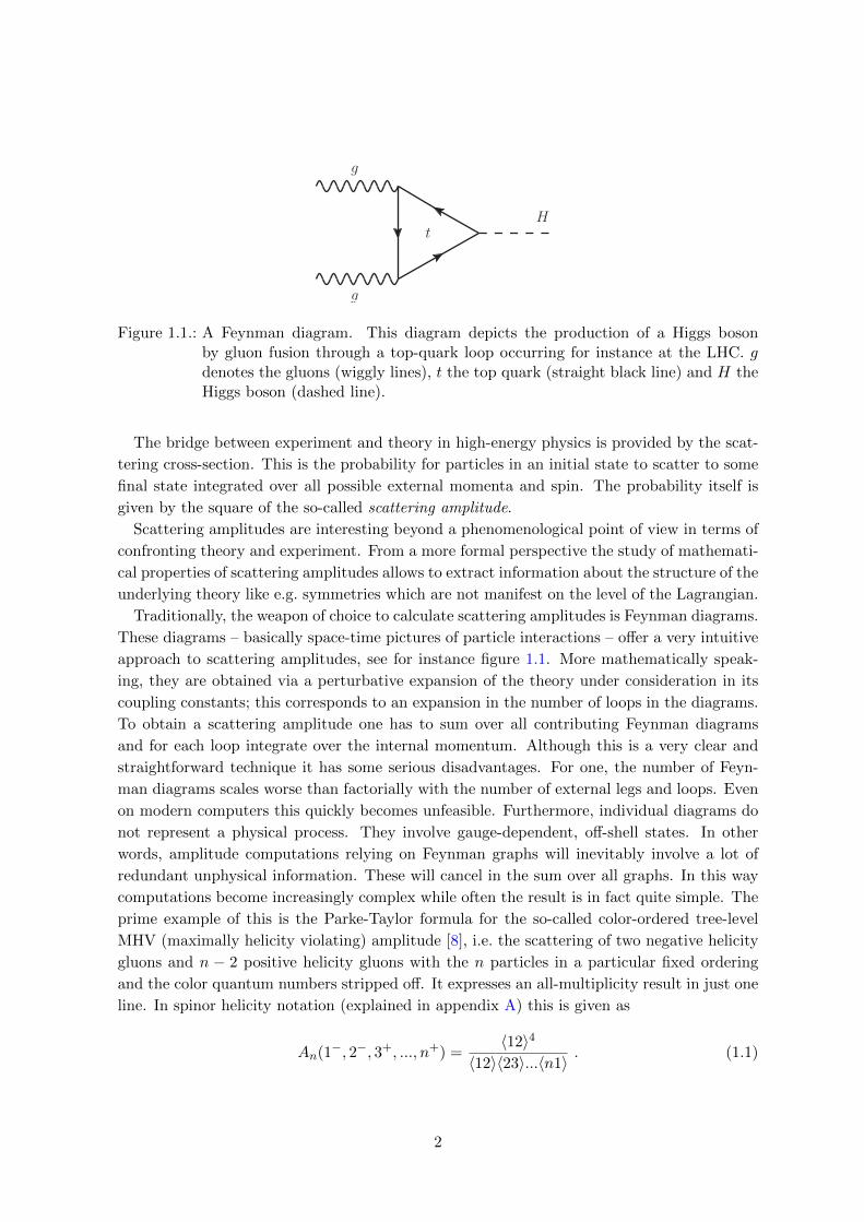
Figure 1.1.: A Feynman diagram. This diagram depicts the production of a Higgs bosonby gluon fusion through a top-quark loop occurring for instance at the LHC. gdenotes the gluons (wiggly lines), t the top quark (straight black line) and H theHiggs boson (dashed line).
The bridge between experiment and theory in high-energy physics is provided by the scat-
tering cross-section. This is the probability for particles in an initial state to scatter to some
final state integrated over all possible external momenta and spin. The probability itself is
given by the square of the so-called scattering amplitude.
Scattering amplitudes are interesting beyond a phenomenological point of view in terms of
confronting theory and experiment. From a more formal perspective the study of mathemati-
cal properties of scattering amplitudes allows to extract information about the structure of the
underlying theory like e.g. symmetries which are not manifest on the level of the Lagrangian.
Traditionally, the weapon of choice to calculate scattering amplitudes is Feynman diagrams.
These diagrams – basically space-time pictures of particle interactions – offer a very intuitive
approach to scattering amplitudes, see for instance figure 1.1. More mathematically speak-
ing, they are obtained via a perturbative expansion of the theory under consideration in its
coupling constants; this corresponds to an expansion in the number of loops in the diagrams.
To obtain a scattering amplitude one has to sum over all contributing Feynman diagrams
and for each loop integrate over the internal momentum. Although this is a very clear and
straightforward technique it has some serious disadvantages. For one, the number of Feyn-
man diagrams scales worse than factorially with the number of external legs and loops. Even
on modern computers this quickly becomes unfeasible. Furthermore, individual diagrams do
not represent a physical process. They involve gauge-dependent, off-shell states. In other
words, amplitude computations relying on Feynman graphs will inevitably involve a lot of
redundant unphysical information. These will cancel in the sum over all graphs. In this way
computations become increasingly complex while often the result is in fact quite simple. The
prime example of this is the Parke-Taylor formula for the so-called color-ordered tree-level
MHV (maximally helicity violating) amplitude [8], i.e. the scattering of two negative helicity
gluons and n − 2 positive helicity gluons with the n particles in a particular fixed ordering
and the color quantum numbers stripped off. It expresses an all-multiplicity result in just one
line. In spinor helicity notation (explained in appendix A) this is given as
An(1−, 2−, 3+, ..., n+) =〈12〉4
〈12〉〈23〉...〈n1〉 . (1.1)
2
Whenever such unexpected cancellations appear, a symmetry not manifest in the calculation
is expected to be at work. All of the above indicates that, while Feynman diagrams are a neat,
intuitive tool for particle physics, they are not the most efficient way to do computations. This
has an even more fundamental, more severe meaning: it shows that we do not understand
Yang-Mills gauge theory as well as we would like to. Surprisingly, it seems to be much simpler
than our understanding allowed us to see.
The same statement holds true for gravity theories. Also graviton scattering amplitudes
show unexpected cancellations. ’t Hooft and Veltman could for instance show by explicit
computations in the 1970s that an expected one-loop divergence for pure gravity amplitudes
is absent [9]. In this way, quite similar to gauge theories, also gravity theories appear to be
much simpler than their corresponding Feynman diagrams lead us to think.
In fact, gauge and gravity scattering amplitudes are very intimately related. At weak
coupling, gravity amplitudes are in a certain sense the square of gauge theory amplitudes.
While the ‘squaring’ was already known to some extent from string theory in terms of the
so-called KLT relations for open and closed string tree amplitudes [10] since the 1980s, the
deeper reason behind this intriguing connection in field theory has only been begun to be
understood in the last five years: it is caused by a certain conjectured duality between the
color and the kinematical dependence of gauge theory amplitudes called color-kinematics
duality [11] which will be the central subject of this thesis.
The last decade has brought nothing short of a revolution in our understanding of gauge
and gravity theories based on insights from the study of scattering amplitudes. The above
mentioned duality between color and kinematics is just one example of this. These exciting
advancements will be reviewed in the next section. They have been achieved by various quite
different means but they all have a common goal: to understand gauge and gravity theories
in a way that uncovers and makes their simplicity manifest.
It is interesting to note that this search for simplicity is a actually very old theme. It dates
back to the very early days of theoretical particle physics in the late 1930s when theorists
tried to axiomatically construct an object encoding all scattering processes, the so-called S–
or scattering matrix, solely based on its mathematical properties [12, 13]. One of the starting
points for this approach was the realization that the entries of the S-matrix, i.e. scattering
amplitudes, are nothing but functions, or distributions to be more precise, of their quantum
numbers with physical singularities, namely poles and branch cuts. In this way, the so-called
analytic S-matrix approach paved the way for modern developments. Many generic features
of scattering amplitudes like their factorization properties were understood back then and a
lot of the ideas from that time experience a renaissance today.
A great deal of the recent inspiration and new understanding in gauge and gravity theories
comes from the study of scattering amplitudes of their most symmetric cousins: maximally
supersymmetric Yang-Mills theory and maximal supergravity. These are commonly called
N = 4 super Yang-Mills, N = 8 supergravity respectively with N denoting the number
of supersymmetries the theory has. While these theories are not realized in nature their
exceptional simplicity and their symmetries make them an ideal playground for theorists to
study the inner workings of gauge and gravity theories. Along these lines, one might also
3
hope to learn lessons for more realistic theories. For instance at tree level the color-ordered
scattering amplitudes of N = 4 super Yang-Mills and QCD coincide and, in this way, the
form of the Parke-Taylor result (1.1) could be understood as nothing but a consequence of the
symmetries of N = 4. Maximally supersymmetric Yang-Mills theory is often referred to as
the harmonic oscillator of the 21st century and it is widely believed that it is exactly solvable
[14, 15]. Moreover, since N = 4 Yang-Mills theory is a UV finite quantum field theory [16],
the close relation between gauge and gravity theories through color-kinematics duality gives
reasonable evidence to believe that N = 8 maximal supergravity might constitute the first
consistent, i.e. UV finite, field theory of quantum gravity in four dimensions. This would be a
fantastic result: it would radically change the way we are used to think about gravity theories
and it might help to construct more realistic finite field theories of quantum gravity in the
future.
Overview of recent developments
We will now briefly review some of the progress of the last ten years surrounding scattering
amplitude computations; as this can never be complete, the interested reader is referred to
two more detailed reviews [17, 18]. Further excellent background reading can be found in
[19–23].
The developments of the past years were initially triggered by Edward Witten in 2003 [24]
when he realized, incorporating ideas of Roger Penrose, that massless gauge theory could be
reformulated in terms of topological strings moving on twistor space. In this space scattering
amplitudes can be regarded as localized on intersecting curves and MHV amplitudes be seen as
local vertices in spacetime giving rise to the Cachazo-Svrcek-Witten (CSW) rules [25] for tree-
level gluon amplitudes. These rules, proven by Risager [26], state that any gluon tree level
amplitude can be obtained by glueing together MHV amplitudes in a certain way. Later,
they were extended to include fermions and scalars [27–30] and were adapted to one-loop
amplitudes in supersymmetric and non-supersymmetric Yang-Mills [31–33].
Another efficient way to compute tree-level amplitudes was found by Britto, Cachazo,
Feng, and Witten [34, 35]. The BCFW recursion expresses a n-point tree-level amplitude
as a product of lower point tree amplitudes. Their result was inspired from the IR behavior
of N = 4 one-loop amplitudes [36] and the realization that the factorization properties of
amplitudes evaluated in the complex plane are enough to recursively calculate the amplitudes.
The relations were first derived for gluon amplitudes and have been extended to a large class
of other theories. In fact, the recursion relation was solved for N = 4 [37] at tree level and
an all-loop recursion for the integrand of planar N = 4 was presented recently [38, 39]. The
latter is firmly connected to a geometric approach, regarding scattering amplitudes as contour
integrals over complex planes, so-called Grassmannians.
There has also been an enormous growth in our understanding at loop level based on
reconsidering well-established tools. At one loop among the key methods in computing loop
amplitudes are the unitarity method [40, 41] and the decomposition of loop amplitudes in
terms of scalar basis integrals [42]. The unitarity method reconstructs the loop amplitude from
two-particle unitarity cuts as an integral over the product of two tree-level amplitudes. This
4
method has been extended beyond two-particles cuts [43, 44] which is known as generalized
unitarity. The scalar integral decomposition expresses a one-loop amplitude in terms of a basis
consisting of certain scalar integrals multiplied by coefficients. Generalized unitarity and the
scalar basis decomposition neatly complement each other as the former can be used to compute
the coefficients of the later with coefficients in this way expressed roughly as certain products
of tree-level amplitudes. There are now various methods available to efficiently compute them
analytically and numerically [43–48].
Generalized unitarity is in addition a valuable tool as it can be applied effectively at the
multi-loop level to construct multi-loop integrands. It has for instance been used in two-
loop QCD computations [49, 50] and very heavily in the still on-going UV study of maximal
supergravity amplitudes where it has been pushed as far as four loops. For super Yang-
Mills computations generalized unitarity was employed up to including five loops [51–54].
Furthermore, generalized unitarity was successfully used as a consistency check in constructing
the four-loop 2-point form factor integrand in N = 4 [55].
Closely connected to the supergravity computation is the aforementioned duality between
color and kinematics [11] called color-kinematics duality. It states that there are relations for
the kinematical dependence of a gauge theory amplitude similar to the Jacobi relations of the
color factors. This previously unknown algebraic structure has important consequences for
the amplitudes. On the one hand, it will lead to certain amplitude relations in Yang-Mills
theory, like e.g. the Bern-Carrasco-Johansson (BCJ) relations at tree level [11], on the other
hand color-kinematics duality relates gravity amplitudes to a certain double copy of gauge
theory amplitudes. The duality and the double copy construction have been proven at tree
level and been extended conjecturally to loop level [56]. A generalization of the BCJ relations
at one-loop for the Yang-Mills integrand has been found by us in [57, 58] (see also chapter 4).
There is some understanding in the self-dual sector of Yang-Mills of the duality in terms of
a hidden diffeomorphism algebra [59]. A version of the duality has also been found in other
theories like in ABJM [60].
As mentioned earlier, twistor space was a key tool in Witten’s seminal paper. Moreover,
twistor variables have become a powerful tool because they make manifest the symmetry of
the amplitudes of N = 4 under (super–)conformal transformations. Another class of twistors,
so-called momentum twistors [61], has been introduced to study dual (super–)conformal sym-
metry acting in momentum space [62–64]. Both symmetries combine to the so-called Yangian
algebra of N = 4 [65]. The invariance poses constraints on the allowed form of scattering
amplitudes at tree and loop level (even though dual conformal symmetry is broken at loop
level by infrared divergences) and it has worked as a very good guiding principle to construct
amplitudes, see [37–39, 66].
Yangian invariance is also closely related to integrability, especially the appearance of in-
tegrable structures in the planar sector of N = 4. This was found by realizing that the
anomalous scaling dimension of certain operators in N = 4 can be related to an integrable
Heisenberg spin chain [67, 68] giving hope that the theory might be completely solvable. Inte-
grability has been a decisive tool in many computations. Among others, in the computation
of the so-called cusp anomalous dimension to all orders in the coupling [69], closely related
5
to the BDS ansatz [70] which is an all-loop order ansatz for the MHV amplitudes.
The appearance of integrable structures in N = 4 suggests that one should be able to do
computations also at strong coupling. Indeed, there have been many fascinating results: most
famously through the application of the AdS/CFT correspondence [71] to gluon scattering at
strong coupling [72]. The correspondence relates type IIB string theory on AdS5×S5 toN = 4
super Yang-Mills living on the four-dimensional boundary of the AdS5 space. Following this
idea a scattering amplitude at strong coupling corresponds to computing a minimal surface
ending on the AdS5 boundary on a closed polygon (Wilson loop) with each edge a light-like
segment given by the gluon momenta. This problem can be described through a system of
equations, the so-called Y-system [73], which is solved by a thermodynamical Bethe ansatz.
Y-systems were studied in the high-energy limit [74] and there has also been a proposal for Y-
systems for form factors at strong coupling [75, 76]. Quite recently, there was also a conjecture
for the non-perturbative formulation of the scattering amplitude in N = 4 for finite couplings
[77].
The first gluon amplitude computations at strong coupling suggested moreover a relation
at general coupling between Wilson loops and scattering amplitudes. This suspicion has been
confirmed for many different cases [66, 78–80] and partially proven in [81, 82]. It allows for the
computation of an amplitude in terms of a Wilson line integral which is much simpler than
for instance Feynman-based loop integrals. Furthermore, there also seems to be indications
that Wilson loops and correlation functions are related in a similar way [81, 83–85].
The insights from N = 4 are also interwoven with state of the art mathematics. As a first
example the geometric approach to amplitudes via Grassmannians was already mentioned
above. In another direction, the introduction of the symbol technique and a certain class
of polylogarithms (Goncharov polylogarithms) in [86] has led to huge simplifications in loop
computations in that the symbol basically trivialized functional identities between polyloga-
rithms and allows to express the answer in a very concise form. Moreover, often the symbol
of the answer of a computation can be guessed and the full answer then reconstructed. Many
results involving the symbol have been obtained [87–90] by now. There exits a generalization
of this approach in terms of a coproduct structure [91–93]. Based on these results it was
possible to cast the open- and closed superstring amplitudes into a very elegant form [94].
Another interesting connection to mathematics is via the so-called single-valued harmonic
polylogarithms [95]. These have been applied in the computation of the correction the BDS
ansatz at six points, the so-called six-particle remainder function [96, 97]. These polyloga-
rithms seem to be natural variables for the high-energy limit.
Much of the progress for supersymmetric gauge theory amplitudes can also be found for
string theory amplitudes and both areas complement each other as they are naturally closely
related. It has been shown for instance in [98, 99] that open n-point superstring disk ampli-
tudes can be cast in a very concise form with the kinematical dependence expressed only via
color-ordered N = 4 Yang-Mills amplitudes in ten dimensions. Furthermore, a recursion for
color-ordered super Yang-Mills tree amplitudes in ten dimensions has been found based on
the pure spinor formalism in [100].
6

Organization of the thesis
In this thesis color-kinematics duality and some of its implications for gauge and gravity
amplitudes at tree and loop level will be investigated. The thesis is organized as follows: In
chapter 2 we are going to review the necessary background material for this thesis: color-
decomposition of gauge theory amplitudes and amplitude relations, color-kinematics duality
and the double copy construction, BCFW shifts and on-shell recursion, as well as generalized
inverses. A lightning review of the spinor helicity formalism can be found in the appendix.
In chapter 3 color-kinematics duality at one-loop for pure Yang-Mills in the self-dual sector
will be discussed. It will be shown that color-kinematics duality is manifest on the level of
the self-dual Lagrangian and that consequently the all-plus one-loop integrands obey color-
kinematics duality. The result will be extended by a particular choice of gauge to also include
one-minus amplitudes. These amplitudes will be squared by the double copy construction as
an example and the corresponding N = 0 gravity amplitudes will be recomputed in this way.
This chapter is based on [101].
In chapter 4 it will be studied how color-kinematics duality affects and improves power-
counting for gravity theories. The main insights will come from rephrasing color-kinematics
duality as a linear map at tree and loop level (up to subtleties). As concrete applications
the scaling under BCFW shifts of gravity integrands to all loop orders will be derived and
it will be shown that the duality implies massive cancellations for the BCFW shifts with
respect to naıvely powercounting Feynman diagrams. As another consequence of the duality,
improvements in BCFW scaling under permutation and cyclic sums of tree-level gauge theory
amplitudes will be seen. We also briefly mention how this is related to certain Yang-Mills
one-loop relations. Furthermore, the linear map approach will be employed to study the UV
behavior of N = 8 supergravity and the actual UV degree of divergence will be understood
in terms of a precise implementation of the duality. We will discuss the consequences of this
for on-going five-loop computations by Bern et al. and beyond. The results of this chapter
are based mainly on [102] but also on [57, 58].
Chapter 5 will reproduce some of the results from the previous chapter through Feynman
diagram computations. This approach to color-kinematics duality is from an orthogonal point
of view and hence offers some further non-trivial indications for the validity of the duality at
loop level. The results of this chapter can be found in [57, 58] and in [102].
The conclusion as well as an outlook on open directions for future research can be found
in chapter 6.
The appendices contain a brief introduction to the spinor helicity formalism and the Feyn-
man rules and Feynman graphs used in chapter 5.
7

8

2. Review of concepts
In this chapter the main tools used in this thesis will be reviewed.
2.1. Organization of gauge theory amplitudes and amplitude
relations
The computation of scattering amplitudes in Yang-Mills theories like QCD is more difficult
compared to e.g. QED because Yang-Mills theory exhibits an additional degree of freedom:
color. In the following the corresponding color gauge group will be taken to be U(N) where
N denotes as usual the number of colors. The generators of the fundamental representation
of the gauge group are N ×N matrices T a which satisfy
Tr(T aT b) = δab
[T a, T b] = i√
2fabcTc.
(2.1)
fabc are the well-known structure constants. The structure constants can be expressed via
the generators T a as
fabc = − i√2
Tr(T a[T b, T c]). (2.2)
In terms of Feynman diagrams the appearance of color means that each graph carries color
information in addition to the kinematics; a gluon three-vertex carries for instance a fabc.
A complete list of Yang-Mills Feynman rules can e.g. be found in [103]. One would naıvely
expect having to consider n! different color structures in an n-gluon amplitude. Fortunately,
however, the different quantum numbers, i.e. the dependence on kinematics and color, can be
completely disentangled and the full Yang-Mills amplitude A can be factorized and written as
a permutation sum over so-called color-ordered amplitudes A each multiplied by a certain color
factor. By construction, color-ordered amplitudes contain only the kinematical information
of the scattering process and the cyclic ordering of the external particles is fixed. For instance
expressing the color degrees of freedom in terms of T as only using (2.2), a tree level n-point
gluon amplitude then reads [104–107]
Atreen = gn−2∑
σ∈Pn/Zn
Tr(T aσ(1) ...T aσ(n))Atreen (σ(1), ..., σ(n)). (2.3)
The sum runs over all non-cyclic permutations of the external legs and the color information
is encoded in the trace of matrices T a. g is the Yang-Mills coupling constant. Since the color
9
trace enjoys inversion symmetry the color-ordered amplitudes obey
Atreen (1, ..., n) = (−1)nAtreen (n, ..., 1). (2.4)
Thus there are only (n− 1)!/2 independent color-ordered amplitudes in the sum reducing the
complexity of the computation in contrast to n! mentioned above. Color-ordered amplitudes
can be calculated using color-ordered Feynman rules [106, 107]. Note that this color decompo-
sition is also valid for general particles transforming in the adjoint of the gauge group. There
is also an extension of the above formula which includes fermionic matter in the fundamental
representation [108].
The corresponding one-loop expression is given by
A1−loopn = Ngn
∑
σ∈Pn/Zn
Tr(T aσ(1) ...T aσ(n))A1n(σ(1), ..., σ(n))
+ gnbnc−1∑
c=1
∑
σ∈Pn,c
Tr(T aσ(1) ...T aσ(c))Tr(T aσ(c+1) ...T aσ(n))
A1n|c(σ(1), ..., σ(c)|σ(c+ 1), ..., σ(n))
(2.5)
where Pn,c denotes all permutations which leave the double trace structure of the second term
invariant and bnc is the greatest integer less than or equal to n. Note that this trace-based
decomposition has been extended to two loops [109]. Further note that this decomposition
of color and kinematics is natural from the point of view of open string theory [110, 111].
Moreover, the decomposition is closely linked to ’t Hooft’s large N limit [112]
N →∞ while g2N = λ = fixed. (2.6)
The large N limit is also known as the planar limit since the single trace terms in the decom-
position contain the leading terms in this regime. Hence the trace-based color decomposition
at l loops in this limit is
Al−loopn |large-N = gn−2(g2N)l∑
σ∈Pn/Zn
Tr(T aσ(1) ...T aσ(n))Al−loopn (σ(1), ..., σ(n)). (2.7)
The trace-based decomposition does not take into account that there are additional relations
among color factors – the well-known Jacobi relations. They are given by
ci = cj − ck
ci = fa4a2bf a3a1b cj = fa1a2bf a3a4
b ck = fa2a3bf a4a1b .
(2.8)
See figure 2.1 for a graphical representation. Consequently, the trace-based decomposition
overcounts the independent group theory structures available. However, it was shown by Del
10

1
2 3
4 1
2 3
41
2 3
4
Figure 2.1.: A graphical illustration of the Jacobi relations.
Duca, Dixon, and Maltoni (D3M) [113, 114] (at least at tree- and one-loop level explicitly)
that it is also possible to factorize the amplitudes avoiding this overcounting problem: they
express the full n-point amplitude through a minimal basis of color factors multiplied by the
appropriate color-ordered amplitudes. Very roughly speaking, this basis can be obtained by
solving all possible Jacobi relations at n points. At tree level the D3M basis consists of color
factors having the maximal number of fabcs in between two singled out legs. See [102] for
more details on the Jacobi relation based derivation. A tree-level scattering amplitude of
gluons or particles in the adjoint can then be written as
Atreen = gn−2∑
σ∈Pn−2
F (1, σ(2), ..., σ(n− 1), n)An(1, σ(2), ..., σ(n− 1), n) (2.9)
with An the color-ordered amplitudes encountered before and F defined by
F (1, 2, ..., n− 1, n) = fa1a2α1fα1a3α2 . . . f
αn−1an−1an . (2.10)
As the sum ranges only over all permutations of the n− 2 particles keeping particles 1 and n
fixed there are only (n−2)! independent amplitudes in this expression, i.e. the computational
complexity is reduced even further. This implies additional relations between the color-
ordered amplitudes which are the Kleiss-Kuijff (KK) relations [115]. Notice that the KK
relations have already been known since they 1980s, i.e. long before the D3M basis was
derived. These relations allow to express any color-ordered tree amplitude in terms of tree
amplitudes with two particles fixed
An(1, {α}, n, {β}) = (−1)nβ∑
σ∈OP ({α},{βT })
An(1, σ, n). (2.11)
The order preserving (OP) sum ranges over all permutations of the union of the sets α and
βT , i.e. the reversely ordered set of β, while keeping the individual orderings preserved. nβis the number of elements in the set {β}.
By a similar reasoning one can construct a basis at one loop where the minimal basis is
11
given by a ring of structure constants [114]. The amplitude at one loop is given by
A1−loopn = gn
∑
σ∈P{1,...,n}/(Zn×Z2)
F (σ(1), σ(2), σ(3), . . . , σ(n))
∫dDl
(2π)DIco(σ(1), ..., σ(n))
(2.12)
where F is the ring of structure constants (sometimes also called adjoint trace) given by
F (σ(1), σ(2), σ(3), . . . , σ(n)) ≡ fα1σ(a1)α2fα2σ(a2)
α3...fαnσ(an)
α1(2.13)
and Ico denotes the single trace color-ordered integrand. The sum above runs over the permu-
tations of the n external legs with inversions and reflections modded out. As in the tree-level
case this basis implies additional relations for the color-ordered amplitudes [40] which have
been known before the basis was found. These relations can be used to express double trace
parts of one-loop amplitudes in terms of single trace amplitudes only (compare eq. (2.5))
A1−loopn|c (1, ..., c|c+ 1, ..., n) = (−1)c
∑
σ∈COP ({α},{β})
A1−loopn (σ) (2.14)
with {α} = {c, c − 1, ..., 1}, {β} = {c + 1, ..., n}. The cyclical order preserving (COP) sum
is the set of all permutations of the unions of the two sets which keep the cyclic order of the
individual sets intact.
It is clear that in principle a solution to the Jacobi relations and hence an associated basis
exists also at higher loop orders. Correspondingly, also extensions of the Kleiss-Kuijff relations
at higher loops should exist. Some progress towards this has been made in [116–118].
As was just explained the structure of the underlying gauge group implies relations among
the color-ordered amplitudes at tree- and loop level. However, there are more relations for
color-ordered amplitudes known which are not caused by the color gauge group. In contrast
to the relations presented above the new ones involve powers of Mandelstam variables. At
tree level the most prominent of these relations are the so-called Bern-Carrasco-Johansson
(BCJ) relations [11]. They were first proven in string theory [119, 120] and later in field
theory [121] relying on on-shell recursion. The relation is in a compact form given by
s21A(1, 2, ..., n) +n−1∑
i=3
(s21 +
i∑
t=3
s2t
)A(1, 3, ..., i, 2, i+ 1, ..., n− 1, n) = 0 (2.15)
with the Mandelstam invariants defined by sij = (pi + pj)2. The BCJ relations reduce the
number of independent color-ordered amplitudes at tree level to a minimal basis of (n − 3)!
amplitudes. This number was suggested based on string theory insights already more than 40
years ago [122]. Note that there are even more relations known at tree level which, however,
are only valid for MHV amplitudes and involve cubic power of Mandelstams [123]. Their
origin is not yet clear.
At loop level little is known about further amplitude relations. There is some work on
relations for finite one-loop amplitudes, i.e. all-plus and one-minus helicity gluons [123, 124].
Moreover, there is progress at two loops relying on unitarity cuts [125] and recently all-loop
12
progress at four points and five points [116, 117] was found.
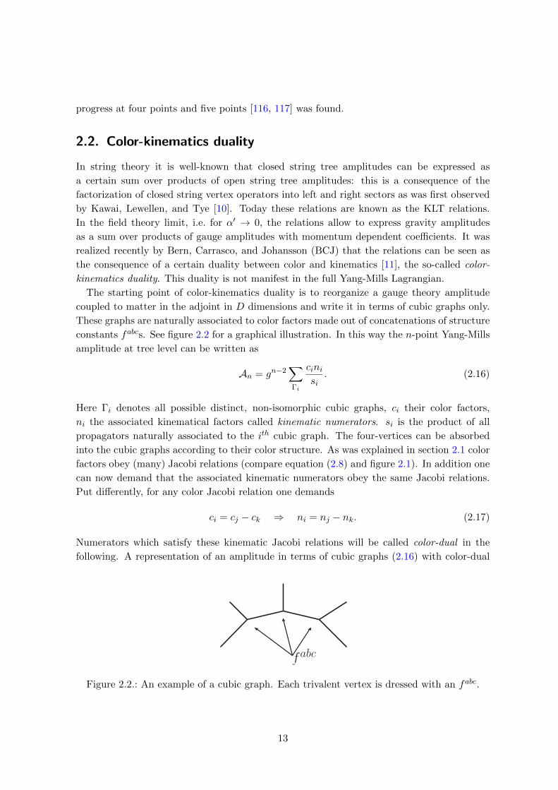
2.2. Color-kinematics duality
In string theory it is well-known that closed string tree amplitudes can be expressed as
a certain sum over products of open string tree amplitudes: this is a consequence of the
factorization of closed string vertex operators into left and right sectors as was first observed
by Kawai, Lewellen, and Tye [10]. Today these relations are known as the KLT relations.
In the field theory limit, i.e. for α′ → 0, the relations allow to express gravity amplitudes
as a sum over products of gauge amplitudes with momentum dependent coefficients. It was
realized recently by Bern, Carrasco, and Johansson (BCJ) that the relations can be seen as
the consequence of a certain duality between color and kinematics [11], the so-called color-
kinematics duality. This duality is not manifest in the full Yang-Mills Lagrangian.
The starting point of color-kinematics duality is to reorganize a gauge theory amplitude
coupled to matter in the adjoint in D dimensions and write it in terms of cubic graphs only.
These graphs are naturally associated to color factors made out of concatenations of structure
constants fabcs. See figure 2.2 for a graphical illustration. In this way the n-point Yang-Mills
amplitude at tree level can be written as
An = gn−2∑
Γi
cinisi
. (2.16)
Here Γi denotes all possible distinct, non-isomorphic cubic graphs, ci their color factors,
ni the associated kinematical factors called kinematic numerators. si is the product of all
propagators naturally associated to the ith cubic graph. The four-vertices can be absorbed
into the cubic graphs according to their color structure. As was explained in section 2.1 color
factors obey (many) Jacobi relations (compare equation (2.8) and figure 2.1). In addition one
can now demand that the associated kinematic numerators obey the same Jacobi relations.
Put differently, for any color Jacobi relation one demands
ci = cj − ck ⇒ ni = nj − nk. (2.17)
Numerators which satisfy these kinematic Jacobi relations will be called color-dual in the
following. A representation of an amplitude in terms of cubic graphs (2.16) with color-dual
fabc
Figure 2.2.: An example of a cubic graph. Each trivalent vertex is dressed with an fabc.
13

1 4
32
1
2 3
41 4
32
s−channel t−channel u−channel
Figure 2.3.: Cubic gluon graphs at four points. Note that these are not Feynman diagrams.
numerators will be called BCJ representation. As an explicit example for this consider a gluon
tree amplitude at four points. It consists of three cubic diagrams (see figure 2.3)
A4 =csnss
+ctntt
+cunuu
(2.18)
where s, t, and u are the usual four-point Mandelstam invariants. The color factors associated
to these graphs are
cs = fa1a2bfba3a4 ct = fa2a3bf
ba4a1 cu = fa1a3bfba4a2 . (2.19)
They obey the color Jacobi identity
cu = cs − ct. (2.20)
As was explained above, in order for the kinematic numerators to be color-dual, they have to
obey
nu = ns − nt. (2.21)
We will explicitly show how to obtain color-dual kinematic numerators based on a linear map
approach in chapter 4. Note that there is an analogous representation via cubic graphs for
color-ordered amplitudes. Here, one sums over all cubic diagrams that respect the ordering of
the external particles. For instance, the cubic representation for the four-point color-ordered
amplitude A(1234) will involve an s-channel and a t-channel cubic diagram. It is written in
this way as
A(1234) =nss
+ntt. (2.22)
In general, kinematic numerators are not unique. One can always shift the numerators by
some amount ∆i
ni → ni + ∆i. (2.23)
The scattering amplitude is invariant under these shifts if the gauge condition
∑
Γi
ci∆i
si= 0 (2.24)
holds. If the shifts also satisfy (2.17) the new numerators remain color-dual. This freedom
14

is generally referred to as generalized gauge freedom. The usual gauge transformations of
amplitudes are a subset of the generalized gauge transformations.
Additionally, kinematic numerators are antisymmetric when flipping the order at one of the
cubic vertices in the associated graph. This follows from the antisymmetry of the structure
constants under such a flip. This is nothing but a statement about Bose symmetry and in
this context it is usually referred to as vertex-flip antisymmetry
ci → −ci ⇔ ni → −ni (flipping the order at a cubic vertex). (2.25)
The main problem is finding color-dual numerators. Numerators for instance obtained
through standard Feynman rules will generically not satisfy Jacobi relations. However, for
theories in which color-dual numerators exist there will be a so-called generalized gauge
transformation that brings the numerators into a color-dual form (see also chapter 5 for a
take on numerators in terms of Feynman graphs). At tree level explicit all-multiplicity sets
of color-dual numerators have been found [126–128] proving that a color-dual representation
at tree level can always be found and color-kinematics holds. Moreover, as was recently
shown and will be explained below, one can in fact make color-kinematics duality manifest in
Yang-Mills at tree level in the self-dual and MHV sector [59].
The existence of color-dual numerators has powerful consequences. One is the existence of
additional relations: these are just the BCJ relations (2.15) introduced previously [11]. The
origin of these relations will be investigated in chapter 4 based on rephrasing color-kinematics
duality as a linear map. The second consequence is the double copy construction [11, 56]. This
construction makes it possible to obtain a gravity amplitude from a Yang-Mills amplitude in
BCJ representation (2.16) by simply replacing the color factors by another set of numerators
and the Yang-Mills coupling constant g by κ2 where κ is the gravitational coupling constant,
i.e.
An = gn−2∑
Γi
cinisi
⇒ Mn =(κ
2
)n−2∑
Γi
ninisi
. (2.26)
The field content of the resulting gravity theory is given by the outer product of the states
appearing in the Yang-Mills numerators. For instance, two sets of numerators from N = 4
super-Yang-Mills yield a gravity amplitude of N = 8 supergravity. However, numerators do
not have to be from the same gauge theory. One set of numerators could be from N = 0
Yang-Mills instead so that amplitudes in N = 4 supergravity will be obtained. Actually, only
one set of numerators has to be color-dual in the double copy construction [56]. A complete
classification of possible squarings in D = 4 can be found in [129]. Note that due to the gauge
condition (2.24) a generalized gauge transformation does not influence the outcome of the
double copy construction at tree level.
The double copy construction at tree level has been proven using recursive arguments under
the assumption that there are no non-trivial poles present in the numerators [56]. Moreover,
color-kinematics duality has been understood in terms of a hidden infinite dimensional kine-
matic Lie algebra [59, 130] in the self-dual and MHV sector at tree level. There has also
been recent progress for the systematic construction of numerators in [130–132] and on color-
kinematics duality in three dimensions [60, 133].
15

Conjecturally, there exists an extension of color-kinematics duality on the level of the loop
integrand [134] which is similar to tree level. One begins by rewriting the gauge theory
loop amplitude on the level of the integrand at the lth loop order as the sum over distinct
non-isomorphic cubic graphs
Al−loopn = gn−2+2l
∫ l∏
j=1
dDLj∑
Γi
1
Si
cinisi
. (2.27)
D denotes the space-time dimension and Si the symmetry factor of the ith cubic graph. The
term under the integral sign will in the following be called gauge theory integrand. Like at tree
level the color factors ci satisfy many Jacobi relations and one demands that the kinematic
numerators ni satisfy the same Jacobi relations. If this holds, i.e. the gauge theory integrand
can be expressed in a BCJ representation, then a corresponding gravity integrand can be
constructed by replacing the color factors by another set of numerators and the coupling
constants in the same way as at tree level, i.e.
Al−loopn = gn−2+2l
∫ l∏
j=1
dDLj∑
Γi
1
Si
cinisi
⇓M l−loopn =
(κ2
)n−2+2l∫ l∏
j=1
dDLj∑
Γi
1
Si
ninisi
.
(2.28)
Under the assumption that sets of color-dual numerators can always be found – which has
not been proven rigorously at loop level – the double copy construction follows from tree level
by unitarity [56].
Like at tree level the kinematic numerators are not unique at loop level neither. One can
shift the numerators according to ni → ni + ∆i and finds that the loop gauge amplitude
remains unchanged if the following condition holds
∫ l∏
j=1
dDLj∑
Γi
1
Si
ci∆i
si= 0. (2.29)
If desired the ∆i can be taken to be color-dual. This condition is not as strict as at tree level
since the integrand has only to satisfy integration to zero. In contrast to tree level this has
consequences for the double copy construction. It might be that the gauge condition does
not integrate to zero anymore after replacing color factors by another set of numerators since
the shifts are usually loop-momentum dependent. In other words it might occur that the
generalized gauge transformation enters the double copy. A very simplified version of such a
situation is ∫ ∞
−∞xdx = 0 whereas
∫ ∞
−∞x2dx 6= 0. (2.30)
Hence the question becomes: which terms vanish after integration? There are several cases
16
for which this can happen. The first case is that the integrand is merely a total derivative.
Consider for instance two terms that sum to zero after a shift of the integration variable for
one of them, i.e.
∫dDL
1
L2(L+ p1 + p2)2− 1
(L− p1)2(L+ p2)2= 0. (2.31)
The second possibility is that the integrand might have only vanishing D-dimensional uni-
tarity cuts then this integrand integrates to zero [135]. A nice example for this comes from
dimensional regularization for the integration of the constant 1 (or more generally speaking
for integrals with positive powers of loop momenta; see review [136] for more on this):
∫dDL 1 = 0. (2.32)
Vanishing of cuts is either purely algebraically or after a cut-condition-respecting shift in the
integration variable. The safe terms for the double copy construction are those that vanish
algebraically on cuts, i.e. whose loop momenta are fixed completely on the cuts: those do not
contribute after squaring.
There is yet another subtlety present for loop computations. In order to make color-
kinematics work it was found, e.g. in [51], one needs to include diagrams which integrate to
zero and which have a vanishing color factor. If these diagrams would have been neglected in
the double copy construction the resulting gravity amplitude would not have had the right
unitarity cuts. A more complete discussion of these subtleties would surely be interesting
as they are at the core of the double copy construction but this is beyond the scope of this
thesis. In the following it will always be assumed that color-dual numerators can be found
at any loop level and that one can safely disregard the subtlety involving generalized gauge
transformation.
There has been non-trivial evidence in support of color-kinematics duality and the double
copy at loop level in terms of explicit computations: four-point amplitudes up to four loops
in N = 8 supergravity [51, 137], five points up to two loops [138] have been computed using
the double copy construction. There have also been results in N = 4 supergravity up to three
loops [52, 53]. A color-dual form of the integrand of the 2-point form factor up to 4 loops,
3-point up to 2 loops in N = 4 super Yang-Mills has recently been derived in [55]. Moreover,
there was all-loop evidence from the IR-structure of gravity and Yang-Mills [139] and the
implications for color-kinematics duality and the double copy for deformations of Yang-Mills
theory by higher-dimension operators was discussed in [140].
Manifest color-kinematics in the self-dual sector
As was pointed out in [59] color-kinematics duality can be nicely made manifest at tree level
in the self-dual sector of Yang-Mills. This first step here is to realize that the self-dual sector
of Yang-Mills only has one three-vertex, i.e. amplitudes will be explicitly written in a cubic
representation. Moreover, any diagram in this sector immediately satisfies kinematic Jacobi
relations as will be explained below.
17

i+ j+
k−
=kηiηjη
〈η|ij|η〉faiajak
i− j−
k+
=kηiηjη
[η|ij|η]faiajak
i+ j+
k−l−
= iiηkη+jηlη(iη+lη)2
faial
bfbajak +
iηlη+jηkη(iη+kη)2
faiak
bfbajal
pi j = iδ
aiaj
p2e(+)i = [ηi]
〈ηi〉 e(−)i = 〈ηi〉
[ηi]
Figure 2.4.: Feynman rules of Yang-Mills in the light-cone gauge (given in terms of spinorhelicity. See [19] for a review.). e±i are the polarization vectors of the gluons. Forfuture convenience define X(i, j) = 〈η|ij|η〉, X(i, j) = [η|ij|η], and pη = 〈η|p|η].
The complete Yang-Mills Lagrangian in the light-cone gauge [141] is
L = tr(1
2A∂2A− ig
(∂w∂uA)
[A, ∂uA]− ig(∂w∂uA)
[A, ∂uA]− g2[A, ∂uA]1
∂2u
[A, ∂uA]). (2.33)
Here A is associated to the positive helicity gluon and A to the negative helicity gluon. The
light-cone gauge condition is Au = 0. The light-cone coordinates are defined by
u = t− z v = t+ z w = x+ iy w = x− iy (2.34)
and ∂2 = 2(∂u∂v − ∂w∂w). The Feynman rules in the light-cone gauge [59, 101] are depicted
in figure 2.4. The self-dual truncation of the full Lagrangian is simply
LSD = tr(1
2A∂2A− ig
(∂w∂uA)
[A, ∂uA]). (2.35)
Because this Lagrangian has only the trivalent (++−)–vertex there are only amplitudes with
helicity configuration (− + · · ·+) at tree level. In order to be color-dual, the numerators of
these amplitudes have to satisfy the same Jacobi relations as their corresponding color-factors
(2.8), i.e. for any triplet
f ijbfbkl = f jlbf
bik − f libf bkj (2.36)
the numerators coming from the (+ +−)–vertices have to obey
X(i, j)X(k, l) = X(j, l)X(i, k)−X(l, i)X(k, j) ∀{i, j, k, l} (2.37)
where we defined X(i, j) = 〈η|ij|η〉 and neglected prefactors as they are always the same.
18
After defining |x] = x|η〉 the above equation becomes
[ij][kl] = [j l][ik]− [li][kj] (2.38)
which is nothing but the Schouten identity (see (A.13)) for spinors and hence holds in gen-
eral for any {i, j, k, l} regardless of whether the spinors are on- or off-shell. Consequently,
amplitudes at tree level in the self-dual sector show explicitly the duality between color and
kinematics.
The analysis can be extended to the MHV level, i.e. for amplitudes with helicity configu-
ration (− − + · · ·+). The only way to construct these amplitudes is to consider in addition
to the (+ +−)–vertices either one (−−+)–vertex or one (−−++)–vertex. However, if one
imposes
|η〉 → |1〉 (2.39)
where particle 1 is taken to have negative helicity then this gauge choice forces particle 1 to
couple to a (−−+)–vertex. This can be easily understood since in this limit one has
e(−)1 → 0 1η = 〈1|1|η]→ 0 (2.40)
which can only be cancelled by a pole in 1 that is only present in the (−−+)–vertex. Hence
any MHV amplitude can be written in terms of (two types of) cubic vertices only: one
(−−+)–vertex and the rest (+ +−)–vertices. The analog of (2.37) becomes (again ignoring
common prefactors)
X(1, j)X(k, l) = X(j, l)X(1, k)− X(l, 1)X(k, j) (2.41)
with X(i, j) = [η|ij|η]. This can be written as (defining x|1〉 = |x])
[η1]([jη][kl]) = [η1]([kη][j l]− [ηl][kj]) (2.42)
which is again nothing but the Schouten identity, making color-kinematic duality manifest
also for tree-level MHV amplitudes.
2.3. BCFW shifts and on-shell recursion
On-shell recursion relations have been under heavy investigation in recent years. They have
first been derived for gauge theory tree amplitudes [34, 35] but were soon extended to gravity
tree amplitudes [142–144]. There has also been progress on finding on-shell recursion for
gauge theory integrands [38, 39, 145]. See [21] for a very nice review of the subject. For
simplicity only gluon amplitudes will be considered in this section unless otherwise stated.
The main idea behind on-shell recursion is to reconstruct a scattering amplitude from
the residues at its kinematic poles. To do so a complex parameter z is introduced into the
amplitude by shifting the momenta of any two external legs of the amplitude while keeping
19
momentum conservation intact:
pi = pi + zq pj = pj − zq. (2.43)
If the legs i and j are adjacent on a color trace of a color-ordered amplitude the shifts are
called adjacent shifts. If they are non-adjacent on a trace or if the shifted particles are on
different color traces, the shift will be called non-adjacent. The vector q is chosen such that
it keeps the masses of the external legs of the amplitudes invariant, i.e.
pi · q = pj · q = q · q = 0 (2.44)
giving two complex solutions for q. In this way the amplitude has been turned into a function
of a complex parameter z and the original – physical – amplitude A(z = 0) can be recovered
by Cauchy’s theorem, i.e. a contour integral around the origin
A(0) =1
2πi
∮
z=0
A(z)
zdz (2.45)
assuming that z = 0 is an isolated singularity. In this case the contour of integration can be
extended to infinity and the contour integral becomes (neglecting prefactors)
A(0) =
∮
z=0
A(z)
zdz = −
∑
residues
(finite z
)−∑
residue
(z =∞
). (2.46)
The residues at tree level for finite z are just products of lower point tree amplitudes summed
over all internal states. The residue at infinity lacks a similar physical interpretation but if
it can be shown to vanish (2.46) constitutes an on-shell recursion relation: the right hand
side only contains tree amplitudes with fewer legs. If a theory obeys recursion relations thus
depends on the behavior of the amplitude for z tending to infinity. If the fall-off of the
amplitude is fast enough, i.e. at least ∼ (z−1), the residue at infinity vanishes and a tree
level amplitude can be computed via recursion. There has been work on establishing on-shell
recursion in the presence of boundary terms [146] and only recently on-shell recursion for
Berends-Giele currents was introduced [147].
If the fall-off of the amplitude is better than ∼ (z−1) the recursion relation (2.46) can be
modified. For instance for a large-z behavior of ∼ (z−2) one can write
A(0) =
∮
z=0
(α− z)A(z)
αzdz = −
∑
residues
(finite z
)· f(pi), (2.47)
for some constant α. The residues on the right hand side are still the same products over lower
point tree amplitudes as before but now multiplied by an additional factor f(pi). The upshot
of this is two-fold: On the one hand, by an appropriate tuning of α, one can eliminate terms
in the recursion relation. This was for instance done in QED to obtain a compact recursion
formula [148]. On the other hand the improved behavior under BCFW shifts implies the
existence of bonus relations among the amplitudes. For a gravity example consider [149].
20
Improved large-z behavior was also key in [121] to prove the tree-level BCJ relations in field
theory.
There are several ways to analyze the large-z behavior of an amplitude. All of them
are based on powercounting, i.e. tracing explicit powers of z in Feynman diagrams. In the
following the shortest (simply connected) path between the two shifted legs along which the z-
dependence flows will be called hard line. The large-z behavior of a Yang-Mills tree amplitude
for the shift of two color-adjacent particles labelled i and i+ 1 is of the form [145, 150]
limz→∞
A(z) ∼ εµi (z)ενi+1(z)(zηµνf(1/z) + z0Bµν(1/z) +O(1/z)
)(2.48)
with f and Bµν polynomial functions in z−1. Moreover, Bµν is antisymmetric in its indices
and εi are the z-dependent polarization vectors of the shifted legs. This result holds for all
Yang-Mills theories minimally coupled to fermionic and scalar matter with possible scalar
potential or Yukawa terms in D ≥ 4 [151]. Taking into account the explicit z scaling of
the polarization vectors (which can be constructed using a basis of the vectors pi, pi+1, q, q∗
[150]) one finds that the amplitude shows ‘good’ behavior, i.e. 1/z-scaling, under (−,±)-gluon
and (+,+)-gluon shifts with (·, ·) denoting the helicities of the shifted adjacent gluons. For
a (+,−)-shift the amplitude will scale like ∼ (z3). Thus the former three cases allow for
on-shell recursion, the latter not.
A very lucid way to obtain (2.48) for tree level amplitudes is to split the Yang-Mills fields
into z-dependent “hard” fields aµ and z-independent soft fields Aµ. In this way one treats the
BCFW shifted particles as particles with very large momenta flying through a background
given by the unshifted particles having small momentum. This can be nicely formulated in
terms of the background field method [152]. The quadratic part of the Lagrangian of the hard
fields a reads
L = −1
4TrDνaµD
νaµ +i
2Tr[aµ, aν ]Fµν [A] (2.49)
where the equations of motions of the soft fields have been used in the derivation to eliminate
the terms linear in a. In other words this derivation is only valid at tree level. The hard fields
have been put into the background field version of the Feynman-’t Hooft gauge. As only the
hard fields carry z-dependent momentum the complete z-dependence is now exclusively in
the first term of the Lagrangian. As can be seen from the Lagrangian it is proportional to z
and contains a metric contraction between the hard fields. The hard propagator is given by
: aµaν := −iηµνp2
(2.50)
and consequently scales as ∼ (z−1). Hence any Feynman graph with an insertion from the
second term of the above Lagrangian will be suppressed by one power in z and moreover be
antisymmetric in the hard fields: these observations combined yield (2.48). The powercount-
ing can be simplified further using the gauge freedom of the background fields to impose the
‘spacecone’ gauge which we call Arkani-Hamed-Kaplan (AHK) gauge [141, 150]
q ·A = 0 (2.51)
21
with q being the BCFW shift vector introduced in (2.43). This gauge choice is very handy and
quite natural as the propagator of the soft fields is now orthogonal to q and thus eliminates
most of the z-dependence from the three-vertices.
Another way to do the powercounting is to implement AHK directly for all particles, thereby
not distinguishing between hard and soft particles. The advantage of this approach is that no
on-shell conditions are necessary and as a consequence the validity of (2.48) can be extended
also to the level of the integrand to any loop order [145] as will be seen below. The rederivation
of (2.48) from [145] will be repeated here as a warm-up as it is the basis to obtain the behavior
of the amplitude/integrand for color non-adjacent large-z shifts in chapter 5.
The AHK gauge (2.51) will be chosen for all external particles except for the two shifted
ones. This would not be a valid gauge choice because q is orthogonal to the external momenta
of the shifted legs. For the shifted legs one has
p · ε(p) = (p± zq) · ε(p) = 0 ⇒ q · ε(p) = ∓p · ε(p)z
. (2.52)
The AHK propagator is a spacecone propagator given by
Gµν(p) =−ip2
(ηµν −
qµpν + qνpµq · p
). (2.53)
It is orthogonal to q and collapses when contracted into its momentum, i.e.
qµGµν(p) = 0
pµGµν(p) =iqνq · p.
(2.54)
To do the powercounting, consider the hard line part of a Feynman graph. The unshifted legs
will be left arbitrary; thus the result will hold on the level of the integrand of Yang-Mills to
any loop order. Along the hard line the AHK propagator scales as ∼ (z0)
Ghardµν (p) ∼ 2z
p2 ± 2zq · p(qµqνq · p
)+O(1/z). (2.55)
Due to its dependence on two qs it will hardly ever contribute since q contracted into any
unshifted leg vanishes. Moreover, the three-vertices are in fact independent of z (with one
exception mentioned below) because of the AHK gauge.
The leading diagram for an adjacent shift is the three-vertex to which the two shifted legs
attach directly. The diagram will scale like a metric times z as can be easily shown using the
Feynman rules in appendix B. Note that there is a subtlety involved here: the momentum of
the off-shell leg is p1 + p2 and hence an AHK propagator attaching to this leg diverges since
these two momenta are orthogonal to q. In other words the AHK gauge choice is singular
for this class of graphs. Fortunately, the gauge singularity can be avoided by imposing an
auxiliary gauge [145] and one finds the leading term in (2.48).
The subleading behavior, i.e. the ∼ (z0) term of (2.48), arises from the graphs depicted in
figure 2.5. Using the Feynman rules of the appendix the two diagrams can be viewed as an
22

Figure 2.5.: The Feynman diagrams contributing at O(z0) for adjacent shifts. Hats denotethe shifted legs.
effective four-vertex that is antisymmetric in the adjacently shifted legs for large z
4V effectiveµνρσ = iz0
(ηµρηνσ − ηµσηνρ −
1
2ηµνηρσ
)+O(1/z). (2.56)
Note that actually the last term is only given for completeness. It is a metric contraction
between the shifted legs and can be seen as a subleading contribution of f in (2.48). Unless
otherwise stated such terms will be neglected in the following. All other hard line graphs with
more hard propagators will be z-suppressed and do not contribute at this order. Combining
the above results then yields (2.48).
For gravity theories similar recursion relations can be derived at tree level. This is somewhat
startling as by inspecting for instance Feynman rules from Einstein gravity [153] one would
think that a n-point gravity tree amplitude scales like ∼ (zn−2) in the large-z limit. However,
explicit examples show the opposite and explicit recursion has been constructed for Einstein
gravity and its supersymmetric extensions [142–144]. An explicit analysis employing the
background field method mentioned above could show that the gravity scaling is actually just
a double copy of the Yang-Mills tree amplitude scaling [150], i.e.
limz→∞
Mn(z) ∼[εµi (z)εµi (z)
][ενi+1(z)ενi+1(z)
](zηµνf(1/z) + z0Bµν(1/z) +O(1/z)
)
(zηµνf(1/z) + z0Bµν(1/z) +O(1/z)
) (2.57)
where B is as before an antisymmetric tensor. The product of polarization tensors in brackets
belongs to the graviton, dilaton, and two-form. In other words the gravity amplitude exhibits
drastic cancellations with respect to the expectation from Feynman diagrams. What is the
mechanism behind these cancellations in the sum over Feynman diagrams? Does the result
extend to the level of the integrand as is known for gauge theory amplitudes? These questions
will be answered in chapter 4.
2.4. Generalized inverses
Generalized inverses will be a central theme in chapter 4 in the study of kinematic numerators.
Originally, due to Moore and later independently Penrose [154, 155], generalized inverses were
introduced to extend the notion of invertibility to rectangular matrices and singular matrices
23
and in addition to more general linear maps. In the following a lightning review of the
elements necessary for this thesis will be given. A broader introduction can be found in [156].
Matrices are a nice tool to treat systems of linear equations efficiently. These are usually
denoted as
Ax = b (2.58)
for some matrix A and x, b appropriate vectors. A linear system is uniquely solvable if A is
an n× n matrix with full rank. The inverse is given by A−1 so that
A−1A = 1n×n = AA−1 (2.59)
holds and the solution to the linear system can be obtained by
x = A−1b. (2.60)
If A were singular or rectangular an inverse in the above sense does not exist. This corresponds
to situations where the system is either under- or overdetermined. Nonetheless, it can still
have solutions which can be obtained using generalized inverses. Formally, the generalized
inverse of an n ×m matrix A is a m × n matrix denoted by A+ which obeys the following
defining property
AA+A = A. (2.61)
This condition reduces to A+ = A−1 for full rank matrices. For A being rectangular or singular
the linear system Ax = b can only have solutions if the following consistency condition holds
AA+b = b. (2.62)
If this is fulfilled the general solution to (2.58) is given by
x = A+b+ (1−A+A)v (2.63)
with v some n-dimensional vector. The second term in the equation spans the kernel of A,
i.e.
ker A = {(1−A+A)v|v ∈ Cn} (2.64)
and it can be checked easily that (2.63) indeed solves (2.58).
Note that the generalized inverse is not quite unique as one can always add terms from the
kernel of A without violating (2.61). In other words if A+ is a generalized inverse so is
A+′ = A+ + (1−A+A)V +W (1−AA+) (2.65)
for appropriate m × m and n × n matrices V , W . A worked out example involving the
generalized inverse will be given in chapter 4 in terms of scattering amplitudes.
The generalized inverse above can also be extended to include more general linear maps;
these maps do not necessarily have to be between vector spaces over fields. Denote such a
24
map now by C. As a simple example consider the case of a linear map given by
C : V →W with V = Z W = Z mod 2 (2.66)
where Z denotes the ring of integers. A linear map from V to W is then given by
Cx ∼ b, x ∈ Z, b ∈ Z mod 2 (2.67)
with ∼ denoting equality on W . The generalized inverse C+ is now a map from W to V
satisfying
CC+Cx ∼ Cx ∀x ∈ Z (2.68)
As a concrete example for C take multiplication by 2, i.e.
C(x) = 2x. (2.69)
Obviously, for Cx = 2x ∼ b to have a solution, b can only take the value 0. In this case
any one-to-one map C+ : W → V will satisfy (2.68). Expressing this more formally, the
consistency condition for this system to be invertible in the generalized sense is given by
CC+b ∼ b (2.70)
which is indeed satisfied for b ∼ 0 only. In this case this condition is necessary and sufficient.
Hence, the most general solution to this system is then given by
x = C+b+ ker C (2.71)
with the kernel arising due to the different dimensionalities of V and W . In other words: the
maps are many-to-one.
Note that it is quite special that the consistency condition (2.70) is necessary and sufficient.
It might very well be that more conditions are needed as the maps involved are many-to-one
as explained above. The more general consistency condition is that for every linear map
D : W →W with
D(Cx) ∼ 0 (2.72)
it follows
D(b) ∼ 0. (2.73)
The general solution is then again given in terms of (2.71). As before C+ is not unique. One
can add terms from the kernel, i.e. if C+ satisfies (2.68), so does
C+ → C+ +D1 +D2 (2.74)
for D1, D2 satisfying
CD1x ∼ 0 and D2Cx ∼ 0. (2.75)
This is nothing but the generalization of (2.65).
25

26
3. Color-kinematics duality for one-loop
rational amplitudes
In this chapter it will be shown that color-kinematics duality is manifest at the one-loop
level in Yang-Mills theory for amplitudes with all particles of either the same helicity or
with one opposite to the other. These one-loop amplitudes are special in that they have no
four-dimensional unitarity cuts, i.e. they do not contain logarithms in four dimensions after
integration. They are rational functions of external momenta and polarizations only and
hence called rational amplitudes.
First, we will consider rational all-plus amplitudes. These are computed in the self-dual
sector of Yang-Mills. As was already seen in the previous chapter, this sector is particularly
nice because it only has one cubic vertex making color-kinematics duality manifest. Going be-
yond the self-dual sector, it will be explained that also one-minus amplitudes can be brought
into a color-kinematics duality manifest form by a specific choice of gauge. As a concrete ap-
plication of the duality the corresponding one-loop gravity amplitudes in N = 0 supergravity
will be calculated at four points using the double copy construction. In this way, this chapter
extends the tree-level results of [59] outlined in section 2.2 to one loop.
3.1. Manifestly color-dual integrands at one loop
As in the tree level case it will be useful to investigate self-dual Yang-Mills by going to light-
cone coordinates. The corresponding formalism and the Lagrangian were already presented
in chapter 2. The complete Lagrangian is reproduced here for convenience
L = tr(1
2A∂2A− ig
(∂w∂uA)
[A, ∂uA]− ig(∂w∂uA)
[A, ∂uA]− g2[A, ∂uA]1
∂2u
[A, ∂uA]).
Recall that A and A denote positive, negative gluons respectively. The self-dual part of
this Lagrangian is given by the first two terms and it gives rise to only the (+ + −)–vertex.
Consequently, the only amplitudes one can compute in the self-dual sector at the one-loop level
are all-plus amplitudes. It was already shown in section 2.2 that numerators constructed out
of the (++−)–vertex satisfy the same Jacobi relations as their corresponding color structures
at tree level and that this was nothing but a consequence of the Schouten identities; there is
no reference to on- or off-shellness of the spinors involved and hence this result immediately
extends also to one-loop; in other words the self-dual sector of Yang-Mills at one-loop exhibits
manifestly color-kinematics duality.
Next, consider one-loop amplitudes with one external negative helicity gluon. The following
observations are very closely related to those about the connection of the self-dual sector and
27
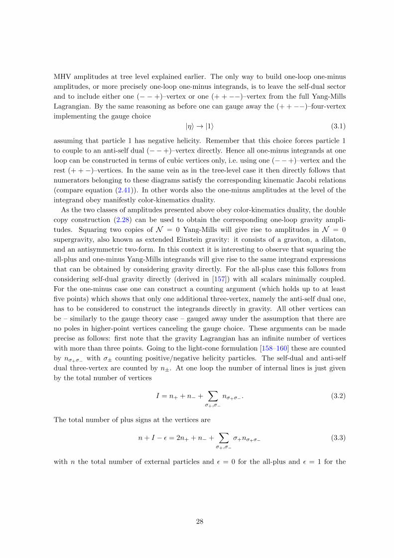
MHV amplitudes at tree level explained earlier. The only way to build one-loop one-minus
amplitudes, or more precisely one-loop one-minus integrands, is to leave the self-dual sector
and to include either one (− − +)–vertex or one (+ + −−)–vertex from the full Yang-Mills
Lagrangian. By the same reasoning as before one can gauge away the (+ +−−)–four-vertex
implementing the gauge choice
|η〉 → |1〉 (3.1)
assuming that particle 1 has negative helicity. Remember that this choice forces particle 1
to couple to an anti-self dual (−−+)–vertex directly. Hence all one-minus integrands at one
loop can be constructed in terms of cubic vertices only, i.e. using one (−−+)–vertex and the
rest (+ +−)–vertices. In the same vein as in the tree-level case it then directly follows that
numerators belonging to these diagrams satisfy the corresponding kinematic Jacobi relations
(compare equation (2.41)). In other words also the one-minus amplitudes at the level of the
integrand obey manifestly color-kinematics duality.
As the two classes of amplitudes presented above obey color-kinematics duality, the double
copy construction (2.28) can be used to obtain the corresponding one-loop gravity ampli-
tudes. Squaring two copies of N = 0 Yang-Mills will give rise to amplitudes in N = 0
supergravity, also known as extended Einstein gravity: it consists of a graviton, a dilaton,
and an antisymmetric two-form. In this context it is interesting to observe that squaring the
all-plus and one-minus Yang-Mills integrands will give rise to the same integrand expressions
that can be obtained by considering gravity directly. For the all-plus case this follows from
considering self-dual gravity directly (derived in [157]) with all scalars minimally coupled.
For the one-minus case one can construct a counting argument (which holds up to at least
five points) which shows that only one additional three-vertex, namely the anti-self dual one,
has to be considered to construct the integrands directly in gravity. All other vertices can
be – similarly to the gauge theory case – gauged away under the assumption that there are
no poles in higher-point vertices canceling the gauge choice. These arguments can be made
precise as follows: first note that the gravity Lagrangian has an infinite number of vertices
with more than three points. Going to the light-cone formulation [158–160] these are counted
by nσ+σ− with σ± counting positive/negative helicity particles. The self-dual and anti-self
dual three-vertex are counted by n±. At one loop the number of internal lines is just given
by the total number of vertices
I = n+ + n− +∑
σ+,σ−
nσ+σ− . (3.2)
The total number of plus signs at the vertices are
n+ I − ε = 2n+ + n− +∑
σ+,σ−
σ+nσ+σ− (3.3)
with n the total number of external particles and ε = 0 for the all-plus and ε = 1 for the
28
one-minus case. The total number of minus signs at the vertices is given by
ε+ I = n+ + 2n− +∑
σ+,σ−
σ−nσ+σ− . (3.4)
Subtracting the first from the third equation leads to
ε = n− +∑
σ+,σ−
(σ− − 1)nσ+σ− . (3.5)
Consider now the all-plus case, i.e. ε = 0. The only way the above equation (3.5) holds is if the
two terms vanish independently, i.e. if neither the anti-self dual nor any of the higher-point
vertices are present. Thus the all-plus gravity integrand is only built from self-dual vertices
only as already indicated by the double copy construction. For the one-minus case, i.e. ε = 1
one needs to consider either one (−−+)–vertex (n− = 1) or a higher point vertex with two
negative helicity particles (nσ+2 = 1). However, as was explained above for Yang-Mills we
can restrict ourselves to the (− − +)–vertex by choosing |η〉 → |1〉 where again is assumed
that 1 carries negative helicity. This choice will eliminate all higher-point vertices nσ+2 under
the assumption that they do not have any poles in 〈η1〉 which has been proven up to five
points [160]. These two observations give in fact a Lagrangian based proof of the double copy
conjecture in the helicity-equal sector and in the one-helicity unequal sector up to at least
five points at one loop though it seems likely that the latter holds beyond five points.
The differences between self-dual gravity and self-dual N = 0 supergravity are very small;
in fact for rational amplitudes the difference only lies in the available states running in the
loop. For self-dual N = 0 there are two more states available so that the amplitudes differ by
a factor of 2. This is a consequence of supersymmetric Ward identities which allow to replace
gravitons (and other massless particles) running in the loop by massless scalars [161–163].
The rational gravity amplitudes are thus given by
M (1−loop),any statesn (1±, 2+, ..., n+) = NsM
(1−loop),scalarsn (1±, 2+, ..., n+) (3.6)
with Ns the number of states running in the loop (bosonic minus fermionic). For pure gravity
Ns = 2 (two graviton states) and for N = 0 it follows Ns = 4 (two graviton states, a dilaton,
an antisymmetric two-form).
3.2. Examples
To illustrate the general arguments presented above, we will now explicitly show some ex-
amples. In particular, rational four-point one-loop gravity amplitudes will be computed to
illustrate the double copy procedure. For the light-cone Feynman rules used in the following,
see figure 2.4.
Higher-point amplitudes obtained in the same way will obviously satisfy kinematic consis-
tency conditions, i.e. as they are rational they will not have any four-dimensional cuts and
applying (a number of) collinear limits they will reduce to the four-point result.
29
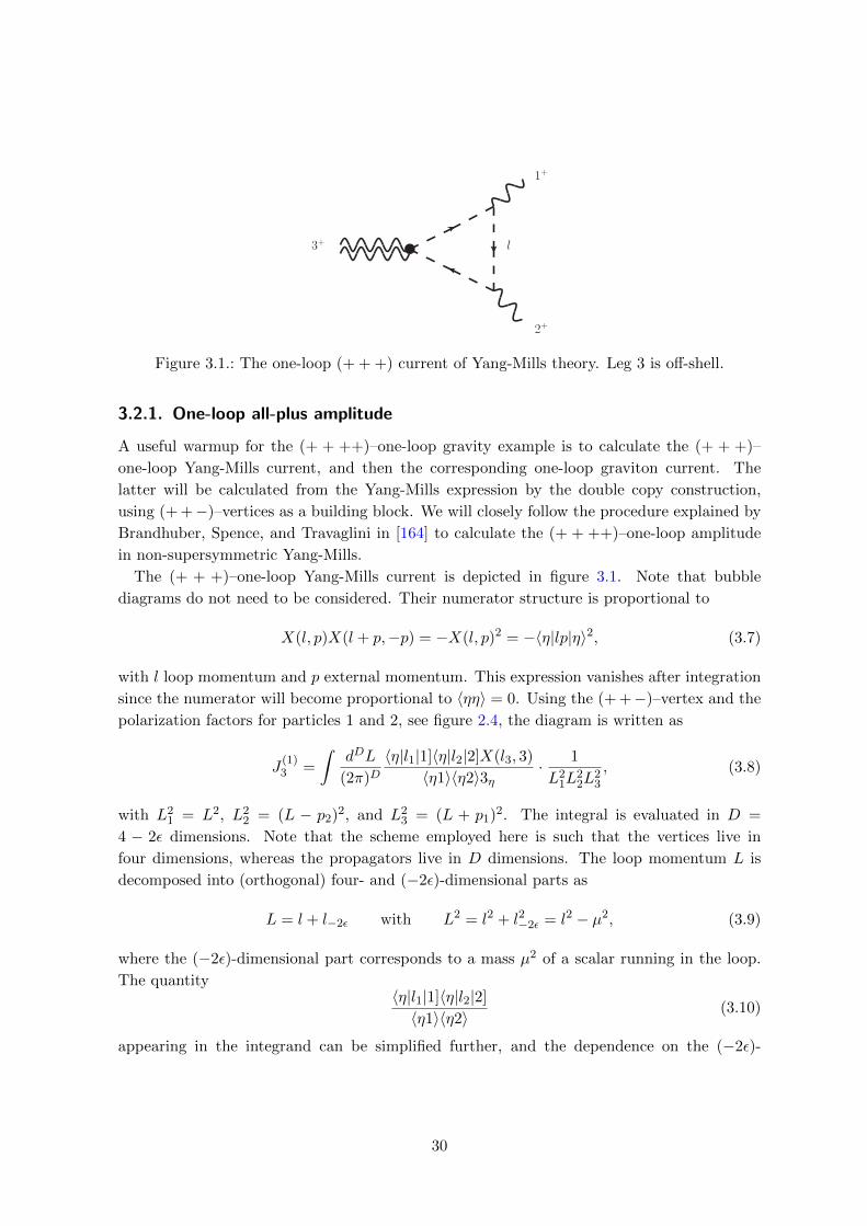
3+
1+
2+
l
Figure 3.1.: The one-loop (+ + +) current of Yang-Mills theory. Leg 3 is off-shell.
3.2.1. One-loop all-plus amplitude
A useful warmup for the (+ + ++)–one-loop gravity example is to calculate the (+ + +)–
one-loop Yang-Mills current, and then the corresponding one-loop graviton current. The
latter will be calculated from the Yang-Mills expression by the double copy construction,
using (+ +−)–vertices as a building block. We will closely follow the procedure explained by
Brandhuber, Spence, and Travaglini in [164] to calculate the (+ + ++)–one-loop amplitude
in non-supersymmetric Yang-Mills.
The (+ + +)–one-loop Yang-Mills current is depicted in figure 3.1. Note that bubble
diagrams do not need to be considered. Their numerator structure is proportional to
X(l, p)X(l + p,−p) = −X(l, p)2 = −〈η|lp|η〉2, (3.7)
with l loop momentum and p external momentum. This expression vanishes after integration
since the numerator will become proportional to 〈ηη〉 = 0. Using the (+ +−)–vertex and the
polarization factors for particles 1 and 2, see figure 2.4, the diagram is written as
J(1)3 =
∫dDL
(2π)D〈η|l1|1]〈η|l2|2]X(l3, 3)
〈η1〉〈η2〉3η· 1
L21L
22L
23
, (3.8)
with L21 = L2, L2
2 = (L − p2)2, and L23 = (L + p1)2. The integral is evaluated in D =
4 − 2ε dimensions. Note that the scheme employed here is such that the vertices live in
four dimensions, whereas the propagators live in D dimensions. The loop momentum L is
decomposed into (orthogonal) four- and (−2ε)-dimensional parts as
L = l + l−2ε with L2 = l2 + l2−2ε = l2 − µ2, (3.9)
where the (−2ε)-dimensional part corresponds to a mass µ2 of a scalar running in the loop.
The quantity〈η|l1|1]〈η|l2|2]
〈η1〉〈η2〉 (3.10)
appearing in the integrand can be simplified further, and the dependence on the (−2ε)-
30

dimensional subspace can be extracted. To do so, write it as
〈η|l112l1|η〉〈η1〉〈η2〉〈12〉 = −l21
[12]
〈12〉 −2(l1 · p1)〈η|1 l1|η〉〈η1〉〈η2〉〈12〉 − 2(l1 · p2)〈η|l1 2|η〉
〈η1〉〈η2〉〈12〉 , (3.11)
where the definition of the Clifford algebra has been used on /l1 /1 and /2 /l1 on the left hand
side. The scalar products can be expressed as the difference of propagators
2(l1 · p1) = l23 − l21 = L23 − L2
1 and 2(l1 · p2) = L21 − L2
2, (3.12)
and l21 = L21 + µ2 by (3.9). Finally, one obtains
〈η|l1|1]〈η|l2|2]
〈η1〉〈η2〉 = −µ2 [12]
〈12〉 +Q
〈12〉 ; Q = L21
〈η|l3(1 + 2)|η〉〈η1〉〈η2〉 +L2
2
〈η|l1|1]
〈η2〉 +L23
〈η|l1|2]
〈η1〉 . (3.13)
The one-loop current becomes
J(1)3 (+ + +) =
∫dDL
(2π)D
(− µ2 [12]
〈12〉 +Q
〈12〉)X(l3, 3)
3η· 1
L21L
22L
23
. (3.14)
Upon standard one-loop integration of this expression, one finds that only the part propor-
tional to µ2 survives. The µ2 dependence can be related to an integral in D + 2 dimensions
via the identity [165]
∫dDL
(2π)D(µ2)rf(l, µ2) = −ε(1− ε)...(r − 1− ε)(4π)r
∫dD+2rL
(2π)D+2rf(l, µ2) (3.15)
where again l and µ2 denote the four- and (−2ε)-dimensional components of L. Eventually,
the result is
J(1)3 (+ + +) =
i
(4π)2−ε ·Γ(1 + ε)Γ(1− ε)2
Γ(4− 2ε)(−p23)ε· [12]2
〈12〉 ·〈η1〉〈η2〉
3η. (3.16)
Next consider gravity. It was shown before that the color-kinematics duality is manifest in
self-dual gauge theory, so one can just apply the double copy by squaring the numerator (that
is, the integrand excluding the propagators) in equation (3.8). Again, one does not need to
consider bubble topologies, which vanish upon integration. The three-graviton all-plus one-
loop current is given by
J (1)3 (+ + +) =
∫dDL
(2π)D
(〈η|l1|1]〈η|l2|2]X(l3, 3)
〈η1〉〈η2〉3η
)2· 1
L21L
22L
23
, (3.17)
which will become, using (3.13),
J (1)3 (+ + +) =
∫dDL
(2π)D
(− µ2 [12]
〈12〉 +Q
〈12〉)2X(l3, 3)2
32η
· 1
L21L
22L
23
. (3.18)
Expanding out the integrand gives terms proportional to µ4, µ2, and µ0. It can be shown
31
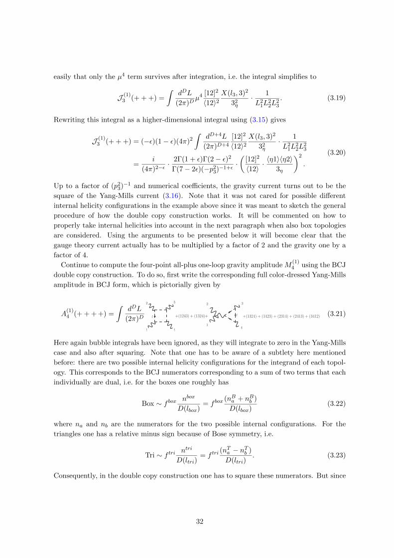
easily that only the µ4 term survives after integration, i.e. the integral simplifies to
J (1)3 (+ + +) =
∫dDL
(2π)Dµ4 [12]2
〈12〉2X(l3, 3)2
32η
· 1
L21L
22L
23
. (3.19)
Rewriting this integral as a higher-dimensional integral using (3.15) gives
J (1)3 (+ + +) = (−ε)(1− ε)(4π)2
∫dD+4L
(2π)D+4
[12]2
〈12〉2X(l3, 3)2
32η
· 1
L21L
22L
23
=i
(4π)2−ε ·2Γ(1 + ε)Γ(2− ε)2
Γ(7− 2ε)(−p23)−1+ε
·(
[12]2
〈12〉 ·〈η1〉〈η2〉
3η
)2
.
(3.20)
Up to a factor of (p23)−1 and numerical coefficients, the gravity current turns out to be the
square of the Yang-Mills current (3.16). Note that it was not cared for possible different
internal helicity configurations in the example above since it was meant to sketch the general
procedure of how the double copy construction works. It will be commented on how to
properly take internal helicities into account in the next paragraph when also box topologies
are considered. Using the arguments to be presented below it will become clear that the
gauge theory current actually has to be multiplied by a factor of 2 and the gravity one by a
factor of 4.
Continue to compute the four-point all-plus one-loop gravity amplitude M(1)4 using the BCJ
double copy construction. To do so, first write the corresponding full color-dressed Yang-Mills
amplitude in BCJ form, which is pictorially given by
A(1)4 (+ + + +) =
∫dDL
(2π)D
1
2 3
4
l +(1243) + (1324)+ +(1324) + (1423) + (2314) + (2413) + (3412)l
1
2 3
4
(3.21)
Here again bubble integrals have been ignored, as they will integrate to zero in the Yang-Mills
case and also after squaring. Note that one has to be aware of a subtlety here mentioned
before: there are two possible internal helicity configurations for the integrand of each topol-
ogy. This corresponds to the BCJ numerators corresponding to a sum of two terms that each
individually are dual, i.e. for the boxes one roughly has
Box ∼ f box nbox
D(lbox)= f box
(nBa + nBb )
D(lbox)(3.22)
where na and nb are the numerators for the two possible internal configurations. For the
triangles one has a relative minus sign because of Bose symmetry, i.e.
Tri ∼ f tri ntri
D(ltri)= f tri
(nTa − nTb )
D(ltri). (3.23)
Consequently, in the double copy construction one has to square these numerators. But since
32
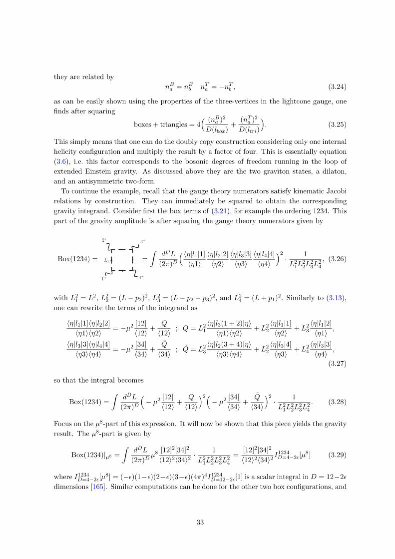
they are related by
nBa = nBb nTa = −nTb , (3.24)
as can be easily shown using the properties of the three-vertices in the lightcone gauge, one
finds after squaring
boxes + triangles = 4( (nBa )2
D(lbox)+
(nTa )2
D(ltri)
). (3.25)
This simply means that one can do the doubly copy construction considering only one internal
helicity configuration and multiply the result by a factor of four. This is essentially equation
(3.6), i.e. this factor corresponds to the bosonic degrees of freedom running in the loop of
extended Einstein gravity. As discussed above they are the two graviton states, a dilaton,
and an antisymmetric two-form.
To continue the example, recall that the gauge theory numerators satisfy kinematic Jacobi
relations by construction. They can immediately be squared to obtain the corresponding
gravity integrand. Consider first the box terms of (3.21), for example the ordering 1234. This
part of the gravity amplitude is after squaring the gauge theory numerators given by
Box(1234) = L1
2+ 3+
4+1+
=
∫dDL
(2π)D
(〈η|l1|1]
〈η1〉〈η|l2|2]
〈η2〉〈η|l3|3]
〈η3〉〈η|l4|4]
〈η4〉)2· 1
L21L
22L
23L
24
, (3.26)
with L21 = L2, L2
2 = (L− p2)2, L23 = (L− p2 − p3)2, and L2
4 = (L+ p1)2. Similarly to (3.13),
one can rewrite the terms of the integrand as
〈η|l1|1]〈η|l2|2]
〈η1〉〈η2〉 = −µ2 [12]
〈12〉 +Q
〈12〉 ; Q = L21
〈η|l3(1 + 2)|η〉〈η1〉〈η2〉 + L2
2
〈η|l1|1]
〈η2〉 + L23
〈η|l1|2]
〈η1〉 ,
〈η|l3|3]〈η|l4|4]
〈η3〉〈η4〉 = −µ2 [34]
〈34〉 +Q
〈34〉 ; Q = L23
〈η|l2(3 + 4)|η〉〈η3〉〈η4〉 + L2
2
〈η|l3|4]
〈η3〉 + L24
〈η|l3|3]
〈η4〉 ,
(3.27)
so that the integral becomes
Box(1234) =
∫dDL
(2π)D
(− µ2 [12]
〈12〉 +Q
〈12〉)2(− µ2 [34]
〈34〉 +Q
〈34〉)2· 1
L21L
22L
23L
24
. (3.28)
Focus on the µ8-part of this expression. It will now be shown that this piece yields the gravity
result. The µ8-part is given by
Box(1234)|µ8 =
∫dDL
(2π)Dµ8 [12]2[34]2
〈12〉2〈34〉2 ·1
L21L
22L
23L
24
=[12]2[34]2
〈12〉2〈34〉2 I1234D=4−2ε[µ
8] (3.29)
where I1234D=4−2ε[µ
8] = (−ε)(1−ε)(2−ε)(3−ε)(4π)4I1234D=12−2ε[1] is a scalar integral in D = 12−2ε
dimensions [165]. Similar computations can be done for the other two box configurations, and
33

one finds
Box|µ8 =[12]2[34]2
〈12〉2〈34〉2(I1234D=4−2ε[µ
8] + I1243D=4−2ε[µ
8] + I1324D=4−2ε[µ
8]), (3.30)
which is the one-loop four-point all-plus gravity amplitude as computed by Bern et al [162] up
to a factor of four. However, the factor of four follows from the discussion at the beginning of
this section (3.25) so that the µ8 piece does actually give the correct all-plus gravity amplitude
for N = 0 supergravity.
In order to check that this computation gives the correct result, it must be verified that
the µ6, µ4, µ2, and µ0 terms of the box integral (3.28) and the triangle integrals cancel in the
sum, i.e
Box|µ6 + Box|µ4 + Box|µ2 + Box|µ0 + Triangles?= 0 (3.31)
The box terms can be extracted from (3.28). The triangle diagram contributions are obtained
by putting together a (+ +−)–tree-level gravity current, i.e. the square of a one-leg off-shell
(++−)–vertex from figure 2.4, and the one-loop all-plus current (3.20). After a bit of algebra,
one finds
Tri(1234) =
3+
L1
1+
2+
4+
=i
(4π)2−ε2Γ(1 + ε)Γ(2− ε)2
Γ(7− 2ε)(−s12)ε〈η|34|η〉4
〈12〉2〈34〉2∏4i=1〈ηi〉2
. (3.32)
The other triangle configurations are obtained by permutation of the external legs. Finally,
after evaluating all these integrals, we checked numerically (up to and including O(ε2) in
dimensional regularization) that the terms in (3.31) indeed add up to zero.
In summary, we have calculated the one-loop (+ + ++) N = 0 supergravity amplitude
M(1)4 using the BCJ double copy construction, and reproduced the well-known expression
M(1)4 (+ + + +) = 4 Box|µ8 = 4
[12]2[34]2
〈12〉2〈34〉2(I1234D=4−2ε[µ
8] + I1243D=4−2ε[µ
8] + I1324D=4−2ε[µ
8]).
(3.33)
3.2.2. One-loop one-minus amplitude
As another interesting example of numerators satisfying the color-kinematics duality, the one-
minus one-loop gravity three-current and four-point amplitude will be calculated. To do so,
one can reuse most parts of the machinery from the previous computation. To make the
color-kinematics duality manifest, the gauge choice introduced earlier will be implemented
|η〉 = |1〉, (3.34)
where particle 1 has negative helicity particle. This choice eliminates four-point vertices and
forces particle 1 to couple to a (−−+)–vertex.
We begin with the (− + +)–one-loop current as it is a building block for the one-minus
four-point amplitude (see figure 3.2). Using the rules of figure 2.4, including the polarization
34
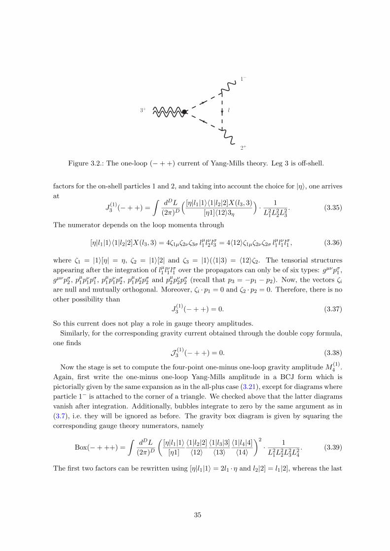
3+
1−
2+
l
Figure 3.2.: The one-loop (−+ +) current of Yang-Mills theory. Leg 3 is off-shell.
factors for the on-shell particles 1 and 2, and taking into account the choice for |η〉, one arrives
at
J(1)3 (−+ +) =
∫dDL
(2π)D
( [η|l1|1〉〈1|l2|2]X(l3, 3)
[η1]〈12〉3η
)· 1
L21L
22L
23
. (3.35)
The numerator depends on the loop momenta through
[η|l1|1〉〈1|l2|2]X(l3, 3) = 4ζ1µζ2νζ3σ lµ1 lν2 lσ3 = 4〈12〉ζ1µζ2νζ2σ l
µ1 lν1 lσ1 , (3.36)
where ζ1 = |1〉[η| = η, ζ2 = |1〉[2| and ζ3 = |1〉(〈1|3) = 〈12〉ζ2. The tensorial structures
appearing after the integration of lµ1 lν1 lσ1 over the propagators can only be of six types: gµνpσ1 ,
gµνpσ2 , pµ1pν1pσ1 , pµ1p
ν1pσ2 , pµ1p
ν2pσ2 and pµ2p
ν2pσ2 (recall that p3 = −p1 − p2). Now, the vectors ζi
are null and mutually orthogonal. Moreover, ζi · p1 = 0 and ζ2 · p2 = 0. Therefore, there is no
other possibility than
J(1)3 (−+ +) = 0. (3.37)
So this current does not play a role in gauge theory amplitudes.
Similarly, for the corresponding gravity current obtained through the double copy formula,
one finds
J (1)3 (−+ +) = 0. (3.38)
Now the stage is set to compute the four-point one-minus one-loop gravity amplitude M(1)4 .
Again, first write the one-minus one-loop Yang-Mills amplitude in a BCJ form which is
pictorially given by the same expansion as in the all-plus case (3.21), except for diagrams where
particle 1− is attached to the corner of a triangle. We checked above that the latter diagrams
vanish after integration. Additionally, bubbles integrate to zero by the same argument as in
(3.7), i.e. they will be ignored as before. The gravity box diagram is given by squaring the
corresponding gauge theory numerators, namely
Box(−+ ++) =
∫dDL
(2π)D
([η|l1|1〉
[η1]
〈1|l2|2]
〈12〉〈1|l3|3]
〈13〉〈1|l4|4]
〈14〉
)2
· 1
L21L
22L
23L
24
. (3.39)
The first two factors can be rewritten using [η|l1|1〉 = 2l1 ·η and l2|2] = l1|2], whereas the last
35
two can be rewritten as in the all-plus case, using (3.13). One finds
Box(−+ ++) =
∫dDL
(2π)D
((2l1 · η〈1|l1|η]
[η1]〈12〉)(− µ2 [34]
〈34〉 +Q
〈34〉
))2
· 1
L21L
22L
23L
24
, (3.40)
with Q defined in (3.27). Note that the highest power in µ2 appearing for this helicity
configuration is two, in contrast to four in the all-plus case.
The triangle diagrams contributing can be constructed from (3.20) by multiplying it with
the appropriate gravity tree-level (− − +)–current, i.e. the square of the one-leg off-shell
(−−+)–vertex in figure 2.4. One finds
Tri(−+ ++) =
3+
L1
1−
2+
4+
=i
(4π)2−ε2Γ(1 + ε)Γ(2− ε)2
Γ(7− 2ε) (−s12) ε〈1|34|1〉4[2η]2
〈34〉2〈12〉2〈13〉2〈14〉2[1η]2.
(3.41)
Adding up the contributions from boxes and triangles, evaluating the integrals numerically,
and finally taking into account (3.25) we find nice agreement with the literature result [163]
M(1)4 (−+ ++) = 4
(stu
)2( [24]2
[12]〈23〉〈34〉[41]
)2(s2 + st+ t2
5760
)(3.42)
in the limit ε → 0. In other words, we have also constructed the (− + ++) one-loop N = 0
gravity amplitude using the double copy formula.
36
4. Color-kinematics duality as a linear map
In this chapter color-kinematics duality will be rephrased as a problem involving linear maps:
the key observation will be that the duality can be written as a (singular) system of linear
equations which can be inverted using generalized inverses to obtain the kinematic numerators
as functions of color-ordered amplitudes. Using this approach we will then first re-derive
the BCFW shift of gravity tree amplitudes using color-kinematics duality and extend the
analysis to the level of the gravity integrand. Moreover, it will be argued how the precise
implementation of the duality influences the UV degree of divergence in supergravity loop
computations which make use of the duality.
4.1. BCFW shifts of gravity tree amplitudes from gauge theory
Before the technicalities of rephrasing color-kinematics duality as a linear map will be ex-
plained in detail, let us illustrate this approach by an example. Consider again the four-points
example encountered in section 2.2. The Yang-Mills four-point tree amplitude in the cubic
BCJ representation can be written as the sum over the cubic s, t, and u channel graph (see
also figure 2.3), i.e.
A4 =nscss
+ntctt
+nucuu
(4.1)
where s, t, and u are the usual Mandelstam variables at four points and ci the color factors
given by
cs = fa1a2bfba3a4 ct = fa2a3bf
ba4a1 cu = fa1a3bfba4a2 . (4.2)
The ni denote the corresponding kinematic numerators. Both, color factors and kinematic
numerators satisfy the same Jacobi relation, i.e.
cu = cs − ct and nu = ns − nt. (4.3)
Alternatively, the four-point amplitude can be written in terms of the D3M basis (2.9) singling
out legs 1 and 4
A4 = csA(1234) + cuA(1324). (4.4)
A denotes color-ordered amplitudes. As these two representations are two equivalent ways of
writing the same object it holds
nscss
+ntctt
+nucuu
= csA(1234) + cuA(1324). (4.5)
The right hand side does not depend on ct, nt whereas the left does. This dependence can be
37
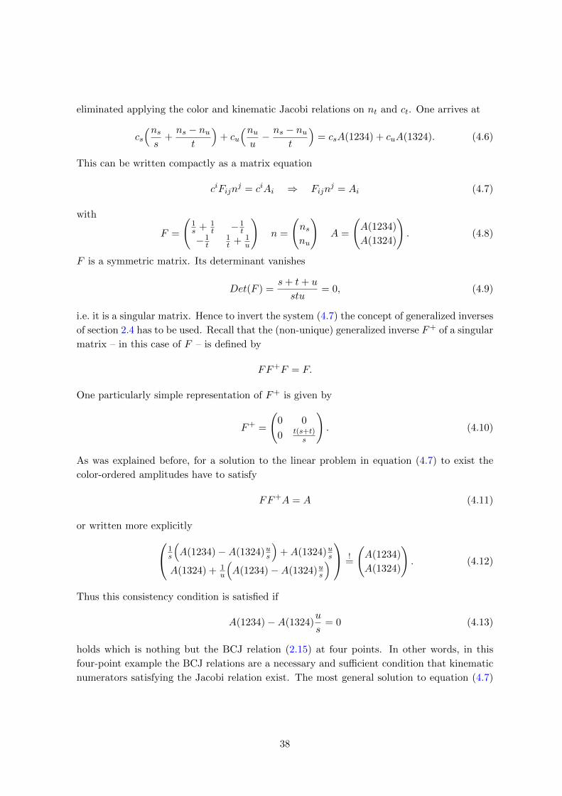
eliminated applying the color and kinematic Jacobi relations on nt and ct. One arrives at
cs
(nss
+ns − nu
t
)+ cu
(nuu− ns − nu
t
)= csA(1234) + cuA(1324). (4.6)
This can be written compactly as a matrix equation
ciFijnj = ciAi ⇒ Fijn
j = Ai (4.7)
with
F =
(1s + 1
t −1t
−1t
1t + 1
u
)n =
(nsnu
)A =
(A(1234)
A(1324)
). (4.8)
F is a symmetric matrix. Its determinant vanishes
Det(F ) =s+ t+ u
stu= 0, (4.9)
i.e. it is a singular matrix. Hence to invert the system (4.7) the concept of generalized inverses
of section 2.4 has to be used. Recall that the (non-unique) generalized inverse F+ of a singular
matrix – in this case of F – is defined by
FF+F = F.
One particularly simple representation of F+ is given by
F+ =
(0 0
0 t(s+t)s
). (4.10)
As was explained before, for a solution to the linear problem in equation (4.7) to exist the
color-ordered amplitudes have to satisfy
FF+A = A (4.11)
or written more explicitly
1s
(A(1234)−A(1324)us
)+A(1324)us
A(1324) + 1u
(A(1234)−A(1324)us
) !
=
(A(1234)
A(1324)
). (4.12)
Thus this consistency condition is satisfied if
A(1234)−A(1324)u
s= 0 (4.13)
holds which is nothing but the BCJ relation (2.15) at four points. In other words, in this
four-point example the BCJ relations are a necessary and sufficient condition that kinematic
numerators satisfying the Jacobi relation exist. The most general solution to equation (4.7)
38
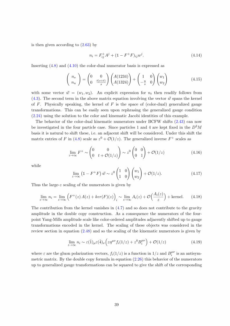
is then given according to (2.63) by
ni = F+ijA
j + (1− F+F )ijwj . (4.14)
Inserting (4.8) and (4.10) the color-dual numerator basis is expressed as
(nsnu
)=
(0 0
0 t(s+t)s
)(A(1234)
A(1324)
)+
(1 0
−us 0
)(w1
w2
)(4.15)
with some vector ~w = (w1, w2). An explicit expression for nt then readily follows from
(4.3). The second term in the above matrix equation involving the vector ~w spans the kernel
of F . Physically speaking, the kernel of F is the space of (color-dual) generalized gauge
transformations. This can be easily seen upon rephrasing the generalized gauge condition
(2.24) using the solution to the color and kinematic Jacobi identities of this example.
The behavior of the color-dual kinematic numerators under BCFW shifts (2.43) can now
be investigated in the four particle case. Since particles 1 and 4 are kept fixed in the D3M
basis it is natural to shift these, i.e. an adjacent shift will be considered. Under this shift the
matrix entries of F in (4.8) scale as z0 +O(1/z). The generalized inverse F+ scales as
limz→∞
F+ ∼(
0 0
0 t+O(1/z)
)∼ z0
(0 0
0 1
)+O(1/z) (4.16)
while
limz→∞
(1− F+F
)~w ∼ z0
(1 0
1 0
)(w1
w2
)+O(1/z). (4.17)
Thus the large-z scaling of the numerators is given by
limz→∞
ni = limz→∞
(F+(z)A(z) + ker(F )(z)
)i∼ lim
z→∞Ai(z) +O
(Ai(z)z
)+ kernel. (4.18)
The contribution from the kernel vanishes in (4.7) and so does not contribute to the gravity
amplitude in the double copy construction. As a consequence the numerators of the four-
point Yang-Mills amplitude scale like color-ordered amplitudes adjacently shifted up to gauge
transformations encoded in the kernel. The scaling of these objects was considered in the
review section in equation (2.48) and so the scaling of the kinematic numerators is given by
limz→∞
ni ∼ ε(1)µε(4)ν
(zηµνfi(1/z) + z0Bµν
i
)+O(1/z) (4.19)
where ε are the gluon polarization vectors, fi(1/z) is a function in 1/z and Bµνi is an antisym-
metric matrix. By the double copy formula in equation (2.26) this behavior of the numerators
up to generalized gauge transformations can be squared to give the shift of the corresponding
39

gravity amplitude in N = 0 SUGRA,
limz→∞
M4 ∼ ε(1)µε(1)κε(4)ν ε(4)λ(zηµνf(1/z) + z0Bµν +O(1/z)
)(zηκλf(1/z) + z0Bκλ +O(1/z)
). (4.20)
Already here one can see the four-point gravity tree amplitude simply scales as two copies
of Yang-Mills amplitudes under a BCFW shift. This reproduces the result by Arkani-Hamed
and Kaplan (2.57) at four points. In the following sections the reasoning will be extended to
all multiplicity at tree level and then to the level of the integrand.
4.1.1. Rephrasing color-kinematics duality as linear algebra
As was seen in the previous section the first step in rewriting color-kinematics duality as a
linear map is to express all color factors and kinematic numerators in a minimal basis. The
basis for the color factors cj will be denoted cj . It is known at tree level that there are
(2n − 5)!! distinct color factors with a minimal basis given in terms of (n − 2)! elements. In
other words any color factor of a tree level trivalent connected graph can be expressed as a
linear combination of the basis elements, i.e. a rectangular matrix Wi j exists for which
ci = Wi j cj j = 1, . . . , (n− 2)! i = 1, . . . , (2n− 5)!!. (4.21)
At tree level, the D3M basis (2.9) is as an example of such a basis. As the kinematic
numerators are assumed to be color-dual the same arguments hold, i.e. the same rectangular
matrix Wi j exists which can be used to express the numerators in terms of a minimal basis
ni = Wi jnj j = 1, . . . , (n− 2)! i = 1, . . . , (2n− 5)!!. (4.22)
This can now be inserted into the BCJ representation (2.16) of the amplitude for both color
as well as kinematic part and leads to
An = gn−2ym
∑
j,k
nj
∑
Γi
WjiWik
si
ck (4.23)
which can be written in the more compact form
An = gn−2ym
∑
j,k
njFjkck (4.24)
after having defined the symmetric (n− 2)!× (n− 2)! matrix F by
Fjk ≡
∑
Γi
Wj iWi k
si
. (4.25)
40
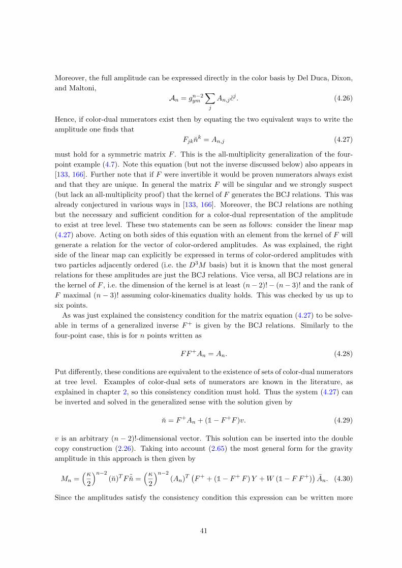
Moreover, the full amplitude can be expressed directly in the color basis by Del Duca, Dixon,
and Maltoni,
An = gn−2ym
∑
j
An,j cj . (4.26)
Hence, if color-dual numerators exist then by equating the two equivalent ways to write the
amplitude one finds that
Fjknk = An,j (4.27)
must hold for a symmetric matrix F . This is the all-multiplicity generalization of the four-
point example (4.7). Note this equation (but not the inverse discussed below) also appears in
[133, 166]. Further note that if F were invertible it would be proven numerators always exist
and that they are unique. In general the matrix F will be singular and we strongly suspect
(but lack an all-multiplicity proof) that the kernel of F generates the BCJ relations. This was
already conjectured in various ways in [133, 166]. Moreover, the BCJ relations are nothing
but the necessary and sufficient condition for a color-dual representation of the amplitude
to exist at tree level. These two statements can be seen as follows: consider the linear map
(4.27) above. Acting on both sides of this equation with an element from the kernel of F will
generate a relation for the vector of color-ordered amplitudes. As was explained, the right
side of the linear map can explicitly be expressed in terms of color-ordered amplitudes with
two particles adjacently ordered (i.e. the D3M basis) but it is known that the most general
relations for these amplitudes are just the BCJ relations. Vice versa, all BCJ relations are in
the kernel of F , i.e. the dimension of the kernel is at least (n− 2)!− (n− 3)! and the rank of
F maximal (n − 3)! assuming color-kinematics duality holds. This was checked by us up to
six points.
As was just explained the consistency condition for the matrix equation (4.27) to be solve-
able in terms of a generalized inverse F+ is given by the BCJ relations. Similarly to the
four-point case, this is for n points written as
FF+An = An. (4.28)
Put differently, these conditions are equivalent to the existence of sets of color-dual numerators
at tree level. Examples of color-dual sets of numerators are known in the literature, as
explained in chapter 2, so this consistency condition must hold. Thus the system (4.27) can
be inverted and solved in the generalized sense with the solution given by
n = F+An + (1− F+F )v. (4.29)
v is an arbitrary (n − 2)!-dimensional vector. This solution can be inserted into the double
copy construction (2.26). Taking into account (2.65) the most general form for the gravity
amplitude in this approach is then given by
Mn =(κ
2
)n−2(n)TF ˜n =
(κ2
)n−2(An)T
(F+ + (1− F+ F )Y +W (1− F F+)
)An. (4.30)
Since the amplitudes satisfy the consistency condition this expression can be written more
41

concisely as
Mn =(κ
2
)n−2(An)T
(F+)An. (4.31)
It is very interesting to note that one particular example of a matrix F+ can be found from
comparing the last equation to the novel realization of the KLT relation in [167]. This also
provides an interesting link of the linear map approach to sting theory via the so-called
momentum kernel of [126].
The previous analysis shows that the matrix F and its generalized inverse F+ encode most
features of color-kinematics duality and do not depend on the specifics of gauge or gravity
theories. In fact F and its generalized inverse arise in any theory built out trivalent vertices
with two Jacobi-satisfying structure constants. Examples of such theories have for instance
been studied in [59, 130] in great detail. A particular class of these theories are scalar field
theories that consist of a single massless scalar and only one trivalent vertex which is made
out of two structure constants satisfying the Jacobi relations. This means that its amplitudes
are given in a cubic form (2.16) with color-dual numerators by construction. In the following
we will call such field theories ‘trivalent scalar theories’.
4.1.2. BCFW shifts of gravity amplitudes constructed by double copy
After having explained how to rephrase color-kinematics duality as a linear map for any
number of external legs at tree level, this can now be used to investigate the BCFW shift
behavior of n-point gravity tree amplitudes. In the following the D3M basis will be used to
fix legs 1 and n, i.e.
∑
Γi
nicisi
=∑
σ∈Pn−2
cσA(1, σ(2), ..., σ(n− 1), n) ≡∑
i
ciAi (4.32)
where Γi runs over all cubic graphs and Pn−2 denotes all permutations of (2, ..., n − 1). As
demonstrated above, this reduces to the linear map
Fijnj = Ai (4.33)
after having solved the color and kinematical Jacobi relations. It can be inverted in terms of
the generalized inverse F+ because the consistency condition is met.
As before the particles fixed in the D3M basis will be subjected to a BCFW shift to obtain
the large-z scaling of the kinematic numerators. As particles 1 and n are adjacent this is an
adjacent shift. F scales as ∼ (z0) under such a BCFW shift as will be seen below. However,
this does not automatically suggest a similar scaling of F+. As a counterexample consider
the following situation with ε→ 0,
A =
(1 0
0 ε
)A+ =
(1 0
0 1ε
). (4.34)
Here, the generalized inverse A+ diverges when ε vanishes.
42
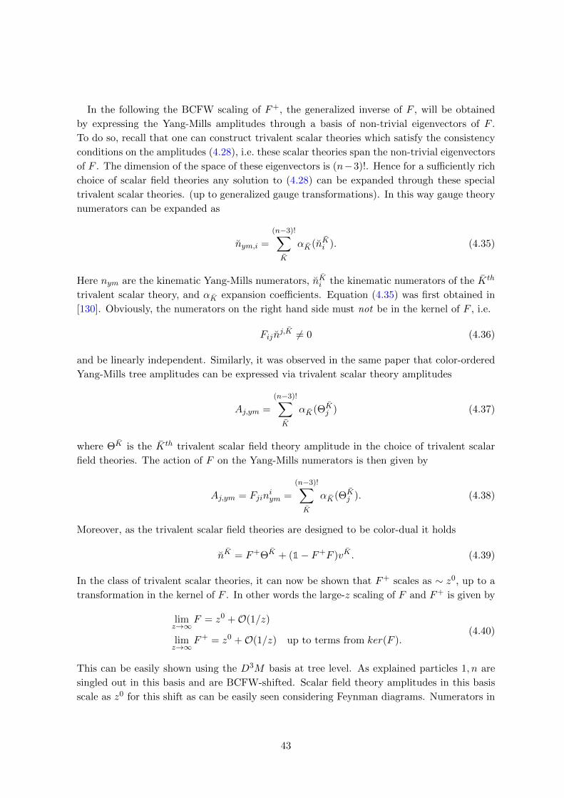
In the following the BCFW scaling of F+, the generalized inverse of F , will be obtained
by expressing the Yang-Mills amplitudes through a basis of non-trivial eigenvectors of F .
To do so, recall that one can construct trivalent scalar theories which satisfy the consistency
conditions on the amplitudes (4.28), i.e. these scalar theories span the non-trivial eigenvectors
of F . The dimension of the space of these eigenvectors is (n−3)!. Hence for a sufficiently rich
choice of scalar field theories any solution to (4.28) can be expanded through these special
trivalent scalar theories. (up to generalized gauge transformations). In this way gauge theory
numerators can be expanded as
nym,i =
(n−3)!∑
K
αK(nKi ). (4.35)
Here nym are the kinematic Yang-Mills numerators, nKi the kinematic numerators of the Kth
trivalent scalar theory, and αK expansion coefficients. Equation (4.35) was first obtained in
[130]. Obviously, the numerators on the right hand side must not be in the kernel of F , i.e.
Fijnj,K 6= 0 (4.36)
and be linearly independent. Similarly, it was observed in the same paper that color-ordered
Yang-Mills tree amplitudes can be expressed via trivalent scalar theory amplitudes
Aj,ym =
(n−3)!∑
K
αK(ΘKj ) (4.37)
where ΘK is the Kth trivalent scalar field theory amplitude in the choice of trivalent scalar
field theories. The action of F on the Yang-Mills numerators is then given by
Aj,ym = Fjiniym =
(n−3)!∑
K
αK(ΘKj ). (4.38)
Moreover, as the trivalent scalar field theories are designed to be color-dual it holds
nK = F+ΘK + (1− F+F )vK . (4.39)
In the class of trivalent scalar theories, it can now be shown that F+ scales as ∼ z0, up to a
transformation in the kernel of F . In other words the large-z scaling of F and F+ is given by
limz→∞
F = z0 +O(1/z)
limz→∞
F+ = z0 +O(1/z) up to terms from ker(F ).(4.40)
This can be easily shown using the D3M basis at tree level. As explained particles 1, n are
singled out in this basis and are BCFW-shifted. Scalar field theory amplitudes in this basis
scale as z0 for this shift as can be easily seen considering Feynman diagrams. Numerators in
43
the trivalent scalar theories manifestly scale as z0, up to generalized gauge transformation.
Consequently by (4.39), F+ has to scale as z0.
Equation (4.38) makes it obvious that the essential information about the large-z scaling
behavior is captured by the coefficient α. As the scalar field theories manifestly scale as z0
the scaling of the coefficients α follows immediately from the BCFW shift of color-adjacent
gluons shown in equation (2.48) as
limz→∞
αK ∼ ε(1)µε(n)ν
(zηµνfK(1/z) + z0Bµν
K
)+O(1/z). (4.41)
Plugging this into (4.35) gives the large-z scaling of kinematic color-dual gauge theory tree
numerators at arbitrary multiplicity as (neglecting the subscript)
limz→∞
ni ∼ limz→∞
ε(1)µε(n)ν
(zηµνf(1/z) + z0Bµν
)i+O(1/z) + kernel (4.42)
up to generalized gauge transformations. In writing the result (4.42) the fact was used that
all kinematic Yang-Mills numerators ni can be expressed as linear combinations of the basis
numerators ni involving only numbers. Strictly speaking this is an upper bound on the scaling:
it could scale better. The result of equation (4.42) is sufficient to obtain the large-z behavior
of the gravity tree amplitude through the double copy construction (2.26).
It follows immediately from the numerators or equivalently from equation (4.30) that the
(extended) Einstein gravity tree level amplitude at arbitrary multiplicity scales as two copies
of Yang-Mills tree amplitudes, i.e. like ∼ 1/z2 (compare (2.57)). While the result itself was
obtained through the background field method already in [150], we explicitly proved here that
color-kinematics duality is the mechanism behind the large suppression in z scaling compared
to the naıve powercounting result ∼ zn−2.
Inclusion of renormalizable matter
Up to now only gluonic matter has been considered. If one includes fermionic and / or scalar
matter in the adjoint representation the same results will be found. To see this note that
the only place where the field content played a role in the arguments was the shift of the
tree-level Yang-Mills amplitudes in the D3M basis. However, as generic fermionic and scalar
matter in the adjoint will obey the same group theoretical structure as the gluons, the D3M
basis also exists for these particles. This and the associated KK relations are explained in
detail in [168]. Futhermore, as was explained in chapter 2, the large-z behavior of amplitudes
for shifts of adjacent gluons at tree level is given by equation (2.48) also when the gluons
couple to scalar and fermionic matter in the adjoint [151]. Thus the entire argument of the
previous sections can be repeated when fermions/scalars in the adjoint are included under the
assumption that color-kinematics holds. The gravity amplitudes constructed by the double
copy construction then simply scale as a double copy of the gauge theory components. In
other words they also scale like (2.57).
44
4.1.3. Improved shift behavior as a consequence of color-kinematics
It was reviewed in chapter 2 that improved BCFW scaling implies additional relations for
color-ordered amplitudes. As we have just seen gravity in fact displays a much improved
scaling behavior with respect to naıve expectations and as was mentioned before this improved
scaling has been used in [149] to derive bonus relations. Naturally, this raises the question
if one can find further scaling improvement in Yang-Mills theories beyond the known 1/z
scaling. Indeed, one can find it and the key in doing so lies in color-kinematics duality
and the observation that gravity is an unordered theory in contrast to color-ordered Yang-
Mills. The results below have also been proven differently based on direct Feynman graph
computations to some extent in [58] and more generally using the BCJ relations in [169, 170].
In the introduction we have already seen how color-ordered amplitudes scale under adjacent
BCFW shifts. Let us first find, based on color-kinematics duality, how these amplitudes scale
under a non-adjacent shift, i.e. a shift were the two shifted particles are not adjacent on
the color trace. To answer this question consider the BCJ representation of a color-ordered
Yang-Mills amplitude
A(1, 2, ..., n) =∑
Γi
nisi. (4.43)
with the sum running over all cubic color-ordered graphs. In a non-adjacent shift the two
shifted legs will never meet on a cubic vertex so that there will always be at least one hard
propagator connecting the vertices to which the shifted particles are attached. As the numer-
ators can be expressed via (4.42) which scales homogeneously in z, a non-adjacent shift gives
thus immediately one power of suppression in z with respect to the adjacent one. One finds
for the non-adjacent shift of a color-ordered amplitude
limz→∞
A(1, ..., i, ..., j, ..., n) ∼ ε(i)µε(j)ν(z0ηµνf(1/z) +
1
zBµν
)+O(1/z2). (4.44)
In fact, as will be seen in chapter 5 explicitly also the Yang-Mills integrand scales like this
for a non-adjacent shift. This mirrors the results for adjacent shifts where it is known that
the Yang-Mills integrand scales like the tree amplitude under an adjacent shift. This was
explained earlier in chapter 2.
Permutation sums
To generalize the above result on improved shift behavior focus first on permutation sums.
Consider again the BCJ representation of a color-ordered Yang-Mills amplitude
A(1, 2, ..., n) =∑
Γi
nisi.
45
BCFW-shift now any two particles, say i and j, and study the permutation sum of all particles
in between, i.e.
∑
P{i+1,...,j−1}
A(1, 2, ..., i, ..., j, ..., n) ∼∑
P{i+1,...,j−1}
∑
Γi
nisi. (4.45)
Each of the diagrams on the right hand side will have a unique hard line, i.e. a unique path
along which the z-dependence flows. The lines attaching to the hard line will be one-leg
off-shell currents Jµ(m) with m on-shell legs. However, as can be shown permutation sums
of these currents vanish ∑
σ∈P{1,...,k}
Jµ(σ(1), ..., σ(k)) = 0 (4.46)
the only way they can contribute is when they only contain one leg, i.e. when the permuted
particles connect to the hard line directly. Each additional particle will give a 1/z suppression
due to the hard propagator. With the large-z numerator scaling found in the previous section
(4.42) one finds
limz→∞
∑
P{i+1,...,j−1}
A(1, 2, ..., i, ..., j, ..., n) ∼ 1
zkεµ(i)εν(j)
(zηµνf(1/z) + z0Bµν +O(1/z)
)
(4.47)
with k = j − i − 1. If the shifted particles are adjacent one has to impose k → k − 1 as
there is one hard propagator less. For one permuted particle, i.e. a non-adjacent shift, one
immediately recovers (4.44).
Cyclic sums
A second mechanism to find improved BCFW scaling behavior is cyclic sums. The key
observation here is that n-gluon currents obey a so-called sub-cyclic identity
∑
σ∈Z{1,...,n}
Jµ(σ) = 0. (4.48)
The sum ranges over all cyclic permutations of the n on-shell gluons on the current. This
again implies improvements in the large-z scaling for the color-ordered amplitude. As before
consider the color-ordered version of a BCJ representation and BCFW shift any two particles
i and j. Then the cyclic sum over the particles in between the shifted legs will give
limz→∞
∑
Z{i+1,...,j−1}
A(1, 2, ..., i, ..., j, ..., n) ∼ 1
zkεµ(i)εν(j)
(zηµνf(1/z) + z0Bµν +O(1/z)
).
(4.49)
with k = 2 for non-adjacent shifts and k = 1 for adjacent shifts. This can again be easily
seen: consider first an adjacent shift. In terms of diagrams the leading one will have a cubic
vertex with the two shifted legs directly attached to it. The unshifted leg on this vertex will
contract into a current involving all the other particles; but as was just explained above a
cyclic sum on such a current will vanish so that this diagram will not contribute and the
46
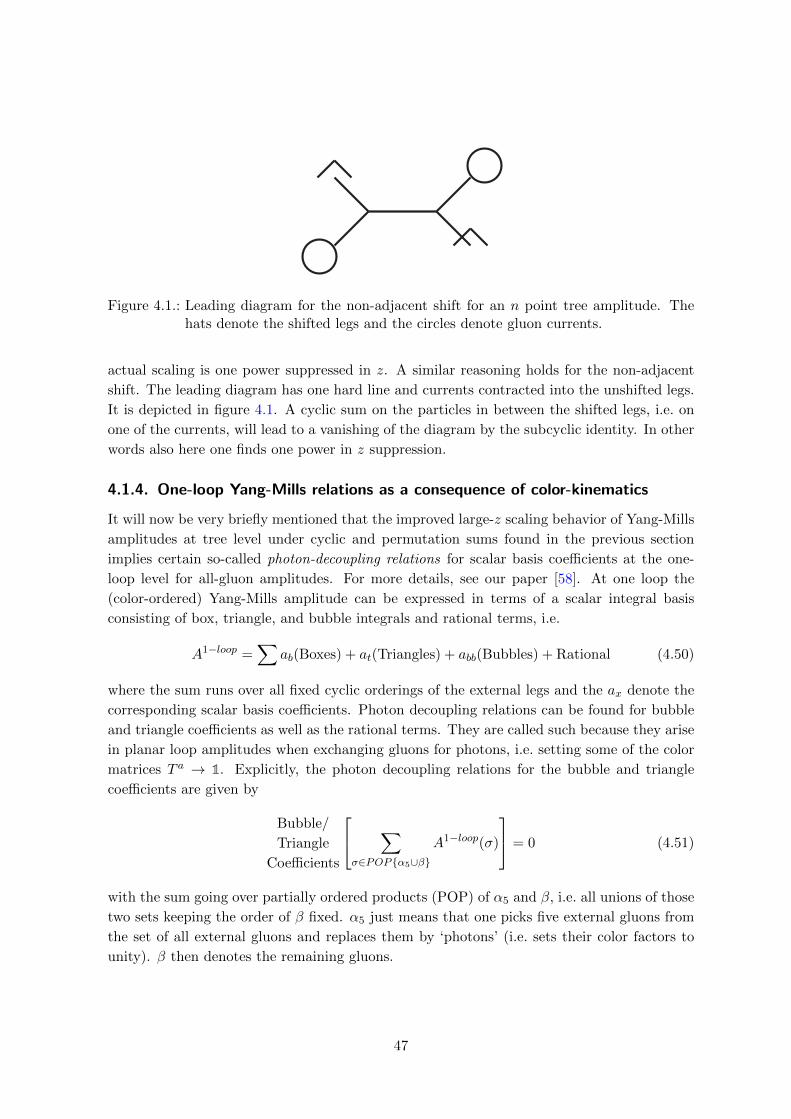
Figure 4.1.: Leading diagram for the non-adjacent shift for an n point tree amplitude. Thehats denote the shifted legs and the circles denote gluon currents.
actual scaling is one power suppressed in z. A similar reasoning holds for the non-adjacent
shift. The leading diagram has one hard line and currents contracted into the unshifted legs.
It is depicted in figure 4.1. A cyclic sum on the particles in between the shifted legs, i.e. on
one of the currents, will lead to a vanishing of the diagram by the subcyclic identity. In other
words also here one finds one power in z suppression.
4.1.4. One-loop Yang-Mills relations as a consequence of color-kinematics
It will now be very briefly mentioned that the improved large-z scaling behavior of Yang-Mills
amplitudes at tree level under cyclic and permutation sums found in the previous section
implies certain so-called photon-decoupling relations for scalar basis coefficients at the one-
loop level for all-gluon amplitudes. For more details, see our paper [58]. At one loop the
(color-ordered) Yang-Mills amplitude can be expressed in terms of a scalar integral basis
consisting of box, triangle, and bubble integrals and rational terms, i.e.
A1−loop =∑
ab(Boxes) + at(Triangles) + abb(Bubbles) + Rational (4.50)
where the sum runs over all fixed cyclic orderings of the external legs and the ax denote the
corresponding scalar basis coefficients. Photon decoupling relations can be found for bubble
and triangle coefficients as well as the rational terms. They are called such because they arise
in planar loop amplitudes when exchanging gluons for photons, i.e. setting some of the color
matrices T a → 1. Explicitly, the photon decoupling relations for the bubble and triangle
coefficients are given by
Bubble/
Triangle
Coefficients
∑
σ∈POP{α5∪β}
A1−loop(σ)
= 0 (4.51)
with the sum going over partially ordered products (POP) of α5 and β, i.e. all unions of those
two sets keeping the order of β fixed. α5 just means that one picks five external gluons from
the set of all external gluons and replaces them by ‘photons’ (i.e. sets their color factors to
unity). β then denotes the remaining gluons.
47

For the rational terms the decoupling relation reads
Rational
∑
σ∈POP{α3∪β}
A1−loop(σ)
= 0. (4.52)
The sum is over again partially ordered products but this time the set α contains only three
external gluons. The relations can be crosschecked nicely numerically [171].
While all of the above decoupling relations are independent of the helicities of the involved
gluons, the relations (4.52) had first been found for a specific choice of helicity [123, 124].
For a detailed proof of the above relations, the reader is again referred to our paper [58].
The key point in proving them, however, is that scalar basis coefficients can be expressed via
generalized unitarity as certain products of Yang-Mills tree amplitudes expanded in a certain
large momentum limit. Following this idea, the results from the previous section at tree level
for improved large BCFW shifts can be used to show that the relations are indeed true. As
the improved large-z scaling at tree level is nothing but a consequence of color-kinematics
duality, in fact also these one-loop results can by extension be regarded as arising due the
duality.
Note further that also certain rational all-plus and one-minus one-loop relations first found
in [123] can be proven along the same lines. The interested reader is once more referred to
[58] for explicit details of the large-momentum-shift based proof. In addition, these relations
can be directly seen as a consequence of color-kinematics duality at one-loop. In this way the
all-plus relations have been verified explicitly based on color-kinematics duality in our paper
[101].
4.2. BCFW shifts of gravity integrands from gauge theory
In this section the results on BCFW scaling of Einstein gravity tree amplitudes obtained
through color-kinematics duality will be extended to the integrand level. It will be argued
that basically all the steps of the tree-level derivation can be repeated up to several subtleties
and assumptions that will be made precise below. The assumptions that will be needed in
the following are:
(i) Color-dual numerators exist on the integrand level and any consistency conditions on
the Yang-Mills integrands are fulfilled.
(ii) Generalized gauge transformations do not influence the double copy relations.
(iii) Trivalent scalar theories span the set of integrands which satisfy the consistency condi-
tions.
(iv) In the chosen color-basis coefficients of the integrand for trivalent scalar theories scale
the same or worse (higher powers in z) compared to the corresponding coefficient for
the Yang-Mills integrand.
48
4.2.1. BCFW shifts of kinematic numerators using generalized inverses
As was explained in the review chapter at the beginning of this thesis, the integrand of a
l-loop n-point Yang Mills amplitude can be written using cubic graphs only through equation
(2.27)
Al−loopn = gn−2+2lym
∫ l∏
j=1
dDLj∑
Γi
1
Si
nicisi
.
The color-factors ci obey a set of Jacobi relations and it will be assumed that a set of color-
dual kinematic numerators ni can be found. Just as in the tree level case, the Jacobi relations
can be solved and so a minimal basis for the color factors and numerators denoted by c, n of
dimension h can be constructed. At one loop an explicit realization of such a basis is known:
the basis used by D3M in equation (2.12) with h = (n−1)!/2. The cubic representation above
can be rewritten upon insertion of the basis color factors and numerators (again following the
tree level example closely and neglecting all coupling constants in the following) as
Al−loopn ∼∫ l∏
j=1
dDLj∑
Γi
1
Si
nicisi∼ ck
∫ l∏
j=1
dDLjFkmnm (4.53)
where k and m run from 1 to h and F is a matrix whose entries are sums over products of
scalar propagators and symmetry factors. It can be easily seen that F is not unique as it
depends column by column on the definition of loop momentum and this need to be taken
into account carefully when summing up the scalar propagators.
The full l-loop amplitude can also be expressed in a higher-loop generalization of the D3M
basis directly, i.e. in a l-loop minimal-color basis symbolically given by
Al−loopn = ck∫ l∏
j=1
dDLj IYMk . (4.54)
Note again that a precise formulation of such a basis is not yet known beyond one loop;
however, its existence is likely and various results indicate that it can be constructed from a
subset of color-ordered integrands only [116–118].
In contrast to tree level one cannot extract the equation
IYMj = Fjmnm (does not hold) (4.55)
at the level of the integrand by equating (4.53) and (4.54). The point here is to note that
one can always add terms to the loop integral that integrate to zero. In other words: the
numerators live in the space of vectors of functions of external and loop momenta,
n ∼
f1(pi, Li)
f2(pi, Li)
. . .
(4.56)
49
while the integrands live in the space of vectors of functions of external and loop momenta,
identified up to terms which integrate to zero. That is,
I ∼
f1(pi, Li)
f2(pi, Li)
. . .
(4.57)
where two functions f and g are equivalent, f ∼ g, if
∫ l∏
j=1
dDLj f =
∫ l∏
j=1
dDLj g (4.58)
holds. Therefore the space of integrands is smaller than the space of numerators. As a linear
map the matrix F therefore can have a non-trivial kernel.
To keep the possible ambiguity as little as possible the routing of the loop momenta for
numerators and the integrand will be taken to be identical. For a BCFW shift this means
that the hard line will be chosen such that it is the path minimizing the distance between the
shifted legs. In general the equation to solve (using the notation of section 2.4) is
Fjmnm ∼ IYMj (4.59)
or equivalently in the space on which the numerators live
Fjmnm = IYMj + Ivanishj (4.60)
with Ivanish integrating to zero. For a solution to equation (4.59) to exist there could be
consistency conditions if there are left null eigenvectors of Fn. Note that ‘null’ in this sentence
is up to terms which vanish after integration. At one loop we strongly suspect the relation
we found in [57] is the full set of consistency conditions for local numerators. Explicitly, this
one-loop relation is given (up to terms integrating to zero) by
n−1∑
i=1
kα ·(L+ kn−1 +
i−1∑
j=1
kj
)I(1, ..., i− 1, α, i, ....n− 1) ∼ 0 (4.61)
where I(1, ...) is the color-ordered one-loop integrand and L the loop momentum defined such
that the propagator after particle n − 1 is 1/(L + kn−1)2 (momenta taken incoming). The
above relation is the one-loop integrand generalization of the tree-level BCJ relations. Having
the foregoing discussion of large-z shifts in mind, this relation is in fact due to the improved
scaling of gauge theory integrands under non-adjacent BCFW shifts. It was argued in [57, 58]
that similar relations might exist at higher loops. Also here the argument was given on the
basis of the improved behavior of Yang-Mills integrands under non-adjacent BCFW shifts to
all loop orders (see chapter 5).
Assuming that color-dual numerators exist is equivalent to assuming that all consistency
condition on the linear map are satisfied as was seen already at tree level in equation (4.28).
50
So if this is true the numerators at loop level can be obtained by means of (2.71) as
n = F+(IYM + Ivanish) + kerF. (4.62)
At tree level the kernel of F gave rise to generalized gauge transformations. It was argued
that these do not affect the squaring relation. However, at the integrand level the same is
not necessarily true anymore as discussed above in section 2.2. As was also discussed in
that section this is a problem inherent to the color-kinematics duality. We will assume in
the following that this issue will not have an impact on the outcome of the double copy
construction for the integrand in the following analysis.
Further assume that the non-trivial eigenvectors of F are spanned by the previously in-
troduced trivalent scalar theories. Put differently, the space of solutions to the consistency
conditions at loop level is spanned by this class of theories. At one loop it is certainly true
that trivalent scalar theories as well as Yang-Mills theories satisfy the relation (4.61). Thus
the assumption states that the left-side kernel of the map F
left kerF = {mj |miFijnj = 0} (4.63)
is the same set for numerators from the trivalent scalar theories as well as Yang-Mills theory.
Further evidence for this assumption can also be provided by estimates on the dimension of
the kernel in both cases in the large-z limit: this is basically the observation that the number
of independent integrands at n points under BCJ-like relations (4.61) is equal to the number
of independent integrands under KK relations for n − 1 particles. This number is the same
for trivalent scalar theories and Yang-Mills theory.
With this assumption the scaling of the generalized inverse F+ up to gauge transformations
can be obtained similarly to the tree level by writing the Yang-Mills numerators in a scalar
numerator basis
ni =∑
K
αK nKi (4.64)
where the trivalent scalar theory numerators nKi should not be in the kernel of F , i.e.
FjinKi 6= 0. (4.65)
Also the numerators are taken to be linearly independent. Unbarred indices run from 1 to
h with h the number of color-ordered integrands independent under loop-level KK relations.
Barred indices range from 1 to the number of independent color-ordered integrands under the
consistency conditions, i.e. the integrand level analogs of the tree level BCJ relations. In this
way the Yang-Mills integrand can be expanded as
(I + Ivanish)i =∑
J
αJΘJi . (4.66)
ΘJi is the integrand of the Jth trivalent scalar field theory. As before, the action of any
51
generalized inverse F+ on ΘJi can be inferred as
nK = F+ΘK + kerF. (4.67)
Here the left hand side scales as z0 up to a generalized gauge transformation under a BCFW
shift. In general the right hand side can be more complicated. Consider one loop: in the
D3M basis a shift of two legs will be either adjacent or non-adjacent since only one leg is
kept fixed. F will still scale like ∼ (z0) in this case whereas the scaling of F+ can be found
by powercounting from the above equation roughly as
F+Θ ∼(∼ z0 ∼ z1
∼ z0 ∼ z1
)(∼ z0
∼ z−1
)(4.68)
up to a generalized gauge transformation at one loop.
At one loop the color-dual Yang-Mills numerators are then given by
n(1−loop)ym = F+I(1−loop)
ym ∼ ε(1)µε(n)ν
(zηµνf(1/z) + z0Bµν
)+O(1/z) + kernel (4.69)
from the results for adjacent (2.48) and non-adjacent shifts (4.44) for Yang-Mills loop-level
integrands. Note that this result is up to terms which integrate to zero. If they displayed a
worse scaling behavior they would have to satisfy the consistency conditions themselves, i.e.
they are generalized gauge transformations.
The extension of this argument to higher loops goes through under an additional assump-
tion: if one of the coefficients in the scalar basis integrand vector shows improved BCFW
scaling behavior, the corresponding gauge theory coefficients must do so as well. Generically,
as was already seen above, these coefficients are expected to either involve adjacent or non-
adjacent shifts for which the shift behavior is known. This assumption is quite sensible in
view of the already mentioned results of [116–118] who conjectured a basis for up to six-point
integrands which is simply a subset of the full set of color-ordered integrands.
Hence up to the assumptions and generalized gauge transformations the large-z scaling of
the color-dual numerators in Yang-Mills is to all loop orders is given by
limz→∞
nk ∼ ε(1)µε(n)ν
(zηµνf(1/z) + z0Bµν
)k
+O(1/z) + kernel. (4.70)
4.2.2. BCFW shifts of gravity integrands constructed by double copy
The double copy construction at loop level can also be rephrased using linear maps as follows
from considering (2.26). One finds (suppressing the coupling constant)
M l−loopn ∼
∫ l∏
j=1
dDLj∑
Γi
1
Si
ninisi∼∫ l∏
j=1
dDLj ˜niFijnj (4.71)
where ˜n and n are sets of kinematic basis numerators from two copies of gauge theory. The
large-z behavior of the numerators at any loop order (4.70) and of F have been found in the
52
previous sections. Hence for the shift of particles 1 and n the large-z scaling of the n-graviton
N = 0 gravity integrand In is given by a double copy of equation (4.70)
limz→∞
In ∼ ε(1)µε(n)ν ε(1)µε(n)ν
(z2ηµν ηµνf(1/z) + z(ηµνBµν +Bµν ηµν)+
z0(BµνBµν) +1
z(BµνBµν)
)+O(1/z2)
(4.72)
up to the assumptions made precise above and especially assuming that generalized gauge
transformation do not interfere with the double copy construction. Note that this result is
structurally the same as the tree level result (2.57). It displays quite drastic cancellations in
z with respect to naıve expectations: based on powercounting Feynman graphs one would
have guessed a scaling given by ∼ zn−2+2l but as is obvious from the above formula the
largest power in z is quadratic and moreover completely independent of the loop order l. As
in the tree level case the mechanism behind this improvement is the assumed existence of
color-kinematic duality.
Also note that the result (4.72) for the N = 0 integrand is the same including scalars or
fermions in the adjoint. This follows from the argument for adding matter at tree level in
section 4.1.2 based on results in [58, 145].
4.3. Estimates on UV behavior from color-kinematics duality
Ultimately, the goal in the study of cancellations in gravity theories is to better understand
their UV behavior. To this end the same linear map approach can be used that was already
employed in the study of cancellations in BCFW shifts through powercounting. In this context
it is also interesting to note that the relation between the large BCFW behavior and the UV
degree of divergence goes deeper than powercounting. They are closely related in that the
good behavior of gravity tree amplitudes under BCFW shifts gives rise to the absence of scalar
triangle integrals at one loop in N = 8 supergravity as was studied in [14] (see also [172]). In
view of the analysis above this result is nothing but a consequence of color-kinematics duality.
This result is in fact valid for the integrand at any loop order by unitarity. Consequently,
there is no triangle divergence in N = 4 super Yang-Mills nor N = 8 supergravity.
In the following it will be argued that color-kinematics duality leads to improved power-
counting of gravity integrands up to assumptions (which are similar to those encountered in
the previous section)
• Color-dual numerators exist and any consistency conditions on the Yang-Mills inte-
grands are fulfilled.
• Generalized gauge transformations do not influence the double copy relations.
• Trivalent scalar theories span the set of integrands which satisfy the consistency condi-
tions.
• If there is a vanishing integrand, potential worse scaling behavior of this integrand can
be absorbed into a generalized gauge transformation.
53
• If the integrands of the trivalent scalar theories to be considered show improvement over
the leading behavior the same holds for the gauge theory integrands.
The UV degree of divergence will be studied in the limit of large loop momenta, i.e.
Li →∞ ∀i. (4.73)
Hence the analysis is restricted to the overall degree of divergence of diagrams. Sub- and
overlapping divergences will be ignored. Note that even if powercounting gives a possible
divergence it could still integrate to zero or vanish in the sum of all graphs.
As integrands from Yang-Mills will be the input for the double copy construction it is
instructive to briefly review the UV properties of pure Yang-Mills and its maximally super-
symmetric cousin. Pure Yang-Mills theory diverges logarithmically in four dimensions at
one loop, whereas maximally supersymmetric Yang-Mills diverges at the same loop order in
D = 8. This can nicely be seen in the decomposition of the gauge theory integrands coupled
to massless matter in terms of a scalar integral basis consisting of boxes, triangles, bubbles:
N = 4 at one loop can be written in terms of boxes only (diverging in D = 8). Expressing
pure Yang-Mills theory in the scalar basis involves all the aforementioned topologies with the
UV divergence in D = 4 encoded in the bubble diagrams. Note as an aside that the sum over
bubble coefficients is related to tree level amplitudes (see [14] and especially [173]).
The degree of divergence of pure Yang-Mills can also be seen using gauge invariance ar-
guments: naıve powercounting of Feynman graphs suggests a quadratic divergence in two
dimensions. However, in dimensional regularization this divergence is absent as can be seen
from the background field method: the functional form of the two-point correlator of two
(background) gauge fields which contains the two dimensional divergence has to be propor-
tional to
〈AµAν〉 ∼ gµνp2 + pµpν (4.74)
by background field gauge invariance. The two-dimensional divergence would appear with
the first term, while the second term cannot arise with a two-dimensional divergence. Hence
by gauge invariance the two-dimensional divergences must vanish and consequently generic
Yang-Mills theories are logarithmically divergent in four dimensions. Sometimes this is also
stated as ‘gauge invariance softens divergences’.
Starting at two loops one finds [174, 175] that maximally supersymmetric Yang-Mills di-
verges logarithmically in
Dc =6
l+ 4, l ≥ 2 (4.75)
dimensions with l the loop order. This behavior has been explicitly verified up to and including
five loops [54] for the planar and non-planar sector and to six loops in the planar sector in
[176]. The critical dimension in maximally supersymmetric Yang-Mills theory translates into
a powercount for the integrand of N = 4 Yang-Mills as
∫dDlL
(L2)l−2
(L2)3l+1(4.76)
54
at loop order l. The number of propagator powers is that of a four-point amplitude with the
maximal number of loop propagators.
Let us now extend and adapt the analysis of large BCFW shifts using color-kinematics
duality to the limit of large loop momenta. With the above assumptions the behavior of F+
can be studied via trivalent scalar theories in this limit. The numerators of these theories do
not depend on loop momenta. The scaling of F+ up to generalized gauge transformation is
given by
nK = F+(Itrivalent,K) + kerF (4.77)
for the K-th trivalent scalar theory. The right hand side of this equation, i.e. the integrand
basis I, denotes as usual the basis which is minimal under KK relations. This basis was
already argued to exist beyond one-loop in the previous sections and is most likely a subset
of all color-ordered integrands. In general, some of these basis elements will be non-planar
while others are planar. The former ones are better UV behaved than the latter ones. This
is a consequence of renormalizability as the overall UV degree is related to the planar, i.e.
single trace, terms because the UV divergent terms must be such that they can be absorbed
into a counterterm proportional to the Yang-Mills action. More specifically, the must be
proportional to tree level amplitudes.
So generically, the integrand vector I might not scale homogeneously for large loop mo-
menta. A similar situation has already been encountered before in equation (4.68) for large
BCFW shifts. Say, it partly scales as (L2)−δ1 and partly (L2)−δ2 . In this case the generalized
inverse F+ scales schematically as
if I ∼(
(L2)−δ1
(L2)−δ2
)then F+ ∼
((L2)δ1 (L2)δ2
). (4.78)
Of course, if the integrand scales homogeneously, i.e. all δ are the same, then F+ simply
scales inversely. The scaling of F+ is as before up to generalized gauge transformations
and it determines the powercounting behavior of the color-dual gauge theory numerators by
expanding them in the trivalent scalar theory basis.
The following step is a crucial, non-trivial one: which trivalent graphs should be included
in equation (2.27)? In other words, which graphs have non-vanishing numerators? For N = 4
Yang-Mills it is natural to exclude triangle graphs. One the one hand this shrinks the set of
trivalent graphs and on the other it simplifies the Jacobi identities enormously. The solution
to the set of numerator Jacobi relations will in this way be smaller than the solution for color
Jacobi relations. The former statement can be phrased as a matrix equation
nj = NjM nM . (4.79)
j ranges over all elements of the set of solutions to the color Jacobi relations and usually
j >> M . In fact, it is well known from many examples, see e.g. [134], that all color-dual
numerators can be expressed in terms of just one or two ‘master’ numerators (that of course
than means that all graphs can be expressed in terms of one or two ‘master’ graphs).
55

Powercounting at one loop
Having discussed the assumptions at the beginning of this section and having the discussion
of the last section in mind, the gravity integrand (4.71) can be written as
M l−loopn ∼
∫ l∏
j=1
dDLj∑
Γi
niFij ˜nj ∼
∫ l∏
j=1
dDLj IiF+,ijIj . (4.80)
At one loop for N = 4 Yang-Mills theory, excluding triangle graphs gives a large loop mo-
mentum scaling of the generalized inverse as
F+ ∼ (L2)4 N = 4, 1 loop (4.81)
from the trivalent scalar theories (4.77). This is easy to see because all the entries in the
integrand vector in the D3M basis contain at least a box. This gives for the Yang-Mills
numerators, taking into account that the Yang-Mills integrand also scales like boxes,
nym ∼ F+Iym ∼ (L2)0 N = 4, 1 loop. (4.82)
For less-supersymmetric Yang-Mills one finds due to bubble graphs
F+ ∼ (L2)2 N < 4, 1 loop (4.83)
which implies
nym ∼ (L2)0 N < 4, 1 loop. (4.84)
Inserting these results into the double copy construction (4.80) nicely reproduces the known
critical dimensions from the literature under the assumptions listed above and up to general-
ized gauge transformations. More specifically, one finds that the critical dimension of N = 0
supergravity is D = 4 while for N = 8 it is D = 8 at one loop. Of course, this analysis does
not check whether the critical dimensions are really saturated. In addition, the double copy
formula also implies the no-triangle property of N = 8 in this way as a consequence of the
absence of triangles in N = 4 super Yang-Mills.
Powercounting at higher loops
At one loop it was more less straightforward which graphs topologies to include in the duality.
However, at higher loops this is not so trivial anymore and in general the set of graphs will
have a large effect on the scaling of the generalized inverse F+. Consider again N = 4 super
Yang-Mill at four points. For the case of trivalent graphs having the maximal possible number
of loop propagators one finds from the trivalent scalar theories
F+ ∼ (L2)3l+1 N = 4,max # loop propagators (4.85)
56
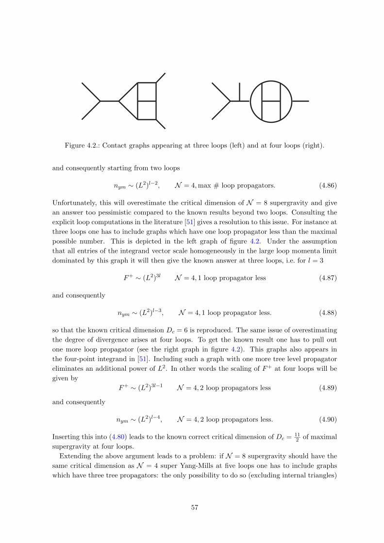
Figure 4.2.: Contact graphs appearing at three loops (left) and at four loops (right).
and consequently starting from two loops
nym ∼ (L2)l−2, N = 4,max # loop propagators. (4.86)
Unfortunately, this will overestimate the critical dimension of N = 8 supergravity and give
an answer too pessimistic compared to the known results beyond two loops. Consulting the
explicit loop computations in the literature [51] gives a resolution to this issue. For instance at
three loops one has to include graphs which have one loop propagator less than the maximal
possible number. This is depicted in the left graph of figure 4.2. Under the assumption
that all entries of the integrand vector scale homogeneously in the large loop momenta limit
dominated by this graph it will then give the known answer at three loops, i.e. for l = 3
F+ ∼ (L2)3l N = 4, 1 loop propagator less (4.87)
and consequently
nym ∼ (L2)l−3, N = 4, 1 loop propagator less. (4.88)
so that the known critical dimension Dc = 6 is reproduced. The same issue of overestimating
the degree of divergence arises at four loops. To get the known result one has to pull out
one more loop propagator (see the right graph in figure 4.2). This graphs also appears in
the four-point integrand in [51]. Including such a graph with one more tree level propagator
eliminates an additional power of L2. In other words the scaling of F+ at four loops will be
given by
F+ ∼ (L2)3l−1 N = 4, 2 loop propagators less (4.89)
and consequently
nym ∼ (L2)l−4, N = 4, 2 loop propagators less. (4.90)
Inserting this into (4.80) leads to the known correct critical dimension of Dc = 112 of maximal
supergravity at four loops.
Extending the above argument leads to a problem: if N = 8 supergravity should have the
same critical dimension as N = 4 super Yang-Mills at five loops one has to include graphs
which have three tree propagators: the only possibility to do so (excluding internal triangles)
57
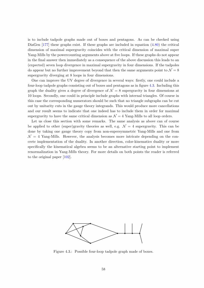
is to include tadpole graphs made out of boxes and pentagons. As can be checked using
DiaGen [177] these graphs exist. If these graphs are included in equation (4.80) the critical
dimension of maximal supergravity coincides with the critical dimension of maximal super
Yang-Mills by the powercounting arguments above at five loops. If these graphs do not appear
in the final answer then immediately as a consequence of the above discussion this leads to an
(expected) seven loop divergence in maximal supergravity in four dimensions. If the tadpoles
do appear but no further improvement beyond that then the same arguments point to N = 8
supergravity diverging at 8 loops in four dimensions.
One can improve the UV degree of divergence in several ways: firstly, one could include a
four-loop tadpole graphs consisting out of boxes and pentagons as in figure 4.3. Including this
graph the duality gives a degree of divergence of N = 8 supergravity in four dimensions at
10 loops. Secondly, one could in principle include graphs with internal triangles. Of course in
this case the corresponding numerators should be such that no triangle subgraphs can be cut
out by unitarity cuts in the gauge theory integrands. This would produce more cancellations
and our result seems to indicate that one indeed has to include them in order for maximal
supergravity to have the same critical dimension as N = 4 Yang-Mills to all loop orders.
Let us close this section with some remarks. The same analysis as above can of course
be applied to other (super)gravity theories as well, e.g. N = 4 supergravity. This can be
done by taking one gauge theory copy from non-supersymmetric Yang-Mills and one from
N = 4 Yang-Mills. However, the analysis becomes more intricate depending on the con-
crete implementation of the duality. In another direction, color-kinematics duality or more
specifically the kinematical algebra seems to be an alternative starting point to implement
renormalization in Yang-Mills theory. For more details on both points the reader is referred
to the original paper [102].
Figure 4.3.: Possible four-loop tadpole graph made of boxes.
58
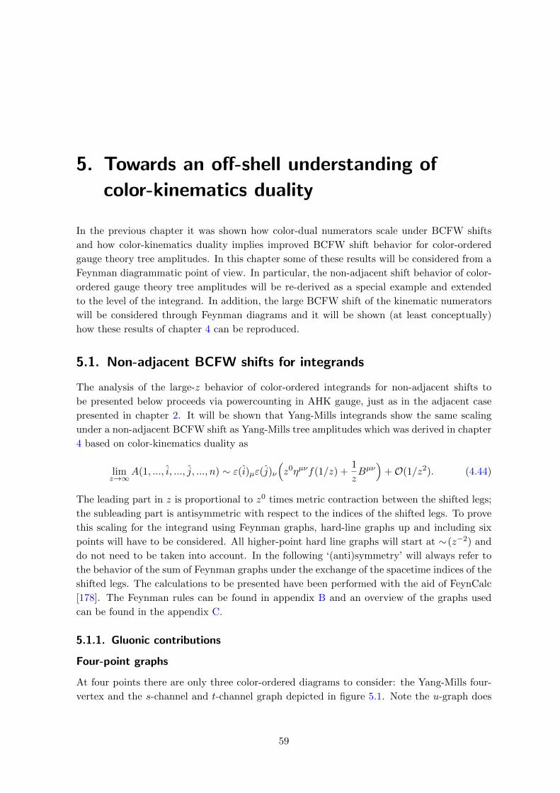
5. Towards an off-shell understanding of
color-kinematics duality
In the previous chapter it was shown how color-dual numerators scale under BCFW shifts
and how color-kinematics duality implies improved BCFW shift behavior for color-ordered
gauge theory tree amplitudes. In this chapter some of these results will be considered from a
Feynman diagrammatic point of view. In particular, the non-adjacent shift behavior of color-
ordered gauge theory tree amplitudes will be re-derived as a special example and extended
to the level of the integrand. In addition, the large BCFW shift of the kinematic numerators
will be considered through Feynman diagrams and it will be shown (at least conceptually)
how these results of chapter 4 can be reproduced.
5.1. Non-adjacent BCFW shifts for integrands
The analysis of the large-z behavior of color-ordered integrands for non-adjacent shifts to
be presented below proceeds via powercounting in AHK gauge, just as in the adjacent case
presented in chapter 2. It will be shown that Yang-Mills integrands show the same scaling
under a non-adjacent BCFW shift as Yang-Mills tree amplitudes which was derived in chapter
4 based on color-kinematics duality as
limz→∞
A(1, ..., i, ..., j, ..., n) ∼ ε(i)µε(j)ν(z0ηµνf(1/z) +
1
zBµν
)+O(1/z2). (4.44)
The leading part in z is proportional to z0 times metric contraction between the shifted legs;
the subleading part is antisymmetric with respect to the indices of the shifted legs. To prove
this scaling for the integrand using Feynman graphs, hard-line graphs up and including six
points will have to be considered. All higher-point hard line graphs will start at ∼(z−2) and
do not need to be taken into account. In the following ‘(anti)symmetry’ will always refer to
the behavior of the sum of Feynman graphs under the exchange of the spacetime indices of the
shifted legs. The calculations to be presented have been performed with the aid of FeynCalc
[178]. The Feynman rules can be found in appendix B and an overview of the graphs used
can be found in the appendix C.
5.1.1. Gluonic contributions
Four-point graphs
At four points there are only three color-ordered diagrams to consider: the Yang-Mills four-
vertex and the s-channel and t-channel graph depicted in figure 5.1. Note the u-graph does
59
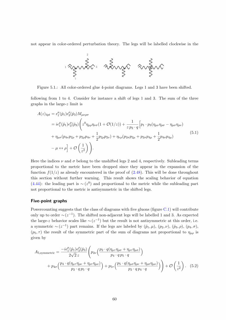
not appear in color-ordered perturbation theory. The legs will be labelled clockwise in the
1
2
3
4
Figure 5.1.: All color-ordered glue 4-point diagrams. Legs 1 and 3 have been shifted.
following from 1 to 4. Consider for instance a shift of legs 1 and 3. The sum of the three
graphs in the large-z limit is
A(z)4pt = εµ1 (p1)ερ3(p3)Mµνρσ
= iεµ1 (p1)ερ3(p3)
(z0ηµρηνσ(1 +O(1/z)) +
1
z p2 · q[p1 · p3(ηµνηρσ − ηµσηρν)
+ ηµσ(p4νp2ρ + p2ρp4ν +1
2p2ρp2ν) + ηνρ(p2σp2µ + p2σp4µ +
1
2p4σp4µ)
− µ↔ ρ]
+O(
1
z2
)).
(5.1)
Here the indices ν and σ belong to the unshifted legs 2 and 4, respectively. Subleading terms
proportional to the metric have been dropped since they appear in the expansion of the
function f(1/z) as already encountered in the proof of (2.48). This will be done throughout
this section without further warning. This result shows the scaling behavior of equation
(4.44): the leading part is ∼ (z0) and proportional to the metric while the subleading part
not proportional to the metric is antisymmetric in the shifted legs.
Five-point graphs
Powercounting suggests that the class of diagrams with five gluons (figure C.1) will contribute
only up to order ∼(z−1). The shifted non-adjacent legs will be labelled 1 and 3. As expected
the large-z behavior scales like ∼ (z−1) but the result is not antisymmetric at this order, i.e.
a symmetric ∼ (z−1) part remains. If the legs are labeled by (p1, µ), (p2, ν), (p3, ρ), (p4, σ),
(p5, τ) the result of the symmetric part of the sum of diagrams not proportional to ηµρ is
given by
A5,symmetric =−iεµ1 (p1)ερ3(p3)
2√
2 z
(p2ν
(p2 · q(ηµτηρσ + ηρτηµσ)
p4 · q p5 · q)
+ p4σ
(p4 · q(ηµτηρν + ηρτηµν)
p2 · q p5 · q)
+ p5τ
(p5 · q(ηµσηρν + ηρσηµν)
p2 · q p4 · q))
+O(
1
z2
). (5.2)
60
This symmetric part consists of terms each proportional to one of the momenta of the off-
shell legs. Note that to obtain the corresponding result of a shift of particles (1, 4) from the
previous result replace p4 by p3, interchange σ and ρ and multiply the whole expression by
minus one.
This symmetric part seems to be in conflict with the scaling of equation (4.44). This can
be resolved as follows: if the unshifted legs are put on-shell the symmetric part written in
equation (5.2) will vanish. For more general cases one contracts currents into the off-shell legs.
As shown in equation (2.54) the propagator will collapse and one obtains (indices suppressed)
p · J(p) ∼ p ·G(p)∑
(graphs) ∼ q∑
(graphs). (5.3)
By the choice of gauge, this q can only contract into the momentum of a three-point vertex
to give a non-vanishing result. Hence this particular symmetric part contributes to six-point
graphs. As will be shown explicitly below they combine with the six-point hard-line graphs
to ensure the scaling behavior of equation (4.44).
Six-point graphs
This class of hard line diagrams scales maximally as ∼ (z−1) as follows from powercounting.
The contributing graphs are depicted in figure C.2. For six points the number of graphs
increases significantly. Furthermore, there are several possibilities for the choice of a non-
adjacent shift. The shift (1, 3) or (1, 5) involves 15 graphs while a (1, 4) shift involves 21
graphs. To verify equation (4.44) only the symmetric part of the sum of these graphs needs
to be calculated. One finds this is nonzero. For instance with the labeling (p1, µ), (p2, ν),
(p3, ρ), (p4, σ), (p5, τ), (p6, λ) the symmetric part of the result of the (1, 3) shift is given by
A6,sym = εµ1 (p1)ερ3(p3)Mµνρστλ = − iεµ1 ερ3
4 z
(ηστ (p4 · q − p5 · q)(ηµνηρλ + ηρνηµλ)
p2 · q p6 · q
+ηλτ (p5 · q − p6 · q)(ηµσηρν + ηρσηµν)
p2 · q p4 · q
)+O
(1
z2
). (5.4)
Taking into account contributions arising from the symmetric part of the five gluon graphs,
the symmetric parts will cancel.
It is instructive to study this in somewhat more detail. Consider the result for the five-point
case, equation (5.2). If one contracts a three-gluon vertex into one of the off-shell legs, the
connecting propagator collapses (due to p · G(p)) and the result looks effectively like one of
the six-point diagrams under consideration. To give an example: contract a color-ordered
gluon-three-vertex V into leg 5 of equation (5.2) or to be more precise into the term that is
61
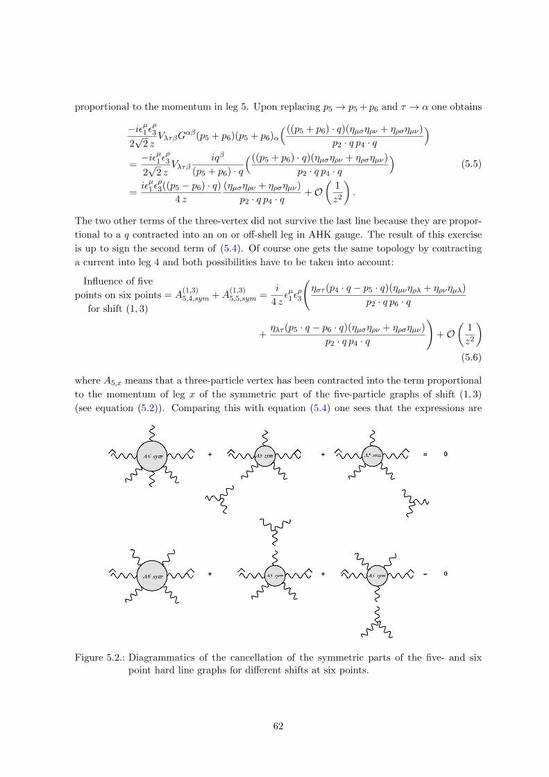
proportional to the momentum in leg 5. Upon replacing p5 → p5 + p6 and τ → α one obtains
−iεµ1 ερ32√
2 zVλτβG
αβ(p5 + p6)(p5 + p6)α
(((p5 + p6) · q)(ηµσηρν + ηρσηµν)
p2 · q p4 · q)
=−iεµ1 ερ32√
2 zVλτβ
iqβ
(p5 + p6) · q(((p5 + p6) · q)(ηµσηρν + ηρσηµν)
p2 · q p4 · q)
=iεµ1 ε
ρ3((p5 − p6) · q)
4 z
(ηµσηρν + ηρσηµν)
p2 · q p4 · q+O
(1
z2
).
(5.5)
The two other terms of the three-vertex did not survive the last line because they are propor-
tional to a q contracted into an on or off-shell leg in AHK gauge. The result of this exercise
is up to sign the second term of (5.4). Of course one gets the same topology by contracting
a current into leg 4 and both possibilities have to be taken into account:
Influence of five
points on six points
for shift (1, 3)
= A(1,3)5,4,sym +A
(1,3)5,5,sym =
i
4 zεµ1 ε
ρ3
(ηστ (p4 · q − p5 · q)(ηµνηρλ + ηρνηµλ)
p2 · q p6 · q
+ηλτ (p5 · q − p6 · q)(ηµσηρν + ηρσηµν)
p2 · q p4 · q
)+O
(1
z2
)
(5.6)
where A5,x means that a three-particle vertex has been contracted into the term proportional
to the momentum of leg x of the symmetric part of the five-particle graphs of shift (1, 3)
(see equation (5.2)). Comparing this with equation (5.4) one sees that the expressions are
Figure 5.2.: Diagrammatics of the cancellation of the symmetric parts of the five- and sixpoint hard line graphs for different shifts at six points.
62

identical up to sign and their sum vanishes. Connecting a current to the second leg of the
five-point symmetric part will result in canceling terms of the symmetric part of the (1, 4)
six leg graphs. The other shifts work along the same lines. This is represented in figure 5.2.
Connecting a current to the second leg of the five-point symmetric part will result in canceling
terms of the symmetric part of the (1, 4) six leg graphs. The other shifts work along the same
lines. This is represented in figure 5.2.
To repeat this once more: each term of the symmetric five-point gluon graphs has to be
treated separately since each of these terms will give rise to contributions for different color
orders/shifts of six-point graphs. Remember that contractions into leg 4 and 5 gave rise to
terms at the color ordering (123456) whereas a contraction into leg 2 yielded contributions at
(123456) each canceling symmetric terms at six points. This is generic since all legs are kept
off-shell, so it follows that the symmetric parts will cancel each other at higher points, too.
Therefore the large-z behavior of purely gluonic integrands subjected to non-adjacent shifts
is given by equation (4.44).
5.1.2. Minimally coupled scalar contributions
In this subsection it will be shown that the scaling behavior of the integrand under a non-
adjacent BCFW shift of two gluons does not change if minimal scalar-gluon couplings are
included. This involves analyzing all scalar contributions to hard-line graphs up to order
∼ (z−1). The scalar Feynman rules are given in appendix B. Note that these rules are for
adjoint matter, for fundamental matter one simply restricts to the diagrams where the scalar
legs are adjacent.
At four points the new graphs to be considered consist of two gluons and two scalars. They
are drawn in figure C.3. Let 1, 3 denote the gluons and 2, 4 denote the scalars. The sum of
the three graphs evaluates to
A4pt ∼ εµ1 ερ3
(iηµρ +
i
z p4 · q(− Pρp2µ + Pµp2ρ
))+O
(1
z2
)(5.7)
where P = p1 + p3. This shows the scaling behavior of equation (4.44).
The analysis of the large-z behavior of five legged scalar/gluon graphs is similar for all
possibilities of particle combinations. Take for example particles 1 to 3 to be gluons and
particle 4 and 5 to be scalars. The Feynman graphs for this choice are depicted in figure C.4.
The result of the sum under the non-adjacent shift is given by
A5pt ∼ εµ1 ερ3
(i(ηµν (p5 − p4)ρ − ηνρ (p5 − p4)µ
)
2√
2 z p2 · q
)+O
(1
z2
). (5.8)
This result is antisymmetric in the indices of the shifted legs at order ∼ (z−1). Note that in
contrast to the five-point gluon diagrams no symmetric piece remains. The other possibilities
of choosing particles yield the same result.
At six points the number of graphs increases significantly. One can pick either two gluons
63

and four scalars or vice versa. The first case is unimportant because the graphs one would
have to consider scale as ∼(z−2). Hence the only diagrams to be taken into account here have
four gauge bosons and two scalars. They are depicted in figure C.5 for a particular distribution
of particles with the shift (1, 4). Summing all the graphs one finds a non-vanishing symmetric
part at order ∼(z−1) given by
A6ptsym ∼ εµ1 ερ4
(i(p5 · q − p6 · q) (ηµνηρσ + ηρµησν)
4z p2 · q p3 · q
)+O
(1
z2
). (5.9)
This parallels the case of six gluons, where the five-point gluonic graphs have to be taken
into account. Since the five-scalar-gluon graphs are already antisymmetric at order ∼ (z−1)
the missing contributions can only come from the five-gluon graphs. The five-point gluon
diagrams leading to the sought-for cancellation are shift (1, 4) diagrams with a scalar-scalar-
gluon vertex contracted into leg five. The result of these graphs is given by (5.9) with opposite
sign and consequently the symmetric part vanishes when summed.
Up to now the scalar legs have been adjacent. For non-adjacent scalar legs the sum of
all diagrams has been checked explicitly to be antisymmetric at order ∼ (z−1) by itself at
both five and six points. Note that the symmetric terms of the all-gluon five-point graphs
uncovered above do not influence any six point graph that has two non-adjacent scalar legs.
Therefore the large-z behavior of integrands of minimally coupled scalar theories subjected
a to non-adjacent shift of two gluons is given by equation (4.44).
Figure 5.3.: Diagrammatics of the cancellation of the symmetric parts of the five and six pointhard line graphs for different shifts at six points for scalar/gluon graphs.
64
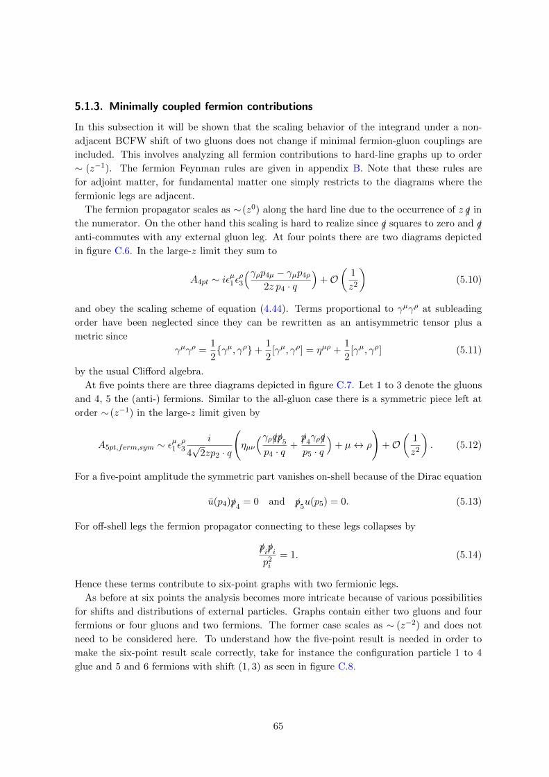
5.1.3. Minimally coupled fermion contributions
In this subsection it will be shown that the scaling behavior of the integrand under a non-
adjacent BCFW shift of two gluons does not change if minimal fermion-gluon couplings are
included. This involves analyzing all fermion contributions to hard-line graphs up to order
∼ (z−1). The fermion Feynman rules are given in appendix B. Note that these rules are
for adjoint matter, for fundamental matter one simply restricts to the diagrams where the
fermionic legs are adjacent.
The fermion propagator scales as ∼(z0) along the hard line due to the occurrence of z /q in
the numerator. On the other hand this scaling is hard to realize since /q squares to zero and /q
anti-commutes with any external gluon leg. At four points there are two diagrams depicted
in figure C.6. In the large-z limit they sum to
A4pt ∼ iεµ1 ερ3(γρp4µ − γµp4ρ
2z p4 · q)
+O(
1
z2
)(5.10)
and obey the scaling scheme of equation (4.44). Terms proportional to γµγρ at subleading
order have been neglected since they can be rewritten as an antisymmetric tensor plus a
metric since
γµγρ =1
2{γµ, γρ}+
1
2[γµ, γρ] = ηµρ +
1
2[γµ, γρ] (5.11)
by the usual Clifford algebra.
At five points there are three diagrams depicted in figure C.7. Let 1 to 3 denote the gluons
and 4, 5 the (anti-) fermions. Similar to the all-gluon case there is a symmetric piece left at
order ∼(z−1) in the large-z limit given by
A5pt,ferm,sym ∼ εµ1 ερ3i
4√
2zp2 · q
(ηµν
(γρ/q/p5
p4 · q+/p4γρ/q
p5 · q)
+ µ↔ ρ
)+O
(1
z2
). (5.12)
For a five-point amplitude the symmetric part vanishes on-shell because of the Dirac equation
u(p4)/p4= 0 and /p5
u(p5) = 0. (5.13)
For off-shell legs the fermion propagator connecting to these legs collapses by
/pi/pip2i
= 1. (5.14)
Hence these terms contribute to six-point graphs with two fermionic legs.
As before at six points the analysis becomes more intricate because of various possibilities
for shifts and distributions of external particles. Graphs contain either two gluons and four
fermions or four gluons and two fermions. The former case scales as ∼ (z−2) and does not
need to be considered here. To understand how the five-point result is needed in order to
make the six-point result scale correctly, take for instance the configuration particle 1 to 4
glue and 5 and 6 fermions with shift (1, 3) as seen in figure C.8.
65
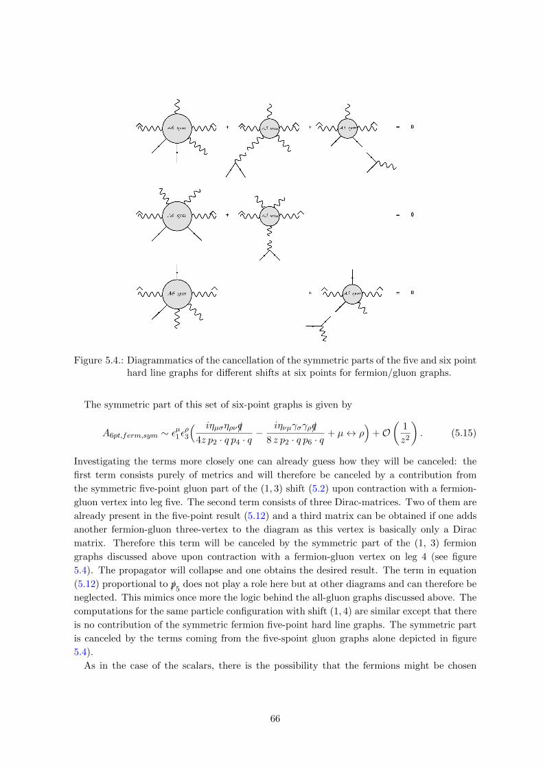
Figure 5.4.: Diagrammatics of the cancellation of the symmetric parts of the five and six pointhard line graphs for different shifts at six points for fermion/gluon graphs.
The symmetric part of this set of six-point graphs is given by
A6pt,ferm,sym ∼ εµ1 ερ3( iηµσηρν/q
4z p2 · q p4 · q− iηνµγσγρ/q
8 z p2 · q p6 · q+ µ↔ ρ
)+O
(1
z2
). (5.15)
Investigating the terms more closely one can already guess how they will be canceled: the
first term consists purely of metrics and will therefore be canceled by a contribution from
the symmetric five-point gluon part of the (1, 3) shift (5.2) upon contraction with a fermion-
gluon vertex into leg five. The second term consists of three Dirac-matrices. Two of them are
already present in the five-point result (5.12) and a third matrix can be obtained if one adds
another fermion-gluon three-vertex to the diagram as this vertex is basically only a Dirac
matrix. Therefore this term will be canceled by the symmetric part of the (1, 3) fermion
graphs discussed above upon contraction with a fermion-gluon vertex on leg 4 (see figure
5.4). The propagator will collapse and one obtains the desired result. The term in equation
(5.12) proportional to /p5does not play a role here but at other diagrams and can therefore be
neglected. This mimics once more the logic behind the all-gluon graphs discussed above. The
computations for the same particle configuration with shift (1, 4) are similar except that there
is no contribution of the symmetric fermion five-point hard line graphs. The symmetric part
is canceled by the terms coming from the five-spoint gluon graphs alone depicted in figure
5.4).
As in the case of the scalars, there is the possibility that the fermions might be chosen
66
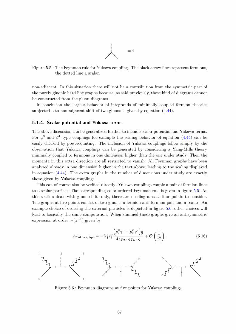
= i
Figure 5.5.: The Feynman rule for Yukawa coupling. The black arrow lines represent fermions,the dotted line a scalar.
non-adjacent. In this situation there will not be a contribution from the symmetric part of
the purely gluonic hard line graphs because, as said previously, these kind of diagrams cannot
be constructed from the gluon diagrams.
In conclusion the large-z behavior of integrands of minimally coupled fermion theories
subjected a to non-adjacent shift of two gluons is given by equation (4.44).
5.1.4. Scalar potential and Yukawa terms
The above discussion can be generalized further to include scalar potential and Yukawa terms.
For φ3 and φ4 type couplings for example the scaling behavior of equation (4.44) can be
easily checked by powercounting. The inclusion of Yukawa couplings follow simply by the
observation that Yukawa couplings can be generated by considering a Yang-Mills theory
minimally coupled to fermions in one dimension higher than the one under study. Then the
momenta in this extra direction are all restricted to vanish. All Feynman graphs have been
analyzed already in one dimension higher in the text above, leading to the scaling displayed
in equation (4.44). The extra graphs in the number of dimensions under study are exactly
those given by Yukawa couplings.
This can of course also be verified directly. Yukawa couplings couple a pair of fermion lines
to a scalar particle. The corresponding color-ordered Feynman rule is given in figure 5.5. As
this section deals with gluon shifts only, there are no diagrams at four points to consider.
The graphs at five points consist of two gluons, a fermion anti-fermion pair and a scalar. An
example choice of ordering the external particles is depicted in figure 5.6, other choices will
lead to basically the same computation. When summed these graphs give an antisymmetric
expression at order ∼(z−1) given by
AYukawa, 5pt = −iεµ1 ερ3
(pµ2γ
ρ − pρ2γµ)/q
4z p2 · q p5 · q+O
(1
z2
). (5.16)
1 2 3
45
Figure 5.6.: Feynman diagrams at five points for Yukawa couplings.
67

This leaves the six point graphs. For instance the graphs which arise by adding a gluon
directly on the scalar vertex of the center diagram in figure 5.6. The complete list of diagrams
belonging to this class is depicted in figure C.10. Under a shift of two non-adjacent gluons,
say (1,4) ((1,3) works along the same lines) the sum of these is antisymmetric at subleading
order
AYukawa,6pt = iεµ1 εσ4
(ηµργσ − ηρσγµ
)/q
4√
2zp6 · q(p5 · q + p6 · q)+O
(1
z2
). (5.17)
Other possible inclusions of an additional gluon will give rise to diagrams that start at ∼(z−2).
Comments
It has been proven in this section that BCFW shifts of two non-color adjacent gluons on
integrands of Yang-Mills theories minimally coupled to scalar or spin 1/2 matter with pos-
sible scalar or Yukawa terms scale as given in equation (4.44). The calculation, although
conceptually straightforward, is more intricate compared to the color adjacent case reviewed
in chapter 2 and a lot more complicated than obtaining the improved scaling behavior for
tree-level amplitudes from color-kinematics duality. In general, using the same powercounting
strategy one can derive the improved scaling behavior of color-ordered Yang-Mills tree ampli-
tudes under permutations (4.47) and cyclic sums (4.49) for any number of permuted legs in
this way. This was worked out by us up to O(1/z2) in the background field gauge in reference
[58]. Note that the above results on shifts of two gluons can be used in a supersymmetric
field theory to obtain shifts of certain fermions and scalar pairs. This has been explained and
derived in detail in the same reference.
As was briefly mentioned in section 4.1.4 the improved scaling of Yang-Mills tree amplitudes
can also be used to obtain certain decoupling relations for one-loop bubble and triangle
coefficients (4.51) and rational terms (4.52). Moreover, as was remarked in chapter 4 the
improved Yang-Mills integrand scaling for a non-adjacent shift to all loop orders gives rise
to the extension of the BCJ relations at the one-loop level for the Yang-Mills integrand. For
more on these two points, again consult our paper [58]. Recall that the integrand BCJ relation
was used to argue that a a solution to the linear map approach to color-kinematics duality
on the integrand level at one loop can be found (compare (4.61)).
5.2. Numerator scaling off-shell
In this section it will be argued that the large-z behavior of the kinematic numerators at
tree and integrand level can actually be seen from Feynman diagrams directly using standard
power counting. The main point will be to use color Jacobi relations to relate different
contributions so that cancellations are achieved in the sum over Feynman graphs and the
large-z scaling of the kinematic numerators found in the previous chapter will be – at least
conceptually – reproduced.
68

5.2.1. Comparison to BCFW shifts directly via Feynman graphs
To obtain the large-z shift of kinematic numerators from Feynman diagrams directly Feynman
rules in the Feynman-’t Hooft gauge will be used and the gluon propagator will be put in
the lightcone AHK gauge as before in this chapter. For brevity only the leading large-z
contribution will be considered in the following but the subleading ones can be treated along
the same lines. Remember that in our conventions the z-dependence flows along the shortest
path between the two shifted legs.
Example: four point Feynman graphs
As was seen already several times, there are only three cubic diagrams to consider at four
points tree level: s, t, and u-channel with the four-vertex absorbed into the cubic graphs
according to the color factors. The cubic representation is then given by
A4 =csnss
+ctntt
+cunuu
. (5.18)
In the following two particle momenta will be BCFW shifted and the other two legs will
remain off-shell. In this way the analysis extends to the integrand. More precisely, it extends
to the Feynman graphs of the integrand with maximally one hard propagator in between the
shifted legs. For graphs with more hard propagators the power counting will become more
complicated as the number of graphs increases but in spirit it is similar. Hence, on the level
of the integrand the leading large-z behavior for this class of diagrams is in a cubic form given
by
I4 =csnss
+ctntt
+cunuu
with cu = cs − ct ⇒ nu = ns − nt (5.19)
Writing down the Feynman graphs and shifting particles 1 and 2 one can extract the large-z
behavior of the kinematic numerators straightforwardly and it follows for the leading power
in z for the three numerators (with indices σ and ρ meaning to be contracted into appropriate
s t u
Figure 5.7.: s, t, and u channel cubic graphs used in the four point example. Hats denote theBCFW-shifted legs.
69
currents)
limz→∞
ns = ε(1)µε(2)ν
(4izηµνηρσp4 · q +O(z0)
)
limz→∞
nt = ε(1)µε(2)ν
(2iz(ηµσηνρ − ηµρηνσ + ηµνηρσ)p4 · q +O(z0)
)
limz→∞
nu = ε(1)µε(2)ν
(2iz(−ηµσηνρ + ηµρηνσ + ηµνηρσ)p4 · q +O(z0)
).
(5.20)
While these numerators satisfy the Jacobi relation above at leading order in z (this is special
for four points) they do not yet have the form one would expect from the discussion in the
previous sections, i.e z times a metric between the shifted legs. To get to this form one has to
make use of the color Jacobi relations. It can be used to shift all terms not proportional to the
metric from nu to nt and ns in (5.19). In the former numerator these will cancel with the other
terms not proportional to ηµν and in the latter numerator these terms will become subleading
in the large-z limit. This corresponds to shifting terms from the four-vertex between different
kinematic channels. After some algebraic gymnastics one arrives at
limz→∞
ns = ε(1)µε(2)ν
(4izηµνηρσp4 · q +O(z0)
)
limz→∞
nt = ε(1)µε(2)ν
(2izηµνηρσp4 · q +O(z0)
)
limz→∞
nu = ε(1)µε(2)ν
(2izηµνηρσp4 · q +O(z0)
)(5.21)
which nicely mirrors the leading part of the result (4.42) obtained using generalized inverses
for four points. It can be shown in a similar way that the subleading pieces are antisymmetric.
Higher points and inclusion of matter
In principle this procedure can be done in a similar fashion at higher points including the
subleading parts. As the number of Jacobi relations increases quite rapidly with the number
of points this becomes, however, more and more intricate. We could reproduce the scaling
(4.42) in this direct Feynman graph approach up to including six points and our suspicion is
that this can be done at any number of points. Furthermore, similar steps can be repeated
for scalars and fermions in the adjoint and one arrives at the same result as before. This was
also checked up to including six points.
5.2.2. BCFW shifts versus color-kinematic duality
The problem with the direct approach using Feynman diagrams is – as already mentioned
many times – that the numerators obtained in this way do not satisfy the Jacobi relations
beyond four points directly. Instead they obey
{ni − nj + nk = ua, a = 1, ...,#Jacobis} (5.22)
where the right-hand side is non-vanishing and different for each Jacobi relation. One can now
make use of gauge transformations on the numerators to bring them into a BCJ satisfying
70

form. For example by implementing a numerator shift at tree level given by
ni → ni + ∆i with∑
i
ci∆i
si= 0 ∀i. (5.23)
At tree level this works at follows: Following [11] there are (2n − 5)!! kinematic numerators
/ color factors at n points tree level. These obey (n−3)(2n−5)!3 Jacobi relations which involve
quite a lot of redundancy so that the number of non-redundant Jacobi relations is given
by (2n − 5)!! − (n − 2)!. In other words (n − 2)! kinematic numerators / color factors are
independent. Having constructed the numerators using Feynman diagrams one would have
consequently obtained (2n−5)!!−(n−2)! non-redundant Jacobi relations that are not satisfied
{ni − nj + nk = ua, a = 1, ..., (2n− 5)!!− (n− 2)!}. (5.24)
By enforcing a generalized gauge transformation on all (2n − 5)!! kinematic numerators the
right hand side of the non-redundant Jacobi relations can be brought to zero by requiring (in
addition to the gauge condition above)
{∆i −∆j + ∆k = ua, a = 1, ..., (2n− 5)!!− (n− 2)!} (5.25)
so that the non-vanishing right side of the kinematic Jacobi relations gets cancelled. Based
on pure counting the generalized gauge condition would give (n− 2)! conditions on the shifts
so that one the number of total equations for the shifts ∆ is
(2n− 5)!!− (n− 2)!︸ ︷︷ ︸#Jacobi relations to bring to zero
+ (n− 2)!︸ ︷︷ ︸# gauge conditions
= (2n− 5)!! (5.26)
i.e. (2n−5)!! equations for (2n−5)!! shifts (i.e. variables) which means that in principle there
should be a solution to this system of equation. This of course is hard to handle already
at five points as the expressions involved become quite unhandy. Moreover, this raises the
question if applying the generalized gauge transformations that bring the numerators into a
BCJ satisfying form respects the large-z scaling? The answer to this is – especially in view
of the results and discussion in chapter 4 – positive as we know that there are explicit sets of
numerators that have the same large-z scaling as here at any points. In principle up to the
subtleties mentioned several times, the same reasoning applies on the level of the integrand
if color-dual numerators at loop level exist.
71
72

6. Summary and Outlook
In this thesis a novel symmetry of Yang-Mills theory amplitudes called color-kinematics dual-
ity was investigated from different complementing viewpoints. Color-kinematics duality offers
a completely new perspective on gauge and gravity theories and explains many previously not
fully understood properties of gauge and gravity amplitudes as its consequence. The duality
is a key mechanism behind cancellations found in scattering amplitudes of gauge and gravity
theories which are not obvious from Feynman graphs and so the duality plays a decisive role
in investigating whether maximal supergravity is perturbatively UV finite or not.
In the first part of this thesis, we showed how color-kinematics duality can be made manifest
at the one-loop level in (pure) Yang-Mills theory for rational amplitudes, i.e. all-plus and one-
minus amplitudes. The former arise in the self-dual sector of the theory. This is especially
simple since it only has a cubic interaction vertex and hence color-kinematics duality can
be readily shown for the all-plus one-loop amplitudes even on the level of the Lagrangian.
The results for the self-dual sector could then be extended to also incorporate one-minus
amplitudes. Although computations of these amplitudes would in principle include quartic
vertices these could be eliminated by a certain gauge choice so that effectively one only has to
consider (two types) of cubic vertices. In this way also one-minus amplitudes manifestly obey
color-kinematics duality. As a neat example the all-plus and one-minus four-point gravity
amplitudes in N = 0 extended Einstein gravity were computed through the double copy
construction and agreement with known results from the literature found.
Secondly, the implications of color-kinematics duality for powercounting in gravity theories
were studied. A reformulation of the duality in terms of linear maps was particularly suited for
this endeavor; in this way encoding the duality in a matrix F and its generalized inverse F+.
The properties of these matrices could then be extracted by studying them in a appropriate
basis of trivalent scalar theories. As specific examples for how this refines powercounting in
gravity theories, the behavior of gravity integrands under large BCFW shifts in quite generic
gravity theories to all loop orders was derived. Up to certain assumptions and subtleties
inherent to the duality that were addressed, we found massive cancellations for the involved
powercounting behavior that are not at all obvious from a naıve Feynman diagrammatic
point of view. In fact, we could even show that the scaling under the large BCFW shifts is
independent of the loop order and that the reason for this is precisely the duality. In addition,
we showed that the duality also implies drastic cancellations for gauge theories amplitudes
under permutation and cyclic sums that gave rise to certain Yang-Mills relations at one-loop.
Furthermore, we used the same techniques as for the BCFW shifts to study the UV behavior
of N = 8 supergravity. In doing so the related results of Bern et al. could be interpreted and
understood from the linear map perspective using powercounting. Based on our method we
73
found indications for the finiteness of maximal supergravity at five loops in five dimensions
(i.e. seven loops in four dimensions) if certain tadpoles diagrams were to be included in the
actual loop computation. Moreover, our approach suggests that there will be a divergence at
eight loops in four dimensions if no further improvements appear.
Lastly, we have considered color-kinematics duality in terms of Feynman diagrams from
an off-shell point of view. Using Feynman diagrams we have reproduced some of the re-
sults of the previous chapter like the improved large BCFW shift behavior of gauge theories
amplitudes/integrands to all loop orders under non-adjacent BCFW shifts. Moreover, we
have reproduced the scaling of the kinematic numerators at four points diagrammatically for
large BCFW shifts. This could be extended to six points including scalars/fermions in the
adjoint. It was seen that this approach, while technically straightforward, is quite tedious
due to the large number of graphs to consider. Furthermore, it has the distinct disadvantage
that numerators constructed directly using Feynman graphs are not manifestly color-dual.
Nonetheless, the mere fact that we could reproduce some of the results in this way offers
quite nice indications from a complementing viewpoint that the duality holds true in general
at the loop level.
Opportunities for future research based on the above results present themselves. One
obvious and very ambitious question to study is if it is possible to extend the results from the
self-dual sector of Yang-Mills theory to the full theory. In other words: would it be possible
to cast the whole Lagrangian into an explicitly color-kinematics manifest form? Achieving
this would be equivalent to a general proof of color-kinematics duality and would extend it
to other observables like form factors and correlation functions. As it was recently shown
for some examples in [55] that form factors in N = 4 can be brought in a color-dual form it
seems reasonable to suspect that a manifestly color-dual Lagrangian exists. This is closely
connected to work from the late 1990s which aimed at constructing a gravity Lagrangian from
gauge theory [179] and, more recently, to insights based on double field theory and generalized
geometry [180, 181]. These closely related approaches make manifest a factorization of the
(super)gravity Lagrangian into so-called ‘left’ and ‘right’ parts and serve in this way as the
first step towards a Lagrangian-based proof of color-kinematics duality. It remains to show,
however, that the left and right factors actually correspond to usual Yang-Mills theories.
Proving color-kinematics duality in general would also be more than welcome as it would
sharpen the results of the linear map approach to the duality. In addition, a better under-
standing of the precise implementation of color-kinematics duality is necessary in order to
answer the question of which trivalent diagrams to include in the construction. This also has
direct impact for addressing cancellations implied by the duality and most importantly the
question of UV-finiteness of maximal supergravity.
The gravity integrand was shown to behave like 1/z2 for large BCFW shifts. This good
behavior implies the existence of on-shell recursion relations for the gravity integrand. It
would be very interesting to derive these and moreover, it would also be interesting to find
out whether this improved behavior under shifts implies the existence of bonus relations as is
known from tree level [149].
74
Another related interesting question is how much more amplitude relations does color-
kinematics duality imply. It is well-known that the tree-level BCJ relations are due to the
duality. Moreover, it was shown in [101] that certain relations for rational one-loop amplitudes
are caused by color-kinematics duality, too. It would be interesting to investigate how much
further this can be pushed as there are more amplitude relations known (see e.g. [123]) whose
origins have not been explained yet. It is also closely connected to the question how many
independent amplitudes there are at loop level. This seems to be closely related to Eulerian
numbers1 [182, 183] but it has never been made precise.
All of this shows that color-kinematics duality most certainly deserves further study. It
has already provided enormous insights into the structure of scattering amplitudes in gauge
and gravity theories and based on these results it is very reasonable to suspect that a deeper
understanding of color-kinematics duality will uncover even more completely new and un-
expected perspectives on scattering amplitudes – perhaps even on the very formulation of
quantum field theory itself.
1The author is grateful to Henrik Johansson for pointing this out.
75
76
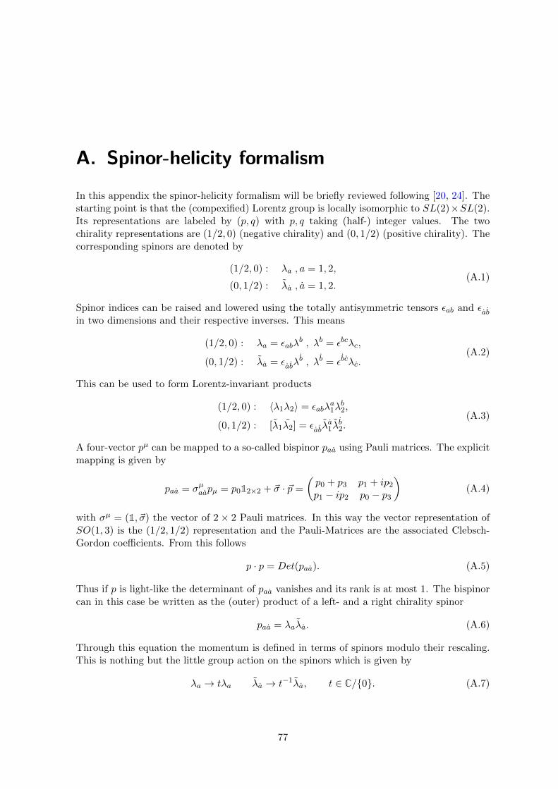
A. Spinor-helicity formalism
In this appendix the spinor-helicity formalism will be briefly reviewed following [20, 24]. Thestarting point is that the (compexified) Lorentz group is locally isomorphic to SL(2)×SL(2).Its representations are labeled by (p, q) with p, q taking (half-) integer values. The twochirality representations are (1/2, 0) (negative chirality) and (0, 1/2) (positive chirality). Thecorresponding spinors are denoted by
(1/2, 0) : λa , a = 1, 2,
(0, 1/2) : λa , a = 1, 2.(A.1)
Spinor indices can be raised and lowered using the totally antisymmetric tensors εab and εabin two dimensions and their respective inverses. This means
(1/2, 0) : λa = εabλb , λb = εbcλc,
(0, 1/2) : λa = εabλb , λb = εbcλc.
(A.2)
This can be used to form Lorentz-invariant products
(1/2, 0) : 〈λ1λ2〉 = εabλa1λ
b2,
(0, 1/2) : [λ1λ2] = εabλa1λ
b2.
(A.3)
A four-vector pµ can be mapped to a so-called bispinor paa using Pauli matrices. The explicitmapping is given by
paa = σµaapµ = p012×2 + ~σ · ~p =
(p0 + p3 p1 + ip2
p1 − ip2 p0 − p3
)(A.4)
with σµ = (1, ~σ) the vector of 2× 2 Pauli matrices. In this way the vector representation ofSO(1, 3) is the (1/2, 1/2) representation and the Pauli-Matrices are the associated Clebsch-Gordon coefficients. From this follows
p · p = Det(paa). (A.5)
Thus if p is light-like the determinant of paa vanishes and its rank is at most 1. The bispinorcan in this case be written as the (outer) product of a left- and a right chirality spinor
paa = λaλa. (A.6)
Through this equation the momentum is defined in terms of spinors modulo their rescaling.This is nothing but the little group action on the spinors which is given by
λa → tλa λa → t−1λa, t ∈ C/{0}. (A.7)
77

For real momenta the two spinors λ and λ are just complex conjugates of each other. Forcomplexified momenta they are independent. We always adopt the latter viewpoint.
Equation (A.5) can be generalized for two different four-vectors. In this way scalar productsfor light-like four-vectors can be reexpressed as products of spinors brackets by
p · q =1
2〈λpλq〉[λqλp]. (A.8)
In addition to the spinor brackets introduced above there are also longer strings of spinorbrackets possible. For instance, if one sandwiches some general four-vector P between twoopposite helicity spinor brackets using gamma matrices one finds (writing i and j instead ofλi and λj)
〈i|/P |j] = λiaPbbλjaεabεab = [j|/P |i〉. (A.9)
One often suppresses writing the slash explicitly. Note that because of chirality the followingspinor contractions vanish
〈ij] = 0,
[ij〉 = 0.(A.10)
If P is light-like, equation (A.9) is by (A.6) equivalent to
〈i|/P |j] = 〈iP 〉[Pj]. (A.11)
This can be generalized to arbitrarily long spinor bracket strings. For instance, one couldwrite down
〈i|/P /Q|j〉 = 〈iP 〉[PQ]〈Qj〉,〈i|/P /Q /K|j] = 〈iP 〉[PQ]〈QK〉[Kj]. (A.12)
for P ,K,Q light-like vectors.Spinor brackets satisfy the Schouten identity which is nothing but a consequence of the
spinors living in a 2-dimensional space. The identity is given by
〈ij〉〈kl〉+ 〈ik〉〈lj〉+ 〈il〉〈jk〉 = 0 (A.13)
and similarly for the other type of spinor bracket.In the same way that light-like momenta can be written in terms of spinors also polarization
vectors can be mapped to spinors. For instance one can write gluon helicities in this way as
ε−aa = −√
2λaµa[λµ]
ε+aa = −√
2µaλa〈µλ〉 (A.14)
with µ and µ reference spinors.
78

B. Color-ordered Feynman rules
This appendix contains the color-ordered Feynman rules of Yang-Mills theory minimally cou-pled to scalar or spin one-half matter in AHK gauge.
α
β
γ
p
k
q
= −i√2(ηαβ(p− k)γ + ηβγ(k − q)α + ηγα(q − p)β)
= i√2(p− q)α
α = −iγα√2
q
p
α
β
= −i2 ηαβ
p
= −ip2(ηαβ − pαqβ+pβqα
p·q )
p
= iγ·pp2
p
= −ip2
α β
γδ
= iηαγηβδ − i2(ηαβηγδ + ηαδηβγ)
α
β
= iηαβ
Figure B.1.: Color-ordered Feynman rules for gluons (wiggly lines), scalars (dotted lines), andfermions (straight lines).
79
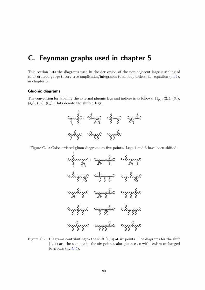
C. Feynman graphs used in chapter 5
This section lists the diagrams used in the derivation of the non-adjacent large-z scaling ofcolor-ordered gauge theory tree amplitudes/integrands to all loop orders, i.e. equation (4.44),in chapter 5.
Gluonic diagrams
The convention for labeling the external gluonic legs and indices is as follows: (1µ), (2ν), (3ρ),(4σ), (5τ ), (6λ). Hats denote the shifted legs.
1
2
3
45
Figure C.1.: Color-ordered gluon diagrams at five points. Legs 1 and 3 have been shifted.
1
2
3
456
Figure C.2.: Diagrams contributing to the shift (1, 3) at six points. The diagrams for the shift(1, 4) are the same as in the six-point scalar-gluon case with scalars exchangedto gluons (fig C.5).
80
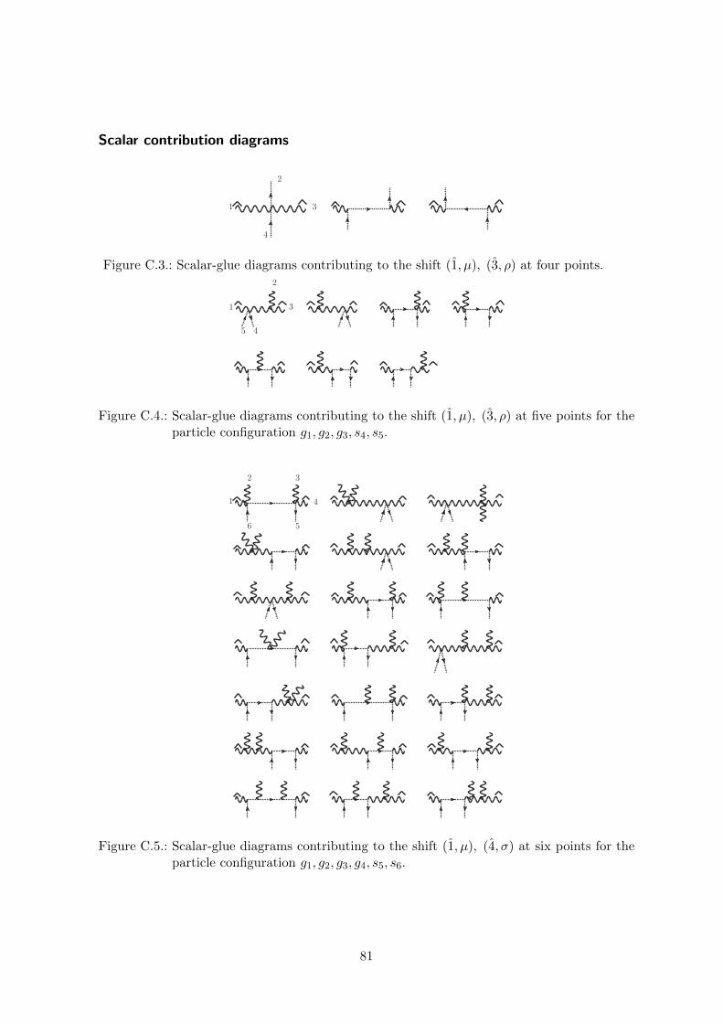
Scalar contribution diagrams
1
2
3
4
Figure C.3.: Scalar-glue diagrams contributing to the shift (1, µ), (3, ρ) at four points.
1
2
3
45
Figure C.4.: Scalar-glue diagrams contributing to the shift (1, µ), (3, ρ) at five points for theparticle configuration g1, g2, g3, s4, s5.
1
2 3
4
56
Figure C.5.: Scalar-glue diagrams contributing to the shift (1, µ), (4, σ) at six points for theparticle configuration g1, g2, g3, g4, s5, s6.
81
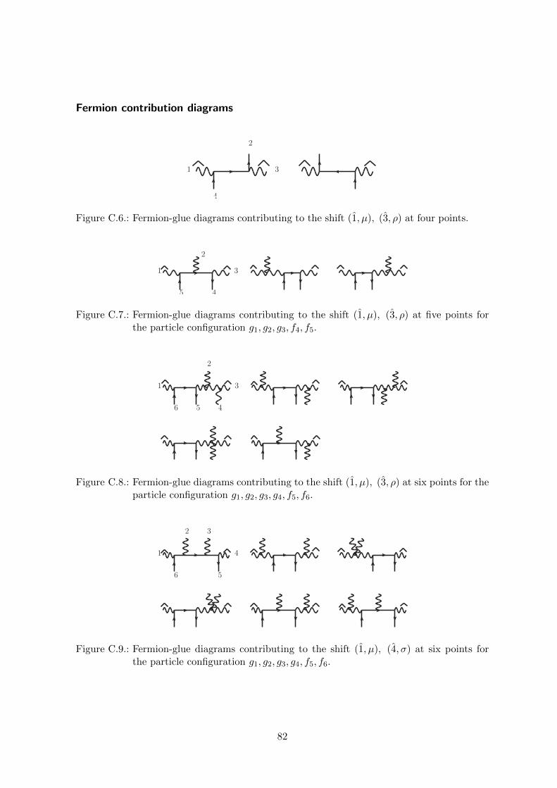
Fermion contribution diagrams
1
2
3
4
Figure C.6.: Fermion-glue diagrams contributing to the shift (1, µ), (3, ρ) at four points.
1
2
3
45
Figure C.7.: Fermion-glue diagrams contributing to the shift (1, µ), (3, ρ) at five points forthe particle configuration g1, g2, g3, f4, f5.
1
2
3
456
Figure C.8.: Fermion-glue diagrams contributing to the shift (1, µ), (3, ρ) at six points for theparticle configuration g1, g2, g3, g4, f5, f6.
1
2 3
4
56
Figure C.9.: Fermion-glue diagrams contributing to the shift (1, µ), (4, σ) at six points forthe particle configuration g1, g2, g3, g4, f5, f6.
82
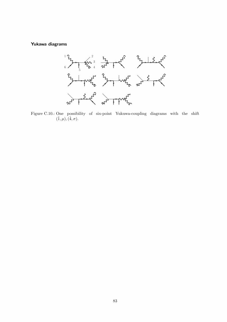
Yukawa diagrams
1 2
3
45
6
Figure C.10.: One possibility of six-point Yukuwa-coupling diagrams with the shift(1, µ), (4, σ).
83

84
Bibliography
[1] S. Glashow, Partial Symmetries of Weak Interactions, Nucl.Phys. 22 (1961) 579–588.
[2] S. Weinberg, A Model of Leptons, Phys.Rev.Lett. 19 (1967) 1264–1266.
[3] M. Gell-Mann, Quarks, Acta Phys.Austriaca Suppl. 9 (1972) 733–761.
[4] D. Gross and F. Wilczek, Ultraviolet Behavior of Nonabelian Gauge Theories,Phys.Rev.Lett. 30 (1973) 1343–1346.
[5] D. Gross and F. Wilczek, Asymptotically Free Gauge Theories. 1, Phys.Rev. D8(1973) 3633–3652.
[6] S. Weinberg, Nonabelian Gauge Theories of the Strong Interactions, Phys.Rev.Lett. 31(1973) 494–497.
[7] Particle Data Group Collaboration, J. Beringer et. al., Review of Particle Physics(RPP), Phys.Rev. D86 (2012) 010001.
[8] S. J. Parke and T. R. Taylor, An amplitude for n gluon scattering, Phys. Rev. Lett. 56(1986) 2459.
[9] G. ’t Hooft and M. Veltman, One loop divergencies in the theory of gravitation,Annales Poincare Phys.Theor. A20 (1974) 69–94.
[10] H. Kawai, D. Lewellen, and S. Tye, A Relation Between Tree Amplitudes of Closedand Open Strings, Nucl.Phys. B269 (1986) 1.
[11] Z. Bern, J. J. M. Carrasco, and H. Johansson, New Relations for Gauge-TheoryAmplitudes, Phys. Rev. D78 (2008) 085011, [arXiv:0805.3993].
[12] J. A. Wheeler, On the mathematical description of light nuclei by the method ofresonating group structure, Phys. Rev. 52 (Dec, 1937) 1107–1122.
[13] W. Heisenberg, The observable quantities in the theory of elementary particles,Z.Phys. 120 (1943) 513.
[14] N. Arkani-Hamed, F. Cachazo, and J. Kaplan, What is the Simplest Quantum FieldTheory?, JHEP 1009 (2010) 016, [arXiv:0808.1446].
[15] N. Arkani-Hamed, “Interview with Science Watch.”http://archive.sciencewatch.com/ana/st/super/12junSTSuperHamed.
[16] S. Mandelstam, Light Cone Superspace and the Ultraviolet Finiteness of the N=4Model, Nucl.Phys. B213 (1983) 149–168.
85
[17] R. Roiban, M. Spradlin, and A. Volovich, Scattering amplitudes in gauge theories:progress and outlook, Journal of Physics A: Mathematical and Theoretical 44 (2011),no. 45 450301.
[18] N. Beisert, C. Ahn, L. F. Alday, Z. Bajnok, J. M. Drummond, et. al., Review ofAdS/CFT Integrability: An Overview, Lett.Math.Phys. 99 (2012) 3–32,[arXiv:1012.3982].
[19] L. J. Dixon, Calculating scattering amplitudes efficiently, hep-ph/9601359.
[20] R. Britto, “Lecture Notes: Introduction to Scattering Amplitudes.”http://ipht.cea.fr/Docspht/articles/t11/138/public/Cours2011.pdf.
[21] B. Feng and M. Luo, An Introduction to On-shell Recursion Relations,arXiv:1111.5759.
[22] J. Drummond, Hidden Simplicity of Gauge Theory Amplitudes, Class.Quant.Grav. 27(2010) 214001, [arXiv:1010.2418].
[23] F. Cachazo and P. Svrcek, Lectures on twistor strings and perturbative Yang-Millstheory, PoS RTN2005 (2005) 004, [hep-th/0504194].
[24] E. Witten, Perturbative gauge theory as a string theory in twistor space,Commun.Math.Phys. 252 (2004) 189–258, [hep-th/0312171].
[25] F. Cachazo, P. Svrcek, and E. Witten, MHV vertices and tree amplitudes in gaugetheory, JHEP 0409 (2004) 006, [hep-th/0403047].
[26] K. Risager, A Direct proof of the CSW rules, JHEP 0512 (2005) 003,[hep-th/0508206].
[27] G. Georgiou and V. V. Khoze, Tree amplitudes in gauge theory as scalar MHVdiagrams, JHEP 0405 (2004) 070, [hep-th/0404072].
[28] G. Georgiou, E. N. Glover, and V. V. Khoze, Non-MHV tree amplitudes in gaugetheory, JHEP 0407 (2004) 048, [hep-th/0407027].
[29] R. Boels and C. Schwinn, CSW rules for a massive scalar, Phys.Lett. B662 (2008)80–86, [arXiv:0712.3409].
[30] R. Boels and C. Schwinn, Deriving CSW rules for massive scalar legs and pureYang-Mills loops, JHEP 0807 (2008) 007, [arXiv:0805.1197].
[31] A. Brandhuber, B. J. Spence, and G. Travaglini, One-loop gauge theory amplitudes inN=4 super Yang-Mills from MHV vertices, Nucl.Phys. B706 (2005) 150–180,[hep-th/0407214].
[32] J. Bedford, A. Brandhuber, B. J. Spence, and G. Travaglini, A Twistor approach toone-loop amplitudes in N=1 supersymmetric Yang-Mills theory, Nucl.Phys. B706(2005) 100–126, [hep-th/0410280].
86
[33] J. Bedford, A. Brandhuber, B. J. Spence, and G. Travaglini, Non-supersymmetric loopamplitudes and MHV vertices, Nucl.Phys. B712 (2005) 59–85, [hep-th/0412108].
[34] R. Britto, F. Cachazo, and B. Feng, New recursion relations for tree amplitudes ofgluons, Nucl. Phys. B715 (2005) 499–522, [hep-th/0412308].
[35] R. Britto, F. Cachazo, B. Feng, and E. Witten, Direct proof of tree-level recursionrelation in Yang-Mills theory, Phys. Rev. Lett. 94 (2005) 181602, [hep-th/0501052].
[36] R. Roiban, M. Spradlin, and A. Volovich, Dissolving N=4 loop amplitudes into QCDtree amplitudes, Phys.Rev.Lett. 94 (2005) 102002, [hep-th/0412265].
[37] J. Drummond and J. Henn, All tree-level amplitudes in N=4 SYM, JHEP 0904 (2009)018, [arXiv:0808.2475].
[38] N. Arkani-Hamed, J. L. Bourjaily, F. Cachazo, S. Caron-Huot, and J. Trnka, TheAll-Loop Integrand For Scattering Amplitudes in Planar N=4 SYM, JHEP 1101(2011) 041, [arXiv:1008.2958].
[39] N. Arkani-Hamed, J. L. Bourjaily, F. Cachazo, A. B. Goncharov, A. Postnikov, et. al.,Scattering Amplitudes and the Positive Grassmannian, arXiv:1212.5605.
[40] Z. Bern, L. J. Dixon, D. C. Dunbar, and D. A. Kosower, One-Loop n-Point GaugeTheory Amplitudes, Unitarity and Collinear Limits, Nucl. Phys. B425 (1994)217–260, [hep-ph/9403226].
[41] Z. Bern, L. J. Dixon, D. C. Dunbar, and D. A. Kosower, Fusing gauge theory treeamplitudes into loop amplitudes, Nucl.Phys. B435 (1995) 59–101, [hep-ph/9409265].
[42] G. ’t Hooft and M. Veltman, Scalar One Loop Integrals, Nucl.Phys. B153 (1979)365–401.
[43] Z. Bern, L. J. Dixon, and D. A. Kosower, One loop amplitudes for e+ e- to fourpartons, Nucl.Phys. B513 (1998) 3–86, [hep-ph/9708239].
[44] R. Britto, F. Cachazo, and B. Feng, Generalized unitarity and one-loop amplitudes inN=4 super-Yang-Mills, Nucl.Phys. B725 (2005) 275–305, [hep-th/0412103].
[45] D. Forde, Direct extraction of one-loop integral coefficients, Phys.Rev. D75 (2007)125019, [arXiv:0704.1835].
[46] S. Badger, Direct Extraction Of One Loop Rational Terms, JHEP 0901 (2009) 049,[arXiv:0806.4600].
[47] G. Ossola, C. G. Papadopoulos, and R. Pittau, Reducing full one-loop amplitudes toscalar integrals at the integrand level, Nucl.Phys. B763 (2007) 147–169,[hep-ph/0609007].
[48] G. Ossola, C. G. Papadopoulos, and R. Pittau, CutTools: A Program implementingthe OPP reduction method to compute one-loop amplitudes, JHEP 0803 (2008) 042,[arXiv:0711.3596].
87
[49] Z. Bern, L. J. Dixon, and D. Kosower, A Two loop four gluon helicity amplitude inQCD, JHEP 0001 (2000) 027, [hep-ph/0001001].
[50] Z. Bern, A. De Freitas, and L. J. Dixon, Two loop helicity amplitudes for gluon-gluonscattering in QCD and supersymmetric Yang-Mills theory, JHEP 0203 (2002) 018,[hep-ph/0201161].
[51] Z. Bern, J. Carrasco, L. Dixon, H. Johansson, and R. Roiban, Simplifying MultiloopIntegrands and Ultraviolet Divergences of Gauge Theory and Gravity Amplitudes,Phys.Rev. D85 (2012) 105014, [arXiv:1201.5366].
[52] Z. Bern, S. Davies, T. Dennen, and Y.-t. Huang, Absence of Three-Loop Four-PointDivergences in N=4 Supergravity, Phys.Rev.Lett. 108 (2012) 201301,[arXiv:1202.3423].
[53] Z. Bern, S. Davies, T. Dennen, and Y.-t. Huang, Ultraviolet Cancellations inHalf-Maximal Supergravity as a Consequence of the Double-Copy Structure, Phys.Rev.D86 (2012) 105014, [arXiv:1209.2472].
[54] Z. Bern, J. Carrasco, H. Johansson, and R. Roiban, The Five-Loop Four-PointAmplitude of N=4 super-Yang-Mills Theory, Phys.Rev.Lett. 109 (2012) 241602,[arXiv:1207.6666].
[55] R. H. Boels, B. A. Kniehl, O. V. Tarasov, and G. Yang, Color-kinematic Duality forForm Factors, JHEP 1302 (2013) 063, [arXiv:1211.7028].
[56] Z. Bern, T. Dennen, Y.-t. Huang, and M. Kiermaier, Gravity as the Square of GaugeTheory, Phys.Rev. D82 (2010) 065003, [arXiv:1004.0693].
[57] R. H. Boels and R. S. Isermann, New relations for scattering amplitudes in Yang-Millstheory at loop level, Phys.Rev. D85 (2012) 021701, [arXiv:1109.5888].
[58] R. H. Boels and R. S. Isermann, Yang-Mills amplitude relations at loop level fromnon-adjacent BCFW shifts, JHEP 1203 (2012) 051, [arXiv:1110.4462].
[59] R. Monteiro and D. O’Connell, The Kinematic Algebra From the Self-Dual Sector,JHEP 1107 (2011) 007, [arXiv:1105.2565].
[60] T. Bargheer, S. He, and T. McLoughlin, New Relations for Three-DimensionalSupersymmetric Scattering Amplitudes, Phys.Rev.Lett. 108 (2012) 231601,[arXiv:1203.0562].
[61] A. Hodges, Eliminating spurious poles from gauge-theoretic amplitudes,arXiv:0905.1473.
[62] J. Drummond, J. Henn, V. Smirnov, and E. Sokatchev, Magic identities for conformalfour-point integrals, JHEP 0701 (2007) 064, [hep-th/0607160].
[63] J. Drummond, J. Henn, G. Korchemsky, and E. Sokatchev, Dual superconformalsymmetry of scattering amplitudes in N=4 super-Yang-Mills theory, Nucl.Phys. B828(2010) 317–374, [arXiv:0807.1095].
88
[64] A. Brandhuber, P. Heslop, and G. Travaglini, A Note on dual superconformalsymmetry of the N=4 super Yang-Mills S-matrix, Phys.Rev. D78 (2008) 125005,[arXiv:0807.4097].
[65] J. M. Drummond, J. M. Henn, and J. Plefka, Yangian symmetry of scatteringamplitudes in N=4 super Yang-Mills theory, JHEP 0905 (2009) 046,[arXiv:0902.2987].
[66] J. Drummond, J. Henn, G. Korchemsky, and E. Sokatchev, On planar gluonamplitudes/Wilson loops duality, Nucl.Phys. B795 (2008) 52–68, [arXiv:0709.2368].
[67] J. Minahan and K. Zarembo, The Bethe ansatz for N=4 superYang-Mills, JHEP 0303(2003) 013, [hep-th/0212208].
[68] N. Beisert, The complete one loop dilatation operator of N=4 superYang-Mills theory,Nucl.Phys. B676 (2004) 3–42, [hep-th/0307015].
[69] N. Beisert, B. Eden, and M. Staudacher, Transcendentality and Crossing, J.Stat.Mech.0701 (2007) P01021, [hep-th/0610251].
[70] Z. Bern, L. J. Dixon, and V. A. Smirnov, Iteration of planar amplitudes in maximallysupersymmetric Yang-Mills theory at three loops and beyond, Phys.Rev. D72 (2005)085001, [hep-th/0505205].
[71] J. M. Maldacena, The Large N limit of superconformal field theories and supergravity,Adv.Theor.Math.Phys. 2 (1998) 231–252, [hep-th/9711200].
[72] L. F. Alday and J. M. Maldacena, Gluon scattering amplitudes at strong coupling,JHEP 0706 (2007) 064, [arXiv:0705.0303].
[73] L. F. Alday, J. Maldacena, A. Sever, and P. Vieira, Y-system for ScatteringAmplitudes, J.Phys. A43 (2010) 485401, [arXiv:1002.2459].
[74] J. Bartels, V. Schomerus, and M. Sprenger, Multi-Regge Limit of the n-Gluon BubbleAnsatz, JHEP 1211 (2012) 145, [arXiv:1207.4204].
[75] J. Maldacena and A. Zhiboedov, Form factors at strong coupling via a Y-system,JHEP 1011 (2010) 104, [arXiv:1009.1139].
[76] Z. Gao and G. Yang, Y-system for form factors at strong coupling in AdS5 and withmulti-operator insertions, arXiv:1303.2668.
[77] B. Basso, A. Sever, and P. Vieira, Space-time S-matrix and Flux-tube S-matrix atFinite Coupling, arXiv:1303.1396.
[78] J. Drummond, J. Henn, G. Korchemsky, and E. Sokatchev, Conformal Ward identitiesfor Wilson loops and a test of the duality with gluon amplitudes, Nucl.Phys. B826(2010) 337–364, [arXiv:0712.1223].
[79] J. Drummond, J. Henn, G. Korchemsky, and E. Sokatchev, Hexagon Wilson loop =six-gluon MHV amplitude, Nucl.Phys. B815 (2009) 142–173, [arXiv:0803.1466].
89
[80] Z. Bern, L. Dixon, D. Kosower, R. Roiban, M. Spradlin, et. al., The Two-LoopSix-Gluon MHV Amplitude in Maximally Supersymmetric Yang-Mills Theory,Phys.Rev. D78 (2008) 045007, [arXiv:0803.1465].
[81] L. Mason and D. Skinner, The Complete Planar S-matrix of N=4 SYM as a WilsonLoop in Twistor Space, JHEP 1012 (2010) 018, [arXiv:1009.2225].
[82] S. Caron-Huot, Notes on the scattering amplitude / Wilson loop duality, JHEP 1107(2011) 058, [arXiv:1010.1167].
[83] L. F. Alday, B. Eden, G. P. Korchemsky, J. Maldacena, and E. Sokatchev, Fromcorrelation functions to Wilson loops, JHEP 1109 (2011) 123, [arXiv:1007.3243].
[84] B. Eden, G. P. Korchemsky, and E. Sokatchev, From correlation functions toscattering amplitudes, JHEP 1112 (2011) 002, [arXiv:1007.3246].
[85] T. Adamo, M. Bullimore, L. Mason, and D. Skinner, A Proof of the SupersymmetricCorrelation Function / Wilson Loop Correspondence, JHEP 1108 (2011) 076,[arXiv:1103.4119].
[86] A. B. Goncharov, M. Spradlin, C. Vergu, and A. Volovich, Classical Polylogarithms forAmplitudes and Wilson Loops, Phys.Rev.Lett. 105 (2010) 151605, [arXiv:1006.5703].
[87] L. J. Dixon, J. M. Drummond, and J. M. Henn, Bootstrapping the three-loop hexagon,JHEP 1111 (2011) 023, [arXiv:1108.4461].
[88] L. J. Dixon, J. M. Drummond, and J. M. Henn, Analytic result for the two-loopsix-point NMHV amplitude in N=4 super Yang-Mills theory, JHEP 1201 (2012) 024,[arXiv:1111.1704].
[89] V. Del Duca, L. J. Dixon, J. M. Drummond, C. Duhr, J. M. Henn, et. al., Theone-loop six-dimensional hexagon integral with three massive corners, Phys.Rev. D84(2011) 045017, [arXiv:1105.2011].
[90] S. Caron-Huot, Superconformal symmetry and two-loop amplitudes in planar N=4super Yang-Mills, JHEP 1112 (2011) 066, [arXiv:1105.5606].
[91] F. Brown, On the decomposition of motivic multiple zeta values, arXiv:1102.1310.
[92] A. B. Goncharov, Galois symmetries of fundamental groupoids and noncommutativegeometry, ArXiv Mathematics e-prints (2002) [math/0208].
[93] C. Duhr, Hopf algebras, coproducts and symbols: an application to Higgs bosonamplitudes, JHEP 1208 (2012) 043, [arXiv:1203.0454].
[94] O. Schlotterer and S. Stieberger, Motivic Multiple Zeta Values and SuperstringAmplitudes, arXiv:1205.1516.
[95] F. Brown, Single-valued multiple polylogarithms in one variable, C. R. Acad Sci. ParisSer. I (2004), no. 338 527.
90
[96] L. J. Dixon, C. Duhr, and J. Pennington, Single-valued harmonic polylogarithms andthe multi-Regge limit, JHEP 1210 (2012) 074, [arXiv:1207.0186].
[97] J. Pennington, The six-point remainder function to all loop orders in the multi-Reggelimit, JHEP 1301 (2013) 059, [arXiv:1209.5357].
[98] C. R. Mafra, O. Schlotterer, and S. Stieberger, Complete N-Point Superstring DiskAmplitude I. Pure Spinor Computation, arXiv:1106.2645.
[99] C. R. Mafra, O. Schlotterer, and S. Stieberger, Complete N-Point Superstring DiskAmplitude II. Amplitude and Hypergeometric Function Structure, arXiv:1106.2646.
[100] C. R. Mafra, O. Schlotterer, S. Stieberger, and D. Tsimpis, A recursive method forSYM n-point tree amplitudes, Phys.Rev. D83 (2011) 126012, [arXiv:1012.3981].
[101] R. H. Boels, R. S. Isermann, R. Monteiro, and D. O’Connell, Colour-KinematicsDuality for One-Loop Rational Amplitudes, arXiv:1301.4165.
[102] R. H. Boels and R. S. Isermann, On powercounting in perturbative quantum gravitytheories through color-kinematic duality, arXiv:1212.3473.
[103] M. E. Peskin and D. V. Schroeder, An Introduction to quantum field theory, .
[104] F. A. Berends and W. Giele, The Six Gluon Process as an Example of Weyl-Van DerWaerden Spinor Calculus, Nucl.Phys. B294 (1987) 700.
[105] M. L. Mangano, S. J. Parke, and Z. Xu, Duality and Multi - Gluon Scattering,Nucl.Phys. B298 (1988) 653.
[106] M. L. Mangano, The Color Structure of Gluon Emission, Nucl.Phys. B309 (1988) 461.
[107] Z. Bern and D. A. Kosower, Color decomposition of one loop amplitudes in gaugetheories, Nucl.Phys. B362 (1991) 389–448.
[108] M. L. Mangano and S. J. Parke, Quark - Gluon Amplitudes in the Dual Expansion,Nucl.Phys. B299 (1988) 673.
[109] Z. Bern, J. Rozowsky, and B. Yan, Two loop four gluon amplitudes in N=4superYang-Mills, Phys.Lett. B401 (1997) 273–282, [hep-ph/9702424].
[110] J. E. Paton and H.-M. Chan, Generalized veneziano model with isospin, Nucl.Phys.B10 (1969) 516–520.
[111] Z. Koba and H. B. Nielsen, Manifestly crossing-invariant parametrization of n-mesonamplitude, Nuclear Physics B 12 (1969), no. 3 517 – 536.
[112] G. ’t Hooft, A Planar Diagram Theory for Strong Interactions, Nucl.Phys. B72 (1974)461.
[113] V. Del Duca, A. Frizzo, and F. Maltoni, Factorization of tree QCD amplitudes in thehigh-energy limit and in the collinear limit, Nucl.Phys. B568 (2000) 211–262,
91
[hep-ph/9909464].
[114] V. Del Duca, L. J. Dixon, and F. Maltoni, New color decompositions for gaugeamplitudes at tree and loop level, Nucl.Phys. B571 (2000) 51–70, [hep-ph/9910563].
[115] R. Kleiss and H. Kuijf, Multi - gluon cross-sections and five jet production at hadroncolliders, Nucl.Phys. B312 (1989) 616.
[116] S. G. Naculich, All-loop group-theory constraints for color-ordered SU(N) gauge-theoryamplitudes, Phys.Lett. B707 (2012) 191–197, [arXiv:1110.1859].
[117] A. C. Edison and S. G. Naculich, SU(N) group-theory constraints on color-orderedfive-point amplitudes at all loop orders, Nucl.Phys. B858 (2012) 488–501,[arXiv:1111.3821].
[118] A. C. Edison and S. G. Naculich, Symmetric-group decomposition of SU(N)group-theory constraints on four-, five-, and six-point color-ordered amplitudes, JHEP1209 (2012) 069, [arXiv:1207.5511].
[119] S. Stieberger, Open & Closed vs. Pure Open String Disk Amplitudes,arXiv:0907.2211.
[120] N. Bjerrum-Bohr, P. H. Damgaard, and P. Vanhove, Minimal Basis for Gauge TheoryAmplitudes, Phys.Rev.Lett. 103 (2009) 161602, [arXiv:0907.1425].
[121] B. Feng, R. Huang, and Y. Jia, Gauge Amplitude Identities by On-shell RecursionRelation in S-matrix Program, Phys.Lett. B695 (2011) 350–353, [arXiv:1004.3417].
[122] E. Plahte, Symmetry properties of dual tree-graph n-point amplitudes, Nuovo Cim.A66 (1970) 713–733.
[123] N. Bjerrum-Bohr, P. Damgaard, H. Johansson, and T. Søndergaard, Monodromy–likeRelations for Finite Loop Amplitudes, JHEP 1105 (2011) 039, [arXiv:1103.6190].
[124] Z. Bern, G. Chalmers, L. J. Dixon, and D. A. Kosower, One loop N gluon amplitudeswith maximal helicity violation via collinear limits, Phys. Rev. Lett. 72 (1994)2134–2137, [hep-ph/9312333].
[125] B. Feng, Y. Jia, and R. Huang, Relations of loop partial amplitudes in gauge theory byUnitarity cut method, Nucl.Phys. B854 (2012) 243–275, [arXiv:1105.0334].
[126] N. Bjerrum-Bohr, P. H. Damgaard, T. Søndergaard, and P. Vanhove, The MomentumKernel of Gauge and Gravity Theories, JHEP 1101 (2011) 001, [arXiv:1010.3933].
[127] M. Kiermaier, “Gravity as the Square of Gauge Theory.” http://www.strings.ph.qmul.ac.uk/~theory/Amplitudes2010/Talks/MK2010.pdf.
[128] C. R. Mafra, O. Schlotterer, and S. Stieberger, Explicit BCJ Numerators from PureSpinors, JHEP 1107 (2011) 092, [arXiv:1104.5224].
92

[129] P. H. Damgaard, R. Huang, T. Sondergaard, and Y. Zhang, The Complete KLT-MapBetween Gravity and Gauge Theories, JHEP 1208 (2012) 101, [arXiv:1206.1577].
[130] N. Bjerrum-Bohr, P. H. Damgaard, R. Monteiro, and D. O’Connell, Algebras forAmplitudes, JHEP 1206 (2012) 061, [arXiv:1203.0944].
[131] C.-H. Fu, Y.-J. Du, and B. Feng, An algebraic approach to BCJ numerators, JHEP1303 (2013) 050, [arXiv:1212.6168].
[132] N. E. J. Bjerrum-Bohr, T. Dennen, R. Monteiro, and D. O’Connell, IntegrandOxidation and One-Loop Colour-Dual Numerators in N=4 Gauge Theory,arXiv:1303.2913.
[133] Y.-t. Huang and H. Johansson, Equivalent D=3 Supergravity Amplitudes from DoubleCopies of Three-Algebra and Two-Algebra Gauge Theories, arXiv:1210.2255.
[134] Z. Bern, J. J. M. Carrasco, and H. Johansson, Perturbative Quantum Gravity as aDouble Copy of Gauge Theory, Phys.Rev.Lett. 105 (2010) 061602, [arXiv:1004.0476].
[135] R. Cutkosky, Singularities and discontinuities of Feynman amplitudes, J.Math.Phys. 1(1960) 429–433.
[136] G. Leibbrandt, Introduction to the technique of dimensional regularization, Rev. Mod.Phys. 47 (Oct, 1975) 849–876.
[137] Z. Bern, J. Carrasco, L. J. Dixon, H. Johansson, and R. Roiban, The UltravioletBehavior of N=8 Supergravity at Four Loops, Phys.Rev.Lett. 103 (2009) 081301,[arXiv:0905.2326].
[138] J. J. Carrasco and H. Johansson, Five-Point Amplitudes in N=4 Super-Yang-MillsTheory and N=8 Supergravity, Phys.Rev. D85 (2012) 025006, [arXiv:1106.4711].
[139] S. Oxburgh and C. White, BCJ duality and the double copy in the soft limit, JHEP1302 (2013) 127, [arXiv:1210.1110].
[140] J. Broedel and L. J. Dixon, Color-kinematics duality and double-copy construction foramplitudes from higher-dimension operators, Journal of High Energy Physics (JHEP)(2012) [arXiv:1208.0876].
[141] G. Chalmers and W. Siegel, Simplifying algebra in Feynman graphs. Part 2. Spinorhelicity from the space-cone, Phys.Rev. D59 (1999) 045013, [hep-ph/9801220].
[142] F. Cachazo and P. Svrcek, Tree level recursion relations in general relativity,hep-th/0502160.
[143] J. Bedford, A. Brandhuber, B. J. Spence, and G. Travaglini, A Recursion relation forgravity amplitudes, Nucl.Phys. B721 (2005) 98–110, [hep-th/0502146].
[144] P. Benincasa, C. Boucher-Veronneau, and F. Cachazo, Taming Tree Amplitudes InGeneral Relativity, JHEP 0711 (2007) 057, [hep-th/0702032].
93
[145] R. H. Boels, On BCFW shifts of integrands and integrals, JHEP 11 (2010) 113,[arXiv:1008.3101].
[146] B. Feng, J. Wang, Y. Wang, and Z. Zhang, BCFW Recursion Relation with NonzeroBoundary Contribution, JHEP 1001 (2010) 019, [arXiv:0911.0301].
[147] R. Britto and A. Ochirov, On-shell recursion for massive fermion currents, JHEP1301 (2013) 002, [arXiv:1210.1755].
[148] S. D. Badger and J. M. Henn, Compact QED Tree-Level Amplitudes From DressedBCFW Recursion Relations, Phys.Lett. B692 (2010) 143–151, [arXiv:1005.4939].
[149] M. Spradlin, A. Volovich, and C. Wen, Three Applications of a Bonus Relation forGravity Amplitudes, Phys.Lett. B674 (2009) 69–72, [arXiv:0812.4767].
[150] N. Arkani-Hamed and J. Kaplan, On Tree Amplitudes in Gauge Theory and Gravity,JHEP 04 (2008) 076, [arXiv:0801.2385].
[151] C. Cheung, On-Shell Recursion Relations for Generic Theories, JHEP 1003 (2010)098, [arXiv:0808.0504].
[152] L. Abbott, Introduction to the Background Field Method, Acta Phys.Polon. B13(1982) 33.
[153] M. Veltman, Quantum theory of gravitation, in Methods in Field Theory (Methodes entheorie des champs) (R. Balian and J. Zinn-Justin, eds.), (Amsterdam, Netherlands;New York, U.S.A.), pp. 265–327, North-Holland; American Elsevier, 1976.
[154] E. H. Moore, On the reciprocal of the general algebraic matrix, Bulletin of theAmerican Mathematical Society 26 (1920) 394–395.
[155] R. Penrose, A Generalized inverse for matrices, Proc.Cambridge Phil.Soc. 51 (1955)406–413.
[156] B. A. Israel and Greville, Generalized inverses: theory and applications. Wiley, NewYork, 1980.
[157] W. Siegel, Selfdual N=8 supergravity as closed N=2 (N=4) strings, Phys.Rev. D47(1993) 2504–2511, [hep-th/9207043].
[158] S. Ananth, L. Brink, R. Heise, and H. G. Svendsen, The N=8 SupergravityHamiltonian as a Quadratic Form, Nucl.Phys. B753 (2006) 195–210,[hep-th/0607019].
[159] S. Ananth and S. Theisen, KLT relations from the Einstein-Hilbert Lagrangian,Phys.Lett. B652 (2007) 128–134, [arXiv:0706.1778].
[160] S. Ananth, The Quintic interaction vertex in light-cone gravity, Phys.Lett. B664(2008) 219–223, [arXiv:0803.1494].
94

[161] M. T. Grisaru and J. Zak, ONE LOOP SCALAR FIELD CONTRIBUTIONS TOGRAVITON-GRAVITON SCATTERING AND HELICITY NONCONSERVATIONIN QUANTUM GRAVITY, Phys.Lett. B90 (1980) 237.
[162] Z. Bern, L. J. Dixon, M. Perelstein, and J. Rozowsky, Multileg one loop gravityamplitudes from gauge theory, Nucl.Phys. B546 (1999) 423–479, [hep-th/9811140].
[163] Z. Bern, D. C. Dunbar, and T. Shimada, String based methods in perturbative gravity,Phys.Lett. B312 (1993) 277–284, [hep-th/9307001].
[164] A. Brandhuber, B. Spence, and G. Travaglini, Amplitudes in Pure Yang-Mills andMHV Diagrams, JHEP 0702 (2007) 088, [hep-th/0612007].
[165] Z. Bern and A. Morgan, Massive loop amplitudes from unitarity, Nucl.Phys. B467(1996) 479–509, [hep-ph/9511336].
[166] D. Vaman and Y.-P. Yao, Constraints and Generalized Gauge Transformations onTree-Level Gluon and Graviton Amplitudes, JHEP 1011 (2010) 028,[arXiv:1007.3475].
[167] N. Bjerrum-Bohr, P. H. Damgaard, B. Feng, and T. Sondergaard, Gravity andYang-Mills Amplitude Relations, Phys.Rev. D82 (2010) 107702, [arXiv:1005.4367].
[168] Y. Jia, R. Huang, and C.-Y. Liu, U(1)-decoupling, KK and BCJ relations in N = 4SYM, Phys.Rev. D82 (2010) 065001, [arXiv:1005.1821].
[169] Y.-J. Du, B. Feng, and C.-H. Fu, Note on Permutation Sum of Color-ordered GluonAmplitudes, Phys.Lett. B706 (2012) 490–494, [arXiv:1110.4683].
[170] Y.-J. Du, B. Feng, and C.-H. Fu, Note on Cyclic Sum and Combination Sum ofColor-ordered Gluon Amplitudes, JHEP 1203 (2012) 016, [arXiv:1111.5691].
[171] S. Badger, B. Biedermann, and P. Uwer, NGluon: A Package to Calculate One-loopMulti-gluon Amplitudes, Comput.Phys.Commun. 182 (2011) 1674–1692,[arXiv:1011.2900].
[172] N. Bjerrum-Bohr and P. Vanhove, Absence of Triangles in Maximal SupergravityAmplitudes, JHEP 0810 (2008) 006, [arXiv:0805.3682].
[173] Y.-t. Huang, D. A. McGady, and C. Peng, One-loop renormalization and the S-matrix,arXiv:1205.5606.
[174] A. Galperin, E. Ivanov, S. Kalitsyn, V. Ogievetsky, and E. Sokatchev, UnconstrainedOff-Shell N=3 Supersymmetric Yang-Mills Theory, Class.Quant.Grav. 2 (1985) 155.
[175] Z. Bern, L. J. Dixon, D. Dunbar, M. Perelstein, and J. Rozowsky, On the relationshipbetween Yang-Mills theory and gravity and its implication for ultraviolet divergences,Nucl.Phys. B530 (1998) 401–456, [hep-th/9802162].
[176] Z. Bern, J. J. Carrasco, L. J. Dixon, M. R. Douglas, M. von Hippel, et. al., D = 5maximally supersymmetric Yang-Mills theory diverges at six loops, Phys.Rev. D87
95
(2013) 025018, [arXiv:1210.7709].
[177] M. Czakon, “DiaGen.”http://www-zeuthen.desy.de/theory/capp2005/Course/czakon/, 2005.
[178] J. Kublbeck, H. Eck, and R. Mertig, Computeralgebraic generation and calculation ofFeynman graphs using FeynArts and FeynCalc, Nucl.Phys.Proc.Suppl. 29A (1992)204–208.
[179] Z. Bern and A. K. Grant, Perturbative gravity from QCD amplitudes, Phys.Lett. B457(1999) 23–32, [hep-th/9904026].
[180] A. Coimbra, C. Strickland-Constable, and D. Waldram, Supergravity as GeneralisedGeometry I: Type II Theories, JHEP 1111 (2011) 091, [arXiv:1107.1733].
[181] O. Hohm, On factorizations in perturbative quantum gravity, JHEP 1104 (2011) 103,[arXiv:1103.0032].
[182] M. Spradlin and A. Volovich, From Twistor String Theory To Recursion Relations,Phys.Rev. D80 (2009) 085022, [arXiv:0909.0229].
[183] F. Cachazo and Y. Geyer, A ’Twistor String’ Inspired Formula For Tree-LevelScattering Amplitudes in N=8 SUGRA, arXiv:1206.6511.
96


![arXiv:1406.6987v3 [hep-th] 10 Nov 2014 · arXiv:1406.6987v3 [hep-th] 10 Nov 2014 UCLA/14/TEP/104, NORDITA-2014-78 Low-Energy Behavior of Gluons and Gravitons from Gauge Invariance](https://img.pdfslide.us/doc/110x75/5fd1ccbe7c79883e365e80e7/arxiv14066987v3-hep-th-10-nov-2014-arxiv14066987v3-hep-th-10-nov-2014-ucla14tep104.jpg)