Page 1/32

Soil N2O and CH4 Emissions From Fodder MaizeProduction With and Without Riparian Buffer Stripsof Differing VegetationJerry Dlamini  ( DlaminiJC@ufs.ac.za )

University of the Free State https://orcid.org/0000-0003-2968-9553Laura Cardenas 

2Sustainable Agriculture Sciences, Rothamsted ResearchEyob Tesfamariam 

University of PretoriaRobert Dunn 

2Sustainable Agriculture Sciences, Rothamsted ResearchJess Evans 

Computational and Analytical Sciences, Rothamsted ResearchJane Hawkins 

2Sustainable Agriculture Sciences, Rothamsted ResearchMartin Blackwell 

2Sustainable Agriculture Sciences, Rothamsted ResearchAdrian Collins 

2Sustainable Agriculture Sciences, Rothamsted Research

Research Article

Keywords: nitrous oxide, methane, maize, vegetated riparian buffer strips

Posted Date: October 1st, 2021

DOI: https://doi.org/10.21203/rs.3.rs-912897/v1

License: This work is licensed under a Creative Commons Attribution 4.0 International License.  Read Full License

Page 2/32

AbstractPurpose: Nitrous oxide (N2O) and methane (CH4) are some of the most important greenhouse gases of

the 21st century. Vegetated riparian buffers are primarily implemented for their water quality functions inagroecosystems and their location in the agricultural landscape allows them to intercept and processpollutants from immediately adjacent agricultural land. They recycle increase soil carbon (C), interceptnitrogen (N)-rich runoff from adjacent croplands, and are seasonally anoxic, promoting processesproducing environmentally harmful gases including N2O and CH4. Against this context, the studyquanti�ed these atmospheric losses between a cropland and vegetated riparian buffers that serve it.

Methods: We used the static chamber to measure N2O and CH4 emissions simultaneously with soil. Gasmeasurements were done simulataneously with soil and environmental variables for a 6-month period ina replicated plot-scale facility comprising of maize cropping served by three vegetated riparian buffers,namely: (i) a novel grass riparian buffer; (ii) a willow riparian buffer, and; (iii) a woodland riparian buffer.These buffered treatments were compared with a no-buffer control.

Results: The no-buffer control generated the largest cumulative N2O emissions of 18 929 g ha-1 (95%con�dence intervals: 524.1 - 63 643) whilst the maize crop upslope generated the largest cumulative CH4

emissions of 5 050 ± 875 g ha-1. Soil N2O and CH4-based global warming potential (GWP) were lower in

the willow (1223.5 ± 362.0 and 134.7 ± 74.0 kg CO2-eq. ha-1 year-1, respectively) and woodland (1771.3 ±

800.5 and 3.4 ± 35.9 kg CO2-eq. ha-1 year-1, respectively) riparian buffers..

Conclusions: Our results suggest that maize production in general, and situations where such cropping isnot undertaken in tandem with a riparian buffer strip, result in atmospheric CH4 and N2O concerns. 

1.0 IntroductionNitrous oxide (N2O) and methane (CH4) are important greenhouse gases (GHGs) that contribute morethan 21% of radiative forcing of the greenhouse effect (IPCC, 2006). Although N2O and CH4 are lessabundant than carbon dioxide (CO2) in the atmosphere, their respective global warming potentials (GWP)over a 100-year horizon are ~ 310 and ~ 28 times, respectively, that of CO2 (IPCC, 2014; Ramaswamy etal., 2001). Soils play a vital role in the global N2O and CH4 (Conrad, 2007; Firestone, 1982; IPCC, 2008).Soils of natural and semi-natural agroecosystems, including croplands, grasslands, and forests, aresigni�cant global sources/sinks of N2O and CH4 and thus play a signi�cant role in balancingatmospheric concentrations of these gases (Dutaur and Verchot, 2007; Smith et al., 2000; Stehfest andBouwman, 2006).

In soils N2O and CH4 are produced or consumed as a result of microbial processes (Ball et al., 1999;Conrad, 2007; Yao et al., 2017). N2O is predominantly produced as a by-product of two microbialprocesses; nitri�cation and denitri�cation (Bowden, 1986; Davidson, 2009). In the case of CH4, production

Page 3/32

occurs due to organic material decomposition under anaerobic conditions by methanogens in soils(Smith et al., 2018b; Yamulki and Jarvis, 2002). However, under such conditions and some aerobicconditions, atmospheric CH4 diffusing into the topsoil can be oxidized by methanotrophs whichsubsequently result to CO2 (Jacinthe et al., 2015; Le Mer and Roger, 2001).

Agronomic management practices associated with annual row crops may result in soil disturbances thataffect soil microbial communities (Friedel et al., 1996), soil physical (Gronle et al., 2015), chemicalproperties (Neugschwandtner et al., 2014; Wang et al., 2008), soil temperature (Shen et al., 2018), andmoisture content (Ouattara et al., 2006). These changes in agricultural land often also result insubstantial soil and nutrient runoff losses (Bechmann and Bøe, 2021; Ulén, 1997), including, where theyare implemented, into riparian buffer strips. The implementation of riparian buffers may further affectsoil processes such as nitrogen (N) mineralization, N-uptake, leaching, gaseous N emissions (nitri�cationand denitri�cation) (Firestone, 1982; Müller et al., 2004; Reinsch et al., 2018), CH4 oxidation, andmethanogenesis (Le Mer and Roger, 2001; Luo et al., 2013; Megonigal and Guenther, 2008); all of whichare responsible for N2O and CH4 production and/or uptake and subsequent exchanges between the soiland atmosphere. Previous studies on N2O Jacinthe et al. (2012) and CH4 (Zhang et al., 2016)emissionsfrom riparian buffers have focused on buffer vegetation type and the understanding of soil andenvironmental drivers of these gases. Despite previous work, understanding of N and C trace gas �uxesfrom adjacent cropped land in comparison to �uxes from riparian buffer strips serving that land remainlimited. Therefore, this study aimed to evaluate the unintended emissions of N2O and CH4 from maizeproduction which had both buffered and un-buffered downslope.

2.0 Materials And Methods

2.1 Experimental siteThe replicated plots used in this experiment are located at Rothamsted Research, North Wyke, Devon,United Kingdom (50°46´ 10´´N, 3° 54´05´´E). The area is situated at an altitude of 177 m above sea level,has a 37-year (from 1982 to 2018) mean annual precipitation (MAP) of 1033 mm (with the majority ofrainfall received between October and November of each year) and mean annual temperature (MAT) of10.1°C (Orr et al., 2016). The experimental area has a slope of 8° and is on soils of the Hallsworth series(Clayden and Hollis, 1985), or a dystric gleysol (FAO, 2006), with a stony clay loam topsoil comprising of15.7%, 47.7%, and 36.6% of sand, clay, and silt, respectively, (Armstrong and Garwood, 1991) overlying amottled stony clay, derived from Carboniferous Culm rocks. The subsoil is impermeable to water and isseasonally waterlogged; most excess water moves by surface and sub-surface lateral �ow across theclay layer (Orr et al., 2016), thereby making replicated experimental work using hydrologically-isolatedplots feasible.

2.2 Experimental design and treatments

2.2.1 Experimental set-up

Page 4/32

The experiment was laid out as three blocks of four plots corresponding to four treatments each (Fig. 1).Each plot consisted of the main maize crop area with one measurement chamber and either a control (no-buffer) with a single chamber or a buffer area (sown with one of three different vegetation types) thathad two chambers (upper and lower). The three buffered treatments comprised grass, willow, andwoodland. Each of the four treatments was replicated three times, making a total of twelve plots (Fig. 1).Each plot was 46 m in length and 10 m wide; the main upslope maize cropped area (area ‘a’ in Fig. 1)being 34 m in length (340 m2) and the downslope buffer strip being 12 m (120 m2) (areas ‘b’ and ‘c’ inFig. 1, see description below). To hydrologically-isolate each plot, a plastic-lined and gravel-�lled trenchwas installed to a depth of 1.40 m to avoid the lateral �ow of water and associated pollutants. Thecropped upslope area was previously managed as a silage crop, with a permanent pasture dominated byryegrass (Lolium perenne L.), Yorkshire fog (Holcus lanatus L.) and creeping bentgrass (Agrostisstolonifera L.) planted in 2016 which was ripped and ploughed on the 14th of May 2019 in preparation toplant maize and the riparian buffer areas remained untouched. Maize (Zea mays L.) was planted on the17th of May 2019 for the experiment reported herein. Slurry and inorganic fertilizer were applied at timesand rates summarised in Table 1.

Table 1Application rates of cattle slurry and inorganic fertilizer during the cropping season.

Date Application N-input (kg ha− 1) P-input (kg ha− 1) K-input (kg ha− 1)

14 May 2019 Cattle slurry 20.8 12 46

17 May 2019 Inorganic fertilizer 100† 85¥ 205‡

Nutrient sources: Nitrogen; †Nitram (Ammonium nitrate), Phosphorus; ¥ triple superphosphate (P2O5),Potassium‡ muriate of potash (K2O)

2.2.2 Treatments description1. No-Buffer control: plots with no-buffer strip at the base of the hydrologically-isolated slope. The area

of land described as a no-buffer control was always managed in exactly the same way as what isdescribed for the areas used for the maize crop.

2. Grass Buffer: Novel grass buffer (Festulolium loliaceum cv. Prior) - The novel grass was planted atthe end of 2016 at a seeding rate of 5 kg ha− 1. a recommended seeding rate for the species in theDevon area. The novel grass hybrid was developed to be a dual-use grass species that providese�cient forage production and could help mitigate �ooding by increasing water in�ltration (Macleodet al., 2013). During the current study, the 3-year old hybrid grass was about 80-cm tall and had neverbeen cut since planting in 2016.

3. Woodland Buffer: Deciduous woodland - Six species, namely Pedunculate oak (Quercus robur L.),hazel (Corylus avellana L.), Hornbeam (Carpinus betulus L.), Small-leaved lime (Tilia cordata Mill.),Sweet chestnut (Castanea sativa Mill.) and Wych elm (Ulmus glabra Huds.) were planted in thewoodland buffer strips. Five individual plants (each 40 cm in height and bare rooted) of each species

Page 5/32

were planted 1.6 m apart in rows 2-m apart in December 2016 in the 10 x 10 m area, with 1.5 m tallprotection tubes used to remove risk of browsing by wild herbivores (e.g., deer). Planting was done ata density of 3000 plants ha− 1; a recommended planting density for the Devon area. The woodlandspecies were chosen for their ability to respond well to coppicing (where the wood is cut to nearground level and the tree sends out new shoots to form a stool the next growing season). The choicewas also based on �nancial incentives for planting woodland along buffer zones and, as well as it'spotential for water quality improvement (Sydes and Grime, 1981). This choice also �tted with thelocal agri-environment payment scheme available at the time (Countryside Stewardship) for ariparian buffer zone, so it would be something that farmers with watercourses would be able toreceive a payment for, in terms of getting money to plant the trees in their riparian areas. During thecurrent experiment, the 3-year old woodland trees were 1.6 m tall and had never been cut sinceplanting in 2016.

4. Willow Buffer: Bio-energy crop – Five willow cultivars, namely Cheviot, Mourne, Hambleton,Endurance and Terra Nova (all Salix spp.); the �rst three being newly developed cultivars and thelatter being older ones. Whips of willow approximately 30 cm in length were inserted �ush into theground in May of 2016 at a population of 200 plants per 10 m x 10 m area; a recommended plantingdensity for willows in the Devon area. The willow cultivars were chosen from the National WillowCollection based at Rothamsted Research, Harpenden site to be suitable for growing in the wet clay-rich soils of the Devon site. They were also chosen based on their high capacity for pollutant uptakeand their use for soil bioremediation (Aronsson and Perttu, 2001). During the current experiment, the3-year old willow trees were about 3-m tall and had not been cut since planting in 2016.

Each of the three buffer strip areas were sprayed with glyphosate herbicide to remove pre-existinggrassland vegetation to enable better establishment of the planted deep rooting grass (Festuloliumloliaceum cv. Prior), willow and woodland trees. The deep rooting grass buffer strips were also rotavatedprior to seed being broadcast. Each of the buffer strips was comprised of two parts – the lower slopearea comprised a 2-m strip of natural grass (area ‘c’), with the upslope area comprising a 10-m strip oftreated and planted vegetation (area ‘b’). Area ‘c’ is the requirement for cross-compliance in Englandwhereby farmers with watercourses must adhere to GAEC (Good Agricultural and EnvironmentalCondition) rule 1; establishment of buffer strips along watercourses (DEFRA, 2019). The 10 m x 10 marea (10-m width) is the GAEC recommended N fertilizer application limit away from surface waters.

2.3 Field measurements and laboratory analyses

2.3.1 GHG measurementsField sampling and analyses

Soil N2O and CH4 �uxes were measured using the static chamber technique (Chadwick et al., 2014; DeKlein and Harvey, 2012). The polyvinyl chloride (PVC) chambers were square frames with lids (40 cmwidth x 40 cm length x 25 cm height) with an internal base area of 0.16 m2. Thirty-three chamber collars

Page 6/32

were inserted to a depth of 5 cm below the soil surface using a steel base, and installation points weremarked using a hand-held global positioning system (GPS; Trimble, California, USA) so that they could bemoved into the same positions after periodic removal for agronomic activities (e.g., tillage). In the willowand woodland riparian buffers, maize cropped areas, and no-buffer control, chambers were installed in-between two crop rows, while in the grass riparian buffers, chambers were installed in pre-determinedpositions (Fig. 1). More speci�cally, the chambers were positioned as follows: (i) in area ‘a’ there was onechamber on the top of the plot (subsequently referred to as area “a” top chamber); in the no-buffer controlplots, there was an additional chamber near the bottom of the plot (called area “a” bottom chamber); (ii)in area “b” there were two chambers, one on the top and one on the bottom of the buffer strip(subsequently referred to as area “b” top and bottom chambers, respectively). Gas sampling wasconducted periodically from May to October 2019, between 10:00 and 13:00, using 60-mL syringes andpre-evacuated 22-ml vials �tted with butyl rubber septa. At each sampling occasion, samples werecollected at four-time intervals (0, 20, 40, and 60 minutes) from three chambers to account for the non-linear increase in gas concentration with deployment time (Grandy et al., 2006; Kaiser et al., 1996). Theremaining chambers were sampled terminally at 40 minutes after closure (Chadwick et al., 2014).Additionally, ten ambient gas samples were collected adjacent to the experimental area: �ve at the startand another �ve at the end of each sampling event. N2O and CH4, concentrations were measured using aPerkin Elmer Clarus 500 gas chromatograph (Perkin Elmer Instruments, Beacons�eld, UK) �tted with anelectron capture detector (ECD) and a �ame ionization detector (FID) for N2O and CH4, respectively, afterapplying a 5-standard calibration.

Gas �ux determination and GWP calculations

As suggested by Conen and Smith (2000), soil N2O and CH4 �uxes were calculated based on the rate ofchange in concentration (ppm) within the chamber, which was estimated as the slope of a linearregression between concentration and chamber closure time. Daily N2O, and CH4 �uxes were computedusing the Livingston and Hutchinson (1995) model. Cumulative N2O and CH4 �uxes were estimated bycalculating the area under the gas �ux curve after linear interpolation between sampling points (Mosier etal., 1996). The GWP of CH4 and N2O are 28 and 298 times, respectively, that of CO2 (IPCC, 2014).Therefore, GWP was estimated by multiplying total CH4 and N2O �uxes by 28, and 298, respectively (DelGrosso et al., 2008).

2.3.2 Soil analyses and meteorological variablesSoil pH [within-lab precision (RSD): 0.015] was measured using water (1:2.5) (Jenway pH meter,Staffordshire, UK), and soil organic matter (OM) was determined using the loss-on-ignition (LOI)technique (Wilke, 2005). Composite soil samples (0–10 cm), made up of four random sub-samples, werecollected monthly within 1-m of each chamber using a soil corer with a semi-cylindrical gouge auger (2–3cm diameter) (Poulton et al., 2018). Total oxidized N [comprised of nitrite (NO2

−) and nitrate (NO3−) N, the

former considered to be negligible] and ammonium N (NH4+) [within-lab precision (RSD%): 7.2%] were

quanti�ed by extracting �eld-moist 20 g soil samples using 2 M KCl; 1:5 soil: extractant ratio, and

Page 7/32

analysis performed using an Aquakem™ analyzer (Thermo Fisher Scienti�c, Finland). At every gas-sampling occasion, composite soil samples (0–10 cm) made of four random sub-samples were collectedwithin 1-m from each chamber using a soil corer for gravimetric soil moisture determination. Dry bulkdensity (BD) was determined at the start of the experiment next to each chamber using the core-cuttermethod (Amirinejad et al., 2011) and used to convert the gravimetric moisture determined during each ofthe gas sampling events into percent soil water-�lled pore spaces (WFPS). Average daily precipitationwas calculated from data measured at hourly intervals by an automatic weather station courtesy of theEnvironment Change Network (ECN) at Rowden, North Wyke (Lane, 1997; Rennie et al., 2020).

2.4 Data processing and statistical analysisLinear mixed models in Genstat 20 (VSN International, Hemel Hempstead, United Kingdom) were used todetermine whether cumulative N2O, and CH4 differed with treatment. The random structure of each model(accounting for the experiment structure) is block/plot/chamber. The �xed structure (accounting fortreatment effects) is treatment type/(treatment*distance). This model gives the following four tests in theoutput: (i) Treatment type – tests main maize cropped area vs. no-buffer control vs. riparian buffers, (ii)Treatment type. treatment – tests for differences between grass, willow, and woodland riparian buffers,(iii) Treatment type. buffer distance – tests for the difference between upper and lower riparian bufferareas, and (iv) Treatment type. treatment. buffer distance – tests for interaction between riparian buffertype and distance. A transformation was required to satisfy the equal variance assumption of theanalysis of N2O. Due to the large negative values present for N2O, a modi�ed square root transformationwas used; SIGN (N2O)*√ (abs (N2O)). No transformation was required for the analysis of CH4.

Linear mixed models with the same random and �xed structures as those used for N2O, and CH4 were

used to determine whether any measured soil variables (BD, pH, NH4+, TON, WFPS, and OM) differed with

treatment. Pearson’s correlation coe�cient (r) was used to indicate the strength of relationships betweensoil and environmental factors and N2O/CH4 emissions. This was tested more formally in the linearmixed models described above. If linear mixed models indicated that treatment differences were present,least signi�cant differences (LSD) were calculated to determine which speci�c treatment pairs resulted inthe signi�cant differences in N2O/CH4 emissions. All graphs were generated using Sigma Plot (SystatSoftware Inc., CA, USA).

3.0 Results

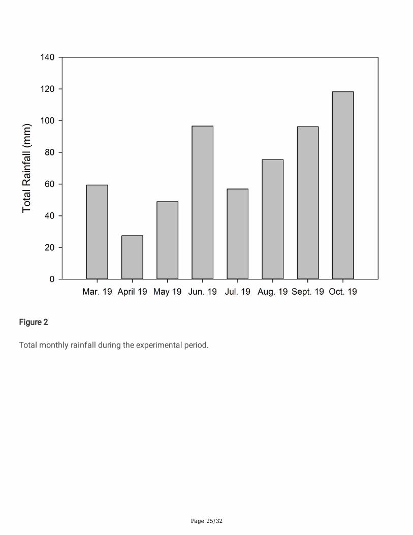
3.1 Meteorological and soil characteristics3.1.1 Rainfall patternsFigure 2 shows the total monthly rainfall during the experimental period. The total rainfall for the wholeexperimental period was 492.2 mm, and the highest rainfall event of 118.2 mm fell in October 2019.

Page 8/32

Before the highest rainfall in October, the second-highest rainfall events of 96.6 and 96.2 mm wererecorded in June and September 2019, respectively.

3.1.2 Soil variablesTable 2 presents the average soil data during the experimental period. Soil pH ranged from 5.1 ± 0.17 and5.5 ± 0.17, with the highest pH of 5.5 ± 0.17 (willow riparian buffer), which was however, not signi�cantly(LSD = 0.29) different to the grass or woodland riparian buffers. The largest soil BD of 1.2 ± 0.05 g cm− 3

was recorded in the no-buffer control, which was not signi�cantly different from the upslope maize andthe different vegetated riparian buffers (LSD = 0.19). Soil OM ranged from 9.0 ± 3.2 to 17.8 ± 2.3%, withthe largest %OM of 17.8 ± 2.3% recorded in the willow riparian buffer, which was, however, notsigni�cantly (LSD = 8.6) different to the woodland riparian buffer (15.98 ± 2.3%).

Table 2Summary of soil parameters (mean ± standard error) in the upslope maize and downslope riparian

buffers with different vegetation (upslope maize: n = 12, no-buffer control: n = 3 and each riparian buffer:n = 6) before the commencement of the current experiments in May 2019.

Parameter Upslopemaize

No-buffercontrol

GrassBuffer

Willowbuffer

WoodlandBuffer

LSD

Soil pH 5.1 ± 0.17 5.1 ± 0.19 5.4 ± 0.17

5.5 ± 0.17 5.4 ± 0.17 0.29

Bulk density (g cm− 

3)1.21 ± 0.03 1.21 ± 0.05 1.1 ± 

0.041.2 ± 0.04 1.2 ± 0.04 0.19

Organic matter (%w/w)

9.9 ± 1.3 9.0 ± 3.2 12.2 ± 2.3

17.8 ± 2.3 16.0 ± 2.3 8.6

NH4+-N (mg kg− 1

dry soil)27.4 ± 2.98 20.6 ± 4.6 6.4 ± 2.7 13.6 ± 2.7 9.1 ± 2.7 7.8

TON (mg kg− 1 drysoil)

55.7 ± 1.7 42.8 ± 3.7 13.6 ± 3.0

4.99 ± 3.0 10.9 ± 3.0 10.0

WFPS (%) 86.9 ± 5.3 81.7 ± 9.9 86.7 ± 7.2

102.9 ± 7.2

98.2 ± 7.2 18.6

3.1.3 Soil mineral N-dynamicsFigure 3 shows soil mineral N dynamics during the experimental period. At the commencement of theexperiment, NH4

+-N was < 17 mg kg− 1 dry soil in all of the treatments, with the largest of 16.7 ± 3.5 mg

kg− 1 dry soil observed in the upslope maize. However, after the second sampling event, which had beenpreceded by two fertilizer application events (Table 1), NH4

+-N increased by almost 3-fold in the no-buffercontrol and upslope maize treatments but remained relatively low in the vegetated riparian buffers.Despite the high NH4

+-N values in the no-buffer control and upslope maize crop areas after fertilization,

Page 9/32

values dropped to < 30 mg kg− 1 dry soil after the fourth sampling event and remained low until the end ofthe experimental period. The average NH4

+-N for the whole experimental period ranged from 6.4 ± 2.78 to

27.4 ± 2.8 mg kg− 1 dry soil, with the largest value of 27.4 ± 2.8 mg kg− 1 dry soil obtained from theupslope maize crop areas, which was however, not signi�cantly (LSD = 7.8) different to the no-buffercontrol. It was, however, signi�cantly different (LSD = 7.8) to the vegetated riparian buffers (Table 2).

Total oxidized N was < 30 mg kg− 1 dry soil in all of the treatments at the commencement of theexperiment (Fig. 3). However, after the second sampling event, TON increased 4-fold in the upslope maizeand no-buffer control but remained low in the riparian buffers. Despite a drop to ~ 35 mg kg− 1 dry soil inall of the upslope maize and no-buffer control areas during the �fth sampling event, the upslope maizeemerged with the highest TON of ~ 81 mg kg− 1 dry soil during the sixth sampling event. However, thesevalues dropped gradually up until the end of the experiment. Average TON for the whole experimentalperiod ranged from 4.99 ± 3.0 to 55.7 ± 1.7 mg kg− 1 dry soil, with the highest value of 55.7 ± 1.7 mg kg− 1

dry soil obtained from the upslope maize. This was signi�cantly different (LSD = 10.0) to all othertreatments, except for the no-buffer control (Table 2).

3.1.4 %WFPSSoil WFPS trends during the experimental period are shown in Fig. 4 (A), and Table 2 shows the average%WFPS for the whole season. The highest %WFPS was observed during the �fth sampling event, with theoverall highest estimate observed in the woodland riparian buffer treatment. The woodland riparianbuffer maintained higher %WFPS values than the remainder of the treatments during the experiment. Theaverage %WFPS for the whole experimental period ranged from 81.7 ± 9.9 to 102.9 ± 7.2%, with thehighest value recorded in the willow riparian buffer, which was however not signi�cantly (LSD = 18.6)different to the woodland riparian buffer treatment, or any of the other treatments.

3.3 Treatment effects on explanatory variablesTable 3 shows that soil OM differed between sampling areas; upslope and downslope chambers (P < 0.05), but there was no evidence of any other differences between treatments. Soil OM in the vegetatedriparian buffer strips was different from the upslope maize but not to the no-buffer control, which was notdifferent from the upslope maize. Soil NH4

+-N also differed between areas, but there was no evidence of

any other differences between treatments. The NH4+-N in the vegetated riparian buffer strips was

different from the upslope maize and no-buffer control, and the upslope maize and no-buffer control werenot different from each other. Soil pH was different between areas, and there was an interaction betweentreatments and the upper and lower buffer areas. The pH in the vegetated riparian buffer strips wasdifferent from the upslope maize and no-buffer control; but they were not different to each other. Soil pHwas different in the upper and lower areas of the willow and woodland riparian buffer strips but not in thegrass riparian buffer strips. TON was different between areas, but there was no evidence of any othertreatment differences. All three riparian buffer vegetation types were different, and there was no evidenceof any treatment differences for BD or WFPS (Table 2).

Page 10/32

Table 3P-values for tests from LMMs on each of the measured soil variables.

Factors and interactions OM BD NH4-N pH TON WFPS

Area 0.04 0.29 < 0.001 < 0.001 < 0.001 0.23

Area * Treatment crop 0.31 0.13 0.16 0.238 0.173 0.24

Area * Buffer area 0.551 1 0.97 0.959 0.349 0.9

Area * Treatment crop * Buffer area 0.079 1 0.77 0.05 0.5 0.84

3.4 Gas emissions

3.4.1 Gas �uxesNitrous oxide

Nitrous oxide �uxes measured during each sampling event are shown in Fig. 4 (B). The commencementof the experiment was marked by relatively low �uxes in all of the treatments. These low �uxes wereimmediately followed by the highest peak in all the treatments, observed instantly after fertilizerapplication, with the maximum mean �ux of 721.1 ± 464.3 g N2O ha− 1 day− 1 observed in the upslope

maize. There was also a smaller peak of up to 204 ± 5.7 g N2O ha− 1 day− 1 observed in the upslope maize

at around the 1st of August 2019. After that, �uxes remained < 10 g N2O ha− 1 day− 1 in all the treatments,with the upslope maize and no-buffer control maintaining predominantly higher �uxes until the end of theexperiment.

Methane

Daily CH4 �uxes, which were mostly positive and sometimes negative, are illustrated in Fig. 4 (C). Similarto N2O �uxes, the commencement of the experiment was marked by low CH4 �uxes, which increased up

to ~ 40 g CH4 ha− 1 day− 1 (in the upslope maize and no-buffer control) immediately after fertilizerapplication. After these peaks, CH4 �uxes remained low and mostly negative in all the treatments until theend of the experiment.

3.4.2 Cumulative gas emissionsNitrous oxide

There was no evidence of signi�cant treatment differences in N2O emissions between the upslope maize,no-buffer control and the three vegetated riparian buffers (p = 0.67) (Fig. 5A). Cumulative N2O emissions

had a descending order: no-buffer control; 18 929 g ha− 1 (95% con�dence intervals: 524.1–63 643 g ha− 

1) > upslope maize; 6 523 g ha− 1 (95% CI: 550.7–19 060) > woodland riparian buffer; 2 641 g ha− 1 (95%

Page 11/32

CI: -267.9-14 195 g ha− 1), willow riparian buffer; 2 324 g ha− 1 (95% CI: -382.1-13 448) > grass buffer 375g ha− 1 (95% CI: -2 340.6–7 592 g ha− 1).

Methane

The upslope maize and the no-buffer control (not signi�cantly different from each other) emittedsigni�cantly higher cumulative soil CH4 �uxes than the three vegetated riparian buffers (p = 0.02)

(Fig. 5B). Cumulative soil CH4 �uxes were in the descending order: upslope maize: 5050 ± 875 g ha− 1 >

no-buffer control: 4740 ± 1411g ha− 1 > grass riparian buffer: 3289 ± 1135 g ha− 1 > willow riparian buffer:2597 ± 1135 g ha− 1 > wood riparian buffer: -102 ± 1135 g ha− 1.

Global warming potential

Soil N2O-based GWP ranged from 1223.5 ± 362.0 (willow riparian buffer) to 10 225.1 ± 4735.7 (no buffer

control) kg CO2-Eq. ha− 1 year− 1 (Table 7). A signi�cantly the highest GWP found from the no-buffercontrol, which was, however not signi�cantly different from the upslope maize. On the other hand, soilCH4-based GWP ranged from 3.4 ± 35.9 (woodland riparian buffer) to 282.9 ± 33.4 (no buffer control) kg

CO2-Eq. ha− 1 year− 1. Despite the large GWP found in the no buffer control, it was not signi�cantlydifferent to the other treatments, but to the woodland riparian buffer. (Table 7).

Table 7Land-use effects on global warming potential (GWP)

Land-use GWP (kg CO2-C equivalent ha− 1 year− 1)

N2O CH4

Upslope maize 6181.7 ± 3545.5 ab 282.9 ± 33.4 a

No-buffer control 10225.1 ± 4735.6 a 273.8 ± 42.2 a

Grass Buffer 2518.3 ± 1689.3 bc 177.5 ± 68.1 a

Willow Buffer 1223.5 ± 362.0 c 134.7 ± 74.0 ab

Woodland Buffer 1771.3 ± 800.5 bc 3.4 ± 35.9 b

Relationships between gas emissions and measured soil variables

Table 4 and Fig. 6 show that none of the measured soil variables had a signi�cant relationship withcumulative N2O, but a slight relationship with TON (r = 0.32; p = 0.065). N2O emissions were shown to

increase with an increase in soil BD, NH4+-N, TON, and %WFPS and to decrease with an increase in pH

and OM (Fig. 7).

Page 12/32

Table 4P-values for the slope of the �tted line of the model for N2O and measured soil variables.

Variable Intercept Standard error intercept Slope Standard error slope P-value

BD -172.6 142.1 201.9 119.98 0.126

pH 122.9 191.9 -10.56 36.194 0.786

NH4 38.29 23.48 1.58 1.1513 0.18

TON 33.97 18.18 1.068 0.555 0.065

WFPS 44.16 69.45 0.2518 0.75597 0.742

OM 69.7 29.76 -0.2556 2.05029 0.902

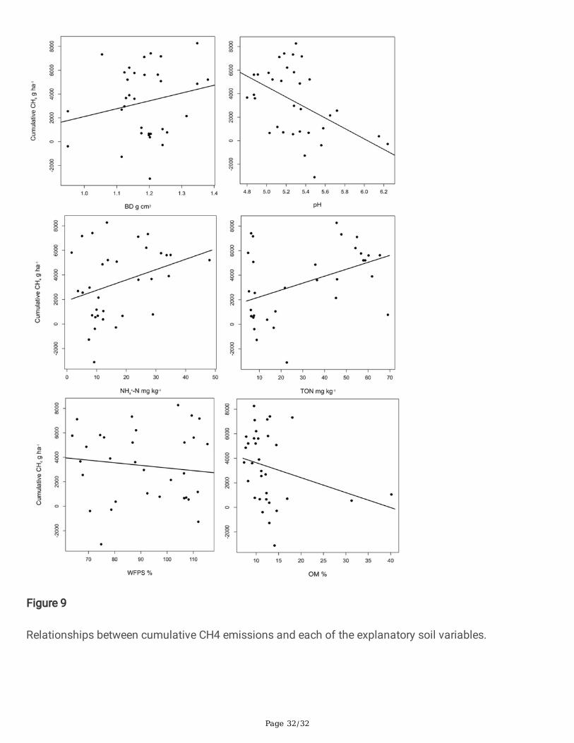
Table 5 and Fig. 8 show that pH (r = -0.44; p = 0.042), TON (r = 0.44; p = 0.005), and NH4+-N (r = 0.33; p = 

0.056) had signi�cant relationships with cumulative CH4 emissions. Soil CH4 emissions increased with

increased BD, NH4+-N, and TON and decreased with an increase in pH, %WFPS, and OM (Fig. 9).

Table 5P-values for the slope of the �tted line of the model for CH4 and measured soil variables.

Variable Intercept Standard error intercept Slope Standard error slope P-value

BD -4469 6524 6575 5467.2 0.24

pH 26829 5813 -4447 1094.7 0.042

NH4+ 1901 918.6 84.33 42.303 0.056

TON 1663 925.3 56.41 18.574 0.005

WFPS 5265 2916 -21.41 30.548 0.489

OM 4861 1197 -122 74.55 0.113

4.0 Discussion

4.1 Gas emissions

4.2.1 Soil and environmental controls of gas �uxesNitrous oxide

The largest peak N2O �ux observed in the upslope maize coincided largest %WFPS in the treatment andfollowed N fertilizer application events in the upslope maize and no buffer control (Fig. 4A and B). N2O�uxes following N fertilizer application are known to increase with increasing soil water content; mostrapidly above 70% WFPS, wherein denitri�cation is a dominant process (Abbasi and Adams, 2000; Dobbie

Page 13/32

et al., 1999; Granli and Bockman, 1994; Skiba and Ball, 2002). As one of the major drivers of N2Oproduction, soil moisture directly affects N2O production and consumption through its in�uence on the N-substrate availability, soil aeration and metabolic activity of N2O-producing microorganisms; allcontrolling the capacity of soil to produce N2O (Di et al., 2014; Khalil and Baggs, 2005; Simona et al.,2004). Fertilizer N increases soil mineral N availability; a substrate for dominant N2O microbial producingreactions; nitri�cation and denitri�cation (Butterbach-Bahl et al., 2013; Dobbie et al., 1999). Thus, thehigher �uxes were expected after fertilizer N application in the no-buffer control and the upslope maize ofthe current study, similar to other studies; particularly Halvorson et al. (2008) and Van Groenigen et al.(2004), who reported that soil N2O emissions increased linearly with increasing fertilizer N. This was

further attested to by an increase in N2O emissions with every increase in soil TON and NH4+-N (Fig. 7).

This was also in agreement with previous work, particularly Mosier (1994), Mosier et al. (1996), andBarton and Schipper (2001). Notably, the woodland and willow riparian buffers had the highest %WFPSbut were characterised by lower N2O emissions during the peak �ux. On top of the low N substrate due tothe fact that the riparian buffers were not fertilized, this could have been due to reduced diffusion in thehigh soil moisture causing a further reduction of N2O to N2 (Balaine et al., 2013; Hamonts et al., 2013). Onthe other hand, the no-buffer control and upslope maize had larger �uxes; which further highlights theinteractive role of soil moisture and mineral N in enhanced N2O production (Klemedtsson et al., 1988).The no buffer control emitted 15.6% while the upslope maize 5.4%, which means that of the total fertilizerN added, 21% was lost as N2O in the 6 month experimental period. We however, did not use stableisotopes to ascertain this.

Methane

The overall positive CH4 emissions from all treatments are most likely the result of the high %WFPS

experienced during most of the experimental period. The upper values (~ 5 kg CH4 ha− 1) are similar tothose reported by Groh et al. (2015). A number of �eld investigations have identi�ed soil water content asone of the critical controls of CH4 production and consumption in soils from different ecosystems (Khaliland Baggs, 2005; Kim et al., 2010; Wu et al., 2010). Similarly, in our study, the peak CH4 �uxes followedimmediately after the highest %WFPS (Fig. 4C). High soil moisture contents are documented drivers ofCH4 production and emissions in soils; as a group of strictly anaerobic bacteria biologically produce amajority of CH4 in reduced environments (Ehhalt et al., 2001; Ehhalt and Schmidt, 1978; Yang and Chang,1998). Soil moisture directly affects the production of soil CH4 through its in�uence on C-substrateavailability, soil aeration, and metabolic activity of CH4 producing microorganisms; all affecting thecapacity of soil to produce or consume CH4 (Khalil and Baggs, 2005; Simona et al., 2004). Further, therole of soil moisture in CH4 production and subsequent emissions was attested to by the low (sometimesnegative) CH4 �uxes we observed; coinciding with low soil %WFPS at the end of August (Fig. 4); similar to(Luo et al., 2013). The latter work observed that soil moisture affected soil CH4 consumption through its

Page 14/32

effect on substrate availability and redistribution, soil aeration, and the metabolic activity ofmicroorganisms.

4.1.2 Gas emissions in upslope maize and downsloperiparian buffer stripsNitrous oxide

For a riparian buffer to be considered an atmospheric concern, it must emit more N2O than the cropland itserves (Fisher et al., 2014). In the current study, the no-buffer control proved to be an atmosphericconcern, since it generated the highest N2O emissions compared to the upslope maize and the three

vegetated riparian buffers (Fig. 5A). The maximum cumulative emissions of 20 kg N2O (~ 12 kg N ha− 1)are similar to Kim et al. (2009) (2-year study) and Groh et al. (2015) (1-year study), who observed 24 and14.8 kg N2O ha− 1, respectively, in maize in a Humid Continental climate. The high N2O emissionsobserved in the no-buffer control could have been due to applied fertilizer N (particularly readily availableinorganic N); which increased mineral N availability for the N2O-producing nitri�cation and denitri�cationprocesses, similar to the responses reported by other authors; particularly Dobbie et al. (1999) and(Butterbach-Bahl et al., 2013). In fact, the high N2O emissions in the no-buffer control shows a downwardmovement of the fertilizer applied N with rainwater. This was further attested to by the high mineral N(TON and NH4

+) in the no-buffer control compared to the remainder of the treatments (Table 2) and anincrease in N2O emissions with every increase in mineral N (Fig. 8). The fact that the vegetated riparianbuffers had low N2O emissions shows that they served their purpose of intercepting and processing N toN2 through denitri�cation induced by their high soil moisture (Groffman et al., 1991; Knowles, 1982)before it was delivered off-site. Interestingly, the riparian buffers had ideal condition to promote fulldenitri�cation, reducing N to N2, especially at the high moisture and in the case of willow and woodlandthe high organic matter and potentially available C which explains their low N2O compared to the upslopepasture and no buffer control. The low N2O emissions in the vegetated riparian buffers could also be aresult of the fact that the riparian buffer strips were not directly fertilized; further highlighting the role offertilizer N in increasing mineral N availability for N2O producing processes; similar to Davis et al. (2019),Hefting et al. (2003) and Iqbal et al. (2015). The second-highest N2O emissions observed in the upslopemaize could have also been due to the N fertilizer applied.

Methane

The fact that the upslope maize and no-buffer control treatments exhibited high CH4 emissions may have

been a result of NH4+-N based fertilizer N applied in the two treatments, since NH4

+-N has been shown toinhibit CH4 oxidation (Hütsch, 1998; Kravchenko et al., 2002; Tlustos et al., 1998); which often results in anet increase in CH4 emitted from soil (Bronson and Mosier, 1994). This inhibition is thought to be either ageneral salt effect (Gulledge and Schimel, 1998), a competition between ammonia (NH3) and CH4 formethane monooxygenase enzymes (Bédard and Knowles, 1989), or non-competitive inhibition by

Page 15/32

hydroxylamine (NH2OH) or nitrite (NO2−) produced during NH3 oxidation (King and Schnell, 1994). To

further emphasize the role of mineral N in inhibiting CH4 oxidation, the three vegetated and unfertilizedriparian buffers had signi�cantly lower CH4 emissions than the upslope maize and the no-buffer control(Fig. 5).

4.1.3 Global warming potentialsThe high N2O and CH4-based GWP observed in the no buffer control shows that growing a maize cropwithout implementing riparian buffer vegetation may increase the risk of global warming potential. On apositive note, implementing the willow and woodland riparian buffers in tandem with a maize crop mayreduce the risk of global warming potential while addressing water quality problems they are usuallyimplemented for.

4.2 Implications of the �ndingsOur �ndings have a number of implications especially in research and environmental policy. Althoughriparian buffer strips are conventionally implemented to help tackle the widespread water quality issuesin the UK, and elsewhere globally, associated with intensive farming, our work demonstrates the co-bene�ts of their uptake for gaseous emissions. Many countries globally are focussing on the urgent needto tackle the climate emergency and robust evidence on the e�cacy of interventions for reducing harmfulgaseous emissions is critical for engaging stakeholders including farmers.

The �ndings of the current study also have implications for the calibration of process-based models tosimulate N2O and CH4 emissions from croplands and/ or riparian buffer areas with varying vegetation,which has been challenging in the past due to lack of data availability. Process-based models includingthe Riparian Ecosystem Management Model (REMM) (Lowrance et al., 2000)have been calibrated tosimulate soil processes under riparian buffers. For example, REMM has been used to simulategroundwater movement, water table depths, surface runoff and annual hydrological budgets (Inamdar etal., 1999b) and N, phosphorus (P), and C cycling (Dukes and Evans, 2003; Inamdar et al., 1999a)interactions between varying riparian buffer systems. Other watershed models, such as the Soil andWater Assessment Tool (SWAT), have been calibrated to assess the effectiveness of riparian buffers forreducing total organic N in a watershed (Lee et al., 2020). A landscape model, the Morgan-Morgan-Finneytopographic wetness index (MMF-TWI), has been calibrated to simulate erosion reduction using riparianbuffers (Smith et al., 2018a). But, to the best of our knowledge, none of these mechanistic models havebeen calibrated to simulate N2O and CH4 emissions from riparian buffers and further compared withemissions from croplands. Whilst some process-based models, e.g., Denitri�cation-Decomposition(DNDC), has been calibrated to simulate biogeochemical cycles including N2O emissions from differentgrass riparian buffers in Illinois, USA (Gopalakrishnan et al., 2012), to the best of our knowledge, we arenot aware of this model having being calibrated to simulate GHG emissions from riparian buffers in theUK.

4.3 Limitations of the study

Page 16/32

One of the signi�cant limitations of the current study is that it was based on a replicated plot-scaleexperimental facility. This means that our results represent the climate, soil, and environmentalconditions prevailing at the experimental site at North Wyke, Devon, UK. Similar conditions in terms ofannual rainfall, soils and farming system, are present in 1843 km2 of farmed land across England(Collins et al., 2021). Our results provide robust data on short-term N and C gaseous emissions andclearly, longer-term measurements would help in con�rming our �ndings. Although the static chamber ischeaper and easy to use, further shortcoming may be associated with it as it was used to trap the gasesin the �eld for the current experiment. For instance Healy et al. (1996) and Rochette (2011) reported thatinsertion of chambers into the soil may limit lateral gas exchange. However, Rochette (2011) suggestedthat such limitations may be overcome by inserting the chamber collars prior to chamber use. But, thesame author argued that this practice may affect soil temperature by shading the soil and affect soilmoisture by preventing soil run-off as well as affect gas exchange through formation of shrinkage cracksat the collar-soil interface.

5.0 ConclusionsOur replicated plot-scale facility experiment showed that the N-fertilized no-buffer control and upslopeareas used for maize cropping might be signi�cant N2O and CH4 sources, respectively. Furthermore, thelow N2O and CH4-based GWP from the willow and woodland riparian buffers show that the willow maymitigate global warming potential when implemented for water quality protection purposes in maizeproduction. Accordingly, our results attest to the unintended bene�ts of riparian buffers for reducinggaseous emissions, despite primarily being implemented as water quality protection measures. The typeof work undertaken in our experiment herein demonstrates the importance of gathering data for co-bene�ts and trade-offs associated with the management of agroecosystems.

DeclarationsFunding: The Department of Higher Education and Training (New Generation Gap of AcademicsProgram) and National Research Foundation-Thuthuka (Grant Number: 117964), both under the SouthAfrican government, are acknowledged for �nancially supporting this study. The work was also facilitatedby the UKRI (UK Research and Innovation) Biotechnology and Biological Sciences Research Council(BBSRC) via grant (awarded to ALC) BB/N004248/1 - “Impacts of different vegetation in riparian bufferstrips on hydrology and water quality”. The British Council is acknowledged for a Researcher Links TravelGrant (2017-RLTG9-1069) that initiated the collaboration between J. Dlamini and Rothamsted Research.Rothamsted Research is supported by strategic funding from UKRI-BBSRC via its Institute StrategicProgrammes, including BBS/E/C/000I0320 and BBS/E/C/000I0330.  

Data availability: Data available from authors on request

Code availability: Not Applicable

Page 17/32

Code availability: Not applicable

Ethical approval: Not applicable

Consent to participate: Not applicable

Consent for publication: Not applicable

Con�icts of interest/Competing interests: Authors declared no con�icts of interest

References1. Abbasi M, Adams W (2000) Estimation of simultaneous nitri�cation and denitri�cation in grassland

soil associated with urea-N using 15N and nitri�cation inhibitor. Biol Fertil Soils 31:38–44

2. Amirinejad AA, Kamble K, Aggarwal P, Chakraborty D, Pradhan S, Mittal RB (2011) Assessment andmapping of spatial variation of soil physical health in a farm. Geoderma 160:292–303

3. Armstrong AC, Garwood E (1991) Hydrological consequences of arti�cial drainage of grassland.Hydrol Process 5:157–174. DOI:https://doi.org/10.1002/hyp.3360050204

4. Aronsson P, Perttu K (2001) Willow vegetation �lters for wastewater treatment and soil remediationcombined with biomass production. For Chron 77:293–299

5. Balaine N, Clough TJ, Beare MH, Thomas SM, Meenken ED, Ross JG (2013) Changes in relative gasdiffusivity explain soil nitrous oxide �ux dynamics. Soil Sci Soc Am J 77:1496–1505.DOI:https://doi.org/10.2136/sssaj2013.04.0141

�. Ball BC, Scott A, Parker JP (1999) Field N2O, CO2 and CH4 �uxes in relation to tillage, compaction andsoil quality in Scotland. Soil Tillage Res 53:29–39. DOI:https://doi.org/10.1016/S0167-1987(99)00074-4

7. Barton L, Schipper L (2001) Regulation of nitrous oxide emissions from soils irrigated with dairyfarm e�uent. J Environ Qual 30:1881–1887. DOI:https://doi.org/10.2134/jeq2001.1881

�. Bechmann ME, Bøe F (2021) Soil tillage and crop growth effects on surface and subsurface runoff,loss of soil, phosphorus and nitrogen in a cold climate. Land 10:77

9. Bédard C, Knowles R (1989) Physiology, biochemistry, and speci�c inhibitors of CH4, NH4+, and CO

oxidation by methanotrophs and nitri�ers. Microbiol Rev 53:68–84.DOI:https://doi.org/10.1128/mr.53.1.68-84.1989

10. Bowden WB (1986) Gaseous nitrogen emmissions from undisturbed terrestrial ecosystems: Anassessment of their impacts on local and global nitrogen budgets. Biogeochemistry 2:249–279

11. Bronson K, Mosier A (1994) Suppression of methane oxidation in aerobic soil by nitrogen fertilizers,nitri�cation inhibitors, and urease inhibitors. Biol Fertil Soils 17:263–268

12. Butterbach-Bahl K, Baggs EM, Dannenmann M, Kiese R, Zechmeister-Boltenstern S (2013) Nitrousoxide emissions from soils: how well do we understand the processes and their controls? Philos

Page 18/32

Trans R Soc Lond B Biol Sci 368:20130122. DOI:https://doi.org/10.1098/rstb.2013.0122

13. Chadwick D, Cardenas L, Misselbrook T, Smith K, Rees R, Watson C, McGeough K, Williams J, Cloy J,Thorman R (2014) Optimizing chamber methods for measuring nitrous oxide emissions from plot-based agricultural experiments. Eur J Soil Sci 65:295–307

14. Clayden B, Hollis JM (1985) Criteria for differentiating soil series, Tech Monograph 17, Harpenden,UK

15. Collins A, Zhang Y, Upadhayay H, Pulley S, Granger S, Harris P, Sint H, Gri�th B (2021) Currentadvisory interventions for grazing ruminant farming cannot close exceedance of modern backgroundsediment loss–Assessment using an instrumented farm platform and modelled scaling out. EnvironSci Policy 116:114–127. DOI:https://doi.org/10.1016/j.envsci.2020.11.004

1�. Conen F, Smith K (2000) An explanation of linear increases in gas concentration under closedchambers used to measure gas exchange between soil and the atmosphere. Eur J Soil Sci 51:111–117

17. Conrad R (2007) Microbial ecology of methanogens and methanotrophs. Adv Agron 96:1–63.DOI:https://doi.org/10.1016/S0065-2113(07)96005-8

1�. Davidson EA (2009) Microbial processes of production and consumption of nitric oxide, nitrousoxide and methane. In: Matson PA, HArris RC (eds) Biogenic Trace Gases: Measuring Emisions fromSoil and Water. Wiley-Blackwell, Oxford

19. Davis MP, Groh TA, Jaynes DB, Parkin TB, Isenhart TM (2019) Nitrous oxide emissions fromsaturated riparian buffers: Are we trading a water quality problem for an air quality problem? JEnviron Qual 48:261–269. DOI:https://doi.org/10.2134/jeq2018.03.0127

20. De Klein C, Harvey M (2012) Nitrous oxide chamber methodology guidelines. In: Global ResearchAlliance on Agricultural Greenhouse Gases. Wellington, New Zealand, Ministry for Primary Industries

21. DEFRA (2019) The guide to cross compliance in England 2019, in: F. a. R. A. Department forEnvironment (Ed.), United Kingdom

22. Del Grosso S, Walsh M, Du�eld J (2008) US agriculture and forestry greenhouse gas inventory:1990–2005. USDA Technical Bulletin, Washington, DC, USA

23. Di HJ, Cameron KC, Podolyan A, Robinson A (2014) Effect of soil moisture status and a nitri�cationinhibitor, dicyandiamide, on ammonia oxidizer and denitri�er growth and nitrous oxide emissions in agrassland soil. Soil Biol Biochem 73:59–68. DOI:https://doi.org/10.1016/j.soilbio.2014.02.011

24. Dobbie K, McTaggart IP, Smith K (1999) Nitrous oxide emissions from intensive agricultural systems:variations between crops and seasons, key driving variables, and mean emission factors. Journal ofGeophysical Research: Atmospheres 104:26891–26899

25. Dukes M, Evans R (2003) Riparian ecosystem management model: Hydrology performance andsensitivity in the North Carolina middle coastal plain. Trans ASABE 46:1567.doi:10.13031/2013.15645. DOI

Page 19/32

2�. Dutaur L, Verchot LV (2007) A global inventory of the soil CH4 sink. Global Biogeochem Cycles 21.DOI: https://doi.org/10.1029/2006GB002734

27. Ehhalt D, Prather M, Dentener F, Derwent R, Dlugokencky EJ, Holland E, Isaksen I, Katima J, KirchhoffV, Matson P (2001) Atmospheric chemistry and greenhouse gases. Paci�c Northwest National Lab.(PNNL), Richland, WA (United States)

2�. Ehhalt D, Schmidt U (1978) Sources and sinks of atmospheric methane. Pure Appl Geophys116:452–464

29. FAO (2006) Guidelines for soil description Rome. Food and Agricultural Organisation of the UnitedNations, Italy

30. Firestone M (1982) Biological denitri�cation, In: Stevenson F (ed), Nitrogen in agricultural soils,American Society of Agronomy, Inc. Crop Science Society of America, Inc. Soil Science Society ofAmerica Inc., Madison. pp 289–326

31. Fisher K, Jacinthe P, Vidon P, Liu X, Baker M (2014) Nitrous oxide emission from cropland andadjacent riparian buffers in contrasting hydrogeomorphic settings. J Environ Qual 43:338–348.DOI:https://doi.org/10.2134/jeq2013.06.0223

32. Friedel J, Munch J, Fischer W (1996) Soil microbial properties and the assessment of available soilorganic matter in a haplic luvisol after several years of different cultivation and crop rotation. SoilBiol Biochem 28:479–488. DOI:https://doi.org/10.1016/0038-0717(95)00188-3

33. Gopalakrishnan G, Cristina Negri M, Salas W (2012) Modeling biogeochemical impacts of bioenergybuffers with perennial grasses for a row-crop �eld in Illinois. GCB Bioenergy 4:739–750.DOI:https://doi.org/10.1111/j.1757-1707.2011.01145.x

34. Grandy AS, Loecke TD, Parr S, Robertson GP (2006) Long-term trends in nitrous oxide emissions, soilnitrogen, and crop yields of till and no-till cropping systems. J Environ Qual 35:1487–1495

35. Granli T, Bockman OC (1994) Nitrous oxide from agriculture. Norwegian Journal of AgriculturalSciences 12:94–128

3�. Groffman PM, Axelrod EA, Lemunyon JL, Sullivan WM (1991) Denitri�cation in grass and forestvegetated �lter strips. J Environ Qual 20:671–674

37. Groh TA, Gentry LE, David MB (2015) Nitrogen removal and greenhouse gas emissions fromconstructed wetlands receiving tile drainage water. J Environ Qual 44:1001–1010

3�. Gronle A, Lux G, Böhm H, Schmidtke K, Wild M, Demmel M, Brandhuber R, Wilbois K-P, Heß J (2015)Effect of ploughing depth and mechanical soil loading on soil physical properties, weed infestation,yield performance and grain quality in sole and intercrops of pea and oat in organic farming. SoilTillage Res 148:59–73. DOI:https://doi.org/10.1016/j.still.2014.12.004

39. Gulledge J, Schimel JP (1998) Moisture control over atmospheric CH4 consumption and CO2

production in diverse Alaskan soils. Soil Biol Biochem 30:1127–1132.DOI:https://doi.org/10.1016/S0038-0717(97)00209-5

Page 20/32

40. Halvorson AD, Del Grosso SJ, Reule CA (2008) Nitrogen, tillage, and crop rotation effects on nitrousoxide emissions from irrigated cropping systems. J Environ Qual 37:1337–1344.DOI:https://doi.org/10.2134/jeq2007.0268

41. Hamonts K, Balaine N, Moltchanova E, Beare M, Thomas S, Wakelin SA, O'Callaghan M, Condron LM,Clough TJ (2013) In�uence of soil bulk density and matric potential on microbial dynamics,inorganic N transformations, N2O and N2 �uxes following urea deposition. Soil Biol Biochem 65:1–11. DOI:https://doi.org/10.1016/j.soilbio.2013.05.006

42. Healy RW, Striegl RG, Russell TF, Hutchinson GL, Livingston GP (1996) Numerical Evaluation ofStatic-Chamber Measurements of Soil—Atmosphere Gas Exchange: Identi�cation of PhysicalProcesses. Soil Sci Soc Am J 60:740–747.DOI:https://doi.org/10.2136/sssaj1996.03615995006000030009x

43. Hefting MM, Bobbink R, de Caluwe H (2003) Nitrous oxide emission and denitri�cation in chronicallynitrate-loaded riparian buffer zones. J Environ Qual 32:1194–1203

44. Hütsch B (1998) Methane oxidation in arable soil as inhibited by ammonium, nitrite, and organicmanure with respect to soil pH. Biol Fertil Soils 28:27–35.DOI:https://doi.org/10.1007/s003740050459

45. Inamdar S, Lowrance R, Altier L, Williams R, Hubbard R (1999a) Riparian Ecosystem ManagementModel (REMM): II. Testing of the water quality and nutrient cycling component for a coastal plainriparian system. Trans ASABE 42:1691

4�. Inamdar S, Sheridan J, Williams R, Bosch D, Lowrance R, Altier L, Thomas D (1999b) Riparianecosystem management model (REMM): I. Testing of the hydrologic component for a coastal plainriparian system. Trans ASABE 42:1679

47. IPCC (2006) 2006 IPCC guidelines for national greenhouse gas inventories Institute for GlobalEnvironmental Strategies Hayama, Japan

4�. IPCC (2008) IPCC, 2007: climate change 2007: synthesis report. IPCC

49. IPCC (2014) Climate change 2014: synthesis report. Contribution of Working Groups I, II and III to the�fth assessment report of the Intergovernmental Panel on Climate Change IPCC

50. Iqbal J, Parkin TB, Helmers MJ, Zhou X, Castellano MJ (2015) Denitri�cation and nitrous oxideemissions in annual croplands, perennial grass buffers, and restored perennial grasslands. Soil SciSoc Am J 79:239–250. DOI:10.2136/sssaj2014.05.0221

51. Jacinthe P-A, Vidon P, Fisher K, Liu X, Baker M (2015) Soil methane and carbon dioxide �uxes fromcropland and riparian buffers in different hydrogeomorphic settings. J Environ Qual 44:1080–1090.DOI:https://doi.org/10.2134/jeq2015.01.0014

52. Jacinthe P, Bills J, Tedesco L, Barr R (2012) Nitrous oxide emission from riparian buffers in relation tovegetation and �ood frequency. J Environ Qual 41:95–105.DOI:https://doi.org/10.2134/jeq2011.0308

53. Kaiser E-A, Munch JC, Heinemeyer O (1996) Importance of soil cover box area for the determinationof N2O emissions from arable soils. Plant Soil 181:185–192.

Page 21/32

DOI:https://doi.org/10.1007/BF00012052

54. Khalil M, Baggs E (2005) CH4 oxidation and N2O emissions at varied soil water-�lled pore spacesand headspace CH4 concentrations. Soil Biol Biochem 37:1785–1794.DOI:https://doi.org/10.1016/j.soilbio.2005.02.012

55. Kim D-G, Isenhart TM, Parkin TB, Schultz RC, Loynachan TE (2010) Methane �ux in cropland andadjacent riparian buffers with different vegetation covers. J Environ Qual 39:97–105.DOI:10.2134/jeq2008.0408

5�. Kim D, Isenhart TM, Parkin TB, Schultz RC, Loynachan TE, Raich JW (2009) Nitrous oxide emissionsfrom riparian forest buffers, warm-season and cool-season grass �lters, and crop �elds. BiogeosciDiscuss 6:607

57. King GM, Schnell S (1994) Ammonium and nitrite inhibition of methane oxidation by Methylobacteralbus BG8 and Methylosinus trichosporium OB3b at low methane concentrations. Appl EnvironMicrobiol 60:3508–3513

5�. Klemedtsson L, Svensson B, Rosswall T (1988) Relationships between soil moisture content andnitrous oxide production during nitri�cation and denitri�cation. Biol Fertil Soils 6:106–111.DOI:https://doi.org/10.1007/BF00257658

59. Knowles R (1982) Denitri�cation. Microbiol Rev 46:43

�0. Kravchenko I, Boeckx P, Galchenko V, Van Cleemput O (2002) Short-and medium-term effects of NH4+

on CH4 and N2O �uxes in arable soils with a different texture. Soil Biol Biochem 34:669–678.DOI:https://doi.org/10.1016/S0038-0717(01)00232-2

�1. Lane A (1997) The UK environmental change network database: An integrated information resourcefor long-term monitoring and research. J Environ Manage 51:87–105

�2. Le Mer J, Roger P (2001) Production, oxidation, emission and consumption of methane by soils: areview. Eur J Soil Biol 37:25–50

�3. Lee S, McCarty GW, Moglen GE, Li X, Wallace CW (2020) Assessing the effectiveness of riparianbuffers for reducing organic nitrogen loads in the Coastal Plain of the Chesapeake Bay watershedusing a watershed model. J Hydrol 585:124779. DOI:https://doi.org/10.1016/j.jhydrol.2020.124779

�4. Livingston G, Hutchinson G (1995) Enclosure-based measurement of trace gas exchange:applications and sources of error. In: Matson P, Harris RC (eds) Biogenic Trace Gases: MeasuringEmissions from Soil and Water. Blackwell Publishing, Massachusetts, pp 14–51

�5. Lowrance R, Altier L, Williams R, Inamdar S, Sheridan J, Bosch D, Hubbard R, Thomas D (2000)REMM: The riparian ecosystem management model. J Soil Water Conserv 55:27–34

��. Luo G, Kiese R, Wolf B, Butterbach-Bahl K (2013) Effects of soil temperature and moisture onmethane uptake and nitrous oxide emissions across three different ecosystem types. Biogeosciences10:3205–3219. DOI:https://doi.org/10.5194/bg-10-3205-2013

�7. Macleod CJA, Humphreys MW, Whalley WR, Turner L, Binley A, Watts CW, Skøt L, Joynes A, HawkinsS, King IP, O'Donovan S, Haygarth PM (2013) A novel grass hybrid to reduce �ood generation in

Page 22/32

temperate regions. Sci Rep 3:1683. DOI:10.1038/srep01683

��. Megonigal JP, Guenther AB (2008) Methane emissions from upland forest soils and vegetation. TreePhysiol 28:491–498. DOI:https://doi.org/10.1093/treephys/28.4.491

�9. Mosier A (1994) Nitrous oxide emissions from agricultural soils. Fertilizer Research 37:191–200.DOI:https://doi.org/10.1007/BF00748937

70. Mosier A, Duxbury J, Freney J, Heinemeyer O, Minami K (1996) Nitrous oxide emissions fromagricultural �elds: Assessment, measurement and mitigation, Progress in Nitrogen Cycling Studies,Springer. pp. 589–602

71. Müller C, Stevens R, Laughlin R, Jäger H-J (2004) Microbial processes and the site of N2O productionin a temperate grassland soil. Soil Biol Biochem 36:453–461

72. Neugschwandtner R, Liebhard P, Kaul H, Wagentristl H (2014) Soil chemical properties as affected bytillage and crop rotation in a long-term �eld experiment. Plant Soil Environ 60:57–62

73. Orr R, Murray P, Eyles C, Blackwell M, Cardenas L, Collins A, Dungait J, Goulding K, Gri�th B, Gurr S(2016) The NorthWyke Farm Platform: effect of temperate grassland farming systems on soilmoisture contents, runoff and associated water quality dynamics. Eur J Soil Sci 67:374–385

74. Ouattara K, Ouattara B, Assa A, Sédogo PM (2006) Long-term effect of ploughing, and organicmatter input on soil moisture characteristics of a Ferric Lixisol in Burkina Faso. Soil Tillage Res88:217–224. DOI:https://doi.org/10.1016/j.still.2005.06.003

75. Poulton P, Johnston J, Macdonald A, White R, Powlson D (2018) Major limitations to achieving “4 per1000” increases in soil organic carbon stock in temperate regions: Evidence from long-termexperiments at Rothamsted Research, United Kingdom. Glob Change Biol 24:2563–2584

7�. Ramaswamy V, Boucher O, Haigh J, Hauglustine D, Haywood J, Myhre G, Nakajima T, Shi G, SolomonS (2001) Radiative forcing of climate. Clim Change 349

77. Reinsch T, Loges R, Kluß C, Taube F (2018) Renovation and conversion of permanent grass-cloverswards to pasture or crops: Effects on annual N2O emissions in the year after ploughing. Soil TillageRes 175:119–129. DOI:https://doi.org/10.1016/j.still.2017.08.009

7�. Rennie S, Andrews C, Atkinson S, Beaumont D, Benham S, Bowmaker V, Dick J, Dodd B, McKenna C,Pallett D (2020) The UK Environmental Change Network datasets–integrated and co-located data forlong-term environmental research (1993–2015). Earth Syst Sci Data 12:87–107

79. Rochette P (2011) Towards a standard non-steady-state chamber methodology for measuring soilN2O emissions. Anim Feed Sci Technol 166:141–146

�0. Shen Y, McLaughlin N, Zhang X, Xu M, Liang A (2018) Effect of tillage and crop residue on soiltemperature following planting for a Black soil in Northeast China. Sci Rep 8:1–9.DOI:https://doi.org/10.1038/s41598-018-22822-8

�1. Simona C, Ariangelo DPR, John G, Nina N, Ruben M, Jose SJ (2004) Nitrous oxide and methane�uxes from soils of the Orinoco savanna under different land uses. Glob Change Biol 10:1947–1960.DOI:https://doi.org/10.1111/j.1365-2486.2004.00871.x

Page 23/32

�2. Skiba U, Ball B (2002) The effect of soil texture and soil drainage on emissions of nitric oxide andnitrous oxide. Soil Use Manag 18:56–60

�3. Smith HG, Peñuela A, Sangster H, Sellami H, Boyle J, Chiverrell R, Schillereff D, Riley M (2018a)Simulating a century of soil erosion for agricultural catchment management. Earth Surf ProcessLandf 43:2089–2105. DOI:https://doi.org/10.1002/esp.4375

�4. Smith K, Ball T, Conen F, Dobbie K, Massheder J, Rey A (2018b) Exchange of greenhouse gasesbetween soil and atmosphere: interactions of soil physical factors and biological processes. Eur JSoil Sci 69:10–20

�5. Smith K, Dobbie K, Ball B, Bakken L, Sitaula B, Hansen S, Brumme R, Borken W, Christensen S, PrieméA (2000) Oxidation of atmospheric methane in Northern European soils, comparison with otherecosystems, and uncertainties in the global terrestrial sink. Glob Change Biol 6:791–803

��. Stehfest E, Bouwman L (2006) N2O and NO emission from agricultural �elds and soils under naturalvegetation: summarizing available measurement data and modeling of global annual emissions.Nutr Cycling Agroecosyst 74:207–228

�7. Sydes C, Grime J (1981) Effects of tree leaf litter on herbaceous vegetation in deciduous woodland: I.Field investigations. J Ecol:237–248

��. Tlustos P, Willison T, Baker J, Murphy D, Pavlikova D, Goulding K, Powlson D (1998) Short-termeffects of nitrogen on methane oxidation in soils. Biol Fertil Soils 28:64–70.DOI:https://doi.org/10.1007/s003740050464

�9. Ulén B (1997) Nutrient losses by surface run-off from soils with winter cover crops and spring-ploughed soils in the south of Sweden. Soil Tillage Res 44:165–177.DOI:https://doi.org/10.1016/S0167-1987(97)00051-2

90. Van Groenigen J, Kasper vG, Velthof G, Van den Pol-van Dasselaar A, Kuikman P (2004) Nitrousoxide emissions from silage maize �elds under different mineral nitrogen fertilizer and slurryapplications. Plant Soil 263:101–111. DOI:https://doi.org/10.1023/B:PLSO.0000047729.43185.46

91. Wang Q, Bai Y, Gao H, He J, Chen H, Chesney R, Kuhn N, Li H (2008) Soil chemical properties andmicrobial biomass after 16 years of no-tillage farming on the Loess Plateau, China. Geoderma144:502–508

92. Wilke B-M (2005) Determination of chemical and physical soil properties. In: Varma A (ed)Monitoring and assessing soil bioremediation. Springer, Berlin Heidelberg, pp 47–95

93. Wu X, Yao Z, Brüggemann N, Shen Z, Wolf B, Dannenmann M, Zheng X, Butterbach-Bahl K (2010)Effects of soil moisture and temperature on CO2 and CH4 soil–atmosphere exchange of variousland use/cover types in a semi-arid grassland in Inner Mongolia, China. Soil Biol Biochem 42:773–787

94. Yamulki S, Jarvis S (2002) Short-term effects of tillage and compaction on nitrous oxide, nitric oxide,nitrogen dioxide, methane and carbon dioxide �uxes from grassland. Biol Fertil Soils 36:224–231

95. Yang S-S, Chang H-L (1998) Effect of environmental conditions on methane production andemission from paddy soil. Agric Ecosyst Environ 69:69–80

Page 24/32

9�. Yao P, Li X, Nan W, Li X, Zhang H, Shen Y, Li S, Yue S (2017) Carbon dioxide �uxes in soil pro�les asaffected by maize phenology and nitrogen fertilization in the semiarid Loess Plateau. Agric EcosystEnviron 236:120–133

97. Zhang T, Huang X, Yang Y, Li Y, Dahlgren RA (2016) Spatial and temporal variability in nitrous oxideand methane emissions in urban riparian zones of the Pearl River Delta. Environ Sci Pollut Res23:1552–1564

Figures

Figure 1

A schematic diagram of the replicated experimental plots and their location at NorthWyke, UnitedKingdom.

Page 25/32

Figure 2

Total monthly rainfall during the experimental period.

Page 26/32

Figure 3

Soil NH4+ and TON in the upslope maize and downslope riparian buffers during the experimental period.

Page 27/32

Figure 4

Daily (A) soil WFPS, and (B) N2O, and (C) CH4 �uxes in the upslope maize and downslope riparianbuffers. Data points and error bars represent the treatment means (cropland: n = 12, no-buffer control: n =3, grass, woodland and willow buffer: n = 6) and SE during each sampling day. The vertical line in CH4marks 0 �uxes.

Page 28/32

Figure 5

Cumulative (A) N2O and (B) CH4 emissions for the whole experimental period from the upslope maizeand different downslope buffer vegetation. Error bars represent 95% con�dence intervals (cropland: n =12, no-buffer control: n = 3, grass, woodland and willow buffer: n = 6). Vertical lines are 95% con�denceintervals.

Page 29/32

Figure 6

Scatterplot showing the relationships between the variables pH, soil NH4+-N, soil TON, water �lled porespace (WFPS%), organic matter (OM), bulk density (BD) and cumulative N2O emissions for the upslopemaize and the downslope riparian buffers with different vegetation treatments. r = Pearson’s correlationcoe�cient.

Page 30/32

Figure 7

Relationships between cumulative N2O emissions and each of the explanatory soil variables.

Page 31/32

Figure 8

Scatterplot showing the relationships between the variables pH, soil NH4+-N, soil TON, water �lled porespace (WFPS%), organic matter (OM), bulk density (BD) and cumulative CH4 emissions for the upslopemaize and the downslope riparian buffers with different vegetation treatments. r = Pearson’s correlationcoe�cient.

Page 32/32

Figure 9

Relationships between cumulative CH4 emissions and each of the explanatory soil variables.