OF COLLEGE · OF COLLEGE \liDIIIAlI A VInUIlmlM POLYTECHNIC I~STITUTE UMIVERSITY AND STATE mnlk I I ... Aidpi + i+l + Ai-l'pi-1 +. . . = continuity error, each control volume

$Page 1: OF COLLEGE · OF COLLEGE \liDIIIAlI A VInUIlmlM POLYTECHNIC I~STITUTE UMIVERSITY AND STATE mnlk I I ... Aidpi + i+l + Ai-l'pi-1 +. . . = continuity error, each control volume$
OF COLLEGE

\ l i D I I I A l I A V I n U I l m l M

POLYTECHNIC I~STITUTE

UMIVERSITY

AND STATE mnlk

I I 'BLACKSBURG, VIRGINIA

https://ntrs.nasa.gov/search.jsp?R=19870014492 2019-02-11T04:24:02+00:00Z

I I I I i I I 1 I I I 1 I I I I I 1 I

Final Report on NASA Grant No. NAG 3-593 Thermodynamic Evaluation of Transonic Compressor Rotors

Using the Finite Volume Approach f o r the period

12/20/84 - 12/19/86 by

John Moore Professor of Mechanical Engineering

Principal Investigator Stephen Nicholson

Instructor and

Joan G. Moore Research Associate

Grantee Institution - NASA Lewis Research Center

21000 Brookpark Road Cleveland, Ohio 44135

Turbomachinery Research Group Report No. JM/87-4

Mechanical Engineering Department Virginia Polytechnic Institute and State University

Blacksburg, Virginia 24061

I I I I 1 I I I I I I 1 I I I I I I I

1.

2.

3.

4.

5.

6.

A.

B.

C.

TABLE OF CONTENTS

Abstract

Development of an Explicit Time Marching Procedure for Laminar and Turbulent Flow - Summary Viewgraphs List of Project Reports and Papers Title Pages and Abstracts of Reports in Appendix A Copies of Papers in Appendices B and C

Backflow - Extensions to the Computational Procedure Discretization of Convection Term Improved Pressure Interpolation for SBLI Evaluation of Turbulent Viscosity

Page 3

4

13

14

Backflow - Test Cases 22 UTRC Separated and Reattached Turbulent Boundary Layer MDRL Diffuser - Strong Shock Case Mach Number Dependent Interpolation Formula for Density-Update Time-Marching Methods

Appendices

Title Pages and Abstracts of Reports

An Explicit Finite-Volume Time-Marching Procedure f o r Turbulent Flow Calculations

Explicit Finite-Volume Time-Marching Calculations of Total Temperature Distributions in Turbulent Flow

.

-2-

35

46

59

71

I I I I I I I I I I I I I I I I I I I

1. ABSTRACT

In this final report, we summarize two years work developing

computational capability to handle viscous flow with an explicit

time-marching method based on the finite volume approach.

attached flow, our findings have been extensively documented, and

our main object in this report is to present extensions to the

computational procedure to allow the handling of shock induced

separation and large regions of strong backflow. Two test cases

are considered, the UTRC separated and reattached turbulent

boundary layer and the strong shock case in the MDRL transonic

diffuser G. The extended method has worked well on the UTRC flow

with a boundary layer blockage of 58 percent and a maximum

backflow velocity of 37 percent of the local maximum free-stream

velocity. It has also worked well on the MDRL diffuser with a

shock Mach number of 1.353 and a maximum backflow velocity of

-71.7 m/s.

For

A Mach number dependent interpolation formula for effective

pressure has been developed for use in density-update time-

marching methods. This is a parallel development based on our

earlier stability analysis which resulted in the M&M interpolation

formula for effective density.

-3-


N81-23926

2. DEVELOPMENT OF AN EXPLICIT TIME MARCHING PROCEDURE

FOR LAMINAR AND TURBULENT FLOW

- SUMMARY VIEWGRAPHS

-4-

I I I I I I I I 1 I I I I I I I I I I

AN EXPLICIT FINITE-VOLUME TIME-MARCHING PROCEDURE FOR TURBULENT FLOW CALCULATIONS

Start: Denton explicit time-marching method. Allure - easy to understand method.

Continuity

Momentum

-5-

I I I I I I I I I I I I I I I I I

S t a r t : Denton explicit time-marching method.

Ques t i o n s :

1. Is smoothing n e c e s s a r y for convergence of explicit method ?

2. Why, a t low Mach numbers, is t h e CFL c r i t e r i o n used t o get t h e

( 6 t = Gx/[velocity + speed of sound] )

3. Why n o t extend t h e method t o laminar and t u r b u l e n t flow ?

4. Why does h e u s e an i n t e r p o l a t e d p r e s s u r e i n t h e momentum

Can w e show why and when it is s t a b l e ?

5 . How can t h e method be extended t o separated flow ?

t i m e step f o r t h e momentum equat ions ?

What are t h e problems involved ?

e q u a t i o n f o r t r a n s o n i c flow ?

> ANSWER ------- Development of Explicit method for calculation of

Inviscid, Laminar or Turbulent Flow

Mach number = 0 to > 2 . 5 , including shocks

Economical - grid points

With or without separation

Tested on 2 4 duct flows

- 7-

1. Is smoothing necessary for convergence of explicit method ?

ii - Denton control volume

4 unknowns 0 3 equations

"New" control volume 3 unknowns 0

3 (well-posed) equations

YES NO

( "New" control volume, traditionally used for boundary layers )

-8-

I I 1 1 I I I I I I I 1 I 1 I I I I 8

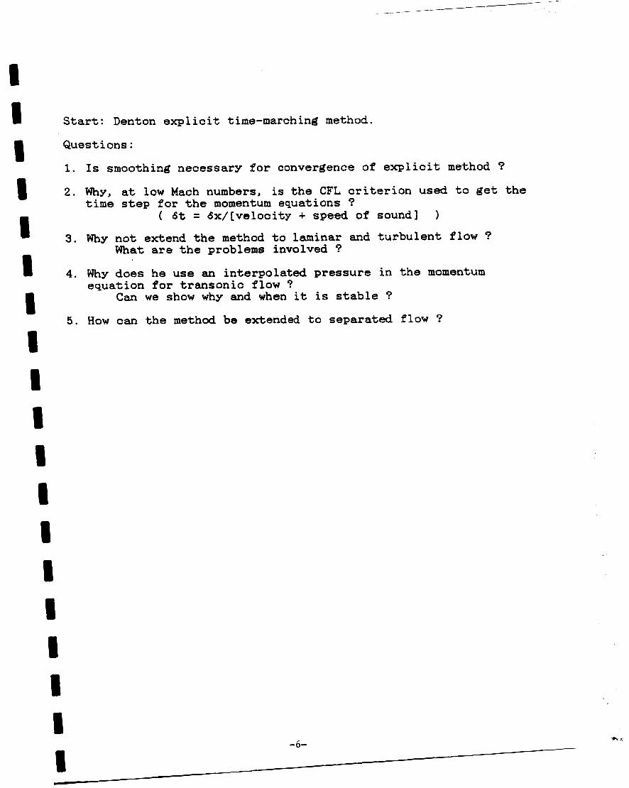
2. Why, at low Mach numbers, is the C F L criterion used to get the time step for the momentum equations ?

( 6t = Gx/[velocity + speed of sound] )

CONSERVATIVE FORM OF MOMENTUM EQUATION

u ap + v=pu 1 + Q ~ U + ~ U = V U = -ap + . . . at at ax

_. - -

continuity

- 6tcont - 6tmom included, therefore

Stability analysis, continuity and momentum

C F L condition b t = Sx/(u+c) CONVECTIVE FORM OF EQUATION

+ W * V U = -ap + , , , - - at b X

Stability analysis, momentum equation --- >

-9-

> ---

6t = 6x/u

I 1 I 1 I 1 I I I 1 I 1 I I I I I 1 I

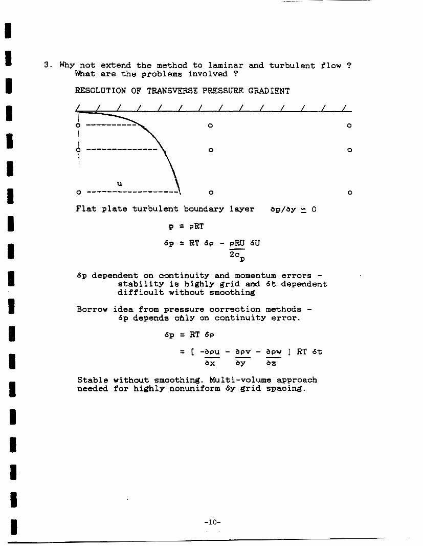
3. Why not extend the method to laminar and turbulent flow ? What are t h e problems involved ?

RESOLUTION OF TRANSVERSE PRESSURE GRADIENT

/ / / / / / / / / / / / / /

0 0

0 0

0

Flat plate turbulent boundary layer ap/ay 12 0

P = PRT 6p = RT Sp - pRU SU -

2cP

6p dependent on continuity and momentum errors - stability is highly grid and 6t dependent difficult without smoothing

Borrow idea from pressure correction methods - 6p depends ohly on continuity error.

Stable without smoothing. Multi-volume approach needed for highly nonuniform 6y grid spacing.

-10-

I 1 I I 1 I I I I I I I I 1 B I I 1 1

4. Why does Denton use an interpolated pressure in the momentum equation for transonic flow ?

Want apU + apv + apw = 0 ax 6Y az

Can we show why and when it is stable ?

- - - 1-D stability analysis. P = P + 6 0 u = u + 6 u

6u - c a(Sp>/aX 6p r RT ap

Interpolated pressure

+ Ai-l'pi-1 +. . . i+l Aidpi + = continuity error, each control volume

Exp 1 ic i t method approximation Il/stI &pi = continuity error for control volume

Stability requires Ai positive and dominant.

D I I I I I I I I D I I I I I I I I I

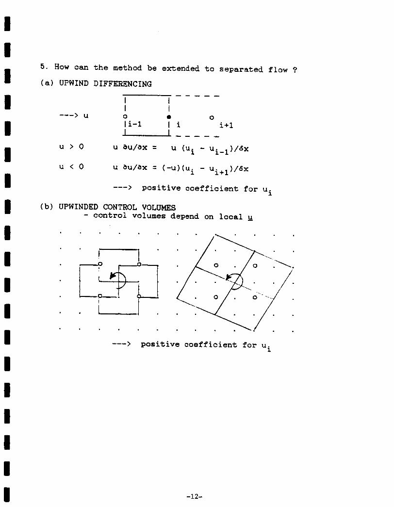
5. How can the method be extended to separated flow ?

(a) UPWIND DIFFERENCING - - - - -

I I I I 0 0 0 I i-1 t i i+l

> u ---

--- > positive coefficient f o r ui

(b) UPWINDED CONTROL VOLUMES - control volumes depend on local u

--- > positive coefficient for ui

-12-

I I I I I I I I I I I 1 I I I I I I I

3. LIST OF PROJECT REPORTS AND PAPERS

1. Nicholson, S . , "Development of a Finite Volume Time Marching Method," Turbomachinery Research Group Report No. JM/85-3, Mechanical Engineering Dept., VPI&SU, February 1985.

2. Nicholson, S., and Moore, J., "Semi-Annual Status Report on NASA Grant No. NAG 3-593 for the Period 12/20/84 - 5/31/85," Turbomachinery Research Group Report No. JM185-6, Mechanical Engineering Dept., VPI&SU, June 1985.

3. Moore, J., Nicholson, S., and Moore, J.G., "Annual Report on NASA Grant No. NAG 3-593 for the Period 12/20/84 - 12/19/85," Turbomachinery Research Group Report No. JM/85-11, Mechanical Engineering Dept., WICSU, December 1985.

4 . Nicholson, S., and Moore, J., "Semi-Annual Status Report on NASA Grant No. NAG 3-593 for the Period 12/20/85 - 5/31/86," Turbomachinery Research Group Report No. JM186-2, Mechanical Engineering Dept., VPI&SU, June 1986.

5. Nicholson, S., "Extension of the Finite Volume Method to Laminar and Turbulent Flow," Ph. D. Dissertation and Turbomachinery Research Group Report No. JM186-6, Mechanical Engineering Dept., VPI&SU, August 1986.

6. Nicholson, S., Moore, J.G., and Moore, J., "An Explicit Finite-Volume Time-Marching Procedure for Turbulent Flow Calculations," 5th International Conference on Numerical Methods in Laminar and Turbulent Flow, Montreal, Canada, July, 1987.

7. Nicholson, S . , Moore, J.G., and Moore, J., "Explicit Finite- Volume Time-Marching Calculations of Total Temperature Distributions in Turbulent Flow," 5th International Conference on Numerical Methods in Laminar and Turbulent Flow, Montreal, Canada, July, 1987.

-13-

I I I I I I I I I I I I I I I 1 I I I

4. BACKFLOW - EXTENSIONS TO THE COMPUTATIONAL PROCEDURE 4a. Discretization of Convection Terms

The momentum and energy equations are discretized over control volumes fixed relative to the grid points. Central differencing is used except in regions where there are large cross flows or backflow. In these regions a side upwind or reverse upwind differencing is used for’ stability. The details are as follows.

Control volume for momentum or energy for point i+l,j.

X X j+l

N

Bulk flow direction

> ----------

I I

w x I I

I I x E j I I

S

X

i X j-1

i+l

Convection of property I$ where cb = u for x-momentum

‘ I$ = v for y-momentum 4 = h for energy (enthalpy) equation.

Convection term integrated over control volume

We wish to express this in terms of the 0’s at the grid points, i. e we want the equation in the form

-14-


The coefficients C are determined from the mass fluxes through the sides (pgmA) and the discretization choice for 6NJ 4,., bEJ 6w, and

6,-

For stability we wish the center point coefficient, CEJ to be positive and greater than the sum of the other positive coefficients.

- @M - 'i, j take

to give a negative contribution to Cw.

take = @i+l, j

to give a positive contribution to CE.

@E and 4w

This centered evaluation of (second order accurate) gives a positive contribution to C E'

This upwind evaluation of 0, (first order accurate) gives a negative contribution to CEE.

This also determines aW since 4, for one control volume is @w for the next control volume.

-15-

I I 1 I I 1 I I I I I I I I I I I i I

The geometrical centered evaluation for 4, is

where F is the fraction of the distance of the North face between the grid points.

For accuracy this centered evaluation should be used whenever possible.

For stability when

When the inequality is chosen, which for equal grid spacing will occur when (SU-A)~ > Z(PU'A)E,

(the primary flow is locally backwards or zero relative to the bulk flow direction)

and

~

I I I 1 1 1 I I I I I 1 1 i 1 I I I I

When (pgU'A)N is negative, ( p u * A I , is positive for the next, the j+l, control volume, so that 6, is determined from 6, for the j+l control volume. Similarly when ( P U - A ) ~ is negative, +s is determined from 4N for the j-1 control volume.

ComDarison with earlier scheme.

In these terms, Nicholson (Section 3, Report 5 , JM/86-6) considered only positive values for ( P ~ = A ) ~ , i.e. no reverse flow. The formulae he used for +,, 6E and dW were the same as given here. However the upwinding he took for the cross flows was different. In particular when (pg-A) was positive, +, was evaluated using

N

Taking F 3 ( p ~ = A ) ~ / ( p u - A ) ~ gives lower and hence more conservative values of F when ( P ~ = A ) ~ > 2 ( p ~ * A ) ~ , i.e,, where for uniform grid spacing, the geometric F may not be used.

Present report / -

1 - I I

I

/ 0

I 0 /

N i cho 1 son * d - -

2 1 3 ,I 0 F I / d

r r d

- Geometric, :* uniform grid

0 0.5 1.0 (P~~A)E/(PU'A)N

high cross flow

low cross flow

F used in calculations.

-17-

0

0

t 2

5 a

m U G d 0 a

W 0

a 04 a &

a II

A U & a a 0 & a a p1 U 0

$

: 0 c)

L

I a 5 d

k 0 Er

m

r - - - - - I I

I

: /L - - - - a rl

4

-18-

0 0 V A

w z

w

m 0 II

W l Z

s

d l W

w l z A I

V 0

II

wlm

0 0

V A

w m

4b. Improved Pressure Interpolation for SBLI

The same Mach number dependent pressure interpolation formula for the calculation of the density used earlier is also used here. However to converge calculations with strong shock boundary layer interactions, i. e. with shock induced separations, the Mach number used in the formula needed to be changed from the local Mach number to the local free stream Mach number. Since stability is compromised if the Mach number is underestimated but not if it is overestimated, for simplicity, the value used was the largest Mach number on the relevant pair of i-surfaces.

X X

X I

I X

> ---- X I x

X I x

X X

X I

X

X

X

I

I X X X

X 'i+l I X

X I x X X X I

for these points Mmax

M = Mach number = maximum Mach number at planes i and i+l.

-19-

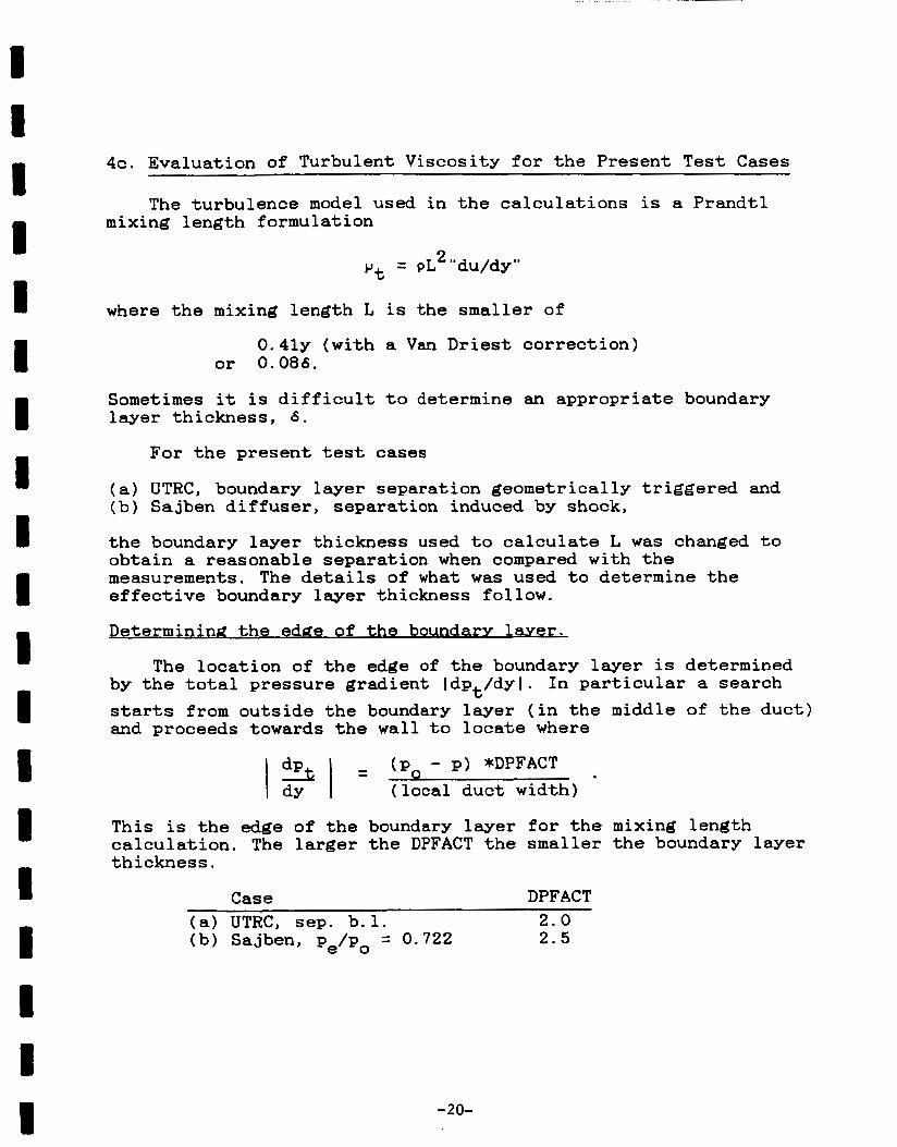
4c. Evaluation of Turbulent Viscosity for the Present Test Cases

The turbulence model used in the calculations is a Prandtl mixing length formulation

where the mixing length L is the smaller of

0 . 4 1 ~ (with a V a n Driest correction) or 0.086.

Sometimes it is difficult to determine an appropriate boundary layer thickness, 6.

For the present test cases

(a) UTRC, boundary layer separation geometrically triggered and (b) Sajben diffuser, separation induced by shock,

the boundary layer thickness used to calculate L was changed to obtain a reasonable separation when compared with the measurements. The details of what was used to determine the effective boundary layer thickness follow.

the edge of the bounda ry lauer. Determining . .

The location of the edge of the boundary layer is determined by the total pressure gradient Idpt/dyl. In particular a search starts from outside the boundary layer (in the middle of the duct) and proceeds towards the wall to locate where

- ( p - p) *DPFACT 1 % ) - I d Y I (local duct-width)

This is the edge of the boundary layer for the mixing length calculation. The larger the DPFACT the smaller the boundary layer thickness.

Case DPFACT (a) UTRC, sep. b. 1. 2.0 (b) Sajben, p,/po = 0.722 2.5

-20-

I I I I I I 1 1 D 1 1 I 1 I I I I i I

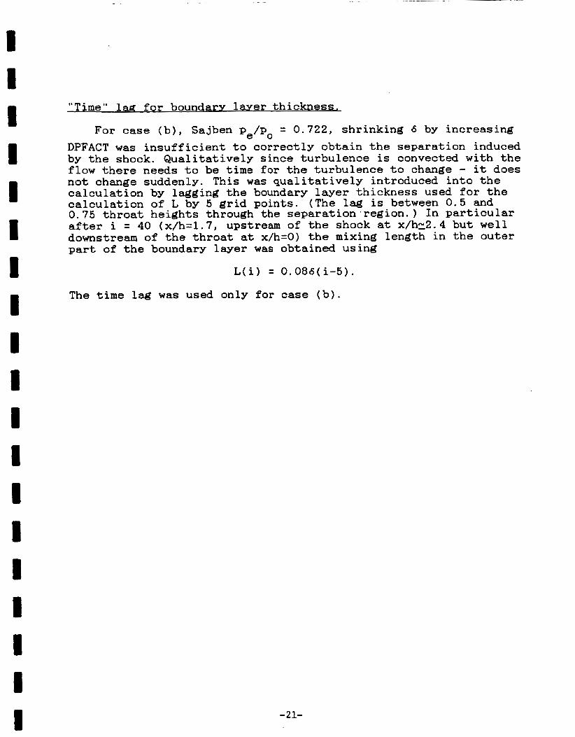
"Time" lag f o r boundary lay er thickness.

For case (b), Sajben pe/po = 0.722, shrinking 6 by increasing DPFACT was insufficient to correctly obtain the separation induced by the shock. Qualitatively since turbulence is convected with the flow there needs to be time for the turbulence to change - it does not change suddenly. This was qualitatively introduced into the calculation by lagging the boundary layer thickness used for the calculation of L by 5 gr id points. (The lag is between 0.5 and 0.75 throat heights through the separation.region.) In particular after i = 40 (x/h=1.7, upstream of the shock at x/hz2.4 but well downstream of the throat at x/h=O) the mixing length in the outer part of the boundary layer was obtained using

L ( i ) = O.O86(i-5).

The time lag was used only for case (b).

-21-

1 I 1 I

I 1 I I I I 1 I 1 I I I I I

m

5. BACKFLOW - TEST CASES The extensions to the computational procedure described in

section 4 were necessary for modelling two extreme cases of separated flow, the UTRC separated and reattached flat plate turbulent boundary layer (NASA Contract NAS3-22770, reference 1 ) and the MDRL transonic diffuser flow with a strong shock (MDRL Report N o . 81-07, reference 2 ) . These cases exhibit large boundary layer blockage (displacement thickness/local duct height), large backflow velocities, relative to the free stream velocity, and high rms/mean turbulence levels in the backflow region. The maximum boundary layer blockages were 58 percent (fifty eight!) in the UTRC low speed (Uref = 27 m/s) flow and 27 percent in the MDRL diffuser with a shock Mach number of 1 . 3 5 3 . The maximum backflow velocities were 37 percent and 25 percent, respectively, of the local maximum free-stream velocity. The ratios of rms/mean axial velocities at the locations of maximum reverse flow velocity were 35 percent in the UTRC flow and 66 percent in the MDRL diffuser. If the backflows in the two cases were varying sinusoidally, these values would correspond to maximum backflow velocities of - 5 . 4 2 2 . 7 m/s amd - 7 1 . 7 2 6 7 . 3 m/s, respectively.

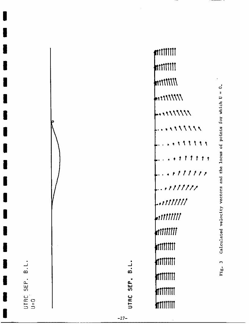
UTRC Separated and Reattached Turbulent Boundary Layer

The geometry and streamlines for flow through the UTRC test section are shown in Fig. 1; and laser doppler velocity measurements are shown in Fig. 2 . The corresponding calculated velocity vectors together with the locus of points for which U=O are seen in Fig. 3 . The size of the reverse flow region is well modelled, and the maximum calculated reverse flow velocity of - 4 . 1 m/s agrees well with the measured maximum value of - 5 . 4 m/s. This good agreement for the reverse flow leads to reasonable agreement between the measured and calculated values of skin friction coefficient in the separation zone, as shown in Fig. 4. The calculated locations of separation and reattachment are seen to be close to the measured locations. The good agreement in the separated flow region was obtained with the Prandtl mixing length model by reducing the turbulent viscosity in the boundary layer as discussed in section 4 (i.e. by using DPFACT = 2 . 0 ) . This then gave a corresponding decrease in the calculated skin friction upstream and downstream of the separation zone, as seen in Fig. 4 . We conclude that the present explicit computational procedure can be used for flows with extensive and strong backflow but that a more sophisticated turbulence model is required.

-22-


MDRL, Diffuser - Strong Shock Case

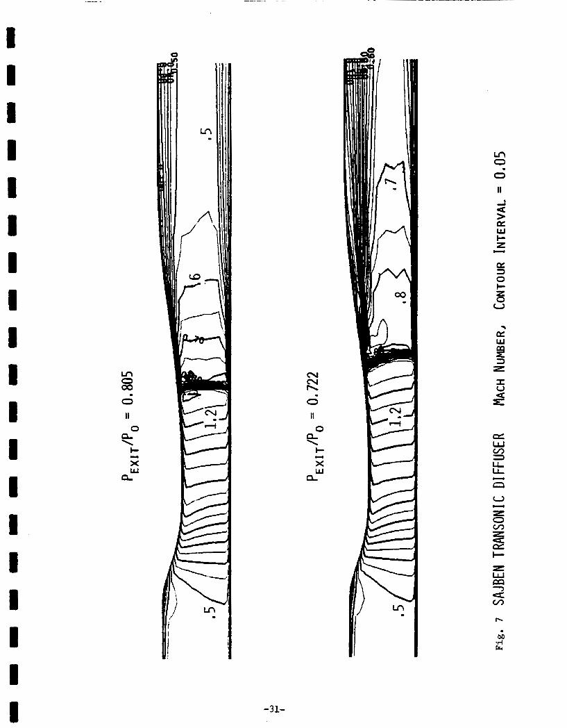
With a back pressure, pexit/po, inlet, of 0.722, the MDRL diffuser G had a shock Mach number of 1.353. Shock induced separation occurred in the turbulent boundary layer on the curved top wall. This contrasts with the case of 0.805 pressure ratio which gave a shock Mach number of 1.235 and no separation. In this section, results of calculations for these two flows will be compared, with particular attention being given to the backflow in the strong shock case.

The calculated shock locations are clearly seen for the two cases in the contours of static pressure in Fig. 5. The strong shock is located further downstream and shows evidence of a lambda foot at the curved top wall. The computed shocks are both quite sharp as a result of the use of the M&M pressure interpolation formula (see section 3 of this report, reference 3).

For the strong shock case, the computed and measured static pressure distributions on the top wall are compared in Fig. 6. The computed shock is just downstream of the measured lcoation and is therefore somewhat stronger with a shock Mach number of 1.39. Upstream of the shock the static pressures are indistinguishable; but downstream the calculated static pressures are consistently higher than those measured, perhaps partly because of three-dimensionality in the measured flow.

The Mach number contours in Fig. 7 show the flow accelerating up to the shock and decelerating downstream. The top wall boundary layer thickens appreciably more through the strong shock. This is seen also in the velocity vectors of Fig. 8, which show the separation bubble downstream of the strong shock. Fig. 9 shows this calculated backflow in more detail, and for comparison the magnitude and possible variations of the measured backflow are also shown. The maximum calculated backflow velocity of -87.7 m/s agrees quite well with the maximum measured value of -71.7 m/s.

Figures 8 and 9 demonstrate quite graphically the significant blockage caused by the separation bubble; and this is also seen in Fig. 10, which shows contours of total pressure.

We conclude that calculations of diffuser flows with strong shocks and shock induced separation can be performed with the present explicit method. As discussed in section 4, this calculation required a time lag of the turbulent viscosity to give a reduced viscosity in the separation bubble. In fact, this simple modification to the turbulence model produced a dramatic upstream movement of the shock and the calculation rapidly converged on a shock location close to that measured. Again this suggests the need for a more sophisticated turbulence model. But the present study of strong backflows has clearly demonstrated that they can

-23-

I 1 I I I I I 1 I I I I I I I I I I

i? 1

be modelled with an explicit method based on t h e f i n i t e volume approach.

References

1. P a t r i c k , W.P., "Flowfield Measurements i n a Separated and Reat tached F l a t P l a t e Turbulent Boundary Layer," NASA Cont rac t No. NAS3-22770, Draft F i n a l Report, August 1985.

2 . Salmon, J . T . , Bogar, T. J . , and Sajben, M. , "Laser Velocimeter Measurements i n Unsteady, Separated, Transonic D i f f u s e r Flows, " A I A A Paper No. 81-1197 (1981) . Accepted f o r p u b l i c a t i o n i n A I A A Jou rna l .

-24- . .

I I I I I I I I I I I I I I I I I 'I I

8 7

X

z- 0 I- d u 0 J c 2

A

L * =I c 0 C Q

E E c

-25-


-I

m

a W cn 0 ' u o !- II 3 3

e W m u a

-27-

t

0

0 e

CD 0

0

0

0 0

a

e

0

I " a 1 % l a ;

' B ' .a a I

I

I I I

- I I I I I I I I

O e I

0. I I I m

c .-

X

i 0 c C 0

-

9 -I

X 4 a

-28-

In 0 00 - 0 II 0 e \

I-

X w

M

n

E __---

F

cv N h

0

II

-

0 n \

I-

X - w e

-29-

cv 0

a > Q:

L

w Q: e 0

l-

I- v,

c(

a

CL

z 0 v,

CL I-

3

= w tp

v, 2

rn

M 94 r 4

.

i 1 I I I I I I I I 8 I I 1 I I I 1 1

c - / \ #

d -7-- -

Measured

Calculated _ e - - -

. 0

I I I I I I 1 I I I I I I I 1 - 5 - 4 - 3 - 2 - 1 0 1 2 3 II 5 6 7 8 9 10

A X I A L DISTANCE X / H

Fig. 6 Computed and measured static pressure distributions on the curved top wall of the MDRL diffuser. Strong shock case; p exi t'poinle t = 0.722.

-30-

0

0 II 0

e \ c

X W

I

e

0

0 II 0

e \ c X W

W e

In 0 I

0 II

I u r"

z w v) = LL L

I-

* M .rl F

-31-

1 I 1 I I I I I I I I I I I I I I I I

LA 0 00

0

0 II 0 e \

b w

X W e

hrtrrtrrl

cv cv h

0

0

0 e \ +

X W

U

e

-32-

v W > >- + U

u 0 J W > c1 W + 3 V J

u

4

a

p1 w v) e n L L U

u U

z 0

I-

I I

4 I I I I I I I I I I -33-

t m u 0 U

m \ E 0 0 U

0 0 e4

0

al rl P P 7 P

d U (d h a a al m al

9

9 c d

?I 3 a C (d

w 0

(d al h U m a 7 0 h 0 U L)

e

$ h U ?I U 0 rl

$ a al U a 4 3 L) rl (d U

o\

M .rl ra

.

I I

I

In 0 00 . 0 II 0 e \ c

X .L

W

I

Y c

-34-

cv cv h - 0 II 0 e \ t- X CI

W Q.

In cv 0

A > W t- z

a a

- a 3 0

9

0

t- e \

e 9

W

3 a

W

e a

A

t- 0

I-

a

w v, =I u, LL w n u - oz z e c z w m

0 rl

M d Frr


6. MACH NUMBER DEPENDENT INTERPOLATION FORMULA FOR DENSITY-UPDATE TIME-MARCHING METHODS

A 1-d stability analysis of density-pressure relations used in the computation of transonic flow was performed in Report No. JM/85-11 (see section 3 of this report, reference 3). Here we give a parallel development of a density interpolation equation for effective pressure for use in density-update methods. The formulae considered are tested using the density-update scheme outlined in Table 1.

Downwind Effective Pressure

In section 2.8 of reference 3, we considered an inconsistency in the pressure-density relation such that the pressure used in the momentum equation is offset by one grid point from the density used in the continuity equation, i.e.

In a density update method this may be viewed as an effective pressure evaluated downwind of its point of use in the momentum equations. This pressure-density relation was found to be stable for all Mach numbers, but it results in poor shock capturing as the calculated shock is spread over numerous grid points. Fig. 1 shows the calculated and theoretical pressure distributions for a 1-d calculation with a nominal shock number of 1.45.

Mach Number Dependent Interpolation Formula for Effective Pressure

In section 2.6 of reference 3, we saw that when the Mach number is high, the density update method is stable with the ideal gas equation of state satisfied at each grid point, i.e.,

(73)

Since this is the correct pressure-density relation for ideal gases it should be used where feasible. In this section, we will start with a generalized density interpolation equation for effective pressure

e. RTi with P i = P l

-35-

( 7 4 )

( 7 5 )

I I I 1 I I I I I I I I I D I I I I 1

and a 0 + a 1 + a 2 = 1

for second order accuracy.

We seek Mach number limitations to ao, al and a2 using the stability criterion that

the center point coefficient must be greater than the sum of the other positive coefficients,

‘Oefcenter > Sum Coef, .

Substituting

(46)

(77)

into Eq. 25 of reference 3 and rearranging in terms of the coefficients of each 6pi, a*, al, and a variations of A, u and c with i)

yields (neglecting 2’

1 al - 2 a2 1 2 3

( 2+MS(M+1) - 3ao

(-l-MS(M+l) + 3a + al + 2 a2 1 6 p i 3 0

( - a - 1 a1 - 1 a2 1 1 O 2 3

= h (781 change,i ‘

Now let us consider a simple second order scheme with a2 = 0 and a l = l - ao, and find limiting values of ao. From Eq. 74, it is obvious that we should consider only values in the range

-36-

I I I 1 B 1 I 8 1 I I I 1 I i I I I I

is positive or zero, and i+3 In this range, the coefficient of 6p

for the coefficient of 6pi+l (the center point) to be greater than the coeffcient of we require

a < 3 + 2 Mg(M+l). O 5 5

The coefficient of 6pi is positive when

- M3(M+1) > 0 or M(M+l) < Zao/3. 2a0

In this region, from Eq. 46, we require

or a < 1 + 4 Mg(M+l) . O 3 9

(83)

This criterion is more restrictive that Eq. 8 0 and the corresponding stability limit is shown as a function of Mach number in Fig. 2 for the conservative case of 3 = 1.0.

A set of equations for ao, a1 and a2, which satisfy the stability criteria (Eqs. 80 and 83) and give second order accurate interpolation (Eq. 7 6 ) has been selected; that is

a = 4 M(M+l) O 9

a1 = 1 - a.

az = 0.

This Mach number dependent formulation for a. and al is shown in Fig. 3. These equations are referred to as the M&M Mach number dependent interpolation formula for density-update time-marching methods.

-37-

Computational Tests of the M&M Density Interpolation Formula

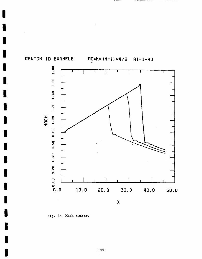
In this section, results of shock capturing with the M&M formula (Eq. 84) in the density update method (Table 1) are presented for Denton’s 1-d nozzle.

Calculation Details

Number of axial grid points = 46, 6x = 1 At inlet i = 1, M = 0.80 For air k = 1.4, R = 287. J/kgK ’exit”t, inlet = 0 . 8 5 , 0.80, 0 . 7 5

Results

The variations of static pressure, Mach number, and total pressure for all three back pressures are shown in Fig. 4. All three shocks are captured over four steps. The upstream side of the shock is sharply defined with only minor deviations from the theoretical 1-d solution. On the downstream side, there is a small overshoot and undershoot in static pressure and Mach number over two steps; the total pressure distributions show no overshoots or undershoots and show a sharp decrease over two steps.

Concluding Remarks

It is hoped that the M&M density interpolation formula will be useful to those organizations like NASA Lewis who are using density-update time-marching codes. It is also hoped that the stability analysis performed under this NASA Grant will be enlightening to users and developers of time-marching codes.

-38-

I Table 1.

I I 1 1 1 I I I I B R 1 1 1 i I i I

Outline of Effective Pressure Method with Different Time Steps - Density Update Scheme.

UNKNOWNS ( 2 - DIMENSIONS)

f s U s V s ( p u ) syv) s Po) ,ho,P,T

CONTINUITY

USING EQ. 2 - (U or V) TIMES EQ. 1

ENERGY

h - constant 0

-39-

B I

I I

OENTON 1D EXAMPLE RO= 0 A l = 0 0 0 Q)

0

0 0 OD

0

0 0 cc 0

0 0 CD

0

0 0 v)

.

.

.

=rd e 0 0 j l

0

0 0 rn 0

0 0 cu 0

0 0

0

0 0 0

0

.

.

. m

.

'J

0.0 10.0 20, 0 30.0 uo. 0 so, 0

X

Fig. 1 Comparison of calculated and theoretical 1-D static

pressure distributions, PW = '"t , inlet

theoretical ; calculated using a downwind effective pressure, Eq. 4

--

= 0.80. 'exit" t , inlet Grid spacing, 6x = 1;

-40-

I I I I I I I I I 1 1 I I I I I I I I

a

8 ni

3 0

d

0 '9

0 1: CI

0

9 4

0

0 x 0 (Y

0

8 0

STRBILITY LIMITS, RO+FIl=l

0.00 0.20 0.W 0.10 0.60 1.00 1.20 I.YO 1.60 1.60 2-00 2.20 2.W 2.60 2.80 3.00

MRCH

Fig. 2 M C M density interpolation formula for use with

Effective Pressure, Density Update, T i m e Marching Methods.

Stabi l i ty limits for a. when a2 - 0 and a. + al = 1.

-41-

I I I I I I 1 I I I I I I I I I I 1 I

0 x 0 m L

0 '4 - ? c.

0 N LI

0 9

%

a c.

0

@! 0

0

d

N. 0

0

5 0

1

I I I 1 , I I I a

0.00 Q.ZO 0.PO 0.80 0.80 1.00 1.20 I .YO 1-80 1.80 2.00 2.20 2 e Y O 2-80 2-W 3 . 0 0

MRCH

Fig. 3 M & M Mach number dependent values for the density interpolation

coef f ic ients , a. and a i n the Effective Pressure Method. 1'

-42-

I I I I I I I I I I I I I I I I I I - I

DENTON 1D EXFlMPLE RO=Hn ( M + J ) 4 / 9 Al=l-RO

PW =

0 0 m 0

0 0 aD 0

0 0 l-

0

0 0 W

0

0 0 v,

.

.

= & e 0 0 3

0 . 0 0

'"t , i n l e t c3 . 0

0 0 cu 0

0 0 - 0

0 0 0

0

W

0.0 10.0 20.0 30.0 go. 0 50 .0

X

Fig . 4a Calculated 1-D solution for Denton's nozzle

using M & M density interpolation formula

with the Nicholson/Moore Effect ive Pressure,

Density Update Method.

Calculations for three e x i t s t a t i c pressures a t x = 4 6 . ,

'exi t'pt, in l e t = 0.85, 0.80, and 0.75.

-43-

I I I

L - - -

DENTON 1D EXRMPLE

0 Q3 . CI

0 io . -.

0 N . d

0 W

0 . 0 s 0 . 0 Iu

0 .

0 0

0 . 0.

I 1 I I I I I I I

L 1

1 L I

I t I 1

0 10.0 2 0 . 0 30.0

X

uo. 0 50.0

Fig. 4b Mach number.

-44-


- I I I I I I I 1 I 1

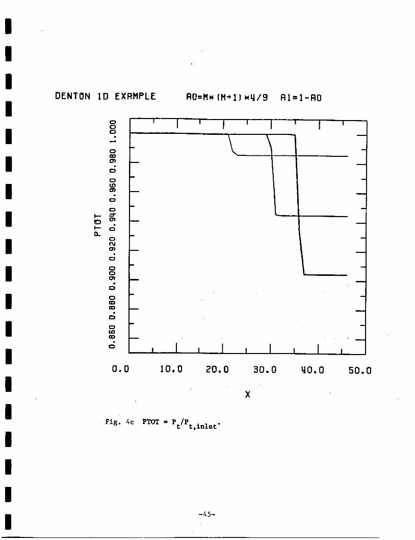
DENTON 10 EXAMPLE AO=M* [ M + 1 1 nU/9 Al=l-RO

0

0

0

g z + d L

0 N m 0

0 0 Q)

0

.

. 0 OD OD

8

0

. 0

E 1

0 . 0 10.0 20.0 30.0

X

Fig. 4c PTOT = Pt/Pt,inleto

-45-

‘40.0 50.0

I I I I I I D I I I I I I I I I I I I

APPENDIX A

TITLE PAGES AND ABSTRACTS OF REPORTS

prepared in connection with

NASA GRANT NO. NAG 3-593

-46-

4

4

Development of a F in i t e Volume

Time Marching Method

bY Stephen Nicholson

February 1985

4

Turbomachinery Research Group

Report No. Jn/85-3,

Mechanical Engineering Department

Virginia Polytechnic Ins t i tu te and State University


-47-

DEVELOPKENT OF A FINITE VOLUME TIME MARCHING METHOD

ABSTRACT

The objective of the current work is to develop and demonstrate a

Navier-Stokes approach for transonic flow which includes viscous

terms in the finite-volume method. The accuracy of the

computational method will be verified using a transonic diffuser

as a test case. The computational goal is to calculate the flow

in sufficient detail and with sufficient accuracy that the loss

generating mechanisms can be studied to assess the sources of

inefficiency in the transonic diffuser. The purpose of this

report is to document progress made in the development of the

time-marching finite-volume method from September 1984 to Decewber

1984.

Semi-Annual S t a t u s Report on

NASA Grant No. NAG 3-593

Thermodynamic Evaluation of Transonic Compressor Rotors Using the F i n i t e Volume Approach

for t he per iod 12/20/84 - 5/31/85

by Stephen Nicholson

Ins t ruc to r and


Pr inc ipa l Inves t iga to r

Grantee I n s t i t u t i o n - NASA Lewis Research Center



Report No. JM/85-6


Vi rg in ia Polytechnic I n s t i t u t e and S t a t e Universi ty Blacksburp, Vi rg in ia 24061

-49-

EXTENSION OF A F I N I T E VOLUME EXPLICIT TIME MARCHING METHOD TO

LAMINAR AND TURBULENT FLOW

ABSTRACT

This r epor t documents progress made i n extending t h e f i n i t e

volume e x p l i c i t time marching method t o laminar and t u r b u l e n t

flow during the t i m e per iod from January t o May 1985. The work

done is under NASA g r a n t NAG 3-593. Previously, ex tens ions had

been made t o t h e f i n i t e volume method t o improve t h e accuracy of

t h e c a l c u l a t i o n of t o t a l p ressure i n compressible i n v i s c i d flow.

These changes a r e documented i n re fe rence 1 . The c u r r e n t work

extends these ideas and develops new ideas which allow t h e

c a l c u l a t i o n of laminar and tu rbu len t boundary l a y e r s i n i n t e r n a l

flows. The method is v e r i f i e d using fou r t e s t cases wi th

free-stream Mach numbers ranging from .075 t o 1.20.

-5c-

I I I I 1 I I 1 I I 1 I

Grantee I n s t i t u t i o n - NASA L e w i s Research Center


Annual Report on NASA Grant No. NAG 3-593

Thermodynamic Evaluat ion of Transonic Compressor Rotors Using the F i n i t e Volume Approach

f o r the per iod 12/20/84 - 12/19/85

by John Moore

P ro fes so r of Mechanical Engineering P r i n c i p a l I n v e s t i g a t o r

Stephen Nicholson I n s t r u c t o r

and Joan G. Moore

Research Assoc ia te


Report No. JM/85-11


V i rg in i a Poly technic I n s t i t u t e and S t a t e Un ive r s i ty

Blacksburg, V i rg in i a 24061

-51-

Abs tract

Summer research a t NASA Lewis Research Center gave the oppor tun i ty to inco rpora t e new c o n t r o l volumes i n the Denton 3-D finite-volume time- marching code. For duc t flows, the new c o n t r o l volumes require no t r ansve r se moo th ing and th i s allows c a l c u l a t i o n s with l a r g e t r ansve r se g r a d i e n t s i n p r o p e r t i e s without s i g n i f i c a n t numerical t o t a l p re s su re lo s ses .

The summer research a l s o pointed t o p o s s i b i l i t i e s f o r improving the Deuton code to o b t a i n b e t t e r d i s t r i b u t i o n s of p r o p e r t i e s through shocks. Much better t o t a l p ressure d i s t r i b u t i o a s through shocks are obtained when the i n t e r p o l a t e d e f f e c t i v e pressure, needed to s t a b i l i z e t h e s o l u t i o n procedure, is used t o calculate the t o t a l pressure. This s imple change l a r g e l y e l imina te s the undershoot i n t o t a l pressure down- s t ream of a shock. Overshoots and undershoots in t o t a l p re s su re can then be f u r t h e r reduced b9 a f a c t o r of 10 by adopt ing the e f f e c t i v e d e n s i t y method, developed a t VPIdSU, rather than the e f f e c t i v e pressure method. Use of a Mach number dependent i n t e r p o l a t i o n scheme f o r pres- s u r e then removes the overshoot i n s tatic pressure downstream of a shock.

The s t a b i l i t y of i n t e r p o l a t i o n schemes used f o r the c a l c u l a t i o n of e f f e c t i v e dens i ty is analyzed and a Mach number dependent scheme, the M&M formula, is developed. This formula combines the advantages of the c o r r e c t p e r f e c t gas equa t ioa for subsonic flow wi th the s t a b i l i t y of 2- p o i n t and 3-point i n t e r p o l a t i o n schemes f o r supersonic flow.

I I 1 I I I I I I I 1 I I I 1 I I I I -52-

I I I I I I I I I 1 I I I I I I I I

Semi-Annual Status Report on


Thermodynamic Evaluation of Transonic Compressor Rotors Using the Finite Volume Approach

for the period 12/20/85 - 5/31/86

by Stephen Nicholson

Instructor and


Principal Investigator

Grantee Institution - NASA Lewis Research Center



Report No. JM/86-2


Virginia Polytechnic Institute and State University Blacksburp, Virginia 24061

-53-

I I I I I I I I I I I I I 1 I I I I I

ABSTRACT

This report documents progrcss made is refining and improving the finite-volume explicit time

marching method (1, 2, and 3 ) during the t h e pexiod from January to May 1986. The work is

done under NASA grant NAG 3-593. Pnviously, extension had betn made to the finite volume

method to

1. improve the accuracy of the calculation of total pressure in inviscid flow (1).

2. extend the method to allow the calculation of laminar and turbulent boundary layers in internal

flows (2).

3. improve the shock capturing properties of the method by introducing a Mach number de-

pendent interpolation scheme for the pressure used in the calculating the density (3).

The ament work exten& these developments by

1. using the new pressure interpolation scheme in two dimensional viscous calculations.

2. including a more complete desaiption of the viscous stresses.

3. introducing a criteria for the transvtrse upwind diffenncing which is a kction of the ratio of

transvast and streamwise mass fluxes.

4. dowing the calculation of %tend flow where boundary layers are present on both wall of the

duct.

Specifically, this nport is broken up into three sections. Section 1 discusses in detail the mauner

in which the viscous stresses arc evaluated in the non-orthogonal, non-uniform grid. Section 2 in-

vestigates the convergence and presents results for calculations of laminar flow in a converging duct.

-54-

I I I I I 1 I I I I I I I I I I I I I

Section 3 presents results for calculations of transonic turbulent flow in a converging-diverging

nozzle; the results are compared with Sajben's measurements and calculations by other authors.

-55-

7- ,g ir! ,’

I I I I I I I I I I I I I I I I

I I

Turbomachinery Research Group I Report No. JM186-6


V i r g i n i a Po ly techn ic I n s t i t u t e and S t a t e Un ive r s i ty

Blacksburg, V i r g i n i a 24061

-56-

S t a t u s Report - August 1986 on


Thermodynamic Evalua t ion of Transonic Compressor Rotors Using t h e F i n i t e Volume Approach ---

Extension of t h e F i n i t e Volume Method t o Laminar and Turbulent Flow

bY Stephen Nicholson

I n s t r u c t o r

John Moore P r o f e s s o r of Mechanical Engineer ing

P r i n c i p a l I n v e s t i g a t o r

---

Grantee I n s t i t u t i o n - NASA Lewis Research Center


I I 1 I I 1 I i R i I I I B D 1 I I I

Extension of the Finite Volume Method

to Laminar and Turbulent Flow

bY

Stephen Nicholson

John Moon, chairman

Mechanical Engineering

(ABSTRACT)

A method has been developed which calculates two-dimensional, transonic, viscous flow in ducts.

The finite volume, time marching formulation is used to obtain steady flow solutions of the

Reynolds-averaged form of the Navicr Stokes quations. The mtirc calculation is performed in the

physical domain. The method is currently limited to the calculation of attached flows.

The fa- of the current method can be summanztd as follows. Control volumes are chosen so

that smoothing of flow properties, typically required for stability, is not needed. Different time steps

arc used in the differcnt governing quations to improve the convergence speed of the viscous cal-

culations. A new pressun interpolation scheme is introduced which impmvcs the shock capturing

ability of the method. A multi-volume method for pressure changes in the boundary layer allows

calculations which use very long and thin control volumes ( rCngth/height S 1000). A special

discretization technique is also used to stabilize thew calculations which use long and thin control

volumes. A special formulation of the energy quation is used to provide improved transient be-

havior of solutions which use the full en- quation.

\

The method is then compand With a wide varkty of test cases. The frttstrcam Mach numbers

range from 0.075 to 2 8 in the calculations. Trarwonic viscous flow in a converging diverging nozzle

is calculated with the method; the Mach number upstream of the shock is approximately 1.25. The

agreement between the calculated and measurcd shock strmgth and total pressure losses is good.

Essentially incompressible turbulent boundary layer flow in an adverse pressure gradient is calcu-

lated and the computed distribution of mean velocity and shear stress are in good agreement with

-57-

the measurements. At the other end of the Mach number range, a flat plate turbulent boundary

layer with a &stream Mach number of 2.8 is calculated using the full enerpy equation; the com-

puted total temperature distribution and recovery factor agree well with the measurements when a

variable Prandtl number is used through the boundary layer.

-58-

I

APPENDIX B

An E x p l i c i t Finite-Volume Tine-Harching Procedure for Turbulent Flow Q l c u l a t i o n s

Stephen Nicholson, Joan G. Moore and John Moore

Mechanical Engineering Department V i rg in i a Polytechnic I n s t i t u t e and S t a t e Universi ty


1. SUMMARY

A method has been developed which calculates two- dimensional, t ransonic , viscous flow i n ducts . The f i n i t e - volume, time-marching formulation is used t o ob ta in steady flow so lu t ions of the Reynolds-averaged form of the Navier Stokes equat ions. The e n t i r e c a l c u l a t i o n is performed in the phys ica l domain.

The f e a t u r e s of t h e cur ren t method can be summarized as follows. Control volumes a re chosen so t h a t smoothing of flow p rope r t i e s , t y p i c a l l y required f o r s t a b i l i t y , is no t needed. D i f f e ren t time steps are used i n the d i f f e r e n t governing equations. A new pressure i n t e r p o l a t i o n scheme is introduced which improves the shock captur ing a b i l i t y of the method. A multi-volume method f o r pressure changes in the boundary l a y e r a l lows ca l cu la t ions which use very long' and t h i n c o n t r o l volumes ( lengt ldhe ight - 1000). The method i s then compared here with two test cases. E s s e n t i a l l y incom- p r e s s i b l e tu rbu len t boundary l aye r flow i n a n adverse pressure g rad ien t is ca lcu la t ed and the computed d i s t r i b u t i o n s of mean v e l o c i t y and shear stress a r e i n good agreement wi th the measurements. Transonic viscous flow in a converging diverging nozzle is ca lcu la t ed ; the Mach number upstream of t h e shock is approximately 1.25. The agreement between the c a l c u l a t e d and measured shock s t r e n g t h and to t a l pressure l o s s e s is good.

2 . INTRODUCTION

The f i n i t e volume method has been used ex tens ive ly to so lve the E u l e r equat ions €or t ransonic flow including flow a t high i%ch numbers. In i n t e r n a l aerodynamics, McDonald [ l ] was the f i r s t i n v e s t i g a t o r t o use the time marching f i n i t e volume method. Denton [2 ] extended YcDonald' s f i n i te-volume

-5 9-

1 I 1 I I 1 D 1 1 1 1 I 1 I I i 1 I I

method to three dimensions. Versions of Denton's method have been used in inviscid-viscous i n t e r a c t i o n programs f o r turbomachinery c a l c u l a t i o n s [ 3-51 .

The scope of the present work was t o extend a f i n i t e volume method l i k e t h a t o€ Denton's t o be a b l e to calculate laminar o r t u rbu len t flow in ducts. The new method has the c a p a b i l i t y t o c a l c u l a t e subsonic as w e l l a s t r anson ic flow.

3. GOVERNING EQUATIONS

The unsteady form of the con t inu i ty equat ion, the x'

momentum equat ion , and the y-momentum equat ion, i n i n t e g r a l form, are used to ob ta in a s teady-s ta te s o l u t i o n f o r flow through 2-dimensional ducts. The i d e a l gas equat ion of s ta te , the assumption of constant t o t a l temperature, and a P rand t l mixing length turbulence model complete the governing equat ions needed to so lve f o r t he unknown v a r i a b l e s p , u , v, P, v , and T.

For a f i n i t e c o n t r o l volume where we can va lue of dens i ty to the control volume, and f o r a s t e p , 6 t , c o n t i n u i t y states that,

6 t - P" = 6P = -[JJ p u - %I pn+l

where the i n t e g r a l is evaluated e x p l i c i t l y a t time s t e p , n. In a r r i v i n g a t an express ion which

assign one f i n i t e time

the c u r r e n t relates the

pressure change d i r e c t l y t o the con t inu i ty e r r o r , w e w i l l assume that changes i n temperature a r e ma11 i n comparison to o t h e r changes f o r one time step. Thus, w e can relate changes i n pressure t o changes in densi ty through the i d e a l gas equat ion of state,

For the method introduced i n the c u r r e n t work, a non-conser- v a t i v e form of the unsteady momentum equat ion is used. The non-conservative form is used because it al lows the u s e of d i f f e r e n t t i m e s teps f o r t h e con t inu i ty and momentum equa- t i ons . The d i f f e rences be tween the non-conserva t i v e and conserva t i v e f oms of the unsteady momen tum equat ions a r e a s s o c i a t e d with the unsteady and convective terms . S p e c i - f i c a l l y , w e no te t h a t

a ( P U > a u

-60-

I 1

and the r i g h t hand s i d e of Eq. (3) can be r e w r i t t e n as

a U au (4)

- - + v pu u - u(V pu) P a t + p u . v u = p = - - - - When the r i g h t hand s i d e of Eq. (4) i s combined with the pressure and viscous terms, the momentum equat ion i n i n t e g r a l form becomes

-

To maintain s t a b i l i t y , the p rope r t i e s mus t be updated in t he proper sequence. In the current method, t he sequence is 1. update the pressure from the c o n t i n u i t y equat ion; 2. update the v e l o c i t i e s from the momentum equat ion using

the new p res su re and o l d v e l o c i t i e s and o l d dens i ty ; 3. update the dens i ty from the i d e a l gas equat ion of s ta te ; 4. update the temperature from cons tan t t o t a l temperature.

4. CONTROL VOLUMES

A new c o n t r o l volume has been introduced f o r t h i s method. To e l imina te the need f o r smoothing of flow proper- t ies, t h e r e must be as many con t ro l volumes a c r o s s the duct as t he re are nodes where these v a r i a b l e s are ca l cu la t ed . We need as many equat ions as unknowns. The c o n t r o l volumes a l s o need t o be located so t h a t e r r o r s in c o n t i n u i t y and momentum can c o r r e c t l y in f luence the changes in pres su re o r dens i ty and v e l o c i t y without smoothing. The c u r r e n t c o n t r o l volume accomplishes t h i s and is shown in Fig. 1. When c a l c u l a t i n g the f l u x through a streamwise f a c e of an element, the value of the flow p r o p e r t i e s a t the node on that f a c e are used. Linear i n t e r p o l a t i o n is used to o b t a i n the f l u x on the cross- stream face.

GRID POINC

Fig . 1 New Control Volumes I

-61-

1 I I I I 0 I I I I I I I I 1 I I I I

5 . DISTRIBUTION OF PROPERTIES

The p rope r t i e s a t node points are changed i n the flow f i e l d a f t e r each t i m e step because the con t inu i ty and momentum equat ions are no t s a t i s f i e d f o r a given c o n t r o l volume. A decis ion must be made about which node, e i t h e r upstream o r downstream, these changes should be a l l o c a t e d to. The c r i t e r i o n used in determining where changes i n p r o p e r t i e s should be s e n t is t h a t these d i s t r i b u t i o n s resu l t i n reduced e r r o r s i n cont inui ty and momentum. The c u r r e n t method uses the following a l l o c a t i o n procedure: 1. The pressure is updated through the con t inu i ty equat ion

and t h e pressure change is s e n t t o the upstream node; 2. The u and v v e l o c i t i e s are updated through the momentum

equat ions and the changes are s e n t to the downstream node;

3. The dens i ty is updated through the i d e a l gas equat ion of state using an in te rpola ted pressure.

6 . PRESSURE INTERPOLATION PROCEDURE

As p a r t of the updating procedure used by Denton [ 5 ] , an e f f e c t i v e pressure is used i n the momentum equat ions r a t h e r than the t rue thermodynamic pressure determined from the i d e a l gas equat ion of s t a t e . This e f f e c t i v e pressure is needed because i f the t r u e pressure is used i n the momentum equat ions the so lu t ion m y n o t converge. I n the c u r r e n t method, the dens i ty used i n t h e con t inu i ty and momentum equat ions is an e f f e c t i v e densi ty which may be d i f f e r e n t than the dens i ty obtained using t h e i d e a l gas equat ion of state. This e f f e c t i v e dens i ty is used requirements.

S t a r t i n g with a general ized equat ion €o r the e f f e c t i v e density

t o s a t i s f y s t a b i l i t y

pressure i n t e r p o l a t i o n

(pI+l - pH) al 2 +

Mach number l i m i t a t i o n s were sought f o r ao, al, and a2 such t h a t

a l + a2 + a3 = 1 (7)

which assures second order accura te so lu t ions . A set of equat ions f o r ao, a l , and a 2 was chosen which sat isf ies two s t a b i l i t y cri teria [ 6 ] . The equations are

-6 2-

1 I 1 I I I I I I I I I I 1 I I I 1 r

f o r M G 2 0.8 4 M

a. = (T) (7 -1) ; al = 1 - ag ; a2 = o :

f o r M > 2 ag = 0 ; al = 4/M2 ; a2 = 1 - al . ( 8 )

These Mach number dependent formulations f o r ao, a19 and a2 are shown i n Fig. 2.

0 1 2 3 I.lACH NlMBER

Fig. 2 Mach Number Dependent Values f o r Coeff ic ients ag , al, and a2

7. TIME STEPS

A unique f e a t u r e of t h i s method is the use of d i f f e r e n t time s t e p s f o r the cont inui ty and momentum equations. Previous workers who have used e x p l i c i t t i m e marching methods have used the CF'L condition as a b a s i s for determining a l lowable t i m e s t e p s which maintain s t a b i l i t y . The same time s t e p is used f o r both the c o n t i n u i t y and momentum equations. In the c u r r e n t method, t he express ions t h a t are used t o determine the allowable time s teps are; f o r t he momentum equat ions

6 t m 1

and f o r c o n t i n u i t y ,

where 6tm i s the momentum time s t e p , 6 t c 1s the c o n t i n u i t y time s t e p and veff fs an e f f e c t i v e y-component of ve loc i ty . The advantage of using d i f f e r e n t time s teps is t h a t , for low

-63-

I I I

I I I I I

I 1 I 1

v e l o c i t y regions of the flow, the al lowable momentum time s t e p can be s i g n i f i c a n t l y larger than t h a t allowed by the CFL condition. These l a r g e r time steps allow the boundary l a y e r p r o f i l e s to change more rapidly and enhance the convergence ra te s i g n i f i c a n t l y compared with a method which uses the CFL condi t ion.

8. BOUNDARY CONDITIONS

For viscous flow, a t the upstream boundary, t h e t o t a l temperature, f r e e s tream t o t a l p ressure , i n l e t boundary l a y e r v e l o c i t y p r o f i l e , and flow angle are Specif ied. Along the downstream. boundary the s t a t i c pressure is spec i f i ed . Pres- sures along the s o l i d boundaries are determined from l i n e a r ex t r apo la t ion . For viscous flow, the va lues of the x- component and y-component of v e l o c i t y are set equa l to zero a t s o l i d walls.

9 . TURBULENCE MODEL

A Prandt l mixing length model is used t o model t h e t u rbu len t stresses. The model is

31 pL2 "du" v t 3

L is smaller of 0.08 times the width of boundary l a y e r o r 0.41 times the d i s t ance t o the wall

Van Driest Correct ion

L = 0.41 " ~ " ( 1 - em[- "y" J c / 2 6 p e l >

Gear wall Correct ion

10. MULTI-VOLUME METHOD FOR PRESSURE CHANGES

Control volumes are grouped in t he boundary l aye r t o form a l a r g e r g loba l con t ro l volume. The con t inu i ty e r r o r is c a l c u l a t e d f o r t h i s g loba l con t ro l volume and changes in pres su re are assigned equal ly t o each of the upstream nodes f o r each c o n t r o l volume making up the g loba l con t ro l volume. Then the g loba l cont ro l volume is made success ive ly smaller towards the wall. This is shown schematical ly in Fig. 3. The e n t i r e pressure change f o r one i t e r a t i o n a t each node wi th in the multi-volume region is determined by adding toge ther a l l the pressure changes assigned t o t h a t node.

The multi-volume method propagates pressure changes r a p i d l y through the boundary l aye r and minimizes t ransverse p re s su re g rad ien t s i n the intermediate so lu t ion . The above changes al low the ca l cu la t ion of boundary l a y e r flows where

-64-

I I I I I I I I I I ‘I I I I I I I I I

t h e c o n t r o l volumes near the wall can have a s p e c t r a t i o s ( l eng th /he igh t ) over 1000.

VOL. 1 VOL. 2 VOL. 3 VOL. 4

Fig. 3 Multi-Volume Method f o r Pressure Changes i n t h e Boucdary Layer

11. TRANSVERSE UPWIND DIFFERENCING

When the con t ro l volumes become long and th in near the wall of t he duct , the f luxes through the top and bottom faces of the c o n t r o l volume become more s i g n i f i c a n t i n comparison t o the f l u x e s through the streamwise faces . To s t rengthen the diagonal dominance of t he c o e f f i c i e n t matrix, the momentum f luxes through the t ransverse faces m y be calcu- l a t e d using in t e rpo la t ed v e l o c i t i e s upstream i n the t r ansve r se d i r e c t i o n r a t h e r than the actual in t e rpo la t ed values. The i n t e r p o l a t i o n funct ions and the de r iva t ion of t h e func t ions is discussed in more d e t a i l in Ref. 6.

12. SAMUEL AND JOIJBERT INCOMPRESSIBLE TURBULENT BOUNDARY LAYER

Incompressible turbulent boundary l a y e r flow in a d iverg ing duc t was c a l c u l a t e d for test case 0141 of the S tanford Conference [ 7 ] . The g r i d used in t he p re sen t c a l c u l a t i o n s is shown i n Fig. 4. The i n l e t ve loc i ty is 26 m/s .

Fig. 4 Geometry and Grid f o r Samuel and Joubert

Figure Sa shows a comparison of the ca l cu la t ed sk in f r i c t i o n c o e f f i c i e n t with the experimental results and with the results from the iloore cascade flow program. The agreement is exce l l en t . A comparison of the calculated t u r b u l e n t shear stress d i s t r ibu t ion , z, w i t h the experi-

-65-

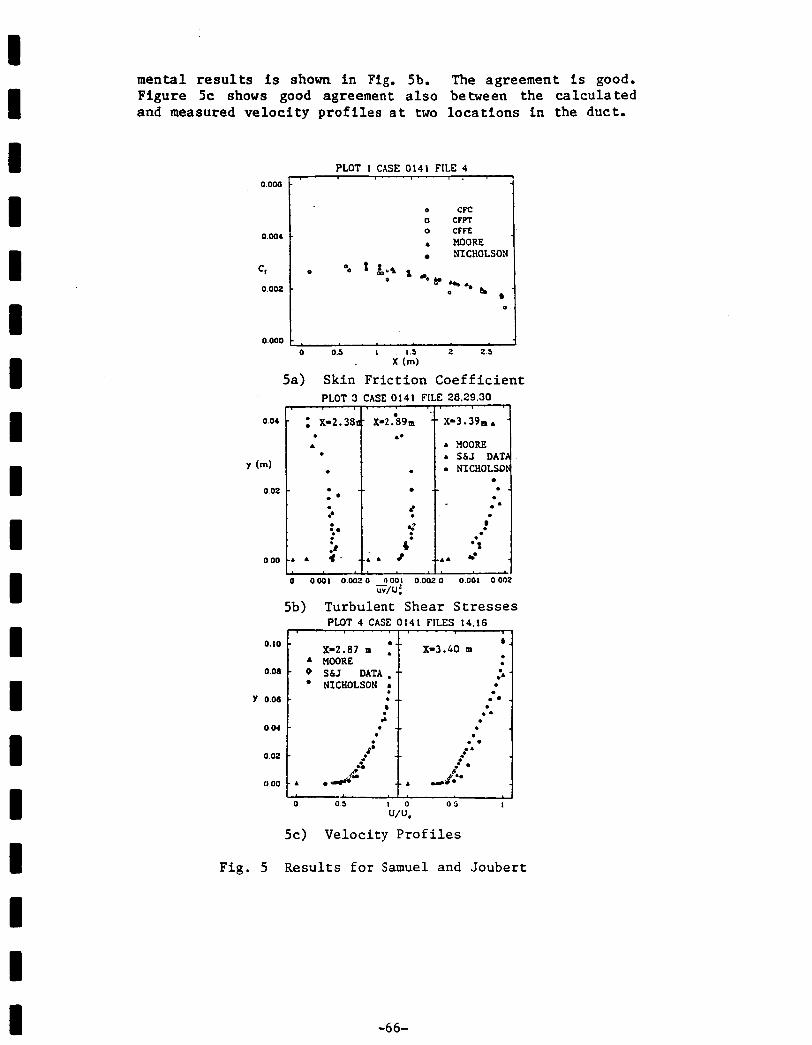
mental resul ts is shown i n Fig. 5b. The agreement is good. Figure 5c shows good agreement a l so between the calculated and measured ve loc i ty profi les a t two locations i n the duct.

PLOT 1 CASE 0141 FILE 4 0.ow F 4

0.004 I - 0 CFC 0 CFPT 0 CFW

NICHOLSON A MOORE

0.000 , J 0 0.5 I 1.5 2 2.5

X (m)

5a) Skin Friction Coefficient PLOT 3 CASE 0141

0

A . Y (m) .

0.02 - . . * c :* .#

. . . 000 -A A 4 '

o 0.001 0 . 0 0 ~ o -noo! 0002 o 0.001 o on2 uv/u;

5b) Turbulent Shear Stresses PLOT 4 CASE 0141 FILES 14.16

0.10

0.08

Y 0.08

0.04 : t

8 X-3.40 m .

.A

0 . . . .. . . .

0 0 5 I O 0 4 I wu.

5c) Velocity Prof i les

Fig. 5 Results for Samuel and Joubert

-66-

13. MDRL DIFFUSER CALCULATIONS

The d i f f u s e r geometry (Model G) is shown i n Figure 6a [ 8 , 9 ] . Figure 6a a l s o shows the computational g r i d used which has 87 g r i d p o i n t s i n t h e a x i a l d i r e c t i o n and 20 p o i n t s a c r o s s the flow. The i n l e t boundary l a y e r thicknesses were s p e c i f i e d as 9% and 4.5% of t h e i n l e t d i f f u s e r h e i g h t f o r the curved and f l a t wall boundary l a y e r s , r e spec t ive ly . For t h i s c a l c u l a t i o n , t he r a t i o of e x i t s ta t ic p res su re t o the i n l e t t o t a l p ressure was 0.826. In the experiment, t h i s t e s t p o i n t r e s u l t s i n t r anson ic flow in t he diverging por t ion of t h e duc t with a Mach number of approximately 1.235 upstream of a n e a r l y normal shock, and the flow remained fully-a t tached throughout the d i f f u s e r a t th i s test condition.

A contour p l o t of s t a t i c pressure is shown i n Fig. 6b. The shock can be seen i n the diverging po r t ion of the duct. The shock is w e l l def ined as i l l u s t r a t e d by the high c l u s t e r i n g of contours a t the shock. Figure 6c shows a Flach number contour p l o t f o r the calculat ions. The c a l c u l a t e d and measured curved wall s t a t i c pressures are compared i n Fig. 7. The shock is w e l l defined and no overshoot occurs €n the s ta t ic pressure. rx

a) geometry and g r i d

b) s ta t ic pressure contours

c) Mach number contours

Fig. 6 Geometry and Contours for MDRL Dif fuser Measured shock l o c a t i o n s on the curved w a l l and i n the

middle of the duct are p lo t t ed i n Fig. 8 as a funct ion of shock Mach number, MaU, determined from the minimum wall s ta t ic p res su res on the curved wall. The minimum wall s ta t ic pressure i n the c a l c u l a t i o n is l oca t ed a t x/h = 1.5; t h i s is taken t o be the l o c a t i o n of the shock. The Elach number upstream of the shock was determined t o be 1.256 from the c a l c u l a t e d t o t a l p re s su re r a t i o ac ross the shock in t he f reestream. This result is p lo t t ed in Fig. 8 and i t a g r e e s w e l l wi th the measured shock locat ion. Comparisons of c a l c u l a t e d and measured veloci ty p r o f i l e s (see Ref. 9) a t two ax ia l l o c a t i o n s along the duct are shown i n Fig. 9. The agreement is good. The mass averaged t o t a l pressure a t the d i f f u s e r e x i t d€vided by the i n l e t f reestream t o t a l pressure

-67-

. .

t

- o- 9 ' I , . , , , , , , , , , , , 4 - Y - 3 - 1 - 1 0 I 2 I Y 5 6 1 I 9 I O I

R X I A L OISTRHCL X/H

Fig. 7 Curved Wall S t a t i c P res su res f o r MDRL Di f fuse r

t f

2 0

1.5

1.0

1.

CALCULATED YLl"

Fig. 8 Comparison of Computed and Measured Shock Posi t ion i n MDRL Di f fuse r

+ CALCULATION -b CALCULATION

Fig. 9 Veloci ty P r o f i l e s a t x/h= 4 . 0 3 and 8.2 i n MDRL Dif fuser

-68-

I I 1 1 I 1 I i I 1 1 I 1 I 1 I 1 1 I -6 3-

i s ca l cu la t ed from t h e numerical results to be 0.9615. This compares w e l l with t h e measured value of 0.965, obtained from t h e da ta of Pl. Sajben and T. J. Bogar, midway between t h e d i f f u s e r s i d e walls.

The t o t a l CPU time f o r the MDRL d i f f u s e r ca l cu la t ions was approximately 35 minutes on an IBM 3031.

1 4 . CONCLUSIONS

An e x p l i c i t f i n i t e volume time marching method has been extended t o allow the ca l cu la t ion of laminar and turbulen t flow i n ducts. Both subsonic and supersonic flow can be ca l cu la t ed with the method. Incompressible tu rbu len t boundary l a y e r flow in a n adverse pressure g rad ien t was ca l c u la te d . The agreement between the ca l cu la t ed and measured sk in f r i c t i o n coe f f i c i en t , t u rbu len t shear stress d i s t r i b u t i o n , and mean ve loc i ty p r o f i l e s was good. Transonic viscous flow through a converging d iverg ing nozzle was ca lcu la ted . The computed and measured v e l o c i t y p r o f i l e s were in good agreement e s p e c i a l l y near the e x i t of the nozzle. The computed and measured shock loca t ions were compared and were found to be i n good agreement. Viscous and shock lo s ses in t h e d i f f u s e r were w e l l modelled.

15 . ACKNOWL EDGH ENTS

This work was supported by NASA L e w i s Research Center under NASA gran t NAG 3-593. The au thors are g r a t e f u l t o Jerry R. Wood and Lou A. Povine l l i f o r t h e i r encouragement and t echn ica l a s s i s t ance . Miklos Sajben and Thomas J. Bogar k indly provided da ta on t h e i r d i f f u s e r t e s t s a t t h e McDonnell Douglas Research Laborator ies , i n S a i n t Louis, Nissouri .

16. REFERENCES

1.

2.

3.

4.

MCDONALD, P. W. - The Computation of Transonic Flow Through Two Dimensional Gas Turbine Cascades. ASME Paper 71-GT-89. DENTON, J. D. - Extension of t h e F i n i t e Area Time Marching Method t o Three Dimensions. V K I Lecture S e r i e s 84, Transonic Flow i n Axial Turbornachines, February 1976. SINGH, U. K. - A Computation and Comparison with Mea- surement of Transonic Flow i n an Axial Compressor with Shock and Boundary Layer In t e rac t ion . ASME Paper 81- Gr/GT-5. CALVERT, W. J. - An Inviscid-Viscous I n t e r a c t i o n Treat- ment t o Predfc t t he Blade-to-Blade Performance of Axial Compressors with Leading Edge Normal Shock Waves. ASME Paper 82-GT-135.

5 . DENTON, J. D. - An Improved Time Marching Method f o r Turbomachinery Calculations. ASME Paper 82-GT-239.

6 . NICHOLSON, S. - Extension of the F i n i t e Volume Method t o Laminar and Turbulent Flow. Ph.D. Thesis, Virg in ia Polytechnic I n s t i t u t e and S t a t e Universi ty , Blacksburg,

7. KLINE, S. J., CANTWELL, B. J., and LILLEX, G. M . - Com- p l e x Turbulent Flow Computation-Experiment. 1980-81 AFOSR-HTTM-S tanf ord Conference on Complex Turbulent Flows, 1982.

8 . BOGAR, T. J., SAJBEN, M., and KROUTIL, J. C. - Charac- teris t i c Frequency and Length Scale i n Transonic D i f f u s e r Flow Osc i l l a t ions .

9. SALMON, J. T., BOGAR, T. J., and SAJBEN, M. - Laser Velocimeter Measurements i n Unsteady , Separated, Transonic Dif fuser Flows.

VA, 1986.

AIAA Paper 81-1291.

AIAA Paper 81-1197.

-70-

i - - -

I I I 1 I I 1 I 1 1 1 I 1 1 I u I I 1

N 8 1 - 2 3 9 2 9

APPENDIX C

E x p l i c i t F i n i te-Volume Time-brching Ca lcu la t ions of To ta l Temperature Dis t r ibu t ions i n Turbulent Flow

Stephen Nicholson, Joan C. Moore and John Moore

Mechanical Engineering Department Vi rg in ia Polytechnic I n s t i t u t e and S ta t e Univers i ty

Blacksburg, Virginia 2406 1

1. SUMMARY

A method has been developed which calculates two-dimen- s i o n a l , t ransonic , viscous f l o w i n d u c t s . The f i n i t e volume, t i m e marching formulation is used t o ob ta in s t e a d y flow solu- t i o n s of the Reynolds-averaged form of the Navier Stokes equat ions. The e n t i r e ca lcu la t ion is performed in the physical domain. This paper inves t iga tes the in t roduc t ion of a new formulat ion of the energy equat ion which g ives improved t r a n s i e n t behavior as the ca lcu la t ion converges. The e f f e c t of v a r i a b l e P rand t l number on t h e t o t a l temperature d i s t r i b u - t i o n through the boundary layer is a l s o inves t iga ted .

A t u rbu len t boundary layer in an adverse pressure gradient (M = 0 . 5 5 ) is used t o demonstrate t he improved t r a n s i e n t temperature d i s t r i b u t i o n obtained when the new formula t i o n of the energy equat ion is used. A f l a t p l a t e t u rbu len t boundary l a y e r with a supersonic freestream Mach number of 2.8 is used t o i n v e s t i g a t e the e f f e c t of P rand t l number on the dis- t r i b u t i o n of prope r t i e s through the boundary layer . The computed t o t a l temperature d i s t r i b u t i o n and recovery f a c t o r ag ree well with the measurements when a v a r i a b l e Prandt l number is used through the boundary layer .

-71-

2. INTRODUCTION

I I I I I 1 1 I

I I I I

This paper is an extension of the work repor ted e l se- where i n t h i s conference [l]. A review of the f e a t u r e s of t h e new method w i l l be included here but a more complete d i scuss ion may be found in references 1 and 2.

The f e a t u r e s of the cur ren t method can be summarized as fol lows. Control volumes are chosen so t h a t smoothing of flow p rope r t i e s , t y p i c a l l y required f o r s t a b i l i t y , is n o t needed. D i f f e ren t time s t e p s are used in the d i f f e r e n t gov- e r n i n g equat ions t o improve the convergence speed of the viscous ca l cu la t ions . A multi-volume method f o r pressure changes i n the boundary layer a l lows c a l c u l a t i o n s which use very long and t h i n con t ro l volumes ( length /he ight = 1000).

3 . GOVERNING EQUATIONS

The unsteady forms of t h e con t inu i ty equat ion, the x- momentum equat ion , the y-momentum equat ion, and the energy equat ion , i n i n t e g r a l form, are used t o ob ta in s teady-s ta te s o l u t i o n s for flow through 2-dimensional d u c t s . This approach d i f f e r s from our previous work [ l ] where the assump- t i o n of cons tan t t o t a l temperature was used ins tead of the f u l l energy equation. The ideal gas equat ion of s ta te and a P r a n d t l mixing length turbulence model [ 11 complete t h e governing equat ions needed to solve f o r the unknown vari- a b l e s p , u , v , P , p , and T.

For a f i n i t e c o n t r o l volume where w e can ass ign one va lue of dens i ty to t h e control volume, and f o r a f i n i t e time s t e p , 6 t , con t inu i ty states that , . where the i n t e g r a l is evaluated e x p l i c i t l y a t the c u r r e n t time s t e p , n. In a r r i v i n g a t a n expression which relates the p re s su re change d i r e c t l y to the con t inu i ty error, we w i l l assume t h a t changes in temperature a r e small i n comparison to o t h e r changes f o r one time step. Thus, w e can r e l a t e changes in pres su re to changes i n densi ty through the i d e a l gas equation of state.

6 t p*+f - pn = 6~ = -RT[ JJ p u - dAlm For the method introduced in t he c u r r e n t work, a non-conserv- a t i v e form of the unsteady momentum equat ion i s used. The non-conservative form is used because i t al lows the cu r ren t method to use d i f f e r e n t time s t eps f o r t h e c o n t i n u i t y , momentum, and energy equations. The d i f f e rence between the non- conserva t ive and conservative forms of the unsteady momentum

-72-

I I I I I I I I I I I I I I I I I 1 I

equat ion is a s s o c i a t e d w i t h the unsteady and convective terms. S p e c i f i c a l l y , we note t h a t

and the r i g h t hand s i d e of Eq. 3 can be r e w r i t t e n as

When the r i g h t hand s i d e of Eq. 4 is combined with the pres- s u r e and viscous terms, the momentum equation i n i n t e g r a l form becomes

(u)n+l - (u)" - = &(E) J [-[I p ~2 d - A + 't I[ p u d - A

To maintain s t a b i l i t y , the p rope r t i e s must be updated i n the proper sequence. In the current method, t he sequence is:

1. update the p re s su re from the c o n t i n u i t y equation; 2. update the v e l o c i t i e s from the momentum equat ions using

the new p res su re and o l d v e l o c i t i e s and old dens i ty ; 3. update the dens i ty from the i d e a l gas equation of s ta te ; 4. update the temperature from the energy equation.

4. ENERGY EQUATION

For many c a l c u l a t i o n s of t r anson ic Viscous flow, the assumption of cons tan t t o t a l temperature w i l l g ive a s u f f i - c i e n t r e p r e s e n t a t i o n of the energy equat ion i n the flow f i e l d . By assuming cons t an t t o t a l temperature, the computa- t i o n s are less expensive t o run and the computer s to rage requirements are less. The assumption of cons t an t t o t a l temperature is usual ly s a t i s f a c t o r y i f :

1. an a d i a b a t i c wall is assumed i n the c a l c u l a t i o n s ; 2. no work is done on the f l u i d a t the s o l i d boundaries; 3. the Mach numbers i n the flow f i e l d s are low enough t h a t

t o t a l temperature gradients wi th in the boundary l a y e r are small;

4. t he P r a n d t l number i s approximately 1.0.

For a P rand t l number of 0.9, the s o l u t i o n should n o t d e v i a t e grea t l y from the cons t an t to t a l temperature assump-

-73-


t ion. However f o r high speed flow, t h e energy equat ion should be included i n the c a l c u l a t i o n s e s p e c i a l l y i f t he P rand t l number dev ia t e s grea t ly from 1,

Two forms of the in t eg ra l formulat ion of the energy equat ion w i l l be derived next.

The energy equat ion i n d i f f e r e n t i a l form is

a E t + V E u = - V q + v [ u * (p v u + p v UT] - v P U -

- - - - - at t -

( 6 )

where the t o t a l energy per uni t volume, Et , is

= p ( e + 1/2(u2 + v ) ) = p e t

The l e f t hand..side of Eq. 6 can be r e w r i t t e n as a (pet)

(7 1 2

at + V * E t z = T + V * p e t - u (8)

and

+ p ~f Vet (9 1 a (pe t )

-at + V (pet> E = P at then, expanding the r i g h t hand s i d e of Eq. 9, w e g e t ,

+ ~ f i - V e ~ = p a t + V - u e - et(V P - u) (10) Pat The procedure j u s t outl ined is i d e n t i c a l t o what was

done to the unsteady and convective terms in the momentum equat ion ( see Eqs. 3 , 4 ) .

The hea t f l u x vec tor , 5, can be represented a s

q = -kVT - S u b s t i t u t i n g Eqs. 8-11 i n t o Eq. 6, we g e t

(11)

The i n t e g r a l form of the energy equat ion is then

6et x 6Vol = P6t

-74-

1 I

U 1

I 1

where < is an average value for t h e c o n t r o l volume. As wi th t i h e momentum equation, Eq. 13 has a term P u d A which removes the con t inu i ty e r r o r con t r ih t i o n To the-energy error .

This form of the energy equation, when incorporated i n t o the c u r r e n t method, behaved poorly. I n i t i a l l y there were l a r g e e r r o r s i n con t inu i ty and momentum and these l a r g e er- r o r s ac t ed through t h i s energy equat ion t o cause e r r o r s i n the t o t a l energy f o r a cont ro l volume. This i n t e r a c t i o n was d e s t a b i l i z i n g .

An a l t e r n a t i v e form of the energy equat ion w i l l now be derived. This a l t e r n a t i v e form has enhanced convergence p r o p e r t i e s when compared w i t h the above formulation. Brief- l y , the energy equat ion is reformulated so t h a t changes i n t o t a l en tha lpy , ht, are ca lcu la ted r a t h e r than changes i n t o t a l energy, et, which was done previously. This al lows u s t o see the terms which cause depar tures from uniform t o t a l temperature - f o r both the s teady s ta te s o l u t i o n and the t r a n s i e n t so lu t ion .

The t o t a l enthalpy can be def ined i n terms of the t o t a l energy and the s ta t ic temperature

h t = e t + P/P o r

Taking the d e r i v a t i v e w i t h respect to time and mult iplying by t h e dens i ty , w e g e t

a T ae t + P R,, P a t = P a t

The static temperature T can be represented i n t e rns of the t o t a l enthalpy and the absolute ve loc i ty as

ht v2 T=r-2C

P P Therefore

a~ 1 v a v a t c a t e a t - = - - - - -

P P S u b s t i t u t i n g Eq. 18 i n t o Eq. 16, w e o b t a i n

p aht R av P a t ' y ' a t + p c I E

P

-75-

where y is the r a t i o of spec i f i c hea t c a p a c i t i e s and V is the magnitude of the v e l o c i t y vector. Using equat ions (19) and (14) to eliminate e+ from equation (12) w e g e t -

P =) -V*p u h t + (h - -)(V*p U) + V*kVT p aht y r t P -

T R av + v * ( u (pvu + p v u 1 - p c v E - - P

Using h t = Cp T + V2/2 and k = p C /Pr, kVT may be replaced P bY

and from con t inu i ty we m y replace V*p u wi th -ap /a t . - Therefore the energy equat ion w r i t t e n as a conservat ion equa- t i o n f o r t o t a l enthalpy is

1 VL P a p PR av - - p E . 7 7 at + v * p ( 1 - =)v(=) + V*Il(u*V) u + - P

Terms I and I1 when combined give - p u Oht. Therefore terms I + I1 and I11 conta in ht only i n f ie form Vh . Thus, when these are the only important terms in t he equation, flow with uniform t o t a l temperature a t the i n l e t w i l l r e t a i n t h i s uniform t o t a l temperature provided t h a t t h e boundary condi- t i o n s are c o n s i s t e n t with this .

Term IV is a viscous t ranspor t term f o r t o t a l enthalpy when the Prandt l number is o the r than 1. Term V is another viscous t r anspor t term. I t however conta ins the expression (U 8) u which is the gradient of the ve loc i ty in t h e direc- t i o n of >he ve loc i ty ; these grad ien ts a r e usua l ly small compared with o t h e r ve loc i ty gradients . Since terms IV and V have the form V ( ) * they a re not source terms, r a t h e r they can only r e d i s t r i b u t e the t o t a l enthalpy. Terms V I and VI1 on the o the r hand have the form of source terms. Rela t ive t o the steady state, they a r e propor t iona l to the con t inu i ty e r r o r and the momentum e r ro r , respec t ive ly . We may write them as

A t the s teady state, Eq. 22 becomes

-76-

1 I 1 1 I I I I 1 1 8 I I I I I I I I

. . + v u(u V) 2 -

Therefore w e may a r t i b r a r i l y a l t e r the v a r i a b l e s 1 and m i n Eq. 23 and the steady form of the energy equation, Eq. 24, w i l l be obtained f o r converged so lu t ions . The t r a n s i e n t behavior of ht is improved in the c a l c u l a t i o n procedure by choosing 1 = m = 0 , i.e. by omit t ing the t r a n s i e n t source terms i n the enthalpy equation.

I n i n t e g r a l form then the equation f o r enthalpy changes is

6ht 6 V o l y{ - // P ht d A + Xt // p 2 d A *St - -

+ I.lt where 1.1 = 1 . 1 ~ + u t and ' = PF T q P't' The time s t e p used f o r the enthalpy equat ion is the same a s f o r the momentum equation. If the t r a n s i e n t source

term - - had been re ta ined i n the enthalpy equation, it

would have been necessary t o l i n k the con t inu i ty and energy equat ion time s teps . Omitting t h i s term al lows u s t o use d i f f e r e n t time steps f o r the energy equation.

P a P P a t

5 . TEST CASES

Two test cases w i l l be used t o explore var ious aspects of the more complete form of the energy equat ion, Eq. 25 , discussed previously.

5.1 Turbulent Boundary Layer i n an Adverse Pressure Gradient

The geometry and g r i d used i n t h i s test case a r e shown in Fig. 1. Flow i n t h i s geometry was u s e d i n Ref. 1 t o tes t the accuracy of the new computational scheme. In Ref. 1 the v e l o c i t i e s i n the duct were low enough that the flow could be t r e a t e d as incompressible. Here, t h e i n l e t f reestream Mach number was increased t o 0.55. The purpose of t h i s test case was t o i l lus t ra te the advantage of the new formulation of t h e energy equation.

The s ta t ic temperatures presented i n Fig. 2 a r e from c a l c u l a t i o n s a f t e r 500 i t e r a t i o n s . It can be c lear ly seen t h a t the new formulation, Eq. 25, gives a b e t t e r t r a n s i e n t

,

-77- . .

uo lu t ion t o the energy equation and i t should r e s u l t in a reduc t ion in the computer time requ i r ed t o reach a s teady state so lu t ion . Fig. 3 shows the corresponding t o t a l temperature p r o f i l e s f o r the two formulations of the energy equa- t ion.

Fig. 1 Grid and Geometry Used t o Demonstrate t he Advantages of t he New Formulation of t h e Energy Equation

0.98

8 w o . " " " .

Y . c.

0.36

0.94

0 wu

A OLD

0.0 0. I 0.2

TIR

Fig. 2 Sta t i c Temperature D i s t r i b u t i o n Through t h e Boundary Layer a t M-0.55, x=LOO mm, a f t e r 500 i t e r a t i o n s

5.2 F l a t Plate Turbulent Boundary Layer a t M = 2.8

Van Driest 131 presents the t o t a l temperature d i s t r ibu- t i o n wi th in a f l a t p l a t e tu rbulen t boundary l a y e r with a f r ees t r eam Mach number of 2.8. The experimental t o t a l tem- p e r a t u r e d i s t r i b u t i o n i s shown in Fig. 4. The geometry and g r i d f o r these calculations a r e shown i n Fig. 5 . The he igh t of the duc t was 63.5 mm and the l eng th of the duc t was 2 5 4 mm. The COmpUtatiOMl g r id shown i n Fig. 5 c o n s i s t s of 21 a x i a l w i d po in t s and 14 t ransverse g r i d points . The i n l e t boundary l a y e r thickness of 6.35 mm was 10% of the duc t

-78-

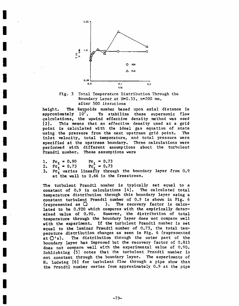
1 I I i i I I 1 1 I I I 1 I 1 I I 1 1

1.01 1

Fig. 3

height . The approximately c a l c u l a t i o n s .

0.0 0.1

Y l t l 0.2

T o t a l Temperature D i s t r i b u t i o n Through t h e Boundary Layer a t N=0.55, x=200 mm, af ter 500 i t e r a t i o n s Rey o l d s number based upon a x i a l d i s t ance is 10 ' . To s t a b i l i z e these supersonic flow

the upwind e f f e c t i v e d e n s i t y method was used [ 2 ] . This means t h a t an e f f e c t i v e dens i ty used a t a g r i d p o i n t is c a l c u l a t e d with t h e i d e a l gas equat ion of state using the pressure from the next u p s t r e a m g r i d point. The in l e t v e l o c i t y , t o t a l temperature, and t o t a l p ressure were s p e c i f i e d a t the upstream boundary. Three c a l c u l a t i o n s were performed with d i f f e r e n t assumptions about t he tu rbu len t P r a n d t l number. These assumptions were

1. Prt = 0.90 Prll = 0.73 2. Pr, = 0.73 Prll = 0.73 3. Prt varies l i n e a r l y through the boundary l a y e r from 0.9

a t the wall t o 0.66 in the freestream.

The t u r b u l e n t P r a n d t l number is t y p i c a l l y set equa l t o a cons tan t of 0.9 i n ca l cu la t ions [41. The c a l c u l a t e d t o t a l temperature d i s t r i b u t i o n through t h i s boundary l a y e r using a cons tan t t u rbu len t P r a n d t l number of 0.9 i s shown in Fig. 6 ( represented as 0 1. The recovery f a c t o r is calcu- l a t e d t o be 0.920 which compares with the empir ica l ly d e t e r mined value of 0.90. However, the d i s t r i b u t i o n of t o t a l temperature through the boundary l a y e r does n o t compare well w i t h the experiment. I f the tu rbu len t P r a n d t l number is set equa l t o the laminar P rand t l number of 0.73, the t o t a l tem- p e r a t u r e d i s t r i b u t i o n changes a s seen i n Fig. 6 ( represented a t 0's). The d i s t r i b u t i o n through the o u t e r p a r t of t he boundary l a y e r has improved b u t the recovery f a c t o r of 0.813 does n o t compare w e l l with the experimental value of 0.90. S c h l i c h t i n g [SI no te s t h a t the tu rbu len t P rand t l number is n o t cons t an t through the boundary l aye r . The experiments of H. Ludwieg [6] f o r turbulent flow through a p i p e show t h a t the P rand t l number varies from approximately 0.9 a t the p i p e

-79-

1 1 I 1 I I D 1 1 I 1 1 I I I I I I 1

Fig. 4 Experimental Total Temperature Distribution in a Flat Plate Turbulent Boundary Layer M=2.8, Rex = 107 after van Driest

Fig.

a c o c o .

Fig.

5

1.0

Geometry and Grid For Boundary Layer Calculations at M=2.8 1

0.96

norm: R.. - 107

0.92

0.38

60 BO LOO 0 20 10

Y I X R

6 Total Temperature Distribution For Flat Plate Boundary Layer at E1=2.8

-80-

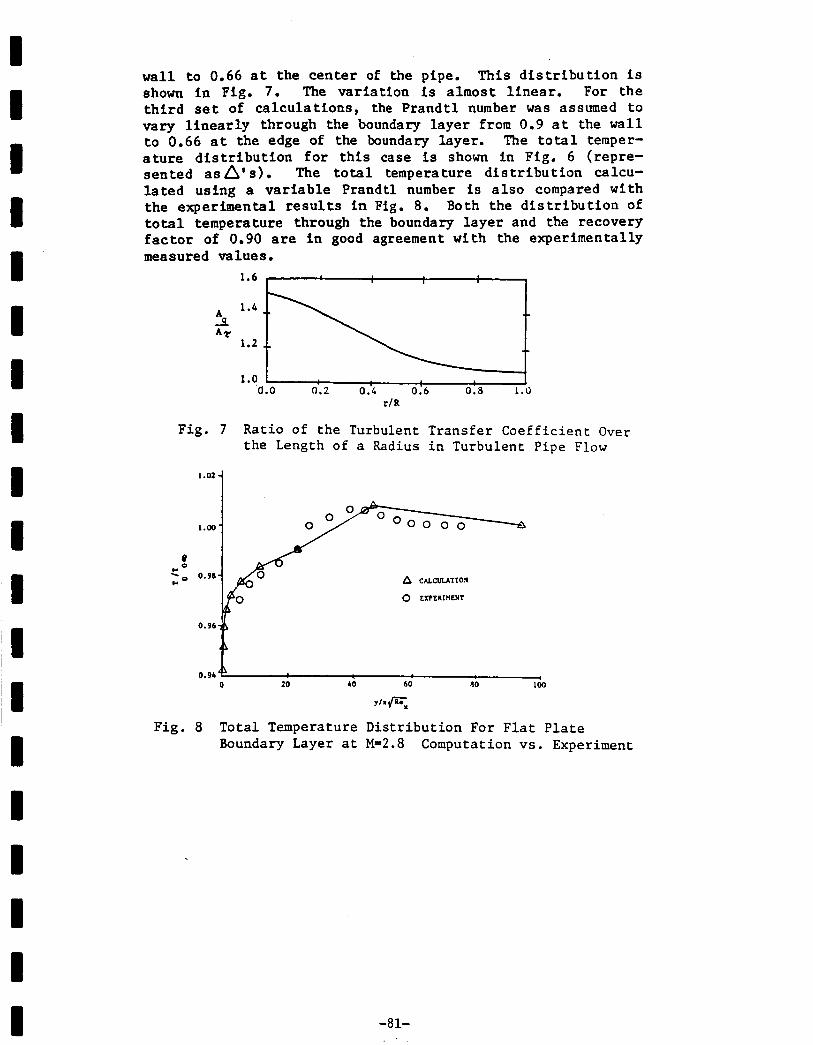
I I I I I I I I I I I ,I ~I I I I I I I

wall t o 0.66 a t the c e n t e r of the pipe. This d i s t r i b u t i o n is ahown in Fig. 7. The v a r i a t i o n is almost l i n e a r . For t h e t h i r d set of c a l c u l a t i o n s , the P rand t l number was assumed t o vary l i n e a r l y through the boundary l a y e r from 0.9 a t the wa l l t o 0.66 a t the edge of the boundary layer . The t o t a l temper- a t u r e d i s t r i b u t i o n f o r t h i s case is shown i n Fig. 6 (repre- s en ted as A's) . The t o t a l temperature d i s t r i b u t i o n ca lcu- l a t e d using a v a r i a b l e Prandt l number is a l s o compared wi th the experimental r e s u l t s i n Fig. 8 . Both the d i s t r i b u t i o n of t o t a l temperature through the boundary l a y e r and the recovery f a c t o r of 0.90 are i n good agreement with the experimental ly measured values.

1.6 i

a.o 0.2 0.4 0 . 6 0.0 1.0 r/R

Fig. 7 Ratio of the Turbulent Transfer Coef f i c i en t Over the Length of a Radius in Turbulent Pipe Flow

1.00

e c o L o

0.98

0.96

0.94 0 20 40 60 no 100

Y h F X

Fig. 8 Tota l Temperature Di s t r ibu t ion For F l a t P la te Boundary Layer a t M=2.8 Computation vs. Experiment

-81-

I I I 1 1 I I I I I I I I I I 1 I 1 I

6 . CONCLUSIONS

A new formulat ion f o r the energy equat ion was introduced which has improved t r a n s i e n t behavior when compared with the s tandard formulation. The new formulation removes the in- f luences of con t inu i ty and momentum e r r o r s from the energy equat ion during t r a n s i e n t s i n the so lu t ion .

For f l a t p l a t e turbulent boundary l a y e r flow with a f rees t ream Mach number of 2.8, the ca l cu la t ed t o t a l tempera- t u r e p r o f i l e was improved by using a v a r i a b l e P rand t l number through boundary layer . The recovery f a c t o r of 0.90 agreed very w e l l with the empir ica l ly determined v a l u e of 0.9.

7 . A(XN0WLEDGEMENTS

This work was supported by NASA Lewis Research Center under NASA Grant NAG 3-593. The au thors are g r a t e f u l t o J e r ry R. Wood and Lou A. Povine l l i f o r t h e i r encouragement and t echn ica l .assis tance.

a.

1.

2.

3.

4.

5.

6.

REFERENCES

NICHOLSON, S., MOORE, J. G., and HOORE, J. - Extension of the F i n i t e Volume Time Marching Method to Laminar and Turbulent Flow. 5 t h In t e rna t iona l Conference on Numeri- cal Methods in Laminar and Turbulent Flow. Ju ly 6-10, 1987, Montreal, Canada. NICHOLSON, S. - Extension of the F i n i t e Volume Pfethod to Laminar and Turbulent Flow. PhD t h e s i s Vi rg in ia Poly- t echn ic I n s t i t u t e and State Universi ty , Blacksburg, VA,

VAN DRIEST, E. R. - Turbulent Boundary Layer i n Compres- 1986.

s i b l e F lu ids , Journa l of the Aeronautical Sciences, Vol. 18, No. 3, March 1951. ANDERSON, D. A., TANNEHILL, J. C., and PLETCHER, R. H. - Computational Fluid Mechanics and Heat Transfer , H e m i s - phere Publ ishing Company, 1984.

SCHLICHTING, H. - Boundary Layer Theory, S ix th Edi t ion , M c G r a w - H i l l , 1968. LUDWIEG, H. - Bestimmung des Verha l tn i sses d e r Austausch- koe f f i z i en ten f u r Watme und Impuls be€ turbulen ten Grenz- schichten. ZFW, 73-81, 1956.

-82-

Documents

OF COLLEGE · OF COLLEGE \liDIIIAlI A VInUIlmlM POLYTECHNIC I~STITUTE UMIVERSITY AND STATE mnlk I I ... Aidpi + i+l + Ai-l'pi-1 +. . . = continuity error, each control volume