Embed Size (px)
Citation preview

Rules & IntegratorsImproper Integrals
Practical Numerical Methods in Physics andAstronomy
Lecture 7 – Numerical Integration II
Pat Scott
Department of Physics, McGill University
February 6, 2013
Slides available fromhttp://www.physics.mcgill.ca/̃ patscott
PHYS 606 Practical Numerical Methods, Winter 2013 Lecture 7 – Numerical Integration II
Rules & IntegratorsImproper Integrals
Recap from last lecture
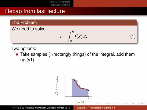
The ProblemWe need to solve
I =
∫ b
af (x)dx (1)
Two options:Take samples (≈rectangly things) of the integral, add themup (v1)
Turn integral equation into different equation, solve that(v2)
PHYS 606 Practical Numerical Methods, Winter 2013 Lecture 7 – Numerical Integration II
Rules & IntegratorsImproper Integrals
Recap from last lecture
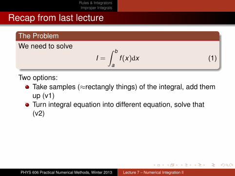
The ProblemWe need to solve
I =
∫ b
af (x)dx (1)
Two options:Take samples (≈rectangly things) of the integral, add themup (v1)
Turn integral equation into different equation, solve that(v2)
PHYS 606 Practical Numerical Methods, Winter 2013 Lecture 7 – Numerical Integration II
Rules & IntegratorsImproper Integrals
Recap from last lecture
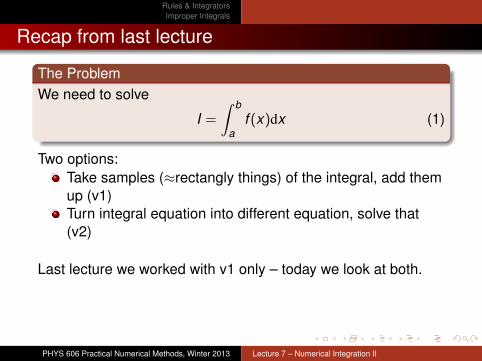
The ProblemWe need to solve
I =
∫ b
af (x)dx (1)
Two options:Take samples (≈rectangly things) of the integral, add themup (v1)Turn integral equation into different equation, solve that(v2)
PHYS 606 Practical Numerical Methods, Winter 2013 Lecture 7 – Numerical Integration II
Rules & IntegratorsImproper Integrals
Recap from last lecture
The ProblemWe need to solve
I =
∫ b
af (x)dx (1)
Two options:Take samples (≈rectangly things) of the integral, add themup (v1)Turn integral equation into different equation, solve that(v2)
Last lecture we worked with v1 only – today we look at both.
PHYS 606 Practical Numerical Methods, Winter 2013 Lecture 7 – Numerical Integration II
Rules & IntegratorsImproper Integrals
Recap from last lecture
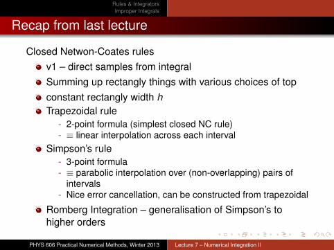
Closed Netwon-Coates rulesv1 – direct samples from integralSumming up rectangly things with various choices of topconstant rectangly width hTrapezoidal rule
- 2-point formula (simplest closed NC rule)- ≡ linear interpolation across each interval
Simpson’s rule- 3-point formula- ≡ parabolic interpolation over (non-overlapping) pairs of
intervals- Nice error cancellation, can be constructed from trapezoidal
Romberg Integration – generalisation of Simpson’s tohigher orders
PHYS 606 Practical Numerical Methods, Winter 2013 Lecture 7 – Numerical Integration II

Rules & IntegratorsImproper Integrals
Today
Solving integrals as DEs (v2)‘Strategic outline’ of how to do itRunge-Kutta as a hand-waving example (RK technicaldetails Wed)
Monte Carlo IntegrationKind of a randomised version of v1
Improper IntegralsWorking with open NC rulesTransforming NC rules for certain integrals
PHYS 606 Practical Numerical Methods, Winter 2013 Lecture 7 – Numerical Integration II

Rules & IntegratorsImproper Integrals
Integration via ODEs and Runge-KuttaMonte Carlo Integration
Outline
1 Rules & IntegratorsIntegration via ODEs and Runge-KuttaMonte Carlo Integration
2 Improper Integrals
PHYS 606 Practical Numerical Methods, Winter 2013 Lecture 7 – Numerical Integration II
Rules & IntegratorsImproper Integrals
Integration via ODEs and Runge-KuttaMonte Carlo Integration
Outline
1 Rules & IntegratorsIntegration via ODEs and Runge-KuttaMonte Carlo Integration
2 Improper Integrals
PHYS 606 Practical Numerical Methods, Winter 2013 Lecture 7 – Numerical Integration II
Rules & IntegratorsImproper Integrals
Integration via ODEs and Runge-KuttaMonte Carlo Integration
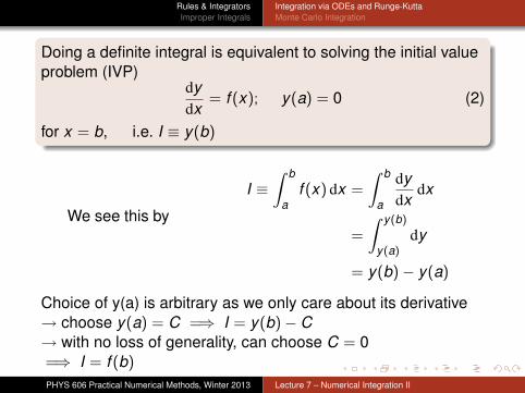
Doing a definite integral is equivalent to solving the initial valueproblem (IVP)
dydx
= f (x); y(a) = 0 (2)
for x = b, i.e. I ≡ y(b)
We see this by
I ≡∫ b
af (x) dx =
∫ b
a
dydx
dx
=
∫ y(b)
y(a)dy
= y(b)− y(a)
Choice of y(a) is arbitrary as we only care about its derivative→ choose y(a) = C =⇒ I = y(b)− C→ with no loss of generality, can choose C = 0=⇒ I = f (b)
PHYS 606 Practical Numerical Methods, Winter 2013 Lecture 7 – Numerical Integration II
Rules & IntegratorsImproper Integrals
Integration via ODEs and Runge-KuttaMonte Carlo Integration
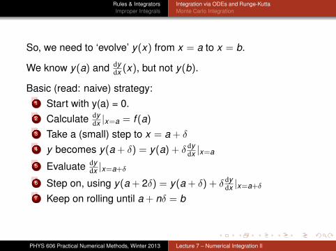
So, we need to ‘evolve’ y(x) from x = a to x = b.
We know y(a) and dydx (x), but not y(b).
Basic (read: naive) strategy:1 Start with y(a) = 0.2 Calculate dy
dx |x=a = f (a)
3 Take a (small) step to x = a + δ
4 y becomes y(a + δ) = y(a) + δ dydx |x=a
5 Evaluate dydx |x=a+δ
6 Step on, using y(a + 2δ) = y(a + δ) + δ dydx |x=a+δ
7 Keep on rolling until a + nδ = b
PHYS 606 Practical Numerical Methods, Winter 2013 Lecture 7 – Numerical Integration II
Rules & IntegratorsImproper Integrals
Integration via ODEs and Runge-KuttaMonte Carlo Integration
So, we need to ‘evolve’ y(x) from x = a to x = b.
We know y(a) and dydx (x), but not y(b).
Basic (read: naive) strategy:1 Start with y(a) = 0.2 Calculate dy
dx |x=a = f (a)
3 Take a (small) step to x = a + δ
4 y becomes y(a + δ) = y(a) + δ dydx |x=a
5 Evaluate dydx |x=a+δ
6 Step on, using y(a + 2δ) = y(a + δ) + δ dydx |x=a+δ
7 Keep on rolling until a + nδ = b
PHYS 606 Practical Numerical Methods, Winter 2013 Lecture 7 – Numerical Integration II

Rules & IntegratorsImproper Integrals
Integration via ODEs and Runge-KuttaMonte Carlo Integration
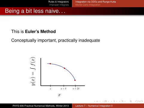
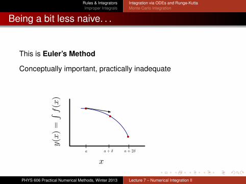
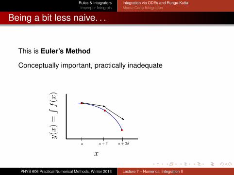
Being a bit less naive. . .
This is Euler’s Method
Conceptually important, practically inadequate
In practice, we need to refine this strategyError checking
How do we know if the derivative has actually stayedroughly constant over δ?
Adaptive step-sizeNeed to adjust δ so evolution is slower (i.e. δ smaller)where dy
dx (x) changes more rapidly
PHYS 606 Practical Numerical Methods, Winter 2013 Lecture 7 – Numerical Integration II
Rules & IntegratorsImproper Integrals
Integration via ODEs and Runge-KuttaMonte Carlo Integration
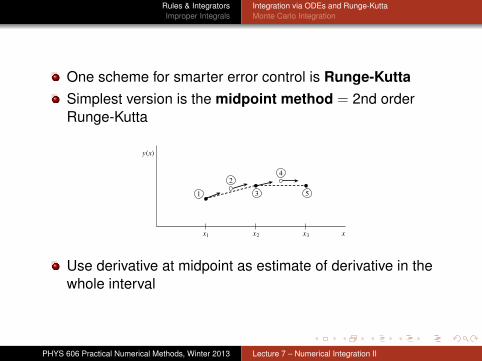
One scheme for smarter error control is Runge-KuttaSimplest version is the midpoint method = 2nd orderRunge-Kutta
y(x)
1
2
x1 x2 x3 x
3
4
5
Use derivative at midpoint as estimate of derivative in thewhole interval
PHYS 606 Practical Numerical Methods, Winter 2013 Lecture 7 – Numerical Integration II
Rules & IntegratorsImproper Integrals
Integration via ODEs and Runge-KuttaMonte Carlo Integration
In doing numerical integration this is not much better thansimply halving the stepsize, because dy
dx does not dependon y (as it does in general ODEs)
Often no need to use full Runge-Kutta – just use Euler’smethod with an appropriately adaptive stepsizerevert to Runge-Kutta if Euler’s method seems to beunstable
Stepsize adaptation can be achieved by e.g.- trying two different δs- compare the results- adjust to smaller stepsize if results differ significantly
(technical details Mon)
PHYS 606 Practical Numerical Methods, Winter 2013 Lecture 7 – Numerical Integration II

Rules & IntegratorsImproper Integrals
Integration via ODEs and Runge-KuttaMonte Carlo Integration
Outline
1 Rules & IntegratorsIntegration via ODEs and Runge-KuttaMonte Carlo Integration
2 Improper Integrals
PHYS 606 Practical Numerical Methods, Winter 2013 Lecture 7 – Numerical Integration II
Rules & IntegratorsImproper Integrals
Integration via ODEs and Runge-KuttaMonte Carlo Integration
Synopsis
I =
∫ b
af (x)dx (3)
Estimate the total area under f (x) by taking random samples off (x) between a and b
Basic Riemann sum is to divide into equal-width rectanglesand sum:
I =b − a
M
M∑i=1
f (xi) (4)
with the xi equally spaced.For large M, Eq. 4 is equally valid if xi are drawn at randombetween a and bFor Monte Carlo integration, the xi are drawn randomlyfrom some distributionW(x)
PHYS 606 Practical Numerical Methods, Winter 2013 Lecture 7 – Numerical Integration II
Rules & IntegratorsImproper Integrals
Integration via ODEs and Runge-KuttaMonte Carlo Integration
Basic Monte Carlo Integration
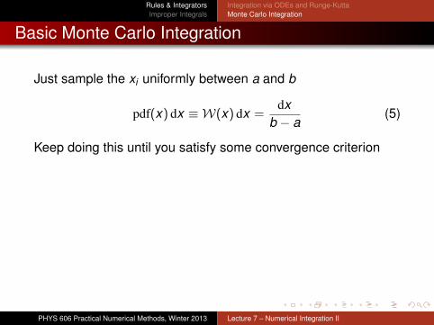
Just sample the xi uniformly between a and b
pdf(x) dx ≡ W(x) dx =dx
b − a(5)
Keep doing this until you satisfy some convergence criterion
Some fixed number of points – easy but looseDouble the number of samples at each step
- compare I with the new set to I with the old (i.e. no overlap)- calculate R = |Inew−Iold|
Inew
- if R < εrequested you’re there: I = 12 (Inew + Iold)
You’re a smart lot – probably you can think of others (dosomething fancy in A3.Q3.a for a bonus mark)
PHYS 606 Practical Numerical Methods, Winter 2013 Lecture 7 – Numerical Integration II
Rules & IntegratorsImproper Integrals
Integration via ODEs and Runge-KuttaMonte Carlo Integration
Basic Monte Carlo Integration
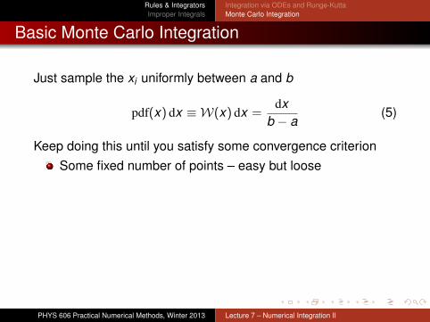
Just sample the xi uniformly between a and b
pdf(x) dx ≡ W(x) dx =dx
b − a(5)
Keep doing this until you satisfy some convergence criterionSome fixed number of points – easy but loose
Double the number of samples at each step- compare I with the new set to I with the old (i.e. no overlap)- calculate R = |Inew−Iold|
Inew
- if R < εrequested you’re there: I = 12 (Inew + Iold)
You’re a smart lot – probably you can think of others (dosomething fancy in A3.Q3.a for a bonus mark)
PHYS 606 Practical Numerical Methods, Winter 2013 Lecture 7 – Numerical Integration II
Rules & IntegratorsImproper Integrals
Integration via ODEs and Runge-KuttaMonte Carlo Integration
Basic Monte Carlo Integration
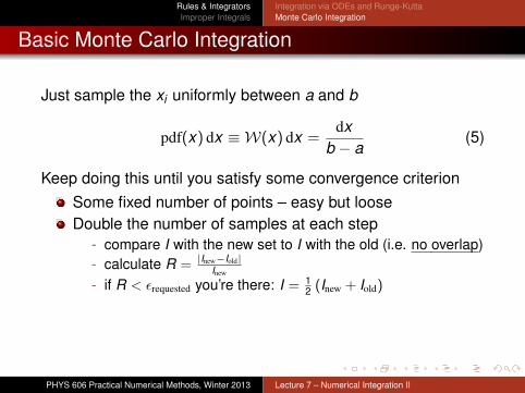
Just sample the xi uniformly between a and b
pdf(x) dx ≡ W(x) dx =dx
b − a(5)
Keep doing this until you satisfy some convergence criterionSome fixed number of points – easy but looseDouble the number of samples at each step
- compare I with the new set to I with the old (i.e. no overlap)- calculate R = |Inew−Iold|
Inew
- if R < εrequested you’re there: I = 12 (Inew + Iold)
You’re a smart lot – probably you can think of others (dosomething fancy in A3.Q3.a for a bonus mark)
PHYS 606 Practical Numerical Methods, Winter 2013 Lecture 7 – Numerical Integration II
Rules & IntegratorsImproper Integrals
Integration via ODEs and Runge-KuttaMonte Carlo Integration
Basic Monte Carlo Integration
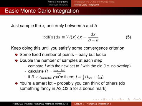
Just sample the xi uniformly between a and b
pdf(x) dx ≡ W(x) dx =dx
b − a(5)
Keep doing this until you satisfy some convergence criterionSome fixed number of points – easy but looseDouble the number of samples at each step
- compare I with the new set to I with the old (i.e. no overlap)- calculate R = |Inew−Iold|
Inew
- if R < εrequested you’re there: I = 12 (Inew + Iold)
You’re a smart lot – probably you can think of others (dosomething fancy in A3.Q3.a for a bonus mark)
PHYS 606 Practical Numerical Methods, Winter 2013 Lecture 7 – Numerical Integration II
Rules & IntegratorsImproper Integrals
Integration via ODEs and Runge-KuttaMonte Carlo Integration
Smarter Monte Carlo Integration – ImportanceSampling
SynopsisAll xi are not created equal – as usual, the louder ones getmore attention
If you have any idea of what your f (x) looks like, choose anon-uniformW(x)
Sample f (x) more densely for those ximportant where f (x) islargest=⇒ they make more contribution to I=⇒ they are more important
PHYS 606 Practical Numerical Methods, Winter 2013 Lecture 7 – Numerical Integration II
Rules & IntegratorsImproper Integrals
Integration via ODEs and Runge-KuttaMonte Carlo Integration
Implementing Importance Sampling
Works best where sampling distributionW(x) is as close aspossible to proportional to f (x)
Must reweight points according to their probability of appearingin our sample
=⇒ I =1M
M∑i=1
f (xi)
W(xi)(6)
PHYS 606 Practical Numerical Methods, Winter 2013 Lecture 7 – Numerical Integration II
Rules & IntegratorsImproper Integrals
Integration via ODEs and Runge-KuttaMonte Carlo Integration
Properly importance-sampled MC integration will convergemuch faster than withoutConvergence tests are similar to with uniform samplingError proportional to M−1/2 for uniform sampling, betterwith a good sampling pdfCompare with error order M−2 for trapezoidal, M−4 forSimpson’s=⇒ MC integration is slow to converge
So why ever use MC integration over other methods??Error always order M−1/2 or better even in n dimensionsTrapezoidal→ M−2/n, Simpson’s→ M−4/n
For higher n, MC integration dominates
PHYS 606 Practical Numerical Methods, Winter 2013 Lecture 7 – Numerical Integration II
Rules & IntegratorsImproper Integrals
Integration via ODEs and Runge-KuttaMonte Carlo Integration
Metropolis-style MC integration
Can do importance sampling via a Markov ChainDraw samples one after another, using the previous to getthe nextRun the typical Metropolis-Hastings step, using thesampling pdf as the objective functionForces sampling density to track the sampling pdf (which isthe whole point, right?)
3 important points to remember1 Gotta have a fixed proposal density2 Gotta have a fixed proposal density3 Remember the difference between the sampling pdf and
the proposal pdf!
PHYS 606 Practical Numerical Methods, Winter 2013 Lecture 7 – Numerical Integration II
Rules & IntegratorsImproper Integrals
Integration via ODEs and Runge-KuttaMonte Carlo Integration
Metropolis-style MC integration
Can do importance sampling via a Markov ChainDraw samples one after another, using the previous to getthe nextRun the typical Metropolis-Hastings step, using thesampling pdf as the objective functionForces sampling density to track the sampling pdf (which isthe whole point, right?)3 important points to remember
1 Gotta have a fixed proposal density2 Gotta have a fixed proposal density3 Remember the difference between the sampling pdf and
the proposal pdf!
PHYS 606 Practical Numerical Methods, Winter 2013 Lecture 7 – Numerical Integration II
Rules & IntegratorsImproper Integrals
Integration via ODEs and Runge-KuttaMonte Carlo Integration
Metropolis-style MC integration
Can do importance sampling via a Markov ChainDraw samples one after another, using the previous to getthe nextRun the typical Metropolis-Hastings step, using thesampling pdf as the objective functionForces sampling density to track the sampling pdf (which isthe whole point, right?)3 important points to remember
1 Gotta have a fixed proposal density
2 Gotta have a fixed proposal density3 Remember the difference between the sampling pdf and
the proposal pdf!
PHYS 606 Practical Numerical Methods, Winter 2013 Lecture 7 – Numerical Integration II
Rules & IntegratorsImproper Integrals
Integration via ODEs and Runge-KuttaMonte Carlo Integration
Metropolis-style MC integration
Can do importance sampling via a Markov ChainDraw samples one after another, using the previous to getthe nextRun the typical Metropolis-Hastings step, using thesampling pdf as the objective functionForces sampling density to track the sampling pdf (which isthe whole point, right?)3 important points to remember
1 Gotta have a fixed proposal density2 Gotta have a fixed proposal density
3 Remember the difference between the sampling pdf andthe proposal pdf!
PHYS 606 Practical Numerical Methods, Winter 2013 Lecture 7 – Numerical Integration II
Rules & IntegratorsImproper Integrals
Integration via ODEs and Runge-KuttaMonte Carlo Integration
Metropolis-style MC integration
Can do importance sampling via a Markov ChainDraw samples one after another, using the previous to getthe nextRun the typical Metropolis-Hastings step, using thesampling pdf as the objective functionForces sampling density to track the sampling pdf (which isthe whole point, right?)3 important points to remember
1 Gotta have a fixed proposal density2 Gotta have a fixed proposal density3 Remember the difference between the sampling pdf and
the proposal pdf!
PHYS 606 Practical Numerical Methods, Winter 2013 Lecture 7 – Numerical Integration II
Rules & IntegratorsImproper Integrals
Integration via ODEs and Runge-KuttaMonte Carlo Integration
Full-blown MCMC integration
Can do full Markov Chain Monte Carlo integration tooRun the typical Metropolis-Hastings step, using f (~x) as theobjective function (instead of someW(~x))Use the fact that the density of points in chain isproportional to the function itselfEssentially importance sampling with the function itself assampling pdfHereW(~x) is equal to f (~x), up to a normalisation factor(which is actually I)Can calculate weights for different points after the fact,using final density of points in that regionThis is how MCMCs and nested sampling estimate theBayesian evidence (multi-D integral over posterior pdf)
PHYS 606 Practical Numerical Methods, Winter 2013 Lecture 7 – Numerical Integration II
Rules & IntegratorsImproper Integrals
Integration via ODEs and Runge-KuttaMonte Carlo Integration
Importance sampling is important (!)
Importance sampling can be used in non-MC integration tooA falling integrand could be sampled more densely near aA strongly-peaked function could be sampled withGaussian intervalsMore complicated integrals could be done on adaptivemeshes (bit of col A, bit of col B)Convergence is optimal when f (~x) is sampled such thateach (hyper-)rectangle contributes ∼equal volume
PHYS 606 Practical Numerical Methods, Winter 2013 Lecture 7 – Numerical Integration II
Rules & IntegratorsImproper Integrals
Outline
1 Rules & IntegratorsIntegration via ODEs and Runge-KuttaMonte Carlo Integration
2 Improper Integrals
PHYS 606 Practical Numerical Methods, Winter 2013 Lecture 7 – Numerical Integration II
Rules & IntegratorsImproper Integrals
Integral decorum
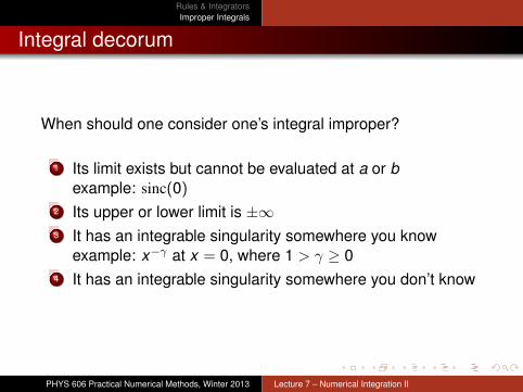
When should one consider one’s integral improper?
1 Its limit exists but cannot be evaluated at a or bexample: sinc(0)
2 Its upper or lower limit is ±∞3 It has an integrable singularity somewhere you know
example: x−γ at x = 0, where 1 > γ ≥ 04 It has an integrable singularity somewhere you don’t know
PHYS 606 Practical Numerical Methods, Winter 2013 Lecture 7 – Numerical Integration II
Rules & IntegratorsImproper Integrals
Coping strategies: dealing with misbehaving integrals
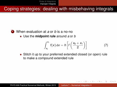
1 When evaluation at a or b is a no-noUse the midpoint rule around a or b∫ x1
x0
f (x) dx = h[f(
x0 + x1
2
)](7)
Stitch it up to your preferred extended closed (or open) ruleto make a compound extended rule
PHYS 606 Practical Numerical Methods, Winter 2013 Lecture 7 – Numerical Integration II
Rules & IntegratorsImproper Integrals
Coping strategies: dealing with misbehaving integrals
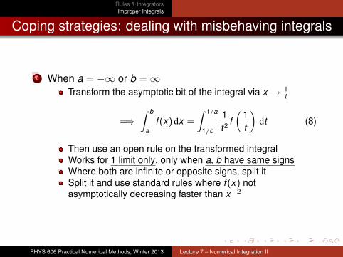
2 When a = −∞ or b =∞Transform the asymptotic bit of the integral via x → 1
t
=⇒∫ b
af (x) dx =
∫ 1/a
1/b
1t2 f(
1t
)dt (8)
Then use an open rule on the transformed integralWorks for 1 limit only, only when a, b have same signsWhere both are infinite or opposite signs, split itSplit it and use standard rules where f (x) notasymptotically decreasing faster than x−2
PHYS 606 Practical Numerical Methods, Winter 2013 Lecture 7 – Numerical Integration II
Rules & IntegratorsImproper Integrals
Coping strategies: dealing with misbehaving integrals
3 When an integrable singularity exists at a known x = xknown
Split the integral so that you have only integrals each withan integrable singularity at one limitTransform the nasty bit of the integral via
x → α, with α = t1
1−γ + a for a singularity near a (9)
α = b − t1
1−γ for a singularity near b (10)
giving ∫ b
af (x) dx =
11− γ
∫ (b−a)1−γ
0t
γ1−γ f (α) dt (11)
(Choose some 0 ≤ γ < 1 of your choice – but best matchedto γ in f (x)→ (x − xnasty)
−γ if this is how your functionbehaves as x → xnasty)Use an open rule on the transformed integral
PHYS 606 Practical Numerical Methods, Winter 2013 Lecture 7 – Numerical Integration II
Rules & IntegratorsImproper Integrals
Coping strategies: dealing with misbehaving integrals
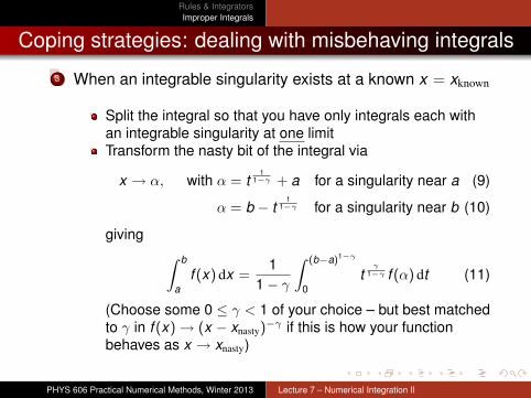
3 When an integrable singularity exists at a known x = xknown
Split the integral so that you have only integrals each withan integrable singularity at one limit
Transform the nasty bit of the integral via
x → α, with α = t1
1−γ + a for a singularity near a (9)
α = b − t1
1−γ for a singularity near b (10)
giving ∫ b
af (x) dx =
11− γ
∫ (b−a)1−γ
0t
γ1−γ f (α) dt (11)
(Choose some 0 ≤ γ < 1 of your choice – but best matchedto γ in f (x)→ (x − xnasty)
−γ if this is how your functionbehaves as x → xnasty)Use an open rule on the transformed integral
PHYS 606 Practical Numerical Methods, Winter 2013 Lecture 7 – Numerical Integration II
Rules & IntegratorsImproper Integrals
Coping strategies: dealing with misbehaving integrals
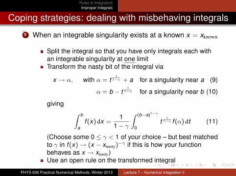
3 When an integrable singularity exists at a known x = xknown
Split the integral so that you have only integrals each withan integrable singularity at one limitTransform the nasty bit of the integral via
x → α, with α = t1
1−γ + a for a singularity near a (9)
α = b − t1
1−γ for a singularity near b (10)
giving ∫ b
af (x) dx =
11− γ
∫ (b−a)1−γ
0t
γ1−γ f (α) dt (11)
(Choose some 0 ≤ γ < 1 of your choice – but best matchedto γ in f (x)→ (x − xnasty)
−γ if this is how your functionbehaves as x → xnasty)
Use an open rule on the transformed integral
PHYS 606 Practical Numerical Methods, Winter 2013 Lecture 7 – Numerical Integration II
Rules & IntegratorsImproper Integrals
Coping strategies: dealing with misbehaving integrals
3 When an integrable singularity exists at a known x = xknown
Split the integral so that you have only integrals each withan integrable singularity at one limitTransform the nasty bit of the integral via
x → α, with α = t1
1−γ + a for a singularity near a (9)
α = b − t1
1−γ for a singularity near b (10)
giving ∫ b
af (x) dx =
11− γ
∫ (b−a)1−γ
0t
γ1−γ f (α) dt (11)
(Choose some 0 ≤ γ < 1 of your choice – but best matchedto γ in f (x)→ (x − xnasty)
−γ if this is how your functionbehaves as x → xnasty)Use an open rule on the transformed integral
PHYS 606 Practical Numerical Methods, Winter 2013 Lecture 7 – Numerical Integration II
Rules & IntegratorsImproper Integrals
Coping strategies: dealing with misbehaving integrals
4 When an integrable singularity exists at an unknown xPrayTry using a variable step size method to find and ‘inch over’the singularity, i.e.
- ODE techniques- Gaussian quadrature- or even MC integration withW(x) somehow peaked around
(unknown!) problem x
PHYS 606 Practical Numerical Methods, Winter 2013 Lecture 7 – Numerical Integration II

Rules & IntegratorsImproper Integrals
Housekeeping
Next lecture Monday (Feb 11)Assignment 2 dueNumerical Solution of ODEs I
PHYS 606 Practical Numerical Methods, Winter 2013 Lecture 7 – Numerical Integration II