Embed Size (px)
Citation preview

Oct. 2006 State-Space Modeling Slide 1
Fault-Tolerant Computing
Motivation, Background, and Tools

Oct. 2006 State-Space Modeling Slide 2
About This Presentation
Edition Released Revised Revised
First Oct. 2006
This presentation has been prepared for the graduate course ECE 257A (Fault-Tolerant Computing) by Behrooz Parhami, Professor of Electrical and Computer Engineering at University of California, Santa Barbara. The material contained herein can be used freely in classroom teaching or any other educational setting. Unauthorized uses are prohibited. © Behrooz Parhami

Oct. 2006 State-Space Modeling Slide 3
State-Space Modeling

Oct. 2006 State-Space Modeling Slide 4
Oct. 2006 State-Space Modeling Slide 5
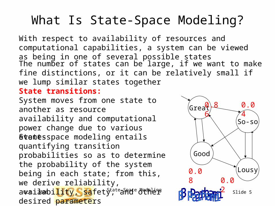
What Is State-Space Modeling?With respect to availability of resources and computational capabilities, a system can be viewed as being in one of several possible states
State transitions:System moves from one state to another as resource availability and computational power change due to various events
State-space modeling entails quantifying transition probabilities so as to determine the probability of the system being in each state; from this, we derive reliability, availability, safety, and other desired parameters
The number of states can be large, if we want to make fine distinctions, or it can be relatively small if we lump similar states together
Great
Lousy
Good
So-so
0.86
0.08
0.04
0.02

Oct. 2006 State-Space Modeling Slide 6
Markov ChainsRepresented by a state diagram with transition probabilities Sum of all transition probabilities out of each state is 1
s(t + 1) = s(t) Ms(t + h) = s(t) M
h
The state of the system is characterized by the vector (s0, s1, s2, s3)(1, 0, 0, 0) means that the system is in state 0(0.5, 0.5, 0, 0) means that the system is in state 0 or 1 with equal prob’s(0.25, 0.25, 0.25, 0.25) represents complete uncertainty
0
3
1
2
0.3
0.5 0.4
0.1
0.30.4
0.1
0.2
Must sum to 1
Transition matrix: M =
0.3 0.4 0.3 00.5 0.4 0 0.1 0 0.2 0.7 0.10.4 0 0.3 0.3
Example:(s0, s1, s2, s3) = (0.5, 0.5, 0, 0) M = (0.4, 0.4, 0.15, 0.05)(s0, s1, s2, s3) = (0.4, 0.4, 0.15, 0.05) M = (0.34, 0.365, 0.225, 0.07)
Markov matrix(rows sum to 1)
Self loops not shown

Oct. 2006 State-Space Modeling Slide 7
Merging States in a Markov Model
011
110
101All solid lines Dashed lines
111 010
100
000
001
33
22
1
0
Failed state if TMR
Simpler equivalent model for 3-unit fail-soft system
Whether or not states are merged depends on the model’s semantics
There are three identical units1 = Unit is up0 = Unit is down

Oct. 2006 State-Space Modeling Slide 8
Two-State Nonrepairable Systems
Reliability as a function of time:R(t) = p1(t) = e–t
Rate of change for the probability of being in state 1 is –p1 = –p1
p1 + p0 = 1
1 0
The label on this transition means that over time dt, the transition will occur with probability dt (we are dealing with a continuous-time Markov model)
p0 = 1 – e–t
p1 = e–t
1
Time
FailureGood FailedStart
State
Initial condition: p1(0) = 1

Oct. 2006 State-Space Modeling Slide 9
k-out-of-n Nonrepairable Systems
n n – 1 n n – 2 (n–1) k k – 1 k… 0 …
pn = –npn
pn–1 = npn – (n – 1)pn–1 ...pk = (k + 1)pk+1 – kpk
pn + pn–1 + . . . + pk + pF = 1
F
pn = e–nt
p1 = ne–(n–1)t(1 – e–t)...pk = ( )e–(n–k)t(1 – e–t)k
pF = 1 – j=k to n pj
nk
Initial condition: pn(0) = 1
In this case, we do not need to resort to more general method of solving linear differential equations (LaPlace transform, to be introduced later)
The first equation is solvable directly, and each additional equation introduces only one new variable

Oct. 2006 State-Space Modeling Slide 10
Two-State Repairable Systems
Availability as a function of time:A(t) = p1(t) = /( + ) + /( + ) e–(+)t
Derived in the next slide
Failure
Up DownStart State
RepairIn steady state (equilibrium), transitions into/out-of each state must “balance out”
–p1 + p0 = 0p1 + p0 = 1
1 0
The label on this transition means that over time dt, repair will occur with probability dt (constant repair rate as well as constant failure rate)
p1 = /( + )p0 = /( + )
1
Steady-state availability
Time

Oct. 2006 State-Space Modeling Slide 11
Solving the State Differential Equations
1 0
To solve linear differential equations with constant coefficients:1. Convert to algebraic equations using LaPlace transform2. Solve the algebraic equations3. Use inverse LaPlace transform to find original solutions
p1(t) = –p1(t) + p0(t) p0(t) = –p0(t) + p1(t)
sP1(s) –p1(0) = –P1(s) + P0(s) sP0(s) –p0(0) = –P0(s) + P1(s)
P1(s) = (s + ) / [s2 + ( + )s]
P0(s) = / [s2 + ( + )s]
1
0
p1(t) = /( + ) + /( + ) e–(+)t
p0(t) = /( + ) – /( + ) e–(+)t
LaPlace Transform Tableh(t) H(s)k k/se–at 1/(s + a)tn–1e–at/(n – 1)! 1/(s + a)n
k h(t) k H(s)h(t) + g(t) H(s) + G(s)h(t) s H(s) – h(0)

Oct. 2006 State-Space Modeling Slide 12
Systems with Multiple Failure States
Safety evaluation:
Total risk of system is failure states cj pj
In steady state (equilibrium), transitions into/out-of each state must “balance out”
–p2 + p1 + p0 = 0–p1 + 1p2 = 0p2 + p1 + p0 = 1
p2 = /( + )p1 = 1/( + )p0 = 0/( + )
GoodStart State
Safe Failed
Unsafe Failed
Failure
Failure
Failure state j has a cost (penalty) cj associated with it
1
2
0
1
0
1 + 0 =
1
Time
p2(t)
p1(t)p0(t)

Oct. 2006 State-Space Modeling Slide 13
Systems with Multiple Operational States
Performability evaluation:
Performability = operational states bj pj
–2p2 + 2p1 = 01p1 – 1p0 = 0p2 + p1 + p0 = 1
p2 = p1 = 2/2
p0 = 12/(12)
Up 2 Up 1Start State
Repair
Failure
Down
Partial repair
Partial failure
Operational state j has a benefit bj associated with it
2
1
2 011
2
Let = 1/[1 + 2/2 + 12/(12)]
Example: 2 = 2, 1 = , 1 = 2 = (single repairperson or facility), b2 = 2, b1 = 1, b0 = 0
P = 2p2 + p1 = 2 + 2/ = 2(1 + /)/(1 +2 / + 22/2)

Oct. 2006 State-Space Modeling Slide 14
TMR System with Repair
Mean time to failure evaluation:See [Siew92], pp. 335-336, for derivationMTTF = 5/(6) + /(62) = [5/(6)](1 + 0.2/)
–3p3 + p2 = 0–( + 2)p2 + 3p3 = 0p3 + p2 + pF = 1
Assume the voter is perfect Upon first module malfunction, we switch to duplex operation with comparison
33 F2 2
Steady-state analysis of no usep3 = p2 = 0, pF = 1
MTTF Comparisons ( = 10–6/hr, = 0.1/hr)Nonredundant 1/ 1 M hrTMR 5/(6) 0.833 M hrTMR with repair [5/(6)](1 + 0.2/) 16,668 M hr
MTTF for TMR
Improvementdue to repair
Improvement factor

Oct. 2006 State-Space Modeling Slide 15
Fail-Soft System with Imperfect Coverage–2p2 + 2p1 = 02(1 – c)p2 + 1p1 – 1p0 = 0p2 + p1 + p0 = 1
p2 = p1 = 2p0 = 2(1 – c + )
Up 2 Up 1Start State
Repair
Failure
Down
Partial repair
Partial failure
If malfunction of one unit goesundetected, the system fails
2c
1
2 011
2
We solve this in the special case of 2 = 2, 1 = , 2 = 1 =
Let = / and = 1 / (1 + 4 – 2c + 22)
We can also consider coverage for the repair direction
2(1 – c)

Oct. 2006 State-Space Modeling Slide 16
Birth-and-Death Processes
Special case of Markov model with states appearing in a chain and transitions allowed only between adjacent states
This model is used in queuing theory, where the customers’ arrival rate and provider’s service rate determine the queue size and waiting timeClosed-form expression for state probabilities can be found, assuming n + 1 states and s service providers (repair persons): M/M/s/n/n queue
pj = (n – j + 1) (/) pj–1 / j for j = 1, 2, . . . , r
pj = (n – j + 1) (/) pj–1 / r for j = r + 1, r + 2, . . . , n
4
0 1
3
23
2 4
2 23
234
Equation for p0
[Siew92], p. 347

Oct. 2006 State-Space Modeling Slide 17
The Dependability Modeling Process
Choose modeling approach Combinational State-space
Solve model
Derive model parameters
Interpret results
Validate model and results
Construct model
Iterate until results are satisfactory

Oct. 2006 State-Space Modeling Slide 18
Software Aids for Reliability Modeling
Relex (company specializing in reliability engineering) Reliability block diagram: http://www.relex.com/products/rbd.asp
Markov: http://www.relex.com/products/markov.asp
Iowa State University HIMAP:
University of Virginia Galileo: http://www.cs.virginia.edu/~ftree/2003-redesign/pages/Software/index.html
See Appendix D, pp. 504-518, of [Shoo02] for more programs
Dept. of Mechanical Engineering, Univ. of Maryland: List of reliability engineering tools: http://www.enre.umd.edu/tools.htm