Ocean TEffH O ICIAl MAGAzINEog Of THE ... - tos.org

CITATION

Engelhart, S.E., B.P. Horton, and A.C. Kemp. 2011. Holocene sea level changes along the United

States’ Atlantic Coast. Oceanography 24(2):70–79, doi:10.5670/oceanog.2011.28.

COPYRIGHT

This article has been published in Oceanography, Volume 24, Number 2, a quarterly journal of

The Oceanography Society. Copyright 2011 by The Oceanography Society. All rights reserved.

USAGE

Permission is granted to copy this article for use in teaching and research. Republication,

systematic reproduction, or collective redistribution of any portion of this article by photocopy

machine, reposting, or other means is permitted only with the approval of The Oceanography

Society. Send all correspondence to: [email protected] or The Oceanography Society, PO Box 1931,

Rockville, MD 20849-1931, USA.

OceanographyTHE OffICIAl MAGAzINE Of THE OCEANOGRAPHY SOCIETY

DOwNlOADED fROM www.TOS.ORG/OCEANOGRAPHY

Oceanography | Vol.24, No.270

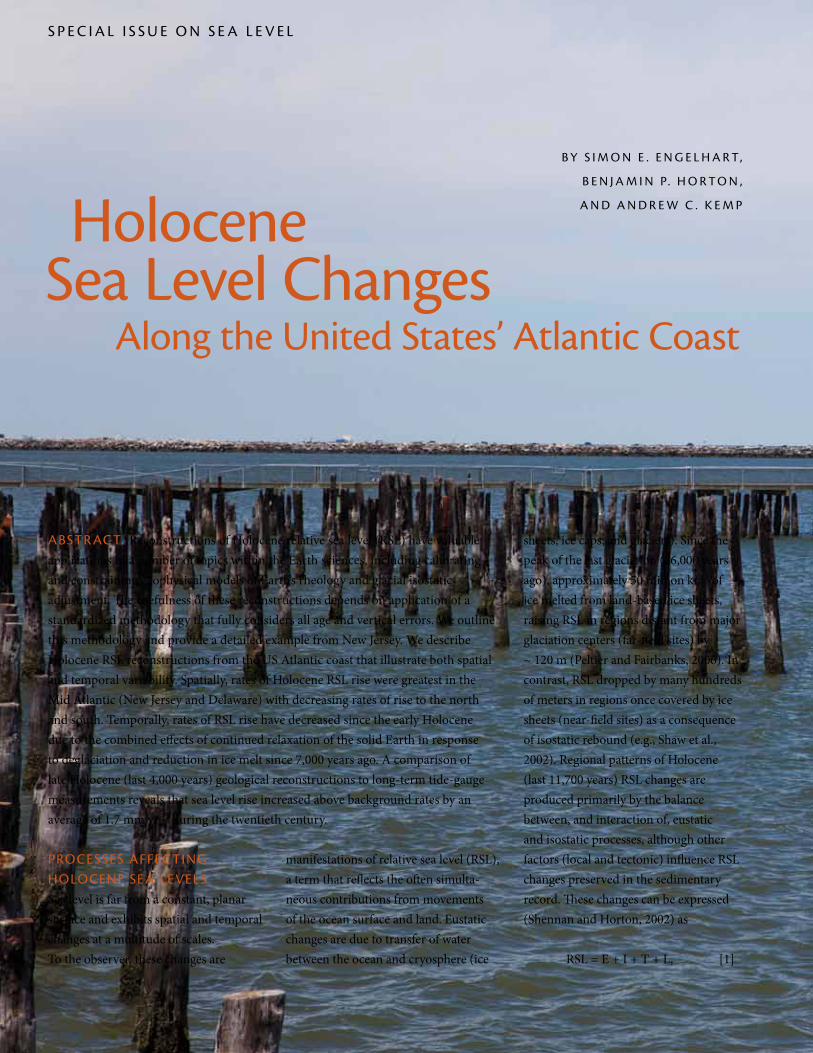
S p e c i a l i S S u e o N S e a l e V e l

HoloceneSea level changes

abStr ac t. Reconstructions of Holocene relative sea level (RSL) have valuable applications in a number of topics within the Earth sciences, including calibrating and constraining geophysical models of Earth’s rheology and glacial isostatic adjustment. The usefulness of these reconstructions depends on application of a standardized methodology that fully considers all age and vertical errors. We outline this methodology and provide a detailed example from New Jersey. We describe Holocene RSL reconstructions from the US Atlantic coast that illustrate both spatial and temporal variability. Spatially, rates of Holocene RSL rise were greatest in the Mid Atlantic (New Jersey and Delaware) with decreasing rates of rise to the north and south. Temporally, rates of RSL rise have decreased since the early Holocene due to the combined effects of continued relaxation of the solid Earth in response to deglaciation and reduction in ice melt since 7,000 years ago. A comparison of late Holocene (last 4,000 years) geological reconstructions to long-term tide-gauge measurements reveals that sea level rise increased above background rates by an average of 1.7 mm yr–1 during the twentieth century.

b y S i m o N e . e N g e l H a r t,

b e N j a m i N p. H o r t o N ,

a N d a N d r e w c . K e m p

along the united States’ atlantic coast

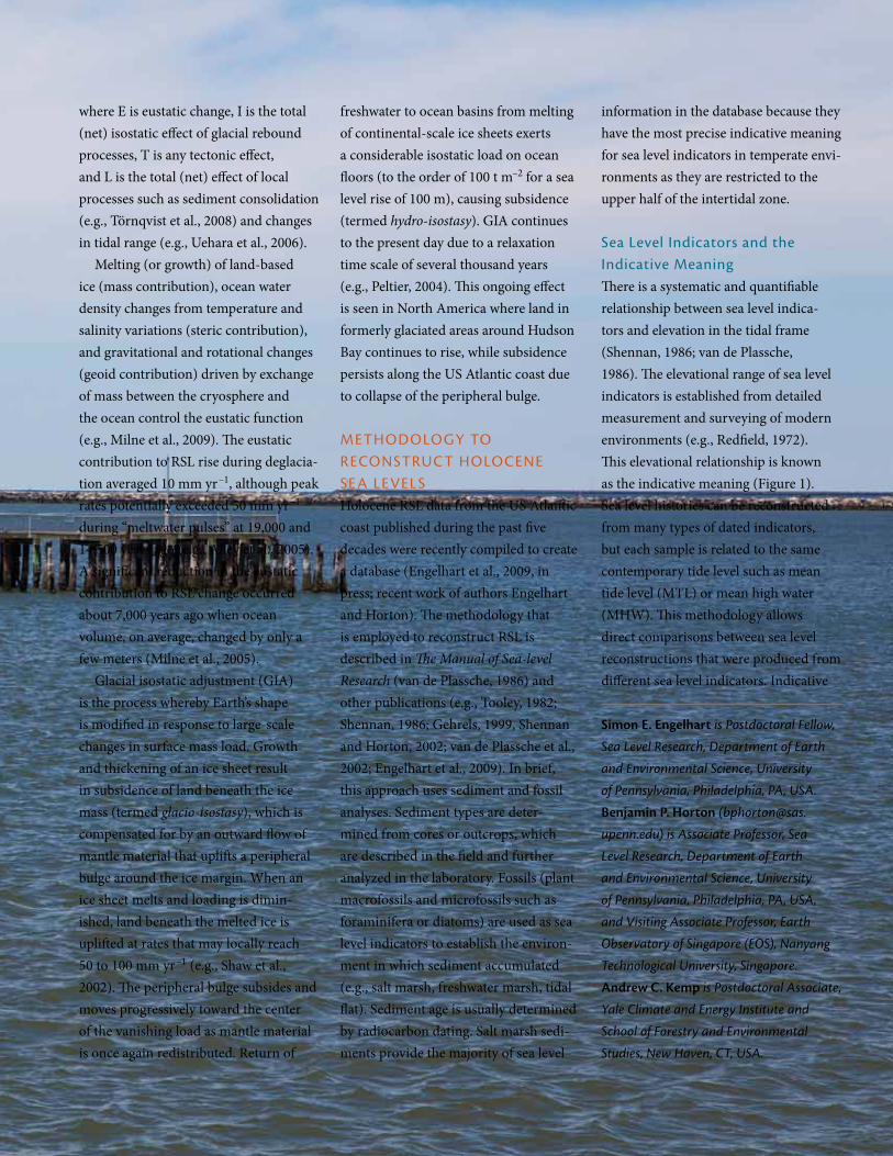
proceSSeS affec tiNg HoloceNe Sea leVelSSea level is far from a constant, planar surface and exhibits spatial and temporal changes at a multitude of scales. To the observer, these changes are

manifestations of relative sea level (RSL), a term that reflects the often simulta-neous contributions from movements of the ocean surface and land. Eustatic changes are due to transfer of water between the ocean and cryosphere (ice

sheets, ice caps, and glaciers). Since the peak of the last glaciation (26,000 years ago), approximately 50 million km3 of ice melted from land-based ice sheets, raising RSL in regions distant from major glaciation centers (far-field sites) by ~ 120 m (Peltier and Fairbanks, 2006). In contrast, RSL dropped by many hundreds of meters in regions once covered by ice sheets (near-field sites) as a consequence of isostatic rebound (e.g., Shaw et al., 2002). Regional patterns of Holocene (last 11,700 years) RSL changes are produced primarily by the balance between, and interaction of, eustatic and isostatic processes, although other factors (local and tectonic) influence RSL changes preserved in the sedimentary record. These changes can be expressed (Shennan and Horton, 2002) as

RSL = E + I + T + L, [1]

Oceanography | june 2011 71

where E is eustatic change, I is the total (net) isostatic effect of glacial rebound processes, T is any tectonic effect, and L is the total (net) effect of local processes such as sediment consolidation (e.g., Törnqvist et al., 2008) and changes in tidal range (e.g., Uehara et al., 2006).

Melting (or growth) of land-based ice (mass contribution), ocean water density changes from temperature and salinity variations (steric contribution), and gravitational and rotational changes (geoid contribution) driven by exchange of mass between the cryosphere and the ocean control the eustatic function (e.g., Milne et al., 2009). The eustatic contribution to RSL rise during deglacia-tion averaged 10 mm yr–1, although peak rates potentially exceeded 50 mm yr–1

during “meltwater pulses” at 19,000 and 14,500 years ago (e.g., Alley et al., 2005). A significant reduction in the eustatic contribution to RSL change occurred about 7,000 years ago when ocean volume, on average, changed by only a few meters (Milne et al., 2005).

Glacial isostatic adjustment (GIA) is the process whereby Earth’s shape is modified in response to large-scale changes in surface mass load. Growth and thickening of an ice sheet result in subsidence of land beneath the ice mass (termed glacio-isostasy), which is compensated for by an outward flow of mantle material that uplifts a peripheral bulge around the ice margin. When an ice sheet melts and loading is dimin-ished, land beneath the melted ice is uplifted at rates that may locally reach 50 to 100 mm yr–1 (e.g., Shaw et al., 2002). The peripheral bulge subsides and moves progressively toward the center of the vanishing load as mantle material is once again redistributed. Return of

freshwater to ocean basins from melting of continental-scale ice sheets exerts a considerable isostatic load on ocean floors (to the order of 100 t m–2 for a sea level rise of 100 m), causing subsidence (termed hydro-isostasy). GIA continues to the present day due to a relaxation time scale of several thousand years (e.g., Peltier, 2004). This ongoing effect is seen in North America where land in formerly glaciated areas around Hudson Bay continues to rise, while subsidence persists along the US Atlantic coast due to collapse of the peripheral bulge.

metHodology to recoNStruc t HoloceNe Sea leVelSHolocene RSL data from the US Atlantic coast published during the past five decades were recently compiled to create a database (Engelhart et al., 2009, in press; recent work of authors Engelhart and Horton). The methodology that is employed to reconstruct RSL is described in The Manual of Sea-level Research (van de Plassche, 1986) and other publications (e.g., Tooley, 1982; Shennan, 1986; Gehrels, 1999, Shennan and Horton, 2002; van de Plassche et al., 2002; Engelhart et al., 2009). In brief, this approach uses sediment and fossil analyses. Sediment types are deter-mined from cores or outcrops, which are described in the field and further analyzed in the laboratory. Fossils (plant macrofossils and microfossils such as foraminifera or diatoms) are used as sea level indicators to establish the environ-ment in which sediment accumulated (e.g., salt marsh, freshwater marsh, tidal flat). Sediment age is usually determined by radiocarbon dating. Salt marsh sedi-ments provide the majority of sea level

information in the database because they have the most precise indicative meaning for sea level indicators in temperate envi-ronments as they are restricted to the upper half of the intertidal zone.

Sea level indicators and the indicative meaningThere is a systematic and quantifiable relationship between sea level indica-tors and elevation in the tidal frame (Shennan, 1986; van de Plassche, 1986). The elevational range of sea level indicators is established from detailed measurement and surveying of modern environments (e.g., Redfield, 1972). This elevational relationship is known as the indicative meaning (Figure 1). Sea level histories can be reconstructed from many types of dated indicators, but each sample is related to the same contemporary tide level such as mean tide level (MTL) or mean high water (MHW). This methodology allows direct comparisons between sea level reconstructions that were produced from different sea level indicators. Indicative

Simon E. Engelhart is Postdoctoral Fellow,

Sea Level Research, Department of Earth

and Environmental Science, University

of Pennsylvania, Philadelphia, PA, USA.

Benjamin P. Horton (bphorton@sas.

upenn.edu) is Associate Professor, Sea

Level Research, Department of Earth

and Environmental Science, University

of Pennsylvania, Philadelphia, PA, USA,

and Visiting Associate Professor, Earth

Observatory of Singapore (EOS), Nanyang

Technological University, Singapore.

Andrew C. Kemp is Postdoctoral Associate,

Yale Climate and Energy Institute and

School of Forestry and Environmental

Studies, New Haven, CT, USA.


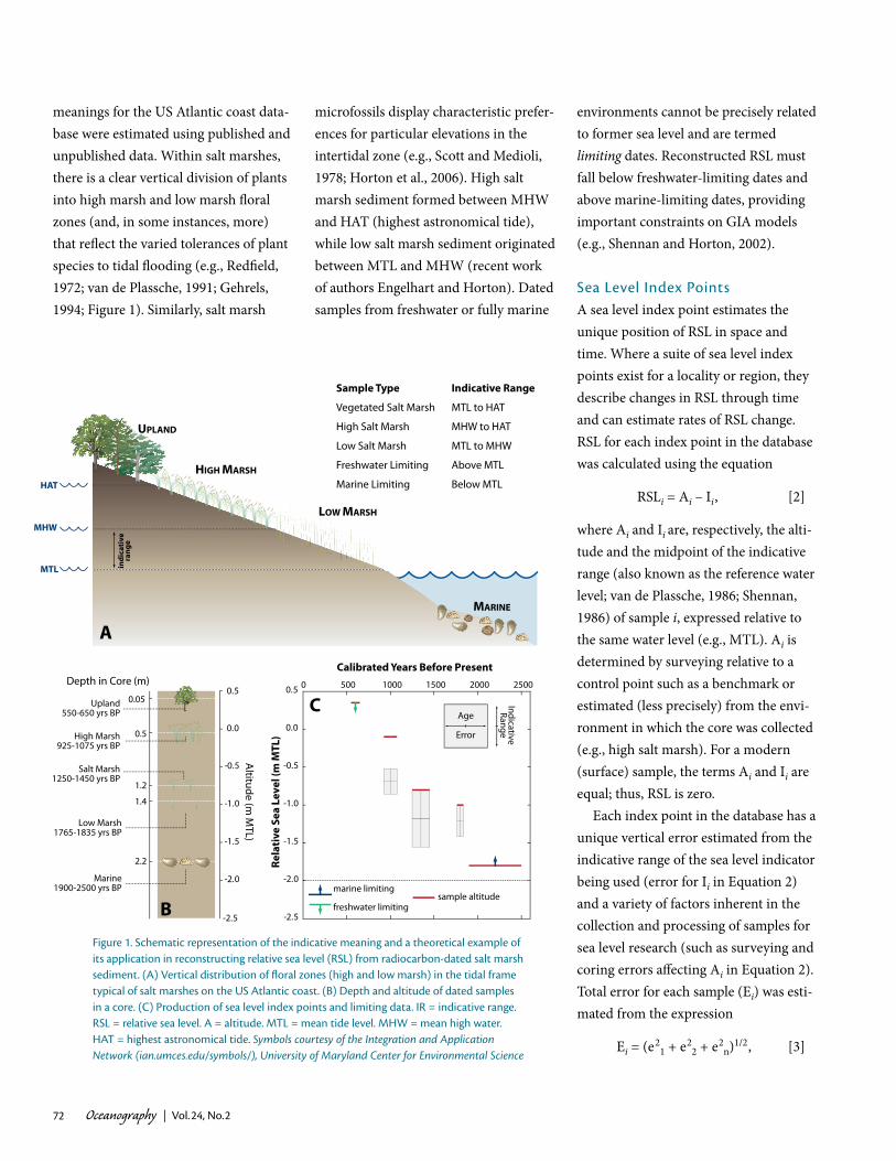
meanings for the US Atlantic coast data-base were estimated using published and unpublished data. Within salt marshes, there is a clear vertical division of plants into high marsh and low marsh floral zones (and, in some instances, more) that reflect the varied tolerances of plant species to tidal flooding (e.g., Redfield, 1972; van de Plassche, 1991; Gehrels, 1994; Figure 1). Similarly, salt marsh

microfossils display characteristic prefer-ences for particular elevations in the intertidal zone (e.g., Scott and Medioli, 1978; Horton et al., 2006). High salt marsh sediment formed between MHW and HAT (highest astronomical tide), while low salt marsh sediment originated between MTL and MHW (recent work of authors Engelhart and Horton). Dated samples from freshwater or fully marine

environments cannot be precisely related to former sea level and are termed limiting dates. Reconstructed RSL must fall below freshwater-limiting dates and above marine-limiting dates, providing important constraints on GIA models (e.g., Shennan and Horton, 2002).

Sea level index pointsA sea level index point estimates the unique position of RSL in space and time. Where a suite of sea level index points exist for a locality or region, they describe changes in RSL through time and can estimate rates of RSL change. RSL for each index point in the database was calculated using the equation

RSLi = Ai – Ii, [2]

where Ai and Ii are, respectively, the alti-tude and the midpoint of the indicative range (also known as the reference water level; van de Plassche, 1986; Shennan, 1986) of sample i, expressed relative to the same water level (e.g., MTL). Ai is determined by surveying relative to a control point such as a benchmark or estimated (less precisely) from the envi-ronment in which the core was collected (e.g., high salt marsh). For a modern (surface) sample, the terms Ai and Ii are equal; thus, RSL is zero.

Each index point in the database has a unique vertical error estimated from the indicative range of the sea level indicator being used (error for Ii in Equation 2) and a variety of factors inherent in the collection and processing of samples for sea level research (such as surveying and coring errors affecting Ai in Equation 2). Total error for each sample (Ei) was esti-mated from the expression

Ei = (e21 + e2

2 + e2n)1/2, [3]

figure 1. Schematic representation of the indicative meaning and a theoretical example of its application in reconstructing relative sea level (rSl) from radiocarbon-dated salt marsh sediment. (a) Vertical distribution of floral zones (high and low marsh) in the tidal frame typical of salt marshes on the uS atlantic coast. (b) depth and altitude of dated samples in a core. (c) production of sea level index points and limiting data. ir = indicative range. rSl = relative sea level. a = altitude. mtl = mean tide level. mHw = mean high water. Hat = highest astronomical tide. Symbols courtesy of the Integration and Application Network (ian.umces.edu/symbols/), University of Maryland Center for Environmental Science

MTL

MHW

HAT

Sample Type Indicative Range

Vegetated Salt Marsh MTL to HAT

High Salt Marsh MHW to HAT

Low Salt Marsh MTL to MHW

Freshwater Limiting Above MTL

Marine Limiting Below MTL

UPLAND

HIGH MARSH

LOW MARSH

indi

cati

vera

nge

0 500 1000 1500 2000 2500

-2.5

-2.0

-1.5

-1.0

-0.5

0.0

0.5

Altitude (m

MTL)

Calibrated Years Before Present

A

Rela

tive

Sea

Lev

el (m

MTL

)

sample altitude

Depth in Core (m)

-2.5

-2.0

-1.5

-1.0

-0.5

0.0

0.50.05

0.5

1.2

1.4

2.2

Upland550-650 yrs BP

High Marsh925-1075 yrs BP

Salt Marsh1250-1450 yrs BP

Low Marsh1765-1835 yrs BP

Marine1900-2500 yrs BP

B

C

freshwater limiting

marine limiting

Age

Error

IndicativeRange

MARINE


where e1…en are individual sources of error for sample i (Shennan and Horton, 2002).

Another source of vertical error in sea level reconstruction is sediment consolidation from reduction of sedi-ment volume by rearrangement of the mineral matrix and biodegradation (Kaye and Barghoorn, 1964). No error term was estimated for this factor. Sediment consolidation serves to lower the altitude of a sea level index point (Ai in Equation 2) below that at which it was initially deposited. This process can

result in an RSL reconstruction that is too low (Figure 2). Methods to estimate (and thus potentially correct for) consol-idation (e.g., Brain et al., 2011) require quantitative information about the type of sediment above and below the dated sample, which was not available for many sea level index points.

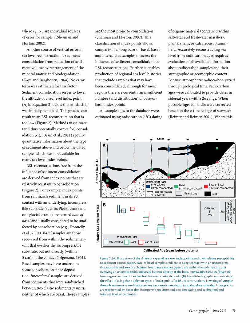
RSL reconstructions free from the influence of sediment consolidation are derived from index points that are relatively resistant to consolidation (Figure 2). For example, index points from salt marsh sediment in direct contact with an underlying, incompress-ible substrate (such as Pleistocene sand or a glacial erratic) are termed base of basal and usually considered to be unaf-fected by consolidation (e.g., Donnelly et al., 2004). Basal samples are those recovered from within the sedimentary unit that overlies the incompressible substrate, but not directly (within 5 cm) on the contact (Jelgersma, 1961). Basal samples may have undergone some consolidation since deposi-tion. Intercalated samples are derived from sediments that were sandwiched between two clastic sedimentary units, neither of which are basal. These samples

are the most prone to consolidation (Shennan and Horton, 2002). This classification of index points allows comparison among base-of-basal, basal, and intercalated samples to assess the influence of sediment consolidation on RSL reconstructions. Further, it enables production of regional sea level histories that exclude samples that may have been consolidated, although for most regions there are currently an insufficient number (and distribution) of base-of-basal index points.

All sample ages in the database were estimated using radiocarbon (14C) dating

of organic material (contained within saltwater and freshwater marshes), plants, shells, or calcareous foramin-ifera. Accurately reconstructing sea level from radiocarbon ages requires evaluation of all available information about radiocarbon samples and their stratigraphic or geomorphic context. Because atmospheric radiocarbon varied through geological time, radiocarbon ages were calibrated to provide dates in sidereal years with a 2σ range. When possible, ages for shells were corrected based on the estimated age of seawater (Reimer and Reimer, 2001). Where this

Intercalated (likely compacted)

Basal (maybe compacted)

Base of Basal (likely uncompacted)

Incompressiblesubstrate Silt and clay Peat

Index Point Type

Rela

tive

Sea

Lev

el (m

MTL

)

Calibrated Age (years before present)

Alt

itud

e (m

MTL

)

Calib. Age

ErrorRSL

Indi

cativ

e Ra

nge

and

othe

r alti

tudi

nal

erro

rs

Base of BasalBasalIntercalated

Index Point Type

Cores

A

B

figure 2. (a) illustration of the different types of sea level index points and their relative susceptibility to sediment consolidation. base-of-basal samples (red) are in direct contact with an uncompress-ible substrate and are consolidation free. basal samples (green) are within the sedimentary unit overlying an uncompressible substrate but not directly at the base. intercalated samples (blue) are from organic sediment sandwiched between clastic deposits. (b) age-altitude graph demonstrating the effect of using these different types of index points for rSl reconstructions. lowering of samples through sediment consolidation serves to overestimate depth (and therefore altitude). index points are represented by boxes that incorporate age (from radiocarbon dating and calibration) and total sea level uncertainties.


information was not available, the stan-dard marine reservoir correction value was used (e.g., Hughen et al., 2004). All sea level index points were presented as calibrated years before present (BP), where year 0 is conventionally taken to be AD 1950 (Stuiver and Polach, 1977).

example of data collected: a late Holocene basal Sea level index point from New jerseyWe use an example from New Jersey to illustrate the methodology used to create a sea level index point.

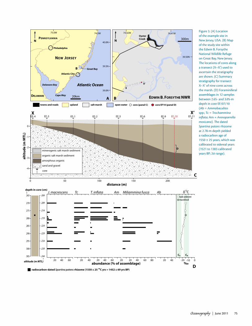
Core EF/07/10 (39.49°N, 74.42°W) was collected from a salt marsh at Edwin B. Forsythe National Wildlife Refuge in New Jersey on the US mid-Atlantic coast (Figure 3A). Presently, tidal range (mean lower low water [MLLW] to mean higher high water [MHHW]) at the site is 1.10 m. The modern marsh is dominated by stunted salt marsh cordgrass (Spartina alterniflora) with patchy presence of seashore saltgrass (Distichlis spicata) and salt meadow cordgrass (Spartina patens). Transects of cores across the marsh (Figure 3B) revealed that the organic-rich sediments deposited at the site overlie an incompressible substrate of glacial outwash sands and gravels. The salt-marsh-derived sediment was less than 0.3-m thick at the salt marsh/terrestrial boundary and increased to more than 4 m at the most seaward core.

Core-top altitude was established by leveling (± 0.05-m leveling error using a total station) to a National Geodetic Survey benchmark with first order vertical precision (± 0.10-m benchmark error). Its surface altitude was 0.48 m above North American Vertical Datum (NAVD88; converted to 0.61 m above MTL using data reported for the tide

gauge at Atlantic City; Figure 3). The bottom of the core was 3.89 m below MTL. From –3.59 to –2.19 m MTL, the core was composed of organic sediment and contained sparse remains of identifi-able plant fossils. In contrast, organic sediment in the upper 2.8 m of the core (–2.19 to 0.61 m MTL) contained large numbers of identifiable high salt marsh plant remains. Agglutinated foraminifera were present in the upper 3.95 m of the core. A Spartina patens rhizome with a known relationship (e.g., van de Plassche et al., 1998) to the former marsh surface (0.01 m thick; ± 0.01-m sampling error) was selected for dating. It was found 2.78 m below the surface (± 0.03-m bore-hole error) at –2.17 m MTL. It yielded a radiocarbon age of 1550 ± 25 14C years and date of 1521–1383 calibrated years BP (2σ range). Samples were analyzed for foraminifera to verify the environment of deposition (Figure 3D). Samples from –2.39 to –2.22 m MTL were dominated by the agglutinated foraminifera Miliammina fusca with occurrences of Jadammina macrescens. Foraminifera between –2.20 and –2.09 m were indicative of a high salt marsh environment as illustrated by high abundances of Tiphotrocha comprimata and Trochammina inflata. The plant remains and foraminifera suggest that the radiocarbon-dated sample formed in a high salt marsh environment. Therefore, the dated sample was assigned an indicative range of MHW to HAT (0.86 m MTL ± 0.25 m). The sample lies within a basal organic sedimentary unit of amorphous and salt marsh peat that overlies an incompressible substrate of sand and gravel. It was not sampled within 0.05 m of the boundary and thus is considered a basal rather than a

base-of-basal index point. The calculation of RSL and associated

error term for this index point was

RSL = –2.17 m MTL – 0.86 m MTL = –3.03 m MTLError = Σ(0.25 m2

indicative range + 0.005 m2

thickness + 0.05 m2

levelling + 0.01 m2

sampling + 0.1 m2

benchmark + 0.03 m2

borehole)1/2 = ± 0.28 mAge = 1550 ± 25 14C years = 1,521–1,383 calibrated years BP

(2σ range)

tHe uS atl aNtic coaSt databaSe of Sea leVel iNdex poiNtSThe database included 70 fields of infor-mation from which conditional filters (such as possible contamination, erosion of sediment contact, stratigraphical context, and type of radiocarbon measurement) were applied to define sea level index points that we believed to be reliably related to past tide levels. This procedure produced 473 Holocene sea level index points, of which 75 were categorized as base of basal, 267 as basal, and 131 as intercalated. Additionally, 158 freshwater-limiting dates and 189 marine-limiting dates were produced. The database covered more than 1,800 km of coastline from Maine to South Carolina (Figure 4). No validated sea level index points were available for Georgia and Florida. Following Engelhart et al. (in press) and recent work of authors Engelhart and Horton, the Holocene database was divided into 16 regions (Figures 4 and 5). GIA was the principal cause of spatial


Delaware Bay

NEW JERSEY

Philadelphia

Atlantic City

Atlantic Ocean

B

20km

39.5N

39.0N

40.0N

74.5W75.0W

PENNSYLVANIA

DELAWARE

N 300mOysterCreekN

B

74.42W 74.41W

39.50N

open waterupland salt marshtowns and roads

Great Bay

Cape May EDWIN B. FORSYTHE NWR

265

270

275

280

285

290

295

300

30520 40 60 20 40 20 40 60 20 20 40 60 80 20 40 -20 0-10

J. macrescens T. in�ataTc Am Miliammina fusca Ab

abundance (% of assemblage) ‰

δ C13

A

C3 C4

D

depth in core (cm)

altitude (m MTL)

core (panel C) core EF10 (panel D)

radiocarbon-dated Spartina patens rhizome (1550 ± 25 14C yrs = 1452 ± 69 yrs BP)

X X’

distance (m)0 50 100 150 200

amorphous organic

organic salt marsh sediment

minerogenic salt marsh sediment

sand and gravel

core

C

EF-4 EF-3 EF-1 EF-2 EF-5 EF-6 EF-9 EF-10 EF-11

D

alti

tude

(m M

TL)

bulk sedimentmacrofossil

-204

-244

-209

-239

-214

-234

-219

-229

-224

0

-1

-2

-3

-4

X

X’

figure 3. (a) location of the example site in New jersey, uSa. (b) map of the study site within the edwin b. forsythe National wildlife refuge on great bay, New jersey. The locations of cores along a transect (x–x’) used to ascertain the stratigraphy are shown. (c) Summary stratigraphy for transect x–x’ of nine cores across the marsh. (d) foraminiferal assemblages in 12 samples between 2.65- and 3.05-m depth in core ef/07/10 (ab = Ammobaculites spp.; tc = Trochammina inflata; am = Arenoparrella mexicana). The dated Spartina patens rhizome at 2.78-m depth yielded a radiocarbon age of 1550 ± 25 years, which was calibrated to sidereal years (1521 to 1383 calibrated years bp; 2σ range).


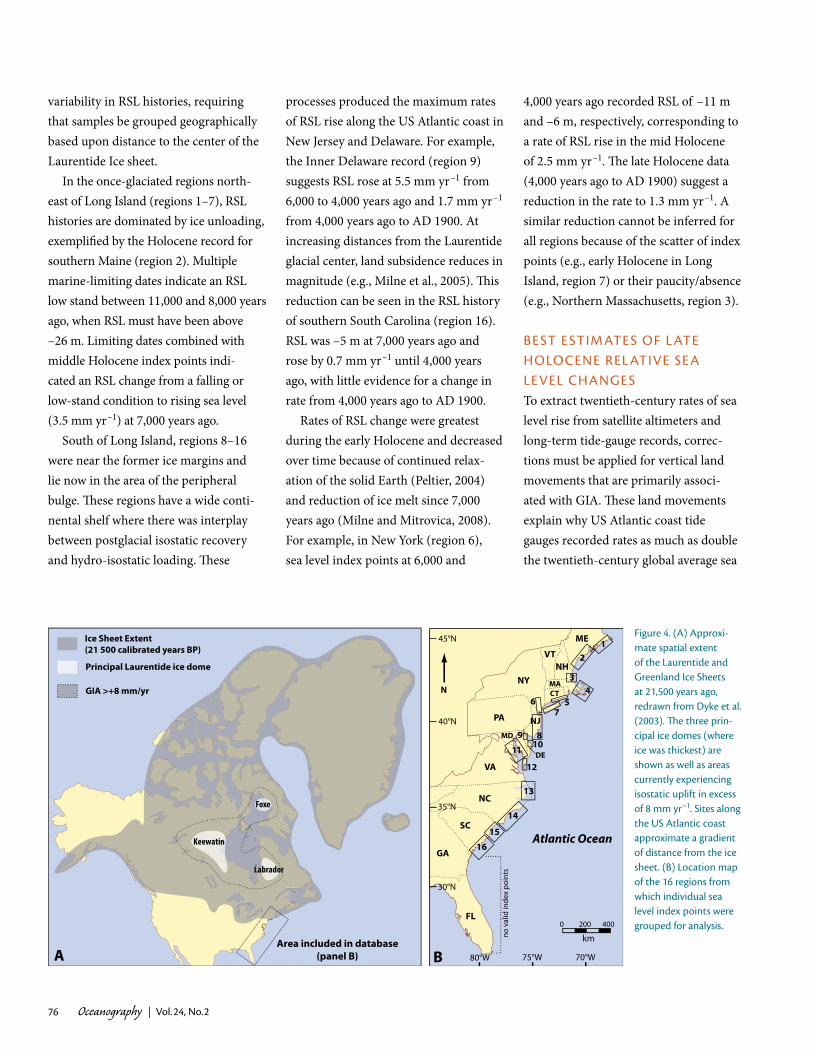
variability in RSL histories, requiring that samples be grouped geographically based upon distance to the center of the Laurentide Ice sheet.

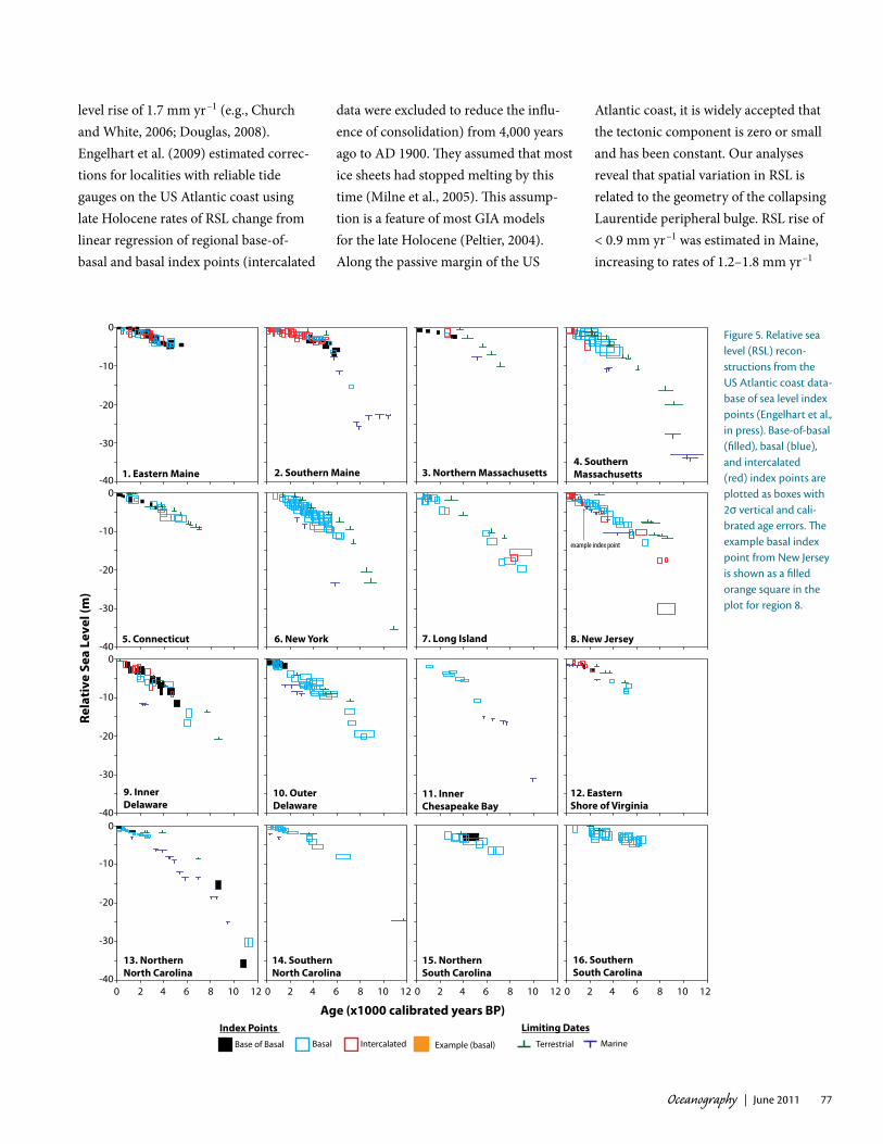
In the once-glaciated regions north-east of Long Island (regions 1–7), RSL histories are dominated by ice unloading, exemplified by the Holocene record for southern Maine (region 2). Multiple marine-limiting dates indicate an RSL low stand between 11,000 and 8,000 years ago, when RSL must have been above –26 m. Limiting dates combined with middle Holocene index points indi-cated an RSL change from a falling or low-stand condition to rising sea level (3.5 mm yr–1) at 7,000 years ago.

South of Long Island, regions 8–16 were near the former ice margins and lie now in the area of the peripheral bulge. These regions have a wide conti-nental shelf where there was interplay between postglacial isostatic recovery and hydro-isostatic loading. These

processes produced the maximum rates of RSL rise along the US Atlantic coast in New Jersey and Delaware. For example, the Inner Delaware record (region 9) suggests RSL rose at 5.5 mm yr–1 from 6,000 to 4,000 years ago and 1.7 mm yr–1 from 4,000 years ago to AD 1900. At increasing distances from the Laurentide glacial center, land subsidence reduces in magnitude (e.g., Milne et al., 2005). This reduction can be seen in the RSL history of southern South Carolina (region 16). RSL was –5 m at 7,000 years ago and rose by 0.7 mm yr–1 until 4,000 years ago, with little evidence for a change in rate from 4,000 years ago to AD 1900.

Rates of RSL change were greatest during the early Holocene and decreased over time because of continued relax-ation of the solid Earth (Peltier, 2004) and reduction of ice melt since 7,000 years ago (Milne and Mitrovica, 2008). For example, in New York (region 6), sea level index points at 6,000 and

4,000 years ago recorded RSL of –11 m and –6 m, respectively, corresponding to a rate of RSL rise in the mid Holocene of 2.5 mm yr–1. The late Holocene data (4,000 years ago to AD 1900) suggest a reduction in the rate to 1.3 mm yr–1. A similar reduction cannot be inferred for all regions because of the scatter of index points (e.g., early Holocene in Long Island, region 7) or their paucity/absence (e.g., Northern Massachusetts, region 3).

beSt eStimateS of l ate HoloceNe rel atiVe Sea leVel cHaNgeSTo extract twentieth-century rates of sea level rise from satellite altimeters and long-term tide-gauge records, correc-tions must be applied for vertical land movements that are primarily associ-ated with GIA. These land movements explain why US Atlantic coast tide gauges recorded rates as much as double the twentieth-century global average sea

km

0 400200

45°N

40°N

30°N

80°W 75°W 70°W

Atlantic Ocean

ME

NY MACT

NJPA

MD

DE

VA

NC

SC

GA

FL

35°N

12

34

567

8910

11

12

14

16

B

15

13

NHVT

no v

alid

inde

x po

ints

N

Ice Sheet Extent(21 500 calibrated years BP)

Area included in database(panel B)A

Principal Laurentide ice dome

GIA >+8 mm/yr

Keewatin

Labrador

Foxe

figure 4. (a) approxi-mate spatial extent of the laurentide and greenland ice Sheets at 21,500 years ago, redrawn from dyke et al. (2003). The three prin-cipal ice domes (where ice was thickest) are shown as well as areas currently experiencing isostatic uplift in excess of 8 mm yr–1. Sites along the uS atlantic coast approximate a gradient of distance from the ice sheet. (b) location map of the 16 regions from which individual sea level index points were grouped for analysis.


level rise of 1.7 mm yr–1 (e.g., Church and White, 2006; Douglas, 2008). Engelhart et al. (2009) estimated correc-tions for localities with reliable tide gauges on the US Atlantic coast using late Holocene rates of RSL change from linear regression of regional base-of-basal and basal index points (intercalated

data were excluded to reduce the influ-ence of consolidation) from 4,000 years ago to AD 1900. They assumed that most ice sheets had stopped melting by this time (Milne et al., 2005). This assump-tion is a feature of most GIA models for the late Holocene (Peltier, 2004). Along the passive margin of the US

Atlantic coast, it is widely accepted that the tectonic component is zero or small and has been constant. Our analyses reveal that spatial variation in RSL is related to the geometry of the collapsing Laurentide peripheral bulge. RSL rise of < 0.9 mm yr–1 was estimated in Maine, increasing to rates of 1.2–1.8 mm yr–1

0

-10

-20

-30

-400

-10

-20

-30

-400

-10

-20

-30

-400

-10

-20

-30

-400 2 4 6 8 10 12 0 2 4 6 8 10 12 0 2 4 6 8 10 12 0 2 4 6 8 10 12

Age (x1000 calibrated years BP)Index Points Limiting Dates

Base of Basal Basal Intercalated Terrestrial Marine

1. Eastern Maine 2. Southern Maine 3. Northern Massachusetts4. SouthernMassachusetts

5. Connecticut 6. New York 7. Long Island 8. New Jersey

9. InnerDelaware

10. OuterDelaware

11. InnerChesapeake Bay

12. EasternShore of Virginia

13. NorthernNorth Carolina

14. SouthernNorth Carolina

15. NorthernSouth Carolina

16. SouthernSouth Carolina

Rela

tive

Sea

Lev

el (m

)

example index point

Example (basal)

figure 5. relative sea level (rSl) recon-structions from the uS atlantic coast data-base of sea level index points (engelhart et al., in press). base-of-basal (filled), basal (blue), and intercalated (red) index points are plotted as boxes with 2σ vertical and cali-brated age errors. The example basal index point from New jersey is shown as a filled orange square in the plot for region 8.


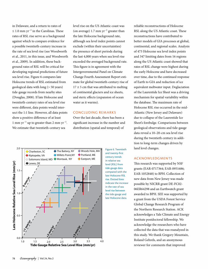
in Delaware, and a return to rates of ≤ 1.0 mm yr–1 in the Carolinas. These rates of RSL rise serve as a background against which to compare evidence for a possible twentieth-century increase in the rate of sea level rise (see Woodworth et al., 2011, in this issue, and Woodworth et al., 2009). In addition, these back-ground rates of RSL will be critical for developing regional predictions of future sea level rise. Figure 6 compares late Holocene trends of RSL estimated from geological data with long (> 50 years) tide-gauge records from nearby sites (Douglas, 2008). If late Holocene and twentieth-century rates of sea level rise were different, data points would inter-sect the 1:1 line. However, all data points show a positive difference of at least 1 mm yr–1 up to greater than 2 mm yr–1. We estimate that twentieth-century sea

level rise on the US Atlantic coast was (on average) 1.7 mm yr–1 greater than the late Holocene background rate, although sea level index points cannot exclude (within their uncertainties) the presence of short periods during the last 4,000 years when sea level rise exceeded the averaged background rate. This figure is in agreement with the Intergovernmental Panel on Climate Change Fourth Assessment Report esti-mate for global twentieth-century rise of 17 ± 5 cm that was attributed to melting of continental glaciers and ice sheets, and steric effects (expansion of ocean water as it warms).

coNcludiNg remarKSOver the last decade, there has been a significant increase in the number and distribution (spatial and temporal) of

reliable reconstructions of Holocene RSL along the US Atlantic coast. These reconstructions have contributed to better models of GIA processes at global, continental, and regional scales. Analysis of 473 Holocene sea level index points and 347 limiting dates from 16 regions along the US Atlantic coast showed that rates of RSL change were highest during the early Holocene and have decreased over time, due to the continued response of Earth to GIA and reduction of ice equivalent meltwater input. Deglaciation of the Laurentide Ice Sheet was a driving mechanism for spatial variability within the database. The maximum rate of Holocene RSL rise occurred in the mid-Atlantic (New Jersey and Delaware) due to collapse of the Laurentide Ice Sheet’s forebulge. Comparisons between geological observations and tide-gauge data reveal a 10–20-cm sea level rise during the twentieth century in addi-tion to long-term changes driven by land level changes.

acKNowledgmeNtSThis research was supported by NSF grants (EAR-0717364; EAR-0951686; EAR-1052848) to BPH. Collection of new data from New Jersey was made possible by NICRR grant DE-FC02-06ER64298 and an Earthwatch grant awarded to BPH. SEE was supported by a grant from the USDA Forest Service Global Change Research Program of the Northern Research Station. ACK acknowledges a Yale Climate and Energy Institute postdoctoral fellowship. We acknowledge the researchers who have collected the data that was reanalyzed in this study. We thank Gregory Mountain, Roland Gehrels, and an anonymous reviewer for comments that improved Tide Gauge Relative Sea Level Rise (mm/yr)

Late

Hol

ocen

e Re

lati

ve S

ea L

evel

Ris

e (m

m/y

r)

Charleston, SCKiptopeke, VASolomons Island, MDLewes, DE

The Battery, NYWillets Point,NYMontauk, NY

Woods Hole, MAPortland, MEEastport, ME

0 m

m/y

r

+1 m

m/y

r

+2 m

m/y

r

+3 m

m/y

r

2.0

1.5

1.0

0.5

0.01.0 1.5 2.0 2.5 3.0 3.5 4.0

figure 6. twentieth and twenty-first century trends in relative sea level (rSl) from tide-gauge data compared with the late Holocene rSl rise. dotted lines indicate the increase in the rate of sea level rise between the tide-gauge and late Holocene data.


the manuscript. This paper is a contribu-tion to IGCP Project 588 and PALSEA, and is Earth Observatory of Singapore (EOS) publication number #25.

refereNceSAlley, R.B., P.U. Clark, P. Huybrechts, and

I. Joughin. 2005. Ice-sheet and sea-level changes. Science 310:456–460.

Brain, M.J., A.J. Long, D.N. Petley, B.P. Horton, and R.J. Allison. 2011. Compression behaviour of minerogenic low energy intertidal sediments. Sedimentary Geology 23:28–41, doi:10.1016/ j.sedgeo.2010.10.005.

Church, J.A., and N.J. White. 2006. A 20th century acceleration in global sea-level rise. Geophysical Research Letters 33, L01602, doi:10.1029/2005GL024826.

Donnelly, J.P., P. Cleary, P. Newby, and R. Ettinger. 2004. Coupling instrumental and geological records of sea-level change: Evidence from southern New England of an increase in the rate of sea-level rise in the late 19th century. Geophysical Research Letters 31, L05203, doi:10.1029/2003GL018933.

Douglas, B.C. 2008. Concerning evidence for fingerprints of glacial melting. Journal of Coastal Research 24:218–227, doi:10.2112/06-0748.1.

Dyke, A.S., A. Moore, and L. Robertson. 2003. Deglaciation of North America. Geological Survey of Canada Open File 1574.

Engelhart, S.E., B.P. Horton, B.C. Douglas, W.R. Peltier, and T.E. Tornqvist. 2009. Spatial variability of late Holocene and 20th century sea-level rise along the Atlantic coast of the United States. Geology 37:1,115–1,118.

Engelhart, S.E., W.R. Peltier, and B.P. Horton. In press. Holocene relative sea-level changes and glacial isostatic adjustment of the US Atlantic coast. Geology.

Gehrels, W.R. 1994. Determining relative sea-level change from salt-marsh foraminifera and plant zones on the coast of Maine, USA. Journal of Coastal Research 10:990–1,009.

Gehrels, W.R. 1999. Middle and late Holocene sea-level changes in Eastern Maine reconstructed from foraminiferal saltmarsh stratigraphy and AMS C-14 dates on basal peat. Quaternary Research 52:350–359.

Horton, B.P., R. Corbett, S.J. Culver, R.J. Edwards, and C. Hillier. 2006. Modern saltmarsh diatom distributions of the Outer Banks, North Carolina, and the development of a transfer function for high resolution reconstructions of sea level. Estuarine, Coastal and Shelf Science 69:381–394.

Hughen, K., M. Baillie, E. Bard, A. Bayliss, J. Beck, C. Bertrand, P. Blackwell, C. Buck, G. Burr, and K. Cutler. 2004. Marine04 marine radio-carbon age calibration, 26-0 ka BP. Radiocarbon 46:1,059–1,086.

Jelgersma, S. 1961. Holocene sea-level changes in the Netherlands. Mededelingen Geologische Stichting Serie C 7:1–100.

Kaye, C.A., and E.S. Barghoorn. 1964. Late Quaternary sea-level change and crustal rise at Boston, Massachusetts, with notes on the autocompaction of peat. Geological Society of America Bulletin 75:63–80.

Milne, G.A., and J.X. Mitrovica. 2008. Searching for eustasy in deglacial sea-level histories. Quaternary Science Reviews 27:2,292–2,302.

Milne, G.A., W.R. Gehrels, C.W. Hughes, and M.E. Tamisiea. 2009. Identifying the causes of sea-level change. Nature Geoscience 2:471–478.

Milne, G.A., A.J. Long, and S.E. Bassett. 2005. Modelling Holocene relative sea-level observa-tions from the Caribbean and South America. Quaternary Science Reviews 24:1,183–1,202.

Peltier, W.R. 2004. Global glacial isostasy and the surface of the ice-age Earth: The ice-5G (VM2) model and GRACE. Annual Review of Earth and Planetary Sciences 32:111–149.

Peltier, W.R., and R.G. Fairbanks. 2006. Global glacial ice volume and Last Glacial Maximum duration from an extended Barbados sea level record. Quaternary Science Reviews 25:3,322–3,337.

Redfield, A.C. 1972. Development of a New England salt marsh. Ecological Monographs 42:201–237.

Reimer, P., and R. Reimer. 2001. A marine reservoir correction database and on-line interface. Radiocarbon 43:461–463.

Scott, D.S., and F.S. Medioli. 1978. Vertical zona-tions of marsh foraminifera as accurate indica-tors of former sea-levels. Nature 272:528–531.

Shaw, J., P. Gareau, and R.C. Courtney. 2002. Palaeogeography of Atlantic Canada 13–0 kyr. Quaternary Science Reviews 21:1,861–1,878.

Shennan, I. 1986. Flandrian sea-level changes in the Fenland. II. Tendencies of sea-level movement, altitudinal changes, and local and regional factors. Journal of Quaternary Science 1:155–179.

Shennan, I., and B. Horton. 2002. Holocene land- and sea-level changes in Great Britain. Journal of Quaternary Science 17:511–526.

Stuiver, M., and H.A. Polach. 1977. Discussion: Reporting of 14C data. Radiocarbon 19:355–363.

Tooley, M.J. 1982. Sea-level changes in northern England. Proceedings of the Geologists’ Association 93:43–51, doi:10.1016/S0016- 7878(82)80031-X.

Törnqvist, T.E., D.J. Wallace, J.E.A. Storms, J. Wallinga, R.L. Van Dam, M. Blaauw, M.S. Derksen, C.J.W. Klerks, C. Meijneken,

and E.M.A. Snijders. 2008. Mississippi Delta subsidence primarily caused by compaction of Holocene strata. Nature Geoscience 1:173–176.

Uehara, K., J. Scourse, K. Horsburgh, K. Lambeck, and A. Purcell. 2006. Tidal evolution of the northwest European shelf seas from the Last Glacial Maximum to the present. Journal of Geophysical Research 111, C09025, doi:10.1029/2006JC003531.

van de Plassche, O. 1986. Sea-level Research: A Manual for the Collection and Evaluation of Data. Kluwer Academic Publishers, 618 pp.

van de Plassche, O., ed. 1991. Late Holocene sea-level fluctuations on the shore of Connecticut inferred from transgressive and regressive overlap boundaries in salt-marsh deposits. Journal of Coastal Research special issue 11:159–179.

van de Plassche, O., K. van der Borg, and A.F.M. de Jong. 1998. Sea level-climate correlation during the past 1400 yr. Geology 26:319–322.

van de Plassche, O., K. van der Borg, and A.F.M. de Jong. 2002. Relative sea-level rise across the Eastern Border fault (Branford, Connecticut): Evidence against seismotectonic movements. Marine Geology 184:61–68.

Woodworth, P.L., W.R. Gehrels, and R.S. Nerem. 2011. Nineteenth and twentieth century changes in sea level. Oceanography 24(2):80–93, doi:10.5670/oceanog.2011.29.

Woodworth, P.L., N.J. White, S. Jevrejeva, S.J. Holgate, J.A. Church, and W.R. Gehrels. 2009. Evidence for the accelerations of sea level on multi-decade and century timescales. International Journal of Climatology 29:777–789.

Documents

Ocean TEffH O ICIAl MAGAzINEog Of THE ... - tos.org