Earth Planets Space, 58, 429–437, 2006

Ocean circulation generated magnetic signals

C. Manoj1,2, A. Kuvshinov3,4, S. Maus1,5, and H. Luhr1

1GeoForchungsZentrum-Potsdam, Germany2National Geophysical Research Institute, Hyderabad, India

3Danish National Space Center, Copenhagen, 2100, Denmark4Geoelectromagnetic Research Institute, Troitsk, Russia

5NOAA’s National Geophysical Data Center, Boulder, U.S.A.

(Received November 15, 2004; Revised March 29, 2005; Accepted April 21, 2005; Online published April 14, 2006)

Conducting ocean water, as it flows through the Earth’s magnetic field, generates secondary electric and mag-netic fields. An assessment of the ocean-generated magnetic fields and their detectability may be of impor-tance for geomagnetism and oceanography. Motivated by the clear identification of ocean tidal signatures in theCHAMP magnetic field data we estimate the ocean magnetic signals of steady flow using a global 3-D EM nu-merical solution. The required velocity data are from the ECCO ocean circulation experiment and alternativelyfrom the OCCAM model for higher resolution. We assume an Earth’s conductivity model with a surface thinshell of variable conductance with a realistic 1D mantle underneath. Simulations using both models predict anamplitude range of ±2 nT at Swarm altitude (430 km). However at sea level, the higher resolution simulationpredicts a higher strength of the magnetic field, as compared to the ECCO simulation. Besides the expectedsignatures of the global circulation patterns, we find significant seasonal variability of ocean magnetic signals inthe Indian and Western Pacific Oceans. Compared to seasonal variation, interannual variations produce weakersignals.Key words: Ocean flow, geomagnetic field, satellite measurements.

1. IntroductionAs the conducting water in the ocean moves in the am-

bient geomagnetic field of the Earth, it induces secondaryelectric and magnetic fields. This phenomenon is a case ofmotional induction, where the electrically charged ions inthe sea water are deflected by the Lorentz force perpendic-ular to both the velocity and magnetic field vectors (Tyleret al., 2003). The spatial charge accumulation causes elec-tric currents within the conducting water and bottom sedi-ments. Based on the geometry of these currents, the oceaninduced magnetic fields may be classified into “toroidal”and “poloidal”. The toroidal components are caused byelectric currents closing in the vertical plane and have anamplitude range of 10 to 100 nT and are confined to theocean and the upper crust. The poloidal components arisefrom the electrical currents closing in the horizontal planeand have a much smaller amplitude range (1 to 10 nT) at thesea level. However its large spatial decay scale allows thepoloidal fields to reach outside the ocean to remote land andsatellite based sensors. The poloidal magnetic field compo-nents, observed outside the ocean are mainly proportionalto the depth integrated velocities (transport) of the ocean(Tyler et al., 1999). The possibility of identifying the oceanmagnetic signals on land and satellite based magnetometerrecords have two implications. The ocean magnetic sig-nals can give information about the major water transport

Copyright c© The Society of Geomagnetism and Earth, Planetary and Space Sci-ences (SGEPSS); The Seismological Society of Japan; The Volcanological Societyof Japan; The Geodetic Society of Japan; The Japanese Society for Planetary Sci-ences; TERRAPUB.

across the oceans and their variability (Vivier et al., 2004).On the other hand, the non trivial contribution of oceanmagnetic signals to the geomagnetic field necessitates ac-counting for them in geomagnetic field modeling (e.g. Mauset al., 2005).

Faraday (1832) was the first to recognize the motionalinduction in sea water. Larsen (1968) and Sanford (1971)were the modern day pioneers in the investigation of theocean generated electric fields. The effect of the ocean dy-namics, coastline and the electrical structure of the Earthon the induced electromagnetic fields were discussed byChave (1983). Attempts to estimate ocean induced elec-tric and/or magnetic fileds with realistic ocean circulationmodels have been made by Stephenson and Bryan (1992),Flosadottir et al. (1997a,b), Tyler et al. (1997, 1999) andPalshin et al. (1999). Recently Vivier et al. (2004) corre-lated the variation in the simulated magnetic fields with thewater transport across the Drake Passage. The predictedelectric and/or magnetic fields were validated by under-sea-cable voltage measurements (cf. Larsen and Sanford,1985), land based electrical or magnetic field measurements(Junge, 1988; Maus and Kuvshinov, 2004), sea floor or seasurface magnetic field measurements (Lilley et al., 2004a,b)and satellite magnetic measurements (Tyler et al., 2003).

The use of satellite magnetic data is particularly promis-ing, considering their global coverage, and the small spa-tial decay scale of the ocean magnetic signals. The oceangenerated magnetic field has a typical strength of 1 nT atCHAMP satellite altitude. To separate such signals fromthe observed magnetic signal (of a typical strength 50,000

429

430 C. MANOJ et al.: OCEAN MAGNETIC SIGNALS

nT) is not a trivial task. However, with the advancementin the technology to measure and process the satellite mag-netic data, it is now possible to identify the tidal magneticsignals in CHAMP data (Tyler et al., 2003). The low fre-quency magnetic signals produced by the quasi-stationaryocean circulations may be more difficult to separate as com-pared to tidal magnetic signals. However the Swarm mis-sion, which intends to measure the Earth’s magnetic fieldat an unprecedented precision promises to detect the oceanmagnetic signals associated with ocean circulation. This pa-per details the result of the simulations carried out to assessthe detectability of ocean magnetic signals with the Swarmmission. The primary objectives of the simulation were 1)To assess the large scale as well as small scale magneticfield effects of the ocean circulation at sea level and satellitealtitude and 2) to examine their temporal variability. In ad-dition, characterizing the ocean magnetic signals is an im-portant first step in trying to identify the ocean magnetic sig-nals in the satellite magnetic data. The first part of the paperdiscusses the forward computation, i.e. the electromagneticnumerical solution and the ocean circulation models usedfor the simulation. The results from the forward computa-tion are discussed in the second part. The temporal varia-tions of the ocean magnetic signals are treated in the lastpart of the paper.

2. Forward Computation of Ocean Magnetic Sig-nals

In order to calculate the magnetic fields due to globalocean steady flow, we have adopted the numerical solutionwhich is described in Kuvshinov et al. (2002, 2005) andwhich has been already successfully applied for ocean tidalsignals simulations (Maus and Kuvshinov, 2004; Kuvshi-nov and Olsen, 2005). The solution is based on a volumeintegral equation approach, which combines the modifiediterative dissipative method (MIDM; Singer, 1995) witha conjugate gradients iteration. The solution allows sim-ulating the electromagnetic (EM) fields, excited by arbi-trary sources in three-dimensional (3-D) spherical modelsof electric conductivity. These models consist of a numberof anomalies of 3-D conductivity, embedded in a host sec-tion of radially symmetric (1-D) conductivity. Within thisapproach Maxwell’s equations in the frequency domain,

∇ × H = σE + jext , (1)

∇ × E = iωµoH, (2)

are reduced, in accordance with the MIDM, to a scatteringequation of specific type (Pankratov et al., 1997)

χ(r) −∫

V mod

K (r, r′)R(r′)χ(r′)dv′ = χo(r), (3)

which is solved by the generalized bi-conjugate gradientmethod (Zhang, 1997). In the equations above jext is theexciting current, its time-harmonic dependency is e−iωt , µo

is the magnetic permeability of free space, i = √−1, ω =2π/T is the angular frequency, T is the period of variations,σ(r, ϑ, ϕ) is the conductivity distribution in the model, ϑ, ϕ

and r are co-latitude, longitude and the distance from the

Earth’s centre, respectively, r = (r, ϑ, ϕ), r′ = (r ′, ϑ ′, ϕ′),V mod is the modelling region, and

R = σ − σo

σ + σo(4)

K (r, r′) = δ(r − r′)I + 2√

σo(r)Geo(r, r′)

√σo(r ′), (5)

χo =∫

V mod

K (r, r′)√

σo

σ + σojs(r′)dv′, (6)

χ = 1

2√

σo((σ + σo)Es + js), (7)

js = (σ − σo)Eo, (8)

Eo =∫

V ext

Geo(r, r′)jext (r′)dv′. (9)

Here δ(r − r′) is Dirac’s delta function, I is the identity op-erator, V ext is the volume occupied by the exciting currentjext , Es = E − Eo is the scattered electric field, Ge

o is the3 × 3 dyadic Green’s function of the 1-D reference conduc-tivity σo(r).

Once χ is determined from the solution of the scatter-ing equation (3), the magnetic field, H, at the observationpoints, r ∈ V obs (in our case V obs is the surface of the Earth)is calculated as

H =∫

V ext

Gho(r, r′)jext (r′)dv′ +

∫

V mod

Gho(r, r′)jq(r′)dv′,

(10)with

jq = (σ − σo)(Eo + Es), (11)

Es = 1

σ + σo(2

√σoχ − js). (12)

Explicit expressions for the elements of Geo and Gh

o aregiven in the appendix of Kuvshinov et al. (2002). Havingthe magnetic field at the surface of the Earth one can re-calculate the magnetic field at the satellite altitude, using aspherical decomposition of the magnetic fields calculated atthe surface of the Earth.

As the present study focuses on the steady state oceanflow, the period of simulation is set to a large value. Sinceour 3-D conductivity model of the Earth consists of a sur-face spherical shell of S(θ, ϕ) underlain by a radially sym-metric conductor, jext reduces to the sheet current density,Jext

τ , which is calculated as

Jextτ = σw(U × er Bm

r ), (13)

where × denotes the vector product, σw = 3.2 S/m is themean sea water conductivity, U is the depth integrated ve-locity of global steady ocean flow, er is the outward unitvector and Bm

r is the radial component of the main mag-netic field derived from a model IGRF 2000. The shellconductance S(ϑ, ϕ) consists of contributions from the seawater and from sediments. The conductance of the seawater has been derived from the ocean salinity, tempera-ture and pressure data given by World Ocean Atlas 2001(www.nodc.noaa.gov), following the formulations by Fo-fonoff (1985). Conductance of the sediments is based on

C. MANOJ et al.: OCEAN MAGNETIC SIGNALS 431

the global sediment thickness given by the 1◦ × 1◦ mapof Laske and Masters (1997) and calculated by a heuristicprocedure similar to that described in Everett et al. (2003).Figure 1 presents the map of the surface shell conductanceof 0.25◦ × 0.25◦ resolution. For the underlying sphericalconductor we choose a four-layer Earth model (similar tothat described in Schmucker, 1985) instead of assuming aninsulating mantle (cf. Vivier et al., 2004). It consists of a100 km resistive lithosphere with 3000 � m followed by amoderately resistive first layer of 70 �m down to 500 km,a second transition layer of 16 �m from 500 km to 750km, and an inner uniform sphere of 0.42 �m. Each simu-lation (with ECCO velocity data) took 1.2 hours CPU timeon one processor of the type SunFire V8800 for a modeldiscretization of Nθ × Nφ = 180 × 360 and with an angu-lar resolution of 1◦ × 1◦. When simulating magnetic fieldsbased on the OCCAM data, using a model discretization ofNθ × Nφ = 720 × 1440 and with an angular resolution of0.25◦ × 0.25◦, it took 20 hours for the same processor.2.1 Ocean circulation models

We obtained the velocity data for the forward compu-tations from two ocean circulation models viz. ECCO(http://www.ecco-group.org) and OCCAM (http://www.soc.soton.ac.uk/JRD/OCCAM). The ECCO (Estimatingthe Circulation and Climate of the Ocean) model is based onthe MIT general circulation model (Marshall et al., 1997).We use the data from the ECCO 1 model run (1992 to2002). Using a model adjoint approach, the ECCO 1 modelwas forced to be consistent with the World Ocean Circu-lation Experiment (WOCE) observations. The model runwas configured globally with a 1◦ × 1◦ horizontal resolu-tion, within ±80◦ latitudes and with 23 levels in the verti-cal. The horizontal components of the velocity data were in-terpolated to a common grid and were vertically integratedto obtain the transport data. The monthly transport gridsfrom January 1992 to December 2002 were used to simu-late the ocean magnetic signals. Additionally, the data froma high resolution ocean model OCCAM (Ocean Circulationand Climate Advance Modeling) were used to simulate themagnetic field effects of the ocean eddies. The model has36 levels in the vertical starting with a thickness of 20 mat the surface and increasing to 250 m at depth. The spa-tial resolution of the model is 0.25◦ × 0.25◦ (Webb et al.,1998). Archived OCCAM velocity data are available forevery 15 days for most of the analysis period within the lat-itudinal limits +66◦ to −77◦. However, velocity data arenot available for the North Atlantic Ocean region. For theSwarm simulations we used the average horizontal velocityfields from the 2985 and 3000 days of the OCCAM modelrun. Figure 2 shows the magnitude distribution of velocitydata from both models. Basically, both models describe themajor features of the ocean flow in a similar way. How-ever ocean eddies are resolved only by the OCCAM model.For OCCAM data, the missing data for the North AtlanticOcean region were filled with ECCO data.

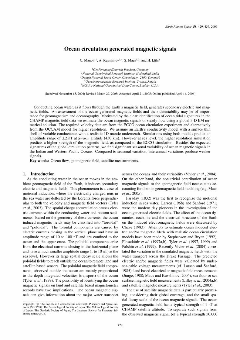
3. ResultsThe radial components of the predicted magnetic field

(Br ) from ECCO and OCCAM data are presented in theFig. 3. The dominant ocean induced magnetic signal is

the radial component, Br and the horizontal componentshave about half of that strength. We do not plot other com-ponents, as all fields are poloidal, the horizontal fields donot contain additional information. At sea level (bottompanels), both predictions are within the amplitude range±10 nT and look quite similar. However on closer in-spection, high-intensity and short-wavelength features aremore evident in OCCAM simulations. The maxima andminima of magnetic fields are 4 nT and −6 nT for ECCOand ±10 nT for OCCAM simulations. The effect of oceaneddies is clearly visible in the Kuroshio Current regionand along the Antarctic Circumpolar Current (ACC) region.These effects are by and large, absent in the ECCO simula-tions. Arguably, the smaller but intense flows resolved bythe OCCAM model resulted in stronger magnetic signals atsea level. However, at satellite altitude (430 km) the pre-dicted magnetic fields only contain information about thelarge scale features of the ocean circulation. Both predic-tions are within the amplitude range ±2 nT. The mag-netic fields from ECCO data have a slightly higher ampli-tude above the ACC in the Southern Indian Ocean (ECCO:−1.5 nT and OCCAM: −1.2 nT) at satellite altitude. Bothsimulations are predominantly influenced by the ACC andWestern boundary currents. The eastward flowing ACC re-sults in two prominent anomalies to the east and west of thesouthern geomagnetic pole (located in the South AustralianOcean). The predicted amplitudes of the magnetic fields atsatellite altitude are in agreement with the computations byTyler et al. (1999).3.1 Magnetic field effect of ocean eddies

A detailed map of the Kuroshio Current region is givenin Fig. 4. The bottom panel shows the radial componentof the predicted magnetic field at sea level, and the upperpanel the magnetic field at satellite altitude. Both maps aresuperimposed on the velocity vectors from the OCCAM re-sults. The induced magnetic fields due to eddies are evi-dent at sea level, with a large amplitude range of ±10 nT.These anomalies can be considered as a compounded effectof magnetic fields generated by individual eddies. As theocean-continent boundary represents a large lateral contrastin conductance, the variation in sensitivity of the magneticfields with respect to the conductance also must be takeninto account. The one-to-one relationships between eddiesand predicted anomalies are difficult to explain consideringthese complications. At satellite altitude the magnetic fieldsof individual eddies are not resolved (upper panel of Fig. 4).Here, the magnetic signatures of the Kuroshio Current existas smooth elongated anomalies running parallel to the coast.This result stress the need to use a high resolution (and eddyresolving) ocean model while looking for the ocean signalsin the magnetic records from the land observatories locatednear to coast.3.2 Variability of the ocean magnetic signals

Ocean circulation is driven by winds on the surface anddensity differences due to varying water temperature andsalinity. The depth integrated velocities used for our studyare affected by the time variations in these forcing factors.While mean ocean magnetic signals may be difficult to re-move from the crustal magnetic field (±20 nT at an alti-tude of 400 km), their temporal variation distinguishes them

432 C. MANOJ et al.: OCEAN MAGNETIC SIGNALS

Fig. 1. Map of the adopted surface shell conductance (in S).

0 50 100 150 200 250 300 350−80

−60

−40

−20

0

20

40

60

80

0 0.5 1 1.5 2 2.5 3

m2s−1

0 50 100 150 200 250 300 350

−60

−40

−20

0

20

40

60

0 0.5 1 1.5 2 2.5 3

log(m2s−1 )

Fig. 2. Magnitude distribution of the ECCO (left panel) and OCCAM (right panel) velocity data. Magnitude is in log (m2s−1).

from the static crustal field. Indeed, it may thus be possibleto have an independent measure of ocean variability fromsatellite magnetometer records. The total range of Br vari-ability for the ECCO 1 (1992–2002) simulation are givenin the Fig. 5 for satellite altitudes. Strong variability of thesignals can be seen over the Southern Indian and AustralianOceans (0.5 nT). The high amplitude of the variability isdue to the compounded effect of the ACC flow variabilityand its proximity to the southern geomagnetic pole. Smallermagnitude signals are also found in the Western Pacific andNorthern Atlantic Oceans.3.3 Seasonal variation

We estimated the mean flow velocities of Winter (Januaryto March) and Summer (June to August) months for theyear 2002 from ECCO output. The difference between

Summer and Winter flow velocity data (Fig. 6) shows strongvariability along the equatorial region, possibly because theocean flow responds vigorously to changes in the wind fieldat low latitudes. However changes of lesser extent can alsobe found over most of the other ocean areas.

As the amplitudes of fluctuations in the circulations aresignificantly lower than that of the mean circulation, the an-nual variation in the magnetic fields are quite different fromthe individual predictions. The difference between Summerand Winter predictions (Fig. 7) shows strong variability inthe Indian Ocean, probably connected to the South AsianMonsoon. In addition, variations in the Western Boundarycurrents and ACC are also evident. The difference field hasa range of ±0.2 nT.

C. MANOJ et al.: OCEAN MAGNETIC SIGNALS 433

50 100 150 200 250 300 350

−80

−60

−40

−20

0

20

40

60

80

−2 −1.5 −1 −0.5 0 0.5 1 1.5 2

Br

0 50 100 150 200 250 300 350

−80

−60

−40

−20

0

20

40

60

80

−2 −1.5 −1 −0.5 0 0.5 1 1.5 2

Br

a) b)

50 100 150 200 250 300 350

−80

−60

−40

−20

0

20

40

60

80

−10 −8 −6 −4 −2 0 2 4 6 8 10

Br

0 50 100 150 200 250 300 350

−80

−60

−40

−20

0

20

40

60

80

−10 −8 −6 −4 −2 0 2 4 6 8 10

Br

c) d)

Fig. 3. Comparison of simulations using OCCAM (left panels) and ECCO (right panels) results at sea level (bottom) and at 430 km above sea level(top) (in nT).

5000 m2s−1

125 130 135 140 145 150 15525

30

35

40

45

−2 −1.5 −1 −0.5 0 0.5 1 1.5 2

Br

−10 −8 −6 −4 −2 0 2 4 6 8 10

5000 m2s−1

125 130 135 140 145 150 15525

30

35

40

45

Br

a) b)

Fig. 4. Predicted radial component of ocean induced magnetic field (in nT) for the Kuroshio Current region. (a) At Swarm altitude (430 km) and (b) atsea level.

3.4 El Nino/Interannual variabilityThe global oceanic circulation also exhibits interannual

to interdecadal variability. Most prominent being the vari-

ation associated with the El Nino and Southern Oscillation(ENSO). It is a change in the ocean-atmosphere system inthe eastern Pacific which contributes to significant weather

434 C. MANOJ et al.: OCEAN MAGNETIC SIGNALS

0 50 100 150 200 250 300 350

−80

−60

−40

−20

0

20

40

60

80

0 0.1 0.2 0.3 0.4 0.5

Fig. 5. The range of variability (in nT) of the simulations with ECCO 1 (1992–2002).

.

50 100 150 200 250 300 350

−60

−40

−20

0

20

40

60

−40 −20 0 20 40 60 80 100

m2s−1

Fig. 6. Difference between Summer and Winter (2002) ocean velocity data. Units in m2s−1.

changes around the world. In normal conditions, the tradewinds blow towards the west and pile up warm water inthe Western Pacific. During these conditions (called LaNina), the sea level is 0.5 m higher at Indonesia than atEcuador. During El Nino, the trade winds relax allowing thewarm equatorial current to flow towards the South Amer-

ican coast. The recent El Nino event of 2002–2003 wasweaker than the previous event during 1997–1998. We se-lected the El Nino during June 1997 to May 1998 for thesimulations studies. Changed sea level gradient and relaxedtrade winds reverse the surface currents along the equatorialregion during an El Nino. Perhaps this is best illustrated by

C. MANOJ et al.: OCEAN MAGNETIC SIGNALS 435

50 100 150 200 250 300 350

−80

−60

−40

−20

0

20

40

60

80

−0.15 −0.1 −0.05 0 0.05 0.1 0.15 0.2nT

Fig. 7. Difference map (Br ) between Summer and Winter predictions (in nT).

1 ms−1180 200 220 240 260 280

−20

−15

−10

−5

0

5

10

15

20

1 ms−1180 200 220 240 260 280

−20

−15

−10

−5

0

5

10

15

20

Fig. 8. Surface current (depth < 60 m) velocity data from ECCO model November 1997 (El Nino) (left panel) and November 1999 (La Nina) (rightpanel). Units are in ms−1.

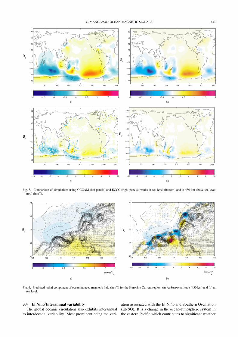
the surface velocity data from ECCO simulations as givenin Fig. 8. The mean surface layer velocity vectors (depthdown to 60 m) for the November 1997 (El Nino) and theNovember 1999 (La Nina) periods show a dramatic rever-sal in flow direction. The depth extent of these currents isgiven in a stacked velocity plot (left panel of Fig. 9) for arectangular area of latitude 0◦–5◦ and longitude 200◦–212◦.The influence of El Nino on the velocity seems to exist onlyin the upper 250 meters of the ocean. The velocities arewithin a range of ±0.2 m/s and have negligible magnitudefor depth >250 m.

We averaged the circulation velocity data from June 1997

to May 1998 to represent the flow during the El Nino pe-riod. In addition, we computed the annual mean velocityfor the year 1999 to represent the La Nina period. The pre-dicted magnetic fields for the El Nino and La Nina periodsare dominated by the gradients associated with ACC, with aweak amplitude range of ±0.2 nT. The difference of thesetwo predictions, although very weak, show an anomalytrending EW, as one would have expected from currentsreversal. However this is probably dominated by velocityfluctuations associated with some other phenomena (rightpanel of the Fig. 9). In any case, the variability in the mag-netic field has very low amplitude, as compared to seasonal

436 C. MANOJ et al.: OCEAN MAGNETIC SIGNALS

−0.1 −0.05 0 0.05 0.1 0.15 0.2−500

−400

−300

−200

−100

0

Dep

th

Velocity m/s

November 1997 (El Nino)

November 1999 (LaNina)

200 220 240 260 280

−15

−10

−5

0

5

10

15

−0.06 −0.04 −0.02 0 0.02

Fig. 9. Left panel: Stacked velocity (zonal) depth profiles for La Nina and El Nino periods (depth in m). Right panel: The difference of predictedmagnetic fields between El Nino and La Nina periods (in nT).

variation. The reasons for such small variation could be: 1)The El Nino affects only a thin surface layer in the ocean,and the surface current reversal fails to produce apprecia-ble changes in the depth integrated velocity, and 2) the lowstrength of the radial component of the Earth’s magneticfield at low geomagnetic latitudes.

4. Summary and ConclusionWe predicted the magnetic field generated by ocean cir-

culation using a global EM induction code based on the vol-ume integral equation approach and considering a realistic3D conductivity distribution for the Earth. The ocean circu-lation data were from two models viz. ECCO and OCCAMwith 1◦ × 1◦ resolution and 0.25◦ × 0.25◦ resolutions, re-spectively. Magnetic fields predicted by both models havean amplitude range of ±2 nT at satellite altitude. Thesefields are predominantly influenced by the ACC and West-ern Boundary current. At satellite altitude the ocean modelresolution does not have a strong influence on the patternand amplitude of the magnetic signals. At sea level, how-ever, the ECCO simulations have considerably less strengththan those using OCCAM. A reason could be the pres-ence of small scale circulation features such as ocean ed-dies in the OCCAM data. This is clearly visible along theKuroshio current region where the OCCAM data producean amplitude range of ±10 nT. Nevertheless, effects of in-dividual eddies are not evident when the magnetic fields areupwardly continued to Swarm altitude (430 km). Seasonaland interannual variations in the predicted magnetic fieldswere simulated by the data from the ECCO model. Thedifference between Summer and Winter data for the year2002 has an amplitude range of ±0.2 nT at satellite alti-tude. An interesting region is the Indian Ocean. The vari-ations in the magnetic field related to the surface currentreversal during the 1997–1998 El Nino event produced con-siderably smaller amplitude than expected, probably due toits proximity to the geomagnetic equator. The small am-plitude in the temporal magnetic variability seen in theseresults is in general agreement with previous studies (usingOPYC and ECCO ocean model data) by J. Oberhuber andR. Tyler which have been presented at international confer-

ences (Tyler et al., 1998; Tyler, 2002, 2003). Because thesethree different studies involved three rather different pa-rameterizations and numerical methods for calculating themagnetic fields from the flow there is now reasonable con-fidence that the small variability is not simply an artifact ofeither the numerical method or parameterizations.

Our simulations show a significant contribution of theocean circulation generated magnetic signals at sea andsatellite altitude. At sea level, the strong signals from theocean eddies indicate the need of using higher resolution(0.25◦ × 0.25◦ or less) ocean circulation data to model theeffects expected in ground based magnetometer data. Atsatellite altitude, the similar strength and global pattern ofthe magnetic signals predicted from two independent oceancirculation models also strengthens the case for being ableto identify non-tidal ocean magnetic signals in future satel-lite data. Presently, however, the separation of these signalsfrom the crustal magnetic fields in the satellite data maybe difficult. Maus et al. (2005) showed the importance ofcorrecting satellite data for tidal magnetic signals in crustalfield modelling. Considering the non trivial contribution ofthe magnetic field from the ocean circulation, we proposeto correct future crustal field anomaly maps by subtractingthe predicted signals of the steady ocean circulation. AsSwarm intends to bring out higher resolution crustal fieldanomaly map, this correction gains more importance. Withthe increasing precision in the modeling and measurementof geomagnetic fields, the identification of non-tidal oceanmagnetic signals from satellite data and their use to gain in-formation about global ocean water transport and their vari-ations, stands as a realistic possibility.

Acknowledgments. ECCO and OCCAM ocean models wereused to derive the ocean transport. ECCO is a contribution ofthe Consortium for Estimating the Circulation and Climate of theOcean (ECCO) funded by the National Oceanographic Partner-ship Program, USA. The Swarm end-to-end simulation studywas sponsored by the European Space Agency (ESA). One ofthe authors (CM) acknowledges the permission of the Director,NGRI, Hyderbadad, India to publish this paper. Comments fromRobert Tyler, Mike Purucker and Nils Olsen improved the originalmanuscript.

C. MANOJ et al.: OCEAN MAGNETIC SIGNALS 437

ReferencesChave, A., On the theory of electromagnetic induction in the earth by ocean

currents, J. Geophys. Res., 88, 3531–3542, 1983.Everett, M., S. Constable, and C. Constable, Effects of near-surface con-

ductance on global satellite induction responses, Geophys. J. Int., 153,277–286, 2003.

Faraday, M., Experimental researches in electricity (Bakerian lecture),Philos. Trans. R. Soc. London, 122, 163–177, 1832.

Flosadottir, A. H., J. C. Larsen, and J. T. Smith, Motional inductionin North Atlantic circulation models, J. Geophys. Res., 102, 10,353–10,372, 1997a.

Flosadottir, A. H., J. C. Larsen, and J. T. Smith, The relation of seafloorvoltages to ocean transports in North Atlantic circulation models: Modelresults and practical considerations for transport monitoring, J. PhysicalOceanography, 27, 1547–1565, 1997b.

Fofonoff, N. P., Physical properties of seawater: A new salinity scale andequation of state for seawater, J. Geophys. Res., 90, 3322–3342, 1985.

Junge, A., The telluric field in northern Germany induced by tidal motionin North Sea, Geophys. J. Int., 95, 523–533, 1988.

Kuvshinov, N. and N. Olsen, 3-D modelling of the magnetic fields dueto ocean tidal flow, in Earth Observation with CHAMP. Results fromThree Years in Orbit, edited by C. Reigber, H. Luhr, P. Schwintzer, andJ. Wickert, pp. 359–366, Springer Verlag, 2005.

Kuvshinov, A. V., D. B. Avdeev, O. V. Pankratov, S. A. Golyshev, andN. Olsen, Modelling electromagnetic fields in 3D spherical Earth usingfast integral equation approach, in 3D Electromagnetics, edited by M. S.Zhdanov, and P. E. Wannamaker, chap. 3, pp. 43–54, Elsevier, Holland,2002.

Kuvshinov, A. V., H. Utada, D. Avdeev, and T. Koyama, 3-D modelling andanalysis of Dst C-responses in the North Pacific Ocean region, revisited,Geophys. J. Int., 160, 505–526, 2005.

Larsen, J. C., Electric and magnetic fields induced by deep see tides,Geophys. J. R. Astr. Soc., 16, 47–70, 1968.

Larsen, J. C. and T. Sanford, Florida Current volume transport from volt-age measurements, Science, 227, 302–304, 1985.

Laske, G. and G. Masters, A global digital map of sediment thickness, EOSTrans. AGU, 78, F483, 1997.

Lilley, F., A. White, G. Heinson, and K. Procko, Seeking a seafloor mag-netic signal from the Antarctic Circumpolar Current, Geophys. J. Int.,157, 175–186, 2004a.

Lilley, F., A. Hitchman, P. R. Milligan, and T. Pedersen, Sea-surface obser-vations of the magnetic signals of ocean swells, Geophys. J. Int., 159,565–572, 2004b.

Marshall, J., A. Adcroft, C. Hill, Perelman, and C. Heisey, A finite-volume,incompressible Navier-Stokes model for studies of the ocean on parallelcomputers, J. Geophys. Res., 102, 5753–5766, 1997.

Maus, S. and A. Kuvshinov, Ocean tidal signals in observatoryand satellite magnetic measurements, Geophyc. Res. Lett, 31,

doi:10.1029/2004GC000, 634, 2004.Maus, S., M. Rother, K. Hemant, H. Luhr, A. Kuvshinov, and N. Olsen,

Earth’s crustal magnetic field determined to spherical harmonic degree90 from CHAMP satellite measurements, Geophys. J. Int., 164, 319–330, doi:10.1111/j.1365-246X.2005.02833.x, 2006.

Palshin, N., L. Vanyan, I. Yegorov, and K. Lebedev, Electric field inducedby the glodal ocean circulation, Physics Solid Earth, 35, 1028–1035,1999.

Pankratov, O., A. Kuvshinov, and D. Avdeev, High-performance three-dimensional electromagnetic modeling using modified Neumann series.Anisotropic case, J. Geomag. Geoelectr., 49, 1541–1547, 1997.

Sanford, T. B., Motionally induced electric and magnetic fields in the sea,J. Geophys. Res., 76, 3476–3492, 1971.

Schmucker, U., Electrical properties of the Earth’s interior, in Landolt-Bornstein, New-Series, 5/2b, pp. 370–397, Springer-Verlag, Berlin-Heidelberg, 1985.

Singer, B., Method for solution of Maxwell’s equations in non-uniformmedia, Geophys. J. Int., 120, 590–598, 1995.

Stephenson, D. and K. Bryan, Large-scale electric and magnetic fieldsgenerated by the oceans, J. Geophys. Res., 97, 15,467–15,480, 1992.

Tyler, R. H., Theoretical and Numerical Results on the Magnetic FieldsGenerated by Ocean Flow, EGS annual conference, 2002.

Tyler, R. H., Exploring and exploiting the magnetic fields generated byocean flow, Geophysical Research Abstracts, 5, 2003.

Tyler, R., L. A. Mysak, and J. Oberhuber, Electromagnetic fields generatedby a 3-D global ocean circulation, J. Geophys. Res., 102, 5531–5551,1997.

Tyler, R. H., T. B. Sanford, and J. M. Oberhuber, Magnetic Fields Gener-ated by Ocean Flow, AGU Fall Conference, 1998.

Tyler, R., J. Oberhuber, and T. Sanford, The potential for using ocean gen-erated electromagnetic field to remotely sense ocean variability, Phys.Chem. Earth (A), 24, 429–432, 1999.

Tyler, R., S. Maus, and H. Luhr, Satellite observations of magnetic fieldsdue to ocean tidal flow, Science, 299, 239–240, 2003.

Vivier, F., E. Maier-Reimer, and R. H. Tyler, Simulations of magnetic fieldsgenerated by the Antarctic Circumpolar Current at satellite altitude: Cangeomagnetic measurements be used to monitor the flow?, Geophys. Res.Lett., 31, doi:10.1029/2004GL019, 804, 2004.

Webb, D. J., B. A. de Cuevas, and A. C. Coward, The first main run ofthe OCCAM global ocean model, Internal Document 34, SouthamptonOceanography Centre, U.K., 1998.

Zhang, S.-L., GPBi-CG: generalized product-type methods based on Bi-CG for solving nonsymmetric linear systems, SIAM J. Sci. Comput., 18,537–551, 1997.

C. Manoj (e-mail: manoj@gfz-potsdam.de), A. Kuvshinov, S. Maus,and H. Luhr