Obtaining Predictive Distributions for Reserves Which ... · Variance Advancing the Science of Risk 1. Introduction There has been a lot of attention given to sto-chastic reserving

Obtaining Predictive Distributionsfor Reserves Which Incorporate

Expert Opinionby R. J. Verrall

ABSTRACT

This paper shows how expert opinion can be inserted intoa stochastic framework for loss reserving. The reservingmethods used are the chain-ladder and Bornhuet-ter-Ferguson, and the stochastic framework follows Eng-land and Verrall [8]. Although stochastic models have beenstudied, there are two main obstacles to their more frequentuse in practice: ease of implementation and adaptability touser needs. This paper attempts to address these obstaclesby utilizing Bayesian methods, and describing in some de-tail the implementation, using freely available software andprograms supplied in the Appendix.

KEYWORDS

Bayesian statistics, Bornhuetter-Ferguson, chain-ladder, claims reserving,expert opinion, risk

Variance Advancing the Science of Risk

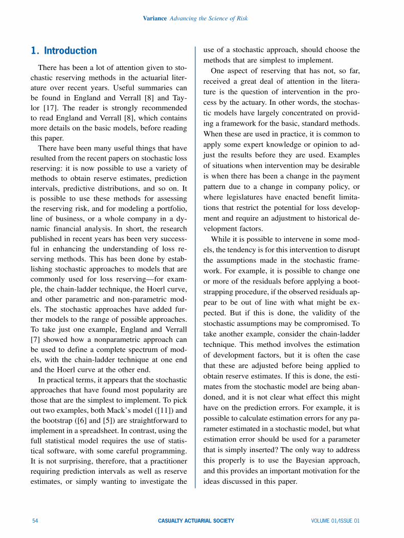
1. Introduction

There has been a lot of attention given to sto-chastic reserving methods in the actuarial liter-ature over recent years. Useful summaries canbe found in England and Verrall [8] and Tay-lor [17]. The reader is strongly recommendedto read England and Verrall [8], which containsmore details on the basic models, before readingthis paper.There have been many useful things that have

resulted from the recent papers on stochastic lossreserving: it is now possible to use a variety ofmethods to obtain reserve estimates, predictionintervals, predictive distributions, and so on. Itis possible to use these methods for assessingthe reserving risk, and for modeling a portfolio,line of business, or a whole company in a dy-namic financial analysis. In short, the researchpublished in recent years has been very success-ful in enhancing the understanding of loss re-serving methods. This has been done by estab-lishing stochastic approaches to models that arecommonly used for loss reserving–for exam-ple, the chain-ladder technique, the Hoerl curve,and other parametric and non-parametric mod-els. The stochastic approaches have added fur-ther models to the range of possible approaches.To take just one example, England and Verrall[7] showed how a nonparametric approach canbe used to define a complete spectrum of mod-els, with the chain-ladder technique at one endand the Hoerl curve at the other end.In practical terms, it appears that the stochastic

approaches that have found most popularity arethose that are the simplest to implement. To pickout two examples, both Mack’s model ([11]) andthe bootstrap ([6] and [5]) are straightforward toimplement in a spreadsheet. In contrast, using thefull statistical model requires the use of statis-tical software, with some careful programming.It is not surprising, therefore, that a practitionerrequiring prediction intervals as well as reserveestimates, or simply wanting to investigate the

use of a stochastic approach, should choose themethods that are simplest to implement.One aspect of reserving that has not, so far,

received a great deal of attention in the litera-ture is the question of intervention in the pro-cess by the actuary. In other words, the stochas-tic models have largely concentrated on provid-ing a framework for the basic, standard methods.When these are used in practice, it is common toapply some expert knowledge or opinion to ad-just the results before they are used. Examplesof situations when intervention may be desirableis when there has been a change in the paymentpattern due to a change in company policy, orwhere legislatures have enacted benefit limita-tions that restrict the potential for loss develop-ment and require an adjustment to historical de-velopment factors.While it is possible to intervene in some mod-

els, the tendency is for this intervention to disruptthe assumptions made in the stochastic frame-work. For example, it is possible to change oneor more of the residuals before applying a boot-strapping procedure, if the observed residuals ap-pear to be out of line with what might be ex-pected. But if this is done, the validity of thestochastic assumptions may be compromised. Totake another example, consider the chain-laddertechnique. This method involves the estimationof development factors, but it is often the casethat these are adjusted before being applied toobtain reserve estimates. If this is done, the esti-mates from the stochastic model are being aban-doned, and it is not clear what effect this mighthave on the prediction errors. For example, it ispossible to calculate estimation errors for any pa-rameter estimated in a stochastic model, but whatestimation error should be used for a parameterthat is simply inserted? The only way to addressthis properly is to use the Bayesian approach,and this provides an important motivation for theideas discussed in this paper.

54 CASUALTY ACTUARIAL SOCIETY VOLUME 01/ISSUE 01

Obtaining Predictive Distributions for Reserves Which Incorporate Expert Opinion

A second area where expert knowledge is ap-plied is when the Bornhuetter-Ferguson [1] tech-nique is used. This method uses the develop-ment factors from the chain-ladder technique, butit does not apply these to the latest cumulativelosses to estimate the outstanding losses. Instead,an estimate is first procured separately, usingbackground knowledge about the claims. This isthen used with the development factors to obtainreserve estimates. Although not originally for-mulated using a Bayesian philosophy, the Born-huetter-Ferguson technique is quite clearly suitedto this approach because of the basic idea ofwhat it is trying to do: incorporate expert opin-ion. Thus, we have a second important motiva-tion for considering the use of Bayesian reserv-ing methods. These are two very important ex-amples of reserving approaches commonly used,which are best modeled using Bayesian methods.Among previous papers to discuss Bayesian lossreserving, we would mention de Alba [4] andNtzoufras and Dellaportas [13].One important property of Bayesian methods

that makes them suitable for use with a stochas-tic reserving model is that they allow us to incor-porate expert knowledge in a natural way, over-coming any difficulties about the effect on theassumptions made. In this paper, we consider theuse of Bayesian models for loss reserving in or-der to incorporate expert opinion into the pre-diction of reserves. We concentrate on two areasas mentioned above: the Bornhuetter-Fergusontechnique and the insertion of prior knowledgeabout individual development factors in thechain-ladder technique. The possibility of includ-ing expert knowledge is an important propertyof Bayesian models, but there is another equallyimportant point: the ease with which they canbe implemented. This is due to modern devel-opments in Bayesian methodology based on so-called “Markov chain Monte Carlo” (MCMC)methods. It is difficult to emphasize enough theeffect these methods have had on Bayesian statis-

tics, but the books by Congdon ([3] and [2]) givesome idea of the scope of the applications forwhich they have been used. The crucial aspectas far as this paper is concerned is that they arebased on simulation, and therefore have somesimilarities with bootstrapping methods that, aswas mentioned above, have gained in popularityfor loss reserving.It is also important that easy-to-use software

is now available that allows us to implement theBayesian models for loss reserving. While it isstraightforward to define a Bayesian model, it isnot always so easy to find the required posteriordistributions for the parameters and predictivedistributions for future observations. However,this has been made much easier in recent years bythe development of MCMC methods, and by thesoftware package winBUGS [16]. This softwarepackage is freely available from http://www.mrc-bsu.cam.ac.uk/bugs, and the programs for car-rying out the Bayesian analysis for the modelsdescribed in this paper are contained in the Ap-pendix. Section 6.1 provides instructions ondownloading this software. An excellent refer-ence for actuarial applications of MCMC meth-ods using winBUGS is Scollnik [15].The basic idea behind MCMC methods is to

simulate the posterior distribution by breakingthe simulation process down into a number ofsimulations that are as easy to carry out as pos-sible. This overcomes a common problem withBayesian methods–that it can be difficult to de-rive the posterior distribution, which may inmany cases be multidimensional. Instead of try-ing to simulate all the parameters at once, MCMCmethods use the conditional distribution of eachparameter, given all the others. In this way, thesimulation is reduced to a univariate distribution,which is much easier to deal with. A Markovchain is formed because each parameter is con-sidered in turn, and it is a simulation-basedmethod: hence the term Markov chain MonteCarlo. For the readers for whom this is the first

VOLUME 01/ISSUE 01 CASUALTY ACTUARIAL SOCIETY 55


time they have encountered MCMC methods, itis suggested that they simply accept that they area neat way to get the posterior distributions forBayesian models and continue reading the paper.If they like the ideas and would like to find outmore, Scollnik [15] gives a much fuller accountthan is possible here, and the reader is advisedto spend time working through some simpler ex-amples with the help of the Scollnik paper.This paper is set out as follows. In Section 2,

we describe the notation and basic methods used,and in Section 3 we summarize the stochasticmodels used in the context of the chain-laddertechnique. Sections 4 and 5 describe the Bayesianmodels for incorporating prior information intothe reserving process. In Section 6 we describein some detail how to implement the Bayesianmodels so that the reader can investigate the useof these models, using the programs given in theAppendix. In Section 7 we state some conclu-sions.

2. Notation and basic methods

To begin with, we define the notation used inthis paper, and in doing so we briefly summarizethe chain-ladder technique and the Bornhuetter-Ferguson method.Although the methods can also be applied to

other shapes of data, in order that the notationshould not get too complicated we make the as-sumption that the data is in the shape of a trian-gle. Thus, without loss of generality, we assumethat the data consist of a triangle of incrementallosses:

C11 C12 ¢ ¢ ¢ C1n

C21 ¢ ¢ ¢ C2,n¡1...

Cn1

:

This can also be written as fCij : j = 1, : : : ,n¡i+1; i = 1, : : : ,ng, where n is the number of ac-cident years. Cij is used to denote incremental

losses, and Dij is used to denote the cumulativelosses, defined by:

Dij =jXk=1

Cik: (2.1)

One of the methods considered in this paper isthe chain-ladder technique, and the developmentfactors f¸j : j = 2, : : : ,ng. The usual estimates ofthe development factors from the standard chain-ladder technique are

ˆj =

Pn¡j+1i=1 DijPn¡j+1

i=1 Di,j¡1: (2.2)

Note that we only consider forecasting lossesup to the latest development year (n) so far ob-served, and no tail factors are applied. It wouldbe possible to extend this to allow a tail factor,using the same methods, but no specific model-ing is carried out in this paper of the shape ofthe run-off beyond the latest development year.Thus, we refer to cumulative losses up to de-velopment year n, Din =

Pnk=1Cik, as “ultimate

losses.” For the chain-ladder technique, the es-timate of outstanding losses is Di,n¡i+1( ˆ n¡i+2¢ ˆn¡i+3 : : : ˆ n¡ 1).The first case we consider is when these de-

velopment factor estimates are not used for allrows. In other words, we consider the more gen-eral case where there is a separate developmentfactor in each row, ¸i,j . The standard chain-laddermodel sets ¸i,j = ¸j , for i = 1,2, : : : ,n¡ j+1;j = 2,3, : : : ,n, but we consider allowing the moregeneral case where development factors canchange from row to row. Section 4 describesthe Bayesian approach to this, allowing expertknowledge to be used to set prior distributionsfor these parameters. In this way, we will be ableto intervene in the estimation of the developmentfactors, or else simply leave them for the standardchain-ladder model to estimate.In Section 5 we consider the Bornhuetter-

Ferguson method. This method uses the develop-ment factors from the chain-ladder technique, but



it incorporates knowledge about the “level” ofeach row by replacing the chain-ladder estimateof outstanding claims, Di,n¡i+1( ˆn¡i+2 ˆn¡i+3 : : :ˆn¡ 1) by Mi(1=(

ˆn¡i+2 ˆ n¡i+3 : : : ˆn))( ˆ n¡i+2

¢ ˆn¡i+3 : : : ˆn¡ 1). Here, Mi denotes a value forthe ultimate losses for accident year i that is ob-tained using expert knowledge about the losses(for example, taken from the premium calcula-tion). Thus, Mi(1=(

ˆn¡i+2 ˆn¡i+3 : : : ˆ n)) replaces

the latest cumulative losses for accident year i, towhich the usual chain-ladder parameters are ap-plied to obtain the estimate of outstanding losses.From this, it can be seen that the difference be-tween the Bornhuetter-Ferguson method and thechain-ladder technique is that the Bornhuetter-Ferguson technique uses an external estimate ofthe “level” of each row in the triangle, while thechain-ladder technique uses the data in that rowitself. The Bornhuetter-Ferguson method can beformulated using a Bayesian approach, with theinformation about the external estimates for eachrow being used to form the prior distributions, asin Section 5.This section has defined the notation used in

the paper, and outlined the basic reserving meth-ods that will be considered using stochastic ap-proaches. In order to do this, a brief introductionto the stochastic models is needed, and this isgiven in Section 3.

3. Stochastic models for thechain-ladder technique

This section gives a brief summary of stochas-tic models that are related to the chain-laddertechnique. A much fuller account may be foundin England and Verrall [8], and in that paper’sreferences and discussion. We consider the chain-ladder technique and note that it is possible to ap-ply Bayesian methods in a similar way to othermodels.There are a number of different approaches

that can be taken to the chain-ladder technique,with various positivity constraints, all of which

give the same reserve estimates as the chain-ladder technique. The connections between thechain-ladder technique and various stochasticmodels have been explored in a number of pre-vious papers. For example, Mack [11] takes anon-parametric approach and specifies only thefirst two moments for the cumulative losses. InMack’s model the conditional mean and varianceof Dij jDi,j¡1,¸j ,¾2j are ¸jDi,j¡1 and ¾2j Di,j¡1,respectively. Estimates of all the parameters arederived, and the properties of the model are ex-amined. As was stated in the introduction, oneof the advantages of this approach is that the pa-rameter estimates and prediction errors can beobtained using a spreadsheet, without having re-course to a statistical package or any complexprogramming. The consequence of not specify-ing a distribution for the data is that there is nopredictive distribution. Also, there are separateparameters in the variance that must also be esti-mated, separately from the estimation of the de-velopment factors.As a separate stream of research, generalized

linear models have also been considered. Ren-shaw and Verrall [14] used an approach basedon generalized linear models [12] and examinedthe over-dispersed Poisson model for incremen-tal losses:

Cij j c,®,¯,'» independent over-dispersed

Poisson, with mean, mij , where log(mij) =c+®i+¯j , and ®1 = ¯1 = 0:

The term “over-dispersed” requires someexplanation. It is used here in connection withthe Poisson distribution, and it means that if X »Poisson(¹), then Y = 'X follows the over-dis-persed Poisson distribution with E(Y) = '¹ andV(Y) = '2E(X) = '2¹. ' is usually greater than1–hence the term “over-dispersed”–but this isnot a necessity. It can also be used for other dis-tributions, and we make use of it for the negativebinomial distribution. As with the Poisson distri-bution, the over-dispersed negative binomial dis-



tribution is defined such that if X » negative bi-nomial then Y = 'X follows the over-dispersednegative binomial distribution. Furthermore, aquasi-likelihood approach is taken so that theloss data are not restricted to the positive inte-gers.It can be seen that this formulation has some

similarities with the model of Kremer [9], but ithas a number of advantages. It does not necessar-ily break down if there are negative incrementalloss values, it gives the same reserve estimates asthe chain-ladder technique, and it has been foundto be more stable than the log-normal model ofKremer. For these reasons, we concentrate on itin this paper. There are a number of ways ofwriting this model, which are useful in differentcontexts (note that the reserve estimates are un-affected by the way the model is written). In astrict sense, the formulation requires that the dataare positive–otherwise it is more difficult to jus-tify and interpret the inferences made from thedata. However, in a purely practical context, it isuseful to note that the estimation does not breakdown in the presence of some negative values.Another way of writing the over-dispersed

Poisson model for the chain-ladder technique isas follows:

Cij j x,y,'» independent over-dispersedPoisson, with mean xiyj , and

Xn

k=1yk = 1:

Here x= fx1,x2, : : : ,xng and y = fy1,y2, : : : ,yngare parameter vectors relating to the rows (acci-dent years) and columns (development years), re-spectively, of the run-off triangle. The parameterxi = E[Din], and so represents expected ultimatecumulative losses (up to the latest developmentyear so far observed, n) for the ith accident year.The column parameters, yj , can be interpreted asthe proportions of ultimate losses that emerge ineach development year.Although the over-dispersed Poisson models

give the same reserve estimates as the chain-ladder technique (as long as the row and col-

umn sums of incremental claims are positive),the connection with the chain-ladder technique isnot immediately apparent from this formulationof the model. For this reason, the negative bino-mial model was developed by Verrall [20], build-ing on the over-dispersed Poisson model. Verrallshowed that the same predictive distribution canbe obtained from a negative binomial model (alsowith the inclusion of an over-dispersion param-eter). In this recursive approach, the incrementalclaims have an over-dispersed negative binomialdistribution, with mean and variance

(¸j ¡ 1)Di,j¡1 and '¸j(¸j ¡ 1)Di,j¡1,respectively.

Again, the reserve estimates are the same asthe chain-ladder technique, and the same posi-tivity constraints apply as for the over-dispersedPoisson model. It is clear from this that the col-umn sums must be positive, since a negative sumwould result in a development factor less than 1(¸j < 1), causing the variance to be negative. Itis important to note that exactly the same pre-dictive distribution can be obtained from eitherthe Poisson or negative binomial models. Verrall[20] also argued that the model could be speci-fied either for incremental or cumulative losses,with no difference in the results. The negative bi-nomial model has the advantage that the form ofthe mean is exactly the same as that which nat-urally arises from the chain-ladder technique. Infact, by adding the previous cumulative losses,an equivalent model for Dij jDi,j¡1,¸j ,' has anover-dispersed negative binomial distribution,with mean and variance

¸jDi,j¡1 and '¸j(¸j ¡ 1)Di,j¡1, respectively.

Here the connection with the chain-laddertechnique is immediately apparent because of theformat of the mean.Another model, which is not considered fur-

ther in this paper, is closely connected withMack’s model, and deals with the problem of



negative incremental claims. This model replacesthe negative binomial by a normal distribution,whose mean is unchanged, but whose varianceis altered to accommodate the case when ¸j < 1.Preserving as much of ¸j(¸j ¡ 1)Di,j¡1 as pos-sible, the variance is still proportional to Di,j¡1,with the constant of proportionality dependingon j, but a normal approximation is used forthe distribution of incremental claims. Thus, Cij jDi,j¡1,¸j ,'j is approximately normally distribut-ed, with mean and variance

Di,j¡1(¸j ¡ 1) and 'jDi,j¡1, respectively,

or Dij jDi,j¡1,¸j ,'j is approximately normallydistributed, with mean and variance

¸jDi,j¡1 and 'jDi,j¡1, respectively.

As for Mack’s model, there is now another setof parameters in the variance that needs to beestimated.For each of these models, the mean square er-

ror of prediction can be obtained, allowing theconstruction of prediction intervals, for exam-ple. Loss reserving is a predictive process: giventhe data, we try to predict future loss emergence.These models apply to all the data, both observedand future observations. The estimation is basedon the observed data, and we require predictivedistributions for the future observation.We use the expected value of the distribution

of future losses as the prediction. When con-sidering variability, attention is focused on theroot mean squared error of prediction (RMSEP),also known as the prediction error. To explainwhat this is, we consider, for simplicity, a randomvariable, y, and a predicted value y. The meansquared error of prediction (MSEP) is the ex-pected square difference between the actual out-come and the predicted value, E[(y¡ y)2], andcan be written as follows:

E[(y¡ y)2] = E[((y¡E[y])¡ (y¡E[y]))2]:(3.1)

In order to obtain an estimate of this, it is nec-essary to plug in y instead of y in the final ex-pectation. Then the MSEP can be expanded asfollows:

E[(y¡ y)2]¼ E[(y¡E[y])2]¡ 2E[(y¡E[y])(y¡E[y])]+E[(y¡E[y])2]: (3.2)

Assuming future observations are independent ofpast observations, the middle term is zero, and

E[(y¡ y)2]¼ E[(y¡E[y])2]+E[(y¡E[y])2]:(3.3)

In words, this is

prediction variance= process variance+ estimation variance.

It is important to understand the difference be-tween the prediction error and the standard error.Strictly, the standard error is the square root ofthe estimation variance. The prediction error isconcerned with the variability of a forecast, tak-ing account of uncertainty in parameter estima-tion and also of the inherent variability in thedata being forecast. Further details of this can befound in England and Verrall [8].Using non-Bayesian methods, these two com-

ponents–the process variance and the estima-tion variance–are estimated separately, and Sec-tion 7 of England and Verrall [8] goes into detailabout this. The direct calculation of these quan-tities can be a tricky process, and this is one ofthe reasons for the popularity of the bootstrap.The bootstrap uses a fairly simple simulation ap-proach to obtain simulated estimates of the pre-diction variance in a spreadsheet. Fortunately, thesame advantages apply to the Bayesian methods:the full predictive distribution can be found us-ing simulation methods, and the RMSEP can beobtained directly by calculating its standard de-viation. In addition, it is preferable to have thefull predictive distribution, rather than just the



first two moments, which is another advantageof Bayesian methods.The purpose of this paper is to show how ex-

pert opinion, from sources other than the spe-cific data set under consideration, can be incor-porated into the predictive distributions of the re-serves. We use the approach of generalized lin-ear models outlined in this section, concentratingon the over-dispersed Poisson and negative bino-mial models. We begin with considering how it ispossible to intervene in the development factorsfor the chain-ladder technique in Section 4, andthen consider the Bornhuetter-Ferguson methodin Section 5.

4. Incorporating expert opinionabout the development factors

In this section, the approach of Verrall andEngland [21] is used to show how to specify aBayesian model that allows the practitioner to in-tervene in the estimation of the development fac-tors for the chain-ladder technique. There are anumber of ways in which this could be used, andwe describe some possibilities in this section. Itis expected that a practitioner would be able toextend these to cover situations that, although notspecifically covered here, would also be useful.The cases considered here are the intervention ina development factor in a particular row, and thechoice of how many years of data to use in theestimation. The reasons for intervening in theseways could be that there is information that thesettlement pattern has changed, making it inap-propriate to use the same development factor foreach row.For the first case, what may happen in prac-

tice is that a development factor in a particularrow is simply changed. Thus, although the samedevelopment parameters (and hence run-off pat-tern) are usually applied for all accident years, ifthere is some exogenous information that indi-cates that this is not appropriate, the practitioner

may decide to apply a different development fac-tor (or set of factors) in some, or all, rows.In the second case, it is common to look at, say,

five-year volume weighted averages in calculat-ing the development factors, rather than using allthe available data in the triangle. The Bayesianmethods make this particularly easy to do andare flexible enough to allow many possibilities.We use the negative binomial model described

in Section 3, with different development factorsin each row. This is the model for the data, andwe then specify prior distributions for the devel-opment factors. In this way, we can choose priordistributions that reproduce the chain-ladder re-sults, or we can intervene and use prior distribu-tions based on external knowledge. The modelfor incremental claims, Cij jDi,j¡1,¸i,j ,', is anover-dispersed negative binomial distribution,with mean and variance

(¸i,j ¡ 1)Di,j¡1 and '¸i,j(¸i,j ¡ 1)Di,j¡1, respectively.

We next need to define prior distributions forthe development factors, ¸i,j . It is possible to setsome of these equal to each other (within eachcolumn) in order to revert to the standard chain-ladder model. This is done by setting

¸i,j = ¸j for i = 1,2, : : : ,n¡ j+1;j = 2,3, : : : ,n

and defining vague prior distributions for ¸j(j = 2,3, : : : ,n). This was the approach taken inSection 8.4 of England and Verrall [8] and isvery similar to that taken by de Alba [4]. Thiscan provide a very straightforward method to ob-tain prediction errors and predictive distributionsfor the chain-ladder technique.However, we really want to move away from

the basic chain-ladder technique, and constructBayesian prior distributions that encompass theexpert opinion about the development parame-ters. Suppose, for example, that we have a 10£10 triangle. We consider the two possibilities forincorporating expert knowledge described above.



To illustrate the first case, suppose that thereis information that implies that the second de-velopment factor (from Column 2 to Column 3)should be given the value 1.5, for rows 8, 9, and10, and that there is no indication that the otherparameters should be treated differently from thestandard chain-ladder technique. An appropriateway to treat this would be to specify

¸i,j = ¸j for i = 1,2, : : : ,n¡ j+1;j = 2,4,5, : : : ,n

¸i,3 = ¸3 for i = 1,2, : : : ,7

¸8,3 = ¸9,3 = ¸10,3:

The means and variances of the prior distribu-tions of the parameters are chosen to reflect theexpert opinion:¸8,3 has a prior distribution with mean 1.5 and

varianceW, whereW is set to reflect the strengthof the prior information.¸j have prior distributions with large variances.For the second case, we divide the data into

two parts using the prior distributions. To do this,we set

¸i,j = ¸j for i= n¡ j¡ 3,n¡ j¡2,n¡ j¡ 1,n¡ j,n¡ j+1

¸i,j = ¸¤j for i= 1,2, : : : ,n¡ j¡4

and give both ¸j and ¸¤j prior distributions with

large variances so that they are estimated fromthe data. Adjustments to the specification aremade in the later development years, where thereare less than five rows. For these columns thereis just one development parameter, ¸j .The specific form of the prior distribution

(gamma, log-normal, etc.) is usually chosen sothat the numerical procedures in winBUGS workas well as possible.These models are used as illustrations of

the possibilities for incorporating expert knowl-edge about the development pattern, but it is (ofcourse) possible to specify many other prior dis-tributions. In the Appendix, the winBUGS codeis supplied, which can be cut and pasted directly

Table 1. Parameters, mean and variance of a gammadistribution

®i ¯i Mi Mi=¯i

10000 10 1000 1001000 1 1000 1000100 0.1 1000 10000

in order to examine these methods. Section 6contains a number of examples, including theones described in this section.

5. A Bayesian model for theBornhuetter-Ferguson method

In this section, we show how the Bornhuetter-Ferguson method can be considered in a Bayes-ian context, using the approach of Verrall [19].For further background on the Bornhuetter-Ferguson method, see Mack [10].In Section 3, the over-dispersed Poisson model

was defined as follows.

Cij j x,y,'» independent over-dispersedPoisson, with mean xiyj , and

Xn

k=1yk = 1:

In the Bayesian context, we also require priordistributions for the parameters. The Bornhuet-ter-Ferguson method assumes that there is ex-pert opinion about the level of each row, and wetherefore concentrate first on the specification ofprior distributions for these. The most convenientform to use is gamma distributions:

xi j ®i,¯i » independent ¡ (®i,¯i): (5.1)

There is a wide range of possible choices forthe parameters of these prior distributions, ®i and¯i. It is easiest to consider the mean and varianceof the gamma distribution, ®i=¯i and ®i=¯

2i , re-

spectively. These can be written as Mi and Mi=¯i,from which it can be seen that, for a given choiceofMi, the variance can be altered by changing thevalue of ¯i. To consider a simple example, sup-pose it has been decided that Mi = 1000. Table 1shows how the value of ¯i affects the variance ofthe prior distribution, while Mi is kept constant.



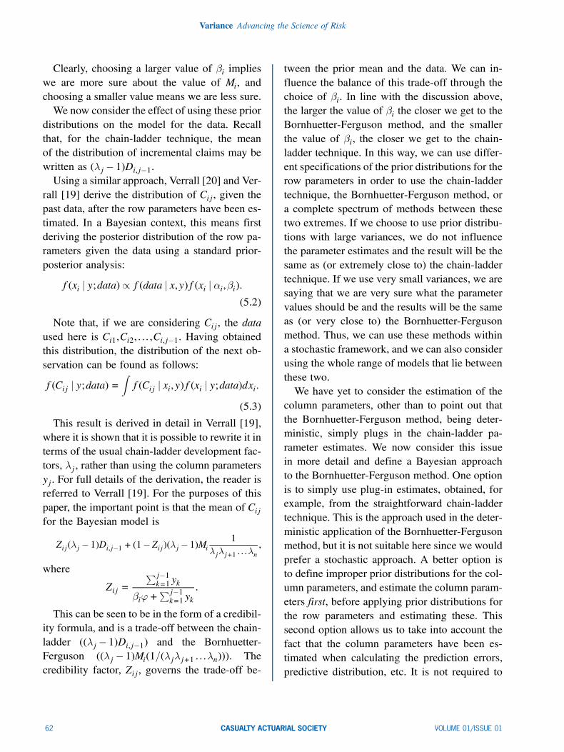
Clearly, choosing a larger value of ¯i implieswe are more sure about the value of Mi, andchoosing a smaller value means we are less sure.We now consider the effect of using these prior

distributions on the model for the data. Recallthat, for the chain-ladder technique, the meanof the distribution of incremental claims may bewritten as (¸j ¡ 1)Di,j¡1.Using a similar approach, Verrall [20] and Ver-

rall [19] derive the distribution of Cij , given thepast data, after the row parameters have been es-timated. In a Bayesian context, this means firstderiving the posterior distribution of the row pa-rameters given the data using a standard prior-posterior analysis:

f(xi j y;data)/ f(data j x,y)f(xi j ®i,¯i):(5.2)

Note that, if we are considering Cij , the dataused here is Ci1,Ci2, : : : ,Ci,j¡1. Having obtainedthis distribution, the distribution of the next ob-servation can be found as follows:

f(Cij j y;data) =Zf(Cij j xi,y)f(xi j y;data)dxi:

(5.3)

This result is derived in detail in Verrall [19],where it is shown that it is possible to rewrite it interms of the usual chain-ladder development fac-tors, ¸j , rather than using the column parametersyj . For full details of the derivation, the reader isreferred to Verrall [19]. For the purposes of thispaper, the important point is that the mean of Cijfor the Bayesian model is

Zij(¸j ¡ 1)Di,j¡1 + (1¡Zij)(¸j ¡ 1)Mi1

¸j¸j+1 : : :¸n,

where

Zij =Pj¡1k=1 yk

¯i'+Pj¡1k=1 yk

:

This can be seen to be in the form of a credibil-ity formula, and is a trade-off between the chain-ladder ((¸j ¡ 1)Di,j¡1) and the Bornhuetter-Ferguson ((¸j ¡ 1)Mi(1=(¸j¸j+1 : : :¸n))). Thecredibility factor, Zij , governs the trade-off be-

tween the prior mean and the data. We can in-fluence the balance of this trade-off through thechoice of ¯i. In line with the discussion above,the larger the value of ¯i the closer we get to theBornhuetter-Ferguson method, and the smallerthe value of ¯i, the closer we get to the chain-ladder technique. In this way, we can use differ-ent specifications of the prior distributions for therow parameters in order to use the chain-laddertechnique, the Bornhuetter-Ferguson method, ora complete spectrum of methods between thesetwo extremes. If we choose to use prior distribu-tions with large variances, we do not influencethe parameter estimates and the result will be thesame as (or extremely close to) the chain-laddertechnique. If we use very small variances, we aresaying that we are very sure what the parametervalues should be and the results will be the sameas (or very close to) the Bornhuetter-Fergusonmethod. Thus, we can use these methods withina stochastic framework, and we can also considerusing the whole range of models that lie betweenthese two.We have yet to consider the estimation of the

column parameters, other than to point out thatthe Bornhuetter-Ferguson method, being deter-ministic, simply plugs in the chain-ladder pa-rameter estimates. We now consider this issuein more detail and define a Bayesian approachto the Bornhuetter-Ferguson method. One optionis to simply use plug-in estimates, obtained, forexample, from the straightforward chain-laddertechnique. This is the approach used in the deter-ministic application of the Bornhuetter-Fergusonmethod, but it is not suitable here since we wouldprefer a stochastic approach. A better option isto define improper prior distributions for the col-umn parameters, and estimate the column param-eters first, before applying prior distributions forthe row parameters and estimating these. Thissecond option allows us to take into account thefact that the column parameters have been es-timated when calculating the prediction errors,predictive distribution, etc. It is not required to



include any information about the column pa-rameters, and hence we use improper gamma dis-tributions for the column parameters, and derivethe posterior distributions of these using a stan-dard Bayesian prior-posterior analysis. The re-sult of this is a distribution that looks similar tothe negative binomial model for the chain-laddertechnique, but which is recursive in i insteadof j:

Cij j C1,j ,C2,j , : : : ,Ci¡1,j ,x,'» over-dispersednegative binomial, with mean (°i¡ 1)

Pi¡1m=1Cm,j :

Comparing this to the mean of the chain-laddermodel, (¸j ¡ 1)Di,j¡1 = (¸j ¡ 1)

Pj¡1m=1Ci,m, it can

be seen that they are identical in form, with therecursion either being across the rows or downthe columns.In the context of the Bornhuetter-Ferguson

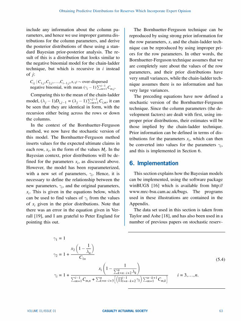
method, we now have the stochastic version ofthis model. The Bornhuetter-Ferguson methodinserts values for the expected ultimate claims ineach row, xi, in the form of the values Mi. In theBayesian context, prior distributions will be de-fined for the parameters xi, as discussed above.However, the model has been reparameterized,with a new set of parameters, °i. Hence, it isnecessary to define the relationship between thenew parameters, °i, and the original parameters,xi. This is given in the equations below, whichcan be used to find values of °i from the valuesof xi given in the prior distributions. Note thatthere was an error in the equation given in Ver-rall [19], and I am grateful to Peter England forpointing this out.

°1 = 1

°2 = 1+x2

µ1¡ 1

¸n

¶C1n

°i = 1+

xi

Ã1¡ 1Pn

k=n¡i+2¸k

!Pi¡1m=1Cm,n+

Pnk=n¡i+3

h³Qi¡1l=n¡k+2 °l

´Pn¡k+1m=1 Cm,k

i i = 3, : : : ,n:

(5.4)

The Bornhuetter-Ferguson technique can bereproduced by using strong prior information forthe row parameters, x, and the chain-ladder tech-nique can be reproduced by using improper pri-ors for the row parameters. In other words, theBornhuetter-Ferguson technique assumes that weare completely sure about the values of the rowparameters, and their prior distributions havevery small variances, while the chain-ladder tech-nique assumes there is no information and hasvery large variances.The preceding equations have now defined a

stochastic version of the Bornhuetter-Fergusontechnique. Since the column parameters (the de-velopment factors) are dealt with first, using im-proper prior distributions, their estimates will bethose implied by the chain-ladder technique.Prior information can be defined in terms of dis-tributions for the parameters xi, which can thenbe converted into values for the parameters °i,and this is implemented in Section 6.

6. Implementation

This section explains how the Bayesian modelscan be implemented, using the software packagewinBUGS [16] which is available from http://www.mrc-bsu.cam.ac.uk/bugs. The programsused in these illustrations are contained in theAppendix.The data set used in this section is taken from

Taylor and Ashe [18], and has also been used in anumber of previous papers on stochastic reserv-



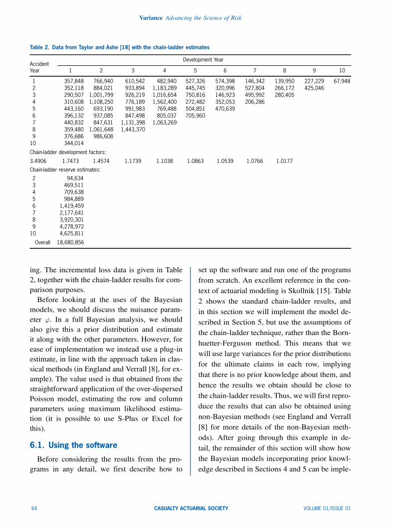
Table 2. Data from Taylor and Ashe [18] with the chain-ladder estimates

Development YearAccidentYear 1 2 3 4 5 6 7 8 9 10

1 357,848 766,940 610,542 482,940 527,326 574,398 146,342 139,950 227,229 67,9482 352,118 884,021 933,894 1,183,289 445,745 320,996 527,804 266,172 425,0463 290,507 1,001,799 926,219 1,016,654 750,816 146,923 495,992 280,4054 310,608 1,108,250 776,189 1,562,400 272,482 352,053 206,2865 443,160 693,190 991,983 769,488 504,851 470,6396 396,132 937,085 847,498 805,037 705,9607 440,832 847,631 1,131,398 1,063,2698 359,480 1,061,648 1,443,3709 376,686 986,608

10 344,014

Chain-ladder development factors:

3.4906 1.7473 1.4574 1.1739 1.1038 1.0863 1.0539 1.0766 1.0177

Chain-ladder reserve estimates:

2 94,6343 469,5114 709,6385 984,8896 1,419,4597 2,177,6418 3,920,3019 4,278,972

10 4,625,811

Overall 18,680,856

ing. The incremental loss data is given in Table2, together with the chain-ladder results for com-parison purposes.Before looking at the uses of the Bayesian

models, we should discuss the nuisance param-eter '. In a full Bayesian analysis, we shouldalso give this a prior distribution and estimateit along with the other parameters. However, forease of implementation we instead use a plug-inestimate, in line with the approach taken in clas-sical methods (in England and Verrall [8], for ex-ample). The value used is that obtained from thestraightforward application of the over-dispersedPoisson model, estimating the row and columnparameters using maximum likelihood estima-tion (it is possible to use S-Plus or Excel forthis).

6.1. Using the software

Before considering the results from the pro-grams in any detail, we first describe how to

set up the software and run one of the programsfrom scratch. An excellent reference in the con-text of actuarial modeling is Skollnik [15]. Table2 shows the standard chain-ladder results, andin this section we will implement the model de-scribed in Section 5, but use the assumptions ofthe chain-ladder technique, rather than the Born-huetter-Ferguson method. This means that wewill use large variances for the prior distributionsfor the ultimate claims in each row, implyingthat there is no prior knowledge about them, andhence the results we obtain should be close tothe chain-ladder results. Thus, we will first repro-duce the results that can also be obtained usingnon-Bayesian methods (see England and Verrall[8] for more details of the non-Bayesian meth-ods). After going through this example in de-tail, the remainder of this section will show howthe Bayesian models incorporating prior knowl-edge described in Sections 4 and 5 can be imple-



mented, and illustrate the effect that the choiceof prior distributions can have.The steps necessary for implementing the

chain-ladder technique in winBUGS are listedbelow.

1. Go to the web site, download the latest ver-sion of the software and install.

2. Go back to the web site and register, andyou will be sent a copy of the key to unlockthe software. Follow the instructions in theemail for unlocking the software.

3. Once you have a fully functioning versionof winBUGS, you can run the programs inthe Appendix. Open winBUGS and click on“File” in the top toolbar, and then “New”in the pop-down list. This will open a newwindow.

4. Copy the program in (i) of the Appendix,including the word “model” at the top and allthe data at the bottom, right down to wherethe next subsection begins at (ii). The lastline is 0,0,0,0,0,0,0,0,0)). Paste all of this intothe new window in winBUGS.

5. In winBUGS, select “Model” in the toolbarat the top and “Specification” in the pop-down list. This opens a new window called“Specification Tool.”

6. Highlight the word “model” at the top of theprogram, and then click “check model” inthe Specification Tool window. If all is well,it will say “model is syntactically correct” inthe bottom left corner.

7. Now move down in the window containingthe program until you get to #DATA. High-light the word “list” immediately below that,and click “load data” in the SpecificationTool window. It should say “data loaded” inthe bottom left corner.

8. Click “compile” in the Specification Toolwindow. After a few seconds, it should say“model compiled” in the bottom left corner.

9. Now move down in the window contain-ing the program until you get to #INITIALVALUES. Highlight the word “list” imme-diately below that, and click “load inits” inthe Specification Tool window. It should say“model is initialised” in the bottom left cor-ner.

10. Select “Model” in the toolbar at the top and“Update” in the pop-down list. This opensa new window called “Update Tool.” Thenumber of iterations in the simulation pro-cess can be changed in this window bychanging the figure next to “updates.” Just atthe moment, 1,000 is sufficient, so click on“update.” This runs 1,000 simulations with-out storing the results. This may take a fewminutes: don’t be concerned if nothing ap-pears to be happening! When it is complete,a message appears in the bottom left cornersaying how long the updates took (for mylaptop it was 221 seconds).

11. Select “Inference” in the toolbar at the topand “Samples” in the pop-down list. Thisopens a new window called “Sample Moni-tor Tool.” We want to look at the row totalsand overall total, which have been definedas a vector R and Total in the program. Inthe Sample Monitor Tool window, click inthe box to the right of the word “node” andtype R. Then click on “set.” Repeat for Total,noting that it is case sensitive.

12. Return to the Update Tool Window and clickon Update to perform 1,000 simulations.This should be quicker (6 seconds for mylaptop). This time the values of R and Totalwill be stored.

13. Return to the Sample Monitor Tool window,type * in the box to the right of the word“node,” and click “stats.” This will give anew window with something like the resultsbelow. This completes the steps necessaryfor fitting the Bayesian model.



Table 3. Results

Node Mean sd MC Error 2.5% Median 97.5% Start Sample

R[2] 92750.0 110600.0 2963.0 779.2 56320.0 412800.0 1001 1000R[3] 473900.0 223100.0 6424.0 1.52E+5 4.4E+5 1.011E+6 1001 1000R[4] 7.05E+5 2.58E+5 9085.0 307600.0 674500.0 1.288E+6 1001 1000R[5] 985800.0 304600.0 8127.0 467600.0 960600.0 1.667E+6 1001 1000R[6] 1.417E+6 378300.0 13430.0 768500.0 1.399E+6 2.217E+6 1001 1000R[7] 2.174E+6 5.19E+5 16850.0 1.271E+6 2.132E+6 3.233E+6 1001 1000R[8] 3.925E+6 776900.0 28100.0 2.585E+6 3.885E+6 5.555E+6 1001 1000R[9] 4.284E+6 1.066E+6 36840.0 2.464E+6 4.207E+6 6.731E+6 1001 1000R[10] 4.641E+6 2.002E+6 61630.0 1.73E+6 4.407E+6 9.345E+6 1001 1000

Total 1.87E+7 3.056E+6 101600.0 1.314E+7 1.861E+7 2.554E+7 1001 1000

The columns of Table 3 headed “mean” and“sd” give the predicted reserves and predictionerrors, and these values can be compared withthe chain-ladder results in Table 2. Since this isa simulation process, the results will depend onthe prior distributions, the initial values, and thenumber of iterations carried out. The prior dis-tributions in the program had reasonably largevariances, so the results should be close to thechain-ladder results. More simulations should beused in steps 10 and 12 (we use 10,000 in the il-lustrations below), and the prior variances couldbe increased. Using this number of simulationsgives the results shown in Table 4.The results certainly confirm that we can re-

produce the chain-ladder results, and producethe prediction errors. It is also possible toobtain other information about the model fromwinBUGS. For example, it is possible to pro-duce full predictive distributions, using “density”in the Sample Monitor Tool window.We have now described one implementation of

a Bayesian model using winBUGS. In the rest ofthis section, we consider the Bayesian models de-scribed in Sections 4 and 5 in order to considerhow expert opinion can be incorporated into thepredictive distribution of reserves. In each case,the programs are available in the Appendix, andthe results can be reproduced using steps 3 to 13,above. It should be noted that this is a simulation-based program, so the results obtained may not

Table 4. Chain-ladder results. the prediction error is equal tothe Bayesian standard deviation

Chain- Bayesian PredictionLadder Bayesian Standard ErrorReserve Mean Deviation (%)

Year 2 94,634 94,440 111,100 118%Year 3 469,511 471,400 219,400 47%Year 4 709,638 716,300 263,600 37%Year 5 984,889 991,600 308,100 31%Year 6 1,419,459 1,424,000 374,700 26%Year 7 2,177,641 2,186,000 497,200 23%Year 8 3,920,301 3,935,000 791,000 20%Year 9 4,278,972 4,315,000 1,068,000 25%Year 10 4,625,811 4,671,000 2,013,000 43%

Overall 18,680,856 18,800,000 2,975,000 16%

exactly match the results given below. However,there should be no significant differences, withthe differences that there are being due to simu-lation error.

6.2. Intervention in the chain-laddertechnique

We now consider using a prior distribution tointervene in some of the parameters of the chain-ladder model, instead of using prior distributionswith large variances that just reproduce the chain-ladder estimates. The implementation is set upin Section (ii) of the Appendix, and the programcan be cut and pasted into winBUGS and runfollowing steps 3 onwards, above.We consider two cases, as discussed in Sec-

tion 4. For the first case, we assume that there isinformation that implies that the second develop-



Table 5. Individual development factors

Development YearAccidentYear 2 3 4 5 6 7 8 9 10

1 3.143 1.543 1.278 1.238 1.209 1.044 1.04 1.063 1.0182 3.511 1.755 1.545 1.133 1.084 1.128 1.057 1.0863 4.448 1.717 1.458 1.232 1.037 1.12 1.0614 4.568 1.547 1.712 1.073 1.087 1.0475 2.564 1.873 1.362 1.174 1.1386 3.366 1.636 1.369 1.2367 2.923 1.878 1.4398 3.953 2.0169 3.619

ment factor (from Column 2 to Column 3) shouldbe given the value 1.5 for rows 7, 8, 9, and 10,and that there is no indication that the other pa-rameters should be treated differently from thestandard chain-ladder technique. In order to im-plement this, the parameter for the second de-velopment factor for rows 7—10 is given a priordistribution with mean 1.5. We then look at twodifferent choices for the prior variance for thisparameter. Using a large variance means that theparameter is estimated separately from the otherrows, but using the data without letting the priormean influence it too greatly. We then use a stan-dard deviation of 0.1 for the prior distribution, sothat the prior mean has a greater influence.We consider first the estimate of the second

development factor. The chain ladder estimate is1.7473 and the individual development factorsfor the triangle are shown in Table 5. The rowsfor the second development factor that are mod-eled separately are shown in italics. The estimateusing the Bayesian models is 1.68 for rows 1—6.When a large variance is used for the prior distri-bution of the development factor for rows 7—10,the estimate using the Bayesian model is 1.971.With the smaller variance for this prior distribu-tion, the estimate is 1.673, and has been drawndown towards the prior mean of 1.5. This clearlyshows how the prior distributions can be used toinfluence the parameter estimates.The effect on the reserve estimates is shown in

Table 6, which compares the reserves and predic-

tion errors for the two cases outlined above withthe results for the chain-ladder model (whichcould be produced using the program in Section6.1 on this set of data). The chain-ladder figuresare slightly different from those given in Table 4because this is a simulation method.It is interesting to note that, in this case, the

intervention has not had a marked effect on theprediction errors (in percentage terms). However,the prediction errors themselves have changedconsiderably, and this indicates that it is impor-tant to think of the prediction error as a percent-age of the prediction. Other prior distributionscould have a greater effect on the percentage pre-diction error.The second case we consider is when we use

only the most recent data for the estimation ofeach development factor. For the last three devel-opment factors, all the data is used because thereis no more than three years for each. For the otherdevelopment factors, only the three most recentyears are used. The estimates of the developmentfactors are shown in Table 7. The estimates ofthe first development factor are not affected bythe change in the model (the small differencescould be due to simulation error or the changeselsewhere). For the other development factors,the estimates can be seen to be affected by themodel assumptions.The effect of using only the latest three years

in the estimation of the development factors in



Table 6. Reserves and prediction errors for the chain-ladder and Bayesian models

Chain-Ladder Large Variance Small Variance

Prediction Prediction PredictionReserve Error Reserve Error Reserve Error

Year 2 97,910 115% 95,920 116% 95,380 117%Year 3 471,200 46% 475,700 46% 470,500 47%Year 4 711,100 38% 721,700 37% 714,400 37%Year 5 989,200 31% 996,800 31% 994,700 31%Year 6 1,424,000 27% 1,429,000 26% 1,428,000 27%Year 7 2,187,000 23% 2,196,000 23% 2,185,000 23%Year 8 3,930,000 20% 3,937,000 20% 3,932,000 20%Year 9 4,307,000 24% 4,998,000 27% 4,044,000 25%Year 10 4,674,000 43% 5,337,000 44% 4,496,000 43%

Overall 18,790,000 16% 20,190,000 17% 18,360,000 16%

Table 7. Development factors using three most recent years’ data separately

Development YearAccidentYear 2 3 4 5 6 7 8 9 10

1 3.143 1.543 1.278 1.238 1.209 1.044 1.04 1.063 1.0182 3.511 1.755 1.545 1.133 1.084 1.128 1.057 1.0863 4.448 1.717 1.458 1.232 1.037 1.12 1.0614 4.568 1.547 1.712 1.073 1.087 1.0475 2.564 1.873 1.362 1.174 1.1386 3.366 1.636 1.369 1.2367 2.923 1.878 1.4398 3.953 2.0169 3.619Earlier rows 3.575 1.688 1.513 1.197 1.139 1.045Recent rows 3.579 1.852 1.393 1.155 1.085 1.099 1.054 1.076 1.018

All rows 3.527 1.751 1.46 1.175 1.104 1.087 1.054 1.076 1.018

the forecasting of outstanding claims can be seenin Table 8.In this case, the effect on the reserves is not

particularly great. The prediction errors have in-creased for most years, although the effect isnot great on these either. The importance of theBayesian method is to actually be able to assessthe effect of using different sets of data on theuncertainty of the outcome.

6.3. The Bornhuetter-Ferguson method

In this section, we consider intervention on thelevel of each row, using the Bornhuetter-Ferg-uson method. We consider two examples. Thefirst uses small variances for the prior distribu-tions of the row parameters, thus reproducingthe Bornhuetter-Ferguson method. The secondexample uses less strong prior information, and

Table 8. Reserve estimates using three most recent years’data

Chain-Ladder Bayesian Model

Reserve Prediction Reserve PredictionError Error

Year 2 97,910 115% 94,860 115%Year 3 471,200 46% 469,300 46%Year 4 711,100 38% 712,900 37%Year 5 989,200 31% 1,042,000 30%Year 6 1,424,000 27% 1,393,000 27%Year 7 2,187,000 23% 2,058,000 24%Year 8 3,930,000 20% 3,468,000 22%Year 9 4,307,000 24% 4,230,000 27%Year 10 4,674,000 43% 4,711,000 47%

Overall 18,790,000 16% 18,180,000 18%

produces results that lie between the Bornhuetter-Ferguson method and the chain-ladder technique.We use the negative binomial model for the datathat was described in Section 5, and the win-BUGS code for this is given in the Appendix,



Table 9. Negative binomial model: Bayesian model withprecise priors for all rows: mean and prediction error ofreserves

Bayesian Bayesian Bayesian Bornhuetter-Mean Prediction Prediction Ferguson

Reserve Error Error % Reserve

Year 2 95,680 111,100 116% 95,788Year 3 482,500 211,900 44% 480,088Year 4 736,400 250,100 34% 736,708Year 5 1,118,000 296,500 27% 1,114,999Year 6 1,533,000 339,700 22% 1,527,444Year 7 2,305,000 410,300 18% 2,308,139Year 8 3,474,000 497,500 14% 3,466,839Year 9 4,547,000 555,000 12% 4,550,270Year 10 5,587,000 610,900 11% 5,584,677

Overall 19,880,000 1,854,000 9% 19,864,951

section (i). Section 6.1 used this method withlarge variances for the prior, thereby reproduc-ing the chain-ladder technique.First we consider the Bornhuetter-Ferguson

method, exactly as it is usually applied. For this,we begin by using prior distributions for the rowparameters, which all have standard deviation1,000 (which is small compared with the means),and whose means are:

x2 x3 x4 x5

5,500,000 5,500,000 5,500,000 5,500,000

x6 x7 x8 x9

5,500,000 6,000,000 6,000,000 6,000,000

x10

6,000,000

In order to implement this, using the codein the Appendix, it is necessary to change the“DATA” section of the program (just before the“INITIAL VALUES” section). It is explained inthe program exactly what changes to make.The Bornhuetter-Ferguson estimates of out-

standing losses, and the results from the Bayesianmodel are shown in Table 9.In this case, it can be seen that the results are

very close to those of the Bornhuetter-Fergusontechnique. Thus, if it is desired to use the Born-huetter-Ferguson method within this stochastic

framework, this is the approach that should beused. The added information available is the pre-diction errors. Further, it is possible to generatepredictive distributions rather than just the meanand prediction error.The Bornhuetter-Ferguson technique assumes

that there is strong prior information aboutthe row parameters, so that the standard devia-tions of the prior distributions used in this exam-ple are small. The other end of the spectrum isconstituted by the chain-ladder technique, whenlarge standard deviations are used for the priordistributions. Between these two extremes is awhole range of possible models, which can bespecified by using different standard deviations.We now illustrate the results when less stronglyinformative prior distributions are used for therow parameters. We use the same prior meansas above, but this time use a standard devia-tion of 1,000,000. We are incorporating priorbelief about the ultimate losses for each year,but allowing for uncertainty in this information.The associated reserve results are shown inTable 10. Notice that the reserves are between thechain-ladder and Bornhuetter-Ferguson results.Notice also that the precision of the prior hasinfluenced the prediction errors, but to a lesserextent. This provides an extra level of flexibility,allowing for the choice of a range of models ina continuous spectrum between the chain-laddertechnique and Bornhuetter-Ferguson.

7. Conclusions

This paper has shown how expert opinion, sep-arate from the reserving data, can be incorpo-rated into the prediction intervals for a stochasticmodel. The advantages of a stochastic approachare that statistics associated with the predictivedistribution are also available, rather than just apoint estimate. In fact, it is possible to producethe full predictive distribution, rather than just



Table 10. Negative binomial model: Bayesian model with informative priors: mean and prediction error of reserves

Bayesian Bayesian Bayesian Bornhuetter- Chain-Mean Prediction Prediction Ferguson Ladder

Reserve Error Error Reserve Reserve

Year 2 94,660 111,500 118% 95,788 94,634Year 3 470,400 218,800 47% 480,088 469,511Year 4 717,100 265,900 37% 736,708 709,638Year 5 994,900 308,900 31% 1,114,999 984,889Year 6 1,431,000 376,800 26% 1,527,444 1,419,459Year 7 2,198,000 488,900 22% 2,308,139 2,177,641Year 8 3,839,000 727,200 19% 3,466,839 3,920,301Year 9 4,417,000 865,500 20% 4,550,270 4,278,972Year 10 5,390,000 1,080,000 20% 5,584,677 4,625,811

Overall 19,550,000 2,252,000 12% 19,864,951 18,680,856

Figure 1. Distribution of reserve for Bornhuetter-Ferguson estimation

the first two moments. As was emphasized byEngland and Verrall [8], the full predictive distri-bution contains a lot more information than justits mean and standard deviation, and it is a greatadvantage to be able to look at this distribution.As an illustration of this, Figure 1 shows the pre-dictive distribution of outstanding losses for thefinal example considered above, in Section 6.3,Table 10.A further possibility for including expert

knowledge within a stochastic framework applieswhen the Bornhuetter-Ferguson technique isused. This is an adaptation of the method used inSections 5 and 6.3, whereby the reserve is spec-ified rather than the ultimate losses, ui. The re-serve value can be used to infer a value for ui,from which the stochastic version of the Born-hetter-Ferguson method can be applied.We have concentrated on two important situ-

ations that we believe are most common when

expert opinion is used. However, the same ap-proach could also be taken in other situationsand for other modeling methods, such as the Ho-erl curve. This would allow us to add tail factorsto the models considered in this paper. This pa-per has been more concerned with the generalapproach rather than specific reserving methods.However, we acknowledge that methods basedon the chain-ladder setup are very commonlyused and we hope that, by using this framework,we enable actuaries to appreciate the suggestionsmade in this paper, and to experiment with theprograms supplied.

References[1] Bornhuetter, R. L. and R. E. Ferguson, “The Actuary

and IBNR,” Proceedings of the Casualty ActuarialSociety 59, 1972, pp. 181—195.

[2] Congdon, Peter, Applied Bayesian Modelling, Som-erset, NJ: Wiley, 2001.

[3] Congdon, Peter, Bayesian Statistical Modelling, Som-erset, NJ: Wiley, 2001.

[4] de Alba, Enrique, “Bayesian Estimation of Outstand-ing Claims Reserves,” North American ActuarialJournal 6:4, 2002, pp. 1—20.

[5] England, P. D., Addendum to “Analytic and Boot-strap Estimates of Prediction Errors in Claims Re-serving,” Insurance: Mathematics and Economics31, 2002, pp. 461—466.

[6] England, P. D. and R. J. Verrall, “Analytic and Boot-strap Estimates of Prediction Errors in Claims Re-serving,” Insurance: Mathematics and Economics25, 1999, pp. 281—293.



[7] England, P. D. and R. J. Verrall, “A Flexible Frame-work for Stochastic Claims Reserving,” Proceedingsof the Casualty Actuarial Society 88, 2001, pp. 1—38.

[8] England, P. D. and R. J. Verrall, “Stochastic ClaimsReserving in General Insurance” (with discussion),British Actuarial Journal 8, 2002, pp. 443—554.

[9] Kremer, E., “IBNR Claims and the Two Way Modelof ANOVA,” Scandinavian Actuarial Journal 1, 1982,pp. 47—55.

[10] Mack, T., “Credible Claims Reserves: The Benk-tander Method,” ASTIN Bulletin 30, 2000, pp. 333—347.

[11] Mack, T., “Distribution-Free Calculation of the Stan-dard Error of Chain-Ladder Reserve Estimates,”ASTIN Bulletin 23, 1993, pp. 213—225.

[12] McCullagh, P. and J. Nelder. Generalized LinearModels (2nd edition), London: Chapman and Hall,1989.

[13] Ntzoufras, I. and P. Dellaportas, “Bayesian Mod-elling of Outstanding Liabilities Incorporating ClaimCount Uncertainty,” North American Actuarial Jour-nal 6:1, 2002, pp. 113—128.

[14] Renshaw, A. E. and R. J. Verrall, “A StochasticModel Underlying the Chain-Ladder Technique,”British Actuarial Journal 4, 1998, pp. 903—923.

[15] Scollnik, D. P. M., “Actuarial Modeling with MCMCand BUGS,” North American Actuarial Journal 5:2,2001, pp. 96—124.

[16] Spiegelhalter, D. J., A. Thomas, N. G. Best, and W.R. Gilks, BUGS 0.5: Baysian Inference using GibbsSampling, MRC Biostatics Unit, Cambridge, UK,1996.

modelf#Model for Data

for( i in 1 : 45 ) fZ[i]<-Y[i]/1000pC[i]<-D[i]/1000

#Zeros trickzeros[i]<-0zeros[i]»dpois(phi[i])phi[i]<-(-pC[i]*log(1/(1+g[row[i]]))-Z[i]*log(g[row[i]]/(1+g[row[i]])))/scale

g#Cumulate down the columns:

DD[3]<-DD[1]+Y[46]for( i in 1 : 2 ) fDD[4+i]<-DD[4+i-3]+Y[49+i-3]gfor( i in 1 : 3 ) fDD[7+i]<-DD[7+i-4]+Y[52+i-4]gfor( i in 1 : 4 ) fDD[11+i]<-DD[11+i-5]+Y[56+i-5]g

[17] Taylor, G. C., Loss Reserving: An Actuarial Perspec-tive, Norwell, MA: Kluwer, 2000.

[18] Taylor, G. C. and F. R. Ashe, “Second Moments ofEstimates of Outstanding Claims,” Journal of Econo-metrics 23, 1983, pp. 37—61.

[19] Verrall, R. J., “A Bayesian Generalised Linear Modelfor the Bornhuetter-Ferguson Method of Claims Re-serving,” North American Actuarial Journal 8:3,2004, pp. 67—89.

[20] Verrall, R. J., “An Investigation Into StochasticClaims Reserving Models and the Chain-LadderTechnique,” Insurance: Mathematics and Economics26, 2000, pp. 91—99.

[21] Verrall, R. J. and P. D. England, “Incorporating Ex-pert Opinion into a Stochastic Model for the Chain-Ladder Technique,” Insurance: Mathematics andEconomics 37, 2005, pp. 355—370.

Appendix

The code for winBUGS is shown below for themodels used in Section 6. This is available fromthe author on request and can be cut and pasteddirectly into winBUGS. Anything to the right of“#” is ignored, so the code can be changed byadding and removing this at the start of a line.(i) This section contains the code for the Born-

huetter-Ferguson method in Section 5, which wasused for the illustrations in Sections 6.1 and 6.3.



for( i in 1 : 5 ) fDD[16+i]<-DD[16+i-6]+Y[61+i-6]gfor( i in 1 : 6 ) fDD[22+i]<-DD[22+i-7]+Y[67+i-7]gfor( i in 1 : 7 ) fDD[29+i]<-DD[29+i-8]+Y[74+i-8]gfor( i in 1 : 8 ) fDD[37+i]<-DD[37+i-9]+Y[82+i-9]g

#Needed for the denominator in definition of gammasE[3]<-E[1]*gamma[1]for( i in 1 : 2 ) fE[4+i]<-E[4+i-3]*gamma[2]gfor( i in 1 : 3 ) fE[7+i]<-E[7+i-4]*gamma[3]gfor( i in 1 : 4 ) fE[11+i]<-E[11+i-5]*gamma[4]gfor( i in 1 : 5 ) fE[16+i]<-E[16+i-6]*gamma[5]gfor( i in 1 : 6 ) fE[22+i]<-E[22+i-7]*gamma[6]gfor( i in 1 : 7 ) fE[29+i]<-E[29+i-8]*gamma[7]gfor( i in 1 : 8 ) fE[37+i]<-E[37+i-9]*gamma[8]g

EC[1]<-E[1]/1000EC[2]<-sum(E[2:3])/1000EC[3]<-sum(E[4:6])/1000EC[4]<-sum(E[7:10])/1000EC[5]<-sum(E[11:15])/1000EC[6]<-sum(E[16:21])/1000EC[7]<-sum(E[22:28])/1000EC[8]<-sum(E[29:36])/1000EC[9]<-sum(E[37:45])/1000

#Model for future observationsfor( i in 46 : 90 ) f

a1[i]<-max(0.01,a[row[i]]*DD[i-45]/(1000*scale))b1[i]<-1/(gamma[row[i]]*1000*scale)Z[i]»dgamma(a1[i],b1[i])Y[i]<-Z[i]fit[i]<-Y[i]

gscale<-52.8615#Convert row parameters to gamma using (5.6)

for (k in 1:9) fgamma[k]<-1+g[k]g[k]<-u[k]/EC[k]a[k]<-g[k]/gamma[k]

g#Prior distributions for row parameters.

for (k in 1:9) fu[k]»dgamma(au[k],bu[k])



au[k]<-bu[k]*(ultm[k+1]*(1-1/f[k]))bu[k]<-(ultm[k+1]*(1-1/f[k]))/pow(ultsd[k+1],2)

g#The prior distribution can be changed by changing the data input values for the#vectors ultm and ultsd

#Row totals and overall reserveR[1]<-0R[2]<-fit[46]R[3]<-sum(fit[47:48])R[4]<-sum(fit[49:51])R[5]<-sum(fit[52:55])R[6]<-sum(fit[56:60])R[7]<-sum(fit[61:66])R[8]<-sum(fit[67:73])R[9]<-sum(fit[74:81])R[10]<-sum(fit[82:90])Total<-sum(R[2:10])g

#DATAlist(row=c(1,1,1,1,1,1,1,1,1,2,2,2,2,2,2,2,2,3,3,3,3,3,3,3,4,4,4,4,4,4,5,5,5,5,5,6,6,6,6,7,7,7,8,8,9,1,2,2,3,3,3,4,4,4,4,5,5,5,5,5,6,6,6,6,6,6,7,7,7,7,7,7,7,8,8,8,8,8,8,8,8,9,9,9,9,9,9,9,9,9),Y=c(352118,884021,933894,1183289,445745,320996,527804,266172,425046,290507,1001799,926219,1016654,750816,146923,495992,280405,310608,1108250,776189,1562400,272482,352053,206286,443160,693190,991983,769488,504851,470639,396132,937085,847498,805037,705960,440832,847631,1131398,1063269,359480,1061648,1443370,376686,986608,344014,NA,NA,NA,



NA,NA,NA,NA,NA,NA,NA,NA,NA,NA,NA,NA,NA,NA,NA,NA,NA,NA,NA,NA,NA,NA,NA,NA,NA,NA,NA,NA,NA,NA,NA,NA,NA,NA,NA,NA,NA,NA,NA,NA,NA,NA),

D=c(357848,766940,610542,482940,527326,574398,146342,139950,227229,709966,1650961,1544436,1666229,973071,895394,674146,406122,1000473,2652760,2470655,2682883,1723887,1042317,1170138,1311081,3761010,3246844,4245283,1996369,1394370,1754241,4454200,4238827,5014771,2501220,2150373,5391285,5086325,5819808,2591205,6238916,6217723,2950685,7300564,3327371,NA,NA,NA,NA,NA,NA,NA,NA,NA,NA,NA,NA,NA,NA,NA,NA,NA,NA,NA,NA,NA,NA,NA,NA,NA,NA,NA,NA,NA,NA,NA,NA,NA,NA,NA,NA,NA,NA,NA,NA,NA,NA,NA,NA,NA),

DD=c(67948,652275,NA,686527,NA,NA,1376424,NA,NA,NA,1865009,NA,NA,NA,NA,3207180,NA,NA,NA,NA,NA,6883077,NA,NA,NA,NA,NA,NA,7661093,NA,NA,NA,NA,NA,NA,NA,8287172,NA,NA,NA,NA,NA,NA,NA,NA),

E=c(67948,652275,NA,686527,NA,NA,1376424,NA,NA,NA,1865009,NA,NA,NA,NA,3207180,NA,NA,NA,NA,NA,



6883077,NA,NA,NA,NA,NA,NA,7661093,NA,NA,NA,NA,NA,NA,NA,8287172,NA,NA,NA,NA,NA,NA,NA,NA),

f=c(1.017724725, 1.095636823, 1.154663551, 1.254275641, 1.384498969,1.625196481, 2.368582213, 4.138701016, 14.44657687),ultm=c(NA,5500, 5500, 5500, 5500, 5500, 6000, 6000, 6000, 6000),ultsd=c(NA,10000,10000,10000,10000,10000,10000,10000,10000,10000))

These values for the ultsd will give the chain-ladder results. To obtain the Bornhuetter-Ferguson re-sults, replace the last line with the following line:ultsd=c(NA,1,1,1,1,1,1,1,1,1))The other illustration in section 6.3 uses:ultsd=c(NA,1000,1000,1000,1000,1000,1000,1000,1000,1000))

#INITIAL VALUESlist(u=c(5500, 5500, 5500, 5500, 5500, 6000, 6000, 6000, 6000),Z=c(NA,NA,NA,NA,NA,NA,NA,NA,NA,NA,NA,NA,NA,NA,NA,NA,NA,NA,NA,NA,NA,NA,NA,NA,NA,NA,NA,NA,NA,NA,NA,NA,NA,NA,NA,NA,NA,NA,NA,NA,NA,NA,NA,NA,NA,0,0,0,0,0,0,0,0,0,0,0,0,0,0,0,0,0,0,0,0,0,0,0,0,0,0,0,0,0,0,0,0,0,0,0,0,0,0,0,0,0,0,0,0,0))

(ii) Code for the model in section 4, which was used for the illustrations in section 6.2.

modelf#Model for data:

for( i in 1 : 45 ) fZ[i]<-Y[i]/(scale*1000)



pC[i]<-D[i]/(scale*1000)C[i]<-Z[i]+pC[i]

zeros[i]<-0zeros[i]»dpois(phi[i])phi[i]<-(loggam(Z[i]+1)+loggam(pC[i])-loggam(C[i])-

pC[i]*log(p1[row[i],col[i]])-Z[i]*log(1-p1[row[i],col[i]]))g

DD[3]<-DD[2]+Y[47]for( i in 1 : 2 ) fDD[4+i]<-DD[4+i-1]+Y[49+i-1]gfor( i in 1 : 3 ) fDD[7+i]<-DD[7+i-1]+Y[52+i-1]gfor( i in 1 : 4 ) fDD[11+i]<-DD[11+i-1]+Y[56+i-1]gfor( i in 1 : 5 ) fDD[16+i]<-DD[16+i-1]+Y[61+i-1]gfor( i in 1 : 6 ) fDD[22+i]<-DD[22+i-1]+Y[67+i-1]gfor( i in 1 : 7 ) fDD[29+i]<-DD[29+i-1]+Y[74+i-1]gfor( i in 1 : 8 ) fDD[37+i]<-DD[37+i-1]+Y[82+i-1]g

#Model for future observationsfor( i in 46 : 90 ) f

a1[i]<-max(0.01,(1-p1[row[i],col[i]])*DD[i-45]/(1000*scale))b1[i]<-p1[row[i],col[i]]/(1000*scale)Z[i]»dgamma(a1[i],b1[i])Y[i]<-Z[i]

gscale<-52.8615

#Set up the parameters of the negative binomial model.for (k in 1:9) f

p[k]<-1/lambda[k]lambda[k]<-exp(g[k])+1g[k]»dnorm(0.5,1.0E-6)

g#Choose one of the folllowing (1,2 or 3) and delete the “#” at the start of each line before running.

#1. Vague Priors: Chain-ladder model# for (j in 1:9) f# for (i in 1:10) fp1[i,j]<-p[j]g# g

#2. Intervention in second development factor.# for (i in 1:10) fp1[i,1]<-p[1]g# for (i in 1:6) fp1[i,2]<-p[2]g# p1[7,2]<-p82# p1[8,2]<-p82



# p1[9,2]<-p82# p1[10,2]<-p82# for (j in 3:9) f# for (i in 1:10) fp1[i,j]<-p[j]g# g# lambda82<-g82+1# p82<-1/lambda82#Use one of the following 2 lines:# g82»dgamma(0.005,0.01) #This is a prior with a large variance# g82»dgamma(25,50) #This is a prior with a small variance

#3. Using latest 3 years for estimation of development factors.# for (j in 1:6) f# for (i in 1:(7-j)) fp1[i,j]<-op[j]g# for (i in (8-j):10) fp1[i,j]<-p[j]g# g# for (j in 7:9) f# for (i in 1:10) fp1[i,j]<-p[j]g# g# for (k in 1:6) f# op[k]<-1/olambda[k]# olambda[k]<-exp(og[k])+1# og[k]»dnorm(0.5,1.0E-6)# g

#Row totals and overall reserveR[1]<-0R[2]<-Y[46]R[3]<-sum(Y[47:48])R[4]<-sum(Y[49:51])R[5]<-sum(Y[52:55])R[6]<-sum(Y[56:60])R[7]<-sum(Y[61:66])R[8]<-sum(Y[67:73])R[9]<-sum(Y[74:81])R[10]<-sum(Y[82:90])Total<-sum(R[2:10])

g#DATAlist(row=c(1,1,1,1,1,1,1,1,1,2,2,2,2,2,2,2,2,3,3,3,3,3,3,3,4,4,



4,4,4,4,5,5,5,5,5,6,6,6,6,7,7,7,8,8,9,2,3,3,4,4,4,5,5,5,5,6,6,6,6,6,7,7,7,7,7,7,8,8,8,8,8,8,8,9,9,9,9,9,9,9,9,10,10,10,10,10,10,10,10,10),col=c(1,2,3,4,5,6,7,8,9,1,2,3,4,5,6,7,8,1,2,3,4,5,6,7,1,2,3,4,5,6,1,2,3,4,5,1,2,3,4,1,2,3,1,2,1,9,8,9,7,8,9,6,7,8,9,5,6,7,8,9,4,5,6,7,8,9,3,4,5,6,7,8,9,2,3,4,5,6,7,8,9,1,2,3,4,5,6,7,8,9),Y=c(766940,610542,482940,527326,574398,146342,139950,227229,67948,884021,933894,1183289,445745,320996,527804,266172,425046,1001799,926219,1016654,750816,146923,495992,280405,1108250,776189,1562400,272482,352053,206286,693190,991983,769488,504851,470639,937085,847498,805037,705960,847631,1131398,1063269,1061648,1443370,986608,NA,NA,NA,NA,NA,NA,NA,NA,NA,NA,NA,NA,NA,NA,NA,NA,NA,NA,NA,NA,NA,NA,NA,NA,NA,NA,NA,NA,NA,NA,NA,NA,NA,NA,NA,NA,NA,NA,NA,NA,NA,NA,NA,NA,NA),D=c(357848,1124788,1735330,2218270,2745596,3319994,3466336,3606286,3833515,352118,1236139,2170033,3353322,3799067,4120063,4647867,4914039,290507,1292306,2218525,3235179,3985995,4132918,4628910,310608,1418858,2195047,3757447,4029929,4381982,443160,1136350,2128333,2897821,3402672,396132,1333217,2180715,2985752,



440832,1288463,2419861,359480,1421128,376686,NA,NA,NA,NA,NA,NA,NA,NA,NA,NA,NA,NA,NA,NA,NA,NA,NA,NA,NA,NA,NA,NA,NA,NA,NA,NA,NA,NA,NA,NA,NA,NA,NA,NA,NA,NA,NA,NA,NA,NA,NA,NA,NA,NA,NA),DD=c(5339085,4909315,NA,4588268,NA,NA,3873311,NA,NA,NA,3691712,NA,NA,NA,NA,3483130,NA,NA,NA,NA,NA,2864498,NA,NA,NA,NA,NA,NA,1363294,NA,NA,NA,NA,NA,NA,NA,344014,NA,NA,NA,NA,NA,NA,NA,NA))

#INITIAL VALUESThis is what is used for 1.

For 2, replace the first line bylist(g=c(0,0,0,0,0,0,0,0,0), g82=0.5,

For 3, replace the first line bylist(g=c(0,0,0,0,0,0,0,0,0), og=c(0,0,0,0,0,0),

list(g=c(0,0,0,0,0,0,0,0,0),Z=c(NA,NA,NA,NA,NA,NA,NA,NA,NA,NA,NA,NA,NA,NA,NA,NA,NA,NA,NA,NA,NA,NA,NA,NA,NA,NA,NA,NA,NA,NA,NA,NA,NA,NA,NA,NA,NA,NA,NA,NA,NA,NA,NA,NA,NA,0,0,0,



0,0,0,0,0,0,0,0,0,0,0,0,0,0,0,0,0,0,0,0,0,0,0,0,0,0,0,0,0,0,0,0,0,0,0,0,0,0,0,0,0,0))


Documents

Obtaining Predictive Distributions for Reserves Which ... · Variance Advancing the Science of Risk 1. Introduction There has been a lot of attention given to sto-chastic reserving