Observing Techniques with Single-Dish Radio Telescopes

Dr. Ron Maddalena

National Radio Astronomy Observatory

Green Bank, WV

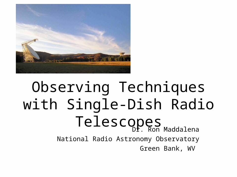
Typical Receiver

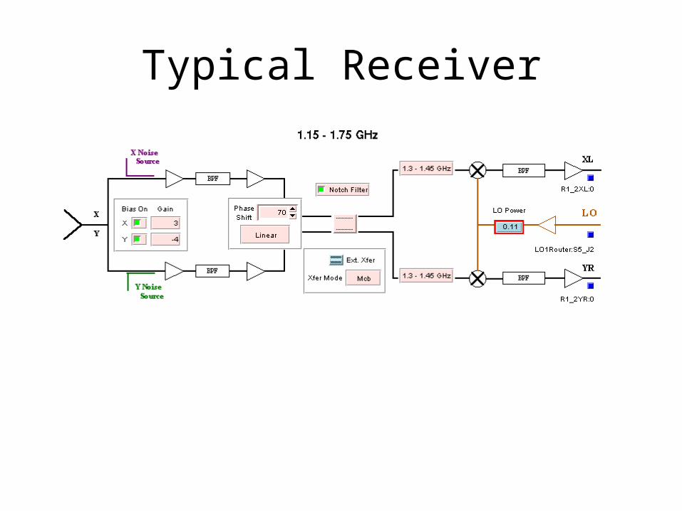
Dual Feed Receiver

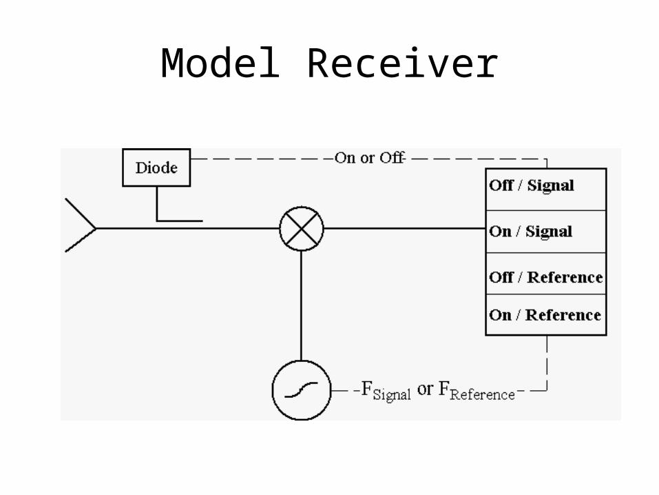
Model Receiver

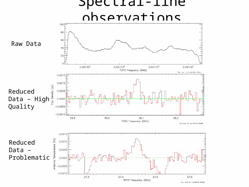
Spectral-line observations

Raw Data

ReducedData – HighQuality

ReducedData – Problematic

Reference observations

• Difference a signal observation with a reference observation

• Types of reference observations– Frequency Switching

• In or Out-of-band– Position Switching– Beam Switching

• Move Subreflector• Receiver beam-switch

– Dual-Beam Nodding• Move telescope• Move Subreflector

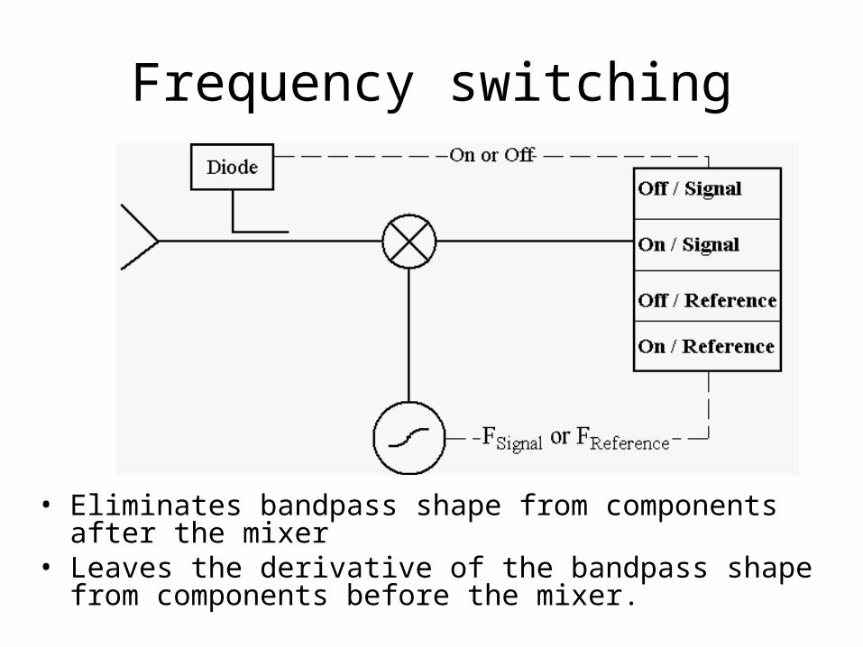
Frequency switching

• Eliminates bandpass shape from components after the mixer

• Leaves the derivative of the bandpass shape from components before the mixer.

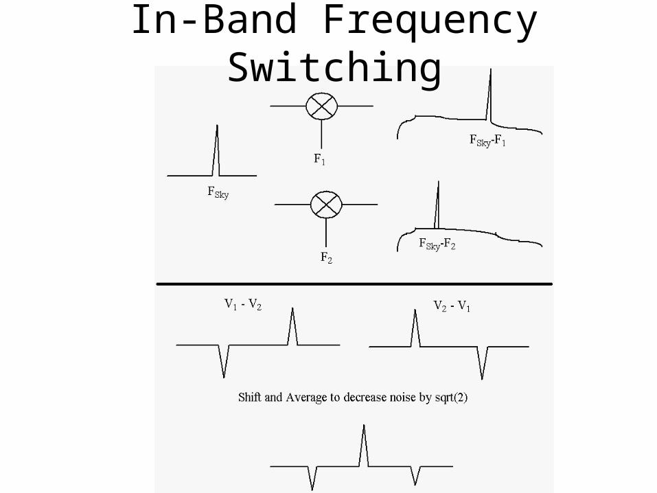
In-Band Frequency Switching

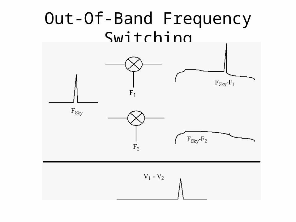
Out-Of-Band Frequency Switching

Position switching

• Move the telescope between a signal and reference position– Overhead– ½ time spent off source

• Difference the two spectra• Assumes shape of gain/bandpass doesn’t

change between the two observations.• For strong sources, must contend with

dynamic range and linearity restrictions.

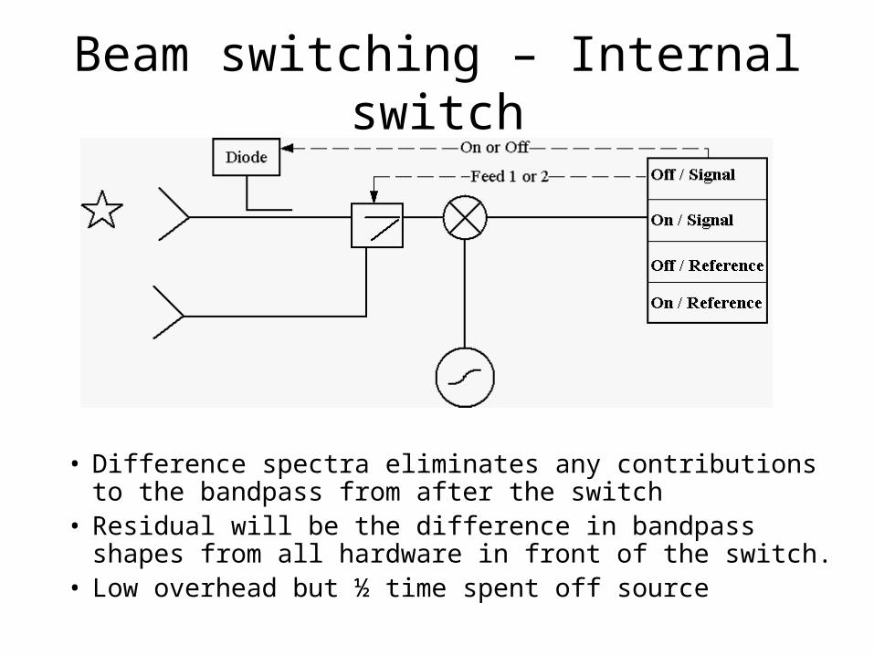
Beam switching – Internal switch

• Difference spectra eliminates any contributions to the bandpass from after the switch

• Residual will be the difference in bandpass shapes from all hardware in front of the switch.

• Low overhead but ½ time spent off source

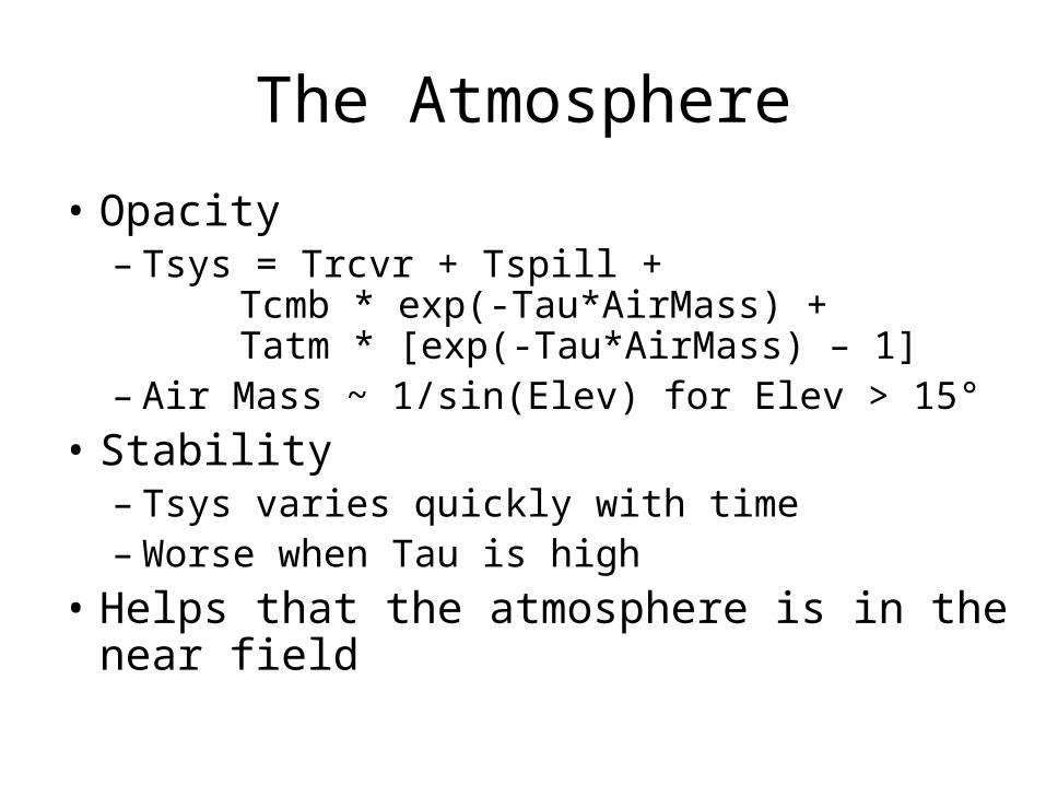
The Atmosphere

• Opacity– Tsys = Trcvr + Tspill +

Tcmb * exp(-Tau*AirMass) +Tatm * [exp(-Tau*AirMass) – 1]

– Air Mass ~ 1/sin(Elev) for Elev > 15°

• Stability– Tsys varies quickly with time– Worse when Tau is high

• Helps that the atmosphere is in the near field

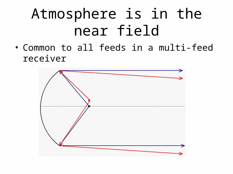
Atmosphere is in the near field

• Common to all feeds in a multi-feed receiver

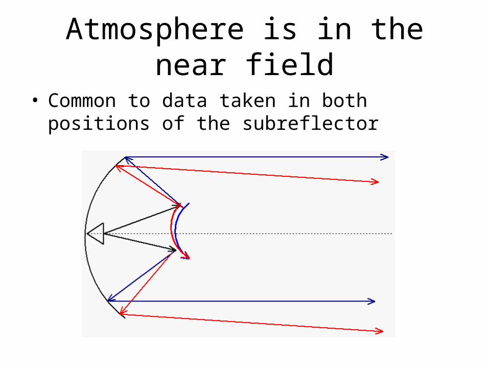
Atmosphere is in the near field

• Common to data taken in both positions of the subreflector

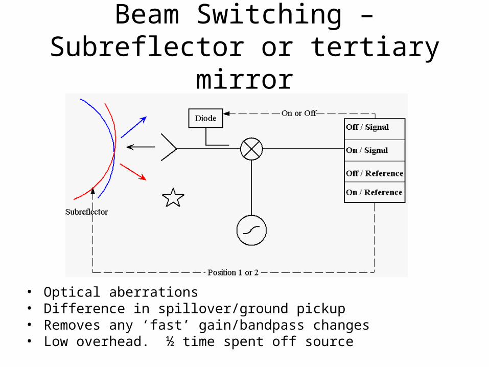
Beam Switching – Subreflector or tertiary mirror

• Optical aberrations• Difference in spillover/ground pickup• Removes any ‘fast’ gain/bandpass changes• Low overhead. ½ time spent off source

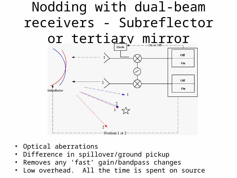
Nodding with dual-beam receivers - Subreflector or tertiary mirror

• Optical aberrations• Difference in spillover/ground pickup• Removes any ‘fast’ gain/bandpass changes• Low overhead. All the time is spent on source

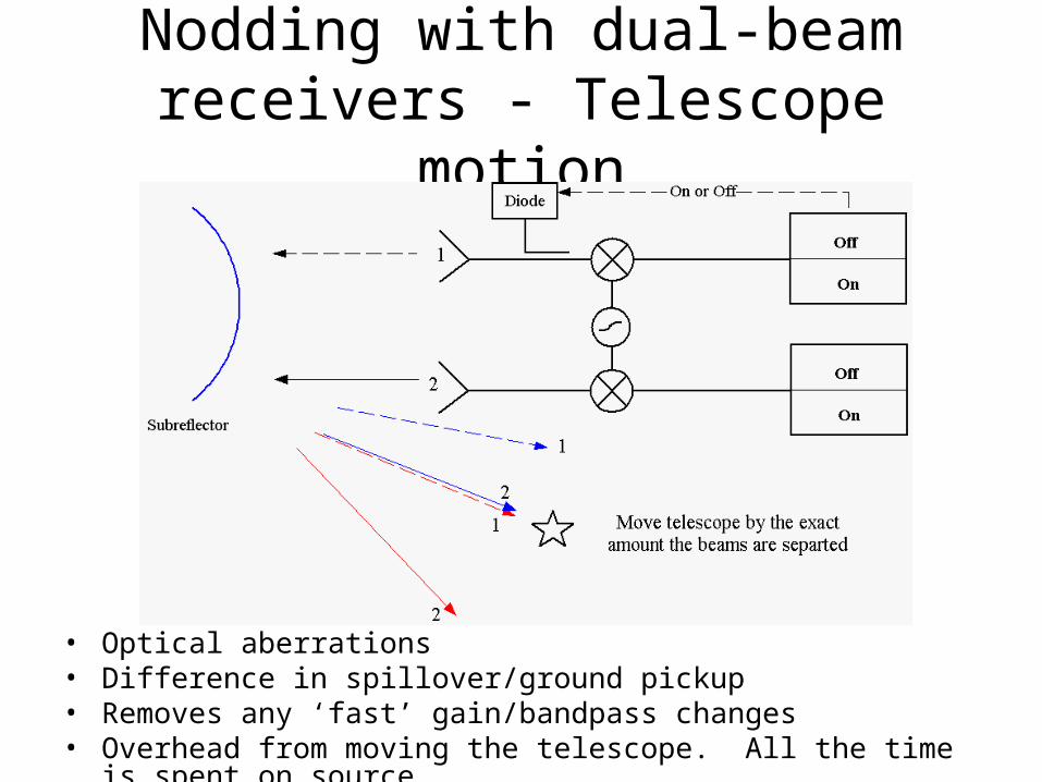
Nodding with dual-beam receivers - Telescope motion

• Optical aberrations• Difference in spillover/ground pickup• Removes any ‘fast’ gain/bandpass changes• Overhead from moving the telescope. All the time is spent on source

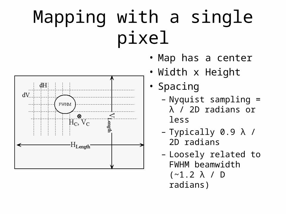
Mapping with a single pixel

• Map has a center• Width x Height• Spacing

– Nyquist sampling = λ / 2D radians or less

– Typically 0.9 λ / 2D radians

– Loosely related to FWHM beamwidth (~1.2 λ / D radians)

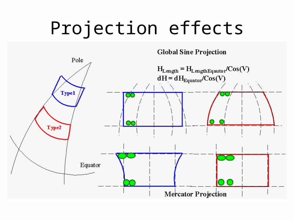
Projection effects

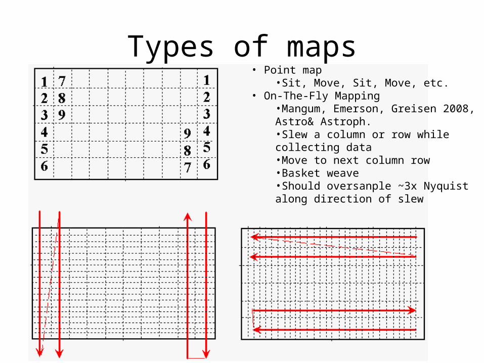
Types of maps• Point map

•Sit, Move, Sit, Move, etc.• On-The-Fly Mapping

•Mangum, Emerson, Greisen 2008, Astro& Astroph.•Slew a column or row while collecting data•Move to next column row•Basket weave•Should oversanple ~3x Nyquist along direction of slew

Other mapping issues

• Non-Rectangular regions

• Sampling “Hysteresis”

• Reference observations– Use edge pixels @ no costs– Interrupt the map– Built-in (frequency/beam switching, nodding,

etc.)

• Basketweaving

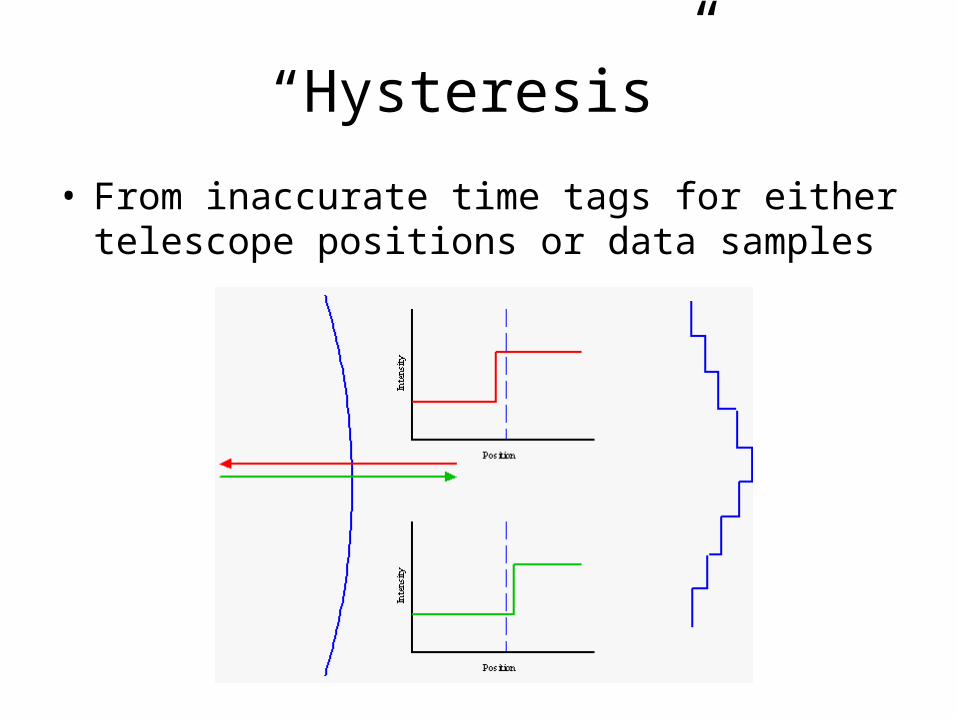
“Hysteresis”

• From inaccurate time tags for either telescope positions or data samples

Other mapping issues

• Non-Rectangular regions

• Sampling “Hysteresis”

• Reference observations– Use edge pixels @ no costs– Interrupt the map– Built-in (frequency/beam switching, nodding,

etc.)

• Basketweaving

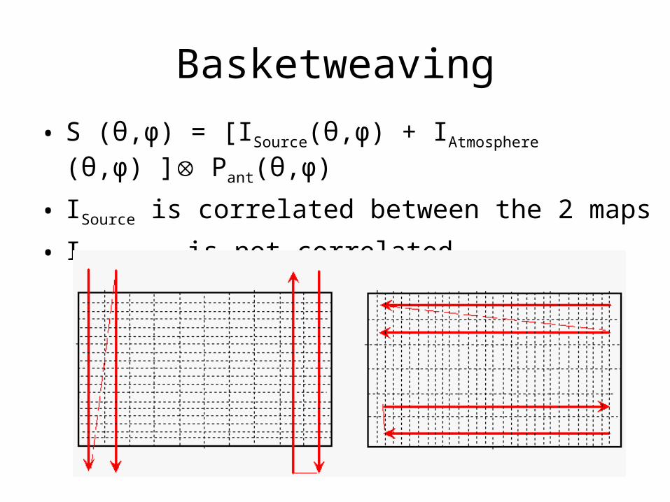
Basketweaving

• S (θ,φ) = [ISource(θ,φ) + IAtmosphere (θ,φ) ] Pant(θ,φ)

• ISource is correlated between the 2 maps

• IAtmosphere is not correlated

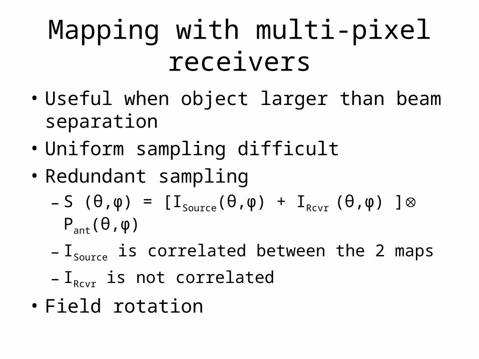
Mapping with multi-pixel receivers

• Useful when object larger than beam separation

• Uniform sampling difficult

• Redundant sampling– S (θ,φ) = [ISource(θ,φ) + IRcvr (θ,φ) ] Pant(θ,φ)

– ISource is correlated between the 2 maps

– IRcvr is not correlated

• Field rotation

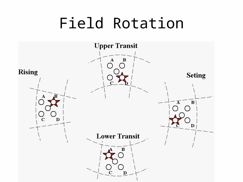
Field Rotation

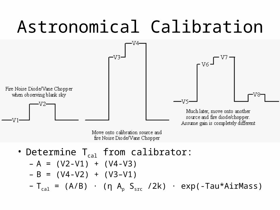
Astronomical Calibration

• Determine Tcal from calibrator:– A = (V2-V1) + (V4-V3)– B = (V4-V2) + (V3–V1)– Tcal = (A/B) ∙ (η Ap Ssrc /2k) ∙ exp(-Tau*AirMass)

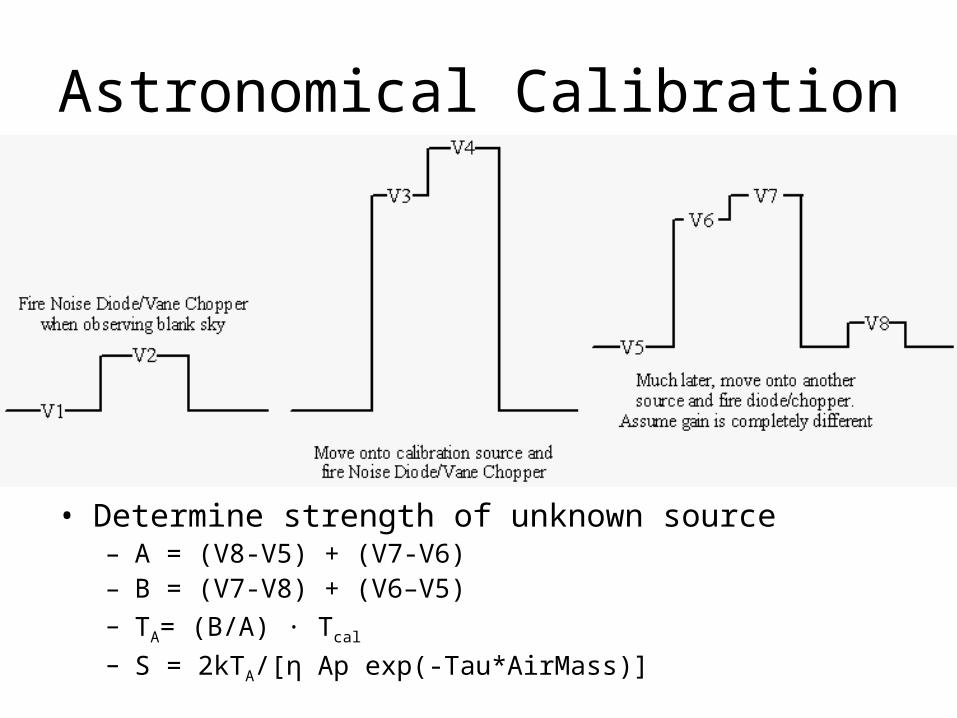
Astronomical Calibration

• Determine strength of unknown source– A = (V8-V5) + (V7-V6)– B = (V7-V8) + (V6–V5)– TA= (B/A) ∙ Tcal

– S = 2kTA/[η Ap exp(-Tau*AirMass)]

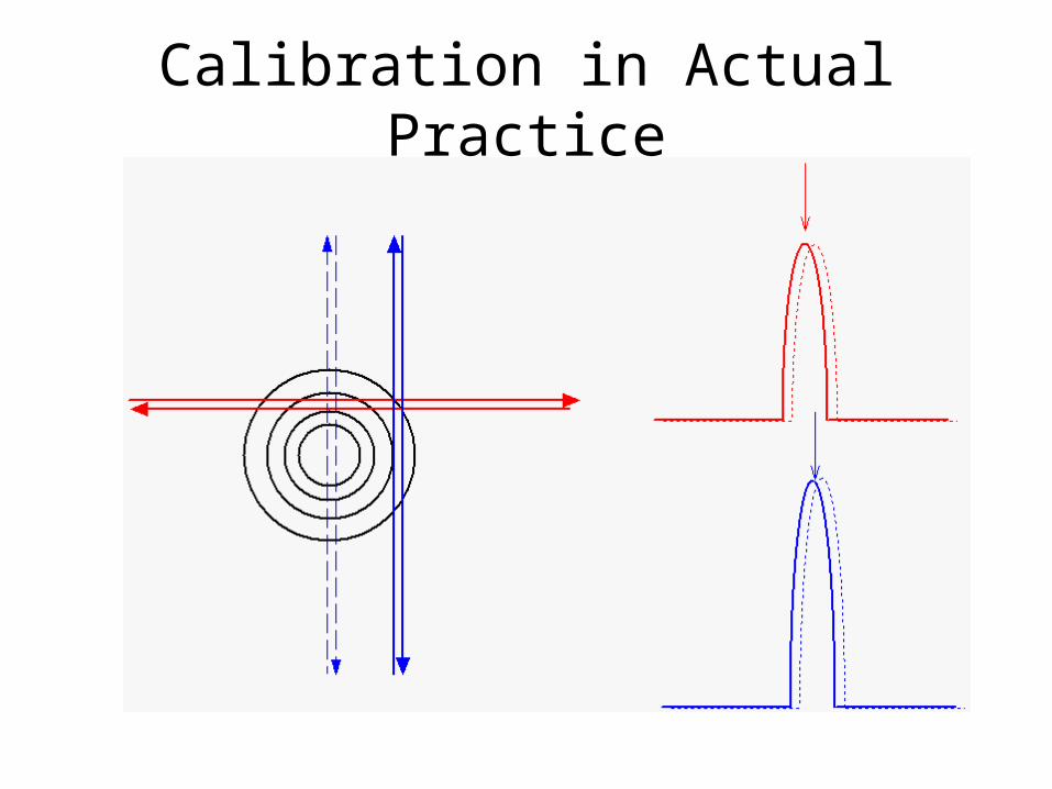
Calibration in Actual Practice

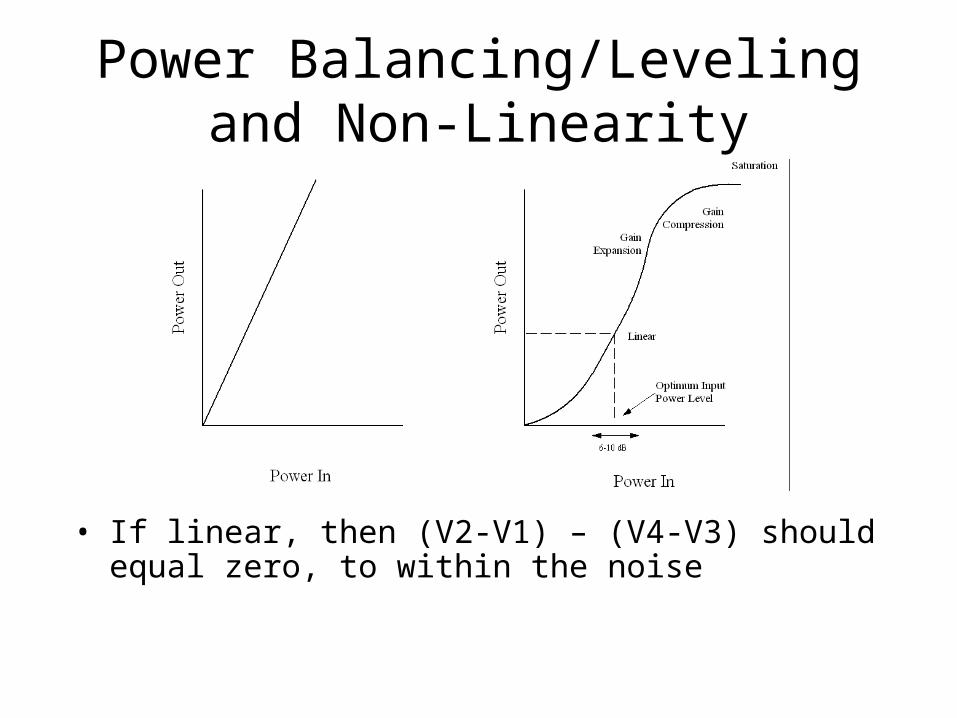
Power Balancing/Leveling and Non-Linearity

• If linear, then (V2-V1) – (V4-V3) should equal zero, to within the noise

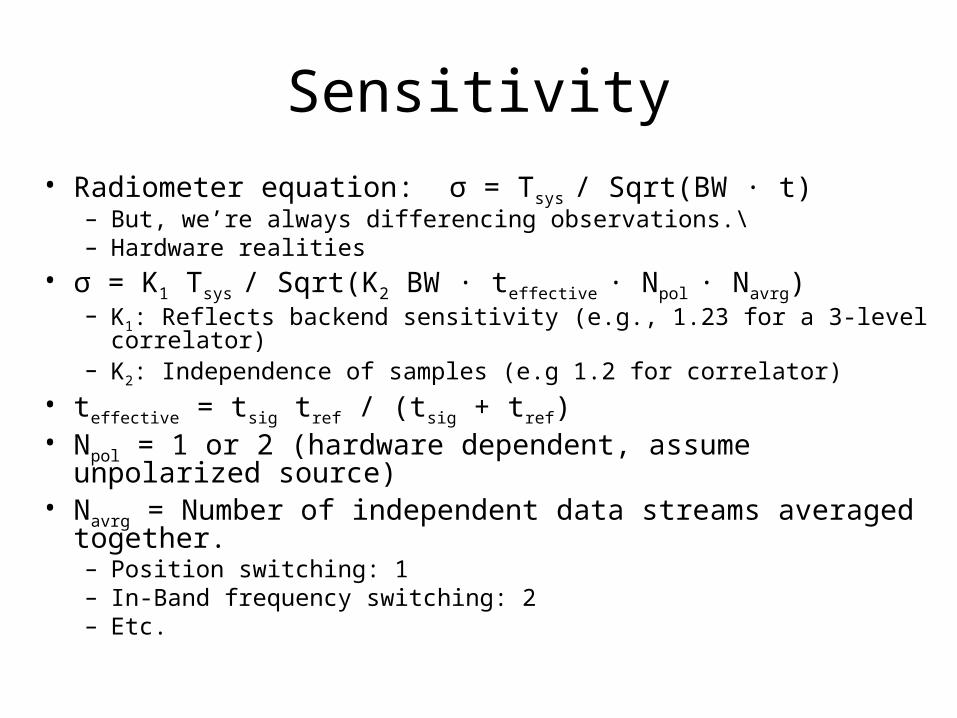
Sensitivity

• Radiometer equation: σ = Tsys / Sqrt(BW ∙ t)– But, we’re always differencing observations.\– Hardware realities

• σ = K1 Tsys / Sqrt(K2 BW ∙ teffective ∙ Npol ∙ Navrg)– K1: Reflects backend sensitivity (e.g., 1.23 for a 3-level correlator)– K2: Independence of samples (e.g 1.2 for correlator)

• teffective = tsig tref / (tsig + tref)• Npol = 1 or 2 (hardware dependent, assume unpolarized source)• Navrg = Number of independent data streams averaged

together.– Position switching: 1– In-Band frequency switching: 2– Etc.