Observations of high-frequency internal waves in …oxbow.sr.unh.edu/preprints/internalwaves_obs.pdf · Observations of high-frequency internal waves in the ... it can a ect diapycnal

1

Observations of high-frequency internal waves in the

Coastal Ocean Dynamics Region

James M. Pringle1

Woods Hole Oceanographic Institution, Woods Hole, Massachusetts, 02543

Abstract. Current meter data from the second Coastal Ocean Dynamics Experi-ment (CODE II) for July 1982 are analyzed for internal waves in the 6 to 40 cyclesper day (cpd) frequency band. It is found that the wave field is anisotropic and thatthe current ellipses are oriented in approximately the cross-isobath direction. Thesquares of the ratio of the major to minor axes of the current ellipses (the “elliptic-ity”) are consistent with a continuum of internal waves propagating onshore but arenot consistent with a single wave propagating onshore. The reduction of internalwave energy across the shelf is consistent with propagation from the deep ocean orshelf break, as is the correlation between vertical velocities and velocities parallel tothe minor axis. However, there is evidence for the generation of additional internalwave energy on the shelf in the evolution of the current ellipses across the shelf andin the bluing of the internal wave spectra across the shelf. Internal wave energylevels are elevated by a factor of 1.5 to 5 above Garrett and Munk [1972] levels atthe moorings on the 130 and 365 m isobaths. The first vertical mode dominatesat the 130 m isobath, the only mooring for which the vertical modal analysis wasdone.

1. Introduction

In the deep ocean, away from horizontal and verticalboundaries, the high-frequency internal wave spectrumis well modeled by the Garrett and Munk [1972] spec-trum (hereafter referred to as GM). In shallow coastalregions there is no such universal description of theinternal wave field. Thus it is useful and interestingto examine the internal wave climate at a particularshelf location. The current meters and thermistors de-ployed during the Coastal Ocean Dynamics Experiment(CODE) allow one to examine how the high-frequencyinternal wave spectrum changes across a continentalshelf. This is done for the central current meter ar-ray of the CODE II experiment for the month of July1982. An accompanying study by Pringle and Brink[this issue] (hereafter referred to as PB) models linearinternal wave propagation from the shelf break to thecoast using a GM spectrum as the deep ocean initialcondition. To the extent that the observations and the-ory can be compared and differ, it gives an idea of howmuch of the internal wave energy on the shelf is gen-erated on the shelf and how much propagates in fromthe ocean. A detailed comparison of PB and the datais impossible because the data are unable to resolve thehorizontal wave number spectrum of the internal waves,

2

and the internal wave spectrum in the ocean adjacentto the shelf is also unknown.

For the CODE region, high-frequency waves havebeen defined, somewhat arbitrarily, as those with fre-quencies between 6 and 40 cycles per day. This range offrequencies is between the highest frequency of criticaltopographical reflection of internal waves (6 cpd) andthe lowest buoyancy frequency observed on the shelf forthe time of the analysis (40 cpd). The month of July1982 was chosen because the stratification was relativelyconstant throughout the month and the hydrographicstructure was generally simple. The same analysis aspresented herein can be performed for other times inthe data record. The results do not seem qualitativelydifferent, but the analysis is difficult because of the un-certainties in calculating the stratification at the currentmeters in other months.

The high-frequency internal wave climate on the shelfis interesting, not only in its own right but also becauseit can affect diapycnal mixing [Sandstrom and Elliott,1984; Sanford and Grant, 1987] and the propagationof acoustic energy on the shelf [Lynch et al., 1996]. Ithas been studied by several authors, including Gordon[1978], who analyzed internal waves using current meterdata taken off Spanish Sahara at 21◦N, 17◦W as part ofthe 1974 JOINT-1 experiment. That shelf has a bottomslope, 2 × 10−3, between those typical of the east andwest coasts of North America. Gordon concluded froman empirical orthogonal function analysis that most ofthe energy is in the first-mode internal waves and thatthose waves propagated toward the shore. He claimedthat energy dissipation was dominated by the effects ofshoaling as the waves entered shallow water and by thesubsequent nonlinear dissipative effects of wave break-ing.

Another analysis of internal wave data by Howell andBrown [1985] is of interest because it was done at thesame site as the present analysis. Howell and Brownanalyzed six internal wave soliton events that occurredduring a six day period in April 1981. They concludethat they did observe solitons with a period of about25 minutes, and that the events corresponded well withtwo-layer soliton theory. Howell and Brown’s conclu-sions would have to be included in any more completeanalysis of internal waves on the shelf.

2. Internal Wave Background

Garrett and Munk [1972] codified the deep water in-ternal wave spectrum, and their scheme has proven tobe surprisingly robust away from horizontal boundaries,vertical boundaries, and the equator [Wunsch, 1976].

3

There is no reason to expect that it will be correct onor near the shelf. However, since deep ocean internalwaves may propagate onto the shelf and since whateverprocesses maintain the deep ocean at the GM spectrummay also drive the coastal internal wave spectrum lo-cally, the GM spectrum makes a useful point of refer-ence for any observed spectrum. In PB the propagationof a GM spectrum onto the shelf is explicitly modeled,but whatever nonlinear processes equilibrate the GMspectrum in the deep ocean are not considered.

The GM spectral power density is, for horizontal cur-rents observed by a current meter that moves with thesubinertial current,

⟨u2⟩

+⟨v2⟩

= (4Eb2N0)Nfω−3 ω2 + f2

√ω2 − f2

, (1)

where (4Eb2N0) is a scale power spectral density of 2.2m2s−1;

⟨u2⟩

and⟨v2⟩

are the volume-averaged hori-zontal current variances; and N , f , and ω are the localbuoyancy, inertial, and internal wave frequencies, re-spectively. When ω2 � f2, the power spectrum can besimplified to

⟨u2⟩

+⟨v2⟩

= (4Eb2N0)Nfω−2 (2)

with very little error.Wunsch [1968,1969] and McKee [1973] examined in-

ternal waves propagating in a uniformly stratified wedge.The McKee solutions show that incoming internal wavecrests turn to parallel the beach in the same way thatsurface gravity waves do. They also derive the slope cfor critical internal wave reflection off the bottom:

c =

√ω2 − f2

N2 − ω2(3)

If the bottom slope is steeper than c, the wave will bereflected back to deeper water. If the slope is less than0.5c, the bottom appears locally flat, and if the slopeis nearly equal to c, a region of strong shear will existnear the bottom.

3. Topography and Coordinates

The CODE region, which is described by Beards-ley and Lentz [1987], is centered around 123◦30W and38◦30N, between Point Arena and Point Reyes, Califor-nia. Figure 1 shows the location of the current meter Figure 1moorings used in the present analysis. The coastlineis straight for about 75 km, the straight portion beingapproximately centered on the central (“C”) moorings.The alongshore and cross-shelf directions are defined

4

by the mean orientation of the coast around the cen-tral array; the cross-shore axis points to 47◦T, and thealongshore axis points to 317◦T. [Beardsley et al., 1985].The shelf break, however, is not parallel to the shore.A coordinate system defined by the 365 m isobath isrotated by about 17◦ clockwise from the coordinatesystem defined at the shelf.

The shelf break is at about 200 m, and the slope ofthe shelf averages 5×10−3 between C4 and C3 (130 and90 m depth, respectively) and 5× 10−2 at C5. C5 is in365 m of water, beyond the shelf break at 200 m.

Wunsch [1969] solves for the characteristic slope of aninternal wave. If the bottom slope is greater than thecharacteristic slope of an internal wave, the wave can nolonger be represented with vertical modes and internalwave energy reflecting off the bottom will be sent backto the deep sea (PB). Since much of the analysis hereconsiders the propagation of internal waves from thedeep ocean onto the shelf, the analysis will be restrictedto frequencies whose characteristic slope is everywheregreater than the bottom slope. This is true when

ω >

√f2 + α2N2

1 + α2≈√f2 + α2N2, (4)

where α is the bottom slope. An N of 100 cpd, an fof 1.24 cpd, and a maximum bottom slope on the shelfbreak of 6 × 10−2 restricts the analysis to frequenciesgreater then 6 cycles per day. This also avoids internalwaves at the tidal and inertial frequencies, whose forc-ing mechanisms are likely to be different than the forc-ing mechanisms of the higher-frequency internal waves.The critical frequency on the shelf, with its slope of5× 10−3, is only 5% higher than f , and so is not nearthe frequencies analyzed here.

4. Hydrography

The month of July 1982 was chosen for analysis be-cause the hydrography had a simple relationship be-tween temperature and density, which allows the calcu-lation of density σ from the temperatures T observed atthe current meters. The overall hydrography is typifiedby Figure 2, an average for the April to July upwelling Figure 2season (Figure 2 is drafted from Kosro and Huyer [1986,Figure 24]). It is similar to the two sections taken onJuly 16 and 19, 1982, and the many other conductivity-temperature-depth (CTD) casts taken in July [Huyer etal., 1983].

A relation between temperature and potential densitywas formed from the CTD casts taken during July in theCODE region on the shelf and shelf break. Only data

5

from less than 400 m were used to obtain the relation

σ = −0.1781T + 27 T < 7.74◦C (5a)

σ = −0.2633T + 28 7.74◦C < T < 9.212◦C (5b)

σ = −0.1975T + 28 T > 9.212◦C (5c)

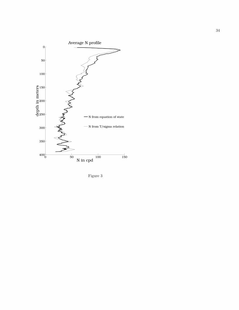
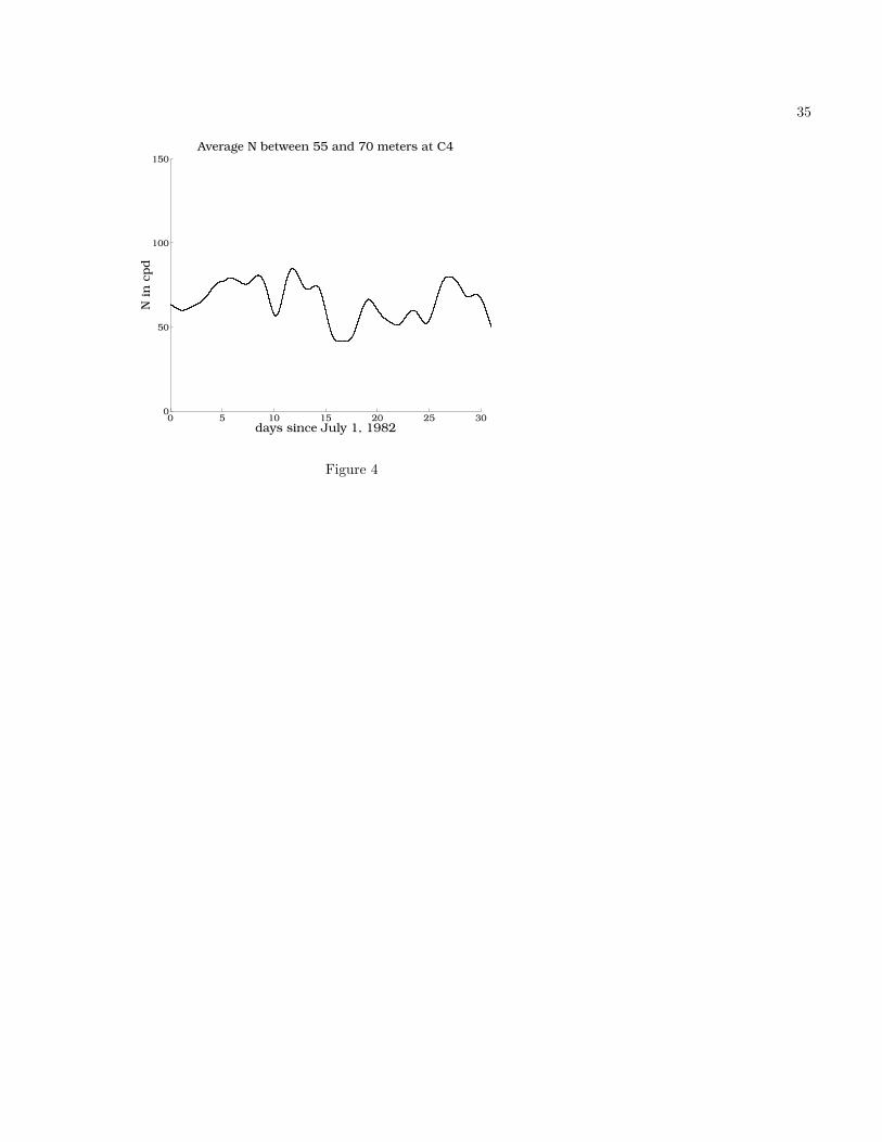
This includes both the effect of the nonlinearity of theequation of state and the observed T/S relation. TheRMS difference between (5) and the density computedwith the full equation of state is 0.085 kg m−3. To pro-vide confidence in this empirical relation, the buoyancyfrequency from the CTD sections is plotted as computedfrom the full equations of state and as computed from(5a)-(5c) (Figure 3). Though not a rigorous test, since Figure 3it uses the same data as used to derive the σ/T rela-tion, it is reassuring that there are few outliers. Thisσ/T relation allows one to compute densities from thetemperature records at each current meter. A represen-tative middepth time series of N2 is shown for the waterbetween 55 and 70 m at the C4 mooring in Figure 4. Figure 4The temperature data used for Figure 4 were low-passfiltered with a half-amplitude pass at 3.25 times the in-ertial period (f=1.24 cpd) and a full-amplitude pass at4 times the inertial period. This removes the displace-ments in the density field caused by the internal waves.

5. Low-Frequency Currents

Unfortunately, the high-frequency data needed tostudy internal waves were only archived for the moor-ings at the 130 and 365 m isobaths. There are onlyhourly data available for the moorings shoreward of130 m. Thus most of the following analysis can onlybe done with the C5 mooring in 365 m of water andthe C4 mooring in 130 m of water. The C4 mooringhad usable current meters at 10 and 20 m on a surfacemooring and at 35, 55, 70, 90 and 121 m on a subsurfacemooring 100 m away. The C5 mooring had instrumentsat 20, 35, 55, 70, 90, 110, 150, 250, and 350 m [Beardsleyet al., 1985].

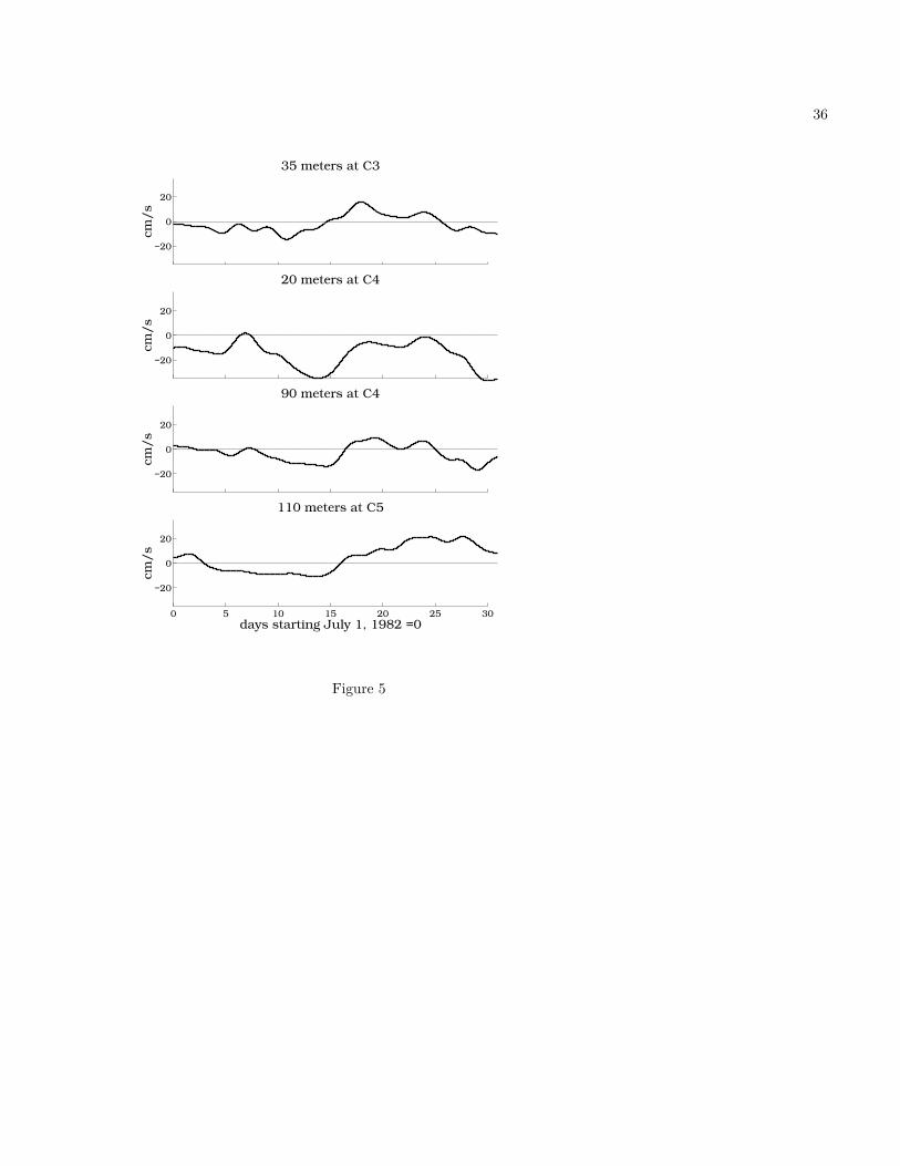
The alongshore subinertial currents during July hadtwo main characteristics. At the 90 m (C3) and 365 m(C5) moorings, alongshore flow was equatorward (v ≈−5 to −15 cm s−1) for the first 15 days of the monthand poleward the next 16 days (v ≈ 5 to 15 cm s−1).This was also true of the alongshore currents at 90m and below at the 130 m (C4) mooring. However,the currents were persistently equatorward in the waterabove 90 m at C4. The cross-shelf currents were lessvigorous than the alongshore currents. The barotropiccurrent at C4 is equatorward for the first 15 days andnearly zero for the next 15 days. Figure 5 shows plots of Figure 5

6

representative alongshore currents at C3, C4, and C5.For more information on the low-frequency currents, seeWinant et al. [1987].

6. Analysis at Individual CurrentMeters

The GM model makes three strong statements aboutthe internal wave spectrum in the deep ocean. Theshape of the power spectrum of horizontal currents goesroughly as ω−2, the energy level is fixed, and the spec-trum is isotropic. However, it will be shown below thatthe shape of the internal wave spectrum on the shelfvaries across the shelf, the internal wave energy levelsvary with mooring and time, and the spectra are neverisotropic.

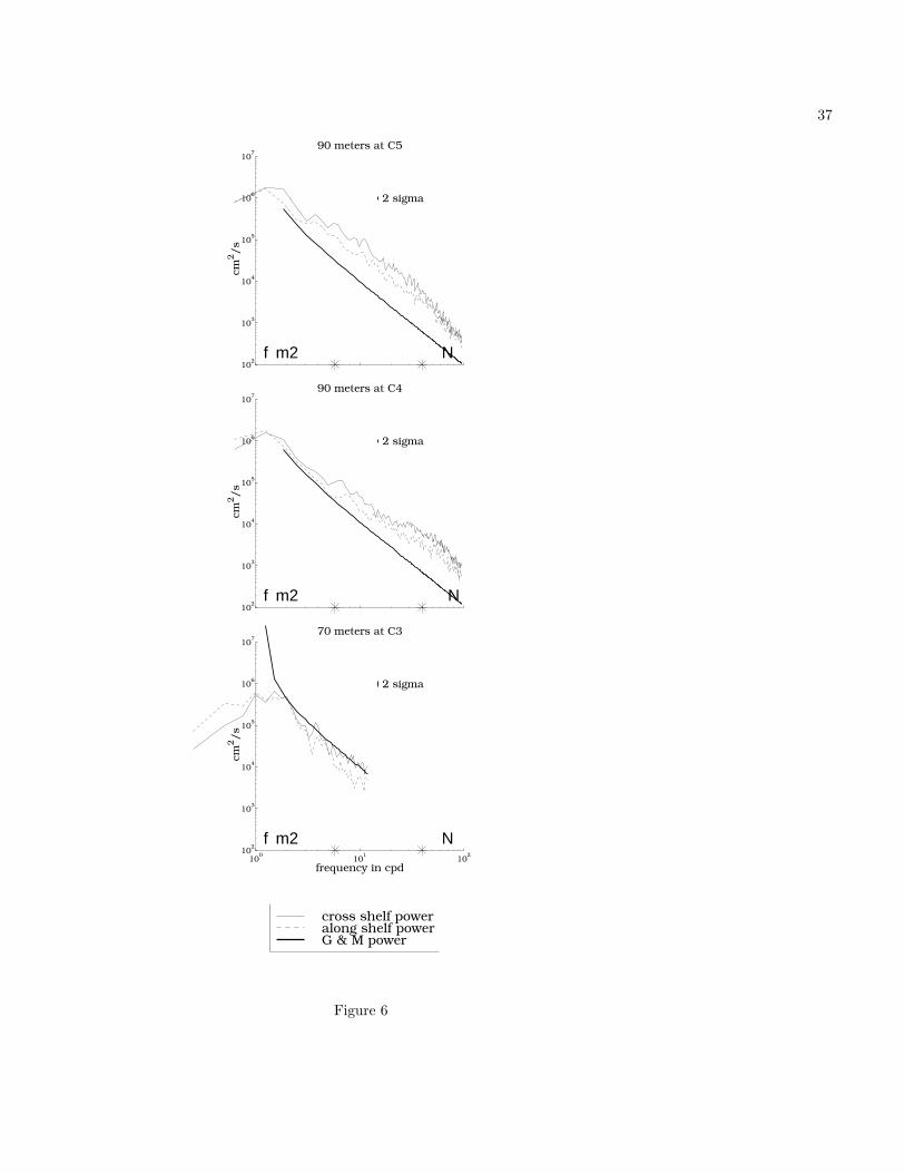
Figure 6 shows power spectra of velocity from the Figure 6C5, C4, and C3 moorings, at depths chosen becausethey illustrate well the general trends of the spectra.The power spectra are computed with half-overlappedWelsh windows of period 4π/f , so that the spectra re-solve the full internal wave band including tidal andinertial frequencies (though these peaks are not promi-nent in the data). The spectra become less red as onemoves onshore, the energy levels decrease, and the cur-rent ellipses are not the circles that GM predicts for thedeep ocean. In section 7 it will be shown with energyarguments that the high-frequency data are consistentwith internal waves.

6.1. Horizontal Current Kinetic Energy

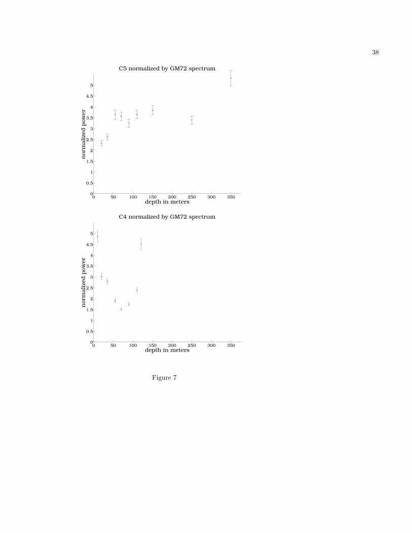
The total mean square current, u2 +v2, in the 6 to 40cpd wave band is plotted for current meters C4 and C5in Figure 7. The mean square current has been scaled Figure 7by the GM spectrum for the time-averaged buoyancyfrequency, so a value of 1 would match the kinetic en-ergy in the GM spectrum. The power at both locationsis consistently larger than the GM power. The powerat the C5 mooring is greater than at the C4 mooring,both when integrated over the water column and aver-aged over the water column. The depth-averaged poweris reduced by a factor of about 1.5 between C5 and C4,while the depth-integrated power is reduced by about4, which is consistent with the frictional dissipation ofshoreward propagating internal waves as described byBrink [1988] and modeled in PB, and it strongly sup-ports the idea that most of the internal wave energyon the shelf is propagating in from the deep ocean orshelf break and being dissipated as it moves shoreward.If energy were propagating adiabatically from offshore,both the power integrated over the water column and

7

the power per vertical distance should increase towardthe shore as the waves shoal (PB). If the waves werepropagating from the coast outward, the power shouldlikewise increase shoreward, with or without friction,because both friction and shoaling work to reduce theenergy in the wave as it moves offshore. Thus the reduc-tion of internal wave power as one moves closer to theshore is a robust indication that energy is propagatingfrom the deep ocean or shelf break and is being dissi-pated as it moves to the shore. The limited amount ofdata at the 90 m C3 mooring (Figure 6) indicates thatthe internal wave energy continues to decay across thecoast, again consistent with PB.

The enhanced energy near the surface and the bot-tom at C4 suggests that the internal waves there aredominated by the first baroclinic mode, which is con-sistent with the modal analysis presented below. Thelack of a similar enhancement at C5 argues that mode1 is not dominant in the deeper water.

6.2. Spectral Shape

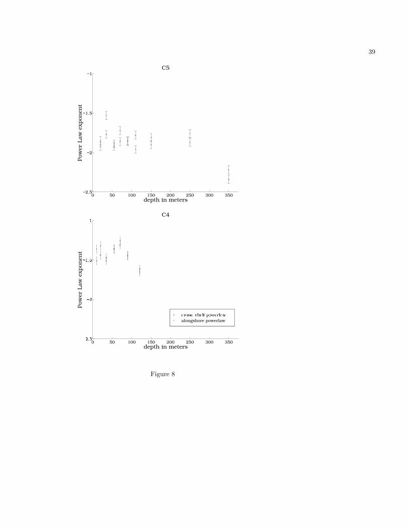
In Figure 6 one can see that the log-log spectralslope becomes less steep as one moves toward the shore.This is confirmed by Figure 8, which shows the spectral Figure 8slopes at all the current meters on the 365 m and 130 mmoorings. The slope is computed from a linear leastsquares fit between the log of the power and the log ofthe frequencies analyzed. There were not enough spec-tral data to analyze robustly the power laws at the C3site. The slopes at the 365 m mooring are around 1.8,except for the deepest current meter, where the slopeis steeper. The slopes for the 130 m mooring clusteraround 1.5. Since the 1 standard deviation uncertaintyof the fits is less than 0.06, these slopes are significantlydifferent. The reduction of the slope of the shallow wa-ter spectra is puzzling if one views the internal waves aspropagating in from the deep sea. Since the waves decayat a roughly constant rate per unit time [Brink, 1988;Sanford and Grant, 1987; PB], one would expect thehigh-frequency waves, which are slower, to be dissipatedmore strongly per unit distance as they move onshore.This would redden the spectrum by selectively dissipat-ing the higher-frequency waves. The resolution of thisdiscrepancy may lie in a conjectural nonlinear interac-tion that transfers energy from low-frequency waves tohigher-frequency waves or in the preferential generationof high-frequency internal waves on the shelf or shelfbreak. For instance, the high-frequency internal soli-tons found by Howell and Brown [1985] could, if gen-erated between the 365 m and 130 m site, account forsome of the extra high frequency energy. The relative

8

excess of high-frequency energy over low is the greatestdisagreement between PB and the data.

6.3. Lack of Isotropy: Predictions From PB

The GM spectrum is isotropic, but it is no surprisethat the internal wave spectrum has a strong polar-ization near the coast. McKee [1973] studied internalwaves propagating into a wedge-shaped topography. Henoted that internal wave crests turn to parallel the coastas surface gravity waves do. This tends to focus thewave energy toward the coast.

If the internal waves start at the shelf break with nopreferred orientation, those that propagate toward thecoast turn, so that their crests become more parallelto the coast. Since internal waves have current ellipseswhose major axes are oriented in the direction the wavesare propagating, this turning toward the coast tendsto make the current ellipses perpendicular to the localbathymetry.

If the waves are generated near the shore and radiateoutward, their orientation depends sensitively on thesource location and the orientation of the waves gener-ated at the source. Since current ellipses are symmetricaround their major and minor axes, the shape of theellipse does not indicate whether a wave is coming onor offshore. Waves that are generated at the shore butradiate at an angle to the shore will be trapped shore-ward of a depth that decreases as the magnitude of theangle to the normal of the shore increases. The ellipseorientation of a trapped wave depends sensitively on thetrapping depth and varies as the wave crosses the shelf,and so it depends sensitively on the source geometry.

A mean flow can also alter the internal wave geom-etry. There are many possible effects. Current shearalters the local relative vorticity and hence the appar-ent f [Kunze, 1985]. The internal wave can trade en-ergy back and forth with the mean current [Lighthill,1978]. The effect that is found in PB to be dominantat these frequencies and for realistic mean currents isthe effect of Doppler shifting a red spectrum. A currentwill Doppler shift the observed wave, so waves travelingwith the mean current will be observed at frequencieshigher than their intrinsic frequency, and those travel-ing against the current will be observed at lower thantheir intrinsic frequency. If the spectrum of the inter-nal waves in the reference frame of the mean currentis red, as it almost certainly is, then the amplitude ofthe waves traveling with the current, which have lowerintrinsic frequencies, will be greater. Because of this,the current ellipse will be shifted in the direction of thecurrent.

9

All of these effects operate at the same time, so dis-tinguishing the relative contributions of each in the datais hard. PB presents a model of these effects for wavesof a GM spectrum at the shelf break propagating overthe shelf. The model uses ray tracing to follow thehorizontal path of internal wave vertical modes and as-sumes that near the shelf break the path of the inter-nal waves becomes controlled by the bathymetry. Thisnaive treatment of the shelf break, as well as the lackof any alongshore variation in currents and the disre-gard of any nonlinear effects other than wave interac-tion with a mean flow, are the primary weaknesses ofthe model. However, its simplicity has the advantagethat its predictions can be easily summarized as fol-lows: (1) Topographic refraction makes the major axisof the current ellipses perpendicular to the isobaths. (2)The ellipticity of the current ellipse, which is the ratioof the horizontal current power in the major axis di-rection to the power in the minor axis direction, willincrease closer to shore but will not depend stronglyon wave frequency. Currents of the magnitude seen inthe CODE region will not greatly change the ellipticity.(3) The current will tend to shift the major axis of thecurrent ellipse downstream, that is for a positive meancurrent the angle of the major axis to the cross-shoredirection is positive (see Figure 9). For a bathymetry Figure 9such as that in the CODE region, the mean currentswill shift the major axis of the current ellipse of verticalmode 1 and mode 2 waves by only 5 to 15◦away fromthe cross-isobath direction for mean currents less than20 cm s−1.

In order to disentangle the effects of topography andalongshore current in the data, two types of analysiswill be performed. First, the ellipticity and orientationof the currents as a function of frequency for each cur-rent meter will be analyzed for two time subperiods,one for when the mean currents were predominantlypoleward, one for when they were predominantly equa-torward. Then, since the predictions of the effects of thealongshore current depend on the vertical mode struc-ture of the wave, a similar analysis will be done on thethe modally decomposed data. It is also with this de-composition that the direction of propagation of thewaves can be determined, and the power in the verti-cal and horizontal currents can be compared to internalwave theory.

6.4. Ellipticity

One observable that indicates anisotropy is the squareof the ratio of the major to minor axis of the currentellipse (the “ellipticity”). This is the ratio of the powers

10

in the horizontal currents in a coordinate system alignedwith the major axis. For a single plane wave it varieswith frequency as ω2/f2. For an isotropic spectrumon an f plane, it is, of course, 1. The theory in PBpredicts that the ellipticity of a continuum of waves overthe shelf should not be a function of vertical mode andonly a weak function of ω and mean currents, until nearthe coast when all the waves have been topographicallyrefracted to be nearly perpendicular to the coast or untilthe mean alongshore currents become strong enough toabsorb or reflect the waves, neither of which occurs atthe C4 or C5 sites.

In order to collapse the data at each current meterin each subperiod into a single number, the ellipticity iscalculated for each frequency between 6 and 40 cpd, andthose ellipticities are averaged with a constant weight-ing, ignoring the differences in energy at each frequency.Since the spectra are red, any power-weighted averageis approximately the ellipticity at 6 cpd and thus notmuch more useful than only examining the ellipticity at6 cpd. The averages are therefore made without powerweighting in order to increase the robustness of the sta-tistical tests applied to the averages. Averaging theellipticity over a range of frequencies is a sensible thingto do for a random isotropic wave spectrum, for eachfrequency is an independent sample. However, averag-ing the observed ellipticity over a range of frequencies isstill troublesome, for any nonlinear interaction betweenthe waves could introduce correlations between mea-surements made at different frequencies. Nonetheless,there is no consistent variation of ellipticity with fre-quency for various current meters, an observation thatagrees with the result in PB that ellipticity should be aweak function of ω. This can be seen in the spectra inFigures 6 and 10, in which there are no consistent varia- 10tions in the ratio of the power spectra of the cross-shoreand alongshore velocity in the 6 to 40 cpd frequencyrange.

As an observed quantity, ellipticity is difficult to an-alyze, for any random time series of currents will havean ellipticity of 1 or greater. Thus the sample aver-age ellipticity of an observed isotropic spectrum will begreater than 1, even though the expected average willasymptote to 1 as the length of the record increases.However, for this analysis the ellipticity at a given fre-quency is different from an isotropic spectrum with 80%confidence if its ellipticity is greater then 1.37, and theaverage ellipticity over the 6 to 40 cpd frequency bandconsidered here is different from an isotropic spectrumat the 95% level if the ellipticity is greater then 1.37.That both significance levels are 1.37 is a coincidence.

11

These significance levels were found by a Monte Carlotechnique: the distributions of ellipticity from 105 syn-thetic isotropic time series was computed, and from thisthe confidence levels were obtained.

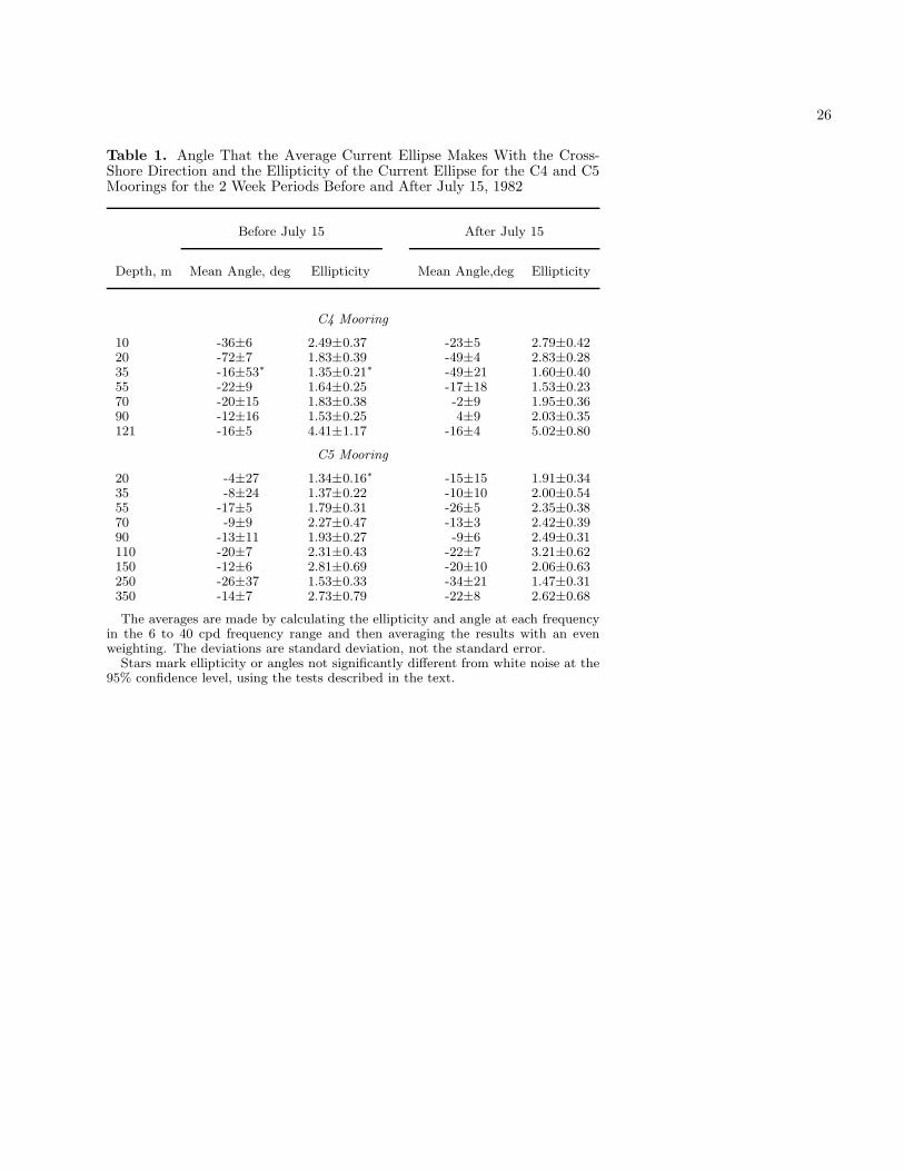
Only one of the 32 estimates of the average ellipticityof the data in Table 1 fails to be different from white Table 1noise at 95% confidence, so the data must be consid-ered anisotropic. The average ellipticities in Table 1 liebetween 2.8 and 1.4, except for the bottommost currentmeter at C4, whose ellipticity is ≈ 4.75 for the wholerecord. At C4 the ellipticities are enhanced near the topand bottom to levels that are near the levels that willbe obtained for the mode 1 waves in the modal decom-position below. This is consistent with the idea thatthe internal wave energy at C4 is dominated by mode1 and suggests that this is not true for C5. None ofthe current records has ellipticities near the ω2f−2 pre-dicted for a single internal wave, so the internal wavefield cannot be made up of a single wave propagatingin from the shelf break, but the results are consistentwith an ensemble of internal waves propagating acrossthe shelf.

PB predicts that if all of the internal waves on theshelf had originated as an isotropic wave field in thedeep ocean, the ellipticity of the current ellipses shouldincrease as the waves move toward the coast. This isnot observed, again suggesting that there is wave gen-eration or modification on the shelf. Waves generatedon the shelf would also tend to be turned toward thecoast by the topography and thus become consistentwith the PB picture closer to shore. A more detailedcomparison to the model in PB is not practical, forthere is not enough information in the current meterrecords to compute the horizontal wave number spectraat the current meter moorings, and thus it is impossi-ble to compensate for the naivete of PB’s internal waveboundary conditions at the shelf break or to diagnosewhat waves are generated on the shelf or at the shelfbreak between C5 and C4.

Interestingly, 13 out of 16 current meters at C5 andC4 had greater ellipticities in the second half of themonth, when the water was flowing poleward or lessequatorward. The PB model does not predict this ef-fect, which may be caused by alongshore variation inthe mean flow or localized generation of internal waveson the shelf or shelf break.

6.5. Current Ellipse Orientation

From the angle of the major axis of the current ellipseto the cross-shore direction, one can get a good con-straint on the direction of propagation of energy since

12

the current ellipse, horizontal wave vector, and intrin-sic group velocity are parallel for a single wave. Themean current will Doppler shift the frequency but notchange the current ellipse angle of a single wave. How-ever, the orientation of the major axis is ambiguous tothe direction of wave propagation by 180◦, so the finaldetermination of the direction of energy propagationmust use other methods, such as the evolution of cross-shelf power presented above or the correlation betweenvelocities presented later.

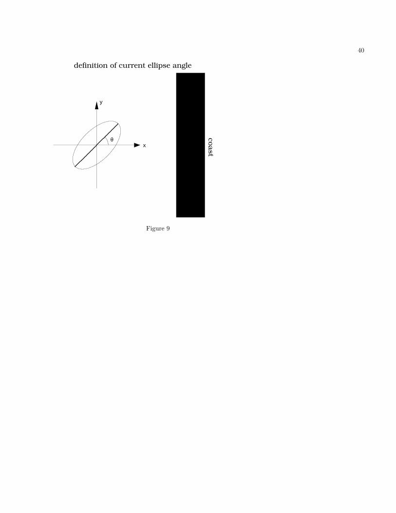
The orientation of the major axis of the current ellipseis the angle the major axis makes to the cross-shoredirection. The angle is constrained to be between -90◦

and 90◦ and is defined in Figure 9 as being positive inthe counterclockwise sense.

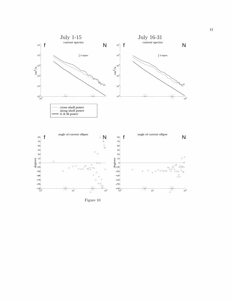
Figure 10 includes plots of the ellipse orientation forthe 55 m current meter at the C5 mooring. It illus-trates a surprisingly constant major axis angle over the6-40 cpd range of the analysis. The scatter of the an-gles in Figure 10 is smaller than in most other records,but none of the other records shows a trend in the el-lipse orientation with frequency. Since the observed an-gles show no consistent relation to frequency, they havebeen averaged over the usual range of frequencies. Theaverages are in Table 1. The significance estimate wasagain formed with a Monte Carlo technique, in which105 synthetic isotropic random time series were created,and ellipse orientations as a function of frequency wereformed as with the data. The mean angle was definedas the angle that is closest to all the angles in a leastsquared distance sense. Angular distance was definedas being between −π/2 and π/2 because ellipse angleis ambiguous to a π radian rotation. The standard de-viation of angles around this mean was found for eachsynthetic isotropic series, and a distribution of thesestandard deviations was found. The standard devia-tion of the angles in the data was then compared tothe distributions of the synthetic data. All but one ofthe current meter records have angles whose distribu-tions are significantly (>95% confidence) different froman isotropic wave field. This again shows that the wavefield must be considered anisotropic

Several conclusions can be drawn from the angles inTable 1. Thirty-one of 32 averaged angles are negative,and many are near the -17◦ value consistent with bathy-metric steering and, thus are consistent with linear in-ternal wave energy propagating to the shore. (The shelfbreak is rotated relative to the shore by -17◦.) The an-gles at C4 are more negative when the bottom half of thewater column flows to the equator, as the Doppler shifttheory in PB would predict. Conversely, the angles at

13

C5 are less negative when the currents are flowing equa-torward. This is puzzling, for it is not what PB wouldpredict, and the difference is in the sign of the effect,not just the magnitude. Perhaps some alongshore vari-ability in the currents is focusing internal waves. The 20m current meter at C4 has current ellipses with anglesof ≈ -60◦ to the cross-shelf direction with very littlescatter with frequency. This anomalous result could becaused by the broken current meter blades found on oneof the rotors upon recovery of the mooring.

7. Modal Decomposition

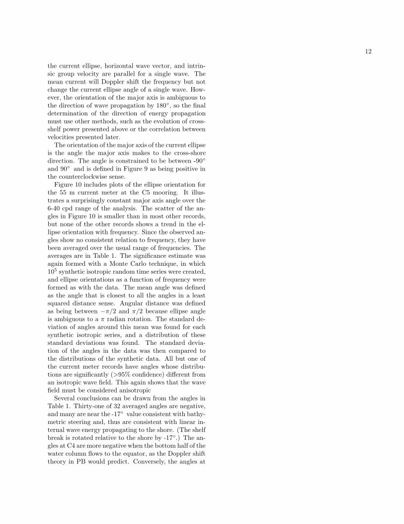
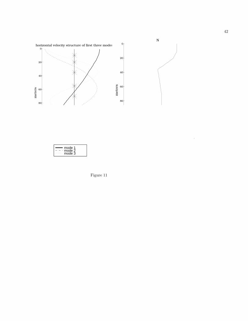
From a modal decomposition of the data, the direc-tion of wave propagation can be found, the verticalstructure of the waves can be found and more detailedcomparisons can be made to the PB theory. The powerin the horizontal and vertical currents can also be shownto be consistent with linearized internal waves. Unfor-tunately, decomposition into vertical modes can onlybe done at C4, for the current meters at C5 are badlyspaced for a decomposition, and the hourly data at theshallower site make it difficult to compute robust statis-tics. The details of the decomposition have been left tothe appendix, but a summary follows. Using the meanbuoyancy profile for the month (Figure 11), the vertical Figure 11modal structures are calculated for a frequency of 10cpd, so f2 � ω2 � N2. These modes, also illustratedin Figure 11, are shown in PB not to vary substantiallywith frequency for frequencies greater than the criticalfrequency of reflection and lower than the buoyancy fre-quency. It is these restrictions that define the 6 to 40cpd frequency range to which the gathering of statisticsis confined. The modes are fit at each time step to thecurrent meter data, with u, v, and w fit independently.The fit is optimal in a least squares sense. The verti-cal velocity w is determined from the time derivative oftemperature and the vertical gradients of temperature.

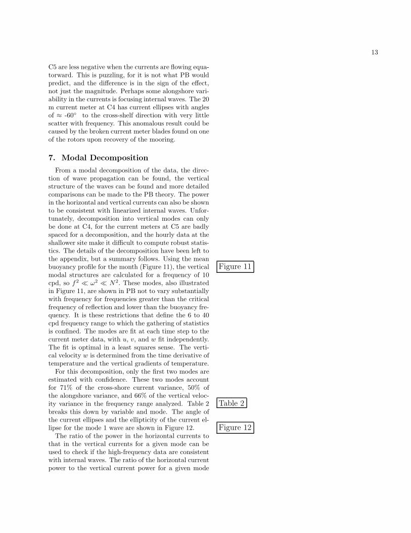
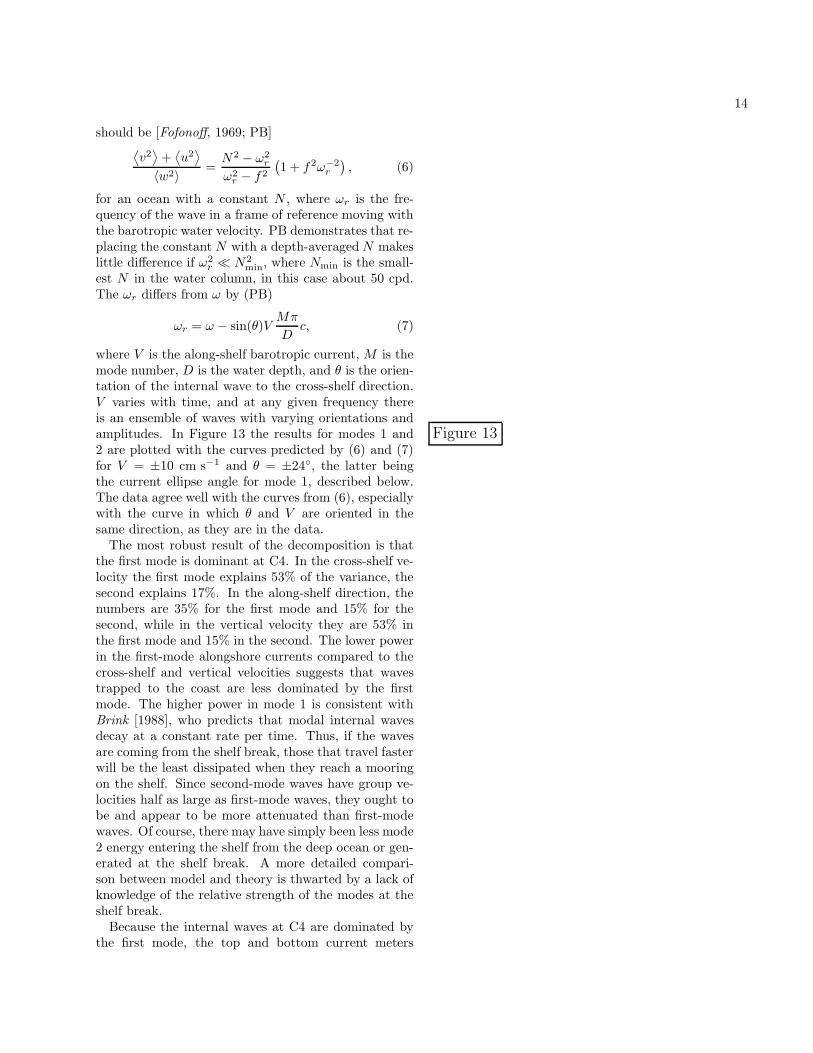
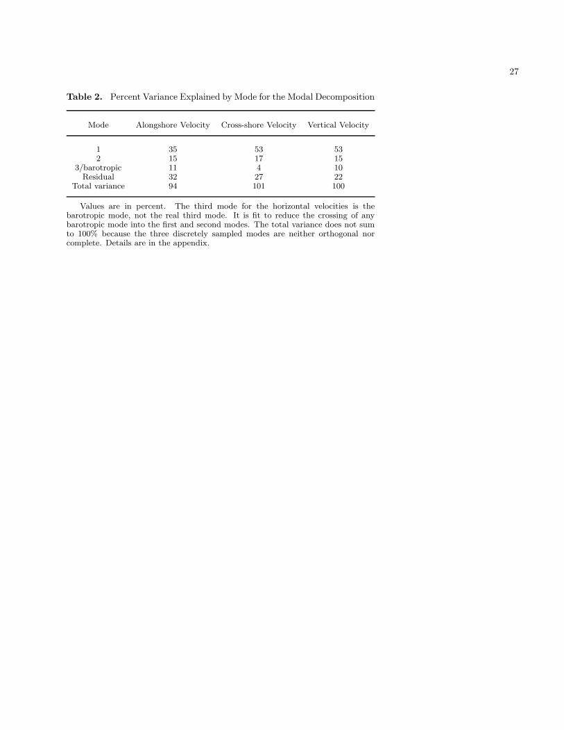
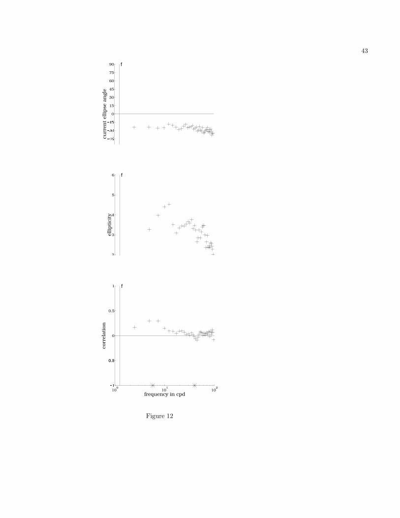
For this decomposition, only the first two modes areestimated with confidence. These two modes accountfor 71% of the cross-shore current variance, 50% ofthe alongshore variance, and 66% of the vertical veloc-ity variance in the frequency range analyzed. Table 2 Table 2breaks this down by variable and mode. The angle ofthe current ellipses and the ellipticity of the current el-lipse for the mode 1 wave are shown in Figure 12. Figure 12

The ratio of the power in the horizontal currents tothat in the vertical currents for a given mode can beused to check if the high-frequency data are consistentwith internal waves. The ratio of the horizontal currentpower to the vertical current power for a given mode

14

should be [Fofonoff, 1969; PB]⟨v2⟩

+⟨u2⟩

〈w2〉 =N2 − ω2

r

ω2r − f2

(1 + f2ω−2

r

), (6)

for an ocean with a constant N , where ωr is the fre-quency of the wave in a frame of reference moving withthe barotropic water velocity. PB demonstrates that re-placing the constant N with a depth-averaged N makeslittle difference if ω2

r � N2min, where Nmin is the small-

est N in the water column, in this case about 50 cpd.The ωr differs from ω by (PB)

ωr = ω − sin(θ)VMπ

Dc, (7)

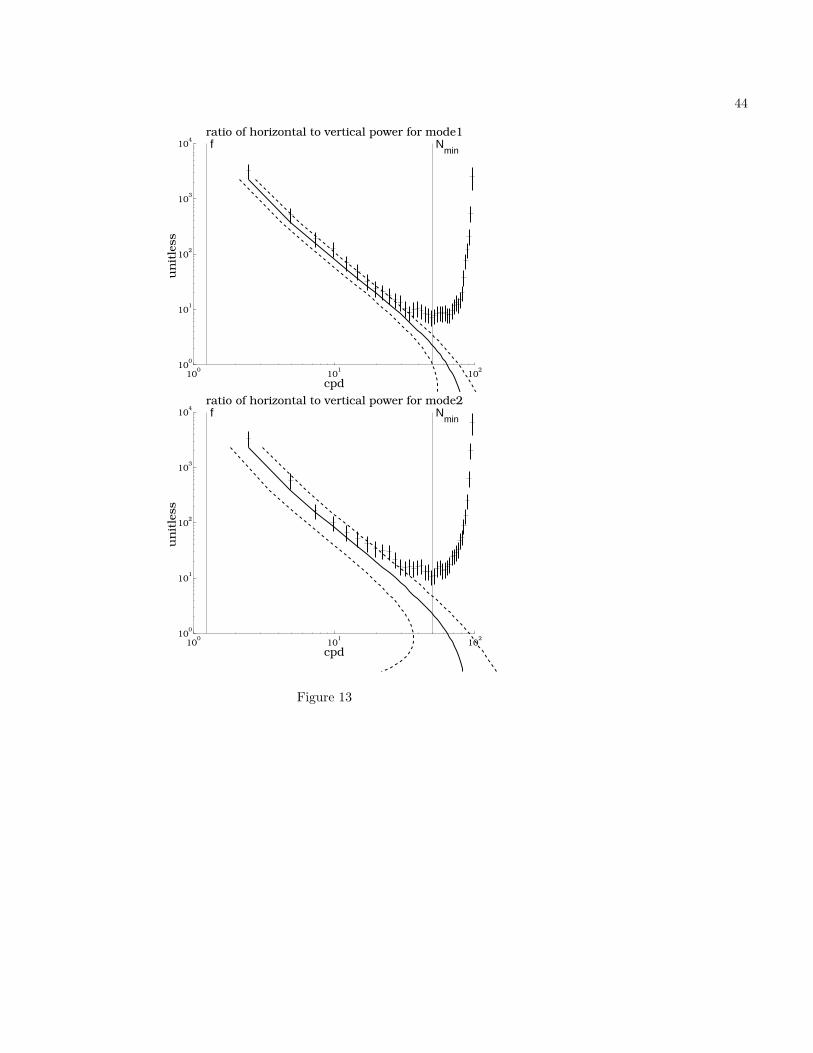
where V is the along-shelf barotropic current, M is themode number, D is the water depth, and θ is the orien-tation of the internal wave to the cross-shelf direction.V varies with time, and at any given frequency thereis an ensemble of waves with varying orientations andamplitudes. In Figure 13 the results for modes 1 and Figure 132 are plotted with the curves predicted by (6) and (7)for V = ±10 cm s−1 and θ = ±24◦, the latter beingthe current ellipse angle for mode 1, described below.The data agree well with the curves from (6), especiallywith the curve in which θ and V are oriented in thesame direction, as they are in the data.

The most robust result of the decomposition is thatthe first mode is dominant at C4. In the cross-shelf ve-locity the first mode explains 53% of the variance, thesecond explains 17%. In the along-shelf direction, thenumbers are 35% for the first mode and 15% for thesecond, while in the vertical velocity they are 53% inthe first mode and 15% in the second. The lower powerin the first-mode alongshore currents compared to thecross-shelf and vertical velocities suggests that wavestrapped to the coast are less dominated by the firstmode. The higher power in mode 1 is consistent withBrink [1988], who predicts that modal internal wavesdecay at a constant rate per time. Thus, if the wavesare coming from the shelf break, those that travel fasterwill be the least dissipated when they reach a mooringon the shelf. Since second-mode waves have group ve-locities half as large as first-mode waves, they ought tobe and appear to be more attenuated than first-modewaves. Of course, there may have simply been less mode2 energy entering the shelf from the deep ocean or gen-erated at the shelf break. A more detailed compari-son between model and theory is thwarted by a lack ofknowledge of the relative strength of the modes at theshelf break.

Because the internal waves at C4 are dominated bythe first mode, the top and bottom current meters

15

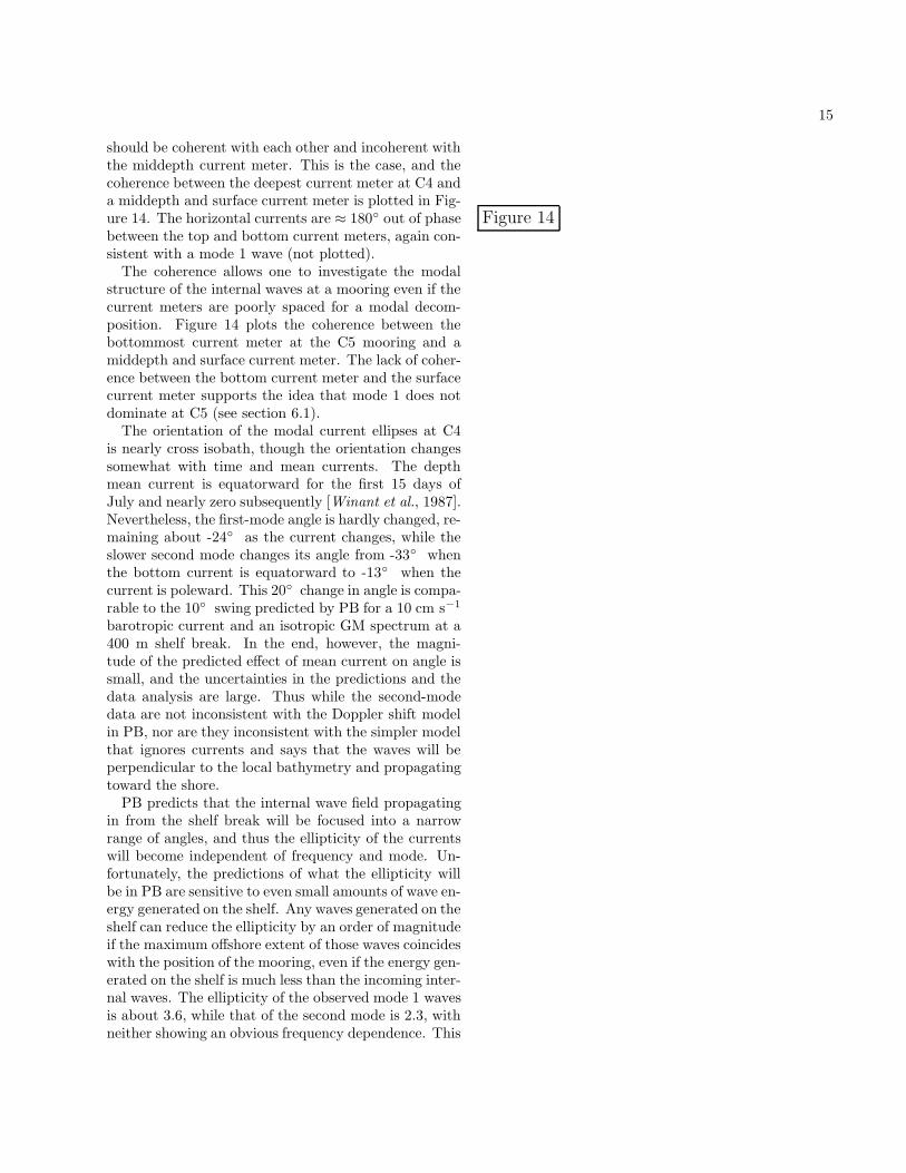
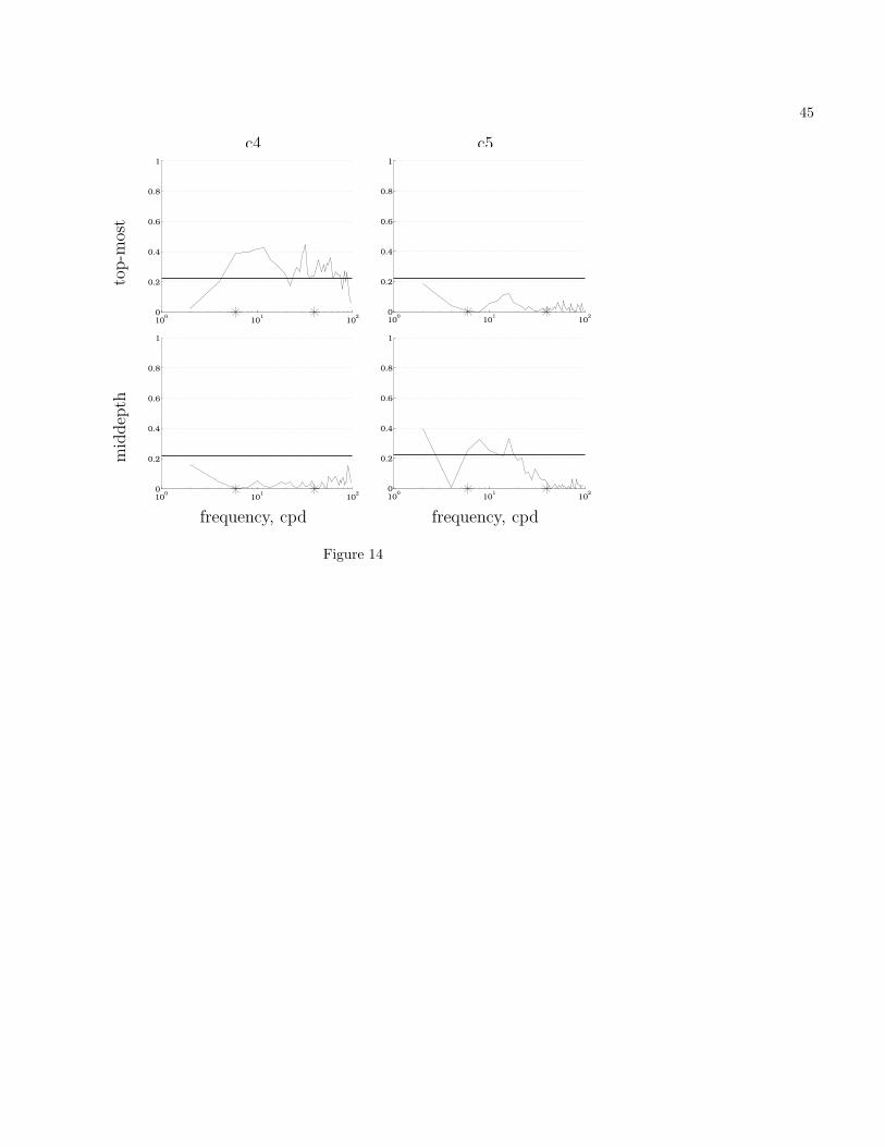
should be coherent with each other and incoherent withthe middepth current meter. This is the case, and thecoherence between the deepest current meter at C4 anda middepth and surface current meter is plotted in Fig-ure 14. The horizontal currents are ≈ 180◦ out of phase Figure 14between the top and bottom current meters, again con-sistent with a mode 1 wave (not plotted).

The coherence allows one to investigate the modalstructure of the internal waves at a mooring even if thecurrent meters are poorly spaced for a modal decom-position. Figure 14 plots the coherence between thebottommost current meter at the C5 mooring and amiddepth and surface current meter. The lack of coher-ence between the bottom current meter and the surfacecurrent meter supports the idea that mode 1 does notdominate at C5 (see section 6.1).

The orientation of the modal current ellipses at C4is nearly cross isobath, though the orientation changessomewhat with time and mean currents. The depthmean current is equatorward for the first 15 days ofJuly and nearly zero subsequently [Winant et al., 1987].Nevertheless, the first-mode angle is hardly changed, re-maining about -24◦ as the current changes, while theslower second mode changes its angle from -33◦ whenthe bottom current is equatorward to -13◦ when thecurrent is poleward. This 20◦ change in angle is compa-rable to the 10◦ swing predicted by PB for a 10 cm s−1

barotropic current and an isotropic GM spectrum at a400 m shelf break. In the end, however, the magni-tude of the predicted effect of mean current on angle issmall, and the uncertainties in the predictions and thedata analysis are large. Thus while the second-modedata are not inconsistent with the Doppler shift modelin PB, nor are they inconsistent with the simpler modelthat ignores currents and says that the waves will beperpendicular to the local bathymetry and propagatingtoward the shore.

PB predicts that the internal wave field propagatingin from the shelf break will be focused into a narrowrange of angles, and thus the ellipticity of the currentswill become independent of frequency and mode. Un-fortunately, the predictions of what the ellipticity willbe in PB are sensitive to even small amounts of wave en-ergy generated on the shelf. Any waves generated on theshelf can reduce the ellipticity by an order of magnitudeif the maximum offshore extent of those waves coincideswith the position of the mooring, even if the energy gen-erated on the shelf is much less than the incoming inter-nal waves. The ellipticity of the observed mode 1 wavesis about 3.6, while that of the second mode is 2.3, withneither showing an obvious frequency dependence. This

16

suggests there is relatively more alongshore propagat-ing energy in the second mode than in the first. Also,for both modes the ellipticity increases in the secondhalf of the month, though only in the first mode is thisincrease significant, from 3.29 to 4.34. This suggestsa decrease in alongshore energy in the second part ofthe month. The tentativeness of this analysis indicatesthe difficulty of understanding the internal wave fieldwithout some measure of the horizontal wave numberspectrum.

The modal data can help to determine the directionof internal wave propagation. To do this, it is necessaryto define the “spectral correlation coefficient.” This isthe normalized cospectrum of two time series at a givenfrequency, defined as

〈vw〉 =Covw√PvvPww

, (8)

where Covw is the cospectrum of v and w and Pvv andPww are the power at a given frequency in v and w,respectively. The structure of an internal wave propa-gating in the x direction is, when represented modally,

u = −1

k

dW

dzsin (kx− ωt+ φ) , (9a)

v =f

kω

dW

dzcos (kx− ωt+ φ) , (9b)

w = W (z) cos (kx− ωt+ φ) , (9c)

where k is the wave number, ω is the angular frequency,and φ is a phase (PB). From (9a)-(9c) it is easy to seethat for a single plane wave traveling in the positive xdirection, the correlation 〈vw〉 is 1 and the major axisof the internal wave is oriented along the x axis. Thus,for a single wave, once the angle of the major axis ofthe current ellipse has been determined for a given fre-quency, the mean direction of wave propagation alongthe major axis can be determined from the sign of thecorrelation of the vertical velocity and the current inthe minor axis direction. Unfortunately, for a set of in-ternal waves propagating onto the coast with a range ofangles, the computation of the correlation is more com-plicated. As a simplified version the model in PB, thecorrelation is calculated assuming waves of equal am-plitude and random phase propagating at angles from-θc to θc around the major axis. Computing the theo-retical correlation of the minor axis velocities and thevertical velocities for modally decomposed waves of ran-dom phase and constant amplitude, one obtains

〈vw〉 =2fω sin(θc)√

2θc

(1 + f2

ω2

)+ θc sin (2θc)

(f2

ω2 − 1) , (10)

17

where θc is computed in PB as a function of δ, the ratioof the water depth at the observation site to the depthwhere an internal wave first “feels” the bottom:

θc = arctan

(1√

δ−1 − 1

). (11)

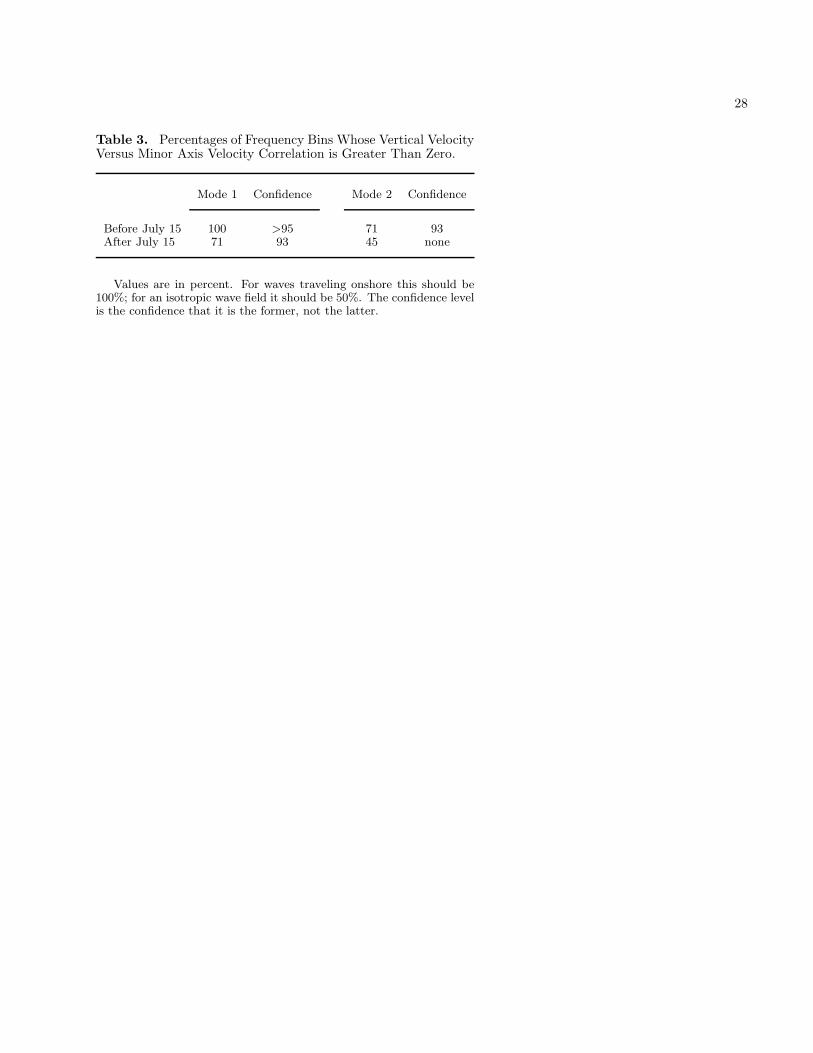
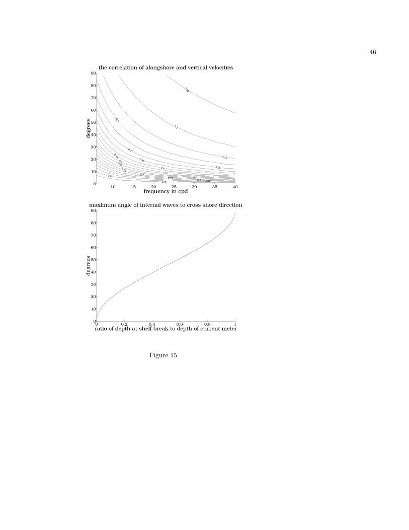
θc is shown as a function of δ and 〈vw〉 is shown as afunction of θc in Figure 15. Assuming δ ≈ 0.3 to 0.4 Figure 15for the 130 m site, the correlation should lie between 0.1and 0.4. Correlations of 0.1 to 0.4 for a single frequencyare hard to distinguish from white noise. However, itbecomes possible to test for propagation onshore if thetest is whether the correlation is positive. This testdistinguishes waves going onshore from a random wavefield, whose correlation would be randomly distributedaround zero, and also from waves propagating offshore.It cannot test between various models of the distribu-tion of energy with angle. The test is made by rotatingthe data at each frequency so that u is in the directionof the major axis that points onshore and v is parallelto the minor axis, which makes the coordinate systemright-handed. Then the correlation 〈vw〉 is formed andplotted in Figure 12. Table 3 gives the percentage of Table 3frequencies whose correlation is positive and the con-fidence that this percentage is distinguishable from anisotropic internal wave field. Since u is rotated so thatthe onshore component of a positive u is positive, when〈vw〉 is positive, the waves are propagating onshore. Allof the mode 1 data are consistent with onshore prop-agation at a better than 93% level, while the mode 2data are only consistent with onshore propagation be-fore July 15. The mode 2 correlations after July 15 areindistinguishable from white noise.

There are some caveats to this method. The cor-relation is very sensitive to the range of angles overwhich the waves are propagating. Thus, if an ensembleof waves propagated onshore at a range of angles from-10◦ to 10◦ and the same amount of energy went off-shore spread between -30◦ and 30◦, this method wouldindicate that energy was propagating into the shore.These are the limitations of not measuring the wavenumber spectrum directly.

8. Variation in Power With Space andTime

Inherent in the GM spectrum is an assumption thatthe energy levels of the internal wave spectrum are con-stant with time. This is not true for the internal waveson the shelf in the CODE region. The determinationthat the energy levels are not stationary is tricky, forany finite-length moving average of a truly random time

18

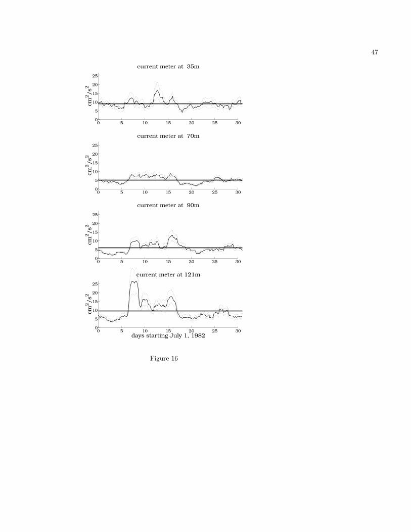
series will fluctuate. These fluctuations are larger for ared spectrum. Figure 16 is a plot of a 2 day moving Figure 16average of the power over the 6 to 40 cpd frequencyband from the 35, 70, 90, and 121 m current metersat C4, along with 1 standard deviation error bars com-puted from the periodograms. The error bars accountfor the redness of the spectrum. The mean energy is alsoplotted. The standard deviations of the data are smallenough and the degrees of freedom large enough, thatthe chi-square distributions can be considered Gaussian.The observations from 35 m were more than 1 standarddeviation from the monthlong mean 32% of the time,at 70 m for 68% of the time, at 90 m for 67% of thetime, and at 121 m for 80% of the time. For a station-ary Gaussian-distributed time series, this should onlybe true 34% of the time, indicating that the power lev-els are not stationary. The variations of the power fromthe mean power are not more than a factor of 2.5. Verysimilar results hold for an analysis done over the monthsof June, July, and August, though the uncertainty inthe interpretation increases with the uncertainty in thebackground stratification over this longer time period.

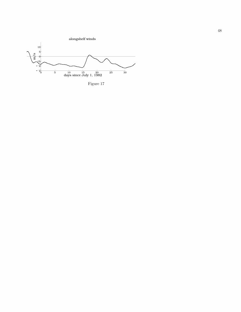
Neither the fluctuations in N plotted in Figure 4 northe fluctuations in the along-shelf wind in Figure 17 Figure 17show any correlation with the power fluctuations. Thisis also true for the time series of N at the other depths,the time series of winds at other nearby locations, andthe time series of alongshore current and current shear.Perhaps the fluctuations in internal wave power are theresults of the focusing of internal waves by alongshorevariations in the current field.

9. Discussion and Conclusion

The observations can be summarized by contrastingthose results that are consistent with internal wave en-ergy existing in the deep ocean as a GM spectrum andpropagating onto the shelf and those results that sug-gest that waves must also be generated, or at leastseverely modified from the predictions of a linear theory,on the shelf or at the shelf break.

The decline of total energy levels approaching theshore strongly supports the model of waves originatingin deep water or at the shelf break and being erodedby friction as they propagate onshore. In a scenariowith no friction or any scenario for generation of out-ward propagating waves near the shore, the energy lev-els would be expected to increase near the coast.

The orientation and ellipticity of the current ellipsesare consistent with an ensemble of internal waves prop-agating in from the deep ocean, though the failure ofthe ellipticity to increase shoreward (as predicted by

19

PB) suggests that waves generated on the shelf are alsopropagating onshore, thus broadening the angular dis-tribution of the waves. Propagation toward the coast isalso supported by the sign of the correlation of the ver-tical and minor axis velocities of modes 1 and 2 waves.

The dominance of mode 1 waves at the C4 site isagain consistent with the frictional model in PB, sincemode 1 waves are the least affected by friction. Thisargument cannot be made more convincing, however,without better knowledge of how deep water modes pen-etrate onto the shelf. It seems that mode 1 does notdominate at C5.

There are facts that conflict with the picture in PBand indicate that while a GM spectrum propagating infrom the deep ocean or shelf break is probably the dom-inant source of internal waves on the shelf, it is certainlynot the only one. It may be that a significant portionof the internal wave energy on the shelf is generated onthe shelf. It may also be that the theory is too naivein its linearity, in its simple assumption that the along-shore current is barotropic, or in its assumption of noalongshore variability in topography on frequency.

The most puzzling finding is that the spectrum be-comes less red closer to shore. The slower high-frequencywaves should be dissipated more rapidly than the low-frequency waves. The observed bluing of the spectrummeans that either energy is being generated preferen-tially at higher frequencies on the shelf or that nonlin-ear interactions are shifting the energy in the spectrumto the higher frequencies.

Thus the most plausible qualitative synthesis of ob-servations is of a GM spectrum propagating onto theshelf accompanied by shoreward propagating waves gen-erated on the shelf. In order to clarify this possibility,it would be necessary to have observations of the modalstructure of the waves at several different locations andideally some knowledge of the directional spectrum ofthe waves.

It is also worth observing that on continental shelvesbroader than at the CODE region, PB indicates that itis likely that dissipation would eliminate all waves fromthe deep ocean before the shore is reached, which wouldconsiderably alter the internal wave climate.

Appendix

In a flat bottom ocean the internal wave spectrumcan be broken into vertical modes that are orthogonalto each other [LeBlond and Mysak, 1978]. Given u andv as horizontal velocities and w as the vertical velocity,

20

the linearized system of equations on an f plane is

∂u

∂t− fv = − 1

ρ0

∂P

∂x, (A1a)

∂v

∂t+ fu = − 1

ρ0

∂P

∂y, (A1b)

∂w

∂t= − 1

ρ0

∂P

∂z− ρg

ρ0, (A1c)

∂u

∂x+∂v

∂y+∂w

∂z= 0, (A1d)

∂ρ

∂t− ρ0

gN2(z)w = 0. (A1e)

This system admits internal wave solutions of the form

u = −1

k

dW

dzsin (kx− ωt+ φ) , (A2a)

v =f

kω

dW

dzcos (kx− ωt+ φ) , (A2b)

w = W (z) cos (kx− ωt+ φ) , (A2c)

where φ is a phase, k is the horizontal wave number, ωis the angular frequency, and W (z) is the vertical modalstructure. W (z) is determined by

d2W

dz2+ k2

(N2(z)− ω2

ω2 − f2

)W = 0 (A3)

with W = 0 at the surface and bottom. If N is constant,W has the form

W = sin

(Mπ

Dz

)M = 0...∞. (A4)

If N depends on depth, the structure of the mode isno longer independent of ω2. However, as shown inPB, if N2 � ω2, as is true of this analysis, the modalstructure is independent of ω2 to a very good approx-imation. Thus the modal decomposition will be donefor the ω = 10 cpd modes. The results are insensitiveto the choice of ω.

This analysis is only true for a flat bottom, however,since the boundary condition is W = 0 at the bottom.However, Wunsch [1969] showed that the vertical modalsolution is approximately valid for waves whose frequen-cies are much less than the frequency of critical reflec-tion, which is true for this analysis. This approximationis justified in greater detail in PB.

The actual decomposition of the data was done on thehorizontal and vertical velocities. The vertical velocitieswere estimated by assuming the temperature balance

Tt + wTz = 0 (A5)

21

and computing Tz from low-pass filtered current meterdata. The modal functions were computed for the meanhydrography. This is less critical than it may appear,for the low modes are not very sensitive to changes inN . The amplitude of each mode was found by fittingthe computed modes to the current meter data at eachtime record, fitting u, v, and “w” independently. Thedata were depth weighted, but this made little differencebecause the current meters were nearly evenly spaced.The fit was optimal in a least squares sense.

This straightforward method obscures several sub-tle issues in the decomposition. The first problemis that while the internal wave modes are orthogo-nal, a set of discrete measurements in the water col-umn are not, in general, orthogonal. Unfortunately,to speak meaningfully of power in a mode, that modemust be orthogonal to all others. In order that all ofthe modes that are fit are nearly orthogonal to eachother (in the sense that for two modes W1 and W2,W1·W2/

√(W1 ·W1)(W2 ·W2)� 1, where W1·W2

is the inner product of W1 and W2 evaluated at themeasurement points), only five modes can be fit to theseven current meters. The fit is judged successful be-cause the sum of the power in each mode and the resid-ual (as shown in Table 2) is never more than 6% differ-ent from the total power. If the data from the top twocurrent meters are discarded, the power in the modesexplains 180% of the variance, with most of the dupli-cation of power being in the lowest two modes. Thusdiscarding the top two current meters is untenable.

It is unfortunate that the need for orthogonalityforces one to use the top two current meters, since theyare on a different mooring. This mooring is describedas nominally being 100 m to the northwest of the sub-surface mooring and was certainly not more than 200m away [Beardsley et al., 1985, and S. J. Lentz, per-sonal communication 1997]. The horizontal decorrela-tion length scale for horizontal currents will be half awavelength for waves with a finite beam width.

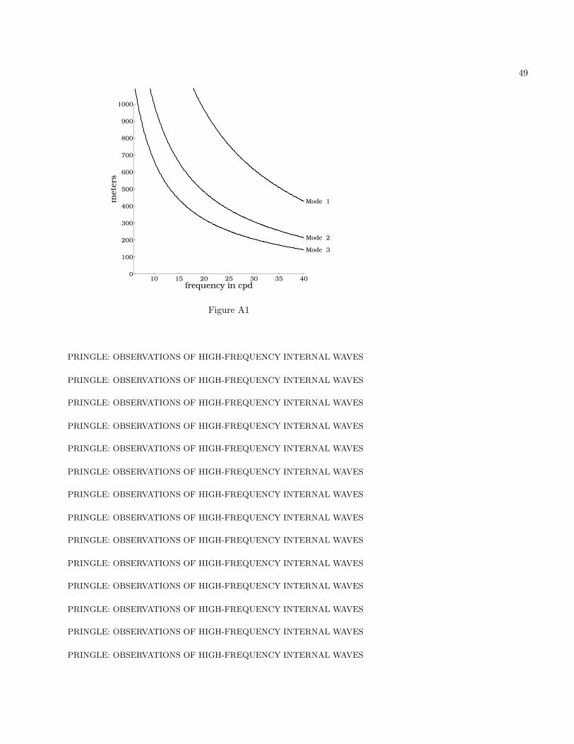
Figure A1 is a plot of the wavelengths of the first five Figure A1modes as a function of frequency. From this it can beseen that if the separation between the first two moor-ings is 100 m, mode 2 becomes nearly decorrelated at 40cycles per day. In the worst case, with a separation of200 m, the second mode becomes decorrelated at about23 cycles per day.

The amount of power in a real mode that is spuriouslytransferred to another mode because of any decorrela-tion of the top 2 m from the lower current meters canbe calculated. This calculation shows that, at the worstcase of 200 m separation, 20% of mode 1 horizontal cur-

22

rent power will leak into mode 2, while 20% of the hor-izontal current power in mode 2 can leak into mode 1.However, only 5% percent of the vertical current powerin mode 2 can leak into mode 1 vertical current powerand vice versa. Little mode 1 and 2 power would beleaked to the higher modes. The vertical power is 53%in the first mode and 15% in the second mode, and thecross-shore power is 53% in the first mode and 17% inthe second (Table 2). This partition remains true forfrequencies in the 25-40 cpd range. If the two moor-ings were so far apart that mode 1 would decorrelate,the cross-shore mode 2 power would be greater thanthe vertical mode 2 power, since more of the horizontalmode 1 power would leak into horizontal mode 2 thanvertical mode 1 power into vertical mode 2. Likewise,if only mode 2 decorrelated, the fraction of cross-shorepower in mode 2 would be less than the fraction of ver-tical power in mode 2, since more mode 2 power wouldleak in the horizontal modes than vertical modes. Thusthe the moorings are probably 100 m or less apart.

Even with only 100 m between the two current me-ter moorings, it must be assumed that modes higherthan the second are decorrelated. Similar calculationsto the ones above show that it becomes impossible tosort out the energy in the higher but resolvable modesbut that the partition of about 30% of the energy tomodes higher than the second mode is robust.

The possibility of modes higher than the theoreticallyobservable fifth mode being aliased into the low modes isimpossible to rule out, but it seems improbable that it issignificant because the energy decreases monotonicallyfor the first five modes.

23

Acknowledgments. I would like to thank the peoplewho helped me get the data for this paper, especially Su-san Tarbell and Carol Alessi, both of whom helped me findthe current meter data and tutored me in the interpreta-tion of mooring logs. The data came from the CODE pro-grams, and so thanks go to all who collected the data andplanned the programs. This paper benefited greatly fromSteve Lentz’s close reading and would have been impossiblewithout Ken Brink’s many readings and numerous pieces ofscientific advice. The work was funded by an Office of NavalResearch fellowship and Office of Naval Research AASERTfellowship, N00014-95-1-0746. Woods Hole OceanographicInstitution contribution 9629.

24

References

Beardsley, R. C., and S. J. Lentz, The Coastal Ocean Dy-namics Experiment collection: An introduction, J.Geophys. Res., 92(C2), 1455–1463, 1987.

Beardsley, R. C., R. Limeburner, and L. K. Rosenfeld, In-troduction, in CODE-2: Moored Array and Large-Scale Data Report, Technical Report 85-35, WoodsHole Oceanogr. Inst., Woods Hole, Mass., Nov.1985.

Brink, K. H., On the effect of bottom friction on internalwaves, Cont. Shelf Res., 8(4), 397–403, 1988.

Fofonoff, N. P., Spectral characteristics of internal waves inthe ocean, Deep Sea Res., 16, 59–71, 1969.

Garrett, C., and W. Munk, Space-time scales of internalwaves, Geophys. Fluid Dyn., 3, 225–264, 1972.

Gordon, R. L., Internal wave climate near the coast of north-west Africa during JOINT-1, Deep Sea Res., 25,625–643, 1978.

Howell, T. L., and W. S. Brown, Nonlinear internal waves onthe california continental shelf, J. Geophys. Res.,90(C4), 7256–7264, 1985.

Huyer, A., J. Fleischbein, and R. Schramm, Hydrographicdata from the second coastal ocean dynamics ex-periment: R/V Wecoma, Leg 9, 6-27 July 1982,Data Report 109, Ref. 84-7, Coll. of Oceanogr.,Oregon State Univ., Corvallis, April, 1983.

Kosro, P. M., and A. Huyer, CTD and velocity surveys ofseaward jets off northern California, July 1981 and1982, J. Geophys. Res., 91(C6), 7680–7690, 1986.

Kunze, E., Near-inertial wave propagation in geostrophicshear, J. Phys. Oceanogr., 15, 544–565, 1985.

LeBlond, P. H., and L. A. Mysak, Waves in the Ocean, El-sevier Sci., New York, 1978.

Lighthill, J., Waves in Fluids, Cambridge Univ. Press, NewYork, 1978.

Lynch, J. F., G. Jin, R. Pawlowicz, D. Ray, C. -S. Chiu,J. H. Miller, R. H. Bourke, A. R. Parsons, and R.Muench, Acoustic travel-time perturbations due toshallow-water internal waves and internal tides inthe Barents Sea Polar Front: Theory and experi-ment, J. Acoust. Soc. of Am., 99(2), 289–297, 1996.

McKee, W. D., Internal-inertial waves in a fluid of variabledepth, Proc. Cambridge Philos. Soc., 73, 205–213,1973.

Pringle, J. M., and K. H. Brink, High Frequency Inter-nal Waves on a Sloping Shelf, J. Geophys. Res.,this issue.

Sandstrom, H., and J. A. Elliott, Internal tide and solitonson the scotian shelf: A nutrient pump at work, J.Geophys. Res., 89(C4), 6415–6426, 1984.

Sanford, L. P., and W. D. Grant, Dissipation of internalwave energy in the bottom noundary layer on thecontinental shelf, J. Geophys. Res., 92(C2), 1828–1844, 1987.

25

Winant, C. D., R. C. Beardsley, and R. E. Davis, Mooredwind, temperature, and current observations madeduring coastal ocean dynamics experiments 1 and2 over the northern california continental shelf andupper slope, J. Geophys. Res., 92(C2), 1569–1604,1987.

Wunsch, C., Geographical variability of the internal wavefeild: A search for sources and sinks, J. Phys. Oceanogr.,6, 471–485, 1976.

Wunsch, C., On the propagation of internal waves up a slope,Deep Sea Res., 15, 251–258, 1968.

Wunsch, C., Progressive internal waves on slopes, J. FluidMech., 35, 131–144, 1969.

James Pringle, Scripps Institution of Oceanography, Uni-verisity of California, San Diego, Mail Stop 0218, La Jolla,CA 92093-0218 (email: [email protected])

(Received July 18, 1997; revised July 28, 1998;accepted August 14, 1998.)

1Now at Scripps Institution of Oceanography, Universityof California, San Diego, La Jolla.

Copyright 1999 by the American Geophysical Union.

Paper number 1998JC900053.0148-0227/98/1998JC900053$09.00

(Received July 18, 1997; revised July 28, 1998;accepted August 14, 1998.)

Copyright 1999 by the American Geophysical Union.

Paper number 1998JC900053.

0148-0227/98/1998JC900053$09.00

26

Table 1. Angle That the Average Current Ellipse Makes With the Cross-Shore Direction and the Ellipticity of the Current Ellipse for the C4 and C5Moorings for the 2 Week Periods Before and After July 15, 1982

Before July 15 After July 15

Depth, m Mean Angle, deg Ellipticity Mean Angle,deg Ellipticity

C4 Mooring

10 -36±6 2.49±0.37 -23±5 2.79±0.4220 -72±7 1.83±0.39 -49±4 2.83±0.2835 -16±53∗ 1.35±0.21∗ -49±21 1.60±0.4055 -22±9 1.64±0.25 -17±18 1.53±0.2370 -20±15 1.83±0.38 -2±9 1.95±0.3690 -12±16 1.53±0.25 4±9 2.03±0.35121 -16±5 4.41±1.17 -16±4 5.02±0.80

C5 Mooring

20 -4±27 1.34±0.16∗ -15±15 1.91±0.3435 -8±24 1.37±0.22 -10±10 2.00±0.5455 -17±5 1.79±0.31 -26±5 2.35±0.3870 -9±9 2.27±0.47 -13±3 2.42±0.3990 -13±11 1.93±0.27 -9±6 2.49±0.31110 -20±7 2.31±0.43 -22±7 3.21±0.62150 -12±6 2.81±0.69 -20±10 2.06±0.63250 -26±37 1.53±0.33 -34±21 1.47±0.31350 -14±7 2.73±0.79 -22±8 2.62±0.68

The averages are made by calculating the ellipticity and angle at each frequencyin the 6 to 40 cpd frequency range and then averaging the results with an evenweighting. The deviations are standard deviation, not the standard error.

Stars mark ellipticity or angles not significantly different from white noise at the95% confidence level, using the tests described in the text.

27

Table 2. Percent Variance Explained by Mode for the Modal Decomposition

Mode Alongshore Velocity Cross-shore Velocity Vertical Velocity

1 35 53 532 15 17 15

3/barotropic 11 4 10Residual 32 27 22

Total variance 94 101 100

Values are in percent. The third mode for the horizontal velocities is thebarotropic mode, not the real third mode. It is fit to reduce the crossing of anybarotropic mode into the first and second modes. The total variance does not sumto 100% because the three discretely sampled modes are neither orthogonal norcomplete. Details are in the appendix.

28

Table 3. Percentages of Frequency Bins Whose Vertical VelocityVersus Minor Axis Velocity Correlation is Greater Than Zero.

Mode 1 Confidence Mode 2 Confidence

Before July 15 100 >95 71 93After July 15 71 93 45 none

Values are in percent. For waves traveling onshore this should be100%; for an isotropic wave field it should be 50%. The confidence levelis the confidence that it is the former, not the latter.

29

Figure 1. The Coastal Ocean Dynamics Experiment(CODE) region, showing the central line of mooringsfrom the CODE II experiment. The C5, C4, and C3moorings are used herein.

Figure 1. The Coastal Ocean Dynamics Experiment (CODE) region, showing the central lineof moorings from the CODE II experiment. The C5, C4, and C3 moorings are used herein.

Figure 2. (top) Hydrography for the CODE region forthe April-July upwelling regime and (bottom) standarddeviations.

Figure 2. (top) Hydrography for the CODE region for the April-July upwelling regime and(bottom) standard deviations.

Figure 3. Average buoyancy frequency found fromconductivity-temperature-depth (CTD) casts on theshelf and shelf break in July 1982. The thick line isthe value computed with a full equation of state, whilethe thin line uses the empirical relation between tem-perature and potential density given by (5). The datahave been smoothed by a 10 m boxcar average.

Figure 3. Average buoyancy frequency found from conductivity-temperature-depth (CTD)casts on the shelf and shelf break in July 1982. The thick line is the value computed with afull equation of state, while the thin line uses the empirical relation between temperature andpotential density given by (5). The data have been smoothed by a 10 m boxcar average.

Figure 4. Buoyancy frequency of water between 55and 70 m at C4 as a function of time. The data werelow-pass filtered with a filter that had a half-amplitudepass at 3.25 times the inertial period (f=1.24 cpd) anda full pass at 4 times the inertial period.

Figure 4. Buoyancy frequency of water between 55 and 70 m at C4 as a function of time. Thedata were low-pass filtered with a filter that had a half-amplitude pass at 3.25 times the inertialperiod (f=1.24 cpd) and a full pass at 4 times the inertial period.

Figure 5. Low-pass-filtered alongshore currents at(top to bottom) 35 m depth at C3; 20 m depth at C4;90 m depth at C4; and 110 m depth at C5. The samelow-pass filter was used as in Figure 4.

Figure 5. Low-pass-filtered alongshore currents at (top to bottom) 35 m depth at C3; 20 mdepth at C4; 90 m depth at C4; and 110 m depth at C5. The same low-pass filter was used as inFigure 4.

Figure 6. Power spectra of cross- and along-shelf ve-locity for current meters (top) C5 at 90 m depth, (mid-dle) C4, 90 m depth, and (bottom) C3, 70 m depth.The thin solid line is the cross-shore power, the dashedline is the alongshore power, and the thick solid line isthe Garrett and Munk [1972] power. The stars on thefrequency axis mark the limits of the frequency rangeanalyzed. The power is in cm2 s−1, frequency is in cy-cles per day.

30

Figure 6. Power spectra of cross- and along-shelf velocity for current meters (top) C5 at 90m depth, (middle) C4, 90 m depth, and (bottom) C3, 70 m depth. The thin solid line is thecross-shore power, the dashed line is the alongshore power, and the thick solid line is the Garrettand Munk [1972] power. The stars on the frequency axis mark the limits of the frequency rangeanalyzed. The power is in cm2 s−1, frequency is in cycles per day.

Figure 7. Power in the 6 - 40 cpd frequency bandnormalized by the Garrett and Munk [1972] spectrumfor (top) C5 and (bottom) C4 moorings.

Figure 7. Power in the 6 - 40 cpd frequency band normalized by the Garrett and Munk [1972]spectrum for (top) C5 and (bottom) C4 moorings.

Figure 8. Slope of the power spectrum of each currentmeter in log-log space from (top) C5 and (bottom) C4.

Figure 8. Slope of the power spectrum of each current meter in log-log space from (top) C5and (bottom) C4.

Figure 9. Major axis of the illustrated current ellipse(thick line), and the angle of the major axis to the cross-shore direction θ, which is positive as drawn.

Figure 9. Major axis of the illustrated current ellipse (thick line), and the angle of the majoraxis to the cross-shore direction θ, which is positive as drawn.

Figure 10. (top) Power spectra and (bottom) the an-gle that the major axis of the current meter makes withthe cross-shelf direction for the (left) first and (right)last half of July for the current meter in 55 m of wa-ter at the C5 mooring. The arrows on the bottom axismark the frequency limits of the analysis.

Figure 10. (top) Power spectra and (bottom) the angle that the major axis of the currentmeter makes with the cross-shelf direction for the (left) first and (right) last half of July for thecurrent meter in 55 m of water at the C5 mooring. The arrows on the bottom axis mark thefrequency limits of the analysis.

Figure 11. (left) Horizontal velocity structure ofthe first three modes and (right) buoyancy frequencyprofile. The stars on the vertical axis mark the positionof the current meters at C4.

Figure 11. (left) Horizontal velocity structure of the first three modes and (right) buoyancyfrequency profile. The stars on the vertical axis mark the position of the current meters at C4.

Figure 12. (top) Angle of the current ellipses, (middle)ellipticity of the current ellipse, and (bottom) correla-tion between the currents parallel to the minor axis ofthe ellipse and the vertical velocity for mode 1. Thestars on the horizontal axis mark the frequency limit ofanalysis.

Figure 12. (top) Angle of the current ellipses, (middle) ellipticity of the current ellipse, and(bottom) correlation between the currents parallel to the minor axis of the ellipse and the verticalvelocity for mode 1. The stars on the horizontal axis mark the frequency limit of analysis.

31

Figure 13. Ratio of the horizontal and vertical cur-rent powers for (top) mode 1, and (bottom) mode 2.The solid line is the solution to (6) when the along-shelfbarotropic velocity V = 0 and/or the orientation of theinternal wave to the cross-shelf direction θ = 0, whilethe dashed lines are for V = ±10 cm s−1 and θ = ±24◦.The lower curve is for when the sign of V and θ differ,the upper curve is for when they are of the same sign.The error bars on the data are ± 1 standard deviation.

Figure 13. Ratio of the horizontal and vertical current powers for (top) mode 1, and (bottom)mode 2. The solid line is the solution to (6) when the along-shelf barotropic velocity V = 0and/or the orientation of the internal wave to the cross-shelf direction θ = 0, while the dashedlines are for V = ±10 cm s−1 and θ = ±24◦. The lower curve is for when the sign of V and θdiffer, the upper curve is for when they are of the same sign. The error bars on the data are ± 1standard deviation.

Figure 14. Coherence of cross-shelf current betweenthe bottommost current meter and the surface and mid-depth current meters for the C4 and C5 moorings. Thethick line is the 95% confidence level.

Figure 14. Coherence of cross-shelf current between the bottommost current meter and thesurface and middepth current meters for the C4 and C5 moorings. The thick line is the 95%confidence level.

Figure 15. (top) Correlation between the verticalvelocity and the horizontal velocity parallel to the mi-nor axis as a function of angular beam width and wavefrequency. (bottom) Beam width as a function of theratio of depth at which the waves feel the bottom to thedepth of the current meter.

Figure 15. (top) Correlation between the vertical velocity and the horizontal velocity parallelto the minor axis as a function of angular beam width and wave frequency. (bottom) Beam widthas a function of the ratio of depth at which the waves feel the bottom to the depth of the currentmeter.

Figure 16. The 2 day moving average of the powerfrom the (top to bottom) 20, 70, 90, and 121 m currentmeters at the 130 m site, along with 1 standard devia-tion error bars. The mean power is plotted as the thickhorizontal line.

Figure 16. The 2 day moving average of the power from the (top to bottom) 20, 70, 90, and121 m current meters at the 130 m site, along with 1 standard deviation error bars. The meanpower is plotted as the thick horizontal line.

Figure 17. The alongshelf winds at C4 for the monthof July. The winds have been low-pass filtered with thesame filter as used for Figures 4 and 5.

Figure 17. The alongshelf winds at C4 for the month of July. The winds have been low-passfiltered with the same filter as used for Figures 4 and 5.

Figure A1. Wavelengths of the first three internalwave modes in 130 m of water as a function of frequency;N = 77 cpd.

Figure A1. Wavelengths of the first three internal wave modes in 130 m of water as a functionof frequency; N = 77 cpd.

32

Please have AGU resize this figure

Figure 1

33

Please have AGU resize this figure

Figure 2

34

N from equation of state

N from T/sigma relation

0 50 100 150

0

50

100

150

200

250

300

350

400

dep

th in

met

ers

N in cpd

Average N profile

Figure 3

35

0 5 10 15 20 25 300

50

100

150

days since July 1, 1982

Average N between 55 and 70 meters at C4N

in

cpd

Figure 4

36

−20

0

20

cm/s

20 meters at C4

−20

0

20

cm/s

90 meters at C4

0 5 10 15 20 25 30

−20

0

20

days starting July 1, 1982 =0

cm/s

110 meters at C5

−20

0

20

35 meters at C3cm

/s

Figure 5

37

102

103

104

105

106

107

cm

2/s

2 sigma

f Nm2

90 meters at C5

102

103

104

105

106

107

cm

2/s

2 sigma

f Nm2

90 meters at C4

100

101

102

102

103

104

105

106

107

frequency in cpd

cm

2/s

2 sigma

f Nm2

70 meters at C3

cross shelf poweralong shelf powerG & M power

Figure 6

38

0 50 100 150 200 250 300 3500

0.5

1

1.5

2

2.5

3

3.5

4

4.5

5

C5 normalized by GM72 spectrum

nor

mal

ized

pow

er

depth in meters

0 50 100 150 200 250 300 3500

0.5

1

1.5

2

2.5

3

3.5

4

4.5

5

C4 normalized by GM72 spectrum

nor

mal

ized

pow

er

depth in meters

Figure 7

39

0 50 100 150 200 250 300 350−2.5

−2

−1.5

−1C5

Pow

er L

aw e

xpon

ent

depth in meters

��

alongshore powerlaw

0 50 100 150 200 250 300 350��

��

��

��C4

Pow

er L

aw e

xpon

ent

depth in meters

Figure 8

40

definition of current ellipse angle

x

y

θ coast

Figure 9

41

July 1-15 July 16-31

100

101

102

102

103

104

105

106

107

cm2/s

current spectra

2 sigma

f N

100

101

102

102

103

104

105

106

107

cm2/s

current spectra

2 sigma

f N

cross shelf poweralong shelf powerG & M power

100

101

102

� ��

��

��

��

��

��

0

15

30

45

60

75

90

deg

rees

angle of current ellipsef N

data/c

m

100

101

102

� ��

��

��

��

��

��

0

15

30

45

60

75

90

deg

rees

angle of current ellipsef N

data/c

m

Figure 10

42

� �� 0 0.1 0.2

0

20

40

60

80

100

120

horizontal velocity structure of first three modes

met

ers

�� 40 60 80 100 120

0

20

40

60

80

100

120

frequency in cpd

met

ers

N

mode 1mode 2mode 3

Figure 11

43

100

101

102

� ��

��

��

��

��

��

0

15

30

45

60

75

90

curr

ent

ellipse

an

gle

f

100

101

102

1

2

3

4

5

6

ellipti

city

f

100

101

102

��

��

0

0.5

1

frequency in cpd

corr

elat

ion

f

Figure 12

44

100

101

102

100

101

102

103

104

cpd

un

itle

ss

ratio of horizontal to vertical power for mode1 f N

min

100

101

102

100

101

102

103

104

cpd

un

itle

ss

ratio of horizontal to vertical power for mode2 f N

min

Figure 13

45

c4 c5

top-m

ost

100

101

102

0

0.2

0.4

0.6

0.8

1

100

101

102

0

0.2

0.4

0.6

0.8

1

mid

dep

th

100

101

102

0

0.2

0.4

0.6

0.8

1

100

101

102

0

0.2

0.4

0.6

0.8

1

frequency, cpd frequency, cpd

Figure 14

46

10 15 20 25 30 35 400

10

20

30

40

50

60

70

80

90

frequency in cpd

deg

rees

the correlation of alongshore and vertical velocities

0.05

0.1

0.15

0.2

0.25

0.3

0.35

0.4

0.45

0.50.55

0.6

0.65

0.70.75

0.8 0.85

0.9

0.95

0 0.2 0.4 0.6 0.8 10

10

20

30

40

50

60

70

80

90

ratio of depth at shelf break to depth of current meter

deg

rees

maximum angle of internal waves to cross shore direction

Figure 15

47

0 5 10 15 20 25 300

5

10

15

20

25

cm2/s2

current meter at 35m

0 5 10 15 20 25 300

5

10

15

20

25

cm2/s2


0 5 10 15 20 25 300

5

10

15

20

25

cm2/s2


0 5 10 15 20 25 300

5

10

15

20

25

cm2/s2


days starting July 1, 1982

Figure 16

48

0 5 10 15 20 25 30� ��

� ��

� �

0

5

10

alongshelf windsm

/s

days since July 1, 1982

Figure 17

49

10 15 20 25 30 35 400

100

200

300

400

500

600

700

800

900

1000

Mode 1

Mode 2

Mode 3

frequency in cpd

met

ers

Figure A1

PRINGLE: OBSERVATIONS OF HIGH-FREQUENCY INTERNAL WAVES














50


























51



























52



























53








Documents

Observations of high-frequency internal waves in …oxbow.sr.unh.edu/preprints/internalwaves_obs.pdf · Observations of high-frequency internal waves in the ... it can a ect diapycnal