San Jose State University San Jose State University

SJSU ScholarWorks SJSU ScholarWorks

Master's Theses Master's Theses and Graduate Research

Fall 2019

Observations of Fire Behavior on a Grass Slope During a Wind Observations of Fire Behavior on a Grass Slope During a Wind

Reversal Reversal

Dianne Hall San Jose State University

Follow this and additional works at: https://scholarworks.sjsu.edu/etd_theses

Recommended Citation Recommended Citation Hall, Dianne, "Observations of Fire Behavior on a Grass Slope During a Wind Reversal" (2019). Master's Theses. 5063. DOI: https://doi.org/10.31979/etd.9g2s-fd75 https://scholarworks.sjsu.edu/etd_theses/5063

This Thesis is brought to you for free and open access by the Master's Theses and Graduate Research at SJSU ScholarWorks. It has been accepted for inclusion in Master's Theses by an authorized administrator of SJSU ScholarWorks. For more information, please contact scholarworks@sjsu.edu.

OBSERVATIONS OF FIRE BEHAVIOR ON A GRASS SLOPE DURING A WIND REVERSAL

A Thesis

Presented to

The Faculty of the Department of Meteorology and Climate Science

San José State University

In Partial Fulfillment

of the Requirements for the Degree

Master of Science

by

Dianne Hall

December 2019

© 2019

Dianne Hall

ALL RIGHTS RESERVED

The Designated Thesis Committee Approves the Thesis Titled

OBSERVATIONS OF FIRE BEHAVIOR ON A GRASS SLOPE DURING A WIND REVERSAL

by

Dianne Hall

APPROVED FOR THE DEPARTMENT OF METEOROLOGY AND CLIMATE SCIENCE

SAN JOSÉ STATE UNIVERSITY

December 2019

Craig Clements, Ph.D. Department of Meteorology and Climate Science

Sen Chiao, Ph.D. Department of Meteorology and Climate Science

Alison Bridger, Ph.D. Department of Meteorology and Climate Science

ABSTRACT

OBSERVATIONS OF FIRE BEHAVIOR ON A GRASS SLOPE DURING A WIND REVERSAL

by Dianne Hall

This experiment studied fire-atmospheric interactions and wildland fire

behavior on a slope. A grass slope was instrumented with both in situ and

remote instruments to record both meteorological conditions and the fire

behavior. A headfire was lit and allowed to burn upslope through the

instruments. The data collected were analyzed to determine the fire behavior,

specifically fire spread (direction and rate) and flame characteristics (length,

height, and angle). During the first several minutes of the experiment, fire

behavior was as expected with an upslope rate of spread at 0.1 m s-1 and flame

lengths between 1 m and 4 m. However, the rest of the fire burned much more

slowly than expected with an upslope rate of spread of 0.02 m s-1 and flame

lengths of only between 0.25 m and 2 m. Backing fire behavior was observed.

Lidar analysis indicated that an upper level wind surfaced during the experiment

and a wind reversal occurred. During the initial part of the fire the wind was 45o

from upslope, so the wind and slope were mostly in alignment. During the

second part of the fire, the wind was downslope, so the wind and slope were in

opposition. From this experiment, we can conclude that the wind speed and

direction can overcome the influence of slope on fire behavior.

v

ACKNOWLEDGEMENTS

I would like to thank my Thesis Advisor, Dr. Craig Clements for exposing me

to the meteorological side of firefighting. I loved being a fire fighter and came to

understand fire behavior even more after joining the Fire Weather Research Lab.

Dr. Clements conceived of this experiment and I enjoyed working with the lab

members on this and several other fire experiments. Without the help and hard

work of the past and present members of the Fire Lab, this experiment would not

have occurred, and I am so grateful for the help and support. Fort Hunter Liggett

supplied the location for the experiment and went above and beyond in ensuring

our success.

I would like to thank my other Thesis Committee members, Dr. Sen Chiao

and Dr. Alison Bridger, for their guidance over the years with both their class

instruction and with this thesis. I have learned so much from you.

To my friends and family who supported over the years, I thank you, and

especially to Dr. Helen Mamarchev, without whose encouragement, this thesis

would not have been completed.

This research was made possible through a Fire Grant from National Institute

of Standards and Technology (NIST) 60NANB11D189, grants from the National

Science Foundation (NSF) Grants AGS-0960300, AGS-1151930 and the

International Association of Wildland Fire (IAWF) 2012 Graduate Scholarship.

vi

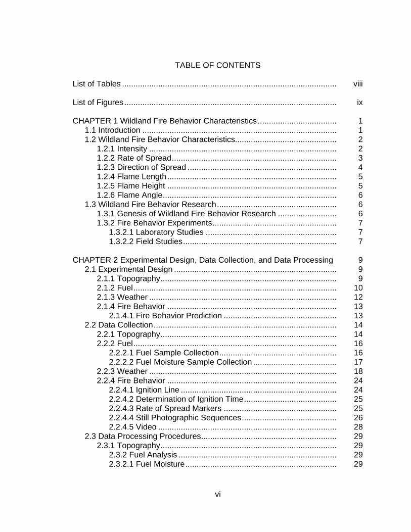
TABLE OF CONTENTS

List of Tables ............................................................................................... viii

List of Figures ..............................................................................................

ix

CHAPTER 1 Wildland Fire Behavior Characteristics ................................... 1 1.1 Introduction ...................................................................................... 1 1.2 Wildland Fire Behavior Characteristics............................................. 2

1.2.1 Intensity ................................................................................... 2 1.2.2 Rate of Spread ......................................................................... 3 1.2.3 Direction of Spread .................................................................. 4 1.2.4 Flame Length ........................................................................... 5 1.2.5 Flame Height ........................................................................... 5 1.2.6 Flame Angle ............................................................................. 6

1.3 Wildland Fire Behavior Research ..................................................... 6 1.3.1 Genesis of Wildland Fire Behavior Research .......................... 6 1.3.2 Fire Behavior Experiments ....................................................... 7

1.3.2.1 Laboratory Studies .......................................................... 7 1.3.2.2 Field Studies .................................................................... 7

CHAPTER 2 Experimental Design, Data Collection, and Data Processing 9

2.1 Experimental Design ........................................................................ 9 2.1.1 Topography .............................................................................. 9 2.1.2 Fuel .......................................................................................... 10 2.1.3 Weather ................................................................................... 12 2.1.4 Fire Behavior ........................................................................... 13

2.1.4.1 Fire Behavior Prediction .................................................. 13 2.2 Data Collection ................................................................................. 14

2.2.1 Topography .............................................................................. 14 2.2.2 Fuel .......................................................................................... 16

2.2.2.1 Fuel Sample Collection .................................................... 16 2.2.2.2 Fuel Moisture Sample Collection ..................................... 17

2.2.3 Weather ................................................................................... 18 2.2.4 Fire Behavior ........................................................................... 24

2.2.4.1 Ignition Line ..................................................................... 24 2.2.4.2 Determination of Ignition Time ......................................... 25 2.2.4.3 Rate of Spread Markers .................................................. 25 2.2.4.4 Still Photographic Sequences .......................................... 26 2.2.4.5 Video ............................................................................... 28

2.3 Data Processing Procedures ............................................................ 29 2.3.1 Topography .............................................................................. 29

2.3.2 Fuel Analysis ...................................................................... 29 2.3.2.1 Fuel Moisture ................................................................... 29

vii

2.3.2.2 Fuel Type......................................................................... 31 2.3.3 Weather ................................................................................... 36

2.3.3.1 Synoptic Conditions ......................................................... 36 2.3.3.2 Sounding ......................................................................... 38 2.3.3.3 Sodar .............................................................................. 40 2.3.3.4 Lidar ................................................................................ 40 2.3.3.5 AWS ................................................................................ 42 2.3.3.6 Micromet Sonics .............................................................. 43

2.3.4 Fire Behavior ........................................................................... 44 2.3.4.1 Fire Boundary Determination ........................................... 44 2.3.4.2 Flame Height and Flame Length Determination .............. 51 2.3.4.3 Heat Flux .........................................................................

52

CHAPTER 3 Observed Fire Behavior .......................................................... 53 3.1 Rate of Spread (ROS) ...................................................................... 53 3.2 Direction of Spread .......................................................................... 55 3.3 Flame Length, Flame Height, Flame Angle ...................................... 57 3.4 Fire Perimeter and Fire Area ............................................................

58

CHAPTER 4 Analysis of Fire Behavior ........................................................ 61 4.1 Fire Behavior Prediction (BehavePlus)............................................. 61 4.2 Observed vs. Predicted Fire Behavior ..............................................

63

CHAPTER 5 Summary, Conclusions, Limitations of Study, Further Research .....................................................................................................

65

5.1 Summary .......................................................................................... 65 5.2 Conclusions ...................................................................................... 66 5.3 Limitations of the Study .................................................................... 67 5.4 Further Research / Next Steps .........................................................

68

Acknowledgements ..................................................................................... 69 References ..................................................................................................

70

Appendices Appendix A – Video Segment Metadata ................................................ 75 Appendix B – Photograph / Georeferenced Photo / Fire Line Boundary 77 Appendix C - Georeference Points FHL Site 1 ....................................... 89

viii

LIST OF TABLES

Table 1 - Geographic Instrument Selection and Data Collected ......................... 15

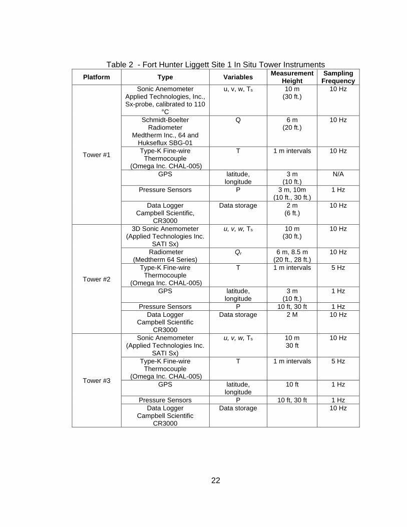
Table 2 - Fort Hunter Liggett Site 1 In Situ Tower Instruments .......................... 22

Table 3 - Fort Hunter Liggett Site 1 Non-Tower In Situ Instruments ................... 23

Table 4 – Fort Hunter Liggett Site 1 Remote Sensing Instruments..................... 23

Table 5 - Fort Hunter Liggett Site 1 Rate of Spread (ROS) Markers .................. 25

Table 6 - Cameras .............................................................................................. 26

Table 7 – Video Recorders ................................................................................. 28

Table 8 - Site 1 Fuel Moisture............................................................................. 31

Table 9 - Biomass Fuel Loading Fort Hunter Liggett Site 1 ................................ 32

Table 10 - Video Segment Metatdata Summary ................................................. 45

Table 11 - Video Segment 1 Image Times ......................................................... 46

Table 12 - ArcGIS Layer Definitions ................................................................... 47

Table 13 - Sample Georeference Points (Minute 4) ........................................... 49

Table 14 - Calculated Rate of Spread per minute ............................................... 54

Table 15 - Direction of Maximum Fire Spread (in degrees) ................................ 56

Table 16 – Observed Flame Height, Length, and Angle at Each Minute ............ 58

Table 17 – Observed Fire Perimeter and Area at Each Minute .......................... 59

Table 18 - BehavePlus Fire Prediction for Ignition to Tower 1 ............................ 61

Table 19 - BehavePlus Fire Prediction for Tower 1 to Tower 3 .......................... 62

Table 20 - Figures created by team members .................................................... 69

ix

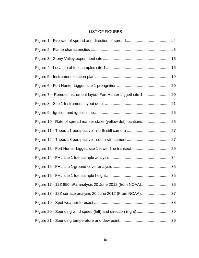
LIST OF FIGURES

Figure 1 - Fire rate of spread and direction of spread ........................................... 4

Figure 2 - Flame characteristics ........................................................................... 5

Figure 3 - Stony Valley experiment site .............................................................. 15

Figure 4 - Location of fuel samples site 1 ........................................................... 16

Figure 5 - Instrument location plan ..................................................................... 19

Figure 6 - Fort Hunter Liggett site 1 pre-ignition ................................................. 20

Figure 7 – Remote instrument layout Fort Hunter Liggett site 1 ......................... 20

Figure 8 - Site 1 Instrument layout detail ............................................................ 21

Figure 9 - Ignition and ignition line ...................................................................... 25

Figure 10 - Rate of spread marker stake (yellow dot) locations .......................... 26

Figure 11 - Tripod #1 perspective - north still camera ........................................ 27

Figure 12 - Tripod #3 perspective - south still camera ........................................ 27

Figure 13 - Fort Hunter Liggett site 1 tower line transect .................................... 29

Figure 14 - FHL site 1 fuel sample analysis ........................................................ 34

Figure 15 - FHL site 1 ground cover analysis ..................................................... 35

Figure 16 - FHL site 1 fuel sample height ........................................................... 35

Figure 17 - 12Z 850 hPa analysis 20 June 2012 (from NOAA)........................... 36

Figure 18 - 12Z surface analysis 20 June 2012 (From NOAA) ........................... 37

Figure 19 - Spot weather forecast ...................................................................... 38

Figure 20 - Sounding wind speed (left) and direction (right) ............................... 39

Figure 21 - Sounding temperature and dew point............................................... 39

x

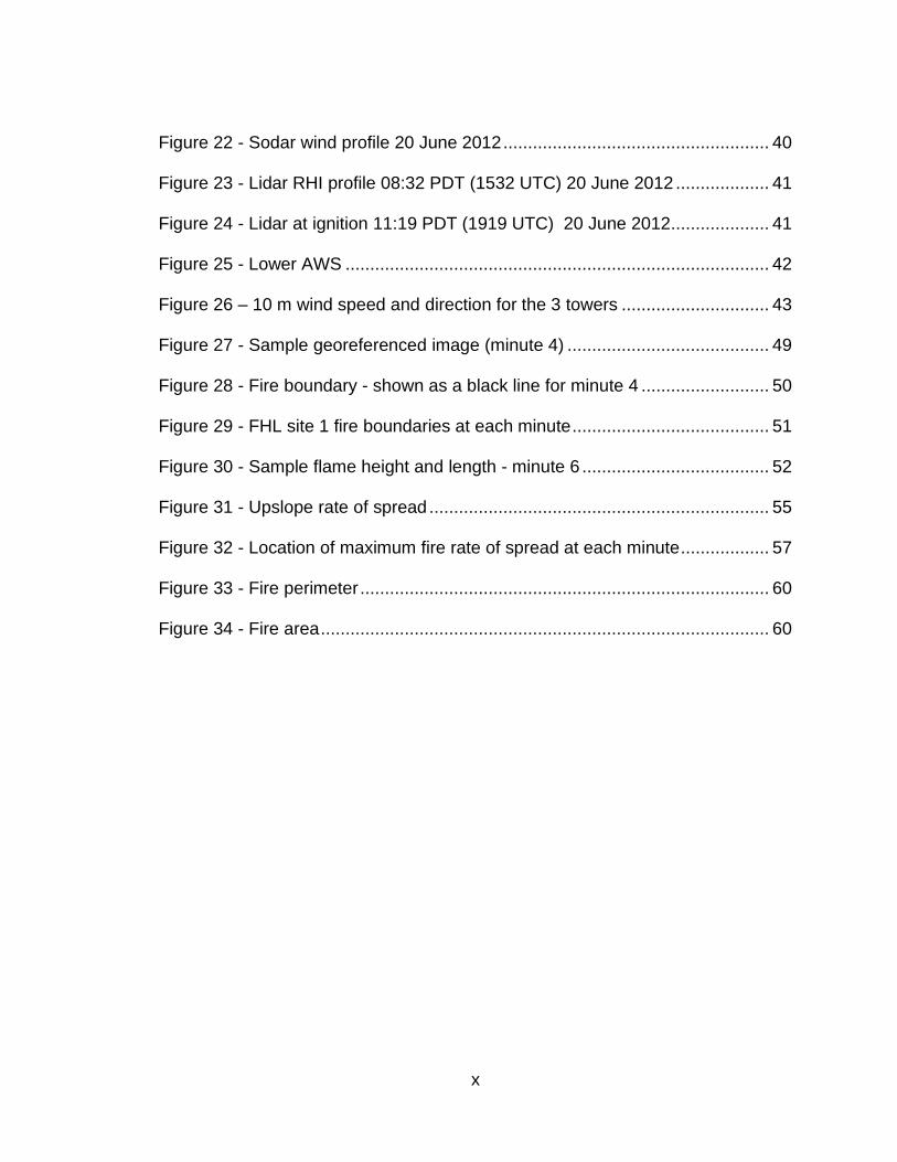
Figure 22 - Sodar wind profile 20 June 2012 ...................................................... 40

Figure 23 - Lidar RHI profile 08:32 PDT (1532 UTC) 20 June 2012 ................... 41

Figure 24 - Lidar at ignition 11:19 PDT (1919 UTC) 20 June 2012.................... 41

Figure 25 - Lower AWS ...................................................................................... 42

Figure 26 – 10 m wind speed and direction for the 3 towers .............................. 43

Figure 27 - Sample georeferenced image (minute 4) ......................................... 49

Figure 28 - Fire boundary - shown as a black line for minute 4 .......................... 50

Figure 29 - FHL site 1 fire boundaries at each minute ........................................ 51

Figure 30 - Sample flame height and length - minute 6 ...................................... 52

Figure 31 - Upslope rate of spread ..................................................................... 55

Figure 32 - Location of maximum fire rate of spread at each minute .................. 57

Figure 33 - Fire perimeter ................................................................................... 60

Figure 34 - Fire area ........................................................................................... 60

1

CHAPTER 1 Wildland Fire Behavior Characteristics

1.1 Introduction

Fire is a complex chemical reaction involving rapid oxidation of fuel to

generate heat and light. This relationship is often represented as a fire triangle

consisting of heat, fuel and oxygen, or as the fire tetrahedron consisting of these

three factors with the addition of the chemical chain reaction (IFSTA 2013).

Wildland fire is a subset of fire that occurs in undeveloped areas (NWCG 1996).

Wildland fire behavior results not only from complex reactions to create fire itself,

but is also influenced by the interactions between fuels, topography, and

weather. This relationship between fuels, topography and weather is referred to

as the wildland fire triangle (NWCG 1996).

Fire behavior on sloped terrain differs from that on flat ground as both the

intensity and the rate of spread (ROS) increase as the slope angle increases

(McArthur 1967; Rothermel 1972; Linn 2010). While there have been both

laboratory studies (Weise 1996, 1997) and field studies (Clements and Seto

2015) focused on fire behavior on slopes, there have been comparatively few

field studies that have measured the fire’s rate of spread simultaneously with

micrometeorology of the near surface environment at the fire front. The FireFlux

and FireFlux II experiments measured fire-atmosphere interactions of a head fire

passage in grass fuels with no slope (Clements 2006, Clements 2007, Clements

2008, Clements et al. 2019). Additionally, most field studies have been

conducted utilizing backing fires, i.e., fires that spread downslope or into the

2

wind, rather than heading fires, i.e., fires that spread into the wind or upslope;

thus, the data obtained do not represent the actual atmospheric environment of

wildfires.

1.2 Wildland Fire Behavior Characteristics

Wildland fire behavior is generally described in terms of intensity, rate of

spread, and direction of spread (Rothermel 1972). Other useful measures of

wildland fire behavior are flame length, flame height, and flame angle.

1.2.1 Intensity

There has been a great deal of discussion on how to define and measure fire

intensity, and this has resulted in some confusion about the meaning of the term.

Fire intensity can be broadly thought of as the energy released during a fire.

However, fire intensity, fireline intensity, reaction intensity, temperature,

residence time and radiative energy are just a few of the metrics that have been

to describe the energy released from a fire (Keeley 2009).

In physics, ‘intensity’ is defined as the time-averaged energy flux (Bird et al.

1960). Since flux is a measure of the flow rate per unit area, intensity becomes

the time-averaged energy flow rate per unit area. This means that intensity

describes the amount of energy transferred as the fire moves. This energy is

transferred into the environment (released) as organic matter pyrolyzes and the

resulting vapors combust. In an environment absent of wind, the energy transfer

is through radiation and is measured as radiative flux. When wind occurs in the

same direction as fire spread, convective energy transfer becomes a factor to

3

consider and convective flux must be added to the fire behavior model (Frandsen

1971; Rothermel 1972). When the energy measured is restricted to the infrared

spectrum, the energy transport can be described as radiative heat flux.

The closest alignment in fire behavior with the meaning of intensity as

described in physics is Rothermel’s term, ‘reaction intensity’ (Rothermel 1972)

Reaction intensity is defined as the heat release rate per unit area (W m-2) at the

fire front, and is the heat source for Rothermel’s fire spread model.

Byram (1959) defines intensity as ‘fireline intensity’. Fireline intensity is the

rate of heat transfer per unit length of the fire line (kW m-1). Both conductive and

radiative heat transfer are included in Byram’s fireline intensity measure.

However, there are several fire effects that cannot be fully predicted using

either Rothermel’s or Byram’s definitions of intensities. For example, neither of

these measures alone is a predictor of how much total heat the vegetation will be

exposed to during the fire front passage. The total heat exposure is necessary to

understand the amount of vegetation that will be consumed or damaged as the

fire front passes. Another concern with both of these definitions is that the

resulting values are difficult to translate into visual indicators and thus do not

serve as useful tools for assessing fire behavior by on-the-ground fire fighters at

active fires.

1.2.2 Rate of Spread

Show (1919) proposed three different ways to measure the rate of spread of a

fire: linear distance from the point of origin, area burned, and fire perimeter

4

(Figure 1). Linear distance from the point of origin helps determine the rate of

spread at the fire front and thus determines the type of firefighting resources

(manpower, engines or aircraft) required. Fire perimeter is generally used to

determine the number of firefighting resources required to manage the fire since

the resources required are proportional to the perimeter (Potter 2012a). Area

burned is useful for determining the total number of acres affected and thus the

resources required to rehabilitate the fire area.

Figure 1 - Fire rate of spread and direction of spread

1.2.3 Direction of Spread

The direction of spread is measured on four flanks: head, left, right, and heel

(Figure 1). The head of the fire is the main direction of spread and is generally

the direction of most rapid fire spread. The head fire direction of spread is

generally in the direction of the wind and upslope. The left flank and right flank

are progressions that are perpendicular to the main fire spread. The heel of the

fire proceeds in the opposite direction of the head fire, is slower, and generally

5

exhibits backing fire behavior in that the fire progresses into the wind or

downslope.

1.2.4 Flame Length

Flame length (Figure 2) is the distance of the flame from the base of the flame

to the tip of the flame. If the flame is not influenced by wind, the flame will be

vertical, and the flame length will be the vertical length of the flame. However, if

the flame is influenced by wind, the flame is deflected from the vertical and the

flame length will increase and become larger than the vertical distance. Flame

length helps determine the heat transfer and thus the rate of spread of a fire

(Weise 1996).

Figure 2 - Flame characteristics

1.2.5 Flame Height

Flame height (Figure 2) is the vertical distance from the base of the flame to

the tip of the flame. Flame height and flame length will be the same if the fire is

not influenced by wind; however, under the influence of wind, the flame will be

deflected from the vertical and the flame length will increase while the flame

height may stay the same.

6

1.2.6 Flame Angle

When a flame is influenced by wind, the flame will be deflected from the

vertical. Flame angle (Figure 2) is measured from a vertical line to the middle of

the flame (Weise 1996). Flame angle is linked with flame length when

determining the radiative heat transfer of fires to unburned fuels.

1.3 Wildland Fire Behavior Research

1.3.1 Genesis of Wildland Fire Behavior Research

The United States Forest Service (USFS) established the Priest River Forest

Experiment Station to study forest fire behavior after the Big Burn of 1910 burned

3 million acres of forest in Northern Idaho, Western Montana, and Eastern

Washington in the United States and Southeast British Columbia in Canada. 87

people were killed in this fire, including 78 fire fighters. The goal of the research

was to predict the conditions for increased fire danger and thus serve as a

warning system for the USFS. The National Fire Danger Rating System

(NFDRS) was one of the results of this research (Hardy 1977). The NFDRS uses

weather observations, fuel type, and fuel condition to predict the potential fire

intensity in specific geographic areas in the USA (Schlobohm 2002).

The importance of understanding wildland fire behavior was reemphasized in

1949 after 13 firefighters died while trying to outrun a fire front that was

accelerating up a slope in the Mann Gulch Fire in Montana, USA. The

supervisor, Wagner Dodge, lit a fire around him. He survived as the main fire

went around the burned-out area he had created. Two other firefighters survived

7

because they were able to get to a rockslide on the other side of the ridge. All

three survived because they were able to break the wildland fire triangle by

removing the fuel (MacLean 1992). After this tragedy, the US Forest Service set

up three additional research labs: Macon, Georgia in 1959; Missoula, Montana in

1960; and Riverside, California in 1962, to study fire behavior.

1.3.2 Fire Behavior Experiments

1.3.2.1 Laboratory Studies

Much fire behavior experimentation has been done in laboratories (Fons

1946; Anderson et al. 1966; Rothermel and Anderson 1966; Thomas 1971; Albini

1976; Nelson and Adkins 1988; Wolff 1991; Beer 1993; Weise 1996; Wu et al.

2000; Mendes-Lopes et al. 2003; Anderson et al. 2006; Dupuy et al. 2011). This

research has contributed to understanding the behavior of fire in a laboratory

environment but does not take into account fire-atmospheric interactions.

1.3.2.2 Field Studies

Collecting data sets for actual wildland fire is difficult due to the environmental

and logistical constraints. Wildland fires generally occur in very complex terrain

which increases the variability of the input conditions and further complicates the

fire behavior analysis. It is difficult to collect the initial conditions at the time and

location of the ignition since fires may go undetected for a period of time, so the

initial conditions are often not known.

Show (1919) performed initial field experiments to document the effect of

wind on fire spread. However, although the experiment sites had different

8

slopes, he averaged the slopes of all the sites and used this average for his

calculations, thus removing slope as a variable. Gray (1933) determined that fuel

composition, fuel moisture, air movement, and topographic slope were

independent variables affecting the rate of spread of a fire. Curry and Fons

(1938, 1940) determined a curvilinear relationship between wind and slope. At

low wind speeds, slope is a minor factor, but as the wind speed increases, slope

increasingly becomes important. If the wind is in the direction of upslope, then

the influence is maximized. McArthur (1967, 1969) studied several grassfires in

Australia and observed relationships between weather and fire behavior.

Thomas (1967, 1971) studied both laboratory and controlled burns in Australia

and developed rate of spread predictions.

Several field experiments have been conducted more recently including:

FireFlux, Houston, TX, 2006; FireFlux II, Houston TX, 2013; RxCADRE, Elgin

Airforce Base, FL, 2008, 2011, 2012; Camp Parks, Dublin, CA, 2010, resulting in

an increased understanding of fire-atmospheric interaction on fire behavior

(Clements, 2007, 2014; Ottmar, et al., 2016; Clements and Seto, 2015). Of

these experiments, all but the Camp Parks experiment were conducted on flat

terrain, so slope had not been a factor until the Camp Parks experiment. The

Camp Parks experiment was on a slope and was a test case to determine how to

instrument a fire with in situ instruments. Many of the lessons learned in that

experiment were used to improve the experimental design of the Fort Hunter

Liggett (FHL) slope fire experiment, which is the topic of the current work.

9

CHAPTER 2 Experimental Design, Data Collection, and Data Processing

2.1 Experimental Design

The goal of this experiment was to observe fire behavior for a head fire on a

slope, and to generate data sets for that fire. These data sets include

measurements of the three factors that dictate wildland fire behavior: topography,

fuels, and weather. Additionally, the data sets include the measurements of the

resulting fire behavior: rate of spread, flame height, flame length, flame angle,

and fireline intensity. Since fire-atmospheric interactions were the focus of this

experiment, the other variables influencing fire behavior were to be kept as

constant as possible throughout the experiment.

2.1.1 Topography

The topography is the lay of the land and is the least variable factor in

wildland fire behavior (NWCG 1996). Topography of an area is not generally

thought of as variable because large influences such as earthquakes, slides, or

mechanical grading are required to change it. Topographic features of interest

are the slope angle and the aspect.

When fire changes from burning on flat land and starts burning up a slope,

the rate of spread increases. When the slope reaches 10°, the rate of spread is

approximately double that on flat land. The rate of spread doubles again on 20°

slopes (McArthur 1967). When the slope angle reaches 24°, more of the flame is

in direct contact with the slope and the flame is considered attached to the slope.

This increases the rate of heating of the fuels and fire behavior becomes

10

explosive with dramatic increases in rate of spread upslope (Wu et al. 2000, Dold

et al. 2009).

The aspect refers to the Cartesian direction the slope faces. In the northern

hemisphere, south aspect slopes receive the most direct sunlight as compared

with other aspects (NWCG 1996). This increased insolation causes southern

and western aspect slopes to be drier, resulting in generally lighter fuel loads.

The drier, lighter fuel load is more available to burn and can contribute to rapidly

spreading fires (NWCG 1996).

A uniform slope was required to control for the variability of a change in slope

on fire behavior. A hill with a 20° slope was desired for the experiment to give a

high rate of spread, but keep the fire behavior below the explosive level. A south

or west aspect was desired to ensure a light and uniform fuel load.

2.1.2 Fuel

The fuel is the vegetation that will burn. Wildland vegetation types vary from

light grasses to shrubs to forests (NWCG 1996). The intensity of the fire varies

with both the amount of fuel, or fuel loading, and with the characteristics of the

fuel (Rothermel and Anderson 1966). There are numerous characteristics, but

those that seem to influence fire behavior the most are fuel moisture content,

chemical properties such as oil content, and available surface area (Anderson

1982). The fuel is subject to seasonal variation as more fuels tend to be dryer

and ready to burn, referred to as fuel availability, in the summer and fall than

during winter and spring (Scott and Burgan 2005). The various types of fuels

11

have been studied and similar characteristics were found. Fuels with similar

characteristics were grouped together and classified as a fuel model since they

would exhibit similar fire behavior. Thirteen (13) fuel models were originally

developed (Anderson 1982) and then these models were further refined and

expanded upon into the 42 Standard Fire Behavior Fuel Models (Scott and

Burgan 2005).

Fuel is moderately variable as generally the same fuel will be found from year

to year in the same geographic area, but the fuel moisture content will vary as

the drying season progresses and thus change the availability of the fuel.

A uniform fuel bed was desired to control for fuel variability. Grass is a very

common fuel and it is easy to see its underlying topography. Grass fires are

easy to ignite, burn quickly, and are relatively easy to control once lit, so a grass

fuel bed was desired. Samples of grass from the experiment site need to be

collected and analyzed to determine the fuel characteristics. Fuel properties of

interest are: fuel bed depth, the average height of the fuel above the ground; fuel

loading, the amount of fuel present expressed as weight per unit area; and

percentage fuel moisture content, the amount of moisture present in a fuel

expressed as a percentage fuel after it has been dried in an oven. Another

reason to select a grass fuel is that it represents a light flashy fuel which is a

common denominator of fatality fires (Wilson 1977). An understanding of the fire

behavior in these fuel types may lead to increased fire fighter safety (Butler,

2014).

12

2.1.3 Weather

Weather is the state of the atmosphere and is described in terms of the short-

term (minutes to days) variations in the atmosphere such as temperature,

humidity, precipitation, cloudiness, visibility, and wind (American Meteorological

Society 2019).

The weather factors that most strongly influence fire behavior are wind speed,

wind direction, temperature, humidity, and insolation (NWCG 1996). Wind speed

influences the rate of spread of the fire. Wind direction influences the direction of

fire spread. Air temperature, humidity, and insolation affect the fuel moisture and

thus the availability of the fuel to burn (Potter 2012a). Weather is the most

variable of the three wildland fire factors.

The ideal conditions for the experiment would be to have no wind. Then the

wind could be removed as a factor in the fire behavior calculations, and the

direction of spread of the fire would be due only to other factors, in particular -

slope. The next most desirable condition would be to have the wind aligned with

the upslope direction. The theory is that the slope becomes a multiplier for the

effect of the wind. When the wind is at an angle to the slope, then the direction

of fire spread is affected by both the wind and the slope (McArthur 1967;

Rothermel 1972).

Since the mechanisms of fire-atmospheric interactions are only partially

understood (Werth et al. 2011, Potter, 2012a), a wide range of instruments from

the synoptic scale to the micrometeorological scale were selected to obtain as

13

much meteorological data as possible. Both in situ instruments and remote

sensing instruments were deployed due to the possibility of the in situ

instruments being damaged during the fire front passage, as experienced in the

Camp Parks experiment (Clements and Seto 2015).

The in situ instruments included: 3-D sonic anemometers; radiometers;

thermocouple arrays; pressure sensors, and a radiosonde balloon sounding

system. The remote sensing instruments included: a Doppler Wind Lidar; a

microwave temperature profiler; and an acoustic wind profiler.

2.1.4 Fire Behavior

The rate of spread (ROS) and direction of spread of the fire front can be

obtained from video recordings and still camera photographs of the fire. The

flame characteristics of flame height, flame length, and flame angle can be

estimated from the still camera photographs. Both radiative and convective heat

transfer, generally combined and expressed as fire line intensity (heat per unit

length of the fire line per second) (Byram 1959), can be calculated from the

radiative flux and heat flux measurements from the radiometers and sonic

anemometers.

2.1.4.1 Fire Behavior Prediction

Papadopoulos and Pavlidou (2011) described several software programs

currently available to predict wildland fire behavior. The program BehavePlus

(Andrews et al., 2005) was selected to provide a prediction of the fire behavior to

aid in the instrument placement during the experimental design. The actual

14

results could also then be compared with the prediction. BehavePlus was

selected because it is a simple fire behavior prediction program that runs on a

desktop or laptop computer and is commonly used in the field during campaign

fires. An app version that runs on the iPhone (Covele 2008) is also available.

Given a set of easily measured inputs for topography, fuel and weather,

BehavePlus predicts several properties of fire behavior such as the rate of

spread, the direction of spread, the flame height, and the fire intensity. The slope

angle (in degrees) and slope aspect are obtained from the topographical maps.

The fuel model number and fuel moisture percentage are provided by the fuel

sample analysis, and the horizontal wind speed and direction come from the

meteorological instruments surrounding and within the experiment plot.

2.2 Data Collection

The instruments required to collect data to measure the topographic features,

fuel characteristics, atmospheric condition, and fire behavior are detailed in this

section.

2.2.1 Topography

The experimental site selected was a small ridge in the Stony Valley of Fort

Hunter Liggett, Monterey County, California (Figure 3). The ridge was grass

covered, had a west aspect, and had slope angles between 10o and 20o.

The overall topographical data was obtained from the USDA (United States

Department of Agriculture) Alder Peak Quadrangle Topographic Map and from

GIS (Geographic Information Systems) data supplied by Fort Hunter Liggett. The

15

detailed instrument locations, topographic feature locations, and fire ignition line

location were obtained using GPS (Global Positioning System) instruments

detailed in Table 1.

Table 1 - Geographic Instrument Selection and Data Collected

Data Type Instrument Data Collected

Geographic Data

Trimble GPS Boundaries of patches of different fuel type, fuel sample locations,

instrument locations, marker locations

Geographic Data

Garmin GPS Model 60CSx

Fire ignition line

Figure 3 - Stony Valley experiment site

16

2.2.2 Fuel

2.2.2.1 Fuel Sample Collection

Twenty (20) plots were selected from within the experiment site for sampling

to determine the fuel characteristics. These plots were to the south of the line

defined by 3 in situ towers which held the meteorological instruments and were in

a line from the base of the hill to the top of the hill. The fuel sampling locations

for plots 1-18 are shown in Figure 4. GPS locations of Plot 19 and Plot 20 were

not obtained, but they were located 30 ft (10 m) east of the original fuel sampling

line coming back down the hill. Each plot was spaced 30 ft (10 m) from the

previous plot further up the hill, measured from the lower edge of the sample

square to the lower edge of the next sample square. A GPS location of each plot

was recorded using the lower left corner of the plot frame as facing up the hill, or

the NW corner of the plot.

Figure 4 - Location of fuel samples site 1

Due to the amount of fuel and the observed uniformity of the fuel, only a half

meter square sample size was required for each fuel sample plot. A 0.5 x 0.5 m

17

PVC frame was placed on the ground at each plot location, resulting in a

sampling area of 0.25 m2. The vegetation bounded by the PVC fame was then

collected. Only the vegetation that was in the vertical column created by the

frame was collected. For example, if the grass roots were outside the frame and

the grass stem was partially inside the frame and partially outside the frame, the

portion of grass stem that was within the frame was collected and the portion of

grass stem outside the frame was not collected. Since this site contained only

grass, it was not necessary to separate the vegetation types into grass, forbs

(herbaceous flowering plant), shrubs, etc. Only the vegetation from above the

soil layer was collected, i.e., no soil or roots of the grass were collected. Each

sample was placed in a brown paper bag and labeled with the collection site and

plot number.

The fuel sample collection and subsequent fuel loading calculations for the

fuel samples were performed by a team from the US Forest Service Pacific

Northwest Research Station, Pacific Wildland Fire Sciences Laboratory. The

collection was performed on 30 May 2012.

2.2.2.2 Fuel Moisture Sample Collection

Ten (10) fuel samples were collected on the morning of the experiment, June

20, 2012, at 09:45 PDT (16:45 UTC). Each fuel sample was collected from one

of the first ten orange marker stakes on the tower line on the slope (Figure 4).

The exact locations were not significant, as the intent was to obtain an

approximate average fuel moisture content for the fuel bed. The locations of

18

these markers are shown in Figure 7. Each sample consisted of a one gallon,

plastic, sealable bag filled with grass clippings from the experiment site. Each

bag was tightly sealed at the site and then stored in a cool place until it could be

processed. The amount of fuel in each bag varied from 21 g to 35 g. The

amount was not material as long as each bag was reasonably full since fuel

moisture calculations depend only on the difference in weight between the

undried sample and the dried sample.

2.2.3 Weather

The experiment measured weather conditions from synoptic scale to

micrometeorological scale. For the synoptic scale, a balloon radiosonde system

was launched on the morning of the experiment, a fire spot weather forecast was

requested from the National Weather Service (NWS) in Monterey, CA, and the

NWS upper level maps were obtained for the day of the experiment.

For the local weather conditions, two standard Automated Weather Stations

(AWS) were deployed, one at the bottom of the slope and one at the top of the

slope. The CSU-MAPS (California State University Mobile Atmospheric Profiling

System) designed by Clements and Oliphant (2014) was also deployed. This

system includes a scanning doppler wind Lidar (LIght Detection And Ranging), a

microwave profiling radiometer, both deployed west of the experiment site, and a

32 m micromet tower deployed south of the experiment site. A doppler mini

sodar (SOnic Detection And Ranging) was also deployed south of the experiment

site. The data collected by micromet tower was not used in this analysis. Sonic

19

anemometers mounted on each of the three towers within the experiment site

measured the micrometeorological conditions of temperature and u, v, and w

winds within the fire.

The planned instrument locations are shown in Figure 5, the location of the

remote sensing instrument in Figure 7, and instruments within the plot in Figure

8. A brief description of the specific instruments deployed and the data each was

intended to collect are detailed in Table 2, Table 3, and Table 4. A photo of the

completely instrumented site before ignition is shown in Figure 6.

Figure 5 - Instrument location plan

20

Figure 6 - Fort Hunter Liggett site 1 pre-ignition

Figure 7 – Remote instrument layout Fort Hunter Liggett site 1

21

Figure 8 - Site 1 instrument layout detail

22

Table 2 - Fort Hunter Liggett Site 1 In Situ Tower Instruments

Platform Type Variables Measurement

Height Sampling

Frequency

Tower #1

Sonic Anemometer Applied Technologies, Inc., Sx-probe, calibrated to 110

°C

u, v, w, Ts 10 m (30 ft.)

10 Hz

Schmidt-Boelter Radiometer

Medtherm Inc., 64 and Hukseflux SBG-01

Q 6 m (20 ft.)

10 Hz

Type-K Fine-wire Thermocouple

(Omega Inc. CHAL-005)

T 1 m intervals 10 Hz

GPS latitude, longitude

3 m (10 ft.)

N/A

Pressure Sensors P 3 m, 10m (10 ft., 30 ft.)

1 Hz

Data Logger Campbell Scientific,

CR3000

Data storage 2 m (6 ft.)

10 Hz

Tower #2

3D Sonic Anemometer (Applied Technologies Inc.

SATI Sx)

u, v, w, Ts 10 m (30 ft.)

10 Hz

Radiometer (Medtherm 64 Series)

Qr 6 m, 8.5 m (20 ft., 28 ft.)

10 Hz

Type-K Fine-wire Thermocouple

(Omega Inc. CHAL-005)

T 1 m intervals 5 Hz

GPS latitude, longitude

3 m (10 ft.)

1 Hz

Pressure Sensors P 10 ft, 30 ft 1 Hz

Data Logger Campbell Scientific

CR3000

Data storage 2 M 10 Hz

Tower #3

Sonic Anemometer (Applied Technologies Inc.

SATI Sx)

u, v, w, Ts 10 m 30 ft

10 Hz

Type-K Fine-wire Thermocouple

(Omega Inc. CHAL-005)

T 1 m intervals 5 Hz

GPS latitude, longitude

10 ft 1 Hz

Pressure Sensors P 10 ft, 30 ft 1 Hz

Data Logger Campbell Scientific

CR3000

Data storage 10 Hz

23

Table 3 - Fort Hunter Liggett Site 1 Non-Tower In Situ Instruments

Platform Type Variables Measurement

Height Sampling

Frequency

AWS 1 (ignition line)

CS215 Campbell Scientific

T, RH 2 m 5 minutes

Wind Sentry Model 03002 R.M Young

WS, WD 2 m 5 minutes

CS1000 Datalogger Data storage 2m N/A

AWS 2 (top of slope)

CS215 Campbell Scientific

T, RH 2m 5 minutes

Wind Sentry Model 03002 R.M Young

WS, WD 2m 5 minutes

CS1000 Datalogger Data storage 2 m N/A

FireBoxes

SJSU custom design

P 10 ft. (3 m) 2 Hz

T 10 ft. (3 m) 2 Hz

RH 10 ft. (3 m) 2 Hz

GPS latitude, longitude

10 ft. (3 m) 1 Hz

Radiosonde System

Vaisala Inc RS-92GPS WS, WD, P, RH, T, GPS location

1 Hz

Table 4 – Fort Hunter Liggett Site 1 Remote Sensing Instruments

Platform Type Variables Measurement

Height (m AGL)

Sampling Frequency

CSU- MAPS 32-m

extendable tower

Thermistor–hygristor sensors

(Vaisala, Inc. HMP45C)

T, RH 1 m intervals from 7 m to 31

m

1 min

3D sonic anemometers (RM Young 81000)

u, v, w, Ts 7 m and 31 m 10Hz

2D anemometers (Gill, WindSonic)

u, v 7m and 31 m 1Hz

Doppler LIDAR

Stream Line 75 Halo Photonics Ltd.

vr, β range gate: 18 1 Hz

Doppler Mini SoDAR

VT-1 (Atmospheric Research

and Technology)

u, v, w 15 – 200 m AGL

1 Hz

Microwave Profiler

MP-3000A (Radiometrics Inc)

T, RH 50 – 1x104 180s

Key: vr, radial velocity; β, aerosol backscatter intensity; CSU-MAPS, California State University – Mobile Atmospheric Profiling System; u horizontal streamwise velocity; v, horizontal cross-stream velocity; w, vertical velocity; Ts, sonic temperature; T, air temperature; Q, total heat flux, Qr, radiative heat flux, RH, relative humidity; WS, wind speed; WD, wind direction; P, atmospheric pressure

24

2.2.4 Fire Behavior

2.2.4.1 Ignition Line.

A firing crew from Fort Hunter Liggett Fire Department used a drip torch with

the standard 3:1 diesel:gas fuel ratio to ignite the fire. The firefighter setting the

fire had a hand-held GPS on his web gear set to capture his position 10 times

every second so that the exact ignition line was measured. The line initiated to

the north of the tower line marker and moved southward along the road. The

experimental design assumed winds from the west or upslope. However, on the

day of the experiment, the wind was southwesterly, so the ignition line had to be

extended well past the initially planned line so that the fire would burn through

the meteorological towers if the direction of spread became wind dominated

rather than slope dominated.

There was a patch of mustard grass close to the road south of the

experimental plot. This mustard grass was a different fuel type than the grass in

the rest of the experimental plot, so the decision was made to take the ignition

line at an angle away from the road towards the hill crest and around the mustard

grass to eliminate any variability in the fuels. The firing was stopped just past the

mustard grass patch. The ignition line is shown as the solid black line in Figure

9.

25

Figure 9 - Ignition and ignition line

2.2.4.2 Determination of Ignition Time

To determine the exact ignition time, the camera used to photograph the

ignition was calibrated to the GPS clock on the lower AWS station. The fire was

ignited at 11:18:10 PDT (181810 UTC) on 20 June 2012.

2.2.4.3 Rate of Spread Markers

The 15 rate of spread marker stakes, shown as yellow dots in Figure 10, were

placed along the tower transect at 10 m intervals The measurement criteria are

shown in Table 5.

Table 5 - Fort Hunter Liggett Site 1 Rate of Spread (ROS) Markers

Platform Type Variables Measurement

Height Sampling Frequency

ROS Markers

1-15

marker stakes ROS (m s-1) 2 m 10 m increments

26

Figure 10 - Rate of spread marker stake (yellow dot) locations

2.2.4.4 Still Photographic Sequences

Three (3) still cameras were used to capture photographs of the fire during

the experiment. Table 6 gives the details on the cameras used.

Table 6 - Cameras

Platform Type Variables Measurement

Height Sampling Frequency

Tripod #1 (North Still)

Canon EOS 40D still-image, time-lapse, digital SLR

camera

Flame length m, flame height m,

flame angle

1.5 m 1Hz

Tripod #3 (South Still)

Canon EOS DIGITAL REBEL

XT still-image, time-lapse, digital SLR

camera

Flame length m, flame height m,

flame angle

1.5 m 1 Hz

Camera 1 (operated by

photographer)

Canon EOS 5D Mark II

still-image, time-lapse, digital SLR

camera

Various Varies Random

27

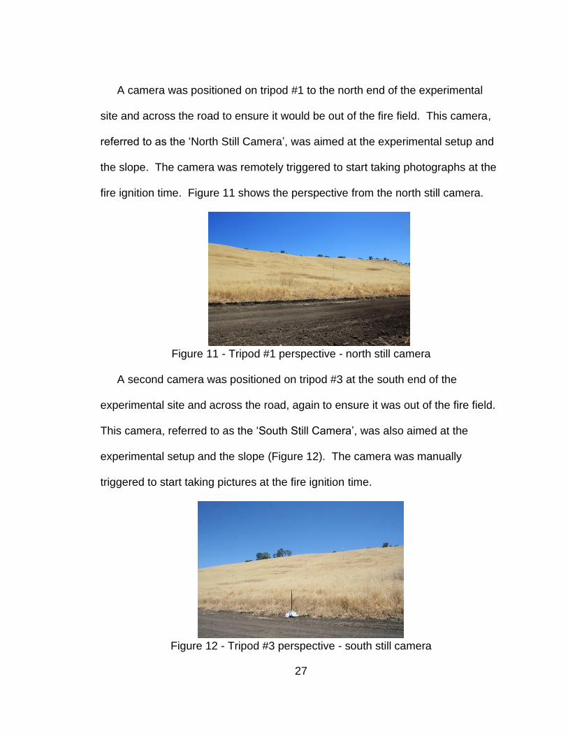
A camera was positioned on tripod #1 to the north end of the experimental

site and across the road to ensure it would be out of the fire field. This camera,

referred to as the ‘North Still Camera’, was aimed at the experimental setup and

the slope. The camera was remotely triggered to start taking photographs at the

fire ignition time. Figure 11 shows the perspective from the north still camera.

Figure 11 - Tripod #1 perspective - north still camera

A second camera was positioned on tripod #3 at the south end of the

experimental site and across the road, again to ensure it was out of the fire field.

This camera, referred to as the ‘South Still Camera’, was also aimed at the

experimental setup and the slope (Figure 12). The camera was manually

triggered to start taking pictures at the fire ignition time.

Figure 12 - Tripod #3 perspective - south still camera

28

A third camera, referred to as the “Mobile Camera”, was operated by a

photographer who walked along the road at the west end of the experimental

site. This photographer took photos of the fire behavior at differing zoom levels

and differing perspectives.

2.2.4.5 Video

Three (3) video recorders were deployed to capture video of the fire

experiment. Table 7 gives the details of those video recorders.

Table 7 – Video Recorders

Platform Type Variables Measurement

Height Sampling

Frequency

Airborne in helicopter

Cannon Digital Video Recorder

ROS m s-1 fire perimeter m,

fire area m2

300 m 30 Frames per second

Infrared Video Recorder (Flir)

ROS m s-1 fire perimeter m,

fire area m2

300 m 1 Frame per second

Tripod #2 Digital Video Recorder

ROS m s-1

flame height m, flame length m

1.5 m 30 and 60 Hz

A helicopter circled the fire from just before the ignition until the fire reached

the third micrometeorological tower. There were two photographers and

videographers onboard using the digital video recorder and the infrared video

recorder to record the fire experiment. The Infrared (IR) video camera failed to

record data, thus the IR data are not available.

A digital video camera was set up to the north of the instrumented slope on

the road to the west of the slope on tripod #2. This video recording was started

just before the fire ignition and videotaped the fire progression until the fire

reached the top of the slope after burning through the instrumented towers.

29

2.3 Data Processing Procedures

2.3.1 Topography

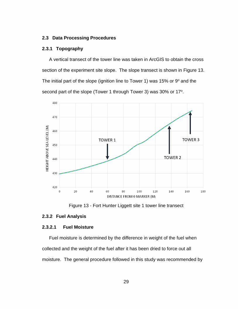
A vertical transect of the tower line was taken in ArcGIS to obtain the cross

section of the experiment site slope. The slope transect is shown in Figure 13.

The initial part of the slope (ignition line to Tower 1) was 15% or 9o and the

second part of the slope (Tower 1 through Tower 3) was 30% or 17o.

Figure 13 - Fort Hunter Liggett site 1 tower line transect

2.3.2 Fuel Analysis

2.3.2.1 Fuel Moisture

Fuel moisture is determined by the difference in weight of the fuel when

collected and the weight of the fuel after it has been dried to force out all

moisture. The general procedure followed in this study was recommended by

30

the US Forest Service Pacific Northwest Research Station, Pacific Wildland Fire

Sciences Laboratory (http://www.fs.fed.us/pnw/fera/).

Each of the 10 samples of fuel collected for fuel moisture analysis from site 1

was weighed and the weight recorded. Samples 1 through 7 were opened and

the open bags were placed in the Fire Lab Oven for the first batch. Some

samples from another experiment were also placed in the oven with these

samples. The process was to dry the samples at 70 °C for 48 hours.

Unfortunately, the lab oven malfunctioned, and the samples were subjected to

92 °C within 90 minutes of the start of the drying cycle. This excessive

temperature caused the plastic bags in which the samples were contained to

melt. The various samples were mixed and it was not possible to determine the

oven dry weight of the samples 1 through 7. Samples 8 through 10 were more

successfully dried after the Fire Lab oven was repaired. Table 8 shows the

results for the samples.

As a result, the fuel moisture value used for the fire behavior models was

1.6%. Simulations were also run using 2.25%, the average of samples 9 and 10.

31

Table 8 - Site 1 Fuel Moisture

Bag Pre Oven Weight

(g)

Post Oven

Weight (g)

Net Water Weight

(g)

Fuel Moisture (Water weight /

dry weight)

Note

1 30.1 *

Destroyed

2 32.5 *

Destroyed

3 30.5 *

Destroyed

4 28.1 *

Destroyed

5 26.1 *

Destroyed

6 21 *

Destroyed

7 21 *

Destroyed

8 33.7 32.5 1.2 3.7% Hole in bag absorbed moisture

from environment

9 24.7 24.3 0.4 1.6%

10 35.2 34.2 1 2.9% Grass in seal might be OK

2.3.2.2 Fuel Type

Each sample was weighed to determine the amount of biomass present. The

data are shown in Table 9. Standard fire behavior fuel models currently

employed in the United States express fuel loading as (US) tons / acre, so the

data are given in both SI (Système Internationale) and the standard

representation.

32

Table 9 - Biomass Fuel Loading Fort Hunter Liggett Site 1

Plot # g / 0.25 m2

US ton/acre

% Grass Cover % Bare Soil

Height (m)

Plot 1 193.14 3.45 100 0 0.8500

Plot 2 167.17 2.98 78 22 0.8600

Plot 3 160.87 2.87 100 0 0.7500

Plot 4 227.40 4.06 100 0 0.8600

Plot 5 154.17 2.75 95 0 0.8500

Plot 6 141.67 2.53 80 20 0.7112

Plot 7 138.75 2.48 95 5 0.7874

Plot 8 66.83 1.19 60 40 0.5842

Plot 9 118.11 2.11 95 5 0.7874

Plot 10 78.98 1.41 85 15 0.7112

Plot 11 122.58 2.19 90 10 0.8636

Plot 12 88.93 1.59 60 40 0.7874

Plot 13 50.13 0.89 30 40 0.5842

Plot 14 68.50 1.22 55 45 0.6604

Plot 15 53.36 0.95 40 60 0.5842

Plot 16 87.49 1.56 75 25 0.6858

Plot 17 83.31 1.49 60 40 0.8128

Plot 18 42.92 0.77 55 45 0.4064

Plot 19 56.26 1.00 30 70 0.6096

Plot 20 44.94 0.80 35 65 0.5588

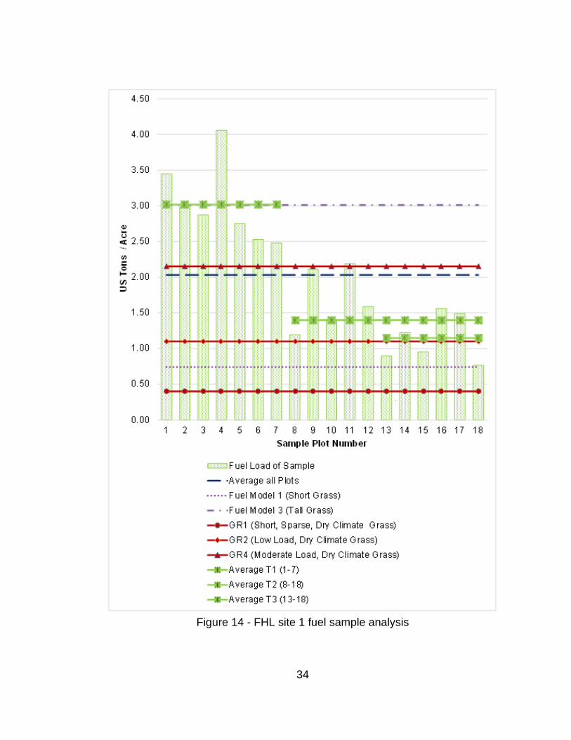
The tons per acre for the fuel samples are plotted in Figure 14. Samples from

Plot 19 and 20 were omitted from the analysis because when they were included,

the results were too heavily weighted towards the lower fuel loading at the top of

the hill. To determine if the fuel collected from FHL Site 1 could be represented

by an existing fuel model during the analysis phase, several fuel loadings from

existing models were chosen and also plotted on Figure 14 for reference. From

the grass group of Anderson (1982), Fuel Model 1 (FM1) Short Grass and Fuel

Model 3 (FM3) Tall Grass were selected. Fuel Model 2 was not included since

this model includes timber litter which was not present on the experiment plot.

33

From the grass group of Scott and Burgan (2005) Fuel Models GR1 (Short,

Sparse, Dry Climate Grass), GR2 (Low Load, Dry Climate Grass) and GR4

(Moderate Load, Dry Climate Grass) were selected for review. The other grass

group models are for humid climates and are thus not applicable. The average

fuel loading of the first 18 plots was 2.03 tons acre-1 which is very close to 2.15

tons acre-1 specified for GR4, so Standard Fire Behavior Fuel Model GR4 was

selected for the fuel input for the fire behavior models. This will very slightly

overestimate the amount of available fuel.

The fuel at the bottom of the slope had a higher percentage of ground

coverage than at the top (Figure 15). The fuel height was shorter at the top of

the slope than at the bottom (Figure 16). The fuel height of the samples versus

the height of several standard fuel models selected previously are included in

Figure 16 for reference. As the slope ascended, the reducing density and

reducing height contributed to a lessening of available fuel.

34

Figure 14 - FHL site 1 fuel sample analysis

T

1

T

2

T

3

35

Figure 15 - FHL site 1 ground cover analysis

Figure 16 - FHL site 1 fuel sample height

36

2.3.3 Weather

2.3.3.1 Synoptic Conditions

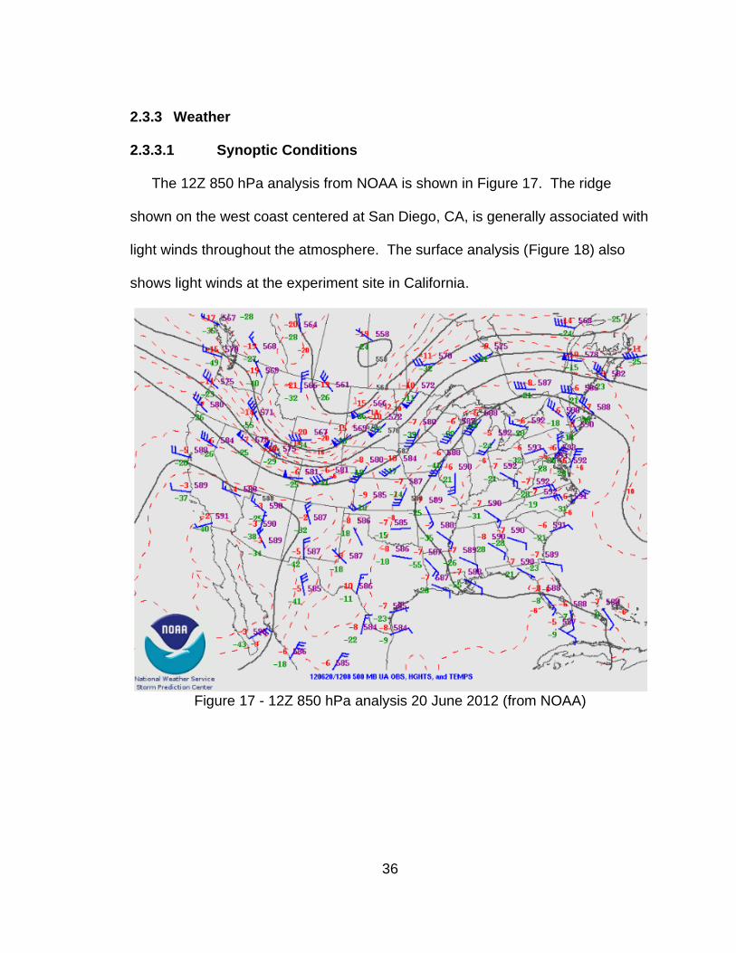
The 12Z 850 hPa analysis from NOAA is shown in Figure 17. The ridge

shown on the west coast centered at San Diego, CA, is generally associated with

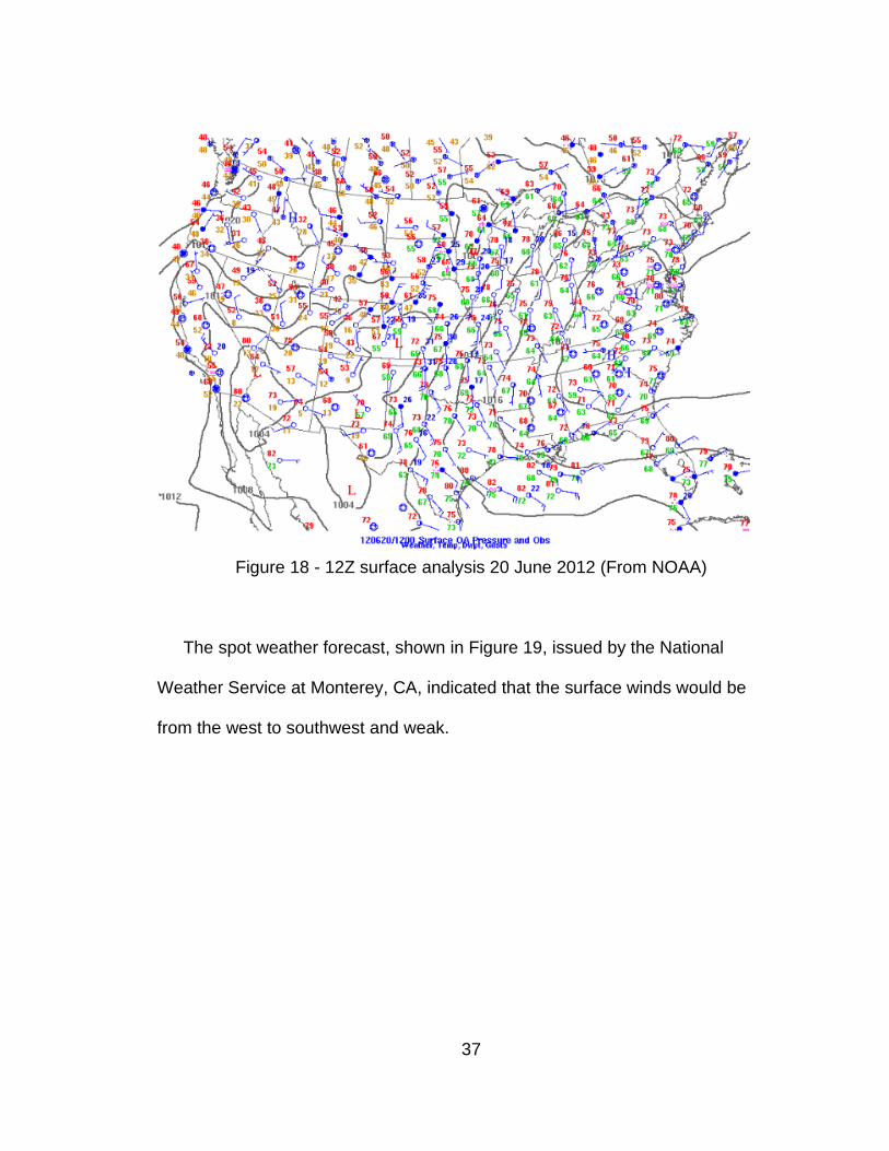
light winds throughout the atmosphere. The surface analysis (Figure 18) also

shows light winds at the experiment site in California.

Figure 17 - 12Z 850 hPa analysis 20 June 2012 (from NOAA)

37

Figure 18 - 12Z surface analysis 20 June 2012 (From NOAA)

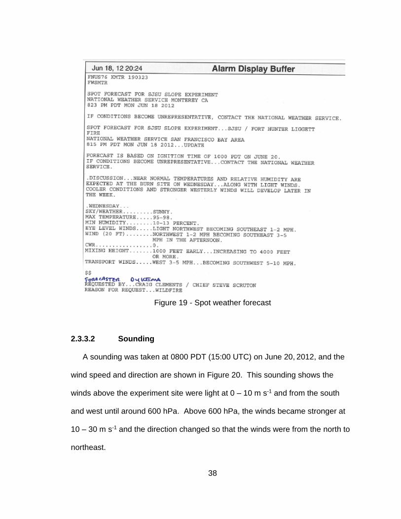
The spot weather forecast, shown in Figure 19, issued by the National

Weather Service at Monterey, CA, indicated that the surface winds would be

from the west to southwest and weak.

38

Figure 19 - Spot weather forecast

2.3.3.2 Sounding

A sounding was taken at 0800 PDT (15:00 UTC) on June 20, 2012, and the

wind speed and direction are shown in Figure 20. This sounding shows the

winds above the experiment site were light at 0 – 10 m s-1 and from the south

and west until around 600 hPa. Above 600 hPa, the winds became stronger at

10 – 30 m s-1 and the direction changed so that the winds were from the north to

northeast.

39

Figure 20 - Sounding wind speed (left) and direction (right)

The air temperature and dewpoint are shown in Figure 21. The separation of

the temperatures indicates dry conditions at all levels of the atmosphere, but very

dry conditions below 600 hPa.

Figure 21 - Sounding temperature and dew point

40

2.3.3.3 Sodar

The sodar profile (Figure 22) shows the winds were from the west around

0800 PDT (1500 UTC) and had shifted to from the north by 0900 PDT (1600

UTC). Prior to ignition at 11:18 PDT (1818 UTC), the winds were again shifting

and were from the east just after ignition. The wind speeds were very light both

prior to and after ignition. Ignition time is indicated by the red line.

Figure 22 - Sodar wind profile 20 June 2012

2.3.3.4 Lidar

The Lidar was located east of the experiment site (Figure 7). The wind was

analyzed at 0800 PDT (Figure 23) and 1119 PDT (Figure 24). Positive wind

velocities, shown as the greens, yellows, and reds for this experiment, indicate

wind from the east, blowing away from the Lidar. Negative wind velocities are

shown as turquoise to blue and indicate wind blowing from the west, from the

41

experiment site towards the Lidar. The RHI (Range Height Indicator) Lidar scan

prior to the experiment at 0832 PST (Figure 23) shows an easterly wind of 1 m s-

1 in a layer from the surface to around 200 m AGL (above Ground Level). The

winds above 300 m were more westerly with velocities closer to 2 m s-1. The

second scan, at the time of ignition, shows the upper-level winds had moved

lower in the atmosphere and the winds at the experiment site were mixed to

more westerly (Figure 24).

Figure 23 - Lidar RHI profile 08:32 PDT (1532 UTC) 20 June 2012

Figure 24 - Lidar at ignition 11:19 PDT (1919 UTC) 20 June 2012

42

2.3.3.5 AWS

The wind speed and direction are shown for the lower AWS in Figure 25.

Ignition time is indicated by the dotted line. The wind speed varied between 1 m

s-1 and 3.5 m s-1. This AWS was located on the ignition line. There was some

variation of the wind direction at the ignition line from east to west as the fire

progressed. At the time of ignition, the wind speed was 2.1 m s-1 and the wind

direction was 135o or from the SE and these values were later used in the

BehavePlus simulations.

It was discovered after the experiment that the upper AWS had not been

adequately secured and had moved some time after installation, so the data

could not be used.

Figure 25 - Lower AWS

43

2.3.3.6 Micromet Sonics

The wind speed and direction were measured at each of the 3 towers within

the experiment site. Tower 1 was the lowest on the slope and was designated as

bottom, Tower 2 was middle, and Tower 3 was top. These measurements are

shown in Figure 26. The ignition time is shown by the dotted line and the time

the fire front progressed through each tower is shown by the arrows. The wind

speed, in red, increased from 1 m s-1 to 9 m s-1 at Tower 1 (bottom) as the fire

front passed, but the wind decreased from 6 to 3 m s-1 as the fire front passed

Tower 2 (middle), and there was no change in wind speed as the fire front

passed Tower 3 (top). The wind direction was from the west (270o) at Tower 1

and Tower 2, but was from the east (90o) at Tower 3.

Figure 26 – 10 m wind speed and direction for the 3 towers

44

2.3.4 Fire Behavior

2.3.4.1 Fire Boundary Determination

The fire boundary was manually drawn on georeferenced images of the fire.

The fire was videoed from a helicopter overhead. The videos were processed in

Photoshop to collect images of the fire progression at regular time intervals.

These images were then georeferenced to the fire site using ArcGIS. The

process to collect and create these images is detailed below.

A helicopter flew above the fire and a video of the fire progression was

generated using a Canon Digital Video Recorder shooting at 30 frames per

second. The size of the video files prevented recording the video in one

complete segment. The first 25 minutes of the fire were recorded in 5 separate

video segments. In addition, several files were desired in case there was a

malfunction of the camera during the video capture. The video images were

recorded in high definition video MTS (MPEG (Moving Picture Experts Group)

Transport Stream) format. The last 10 – 15 minutes of the fire were not recorded

as the fire progression was so slow that little additional information would be

gained. The helicopter was released from the incident at that time. The

metadata for each of the 5 segments were obtained using ExifTool version 9.28

(Harvey 2013) and the results are shown in Table 10. These data were used to

calculate the precise frame needed in each video to show the fire activity at

desired increments. Please note that the times shown here are the metadata

times and not the GPS times.

45

Table 10 - Video Segment Metatdata Summary

Each video segment was imported into Adobe Photoshop CS6. Adobe

Photoshop CS6 allows manipulation of the video data so that the pixels in every

frame of the video may be examined. It was difficult to determine exactly which

frame was the first for the ignition of the fire since the distance of the helicopter

from the ignition point caused the fire ignition to be contained in only a small

number of pixels. However, by manually scanning the images for the first

appearance of pixels with the color of the flames, the video time for ignition was

determined to be 5 seconds after the start of the first video segment

(00005Ignition.mts). This corresponds with a recorded GPS ignition time of

11:18:10 PDT (19:19:10 UTC). Unfortunately, the video camera was never

synched to a GPS clock, so there may be a very small error in the times

associated with the video images. This is one limitation of the study.

Once the ignition time and frame were determined, the snapshot tool in

Photoshop was used to capture the image of the frame. This snapshot was then

saved in two formats: as a Photoshop file (.psd) for further pixel image analysis,

and as a tiff (Tagged Image File Format) for georeferencing.

Video File NameDate and Starting Time

from meta data

Start

TimeDuration

Calculated

Ending

Time

Gap Until

Next

Video

00005Ignition.MTS 2012:06:20 11:17:31-08:00 11:17:31 0:04:53.00 11:22:24.00 0:00:06.00

00006Tower1.MTS 2012:06:20 11:22:30-08:00 11:22:30 0:06:34.00 11:29:04.00 0:00:05.00

00007Tower1-2.MTS 2012:06:20 11:29:09-08:00 11:29:09 0:04:15.00 11:33:24.00 0:00:03.00

00008Tower2.MTS 2012:06:20 11:33:27-08:00 11:33:27 0:01:53.00 11:35:20.00 0:02:13.00

00009Tower2-3.MTS 2012:06:20 11:37:33-08:00 11:37:33 0:05:29.00 11:43:02.00

46

The video was then advanced exactly 30 seconds and new tiff and Photoshop

images were captured for that frame. This process was repeated until the end of

the video segment.

There were time gaps between the separate video segments. The metadata

were used to determine gap length so that the target time in the next segment for

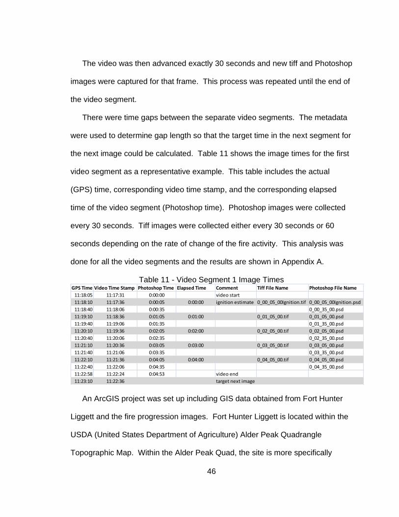
the next image could be calculated. Table 11 shows the image times for the first

video segment as a representative example. This table includes the actual

(GPS) time, corresponding video time stamp, and the corresponding elapsed

time of the video segment (Photoshop time). Photoshop images were collected

every 30 seconds. Tiff images were collected either every 30 seconds or 60

seconds depending on the rate of change of the fire activity. This analysis was

done for all the video segments and the results are shown in Appendix A.

Table 11 - Video Segment 1 Image Times

An ArcGIS project was set up including GIS data obtained from Fort Hunter

Liggett and the fire progression images. Fort Hunter Liggett is located within the

USDA (United States Department of Agriculture) Alder Peak Quadrangle

Topographic Map. Within the Alder Peak Quad, the site is more specifically

GPS Time Video Time Stamp Photoshop Time Elapsed Time Comment Tiff File Name Photoshop File Name

11:18:05 11:17:31 0:00:00 video start

11:18:10 11:17:36 0:00:05 0:00:00 ignition estimate 0_00_05_00Ignition.tif 0_00_05_00Ignition.psd

11:18:40 11:18:06 0:00:35 0_00_35_00.psd

11:19:10 11:18:36 0:01:05 0:01:00 0_01_05_00.tif 0_01_05_00.psd

11:19:40 11:19:06 0:01:35 0_01_35_00.psd

11:20:10 11:19:36 0:02:05 0:02:00 0_02_05_00.tif 0_02_05_00.psd

11:20:40 11:20:06 0:02:35 0_02_35_00.psd

11:21:10 11:20:36 0:03:05 0:03:00 0_03_05_00.tif 0_03_05_00.psd

11:21:40 11:21:06 0:03:35 0_03_35_00.psd

11:22:10 11:21:36 0:04:05 0:04:00 0_04_05_00.tif 0_04_05_00.psd

11:22:40 11:22:06 0:04:35 0_04_35_00.psd

11:22:58 11:22:24 0:04:53 video end

11:23:10 11:22:36 target next image

47

located within the North East Digital Ortho Quarter Quad (NE DOQQ). A digital

copy of the Alder Peak NE DOQQ was downloaded from the State of California

Geoportal and loaded as the initial layer into an ArcGIS project to establish the

UTM Zone 10N projection using the World Geodetic System (WGS) 1984 Datum.

Fort Hunter Liggett also provided a digital 5m contour map. During the setup of

the experiment, the GPS locations of the field instruments, other key markers,

and patches of differing vegetation were recorded. Each subset of information

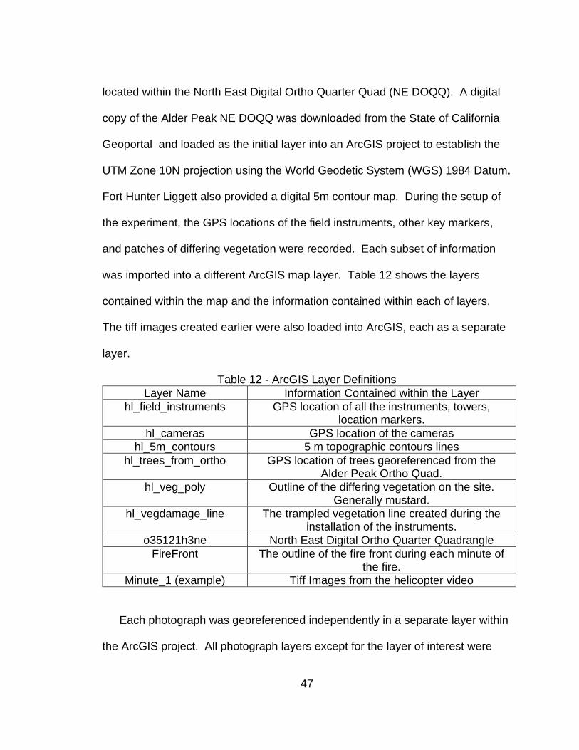
was imported into a different ArcGIS map layer. Table 12 shows the layers

contained within the map and the information contained within each of layers.

The tiff images created earlier were also loaded into ArcGIS, each as a separate

layer.

Table 12 - ArcGIS Layer Definitions

Layer Name Information Contained within the Layer

hl_field_instruments GPS location of all the instruments, towers, location markers.

hl_cameras GPS location of the cameras

hl_5m_contours 5 m topographic contours lines

hl_trees_from_ortho GPS location of trees georeferenced from the Alder Peak Ortho Quad.

hl_veg_poly Outline of the differing vegetation on the site. Generally mustard.

hl_vegdamage_line The trampled vegetation line created during the installation of the instruments.

o35121h3ne North East Digital Ortho Quarter Quadrangle

FireFront The outline of the fire front during each minute of the fire.

Minute_1 (example) Tiff Images from the helicopter video

Each photograph was georeferenced independently in a separate layer within

the ArcGIS project. All photograph layers except for the layer of interest were

48

turned off to isolate the layer of interest. The helicopter moved location during

the videotaping, so the viewing angles of the fire varied in the video. Therefore,

the same set of reference points could not be used to georeference every image.

Three to five points were selected to use for georeferencing for each image. The

points chosen depended on the location of the active fire line. This ensured that

the portion of the photograph containing the active fire was georeferenced

accurately. For example, two points on the ignition line and the first

meteorological tower were selected for the ignition image. As the fire moved up

the slope, different points were chosen based on where the fire front was located

and what points could be seen through the smoke.

Since the photos were at an oblique angle to the map, it was difficult to match

the photograph to the map exactly. Warping of the photo occurred inconsistently,

with some sections of the photograph warped slightly and some severely warped.

Generally with satellite photographs, the entire photograph is georeferenced to

minimize the Root Mean Square (RMS) error. However, only the fire section of

the photographs was of interest here, so the georeferencing points were selected

to have a good visual match at the area of interest (fire line) and RMS error was

ignored in this case. Minute 4 is shown, for example, in Figure 27, and the

georeferenced points are shown in Table 13. The complete list of georeference

points and the meaning for each reference point designation are given in

Appendix C.

49

Table 13 - Sample Georeference Points (Minute 4)

Original Image Georeferenced Image

Figure 27 - Sample georeferenced image (Minute 4)

Once the images had been georeferenced, the fire boundary line could then

be created. A separate, empty, shapefile (FireFront) for the fire boundaries was

created and added to the GIS project. This shapefile used the same coordinate

system as the other layers in the project. For each georeferenced photo of the

fire, a new map feature was created and saved in the FireFront shapefile. The

new feature was a polyline and was manually created by selecting points with the

Sketch tool along the visible portions of the fireline. Multiple points were used for

each polyline so that the fire boundary line had detail. The name attribute for

each polyline was edited to ensure the fire boundaries were associated with the

Photo Point #1

Description Layer

Point #2 Description

Layer

Point #3 Description

Layer

RMS Error

4 0_04_0

5_00

FID50 LoNRefPost

hl_field_instruments

FID2 Tower1

hl_field_instruments

FID5 Tower2

hl_field_instruments

0.00

50

correct minute of the fire. The fire boundary for minute four is shown as the black

line in Figure 28. All fire boundaries are shown in Figure 29. A table with the

original picture, the georeferenced picture, and the fire boundary for each minute

may be found in Appendix C.

Figure 28 - Fire boundary - shown as a black line for minute 4

51

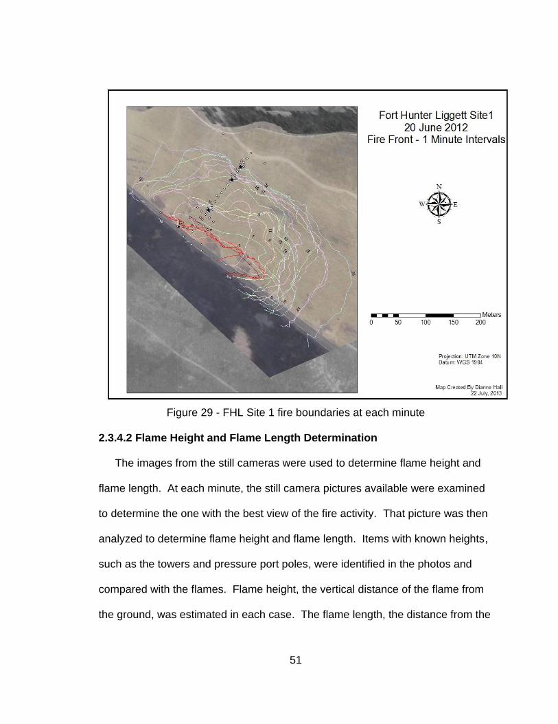
Figure 29 - FHL Site 1 fire boundaries at each minute

2.3.4.2 Flame Height and Flame Length Determination

The images from the still cameras were used to determine flame height and

flame length. At each minute, the still camera pictures available were examined

to determine the one with the best view of the fire activity. That picture was then

analyzed to determine flame height and flame length. Items with known heights,

such as the towers and pressure port poles, were identified in the photos and

compared with the flames. Flame height, the vertical distance of the flame from

the ground, was estimated in each case. The flame length, the distance from the

52

base of the flame to the tip of the flame, was also determined. Analysis at minute

six is shown in Figure 30 as a sample of the photo analysis technique.

Figure 30 - Sample flame height and length - minute 6

Key

Black flame height

Green flame length

Purple 10 ft pole for pressure ports

Red 10 m micrometeorological tower

Orange Rate of Spread markers (6ft)

Blue ft fence marker

2.3.4.3 Heat Flux

The radiative heating from the fire was measured using the radiometers on

each of the 10 m towers in the experiment site. For a detailed discussion of the

setup and analysis see Contezac (2019).

53

CHAPTER 3 Observed Fire Behavior

3.1 Rate of Spread (ROS)

To obtain the rate of spread at the fire front, the measurement tool was used

on the georeferenced pictures in ArcGIS. For the overall ROS (Show 1919), the

distance of the fire front from the ignition line was measured for each minute.

Since the ROS observed was not uniform, the ROS for each minute, the distance

from the fire front for the previous minute to the current minute, was also

measured. These calculations are shown in Table 14 and results presented in

Figure 31. Data were not available for every minute; however, the average ROS

over the fire experiment was 0.1 m s-1. The highest observed ROS were at

minute three of 0.4 m s-1 and at minute 16 of 0.5 m s-1. At minute three, the fire

was burning through the taller grass at the base of the slope and through the

mustard grass. The high ROS at minute 16 is inconsistent with the fire behavior

photographed at that minute. The helicopter changed positions at minute 17, so

the video perspective of the fire changed, and this affected the graphed

perimeter of the fire. Table 14 shows a negative progression of the fire for

minute 17. Since this is not possible, the method used to obtain the fire

perimeter and area may not be the best in this case.

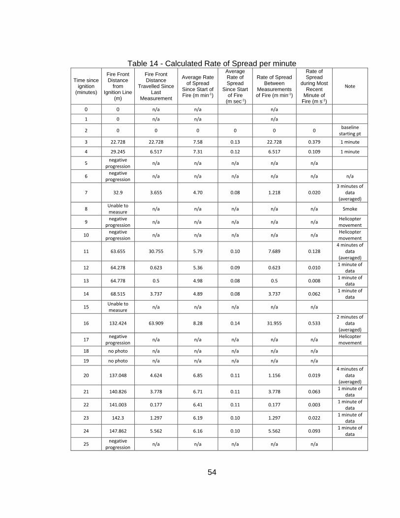
54

Table 14 - Calculated Rate of Spread per minute

Time since ignition

(minutes)

Fire Front Distance

from Ignition Line

(m)

Fire Front Distance

Travelled Since Last

Measurement

Average Rate of Spread

Since Start of Fire (m min-1)

Average Rate of Spread

Since Start of Fire

(m sec-1)

Rate of Spread Between

Measurements of Fire (m min-1)

Rate of Spread

during Most Recent

Minute of Fire (m s-1)

Note

0 0 n/a n/a n/a

1 0 n/a n/a n/a

2 0 0 0 0 0 0 baseline

starting pt

3 22.728 22.728 7.58 0.13 22.728 0.379 1 minute

4 29.245 6.517 7.31 0.12 6.517 0.109 1 minute

5 negative

progression n/a n/a n/a n/a n/a

6 negative

progression n/a n/a n/a n/a n/a n/a

7 32.9 3.655 4.70 0.08 1.218 0.020 3 minutes of

data (averaged)

8 Unable to measure

n/a n/a n/a n/a n/a Smoke

9 negative

progression n/a n/a n/a n/a n/a

Helicopter movement

10 negative

progression n/a n/a n/a n/a n/a

Helicopter movement

11 63.655 30.755 5.79 0.10 7.689 0.128 4 minutes of

data (averaged)

12 64.278 0.623 5.36 0.09 0.623 0.010 1 minute of

data

13 64.778 0.5 4.98 0.08 0.5 0.008 1 minute of

data

14 68.515 3.737 4.89 0.08 3.737 0.062 1 minute of

data

15 Unable to measure

n/a n/a n/a n/a n/a

16 132.424 63.909 8.28 0.14 31.955 0.533 2 minutes of

data (averaged)

17 negative

progression n/a n/a n/a n/a n/a

Helicopter movement

18 no photo n/a n/a n/a n/a n/a

19 no photo n/a n/a n/a n/a n/a

20 137.048 4.624 6.85 0.11 1.156 0.019 4 minutes of

data (averaged)

21 140.826 3.778 6.71 0.11 3.778 0.063 1 minute of

data

22 141.003 0.177 6.41 0.11 0.177 0.003 1 minute of

data

23 142.3 1.297 6.19 0.10 1.297 0.022 1 minute of

data

24 147.862 5.562 6.16 0.10 5.562 0.093 1 minute of

data

25 negative

progression n/a n/a n/a n/a n/a

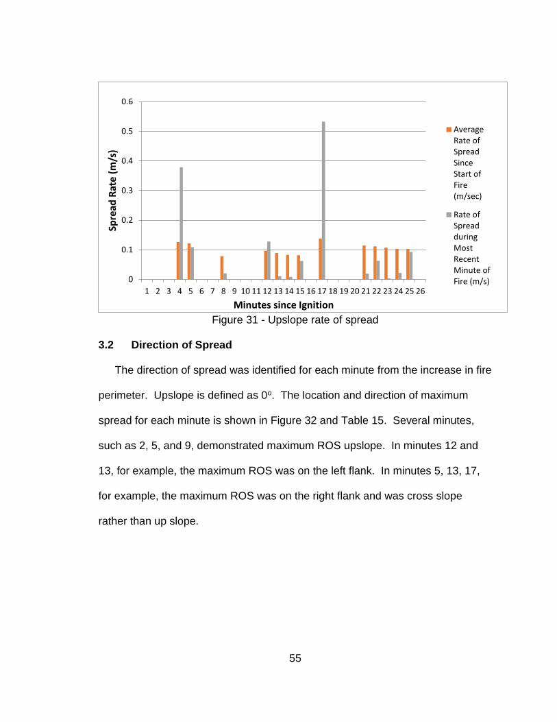
55

Figure 31 - Upslope rate of spread

3.2 Direction of Spread

The direction of spread was identified for each minute from the increase in fire

perimeter. Upslope is defined as 0o. The location and direction of maximum

spread for each minute is shown in Figure 32 and Table 15. Several minutes,

such as 2, 5, and 9, demonstrated maximum ROS upslope. In minutes 12 and

13, for example, the maximum ROS was on the left flank. In minutes 5, 13, 17,

for example, the maximum ROS was on the right flank and was cross slope

rather than up slope.

0

0.1

0.2

0.3

0.4

0.5

0.6

1 2 3 4 5 6 7 8 9 10 11 12 13 14 15 16 17 18 19 20 21 22 23 24 25 26

Spre

ad R

ate

(m/s

)

Minutes since Ignition

AverageRate ofSpreadSinceStart ofFire(m/sec)

Rate ofSpreadduringMostRecentMinute ofFire (m/s)

56

Table 15 - Direction of Maximum Fire Spread (in degrees)

Minute Since Ignition Direction of Maximum Fire Spread in degrees (0o is upslope)

2 0

3 110

4 30

5-1 0

5-2 105

6 0

7 0

9-1 40

9-2 0

11 0

12 310

13 300

13-2 80

14 30

15 30

16 0

17-1 65

17-2 0

17-3 310

20 310

21 280

22 0

23 0

24 300

57

Figure 32 - Location of maximum fire rate of spread at each minute

3.3 Flame Length, Flame Height, Flame Angle

The observed flame heights, flame lengths and flame angles are given in

Table 16 below. The flame angle is given from the vertical. When the flame

angle is 0o, then the flame is not influenced by wind. This is the case for minutes

0-3. At minutes 4 through 12 there is a flame angle indicating that the flames

were being influenced by wind. From Minute 13 the flame angle was 0 o,

indicating that the flame was no longer under the influence of wind. The largest

58

flame angle occurred at minutes 4 and 5 which is consistent with the increase in

wind (Figure 25).

Table 16 – Observed Flame Height, Length, and Angle at Each Minute

Minute Flame Height (m) Flame Length (m) Flame Angle

0 0.7 0.7 0

1 1 – 1.5 1 – 1.5 0

2 0.5 – 1.0 0.75 – 1.5 0

3 0.5 – 1.0 0.5 -1.0 0

4 0.1 – 0.3 0.1 – 0.3 45

5 0.5 – 1.0 0.5 – 1.0 45

6 0.5 – 1.0 0.5 – 1.0 30

7 1.5 - 4.0 1.5 – 4.5 15

8 1.0 – 3.0 1.0 – 3.0 15

9 1.0 – 4.0 1.0 – 4.0 30

10 0.5 – 1.0 0.5 – 1.0 15

11 0.25 – 0.5 0.25 – 0.5 0

12 0.25 – 0.5 0.25 – 0.5 30

13 No picture available No picture available -

14 2.0 – 5.0 2.0 – 5.0 0

15 2.0 2.0 0

16 1.0 - 3.0 1.0 – 3.0 0

17 No picture available No picture available -

18 0.5 - 2.0 0.5 – 2.0 0

19 0.5 – 1.0 0.5 – 1.2 0

20 0.25 – 2.0 0.25 – 2.0 0

21 No picture available No picture available -

22 No picture available No picture available -

23 No picture available No picture available -

24 No picture available No picture available -

25 0.25 – 0.5 0.25 – 0.5 0

3.4 Fire Perimeter and Fire Area

After the creation of the fire line, the length of the fire line perimeter and the

area of the fire were measured using the georectified photos in ArcGIS as

detailed previously. The values are given in Table 17 and are graphed in Figure

33 (perimeter) and Figure 34 (area). The apparent reduction in fire area at

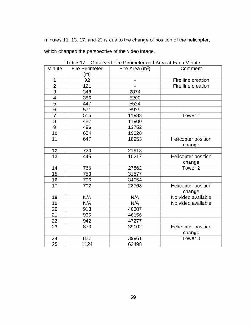
59

minutes 11, 13, 17, and 23 is due to the change of position of the helicopter,

which changed the perspective of the video image.

Table 17 – Observed Fire Perimeter and Area at Each Minute

Minute Fire Perimeter (m)

Fire Area (m2) Comment

1 92 - Fire line creation

2 121 - Fire line creation

3 348 2874

4 386 5200

5 447 5524

6 571 8929

7 515 11933 Tower 1

8 487 11900

9 486 13752

10 654 19028

11 647 18953 Helicopter position change

12 720 21918

13 445 10217 Helicopter position change

14 766 27562 Tower 2

15 753 31577

16 796 34054

17 702 28768 Helicopter position change

18 N/A N/A No video available

19 N/A N/A No video available

20 913 40307

21 935 46156

22 942 47277

23 873 39102 Helicopter position change

24 827 39961 Tower 3

25 1124 62498

60

Figure 33 - Fire perimeter

Figure 34 - Fire area

0

200

400

600

800

1000

1200

1 2 3 4 5 6 7 8 9 10 11 12 13 14 15 16 17 18 19 20 21 22 23 24 25

Per

imet

er L

engt

h (

m)

Minutes Since Ignition

0

10000

20000

30000

40000

50000

60000

70000

1 2 3 4 5 6 7 8 9 10 11 12 13 14 15 16 17 18 19 20 21 22 23 24 25

Fire

Are

a (m

2 )

Minutes Since Ignition

61

CHAPTER 4 Analysis of Fire Behavior

4.1 Fire Behavior Prediction (BehavePlus)

The software BehavePlus was used to predict the fire behavior as mentioned

earlier. Due to the slope change from 15% (9o) to 30% (17o) at Tower 1, the runs

were separated into Ignition to Tower 1 and Tower 1 to Tower 3. The input and

output data of the BehavePlus runs from Ignition to Tower 1 are shown in Table

18 and for Tower 1 to Tower 3 in Table 19. The rate of spread and flame length

predicted for this fire are classified as low (Scott and Burgan 2005).

Table 18 - BehavePlus Fire Prediction for Ignition to Tower 1

Inputs

Fuel Model GR4 GR4 3

1HR Moisture 1.6% 2.25% 3%

Midflame Wind Speed 7.7 km hr-1 7.7 km hr-1 7.7 km hr-1

Wind Direction (from N) 128o 128o 128o

Air Temperature 33.3 oC 33.3 oC 33.3 oC

Fuel Shading 0% 0% 0%

Slope 15% 15% 15%

Aspect 225o 225o 225o

Spread Direction 45o 45o 45o

Elapsed Time 0.133hr

(7 minutes) 0.133hr

(7 minutes) 0.133hr

(7 minutes)

Outputs

Surface Rate of Spread (m min-1)

0.9 0.8 5.1

Fireline Intensity (kW m-1)

66 48 878

Flame Length (m) 0.5 0.5 1.7

Reaction Intensity (kW m2)

346 298 666

Surface Spread Distance (m)

6.3 5.4 41.1

Area (m2) 2,000 1,000 65,000

Perimeter (m) 155 56.2 1009

62

Table 19 - BehavePlus Fire Prediction for Tower 1 to Tower 3

Inputs

Fuel Model GR4 GR4 3

1HR Moisture 1.6% 2.25% 3

Midflame Wind Speed 7.7 km hr-1 7.7 km hr-1 7.7 km hr-1

Wind Direction (from N) 128o 128o 128o

Air Temperature 33.3 oC 33.3 oC 33.3 oC

Fuel Shading 0% 0% 0%

Slope 30% 30% 30%

Aspect 225o 225o 225o

Spread Direction 45 o 45 o 45 o

Elapsed Time 0.28hr

(17 minutes) 0.28hr

(17 minutes) 0.28hr

(17 minutes)

Outputs

Surface Rate of Spread (m min-1)

1.0 0.9 5.6

Fireline Intensity (kW m-1)

72 53 958

Flame Length (m) 0.6 0.5 1.8

Reaction Intensity (kW m2)

346 298 666

Surface Spread Distance (m)

16.9 14.5 94.4

Area (m2) *9,000 *7,000 *287,000

Perimeter (m) *376 *322 *2118

Note that the area and perimeter for the second run of the model, from Tower

1 to Tower 3, assume a point source for the ignition at Tower 1. Since this is not

the case, the area and perimeter given at the end of the second BehavePlus run

would not be the predicted area and perimeter of the entire fire, just the new

section of the fire from Tower 1 to Tower 3. The total perimeter can be estimated

by adding the perimeters of the two runs, as can the total area be estimated by

adding the areas of the two runs.

63

4.2 Observed vs. Predicted Fire Behavior

The fire reached Tower 1 at minute seven of the fire, with an observed

average rate of spread from ignition of 4.7 m min-1. This was far faster than the

rate of 0.9 m min-1 predicted when using the GR4 fuel model at the lower fuel

moisture. Fuel Model 3 more closely represented the taller grass observed in the

initial part of the slope as shown in Figure 16. When using Fuel Model 3, the

predicted rate of spread was 5.1 m min-1, and this more closely approximated the

observed fire rate of spread.

Tower 3 was reached at minute 25 of the fire. Data were not available for

minute 25, but at minute 24 the average rate of spread from Tower 1 to Tower 3

was 6.16 m min-1, which was slightly above the predicted 5.6 m min-1 (FM3), but

far above the predicted 1 m min-1 (GR4). However, this average is skewed by

the 31.9 m min-1 ROS observed at minute 16. The rates of spread varied

between 0.1 m min-1 and 6 m min-1, which on the lower end match the GR4

prediction, while on the higher end match the FM3 prediction.

The observed perimeter of the fire at minute seven was 515 m, which was

below the perimeter of 1009 m predicted by FM3, but above the 155m predicted

by GR4. The observed perimeter at minute 25 was 1124 m, which was below

the estimate value of 3127 m (FM3), but again above the estimate of 531 m

(GR4).

The observed area of the fire at minute seven was 11933 m2, which was

below the predicated area of 65,000 m2 (FM3), and well below the area predicted

64

for GR4. The observed area of the fire at minute 25 was 62498 m2, which was

well below the area predicted by both models.

The observed flame lengths were close to the predicted flame lengths of 0.6

m (GR4) and 1.8 m (FM3), except for minutes seven to nine when the observed

flame lengths exceeded the predictions. The sonic anemometer on Tower 1

recorded an increase of wind speed at that time (Figure 26). The BehavePlus

runs used a wind speed of 7.7 km hr-1 (2 m s-1) obtained from the AWS at the

ignition line. However, the sonic anemometers show that the wind was not

steady during the fire and wind speeds actually varied from 0 to 9 m s-1.

Flame heights and flame angles were not predicted by BehavePlus, so

cannot be compared with the observations.

The experiment can be divided into 2 distinct sections. The first section was

from ignition to Tower 1. In this section, the slope was 15%, the most

appropriate fuel model was FM3, and the winds were at 45o from upslope.

During this portion of the experiment, the fire behavior was close to the predicted

values. The second section was from Tower 1 to Tower 3. In this section the

slope increased to 30%, the most appropriate fuel model was GR4, and the

winds had become downslope. During this portion of the experiment, the fire

behavior was much less than expected and occasional backing fire behavior was

observed

65

CHAPTER 5 Summary, Conclusions, Limitations of Study, Further Research

5.1 Summary

A headfire burned up a grass slope that had been instrumented in situ and

remotely. Both photographic and video images of the fire were captured. The

data from the instruments and the images were analyzed to determine the fire

behavior.

The original fuel model selected for the BehavePlus simulation was Fuel

Model 3 (FM3). After the fuel beds were analyzed, Grass Group 4 (GR4)

appeared to be the best selection. However, when both simulations were run

and compared with observed fire behavior, FM3 predicted more intense fire

behavior than was observed, while GR4 predicted less intense fire behavior.

The site selected for the fire was subject to prescribed burns each spring.

The fire department even expressed surprise at the slow rate of burn for this fire.

The original prediction was for a 12-minute burn duration from ignition to Tower

3. During the experiment the fire took almost 25 minutes to reach Tower 3. The

forward progression was slowed due to unexpected surfacing of the upper level

winds during the experiment, as shown in Figure 24. The winds changed from

upslope to downslope during this surfacing, and the fire became wind-driven

rather than slope-driven. The head of the fire became a backing fire during this

wind reversal. This resulted in a smaller perimeter and area for the fire than

predicted by FM3.

66

Since the wind was not in alignment with the slope, the fire burned across the

slope. This meant that the ignition for the fire could not be a point, but had to be

a line to ensure that the fire burned through the instrument towers. BehavePlus

assumes a point of origin for fires so this may have affected our results.

The flame lengths and flame heights varied from 0.5 to 4 m. This was within

the expected fire behavior. The most intense fire burned when the fire reached

Tower 1. This was when the wind reversal was occurring.

5.2 Conclusions

At the start of the experiment, the wind and slope were in alignment so that

the forward rate of spread was upslope / upwind. Wind and slope were

complementary contributors to the fire behavior. The fire burned upslope and

exhibited expected fire behavior with respect to rates of spread and flame

lengths. This behavior continued until Tower 1 was reached.

At Tower 1, the slope increased so an increase in the rate of spread was

predicted. The fuel load decreased so the flame lengths were expected to

decrease slightly. However, a wind reversal also occurred as the fire reached

Tower 1.

After the wind reversal, the slope and wind were in opposition with the wind

driving the fire downslope and the slope driving the fire upslope. The forward

progression of the fire slowed between Tower 1 and Tower 3, and the flame

lengths were reduced to less than 1 m. At times, backing fire behavior was

observed when the force of the wind overcame the force of the slope.

67

From this experiment, we can conclude that the wind speed and direction can

overcome the influence of slope on fire behavior. This has implications for

firefighter safety on wildland fires as fire is generally assumed to progress

upslope. If the wind overcomes the influence of the slope, and the fire

progression changes direction, then firefighters may find themselves in the path

of the fire. It is important that the vertical wind profile on an incident be

understood, not just the surface level winds, so that the potential for upper level

winds to surface may be considered in firefighter response planning.

5.3 Limitations of the Study

There were several limitations to this study. The video camera used in the

helicopter was not synced to a GPS clock, so exact ignition time was difficult to

determine. The smoke from the fire obscured the fire line. It was difficult to

determine precise fire boundary. The helicopter moved to different locations to

try to observe the fire line through the smoke. This changed the georeferencing

points for the photographs, so the fire perimeter estimation was not consistent.

At times the fire boundary appeared to shrink as time progressed. The infrared

camera that was supposed to be used in the helicopter malfunctioned, so the fire

perimeters could not be obtained using that instrument. The laboratory oven

malfunctioned when drying fuel moisture samples, destroying most of the

samples, so the fuel moisture content was an estimate. The flame heights were

difficult to measure as there were no height markers placed within the experiment

plot. The rate of spread markers were difficult to see through the smoke and

68

were not in line with the fire progression, so they could not be used to estimate

the rate of spread.

Additionally, BehavePlus is generally used to predict fire behavior over longer

periods of time, such as hours or days rather than minutes. It is also generally

used for much larger geographic areas. BehavePlus assumes an average

constant wind speed for making its predictions, which is appropriate for long

durations, but there were several wind speed and direction changes during the

25-minute experiment run.

The planned ignition was for earlier in the day when conditions are generally

calmer; however, there were several logistical delays on the day of the fire which

pushed out the start. This meant dryer fuels and exposure to surfacing winds.

5.4 Further Research / Next Steps

Since the experiment site is subject to annual prescribed burns, it would be

useful to collect information on subsequent burns. The fire behavior could be

observed using Lidar and video only rather than the entire instrument suite used

in this experiment. This would enable comparison of the fire behavior from this

experiment with fire behavior when the winds do not surface.

To better understand the behavior of fire on slopes, a longer duration fire

should be studied which would require a longer slope. Again, remote

instruments such as Lidar and videographic recordings would gather much of the

information needed to analyze the fire behavior. Once fire behavior on grass

69

slopes is understood, then the same experiment should be run in different fuel

types, such as California chaparral or brush.

Acknowledgements

The members of the Fire Weather Research Lab contributed greatly to this

experiment. The following figures listed in Table 20 used in this thesis were

created by other members of the Fire Weather Research Lab team as indicated

and are used with permission. The Biomass fuel loading calculations were

performed by a team from the US Forest Service Pacific Northwest Wildland Fire

Science Laboratory and are used with permission.

Table 20 - Figures created by team members

Figure/Table Created By

Figure 22 - Sodar wind profile 20 June 2012 Jon Contezac

Figure 23 - Lidar RHI profile 08:32 PDT (1532 UTC) 20 June 2012

Allison Charland Bagley

Figure 24 - Lidar at ignition 11:19 PDT (1919 UTC) 20 June 2012

Allison Charland Bagley

GIS of the experiment plot and ArcGIS setup Braniff Davis

Table 9 - Biomass Fuel Loading Fort Hunter Liggett Site 1

US Forest Service Pacific Northwest Research Station, Pacific Wildland Fire Sciences Laboratory

70

References

Albini, Frank A. 1976. Estimating wildfire behavior and effects. USDA For. Serv. Gen. Tech. Rep. INT-30, 92 pp, Inter-mountain Forest and Range Experiment Station, Ogden, Utah 84401. https://www.fs.fed.us/rm/pubs_int/int_gtr030.pdf

American Meteorological Society, cited 2019: "Weather”. Glossary of Meteorology. [Available online at http://glossary.ametsoc.org/wiki/Weather]

Anderson, H., Brackebusch, A., Mutch, R., and Rothermel, R., 1966: Mechanisms of Fire Spread, Research Progress Report 2 - INT-28. 35pp, Ogden, Utah: USDA Forest Service, Intermountain Forest and Range Experiment Station. https://www.fs.fed.us/rm/pubs_exp_for/priest_river/exp_for_priest_river_1966_anderson.pdf

Anderson, Hal E.1982. Aids to determining fuel models for estimating fire behavior. USDA Forest Service General Technical Report INT-122, 22 pp, lntermountain. Forest and Range Experimental Station., Ogden,Utah 8440. https://www.fs.fed.us/rm/pubs_int/int_gtr122.pdf

Anderson, W., Pastor, E., Butler, C., Catchpole, E., Dupuy J-L, Fernandes, P., Ventura, J., 2006: Evaluating Models to estimate flame characteristics for free-burning fires using laboratory and field data. Forest Ecology and Management, 1-19.

Andrews, P.L., C.D. Bevins, and R.C. Seli. 2005: BehavePlus fire modeling system version 3.0 user’s guide. 153 pp, USDA Forest Service General Technical Report RMRS-GTR-106. https://www.frames.gov/documents/behaveplus/publications/Andrews_Bevins_Seli_2004_RMRS-GTR-DRAFT.pdf

Beer, T.,1993: The speed of a fire front and its dependence on wind speed. International Journal of Wildland Fire, 3, 193-202.

Bird, R. B., Stewart, W. E., and Lightfoot, E. N., 1960: Transport Phenomena. Wiley. 780 pp.

Butler, B. W., 2014: Wildland firefighter safety zones: a review of past science and summary of future needs. International Journal of Wildland Fire, 23, 295-308

Byram, G. M., 1959: Chapter 3 - Combustion of Forest Fire Fuels, Forest Fire: Control and Use, K. P. Davis, McGraw-Hill, 61-89

71

CA GOV. 2013: April 29. Retrieved from The State of California Geoportal: http://portal.gis.ca.gov/geoportal/catalog/main/home.page

Clements, C. B., 2006: In situ measurements of water vapor, heat, and CO2 fluxes within a prescribed grass fire. International Journal of Wildland Fire, 15, 299-306.

Clements, C. B., 2007: Observing the Dynamics of Wildland Grass Fires. FireFlux - A Field Validation Experiment. Bulletin of the American Meteorological Society, 1370-1382. https://doi.org/10.1175/BAMS-88-9-1369

Clements, C. B., 2008: First observations of turbulence generated by grass fires. Journal of Geophysical Research, 113, 1-13, https://doi.org/10.1029/2008JD010014

Clements, C.B. and Coauthors, 2014: Overview of the 2013 FireFlux II grass fire field experiment. In: Viegas, D.X., ed. Advances in Forest Fire Research. Coimbra, Portugal: Coimbra University Press: 392-400.

Clements, C. B. and A. Oliphant 2014: The California State University Mobile Atmospheric Profiling System: A facility for research and education in boundary-layer meteorology. Bulletin of the American Meteorological Society, 95, 1713–1724.

Clements, C. B., and Seto, D., 2015: Observations of Fire-Atmosphere Interactions and Near-Surface Heat Transport on a Slope. Boundary-Layer Meteorology, 154, 409-426.

Clements C. B., and Coauthors, 2019: The FireFlux II experiment: a model-guided field experiment to improve understanding of fire–atmosphere interactions and fire spread. International Journal of Wildland Fire 28 308-326.

Contezac, J. M., 2018: Micrometeorological Observations of Fire-Atmosphere Interactions and Fire Behavior on a Simple Slope, Master’s Thesis.

Covele, 2008: Wildland Toolkit. Peakview Software LLC https://apps.apple.com/us/app/wildland-toolkit/id318683999

Curry, J., and Fons, W., 1938: Rate of spread of surface fires in the ponderosa pine type of California. Journal of Agricultural Research, 57, 239-267.

Curry, J., and Fons, W., 1940: Forest-fire behavior studies. Mechanical Engineering, 62, 219-225.

72

Dold, J., Simeoni, A., Zinoviev, A, and Weber, R, 2009:The Palasca Fire, September 2000: Eruption or Flashover?, Recent Forest Fire Related Accidents in Europe, Viegas D. X., 82 pp, Joint Research Centre, Institute for Environment and Sustainability EUR 24121 EN – 2009, 54-64. https://effis.jrc.ec.europa.eu/media/filer_public/6c/70/6c70555f-4b0c-47f7-b649-4c3fa4e1e9f9/recent-forest-fire-related-accidents-in-europe_ec3ybmu.pdf

Dupuy, J. L., Maréchal, J., Portier, D. and Valette, J.-C., 2011: The effects of slope and fuel bed width on laboratory fire behaviour. International Journal of Wildland Fire, 20, 272-288. https://doi.org/10.1071/WF09075

Fons, W. L., 1946: Analysis of Fire Spread in Light Forest Fuels. Journal of Agricultural Research, 72, 93-121.

Frandsen, W. H., 1971: Fire Spread through Porous Fuels from the Conservation of Energy. Combustion and Flame, 16, 9-16.

Gray, L. G., 1933: Preliminary Report on Fire Hazard Rating Study. San Francisco: U. S. Weather Bureau.

Hardy, C.E., 1977: The Gisborne Era of Forest Fire Research. 6pp, Missoula, MT: University of Montana, Forest and Conservation Experiment Station Completion Report Contract No. 12-11-204-1. https://www.nifc.gov/safety/mann_gulch/long_term_impacts/documents/FS-367_The_Gisborne_Era_of_Forest_Fire_Research_1949.pdf

Harvey, P., 2013, May 06: ExifTool by Phil Harvey. Retrieved from http://www.sno.phy.queensu.ca/~phil/exiftool/

IFSTA., 2013: Chapter 5 - Fire Behavior. Essentials of Firefighting, 6th Edition Fire Protection Publications. pp 1400

Keeley, J. E., 2009: Fire Intensity, fire severity and burn severity: a brief review and suggested usage. International Journal of Wildland Fire. 18, 116-126.

Linn, R. R., 2010: A numerical study of slope and fuel structure effects on coupled wildfire behaviour. International Journal of Wildland Fire. 19, 179-201.

MacLean, N., 1992: Young Men and Fire. Chicago: University of Chicago Press. pp 301.

73

McArthur, A. G., 1966: Weather and grassland fire behaviour. Canberra, Australia: Department of National Development, Forestry and Timber Bureau Leaflet No. 100.

McArthur, A. G., 1967: Fire behaviour in Eucalypt forests. Canberra, Commonwealth of Australia, Dept. of National Development, Forestry and Timber Bureau.

McArthur, A. G., 1969: The Tasmanian brushfires of 7th February, 1967 and associated fire behaviour characteristics. Mass Fire Symposium Proceedings. Maribyrnong, Victoria: Defense Standards Lab. p. 23

Mendes-Lopes, J. M., Ventura, J. M. P., and Amaral, J. M. P., 2003: Flame characteristics, temperature–time curves, and rate of spread in fires propagating in a bed of Pinus pinaster needles. International Journal of Wildland Fire, 12, 67-84.

Nelson, R. M. Jr, and Adkins, C. W., 1988: A dimensionless correlation for the spread of wind-driven fires. Canadian Journal of Forest Research, 18(4), 391-397. https://doi.org/10.1139/x88-058

NWCG, 1996: S-190 - Introduction to Wildland Fire Behavior. National Wildfire Coordination Group (NWCG). Retrieved from National Wildfire Coordinating Group: http://www.nwcg.gov/?q=glossary

Ottmar, R. D., and Coauthors, 2016: Measurements, datasets and preliminary results from the RxCADRE project - 2008, 2011 and 2012. International Journal of Wildland Fire, 25, 1-9 DOI: https://doi.org/10.1071/WF14161

Papadopoulos, G. D., and Pavlidou, F.-N., 2011: A Comparative Review on Wildfire Simulators. IEEE Systems Journal, 5, 233-243.

Potter, B., 2012a: Atmospheric interactions with wildland fire behaviour – I. Basic surface interactions, vertical profiles and synoptic structures. International Journal of Wildland Fire, 21, 779-801.

Rothermel, R., and Anderson, H., 1966: Fire Spread Characteristics determined in the laboratory – INT-30, 41 pp, Ogden, Utah: USDA Forest Service Intermountain Forest and Range Experimental Station. https://www.fs.fed.us/rm/pubs_int/int_rp030.pdf

Rothermel, R. C., 1972: A Mathematical Model for Predicting Fire Spread in Wildland Fuels (INT-115). 48pp Ogden, Utah: USDA Forest Service, Intermountain Forest and Range Experiment Station.

74

Schlobohm, P. B., 2002: Gaining an Understanding of the National Fire Danger Rating System (PMS 932 NFES 2665). National Wildfire Coordinating Group.

Scott, J. H., and Burgan, R. E., 2005: Standard Fire Behavior Fuel Models: A Comprehensive Set for Use with Rothermel’s Surface Fire Spread Model. 80pp, United States Forest Service, United States Department of Agriculture. Fort Colins, CO: Rocky Mountain Research Station. https://www.fs.fed.us/rm/pubs/rmrs_gtr153.pdf

Show, S., 1919: Climate and Forest Fires in Northern California. Journal of Forestry, 17, 965 - 979. https://doi.org/10.1093/jof/17.8.965

Thomas, P., 1967: Some aspects of the growth and spread of fire in the open. Forestry, 40, 139-164.

Thomas, P., 1971: Rates of Spread of some wind-driven fires. Forestry, 44, 155-175.

Weise, D. B., 1996: Effects of wind velocity and slope on flame properties. Can J. For. Res., 26, 1849-1858.

Weise, D. R., 1997: A Qualitative Comparison of Fire Spread Models Incorporating Wind and slope Effects. Forest Science, 43, 170-180.

Werth, P. A., and Coauthors, 2011: Synthesis of Knowledge of Extreme Fire Behavior: Volume 1 for Fire Managers., 144 pp, Gen. Tech. Rep. PNW-GTR-854. Portland, Oregon: US Department of Agriculture, Forest Service, Pacific Northwest Research Station. DOI: https://doi.org/10.2737/PNW-GTR-854

Wilson, C. C., 1977: Fatal and near-fatal forest fires: the common denominators. The International Fire Chief, 43, 9-10, 12-15.

Wolff, M. F., 1991: Wind-aided firespread across arrays of discrete fuel elements. II. Experiment. Combustion Science and Technology, 77, 261-289.

Wu, Y., Xing, H., and Atkinson, G., 2000: Interaction of Fire Plume with inclined surface. Fire Safety Journal, 35, 391-403. https://doi.org/10.1016/S0379-7112(00)00032-1

75

Appendix A – Video Segment Metadata

Video Segment Metadata summary

Video Segment 1 Times

Video Segment 2 Times

Video File NameDate and Starting Time

from meta data

Start

TimeDuration

Calculated

Ending

Time

Gap Until

Next

Video

00005Ignition.MTS 2012:06:20 11:17:31-08:00 11:17:31 0:04:53.00 11:22:24.00 0:00:06.00

00006Tower1.MTS 2012:06:20 11:22:30-08:00 11:22:30 0:06:34.00 11:29:04.00 0:00:05.00

00007Tower1-2.MTS 2012:06:20 11:29:09-08:00 11:29:09 0:04:15.00 11:33:24.00 0:00:03.00

00008Tower2.MTS 2012:06:20 11:33:27-08:00 11:33:27 0:01:53.00 11:35:20.00 0:02:13.00

00009Tower2-3.MTS 2012:06:20 11:37:33-08:00 11:37:33 0:05:29.00 11:43:02.00

GPS Time Video Time Stamp Photoshop Time Elapsed Time Comment Tiff File Name Photoshop File Name

11:18:05 11:17:31 0:00:00 video start

11:18:10 11:17:36 0:00:05 0:00:00 ignition estimate 0_00_05_00Ignition.tif 0_00_05_00Ignition.psd

11:18:40 11:18:06 0:00:35 0_00_35_00.psd

11:19:10 11:18:36 0:01:05 0:01:00 0_01_05_00.tif 0_01_05_00.psd

11:19:40 11:19:06 0:01:35 0_01_35_00.psd

11:20:10 11:19:36 0:02:05 0:02:00 0_02_05_00.tif 0_02_05_00.psd

11:20:40 11:20:06 0:02:35 0_02_35_00.psd

11:21:10 11:20:36 0:03:05 0:03:00 0_03_05_00.tif 0_03_05_00.psd

11:21:40 11:21:06 0:03:35 0_03_35_00.psd

11:22:10 11:21:36 0:04:05 0:04:00 0_04_05_00.tif 0_04_05_00.psd

11:22:40 11:22:06 0:04:35 0_04_35_00.psd

11:22:58 11:22:24 0:04:53 video end

11:23:10 11:22:36 target next image

GPS Time Video Time Stamp Photoshop Time Elapsed Time Comment Tiff File Name Photoshop File Name

11:23:04 11:22:30 0:00:00 video start after 6 sec pause

11:23:10 11:22:36 0:00:06 0:05:00 target image time 6-0_00_06_00.tif 6-0_00_06_00.psd

11:23:40 11:23:06 0:00:36 6-0_00_36_00.tif 6-0_00_36_00.psd

11:24:10 11:23:36 0:01:06 0:06:00 6-0_01_06_00.tif 6-0_01_06_00.psd

11:24:40 11:24:06 0:01:36 6-0_01_36_00.tif 6-0_01_36_00.psd

11:25:10 11:24:36 0:02:06 0:07:00 6-0_02_06_00.tif 6-0_02_06_00.psd

11:25:40 11:25:06 0:02:36 6-0_02_36_00.tif 6-0_02_36_00.psd

11:26:10 11:25:36 0:03:06 0:08:00 6-0_03_06_00.tif 6-0_03_06_00.psd

11:26:40 11:26:06 0:03:36 6-0_03_36_00.tif 6-0_03_36_00.psd

11:27:10 11:26:36 0:04:06 0:09:00 6-0_04_06_00.tif 6-0_04_06_00.psd

11:27:40 11:27:06 0:04:36 6-0_04_36_00.tif 6-0_04_36_00.psd

11:28:10 11:27:36 0:05:06 0:10:00 6-0_05_06_00.tif 6-0_05_06_00.psd

11:28:40 11:28:06 0:05:36 6-0_05_36_00.tif 6-0_05_36_00.psd

11:29:10 11:28:36 0:06:06 0:11:00 6-0_06_06_00.tif 6-0_06_06_00.psd

11:29:38 11:29:04 0:06:34 video end 6-0_06_34_11.tif 6-0_06_34_11.psd

11:29:40 11:29:06 0:11:30 target next image

76

Video Segment 3 Times

Video Segment 4 Times

Video Segment 5 Times

GPS Time Video Time Stamp Photoshop Time Elapsed Time Comment TIFF File name Photoshop File Name

11:29:43 11:29:09 0:00:00 video start after 5 sec pause

11:30:10 11:29:36 0:00:27 0:12:00 target image time 7-0_00_27_00.tif 7-0_00_27_00.psd

11:30:40 11:30:06 0:00:57 7-0_00_57_00.tif 7-0_00_57_00.psd

11:31:10 11:30:36 0:01:27 0:13:00 7-0_01_27_00.tif 7-0_01_27_00.psd

11:31:40 11:31:06 0:01:57 7-0_01_57_00.tif 7-0_01_57_00.psd

11:32:10 11:31:36 0:02:27 0:14:00 7-0_02_27_00.tif 7-0_02_27_00.psd

11:32:40 11:32:06 0:02:57 7-0_02_57_00.tif 7-0_02_57_00.psd

11:33:10 11:32:36 0:03:27 0:15:00 7-0_03_27_00.tif 7-0_03_27_00.psd

11:33:40 11:33:06 0:03:57 7-0_03_57_00.tif 7-0_03_57_00.psd

11:33:58 11:33:24 0:04:15 end of video

11:34:10 11:33:36 0:16:00 target next image

GPS Time Video Time Stamp Photoshop Time Elapsed Time Comment TIFF File name Photoshop File Name

11:34:01 11:33:27 0:00:00 video start after 3 sec pause

11:34:10 11:33:36 0:00:09 0:16:00 target image time 8-0_00_09_00.tif 8-0_00_09_00.psd

11:34:40 11:34:06 0:00:39 8-0_00_39_00.tif 8-0_00_39_00.psd

11:35:10 11:34:36 0:01:09 0:17:00 8-0_01_09_00.tif 8-0_01_09_00.psd

11:35:40 11:35:06 0:01:39 8-0_01_39_00.tif 8-0_01_39_00.psd

11:35:54 11:35:20 0:02:09 end of video

11:36:10 11:35:36 0:18:00 target image time

GPS Time Video Time Stamp Photoshop Time Elapsed Time TIFF File name Photoshop File Name

11:36:10 11:35:36 0:18:00 missed image video camera not running

11:36:40 11:36:06 missed image video camera not running

11:37:10 11:36:36 0:19:00 missed image video camera not running

11:37:40 11:37:06 missed image video camera not running

11:38:07 11:37:33 0:00:00 start of video

11:38:10 11:37:36 0:00:03 0:20:00 target image 9-0_00_03_00.tif 9-0_00_03_00.psd

11:38:40 11:38:06 0:00:33

11:39:10 11:38:36 0:01:03 0:21:00 9-0_01_03_00.tif 9-0_01_03_00.psd

11:39:40 11:39:06 0:01:33

11:40:10 11:39:36 0:02:03 0:22:00 9-0_02_03_00.tif 9-0_02_03_00.psd

11:40:40 11:40:06 0:02:33

11:41:10 11:40:36 0:03:03 0:23:00 9-0_03_03_00.tif 9-0_03_03_00.psd

11:41:40 11:41:06 0:03:33

11:42:10 11:41:36 0:04:03 0:24:00 9-0_04_03_00.tif 9-0_04_03_00.psd

11:42:40 11:42:06 0:04:33

11:43:10 11:42:36 0:05:03 0:25:00 9-0_05_03_00.tif 9-0_05_03_00.psd

11:43:36 11:43:02 0:05:29 end of video end of video segments

Comment

77

Appendix B – Photograph / Georeferenced Photo / Fire Line Boundary

Original Image Georeferenced Image Fire Boundary

0

1

78

Original Image Georeferenced Image Fire Boundary

2

3

79

Original Image Georeferenced Image Fire Boundary

4

5

80

Original Image Georeferenced Image Fire Boundary

6

7

81

Original Image Georeferenced Image Fire Boundary

8

9

82

Original Image Georeferenced Image Fire Boundary

10

11

83

Original Image Georeferenced Image Fire Boundary

12

13

84

Original Image Georeferenced Image Fire Boundary

14

15

85

Original Image Georeferenced Image Fire Boundary

16

17

18 no image no image

19 no image no image

86

Original Image Georeferenced Image Fire Boundary

20

21

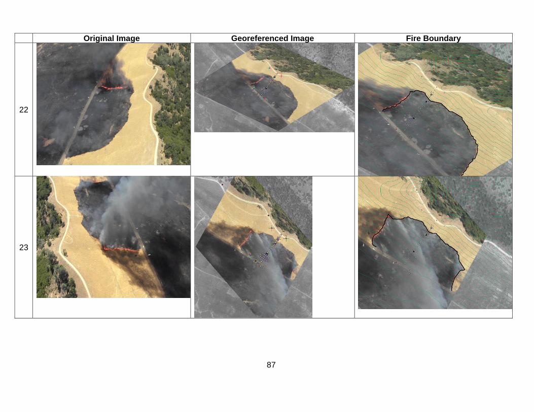
87

Original Image Georeferenced Image Fire Boundary

22

23

88

Original Image Georeferenced Image Fire Boundary

24

25

89

Appendix C - Georeference Points FHL Site 1

Photo Point #1/layer Point #2/layer Point #3/layer Point #4/layer Point #5/layer RMS Error

0 0_00_05_00

Ignition

FID50 LoNRefPost /

hl_field_instruments

FID48 LoSRefPost /

hl_field_instruments

FID2 Tower 1 / hl_field_instruments

- - 0.00

1 0_01_05_00 FID50 LoNRefPost

/ hl_field_instruments

FID48 LoSRefPost /

hl_field_instruments

FID2 Tower 1 / hl_field_instruments

- - 0.00

2 0_02_05_00 FID48 /

LoSRefPost hl_field_instruments

FID2 Tower 1 / hl_field_instruments

FID12 Tower 3 / hl_field_instruments

- - 0.00

3 0_03_05_00 FID50 LoNRefPost

/ hl_field_instruments

FID2 Tower1 / hl_field_instruments

FID5 Tower2 / hl_field_instruments

FID45 UpRAWS / hl_field_instruments

FID47 UpSRefPost /

hl_field_instruments

4.12393

4 0_04_05_00 FID50 LoNRefPost

/ hl_field_instruments

FID2 Tower1 / hl_field_instruments

FID5 Tower2 / hl_field_instruments

- - 0.00

5 6-

0_00_06_00

FID50 LoNRefPost /

hl_field_instruments

FID2 Tower1 / hl_field_instruments

FID5 Tower2 / hl_field_instruments

- - 0.00

6 6-

0_01_06_00

FID46 UpNRefPost /

hl_field_instruments

FID47 UpSRefPost /

hl_field_instruments

FID48 / LoSRefPost

hl_field_instruments - - 0.00

7 6-

0_02_06_00

FID46 UpNRefPost /

hl_field_instruments

FID47 UpSRefPost /

hl_field_instruments

FID48 / LoSRefPost

hl_field_instruments - - 0.00

8 6-

0_03_06_00

FID46 UpNRefPost /

hl_field_instruments

FID47 UpSRefPost /

hl_field_instruments

FID45 UpRAWS / hl_field_instruments

FID5 Tower2 / hl_field_instruments

FID1 Mustard / hl_veg_poly

5.22658

Photo Point #1/layer Point #2/layer Point #3/layer Point #4/layer Point #5/layer RMS Error

90

9 6-

0_04_06_00

FID46 UpNRefPost /

hl_field_instruments

FID45 UpRAWS / hl_field_instruments

FID5 Tower2 / hl_field_instruments

? - 2.945

63

10 6-

0_05_06_00

FID46 UpNRefPost /

hl_field_instruments

FID5 Tower2 / hl_field_instruments

FID49 LoCRefPost /

hl_field_instruments

FID1 Mustard / hl_veg_poly

- 6.813

17

11 6-

0_06_06_00

FID46 UpNRefPost /

hl_field_instruments

FID45 UpRAWS / hl_field_instruments

FID5 Tower2 / hl_field_instruments

FID1 Mustard / hl_veg_poly

? 5.647

31

12 7-

0_00_27_00

FID46 UpNRefPost /

hl_field_instruments

FID45 UpRAWS / hl_field_instruments

FID47 UpSRefPost /

hl_field_instruments

FID5 Tower2 / hl_field_instruments

FID48 / LoSRefPost

hl_field_instruments

3.91866

13 7-

0_01_27_00 FID45 UpRAWS / hl_field_instruments

FID2 Tower1 / hl_field_instruments

FID50 Camera / hl_field_instruments

FID48 / LoSRefPost

hl_field_instruments -

1.29630

14 7-

0_02_27_00

FID46 UpNRefPost /

hl_field_instruments

FID45 UpRAWS / hl_field_instruments

FID47 UpSRefPost /

hl_field_instruments

FID5 Tower2 / hl_field_instruments

FID48 / LoSRefPost

hl_field_instruments

3.19141

15 7-

0_03_27_00

FID46 UpNRefPost /

hl_field_instruments

FID45 UpRAWS / hl_field_instruments

FID5 Tower2 / hl_field_instruments

FID48 / LoSRefPost

hl_field_instruments

FID1 Mustard / hl_veg_poly

4.53064

16 8-

0_00_09_00

FID46 UpNRefPost /

hl_field_instruments

FID45 UpRAWS / hl_field_instruments

FID47 UpSRefPost /

hl_field_instruments

FID5 Tower2 / hl_field_instruments

FID49 LoCRefPost /

hl_field_instruments

FID1 Mustard / hl_veg_poly

4.82124

17 8-

0_01_09_00

FID46 UpNRefPost /

hl_field_instruments

FID45 UpRAWS / hl_field_instruments

FID47 UpSRefPost /

hl_field_instruments

FID12 Tower3 / hl_field_instruments

FID50 Camera / hl_field_instruments

FID49 LoCRefPost /

hl_field_instruments

10.30053

Photo Point #1/layer Point #2/layer Point #3/layer Point #4/layer Point #5/layer RMS Error

18 no image - - - - - -

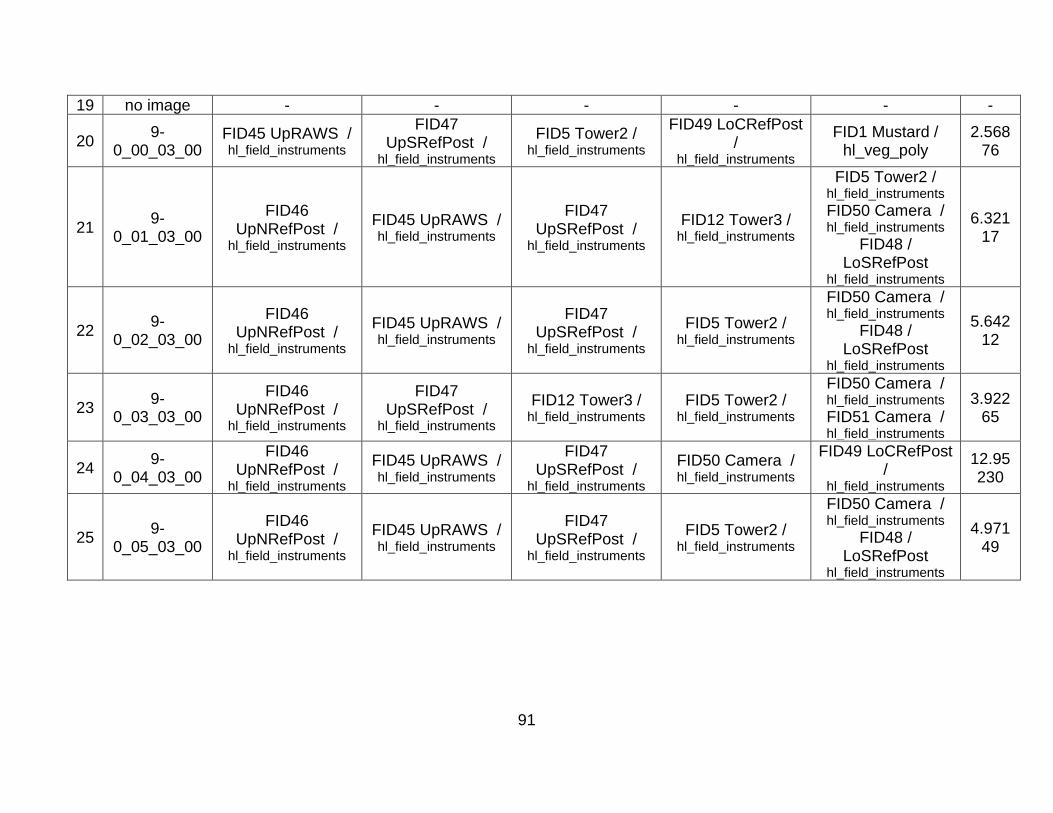
91

19 no image - - - - - -

20 9-

0_00_03_00 FID45 UpRAWS / hl_field_instruments

FID47 UpSRefPost /

hl_field_instruments

FID5 Tower2 / hl_field_instruments

FID49 LoCRefPost /

hl_field_instruments

FID1 Mustard / hl_veg_poly

2.56876

21 9-

0_01_03_00

FID46 UpNRefPost /

hl_field_instruments

FID45 UpRAWS / hl_field_instruments

FID47 UpSRefPost /

hl_field_instruments

FID12 Tower3 / hl_field_instruments

FID5 Tower2 / hl_field_instruments

FID50 Camera / hl_field_instruments

FID48 / LoSRefPost

hl_field_instruments

6.32117

22 9-

0_02_03_00

FID46 UpNRefPost /

hl_field_instruments

FID45 UpRAWS / hl_field_instruments

FID47 UpSRefPost /

hl_field_instruments

FID5 Tower2 / hl_field_instruments

FID50 Camera / hl_field_instruments

FID48 / LoSRefPost

hl_field_instruments

5.64212

23 9-

0_03_03_00

FID46 UpNRefPost /

hl_field_instruments

FID47 UpSRefPost /

hl_field_instruments

FID12 Tower3 / hl_field_instruments

FID5 Tower2 / hl_field_instruments

FID50 Camera / hl_field_instruments

FID51 Camera / hl_field_instruments

3.92265

24 9-

0_04_03_00

FID46 UpNRefPost /

hl_field_instruments

FID45 UpRAWS / hl_field_instruments

FID47 UpSRefPost /

hl_field_instruments

FID50 Camera / hl_field_instruments

FID49 LoCRefPost /

hl_field_instruments

12.95230

25 9-

0_05_03_00

FID46 UpNRefPost /

hl_field_instruments

FID45 UpRAWS / hl_field_instruments

FID47 UpSRefPost /

hl_field_instruments

FID5 Tower2 / hl_field_instruments

FID50 Camera / hl_field_instruments

FID48 / LoSRefPost

hl_field_instruments

4.97149