Observations and models of size distribution of KBOs

(summarize several articles)

Yeh, Lun-Wen

2006.12.26

References

1. Scott J. Kenyon & Jane X. Luu, 1998, AJ 115, 2136 Accretion in the earth Kuiper belt Ⅰ2. Scott J. Kenyon & Jane X. Luu, 1999, AJ 118, 1101 Accretion in the earth Kuiper belt Ⅱ3. Benz & Asphaug, 1999, Icarus 142, 5 Catastrophic disruption revisited4. Kenyon & Windhorst, 2001, AJ 547, L69 The Kuiper belt and Olbers’s paradox5. Scott J. Kenyon, 2002, PASP, 114, 265 Planet formation in the outer solar system6. Kenyon & Bromley, 2004, AJ 123, 1916 The size distribution of Kuiper belt objects7. http://cfa-www.harvard.edu/~kenyon/

Outline

• Overview• Observation constraints on size distribution

of KBOs• Numerical model• Analytic model • NEXT STEP…….

Outline

• Overview• Observation constraints on size distribution

of KBOs• Numerical model• Analytic model • NEXT STEP…….

• Overview

• 800-1000 observed KBOs with r ≥ 50 km• Heliocentric distance 35 AU-150AU• Inclination angle < 20º-30º

• The eccentricity 0.1-0.01.• The estimated numbers of KBO with r > 50 km is ~105;

the estimated total mass of Kuiper belt is ~ 0.1ME.

Overview

The cyan points indicate the positions of known KBOs as of January 2004.

The sharp decrease in the observed surface density at 10-30AU supports photoevaporation models where ionized hydrogen becomes unbound (Shu et al. 1993).

Adding H and He to achieve a solar abundance at 30-40 AU increases the mass in the Kuiper belt by a factor of ~ 30.

Material lost to orbital dynamics and to collisions in the belt may increase by another factor of 10-100.

Above two mechanisms let the initial mass of Kuiper belt within range of Σ~A-3/2.

The initial elemental abundances of the solar nebula were nearly identical to solar abundances. The surface density of the minimum -mass solar nebula follows from adding hydrogen and helium to each planet to reach a solar abundance.

Outline

• Overview• Observation constraints on size distribution

of KBOs• Numerical model• Analytic model • NEXT STEP…….

• Observation constraints on size distribution

of KBOs

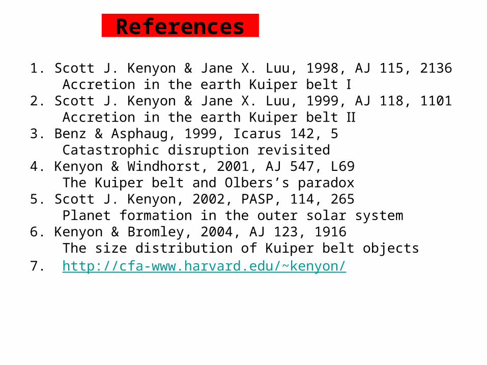
• In the planetesimal hypothesis, planetesimals with radii < 1-10km collide, merge, and grow into larger objects.

The accretion process yields a power-law size distribution with Nc ~ r -q , q~2.8-3.5 for 10-100 km and larger objects.

(Kenyon & Luu 1999b; Kenyon 2002)

• As the largest objects grow, their gravity stirs up the orbits of left over planetesimals to the disruption velocity. Collisions between leftover planetesimals then produce fragments instead of mergers.

For objects with radii of 1-10 km and smaller, this process yields a power-law size distribution with Nc ~ r -q , q~2.5.

(Stern 1996b; Stern & Colwell 1997a,1997b; Kenyon & Luu 1999a; Kenyon & Bromley 2004)

Observation constraints on size distribution of KBOs

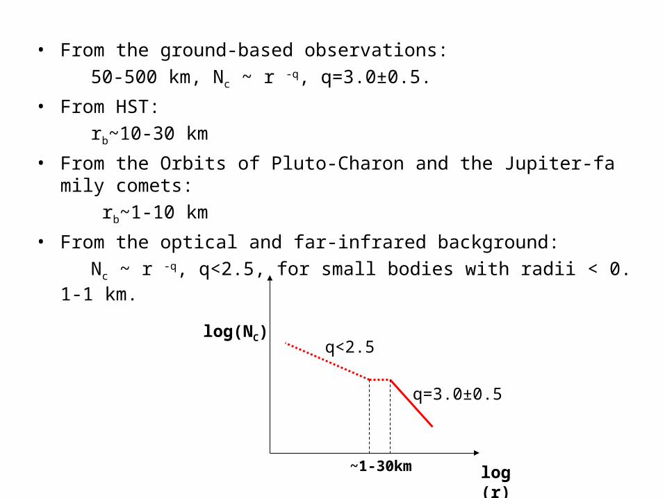
• From the ground-based observations:

50-500 km, Nc ~ r -q, q=3.0±0.5.

• From HST:

rb~10-30 km

• From the Orbits of Pluto-Charon and the Jupiter-family comets:

rb~1-10 km

• From the optical and far-infrared background:

Nc ~ r -q, q<2.5, for small bodies with radii < 0.1-1 km.

log(NC)

log(r)~1-30km

q=3.0±0.5

q<2.5

Outline

• Overview• Observation constraints on size distribution

of KBOs• Numerical model• Analytic model • NEXT STEP…….

• Numerical model

• Scott J. Kenyon and others developed a series of numerical model to simulate the evolution of KBOs.

Numerical model

1998 (Scott J. Kenyon & Jane X. Luu)

single annulus model: coagulation equation + velocity evolution.

1999 (Scott J. Kenyon & Jane X. Luu)

single annulus model: coagulation equation + velocity evolution + fragmentation.

2002 (Scott J. Kenyon)

multi annulus model: coagulation equation + velocity evolution + fragmentation.

2004 (Scott J. Kenyon & Benjamin C. Bromley)

multi annulus model : coagulation equation + N-body + velocity evolution + fragmentation.

The basic form of the coagulation equation:

Aij is the collision probability. nk, ni, nj are the numbers of planetesimal with mass of km0, im0, jm0 respectively.

1

2k

ij i j k ik ii j k i

dnA n n n A n

dt

• In the single annulus model (1999)• 32 AU-38 AU• M0=(1-100)ME , (Σ= Σ 0(A/1AU) -3/2 , Mmin~7-15ME)• The initial eccentricity and inclination: e=10-3-10-2, i=0.6e,• ρ=1.5 g/cm3.• S0=10-107 erg/g.• The initial size distribution take Nc ~ r0 –q , q=1.5,3.5,4.5; Nc=const*δ(r-r0); r0=1-80 m.

• To evolve the mass and velocity distributions in time, they solve the coagulation and energy conservation equations.

• The collisions, the gas drag, the viscous stirring, the dynamic friction and the fragmentation process.

• The lower limit to the formation timescale of KBOs is ~5-10 Myr.

The upper limit to the formation timescale of KBOs is ~100 Myr.

• The success KBO simulation criteria: r5 > 50 km Pluto formation, rmax > 1000 km

2.5

3.0

e0=10-3

S0=2*106 erg/g

e0=10-3

S0=2*106 erg/g

e0=10-3

S0=2*106 erg/g

r5

• The primary input parameters: M0, e0, S0, initial size distribution.

• The formation time is sensitive to M0 and e0, but is less sensitive to S0 and initial size distribution.

• NC ~ r -q, q ~ 2.5 for r < 0.1 km; q ~ 3.0 for r > 1-10 km. These slopes do not depend on M0, e0, S0 and initial size distri

bution.• Several Plutos and ~105 50 km radius KBOs form in MMSN wi

th e0~10-3 on timescales of 20-40Myr.• log rmax ~ 2.45 + 0.22logS0. Pluto formation needs S0 > 300 erg

/g.• After runaway growth, there are ~ 1%-2% of the initial mass in

50 km radius KBOs. The remaining mass is in 0.1-10 km radius KBOs. Fragmentation will gradually erode these smaller objects in to dust and remove them from Kuiper belt in timescales ~ 107 yr.

Outline

• Overview• Observation constraints on size distribution

of KBOs• Numerical model• Analytic model • NEXT STEP…….

• Analytic model

Analytic model

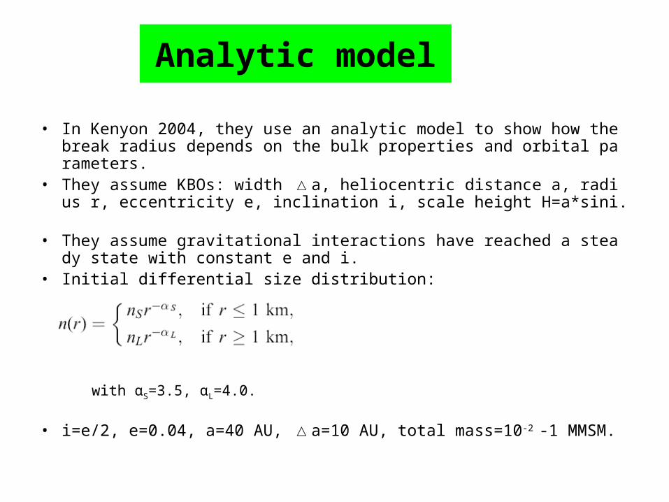
• In Kenyon 2004, they use an analytic model to show how the break radius depends on the bulk properties and orbital parameters.

• They assume KBOs: width a, heliocentric distance a, radius r, ec△centricity e, inclination i, scale height H=a*sini.

• They assume gravitational interactions have reached a steady state with constant e and i.

• Initial differential size distribution:

with αS=3.5, αL=4.0.

• i=e/2, e=0.04, a=40 AU, a=10 AU, total mass=10△ -2 -1 MMSM.

For a single KBO, the amount of mass accreted in collisions with all other KBOs during a time interval δt is

The amount of mass lost is

KBOs reach zero mass on a removal timescale

The collision rate for a KBO with radius r1 and all KBOs with radius r2 is

where V is the relative velocity, Ve is the escape velocity of a single body with mass m = m1 + m2.

The ejected mass mej is

The center-of-mass collision energy

The disruption energy

The energy need to remove 50% of the combined mass of two colliding objects

Benz & Asphaug 1999

Bulk component

gravity component

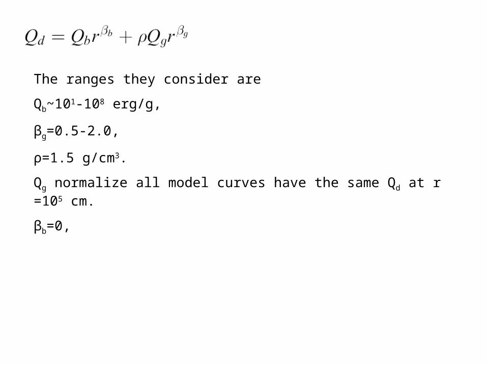
The ranges they consider are

Qb~101-108 erg/g,

βg=0.5-2.0,

ρ=1.5 g/cm3.

Qg normalize all model curves have the same Qd at r=105 cm.

βb=0,

The heavy dashed: 106 erg/g, 0.5

The heavy dot-dashed: 106 erg/g, 2.0

The light dashed: 103 erg/g, 0.5

The light dot-dashed: 103 erg/g, 2.0

The break radius is independent of the bulk strength Qb but is sensitive to βg.

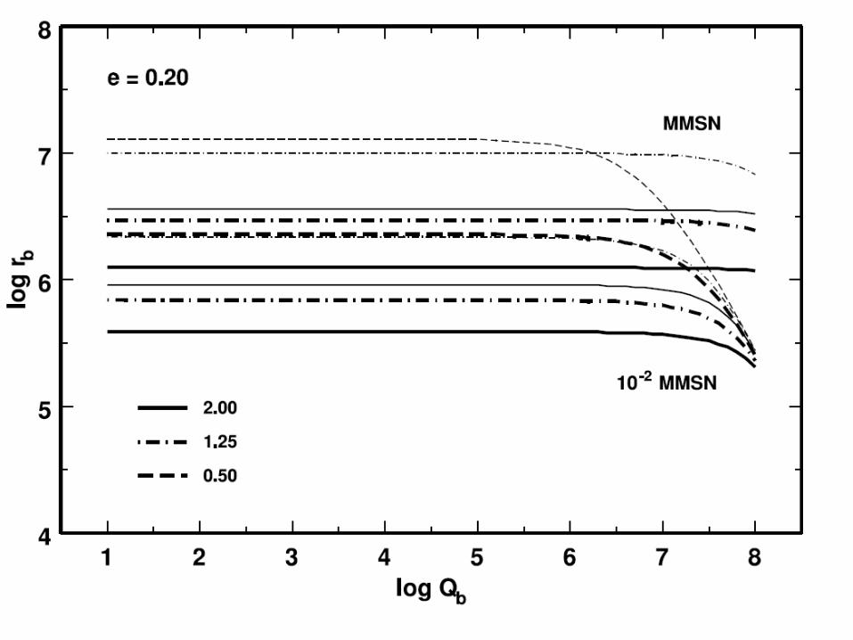
• The analytic model shows that a measured rb > 20 km requires a nebula with a mass in solids of at least 10% of the MMSN.

• The break in the sky surface density also favors a low bulk strength, Qb<106 erg/g

• The analytic model may also explain differences in the observed size distributions for different dynamical classes of KBOs.

Outline

• Overview• Observation constraints on size distribution

of KBOs• Numerical model• Analytic model • NEXT STEP…….• NEXT STEP…….

NEXT STEP…….

• Coagulation equation (Ohtsuki et al. 1990, Weterill 1990, Greenberg 1978).

Read some papers about N-body simulation.• Understand the basic picture of main-belt asteroids.

The differences of main-belt asteroids and KBOs. • The simulation for different classes of KBO maybe is one topic whic

h I can study.