Observations and Modeling of Tropical Planetary

Atmospheres

Thesis by

Anne Laraia

In Partial Fulfillment of the Requirements

for the Degree of

Doctor of Philosophy

California Institute of Technology

Pasadena, California

2016

(Defended June 22, 2015)

ii

c© 2016

Anne Laraia

All Rights Reserved

iii

To my brother Chris and my sister Emma:

Always together, never apart, maybe in distance but never at heart.

iv

Acknowledgments

I could not have completed this thesis without the support of my advisors, col-

leagues, friends and family. I had the great fortune of working with three faculty

members during my time at Caltech: Simona Bordoni, Andy Ingersoll and Tapio

Schneider. I’d like to thank Simona for taking me on as a third year student and

giving me guidance, independence and for being a role model. Andy Ingersoll encour-

aged and guided me in a project in planetary science even though it was out of my

discipline. Thank you to Tapio Schnedier for your continued support over the last 5

years. I’d also like to thank Paul Wennberg for your helpful feedback throughout my

PhD career and Andy Thompson for your willingness to join my committee on short

notice. I am deeply grateful for all of the opportunities, support and guidance with

which my committee has provided me during my time at Caltech.

Early on in my PhD experience I received a ton of help from older Caltech students,

post-docs and staff scientists. I’d like to thank Xavier Levine, Tim Merlis, and Yohai

Kaspi for helping me get started running the GCM. Special thanks to Junjun Liu

who provided a lot of guidance (and MATLAB code!) to me for my superrotation

project. Shawn Ewald got me started and answered continuous questions about IDL

for my Saturn project.

I have had the pleasure of sharing an office with some great students throughout

the years. I’d like to give a special thanks to Toby Bischoff, Jennifer Walker and

Jinqiang Chen for being great office mates who I’ve become close with over the years.

It has been a pleasure sitting next to you and getting to know you.

v

Thanks to Lindsay Yee, who started off as an older graduate student lending

advice and support and became a lifelong friend. I’d like to give another shout out

to Matt Coggon, who has been such a great friend to me. You have always been such

a reliable person that I can trust and whom I admire.

The Women Mentoring Women Program at Caltech was and is my safety net.

Through this program I was connected with my mentor, Jill Craven, who is my

Caltech sister. I treasure our friendship. Thank you so much for being there for

me for the past five years. I don’t think I could have done it without the constant

laughing together. You really brightened my life here.

None of this would have been possible without my loving and supportive fam-

ily. Thank you Mom and Dad for encouraging me and always being there for me.

Thanks to my brother Chris and my sister Emma for your visits, phone calls and love

throughout this five-year journey. I’m dedicating this to the two of you.

Lastly, I’d like to thank my incredible husband Steve Gardner, who embarked on

a long-distance relationship with me for 2.5 years when I decided to go to Caltech.

While I was a student at Caltech we got engaged, moved in together, and got married.

These five years will be special to me in so many ways, and you are a huge part of

that. Thank you for moving across the country to be with me, and for loving me and

supporting me through my ups and downs as a graduate student.

vi

Abstract

This thesis is a comprised of three different projects within the topic of tropical at-

mospheric dynamics. First, I analyze observations of thermal radiation from Saturn’s

atmosphere and from them, determine the latitudinal distribution of ammonia vapor

near the 1.5-bar pressure level. The most prominent feature of the observations is

the high brightness temperature of Saturn’s subtropical latitudes on either side of the

equator. After comparing the observations to a microwave radiative transfer model, I

find that these subtropical bands require very low ammonia relative humidity below

the ammonia cloud layer in order to achieve the high brightness temperatures ob-

served. We suggest that these bright subtropical bands represent dry zones created

by a meridionally overturning circulation.

Second, I use a dry atmospheric general circulation model to study equatorial su-

perrotation in terrestrial atmospheres. A wide range of atmospheres are simulated by

varying three parameters: the pole-equator radiative equilibrium temperature con-

trast, the convective lapse rate, and the planetary rotation rate. A scaling theory is

developed that establishes conditions under which superrotation occurs in terrestrial

atmospheres. The scaling arguments show that superrotation is favored when the

off-equatorial baroclinicity and planetary rotation rates are low. Similarly, superro-

tation is favored when the convective heating strengthens, which may account for the

superrotation seen in extreme global-warming simulations.

Third, I use a moist slab-ocean general circulation model to study the impact

of a zonally-symmetric continent on the distribution of monsoonal precipitation. I

vii

show that adding a hemispheric asymmetry in surface heat capacity is sufficient to

cause symmetry breaking in both the spatial and temporal distribution of precipita-

tion. This spatial symmetry breaking can be understood from a large-scale energetic

perspective, while the temporal symmetry breaking requires consideration of the dy-

namical response to the heat capacity asymmetry and the seasonal cycle of insolation.

Interestingly, the idealized monsoonal precipitation bears resemblance to precipita-

tion in the Indian monsoon sector, suggesting that this work may provide insight into

the causes of the temporally asymmetric distribution of precipitation over southeast

Asia.

viii

Contents

Acknowledgments iv

Abstract vi

1 Introduction 1

2 Analysis of Saturn’s thermal emission at 2.2-cm wavelength: spatial

distribution of ammonia vapor 6

3 Superrotation in terrestrial atmospheres 21

4 Symmetry breaking of precipitation patterns in a zonally symmetric

idealized monsoon 37

4.1 Introduction 37

4.2 Idealized GCM 41

4.2.1 GCM description 41

4.2.2 Simulations 42

4.3 Theory 44

4.4 GCM Results 47

4.5 Poleward boundary of ITCZ 50

4.5.1 Hemispheric energy imbalance 50

4.5.2 Quantitative estimates of the ITCZ position 54

4.6 Timing of Monsoon Onset/Retreat 56

ix

4.6.1 Caveats 56

4.6.2 Energy budget and ITCZ shifts 58

4.6.3 Surface temperature variations 64

4.6.4 Role of Dynamics 66

4.6.4.1 NH spring ITCZ transition 66

4.6.4.2 SH spring ITCZ transition 69

4.6.5 NH monsoon onset 71

4.7 Discussion 71

4.7.1 Relation to other theories 71

4.7.2 Comparison to observations and CMIP5 73

4.8 Conclusions 75

5 Conclusions 77

A Saturn’s thermal emission at 2.2-cm wavelength as imaged by the

Cassini RADAR radiometer 86

x

List of Figures

1.1 Absorbed shortwave, outgoing longwave, and net radiation (W m−2)

in Earth’s annual mean as a function of latitude. Net radiation is the

absorbed solar minus the emitted longwave radiation. Figure is from

Marshall and Plumb (2007). 2

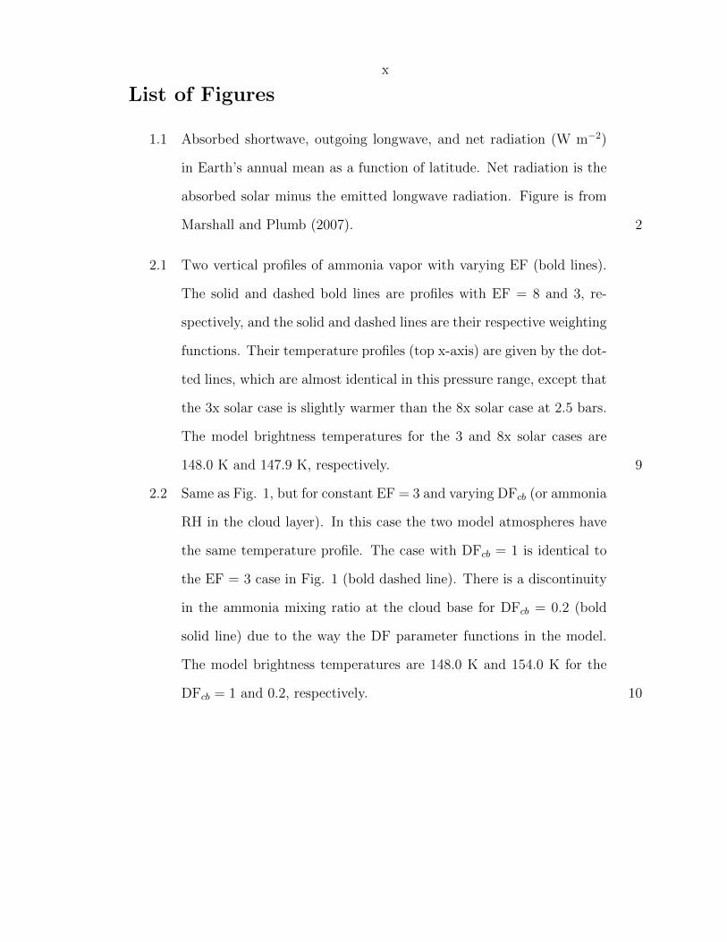
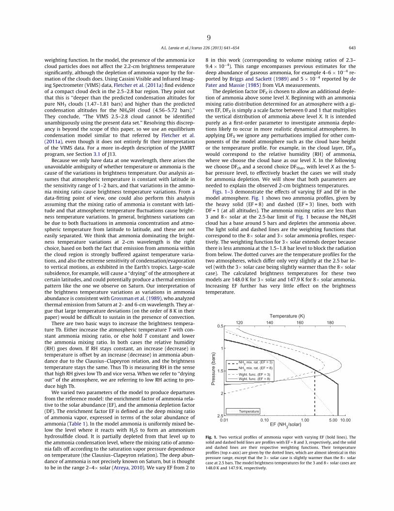
2.1 Two vertical profiles of ammonia vapor with varying EF (bold lines).

The solid and dashed bold lines are profiles with EF = 8 and 3, re-

spectively, and the solid and dashed lines are their respective weighting

functions. Their temperature profiles (top x-axis) are given by the dot-

ted lines, which are almost identical in this pressure range, except that

the 3x solar case is slightly warmer than the 8x solar case at 2.5 bars.

The model brightness temperatures for the 3 and 8x solar cases are

148.0 K and 147.9 K, respectively. 9

2.2 Same as Fig. 1, but for constant EF = 3 and varying DFcb (or ammonia

RH in the cloud layer). In this case the two model atmospheres have

the same temperature profile. The case with DFcb = 1 is identical to

the EF = 3 case in Fig. 1 (bold dashed line). There is a discontinuity

in the ammonia mixing ratio at the cloud base for DFcb = 0.2 (bold

solid line) due to the way the DF parameter functions in the model.

The model brightness temperatures are 148.0 K and 154.0 K for the

DFcb = 1 and 0.2, respectively. 10

xi

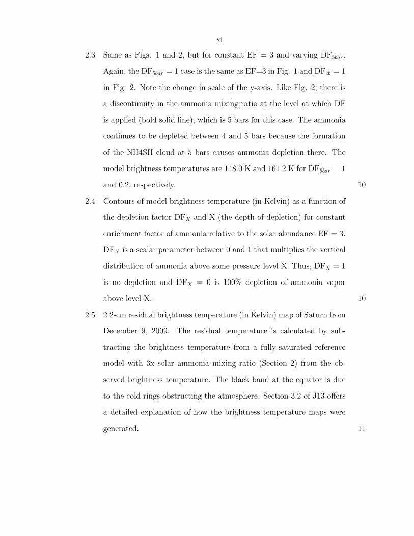
2.3 Same as Figs. 1 and 2, but for constant EF = 3 and varying DF5bar.

Again, the DF5bar = 1 case is the same as EF=3 in Fig. 1 and DFcb = 1

in Fig. 2. Note the change in scale of the y-axis. Like Fig. 2, there is

a discontinuity in the ammonia mixing ratio at the level at which DF

is applied (bold solid line), which is 5 bars for this case. The ammonia

continues to be depleted between 4 and 5 bars because the formation

of the NH4SH cloud at 5 bars causes ammonia depletion there. The

model brightness temperatures are 148.0 K and 161.2 K for DF5bar = 1

and 0.2, respectively. 10

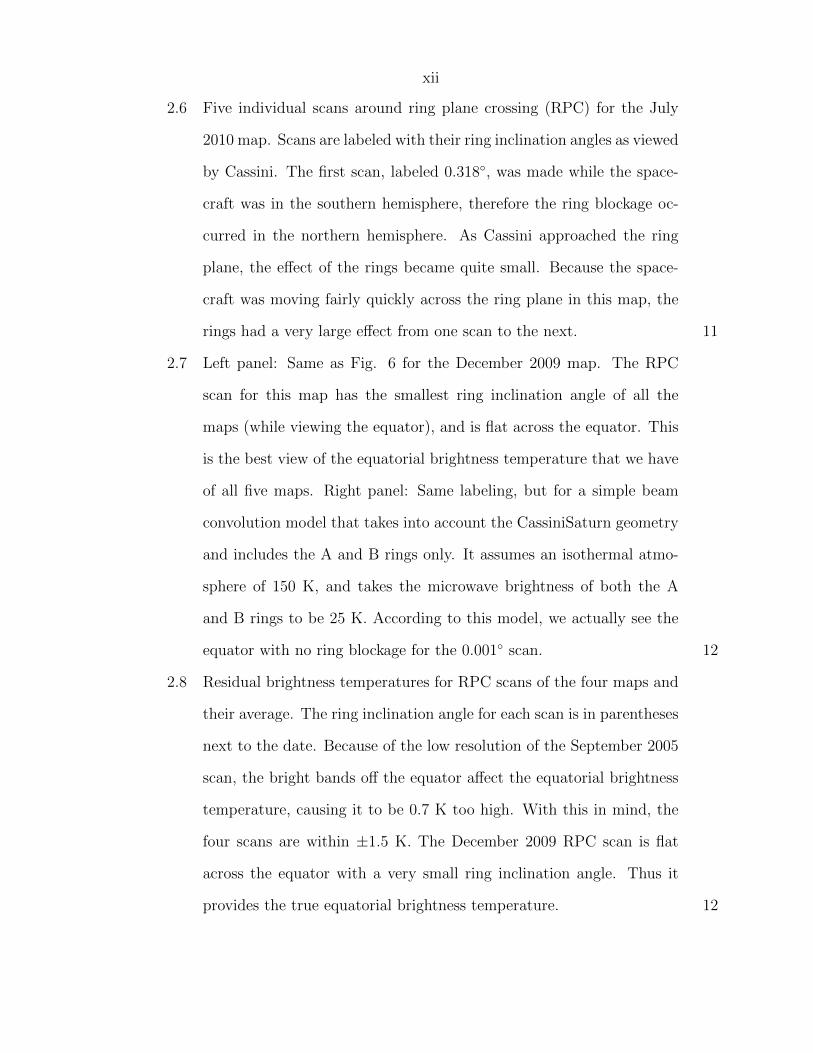
2.4 Contours of model brightness temperature (in Kelvin) as a function of

the depletion factor DFX and X (the depth of depletion) for constant

enrichment factor of ammonia relative to the solar abundance EF = 3.

DFX is a scalar parameter between 0 and 1 that multiplies the vertical

distribution of ammonia above some pressure level X. Thus, DFX = 1

is no depletion and DFX = 0 is 100% depletion of ammonia vapor

above level X. 10

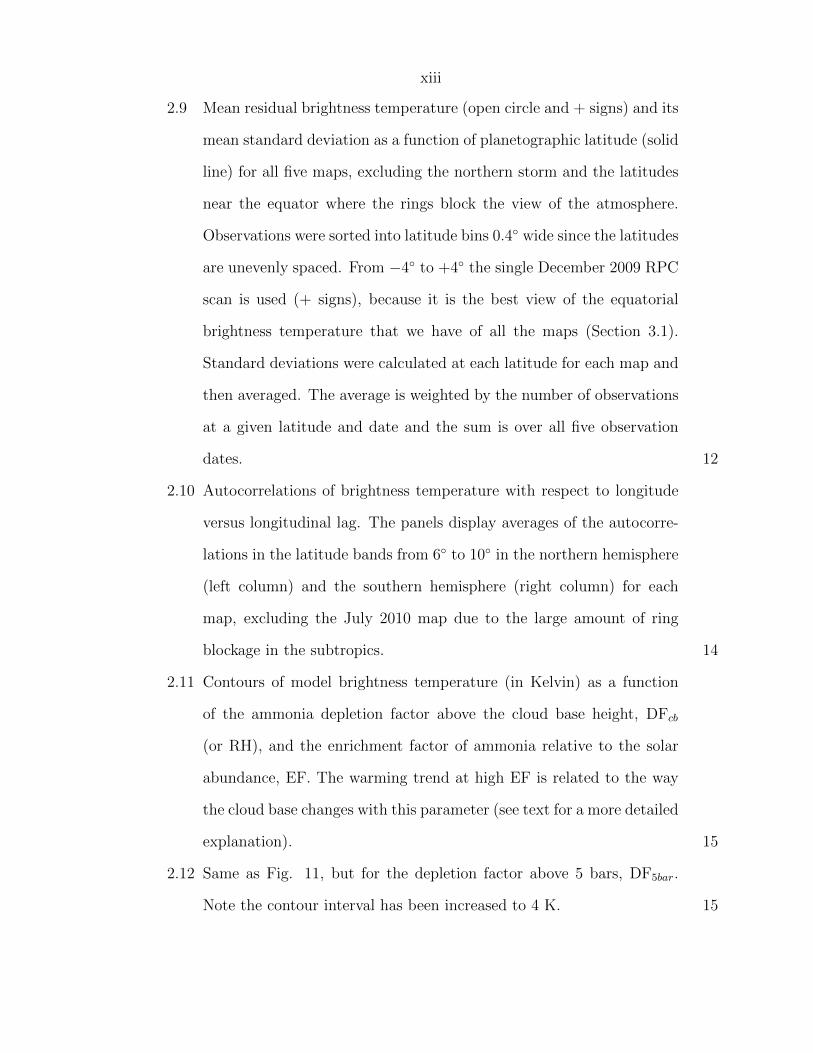
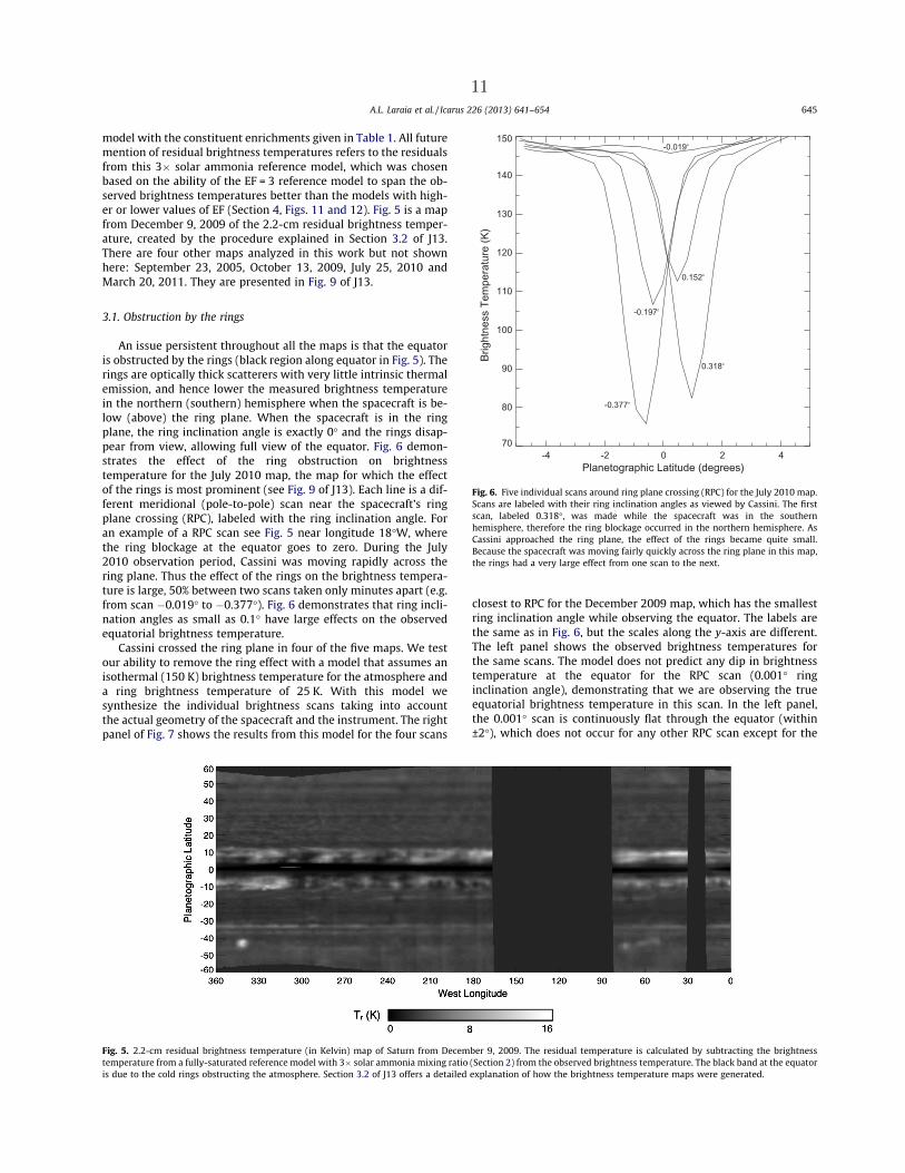
2.5 2.2-cm residual brightness temperature (in Kelvin) map of Saturn from

December 9, 2009. The residual temperature is calculated by sub-

tracting the brightness temperature from a fully-saturated reference

model with 3x solar ammonia mixing ratio (Section 2) from the ob-

served brightness temperature. The black band at the equator is due

to the cold rings obstructing the atmosphere. Section 3.2 of J13 offers

a detailed explanation of how the brightness temperature maps were

generated. 11

xii

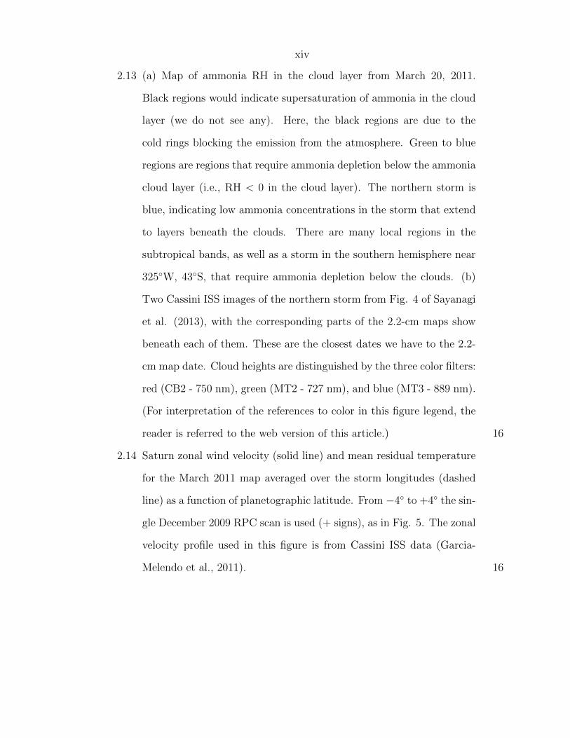
2.6 Five individual scans around ring plane crossing (RPC) for the July

2010 map. Scans are labeled with their ring inclination angles as viewed

by Cassini. The first scan, labeled 0.318, was made while the space-

craft was in the southern hemisphere, therefore the ring blockage oc-

curred in the northern hemisphere. As Cassini approached the ring

plane, the effect of the rings became quite small. Because the space-

craft was moving fairly quickly across the ring plane in this map, the

rings had a very large effect from one scan to the next. 11

2.7 Left panel: Same as Fig. 6 for the December 2009 map. The RPC

scan for this map has the smallest ring inclination angle of all the

maps (while viewing the equator), and is flat across the equator. This

is the best view of the equatorial brightness temperature that we have

of all five maps. Right panel: Same labeling, but for a simple beam

convolution model that takes into account the CassiniSaturn geometry

and includes the A and B rings only. It assumes an isothermal atmo-

sphere of 150 K, and takes the microwave brightness of both the A

and B rings to be 25 K. According to this model, we actually see the

equator with no ring blockage for the 0.001 scan. 12

2.8 Residual brightness temperatures for RPC scans of the four maps and

their average. The ring inclination angle for each scan is in parentheses

next to the date. Because of the low resolution of the September 2005

scan, the bright bands off the equator affect the equatorial brightness

temperature, causing it to be 0.7 K too high. With this in mind, the

four scans are within ±1.5 K. The December 2009 RPC scan is flat

across the equator with a very small ring inclination angle. Thus it

provides the true equatorial brightness temperature. 12

xiii

2.9 Mean residual brightness temperature (open circle and + signs) and its

mean standard deviation as a function of planetographic latitude (solid

line) for all five maps, excluding the northern storm and the latitudes

near the equator where the rings block the view of the atmosphere.

Observations were sorted into latitude bins 0.4 wide since the latitudes

are unevenly spaced. From −4 to +4 the single December 2009 RPC

scan is used (+ signs), because it is the best view of the equatorial

brightness temperature that we have of all the maps (Section 3.1).

Standard deviations were calculated at each latitude for each map and

then averaged. The average is weighted by the number of observations

at a given latitude and date and the sum is over all five observation

dates. 12

2.10 Autocorrelations of brightness temperature with respect to longitude

versus longitudinal lag. The panels display averages of the autocorre-

lations in the latitude bands from 6 to 10 in the northern hemisphere

(left column) and the southern hemisphere (right column) for each

map, excluding the July 2010 map due to the large amount of ring

blockage in the subtropics. 14

2.11 Contours of model brightness temperature (in Kelvin) as a function

of the ammonia depletion factor above the cloud base height, DFcb

(or RH), and the enrichment factor of ammonia relative to the solar

abundance, EF. The warming trend at high EF is related to the way

the cloud base changes with this parameter (see text for a more detailed

explanation). 15

2.12 Same as Fig. 11, but for the depletion factor above 5 bars, DF5bar.

Note the contour interval has been increased to 4 K. 15

xiv

2.13 (a) Map of ammonia RH in the cloud layer from March 20, 2011.

Black regions would indicate supersaturation of ammonia in the cloud

layer (we do not see any). Here, the black regions are due to the

cold rings blocking the emission from the atmosphere. Green to blue

regions are regions that require ammonia depletion below the ammonia

cloud layer (i.e., RH < 0 in the cloud layer). The northern storm is

blue, indicating low ammonia concentrations in the storm that extend

to layers beneath the clouds. There are many local regions in the

subtropical bands, as well as a storm in the southern hemisphere near

325W, 43S, that require ammonia depletion below the clouds. (b)

Two Cassini ISS images of the northern storm from Fig. 4 of Sayanagi

et al. (2013), with the corresponding parts of the 2.2-cm maps show

beneath each of them. These are the closest dates we have to the 2.2-

cm map date. Cloud heights are distinguished by the three color filters:

red (CB2 - 750 nm), green (MT2 - 727 nm), and blue (MT3 - 889 nm).

(For interpretation of the references to color in this figure legend, the

reader is referred to the web version of this article.) 16

2.14 Saturn zonal wind velocity (solid line) and mean residual temperature

for the March 2011 map averaged over the storm longitudes (dashed

line) as a function of planetographic latitude. From −4 to +4 the sin-

gle December 2009 RPC scan is used (+ signs), as in Fig. 5. The zonal

velocity profile used in this figure is from Cassini ISS data (Garcia-

Melendo et al., 2011). 16

xv

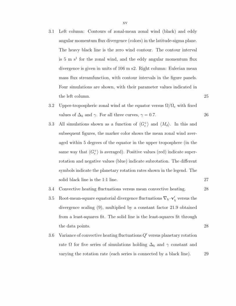
3.1 Left column: Contours of zonal-mean zonal wind (black) and eddy

angular momentum flux divergence (colors) in the latitude-sigma plane.

The heavy black line is the zero wind contour. The contour interval

is 5 m s1 for the zonal wind, and the eddy angular momentum flux

divergence is given in units of 106 m s2. Right column: Eulerian mean

mass flux streamfunction, with contour intervals in the figure panels.

Four simulations are shown, with their parameter values indicated in

the left column. 25

3.2 Upper-tropospheric zonal wind at the equator versus Ω/Ωe with fixed

values of ∆h and γ. For all three curves, γ = 0.7. 26

3.3 All simulations shown as a function of 〈G+e 〉 and 〈Md〉. In this and

subsequent figures, the marker color shows the mean zonal wind aver-

aged within 5 degrees of the equator in the upper troposphere (in the

same way that 〈G+e 〉 is averaged). Positive values (red) indicate super-

rotation and negative values (blue) indicate subrotation. The different

symbols indicate the planetary rotation rates shown in the legend. The

solid black line is the 1:1 line. 27

3.4 Convective heating fluctuations versus mean convective heating. 28

3.5 Root-mean-square equatorial divergence fluctuations ∇h ·v′χ versus the

divergence scaling (9), multiplied by a constant factor 21.9 obtained

from a least-squares fit. The solid line is the least-squares fit through

the data points. 28

3.6 Variance of convective heating fluctuationsQ′ versus planetary rotation

rate Ω for five series of simulations holding ∆h and γ constant and

varying the rotation rate (each series is connected by a black line). 29

xvi

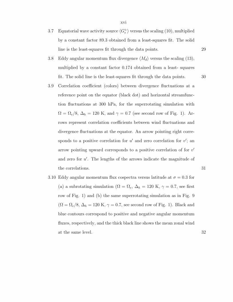
3.7 Equatorial wave activity source 〈G+e 〉 versus the scaling (10), multiplied

by a constant factor 89.3 obtained from a least-squares fit. The solid

line is the least-squares fit through the data points. 29

3.8 Eddy angular momentum flux divergence 〈Md〉 versus the scaling (13),

multiplied by a constant factor 0.174 obtained from a least- squares

fit. The solid line is the least-squares fit through the data points. 30

3.9 Correlation coefficient (colors) between divergence fluctuations at a

reference point on the equator (black dot) and horizontal streamfunc-

tion fluctuations at 300 hPa, for the superrotating simulation with

Ω = Ωe/8, ∆h = 120 K, and γ = 0.7 (see second row of Fig. 1). Ar-

rows represent correlation coefficients between wind fluctuations and

divergence fluctuations at the equator. An arrow pointing right corre-

sponds to a positive correlation for u′ and zero correlation for v′; an

arrow pointing upward corresponds to a positive correlation of for v′

and zero for u′. The lengths of the arrows indicate the magnitude of

the correlations. 31

3.10 Eddy angular momentum flux cospectra versus latitude at σ = 0.3 for

(a) a subrotating simulation (Ω = Ωe, ∆h = 120 K, γ = 0.7, see first

row of Fig. 1) and (b) the same superrotating simulation as in Fig. 9

(Ω = Ωe/8, ∆h = 120 K, γ = 0.7, see second row of Fig. 1). Black and

blue contours correspond to positive and negative angular momentum

fluxes, respectively, and the thick black line shows the mean zonal wind

at the same level. 32

xvii

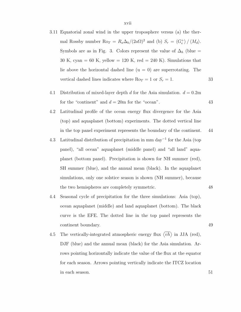
3.11 Equatorial zonal wind in the upper troposphere versus (a) the ther-

mal Rossby number RoT = Ra∆h/(2aΩ)2 and (b) Sr = 〈G+e 〉 / 〈Md〉.

Symbols are as in Fig. 3. Colors represent the value of ∆h (blue =

30 K, cyan = 60 K, yellow = 120 K, red = 240 K). Simulations that

lie above the horizontal dashed line (u = 0) are superrotating. The

vertical dashed lines indicates where RoT = 1 or Sr = 1. 33

4.1 Distribution of mixed-layer depth d for the Asia simulation. d = 0.2m

for the “continent” and d = 20m for the “ocean”. 43

4.2 Latitudinal profile of the ocean energy flux divergence for the Asia

(top) and aquaplanet (bottom) experiments. The dotted vertical line

in the top panel experiment represents the boundary of the continent. 44

4.3 Latitudinal distribution of precipitation in mm day−1 for the Asia (top

panel), “all ocean” aquaplanet (middle panel) and “all land” aqua-

planet (bottom panel). Precipitation is shown for NH summer (red),

SH summer (blue), and the annual mean (black). In the aquaplanet

simulations, only one solstice season is shown (NH summer), because

the two hemispheres are completely symmetric. 48

4.4 Seasonal cycle of precipitation for the three simulations: Asia (top),

ocean aquaplanet (middle) and land aquaplanet (bottom). The black

curve is the EFE. The dotted line in the top panel represents the

continent boundary. 49

4.5 The vertically-integrated atmospheric energy flux⟨vh

⟩in JJA (red),

DJF (blue) and the annual mean (black) for the Asia simulation. Ar-

rows pointing horizontally indicate the value of the flux at the equator

for each season. Arrows pointing vertically indicate the ITCZ location

in each season. 51

xviii

4.6 ∆(S − L) = (S − L)NH − (S − L)SH is the hemispheric asymmetry in

TOA radiation as a function of latitude, shown for JJA (red), DJF

(blue), and the annual mean (black). Negative values indicate that the

NH receives less TOA radiation than the SH, and vice-versa. 52

4.7 Average distribution of F net = S−L−O−Os−A with latitude in JJA

(red), DJF (blue) and the annual mean (black) for the Asia simulation. 53

4.8 Seasonal cycle of the atmospheric energy flux at the equator (left)

and its divergence (right). Three simulations are shown: The Asia

simulation (top row), the 20-m aquaplanet (middle row) and the 0.2-m

aquaplanet (bottom row). The two terms plotted are the numerator

and denominator of δ in Eq. (4.4), respectively. Shading represents the

transition time, during which the EFE crosses the equator. Blue arrows

indicate monsoon onset, as defined by the development of a deep, cross-

equatorial circulation. The red arrows in the top panel indicate the

beginning of the brief double-ITCZ period during NH spring for the

Asia simulation. 59

4.9 Seasonal cycle of the terms comprising the net energy input to the

equatorial atmosphere. (top) S0 −O0 and L0 for the Asia simulation,

(middle) S0 −O0 − L0 and the ocean energy storage Os0 for the Asia

simulation, and (bottom) equatorial surface temperature for all three

simulations. Shading and arrows are the same as in Figure 4.8. 62

4.10 Seasonal cycle of the surface latent heat flux LH, surface wind speed

U , and vertical moisture gradient (qs − q) at the equator for the all

ocean aquaplanet (top) and the Asia simulation (bottom). Shading

and arrows are the same as in Figure 4.8. All terms are normalized by

their maximum value at the equator. 64

xix

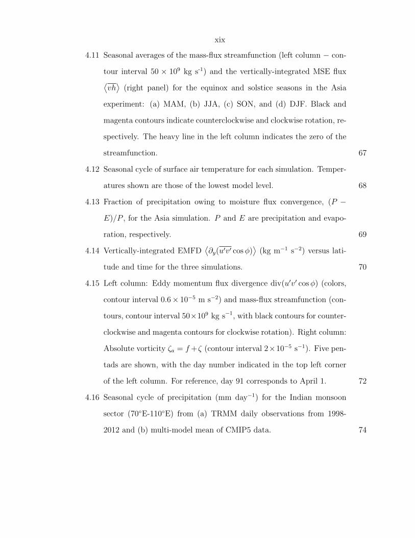
4.11 Seasonal averages of the mass-flux streamfunction (left column − con-

tour interval 50 × 109 kg s-1) and the vertically-integrated MSE flux⟨vh

⟩(right panel) for the equinox and solstice seasons in the Asia

experiment: (a) MAM, (b) JJA, (c) SON, and (d) DJF. Black and

magenta contours indicate counterclockwise and clockwise rotation, re-

spectively. The heavy line in the left column indicates the zero of the

streamfunction. 67

4.12 Seasonal cycle of surface air temperature for each simulation. Temper-

atures shown are those of the lowest model level. 68

4.13 Fraction of precipitation owing to moisture flux convergence, (P −

E)/P , for the Asia simulation. P and E are precipitation and evapo-

ration, respectively. 69

4.14 Vertically-integrated EMFD⟨∂y(u′v′ cosφ)

⟩(kg m−1 s−2) versus lati-

tude and time for the three simulations. 70

4.15 Left column: Eddy momentum flux divergence div(u′v′ cosφ) (colors,

contour interval 0.6× 10−5 m s−2) and mass-flux streamfunction (con-

tours, contour interval 50×109 kg s−1, with black contours for counter-

clockwise and magenta contours for clockwise rotation). Right column:

Absolute vorticity ζa = f+ζ (contour interval 2×10−5 s−1). Five pen-

tads are shown, with the day number indicated in the top left corner

of the left column. For reference, day 91 corresponds to April 1. 72

4.16 Seasonal cycle of precipitation (mm day−1) for the Indian monsoon

sector (70E-110E) from (a) TRMM daily observations from 1998-

2012 and (b) multi-model mean of CMIP5 data. 74

xx

A.1 Scan pattern of the radiometer for a mapping campaign in 2009, in

inertial space and time (upper panel), and as tracks on the surface of

Saturn (lower panel). The underlying map is derived from the data

as described later in this paper. The 0.36 half-power beamwidth

(HPBW) is shown in the upper panel for reference. 89

A.2 Beam footprints on Saturn at two extremes of resolution. Shown are

the half-power beam footprints on two partial maps of Saturn from

September 2005. 90

A.3 Microwave absorption profiles at 2-cm wavelength for possible absorb-

ing constituents through the NH3 cloud region. The atmospheric com-

position is that of our reference model as given in Table 4. The dotted

lines indicate conservative estimates for various particulate absorbers

as indicated, while the other lines represent individual gases identi-

fied in the legend. The curve labeled CIA includes the sum of H2-H2,

H2-He, and H2-CH4 collision-induced absorption. 91

A.4 Atmospheric model used to compute reference brightness tempera-

tures. The temperature (dotted line) and NH3 mixing ratio in units

of solar abundance (thick solid line) are shown as a function of pres-

sure and altitude in the vicinity of the ammonia cloud region in the

atmosphere. The reference model assumes 100% relative humidity for

ammonia above its saturation level, while the light solid line shows

a case for 50% relative humidity. The decrease in NH3 mixing ratio

above the 5-bar level is due to reaction with H2S to form NH4SH ice.

The dashed line shows the 2.2-cm wavelength weighting function in

arbitrary linear units at normal incidence for the reference model. 92

xxi

A.5 Initial steps in the calibration process are illustrated for the December

2009 map. Each 1-s measurement from this observing campaign is

plotted as a single point in all panels. Top to bottom, the panels show

respectively: (a) the time-ordered data with an initial scale calibration

but without a baseline correction; (b) model convolutions over the

reference model to obtain estimates of the sidelobe contributions; (c) a

derived zero offset correction; and (d) the final calibrated and baseline-

adjusted antenna temperatures. The right-hand section of each panel

shows a subset of the data on an expanded time scale centered near

the center of the pass. 93

A.6 Global map of brightness temperature residuals from December 2009,

before further adjustment to remove artifacts. 94

A.7 Mean values by scan of “quiescent” latitudinal bands in northern and

southern hemispheres, plotted by elapsed time and compared with

range for each map. Each point (+) shows the mean brightness tem-

peratures of each individual scan in these bands, plotted relative to

the overall mean, with values given on the left-hand scale. The solid

curves show range in units of Saturn radii as given on the right-hand

scale. 95

A.8 Values of global mean quiescent band brightness temperatures as de-

scribed in the text for each calibrated Saturn map relative to that for

September 2005. The dashed line is a linear fit that we take to indicate

a radiometer gain drift with time. 95

xxii

A.9 Final cylindrical maps of Saturn from the five observation campaigns.

The absolutely calibrated maps are shown in the five panels as resid-

uals from a model that assumes ammonia to be fully saturated in the

cloud-forming region. The dashed and dotted lines indicate periapsis

and ring plane crossings, respectively (there were no observations made

exactly at ring plane crossing for the 2005 and 2011 maps). Planeto-

graphic latitudes are indicated by black ticks on the vertical scales,

planetocentric by white. The unobserved portions of the maps are

shaded to the equivalent brightness for the fully saturated model, so

that, except for the ring blockage around the equator, the maps indi-

cate that the ammonia cloud region is everywhere unsaturated. Orbital

characteristics and mapping details are given in Tables 2 and 3, and

uncertainties and caveats concerning the maps are given in the text. 96

A.10 Brightness distribution through the region of ring blockage. The cali-

brated brightness temperature is shown for one scan in latitude around

the time of peak ring inclination with respect to the spacecraft in the

July 2010 mapping campaign. The boundaries between the rings are

indicated. The Cassini Division is clearly seen. 97

A.11 Differenced longitudinal averages of the latitudinal brightness distri-

bution for the three maps in which the spacecraft Y-axis was inverted

partway through the observation. The longitudinal brightness at each

0.5 in latitude was averaged separately for the two orientations and

subtracted to search for an asymmetry in the NS sidelobe pattern.

None is apparent. 97

xxiii

A.12 The great northern storm of 2010. The section of the March 2011

map containing the storm is shown in the upper panel with a stretch

that enhances the high brightness regions. The lower panel gives the

half-power footprints (showing only every fourth footprint in latitude). 98

A.13 Longitudinal averages of the latitudinal brightness distribution for all

maps. The equatorial region within 5 is generally dominated by ring

blockage, as is the region from -20 to 0 for the July 2010 map -

the plunge to negative residuals in these regions is an artifact of this.

The dotted lines indicate model brightness residuals that would be

observed if cloud relative humidity were allowed to vary relative to the

fully saturated model. 98

xxiv

List of Tables

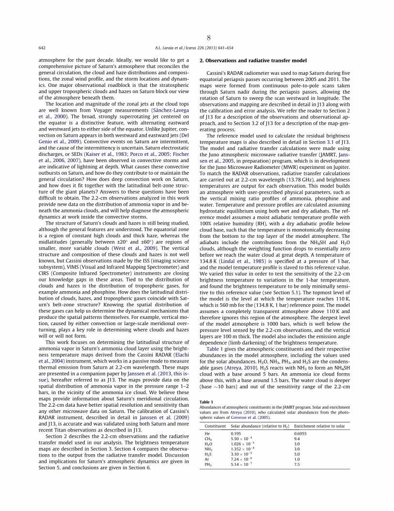
2.1 Abundances of atmospheric constituents in the JAMRT program. Solar

and enrichment values are from Atreya (2010), who calculated solar

abundances from the photospheric values of Grevesse et al. (2005). 8

3.1 Parameters varied in the 60 simulations: Planetary rotation rate Ω (as a

multiple of Earth’s rotation rate Ωe), pole-equator temperature contrast

in radiative equilibrium ∆h, and rescaling parameter γ of the convective

lapse rate Γ = γΓd. 24

A.1 Nominal radiometer characteristics. 88

A.2 Mapping orbit characteristics. 88

A.3 Mapping details. 89

A.4 Composition of the Saturn reference model atmosphere (based on Atreya

(2010)). 91

1

Chapter 1

Introduction

Earth’s tropical atmosphere, residing in the region surrounding the equator, has

very different dynamical characteristics than those of other latitudes and is signifi-

cantly less well understood. In the tropics, horizontal atmospheric temperature and

pressure gradients are constrained to be small outside of the boundary layer, and

the effects of planetary rotation are smallest at the equator where the Coriolis force

goes to zero. Thus, quasi-geostrophy that governs middle and high latitude dynamics

is not appropriate for the tropics. Also, unlike middle and high latitudes, diabatic

heating plays a large role in the energy budget in the tropics.

Earth’s tropics is characterized by an annually-averaged excess of net radiation:

more incoming solar radiation is absorbed than outgoing longwave radiation emitted

(Fig. 1.1). The extratropics, on the other hand, have a deficit of net radiation. This

occurs because spherical planetary bodies with Earth-like obliquities are differentially

heated by the sun such that, over the course of a year, the equator receives more sun-

light than the poles. To balance this excess radiation in the tropics and deficit at

higher latitudes, the atmosphere and ocean must transport energy from the equator

toward the poles. On Earth, the poleward energy transport of the atmosphere is ac-

complished by the meridionally overturning circulation in the tropics and by weather

systems, or eddies, in midlatitudes.

In 1735, Hadley provided the first comprehensive theory of the tropical overturn-

2

Figure 1.1: Absorbed shortwave, outgoing longwave, and net radiation (W m−2) inEarth’s annual mean as a function of latitude. Net radiation is the absorbed solarminus the emitted longwave radiation. Figure is from Marshall and Plumb (2007).

ing circulation, with solar heating in the tropics causing the air to rise, flow poleward

at upper levels, and sink by differential cooling at higher latitudes. The return flow

occurs at the surface, where the effects of friction balance the Coriolis force, causing

the surface winds to be deflected to the west. He postulated that angular momentum

conservation in the upper branch of the circulation causes zonal winds to become

more westerly as the air moves poleward, and that when the air sinks the wester-

lies are transferred to the surface. Drag on the surface easterlies transfers angular

momentum from the surface to the atmosphere in low latitudes, and drag on the

westerlies in higher latitudes transfers it back to the surface. Thus Earth’s angular

momentum is conserved. This thermally direct circulation therefore transports both

heat and angular momentum from the tropics to higher latitudes. Since then the

importance of large-scale eddies in maintaining angular-momentum conservation has

been demonstrated. These eddies make up much of the atmospheric transport of heat

and momentum in midlatitudes.

However, Hadley wasn’t too far off: A meridional cross-section of Earth’s tropical

atmosphere in the annual mean reveals two overturning cells, known as Hadley cells,

that transport heat and momentum from the equator toward the poles. In the zonal

3

direction, there are weak easterlies at all levels extending from 30N to 30S, accom-

panied by weak meridional temperature gradients. The ascending branch of Hadley

cell, located at the boundary of the two cells, is the intertropical convergence zone

(ITCZ). The ITCZ is a band of deep convection (e.g., thunderstorms) that moves

north and south in the tropics with the seasons. Monsoons are a manifestation of

the seasonal migrations of the ITCZ over subtropical continents, whereby an onset

of intense rainfall occurs that persists through the summer months. Most of the

annually-averaged rainfall on Earth falls in tropical latitudes, which makes under-

standing tropical atmospheric dynamics and how it changes with climate a priority.

Although there is pressing motivation to understand tropical dynamics on our own

planet, tropical atmospheric dynamics is an interesting fluid dynamical problem in

general. The different sizes, surfaces, rotation rates, orbital parameters, and chemical

makeups of the planets contribute to the wide range of atmospheres present in our so-

lar system. Venus, Jupiter and Saturn, for example, have superrotating atmospheres,

meaning that the atmosphere is spinning faster than the solid-body planet (or the

core of the planet) itself at the equator. This is in stark contrast to Earth, which has

a subrotating atmosphere, and suggests that superrotation may be the norm rather

than the exception.

This thesis explores three elements of tropical planetary atmospheres. First, I use

microwave observations of Saturn’s atmosphere to determine the gaseous ammonia

distribution and hypothesize about what it implies for the tropical circulation (Chap-

ter 2). Unlike on Earth, observations of Saturn’s thick atmosphere, especially below

the main cloud deck, are scarce and difficult to make. In this chapter I determined

the latitudinal distribution of ammonia, a condensable vapor in Saturn’s atmosphere,

near the 1-bar level. Because ammonia is condensable, it is analogous to water vapor

in Earth’s atmosphere. When the atmosphere is saturated or very dry (e.g., 100%

versus 0% relative humidity), one might be able to infer the direction of vertical mo-

4

tion in the atmosphere. On Earth, for example, there are dry regions in the subtropics

on either side of the equator. This is where Earth’s deserts are located. These dry

regions coincide with atmospheric downwelling from the Hadley circulation. We view

ammonia vapor similarly on Saturn, and speculate on the tropical circulation given

the latitudinal distribution of ammonia vapor.

In Chapter 3 I use an atmospheric general circulation model (GCM) to study

superrotation in terrestrial atmospheres (i.e., planets with solid surfaces). Superro-

tation occurs when the angular momentum of the atmosphere exceeds that of the

solid-body planet beneath it, or, in the case of the gas giants, relative to the rotation

of their cores and magnetic fields. Superrotation is ubiquitous in our solar system,

but, as previously mentioned, it is not a phenomenon observed in Earth’s troposphere.

Earth-like climate models have, however, demonstrated a transition to superrotation

under extreme global warming scenarios (e.g., Caballero and Huber 2010). The work

done in Chapter 3 helps us to understand under which conditions superrotation arises

in terrestrial atmospheres.

Finally, I use a slab ocean idealized GCM to study the fundamental dynamics of

a monsoon system over an idealized continent (Chapter 4). Monsoons are seasonal

migrations of the intertropical convergence zone, or ITCZ, over subtropical continents.

Although monsoons are important features of the summertime tropical circulation on

Earth, we still lack a coherent understanding of them. In this work we find that

the seasonal progression of the ITCZ, even over a very gross idealization of an Asia

continental configuration and in a model with simplified physics, mimics that of the

ITCZ in the Indian monsoon sector. Idealized studies like the one in Chapter 4

may provide insights into fundamental dynamical and thermodynamical mechanisms

controlling the existence and seasonality of monsoons and provide useful constraints

for diagnosing output from comprehensive GCMs, such as those in the CMIP5 archive.

Although the three projects presented in this thesis use different methods and

5

have different specific motivations, the underlying theme is clear: We want to have

a comprehensive understanding of tropical atmospheric dynamics. Both models and

observations are essential to this, and I have used both here. Different planets present

different challenges and push the limits of our understanding. The contributions of

this work bring us closer to achieving this goal.

6

Chapter 2

Analysis of Saturn’s thermalemission at 2.2-cm wavelength:spatial distribution of ammoniavapor

0Reprinted from Elsevier. Formal publication located at doi:10.1016/j.icarus.2013.06.017

Analysis of Saturn’s thermal emission at 2.2-cm wavelength: Spatialdistribution of ammonia vapor

A.L. Laraia a,⇑, A.P. Ingersoll a, M.A. Janssen b, S. Gulkis b, F. Oyafuso b, M. Allison c

a California Institute of Technology, Pasadena, CA 91125, United Statesb Jet Propulsion Laboratory, California Institute of Technology, Pasadena, CA 91109, United Statesc NASA Goddard Institute for Space Studies, New York, NY 10025, United States

a r t i c l e i n f o

Article history:Available online 27 June 2013

Keywords:Saturn, AtmosphereAtmospheres, StructureAtmospheres, CompositionAtmospheres, DynamicsRadio observations

a b s t r a c t

This work focuses on determining the latitudinal structure of ammonia vapor in Saturn’s cloud layer near1.5 bars using the brightness temperature maps derived from the Cassini RADAR (Elachi et al. [2004],Space Sci. Rev. 115, 71–110) instrument, which works in a passive mode to measure thermal emissionfrom Saturn at 2.2-cm wavelength. We perform an analysis of five brightness temperature maps thatspan epochs from 2005 to 2011, which are presented in a companion paper by Janssen et al. (Janssen,M.A., Ingersoll, A.P., Allison, M.D., Gulkis, S., Laraia, A.L., Baines, K., Edgington, S., Anderson, Y., Kelleher,K., Oyafuso, F. [2013]. Icarus, this issue). The brightness temperature maps are representative of the spa-tial distribution of ammonia vapor, since ammonia gas is the only effective opacity source in Saturn’satmosphere at 2.2-cm wavelength. Relatively high brightness temperatures indicate relatively lowammonia relative humidity (RH), and vice versa. We compare the observed brightness temperatures tobrightness temperatures computed using the Juno atmospheric microwave radiative transfer (JAMRT)program which includes both the means to calculate a tropospheric atmosphere model for Saturn andthe means to carry out radiative transfer calculations at microwave frequencies. The reference atmo-sphere to which we compare has a 3 solar deep mixing ratio of ammonia (we use 1.352 104 forthe solar mixing ratio of ammonia vapor relative to H2; see Atreya [2010]. In: Galileo’s Medicean Moons– Their Impact on 400 years of Discovery. Cambridge University Press, pp. 130–140 (Chapter 16)) and isfully saturated above its cloud base. The maps are comprised of residual brightness temperatures—observed brightness temperature minus the model brightness temperature of the saturated atmosphere.

The most prominent feature throughout all five maps is the high brightness temperature of Saturn’ssubtropical latitudes near ±9 (planetographic). These latitudes bracket the equator, which has some ofthe lowest brightness temperatures observed on the planet. The observed high brightness temperaturesindicate that the atmosphere is sub-saturated, locally, with respect to fully saturated ammonia in thecloud region. Saturn’s northern hemisphere storm was also captured in the March 20, 2011 map, andis very bright, reaching brightness temperatures of 166 K compared to 148 K for the saturated atmo-sphere model. We find that both the subtropical bands and the 2010–2011 northern storm require verylow ammonia RH below the ammonia cloud layer, which is located near 1.5 bars in the reference atmo-sphere, in order to achieve the high brightness temperatures observed. The disturbances in the southernhemisphere between 42 and 47 also require very low ammonia RH at levels below the ammoniacloud base. Aside from these local and regional anomalies, we find that Saturn’s atmosphere has on aver-age 70 ± 15% ammonia relative humidity in the cloud region. We present three options to explain the high2.2-cm brightness temperatures. One is that the dryness, i.e., the low RH, is due to higher than averageatmospheric temperatures with constant ammonia mixing ratios. The second is that the bright subtrop-ical bands represent dry zones created by a meridionally overturning circulation, much like the Hadleycirculation on Earth. The last is that the drying in both the southern hemisphere storms and 2010–2011 northern storm is an intrinsic property of convection in giant planet atmospheres. Some combina-tion of the latter two options is argued as the likely explanation.

2013 Elsevier Inc. All rights reserved.

1. Introduction

The instruments on board the Cassini orbiter have provided thegiant planets community with a plethora of data on Saturn’s

0019-1035/$ - see front matter 2013 Elsevier Inc. All rights reserved.http://dx.doi.org/10.1016/j.icarus.2013.06.017

⇑ Corresponding author.E-mail address: alaraia@caltech.edu (A.L. Laraia).

Icarus 226 (2013) 641–654

Contents lists available at SciVerse ScienceDirect

Icarus

journal homepage: www.elsevier .com/locate / icarus

7

atmosphere for the past decade. Ideally, we would like to get acomprehensive picture of Saturn’s atmosphere that reconciles thegeneral circulation, the cloud and haze distributions and composi-tions, the zonal wind profile, and the storm locations and dynam-ics. One major observational roadblock is that the stratosphericand upper tropospheric clouds and hazes on Saturn block our viewof the atmosphere beneath them.

The location and magnitude of the zonal jets at the cloud topsare well known from Voyager measurements (Sánchez-Lavegaet al., 2000). The broad, strongly superrotating jet centered onthe equator is a distinctive feature, with alternating eastwardand westward jets to either side of the equator. Unlike Jupiter, con-vection on Saturn appears in both westward and eastward jets (DelGenio et al., 2009). Convective events on Saturn are intermittent,and the cause of the intermittency is uncertain. Saturn electrostaticdischarges, or SEDs (Kaiser et al., 1983; Porco et al., 2005; Fischeret al., 2006, 2007), have been observed in convective storms andare indicative of lightning at depth. What causes these convectiveoutbursts on Saturn, and how do they contribute to or maintain thegeneral circulation? How does deep convection work on Saturn,and how does it fit together with the latitudinal belt-zone struc-ture of the giant planets? Answers to these questions have beendifficult to obtain. The 2.2-cm observations analyzed in this workprovide new data on the distribution of ammonia vapor in and be-neath the ammonia clouds, and will help diagnose the atmosphericdynamics at work inside the convective storms.

The structure of Saturn’s clouds and hazes is still being studied,although the general features are understood. The equatorial zoneis a region of constant high clouds and thick haze, whereas themidlatitudes (generally between ±20 and ±60) are regions ofsmaller, more variable clouds (West et al., 2009). The verticalstructure and composition of these clouds and hazes is not wellknown, but Cassini observations made by the ISS (imaging sciencesubsystem), VIMS (Visual and Infrared Mapping Spectrometer) andCIRS (Composite Infrared Spectrometer) instruments are closingour knowledge gaps in these areas. Tied to the distribution ofclouds and hazes is the distribution of tropospheric gases, forexample ammonia and phosphine. How does the latitudinal distri-bution of clouds, hazes, and tropospheric gases coincide with Sat-urn’s belt-zone structure? Knowing the spatial distribution ofthese gases can help us determine the dynamical mechanisms thatproduce the spatial patterns themselves. For example, vertical mo-tion, caused by either convection or large-scale meridional over-turning, plays a key role in determining where clouds and hazeswill or will not form.

This work focuses on determining the latitudinal structure ofammonia vapor in Saturn’s ammonia cloud layer using the bright-ness temperature maps derived from the Cassini RADAR (Elachiet al., 2004) instrument, which works in a passive mode to measurethermal emission from Saturn at 2.2-cm wavelength. These mapsare presented in a companion paper by Janssen et al. (2013, this is-sue), hereafter referred to as J13. The maps provide data on thespatial distribution of ammonia vapor in the pressure range 1–2bars, in the vicinity of the ammonia ice cloud. We believe thesemaps provide information about Saturn’s meridional circulation.The 2.2-cm data have better spatial resolution and sensitivity thanany other microwave data on Saturn. The calibration of Cassini’sRADAR instrument, described in detail in Janssen et al. (2009)and J13, is accurate and was validated using both Saturn and morerecent Titan observations as described in J13.

Section 2 describes the 2.2-cm observations and the radiativetransfer model used in our analysis. The brightness temperaturemaps are described in Section 3. Section 4 compares the observa-tions to the output from the radiative transfer model. Discussionand implications for Saturn’s atmospheric dynamics are given inSection 5, and conclusions are given in Section 6.

2. Observations and radiative transfer model

Cassini’s RADAR radiometer was used to map Saturn during fiveequatorial periapsis passes occurring between 2005 and 2011. Themaps were formed from continuous pole-to-pole scans takenthrough Saturn nadir during the periapsis passes, allowing therotation of Saturn to sweep the scan westward in longitude. Theobservations and mapping are described in detail in J13 along withthe calibration and error analysis. We refer the reader to Section 2of J13 for a description of the observations and observational ap-proach, and to Section 3.2 of J13 for a description of the map-gen-erating process.

The reference model used to calculate the residual brightnesstemperature maps is also described in detail in Section 3.1 of J13.The model and radiative transfer calculations were made usingthe Juno atmospheric microwave radiative transfer (JAMRT, Jans-sen et al., 2005, in preparation) program, which is in developmentfor the Juno Microwave Radiometer (MWR) experiment on Jupiter.To match the RADAR observations, radiative transfer calculationsare carried out at 2.2-cm wavelength (13.78 GHz), and brightnesstemperatures are output for each observation. This model buildsan atmosphere with user-prescribed physical parameters, such asthe vertical mixing ratio profiles of ammonia, phosphine andwater. Temperature and pressure profiles are calculated assuminghydrostatic equilibrium using both wet and dry adiabats. The ref-erence model assumes a moist adiabatic temperature profile with100% relative humidity (RH), with a dry adiabatic profile belowcloud base, such that the temperature is monotonically decreasingfrom the bottom to the top layer of the model atmosphere. Theadiabats include the contributions from the NH4SH and H2Oclouds, although the weighting function drops to essentially zerobefore we reach the water cloud at great depth. A temperature of134.8 K (Lindal et al., 1985) is specified at a pressure of 1 bar,and the model temperature profile is slaved to this reference value.We varied this value in order to test the sensitivity of the 2.2-cmbrightness temperature to variations in the 1-bar temperature,and found the brightness temperature to be only minimally sensi-tive to this reference value (see Section 5.1). The topmost level ofthe model is the level at which the temperature reaches 110 K,which is 560 mb for the (134.8 K, 1 bar) reference point. The modelassumes a completely transparent atmosphere above 110 K andtherefore ignores this region of the atmosphere. The deepest levelof the model atmosphere is 1000 bars, which is well below thepressure level sensed by the 2.2-cm observations, and the verticallayers are 100 m thick. The model also includes the emission angledependence (limb darkening) of the brightness temperature.

Table 1 gives the atmospheric constituents and their respectiveabundances in the model atmosphere, including the values usedfor the solar abundances. H2O, NH3, PH3, and H2S are the condens-able gases (Atreya, 2010). H2S reacts with NH3 to form an NH4SHcloud with a base around 5 bars. An ammonia ice cloud formsabove this, with a base around 1.5 bars. The water cloud is deeper(base 10 bars) and out of the sensitivity range of the 2.2-cm

Table 1Abundances of atmospheric constituents in the JAMRT program. Solar and enrichmentvalues are from Atreya (2010), who calculated solar abundances from the photo-spheric values of Grevesse et al. (2005).

Constituent Solar abundance (relative to H2) Enrichment relative to solar

He 0.195 0.6955CH4 5.50 104 9.4H2O 1.026 103 3.0NH3 1.352 104 3.0H2S 3.10 105 5.0Ar 7.24 106 1.0PH3 5.14 107 7.5

642 A.L. Laraia et al. / Icarus 226 (2013) 641–654

8

weighting function. In the model, the presence of the ammonia icecloud particles does not affect the 2.2-cm brightness temperaturesignificantly, although the depletion of ammonia vapor by the for-mation of the clouds does. Using Cassini Visible and Infrared Imag-ing Spectrometer (VIMS) data, Fletcher et al. (2011a) find evidenceof a compact cloud deck in the 2.5–2.8 bar region. They point outthat this is ‘‘deeper than the predicted condensation altitudes forpure NH3 clouds (1.47–1.81 bars) and higher than the predictedcondensation altitudes for the NH4SH cloud (4.56–5.72 bars).’’They conclude, ‘‘The VIMS 2.5–2.8 cloud cannot be identifiedunambiguously using the present data set.’’ Resolving this discrep-ancy is beyond the scope of this paper, so we use an equilibriumcondensation model similar to that referred by Fletcher et al.(2011a), even though it does not entirely fit their interpretationof the VIMS data. For a more in-depth description of the JAMRTprogram, see Section 3.1 of J13.

Because we only have data at one wavelength, there arises theunavoidable ambiguity of whether temperature or ammonia is thecause of the variations in brightness temperature. Our analysis as-sumes that atmospheric temperature is constant with latitude inthe sensitivity range of 1–2 bars, and that variations in the ammo-nia mixing ratio cause brightness temperature variations. From adata-fitting point of view, one could also perform this analysisassuming that the mixing ratio of ammonia is constant with lati-tude and that atmospheric temperature fluctuations cause bright-ness temperature variations. In general, brightness variations canbe due to both fluctuations in ammonia concentration and atmo-spheric temperature from latitude to latitude, and these are noteasily separated. We think that ammonia dominating the bright-ness temperature variations at 2-cm wavelength is the rightchoice, based on both the fact that emission from ammonia withinthe cloud region is strongly buffered against temperature varia-tions, and also the extreme sensitivity of condensation/evaporationto vertical motions, as exhibited in the Earth’s tropics. Large-scalesubsidence, for example, will cause a ‘‘drying’’ of the atmosphere atcertain latitudes, and could potentially produce a thermal emissionpattern like the one we observe on Saturn. Our interpretation ofthe brightness temperature variations as variations in ammoniaabundance is consistent with Grossman et al. (1989), who analyzedthermal emission from Saturn at 2- and 6-cm wavelength. They ar-gue that large temperature deviations (on the order of 8 K in theirpaper) would be difficult to sustain in the presence of convection.

There are two basic ways to increase the brightness tempera-ture Tb. Either increase the atmospheric temperature T with con-stant ammonia mixing ratio, or else hold T constant and lowerthe ammonia mixing ratio. In both cases the relative humidity(RH) goes down. If RH stays constant, an increase (decrease) intemperature is offset by an increase (decrease) in ammonia abun-dance due to the Clausius–Clapeyron relation, and the brightnesstemperature stays the same. Thus Tb is measuring RH in the sensethat high RH gives low Tb and vice versa. When we refer to ‘‘dryingout’’ of the atmosphere, we are referring to low RH acting to pro-duce high Tb.

We varied two parameters of the model to produce departuresfrom the reference model: the enrichment factor of ammonia rela-tive to the solar abundance (EF), and the ammonia depletion factor(DF). The enrichment factor EF is defined as the deep mixing ratioof ammonia vapor, expressed in terms of the solar abundance ofammonia (Table 1). In the model ammonia is uniformly mixed be-low the level where it reacts with H2S to form an ammoniumhydrosulfide cloud. It is partially depleted from that level up tothe ammonia condensation level, where the mixing ratio of ammo-nia falls off according to the saturation vapor pressure dependenceon temperature (the Clausius–Clapeyron relation). The deep abun-dance of ammonia is not precisely known on Saturn, but is thoughtto be in the range 2–4 solar (Atreya, 2010). We vary EF from 2 to

8 in this work (corresponding to volume mixing ratios of 2.3–9.4 104). This range encompasses previous estimates for thedeep abundance of gaseous ammonia, for example 4–6 104 re-ported by Briggs and Sackett (1989) and 5 104 reported by dePater and Massie (1985) from VLA measurements.

The depletion factor DFX is chosen to allow an additional deple-tion of ammonia above some level X. Beginning with an ammoniamixing ratio distribution determined for an atmosphere with a gi-ven EF, DFX is simply a scale factor between 0 and 1 that multipliesthe vertical distribution of ammonia above level X. It is intendedpurely as a first-order parameter to investigate ammonia deple-tions likely to occur in more realistic dynamical atmospheres. Inapplying DFX we ignore any perturbations implied for other com-ponents of the model atmosphere such as the cloud base heightor the temperature profile. For example, in the cloud layer, DFcb

would correspond to the relative humidity (RH) of ammonia,where we choose the cloud base as our level X. In the followingwe choose DFcb and a second choice DF5bar, with level X as the 5-bar pressure level, to effectively bracket the cases we will studyfor ammonia depletion. We will show that both parameters areneeded to explain the observed 2-cm brightness temperatures.

Figs. 1–3 demonstrate the effects of varying EF and DF in themodel atmosphere. Fig. 1 shows two ammonia profiles, given bythe heavy solid (EF = 8) and dashed (EF = 3) lines, both withDF = 1 (at all altitudes). The ammonia mixing ratios are less than3 and 8 solar at the 2.5-bar limit of Fig. 1 because the NH4SHcloud has a base around 5 bars and depletes the ammonia above.The light solid and dashed lines are the weighting functions thatcorrespond to the 8 solar and 3 solar ammonia profiles, respec-tively. The weighting function for 3 solar extends deeper becausethere is less ammonia at the 1.5–1.8 bar level to block the radiationfrom below. The dotted curves are the temperature profiles for thetwo atmospheres, which differ only very slightly at the 2.5 bar le-vel (with the 3 solar case being slightly warmer than the 8 solarcase). The calculated brightness temperatures for these twomodels are 148.0 K for 3 solar and 147.9 K for 8 solar ammonia.Increasing EF further has very little effect on the brightnesstemperature.

0.01 0.10 1.00 5.00 10.00

0.5

1

1.5

2

2.5

EF (NH3/solar)

Pres

sure

(bar

s)

NH3 mix. rat. (EF = 3)NH3 mix. rat. (EF = 8)

Wght. func. (EF = 3)Wght. func. (EF = 8)

120 140 160 180Temperature (K)

Temperature

Fig. 1. Two vertical profiles of ammonia vapor with varying EF (bold lines). Thesolid and dashed bold lines are profiles with EF = 8 and 3, respectively, and the solidand dashed lines are their respective weighting functions. Their temperatureprofiles (top x-axis) are given by the dotted lines, which are almost identical in thispressure range, except that the 3 solar case is slightly warmer than the 8 solarcase at 2.5 bars. The model brightness temperatures for the 3 and 8 solar cases are148.0 K and 147.9 K, respectively.

A.L. Laraia et al. / Icarus 226 (2013) 641–654 643

9

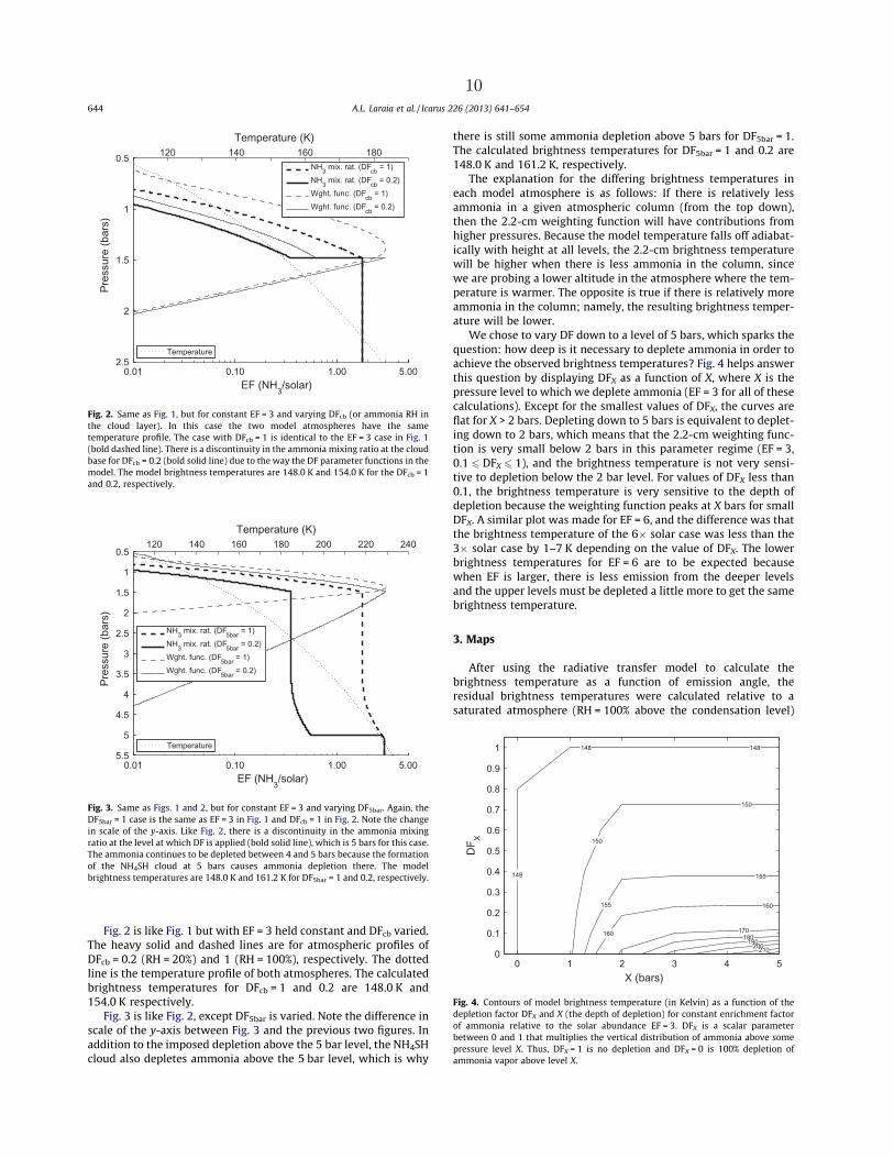
Fig. 2 is like Fig. 1 but with EF = 3 held constant and DFcb varied.The heavy solid and dashed lines are for atmospheric profiles ofDFcb = 0.2 (RH = 20%) and 1 (RH = 100%), respectively. The dottedline is the temperature profile of both atmospheres. The calculatedbrightness temperatures for DFcb = 1 and 0.2 are 148.0 K and154.0 K respectively.

Fig. 3 is like Fig. 2, except DF5bar is varied. Note the difference inscale of the y-axis between Fig. 3 and the previous two figures. Inaddition to the imposed depletion above the 5 bar level, the NH4SHcloud also depletes ammonia above the 5 bar level, which is why

there is still some ammonia depletion above 5 bars for DF5bar = 1.The calculated brightness temperatures for DF5bar = 1 and 0.2 are148.0 K and 161.2 K, respectively.

The explanation for the differing brightness temperatures ineach model atmosphere is as follows: If there is relatively lessammonia in a given atmospheric column (from the top down),then the 2.2-cm weighting function will have contributions fromhigher pressures. Because the model temperature falls off adiabat-ically with height at all levels, the 2.2-cm brightness temperaturewill be higher when there is less ammonia in the column, sincewe are probing a lower altitude in the atmosphere where the tem-perature is warmer. The opposite is true if there is relatively moreammonia in the column; namely, the resulting brightness temper-ature will be lower.

We chose to vary DF down to a level of 5 bars, which sparks thequestion: how deep is it necessary to deplete ammonia in order toachieve the observed brightness temperatures? Fig. 4 helps answerthis question by displaying DFX as a function of X, where X is thepressure level to which we deplete ammonia (EF = 3 for all of thesecalculations). Except for the smallest values of DFX, the curves areflat for X > 2 bars. Depleting down to 5 bars is equivalent to deplet-ing down to 2 bars, which means that the 2.2-cm weighting func-tion is very small below 2 bars in this parameter regime (EF = 3,0.1 6 DFX 6 1), and the brightness temperature is not very sensi-tive to depletion below the 2 bar level. For values of DFX less than0.1, the brightness temperature is very sensitive to the depth ofdepletion because the weighting function peaks at X bars for smallDFX. A similar plot was made for EF = 6, and the difference was thatthe brightness temperature of the 6 solar case was less than the3 solar case by 1–7 K depending on the value of DFX. The lowerbrightness temperatures for EF = 6 are to be expected becausewhen EF is larger, there is less emission from the deeper levelsand the upper levels must be depleted a little more to get the samebrightness temperature.

3. Maps

After using the radiative transfer model to calculate thebrightness temperature as a function of emission angle, theresidual brightness temperatures were calculated relative to asaturated atmosphere (RH = 100% above the condensation level)

0.01 0.10 1.00 5.00

0.5

1

1.5

2

2.5

EF (NH3/solar)

Pres

sure

(bar

s)

NH3 mix. rat. (DFcb = 1)NH3 mix. rat. (DFcb = 0.2)Wght. func. (DFcb = 1)Wght. func. (DFcb = 0.2)

120 140 160 180Temperature (K)

Temperature

Fig. 2. Same as Fig. 1, but for constant EF = 3 and varying DFcb (or ammonia RH inthe cloud layer). In this case the two model atmospheres have the sametemperature profile. The case with DFcb = 1 is identical to the EF = 3 case in Fig. 1(bold dashed line). There is a discontinuity in the ammonia mixing ratio at the cloudbase for DFcb = 0.2 (bold solid line) due to the way the DF parameter functions in themodel. The model brightness temperatures are 148.0 K and 154.0 K for the DFcb = 1and 0.2, respectively.

148

841841

150

150

155

155

160

160

170180

190200210

DF X

X (bars)0 1 2 3 4 5

0

0.1

0.2

0.3

0.4

0.5

0.6

0.7

0.8

0.9

1

Fig. 4. Contours of model brightness temperature (in Kelvin) as a function of thedepletion factor DFX and X (the depth of depletion) for constant enrichment factorof ammonia relative to the solar abundance EF = 3. DFX is a scalar parameterbetween 0 and 1 that multiplies the vertical distribution of ammonia above somepressure level X. Thus, DFX = 1 is no depletion and DFX = 0 is 100% depletion ofammonia vapor above level X.

0.01 0.10 1.00 5.00

0.5

1

1.5

2

2.5

3

3.5

4

4.5

5

5.5

EF (NH3/solar)

Pres

sure

(bar

s)

NH3 mix. rat. (DF5bar = 1)NH3 mix. rat. (DF5bar = 0.2)Wght. func. (DF5bar = 1)Wght. func. (DF5bar = 0.2)

120 140 160 180 200 220 240Temperature (K)

Temperature

Fig. 3. Same as Figs. 1 and 2, but for constant EF = 3 and varying DF5bar. Again, theDF5bar = 1 case is the same as EF = 3 in Fig. 1 and DFcb = 1 in Fig. 2. Note the changein scale of the y-axis. Like Fig. 2, there is a discontinuity in the ammonia mixingratio at the level at which DF is applied (bold solid line), which is 5 bars for this case.The ammonia continues to be depleted between 4 and 5 bars because the formationof the NH4SH cloud at 5 bars causes ammonia depletion there. The modelbrightness temperatures are 148.0 K and 161.2 K for DF5bar = 1 and 0.2, respectively.

644 A.L. Laraia et al. / Icarus 226 (2013) 641–654

10

model with the constituent enrichments given in Table 1. All futuremention of residual brightness temperatures refers to the residualsfrom this 3 solar ammonia reference model, which was chosenbased on the ability of the EF = 3 reference model to span the ob-served brightness temperatures better than the models with high-er or lower values of EF (Section 4, Figs. 11 and 12). Fig. 5 is a mapfrom December 9, 2009 of the 2.2-cm residual brightness temper-ature, created by the procedure explained in Section 3.2 of J13.There are four other maps analyzed in this work but not shownhere: September 23, 2005, October 13, 2009, July 25, 2010 andMarch 20, 2011. They are presented in Fig. 9 of J13.

3.1. Obstruction by the rings

An issue persistent throughout all the maps is that the equatoris obstructed by the rings (black region along equator in Fig. 5). Therings are optically thick scatterers with very little intrinsic thermalemission, and hence lower the measured brightness temperaturein the northern (southern) hemisphere when the spacecraft is be-low (above) the ring plane. When the spacecraft is in the ringplane, the ring inclination angle is exactly 0 and the rings disap-pear from view, allowing full view of the equator. Fig. 6 demon-strates the effect of the ring obstruction on brightnesstemperature for the July 2010 map, the map for which the effectof the rings is most prominent (see Fig. 9 of J13). Each line is a dif-ferent meridional (pole-to-pole) scan near the spacecraft’s ringplane crossing (RPC), labeled with the ring inclination angle. Foran example of a RPC scan see Fig. 5 near longitude 18W, wherethe ring blockage at the equator goes to zero. During the July2010 observation period, Cassini was moving rapidly across thering plane. Thus the effect of the rings on the brightness tempera-ture is large, 50% between two scans taken only minutes apart (e.g.from scan 0.019 to 0.377). Fig. 6 demonstrates that ring incli-nation angles as small as 0.1 have large effects on the observedequatorial brightness temperature.

Cassini crossed the ring plane in four of the five maps. We testour ability to remove the ring effect with a model that assumes anisothermal (150 K) brightness temperature for the atmosphere anda ring brightness temperature of 25 K. With this model wesynthesize the individual brightness scans taking into accountthe actual geometry of the spacecraft and the instrument. The rightpanel of Fig. 7 shows the results from this model for the four scans

closest to RPC for the December 2009 map, which has the smallestring inclination angle while observing the equator. The labels arethe same as in Fig. 6, but the scales along the y-axis are different.The left panel shows the observed brightness temperatures forthe same scans. The model does not predict any dip in brightnesstemperature at the equator for the RPC scan (0.001 ringinclination angle), demonstrating that we are observing the trueequatorial brightness temperature in this scan. In the left panel,the 0.001 scan is continuously flat through the equator (within±2), which does not occur for any other RPC scan except for the

Fig. 5. 2.2-cm residual brightness temperature (in Kelvin) map of Saturn from December 9, 2009. The residual temperature is calculated by subtracting the brightnesstemperature from a fully-saturated reference model with 3 solar ammonia mixing ratio (Section 2) from the observed brightness temperature. The black band at the equatoris due to the cold rings obstructing the atmosphere. Section 3.2 of J13 offers a detailed explanation of how the brightness temperature maps were generated.

-4 -2 0 2 4Planetographic Latitude (degrees)

70

80

90

100

110

120

130

140

150

Brig

htne

ss T

empe

ratu

re (K

)

0.318o

0.152o

-0.019o

-0.197o

-0.377o

Fig. 6. Five individual scans around ring plane crossing (RPC) for the July 2010 map.Scans are labeled with their ring inclination angles as viewed by Cassini. The firstscan, labeled 0.318, was made while the spacecraft was in the southernhemisphere, therefore the ring blockage occurred in the northern hemisphere. AsCassini approached the ring plane, the effect of the rings became quite small.Because the spacecraft was moving fairly quickly across the ring plane in this map,the rings had a very large effect from one scan to the next.

A.L. Laraia et al. / Icarus 226 (2013) 641–654 645

11

September 2005 scan, which is at very low resolution comparedwith the other three maps (Fig. 8). Thus we take the DecemberRPC scan as the RPC scan that provides the true equatorial bright-ness temperature. The increase in brightness temperature at lati-tudes greater than 3 in both hemispheres is not in the modelbut is a real property of Saturn’s atmosphere.

Fig. 8 displays residual brightness temperatures versus latitudefor all four RPC scans. The scale along the y-axis is expandedrelative to that in Figs. 6 and 7. The ring inclination angles for eachscan are displayed in parentheses in the legend. The segment of the

September 2005 map where the RPC occurred is at very low reso-lution (Fig. 9, J13), and is therefore affected by the two bright bandsat ±9 with a contribution of about +0.7 K. Applying this correctionto the September 2005 scan brings the residual brightness temper-ature down to 0.5 K at the equator. The observed residuals are con-sistent with 1 K variability in the equatorial region. We chose theDecember 2009 RPC scan to represent the equatorial brightnesstemperature for all five maps in Fig. 9 because it has the bestgeometry (lowest inclination at RPC) and produces the best pictureof the equatorial brightness temperature that we have.

-4 -2 0 2 4Planetographic Latitude (degrees)

142

144

146

148

150

Brig

htne

ss T

empe

ratu

re (K

)

0.044o

0.029o

0.015o

0.001o

-4 -2 0 2 4Planetographic Latitude (degrees)

142

144

146

148

150

0.044o

0.029o

0.015o

0.001o

Fig. 7. Left panel: Same as Fig. 6 for the December 2009 map. The RPC scan for this map has the smallest ring inclination angle of all the maps (while viewing the equator),and is flat across the equator. This is the best view of the equatorial brightness temperature that we have of all five maps. Right panel: Same labeling, but for a simple beamconvolution model that takes into account the Cassini–Saturn geometry and includes the A and B rings only. It assumes an isothermal atmosphere of 150 K, and takes themicrowave brightness of both the A and B rings to be 25 K. According to this model, we actually see the equator with no ring blockage for the 0.001 scan.

-4 -2 0 2 4Planetographic Latitude (degrees)

-2

0

2

4

Res

idua

l Brig

htne

ss T

empe

ratu

re (K

) Sept 23, 2005 (0.01)Dec 9, 2009 (0.001)Oct 13, 2009 (-0.007)July 25, 2010 (-0.019)

Fig. 8. Residual brightness temperatures for RPC scans of the four maps and theiraverage. The ring inclination angle for each scan is in parentheses next to the date.Because of the low resolution of the September 2005 scan, the bright bands off theequator affect the equatorial brightness temperature, causing it to be 0.7 K too high.With this in mind, the four scans are within ±1.5 K. The December 2009 RPC scan isflat across the equator with a very small ring inclination angle. Thus it provides thetrue equatorial brightness temperature.

-60 -40 -20 0 20 40 60Planetographic Latitude (degrees)

0

1

2

3

4

5

6

Res

idua

l Brig

htne

ss T

empe

ratu

re (K

)

0

1

2

3

4

5

6

Standard Deviation of Brightness

Temperature (K)

Fig. 9. Mean residual brightness temperature (open circle and + signs) and its meanstandard deviation as a function of planetographic latitude (solid line) for all fivemaps, excluding the northern storm and the latitudes near the equator where therings block the view of the atmosphere. Observations were sorted into latitude bins0.4 wide since the latitudes are unevenly spaced. From 4 to +4 the singleDecember 2009 RPC scan is used (+ signs), because it is the best view of theequatorial brightness temperature that we have of all the maps (Section 3.1).Standard deviations were calculated at each latitude for each map and thenaveraged. The average is weighted by the number of observations at a given latitudeand date and the sum is over all five observation dates.

646 A.L. Laraia et al. / Icarus 226 (2013) 641–654

12

3.2. General features

With the exception of the March 2011 map, which has the2010–2011 northern storm (Figs. 9 and 12, J13) or great white spot(Fischer et al., 2011; Sánchez-Lavega et al., 2011), all of the mapsshare the same general characteristics. In what follows, all lati-tudes are planetographic unless explicitly stated. In Fig. 5, theequatorial region, within 10 of the equator, is texturally anoma-lous compared with the rest of the map, even when excludingthe effect of the rings. There is non-uniform high brightness near9 and 9 that generally decreases towards the equator, whichis obstructed by the rings for all scans except for the one duringRPC. The brightness temperature variations on the maps are quitelarge, with variations of more than 10 K, and we investigate thecauses of these variations. There are some structures in the south-ern hemisphere band between 42 and 47 (e.g. at 340W and75W in Fig. 5), which is just south of the westward jet at 42(35 planetocentric) and has been the site of many lightningobservations (Dyudina et al., 2007; Fischer et al., 2011). There arealso two narrow bright bands at 33 and 37, and a broad darkband from 15 to 30.

The highest brightness temperature in the northern storm is165.7 K (18.9 K residual brightness temperature). The highestbrightness temperature in all five maps is 167.1 K (19.3 K residualbrightness temperature), which occurs in the subtropical latitudesin the October 2009 map.

Fig. 9 shows the zonally averaged residual brightness tempera-ture (open circles and + signs) and its standard deviation (solidline) as a function of latitude. Outside of ±4 latitude, the bright-ness temperatures are averaged over longitude and over all fivemaps (open circles), excluding the 2010–2011 northern stormand the latitudes near the equator where the rings block the viewof the atmosphere. Within ±4 of the equator, a single RPC scanfrom the December 2009 map is used (+ symbols), as explainedin Section 3.1. The standard deviation was computed with respectto longitude for each latitude outside ±4, and then the weightedstandard deviation for all five maps was calculated. The weightsused in this calculation are the number of observations at a givenlatitude and date and the sum is over all five observation dates.The globally averaged residual brightness temperature fromFig. 9 is 1.7 ± 1.1 K, where the 1.1 K is real variability of the longi-tudinally-averaged brightnesses in Saturn’s atmosphere.

The residual brightness temperatures shown in Fig. 9 are posi-tive at every latitude. One important implication of this observa-tion is that the atmosphere is always ammonia-depleted withrespect to a fully-saturated 3 solar ammonia model (Table 1). Astriking feature of Fig. 9 is the two relatively bright bands near±9, the subtropics of Saturn, with residuals of 3.8 K and 5.8 K inthe southern and northern hemispheres, respectively (correspond-ing to brightness temperatures of 151.7 K and 153.7 K). These twobright latitudes surround a relatively low residual brightness tem-perature of 0.1 K (corresponding to a brightness temperature of148.1 K) at the equator. At the equator the atmosphere is close tobeing saturated with ammonia. The subtropical bands are accom-panied by elevated standard deviation, indicating that there issome structure in these regions. Another feature is the pair ofbright bands around 36 and 34 with averaged residuals of2.5 and 3.6 K respectively (corresponding to brightness tempera-tures of 149.2 and 150.5 K), which correspond to the two narrowbands in the southern hemisphere in Fig. 5. There are two regionswith high standard deviation in the southern hemisphere, one near33 (28 planetocentric) and the other near 43 (37 plane-tocentric). The latter is the latitude of storm alley and the site ofthe southern hemisphere lightning (Dyudina et al., 2007). The rel-atively high standard deviation in storm alley corresponds to thebright dots seen there (Fig. 5, longitude 345W), which are likely

to be holes in the ammonia layer associated with the holes in theclouds described by Dyudina et al. (2007). Dyudina et al. (in prep-aration) investigates the structure of these southern hemispherestorms and presents the lightning observations from both thesouthern storms and the 2010–2011 northern storm. The northernlatitudes have relatively constant brightness temperatures, withfluctuations on the order of 1 K from latitude to latitude. Thesouthern hemisphere has larger brightness temperature gradientsthan the northern hemisphere, for example almost a 4 K increasefrom 25 to 35. For the northern storm (not included inFig. 9), the standard deviation in the latitude band between 20and 50 is much larger, reaching a peak value of 6 K at 40.

When looking at the relatively bright spots within the brightsubtropical bands in all five maps, it is natural to ask if there isany periodic structure in these regions. Jupiter, for example, hadthe equatorial plumes in the northern hemisphere with longitudinalwavenumber between 11 and 13 at the time of the Voyager encoun-ters (Allison, 1990), and between 8 and 12 determined more re-cently (Arregi et al., 2006). To determine whether there is periodicstructure in the subtropical bands of Saturn, we calculated the auto-correlation of the brightness temperature with respect to longitudefor latitude bands between 6 and 10 in both hemispheres. We usedbinning to remedy the problems that arise due to unevenly spacedobservation points and large gaps in the maps. For a given latitude,every pair of points was placed into a bin 3 wide based on the lagbetween the points. Thus the 0 lag bin has pairs of points with lagsfrom 0 to 3. The next bin is 3–6, and so on. We did this for fourmaps, excluding the July 2010 map because the rings obstruct themajority of the subtropical bands. The resulting averaged correla-tion coefficients are plotted versus longitudinal lag in Fig. 10. Thecorrelations in the southern hemisphere tend to fall off more rapidlythan in the northern hemisphere, with the exception of the Decem-ber 2009 map. This indicates that the bright spots in the northernhemisphere subtropical band have a greater longitudinal span thanthose in the southern hemisphere. Four of the eight panels in Fig. 10reveal wave-like features with longitudinal periods ranging from20 to 45 (zonal wavenumbers 18–8, respectively) for the 610latitude range. The period varies from year to year, and there is noindication of a recurring dominant period. We did not find anywave-like features in other latitude ranges.

4. Comparison with radiative transfer model

Ammonia vapor is the only effective source of opacity in Sat-urn’s atmosphere at 2.2-cm wavelength, as shown by Fig. 3 ofJ13 that plots absorption coefficient versus height for the relevantconstituents. Ammonia is by far the dominant absorber in our sen-sitivity range. Thus the 2.2-cm brightness temperature maps yieldinformation about the ammonia vapor distribution. To interpretthe maps we used the JAMRT program described in Section 2 tocalculate 2.2-cm brightness temperatures based on different verti-cal profiles of ammonia. We varied two parameters, EF and DF, alsodescribed in Section 2.

Figs. 1 and 2 suggest that we cannot get brightness temperaturevariations larger than 11 K by varying only EF (ammonia deepabundance) or DFcb (ammonia RH in the cloud layer), since thesetwo parameters only account for brightness temperature varia-tions of up to 11 K. Fig. 11 demonstrates this by displaying themodel brightness temperature (in Kelvin) as a function of DFcb

(or RH) and EF. All the calculations done in Figs. 11 and 12 weredone at an emission angle of 0. This is important to note becausethe model brightness temperatures decrease with increasing emis-sion angle due to limb darkening. For example, a brightness tem-perature of 160 K at the equator would have a residual of 12 K,while a brightness temperature of 160 K at 40 (e.g., the 2010–2011 northern storm) would have a residual of 13.5 K.

A.L. Laraia et al. / Icarus 226 (2013) 641–654 647

13

In Fig. 11, as expected, the brightness temperatures increasewith decreasing DFcb (decreasing RH), since depletion of ammoniapushes the weighting function deeper into the atmosphere whereit is warmer. However, as mentioned above, the largest tempera-ture contrast that can be obtained in this parameter regime is11 K (148–159 K, Fig. 11), which indicates that ammonia vapormust be depleted to levels deeper than the ammonia cloud in orderto achieve the highest brightness temperatures seen in the maps(160+ K), provided that DFcb > 0.1. If DFcb < 0.1, then the ammoniaconcentration in the cloud region is almost zero, which is unlikelygiven ammonia concentrations reported by Fletcher et al. (2011a)for the 1–4 bar region. The idea that the formation of the NH4SHcloud around 5 bars is the ammonia-depletion mechanism beneaththe ammonia-ice cloud has been discussed by previous authors(e.g. Briggs and Sackett, 1989). Since our model includes the forma-tion of this cloud (with H2S enriched by 5 solar, Table 1), ammo-nia must be depleted even more than just by the NH4SH cloudformation in order to agree with observations, unless H2S is in real-ity enriched by more than 5 solar on Saturn.

There is a trend of increasing brightness with increasing EF atlow DFcb in Fig. 11. This is counter-intuitive, because increasingEF means more ammonia, but it is an artifact of the model andhas an explanation. The DFcb parameter depletes ammonia downto the ammonia cloud base, and for very low DFcb that is wherethe weighting function peaks. As EF increases, the ammonia cloudbase moves to deeper (and warmer) levels (Fig. 1), bringing theweighting function with it. The effect of lowering the altitude ofthe weighting function outweighs the effect of adding ammoniaat deeper levels, and brightness temperature increases withincreasing EF.

Fig. 12 is the same as Fig. 11, but for DF5bar. Note that the con-tour interval has been increased from 1 to 4 K. As expected, thebrightness temperature increases with decreasing DF5bar anddecreasing EF. By depleting the ammonia down to this deeper level(5 bars), we are able to achieve the 166–167 K brightness temper-atures seen in the maps. This requires either DFcb < 0.1 (Fig. 11,lower right portion) or a combination of DF5bar < 0.3 and EF < 4(Fig. 12, lower left corner). Figs. 11 and 12 are for rays propagating

0 20 40 60 80 100-1.0

-0.5

0.0

0.5

1.0C

orre

latio

n C

oeffi

cien

t

6 - 10o Sept 2005

0 20 40 60 80 100-1.0

-0.5

0.0

0.5

1.0-6 - -10o Sept 2005

0 20 40 60 80 100-1.0

-0.5

0.0

0.5

1.0

Cor

rela

tion

Coe

ffici

ent

6 - 10o Oct 2009

0 20 40 60 80 100-1.0

-0.5

0.0

0.5

1.0-6 - -10o Oct 2009

0 20 40 60 80 100-1.0

-0.5

0.0

0.5

1.0

Cor

rela

tion

Coe

ffici

ent

6 - 10o Dec 2009

0 20 40 60 80 100-1.0

-0.5

0.0

0.5

1.0-6 - -10o Dec 2009

0 20 40 60 80 100

Lag (Degrees Longitude)

-1.0

-0.5

0.0

0.5

1.0

Cor

rela

tion

Coe

ffici

ent

6 - 10o March 2011

0 20 40 60 80 100

Lag (Degrees Longitude)

-1.0

-0.5

0.0

0.5

1.0-6 - -10o March 2011

Fig. 10. Autocorrelations of brightness temperature with respect to longitude versus longitudinal lag. The panels display averages of the autocorrelations in the latitudebands from 6 to 10 in the northern hemisphere (left column) and the southern hemisphere (right column) for each map, excluding the July 2010 map due to the largeamount of ring blockage in the subtropics.

648 A.L. Laraia et al. / Icarus 226 (2013) 641–654

14

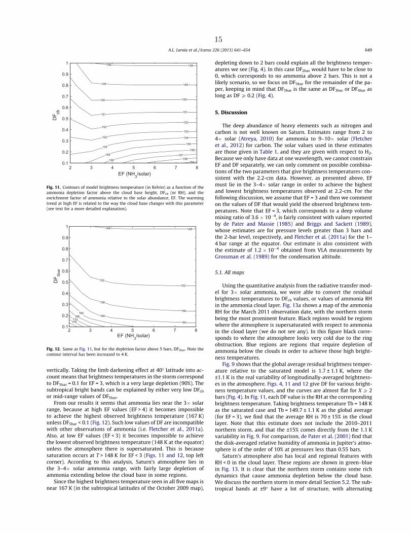
vertically. Taking the limb darkening effect at 40 latitude into ac-count means that brightness temperatures in the storm correspondto DF5bar = 0.1 for EF = 3, which is a very large depletion (90%). Thesubtropical bright bands can be explained by either very low DFcb

or mid-range values of DF5bar.From our results it seems that ammonia lies near the 3 solar

range, because at high EF values (EF > 4) it becomes impossibleto achieve the highest observed brightness temperature (167 K)unless DF5bar < 0.1 (Fig. 12). Such low values of DF are incompatiblewith other observations of ammonia (i.e. Fletcher et al., 2011a).Also, at low EF values (EF < 3) it becomes impossible to achievethe lowest observed brightness temperature (148 K at the equator)unless the atmosphere there is supersaturated. This is becausesaturation occurs at T > 148 K for EF < 3 (Figs. 11 and 12, top leftcorner). According to this analysis, Saturn’s atmosphere lies inthe 3–4 solar ammonia range, with fairly large depletion ofammonia extending below the cloud base in some regions.

Since the highest brightness temperature seen in all five maps isnear 167 K (in the subtropical latitudes of the October 2009 map),

depleting down to 2 bars could explain all the brightness temper-atures we see (Fig. 4). In this case DF2bar would have to be close to0, which corresponds to no ammonia above 2 bars. This is not alikely scenario, so we focus on DF5bar for the remainder of the pa-per, keeping in mind that DF5bar is the same as DF3bar or DF4bar aslong as DF P 0.2 (Fig. 4).

5. Discussion

The deep abundance of heavy elements such as nitrogen andcarbon is not well known on Saturn. Estimates range from 2 to4 solar (Atreya, 2010) for ammonia to 9–10 solar (Fletcheret al., 2012) for carbon. The solar values used in these estimatesare those given in Table 1, and they are given with respect to H2.Because we only have data at one wavelength, we cannot constrainEF and DF separately, we can only comment on possible combina-tions of the two parameters that give brightness temperatures con-sistent with the 2.2-cm data. However, as presented above, EFmust lie in the 3–4 solar range in order to achieve the highestand lowest brightness temperatures observed at 2.2-cm. For thefollowing discussion, we assume that EF = 3 and then we commenton the values of DF that would yield the observed brightness tem-peratures. Note that EF = 3, which corresponds to a deep volumemixing ratio of 3.6 104, is fairly consistent with values reportedby de Pater and Massie (1985) and Briggs and Sackett (1989),whose estimates are for pressure levels greater than 3 bars andthe 2-bar level, respectively, and Fletcher et al. (2011a) for the 1–4 bar range at the equator. Our estimate is also consistent withthe estimate of 1.2 104 obtained from VLA measurements byGrossman et al. (1989) for the condensation altitude.

5.1. All maps

Using the quantitative analysis from the radiative transfer mod-el for 3 solar ammonia, we were able to convert the residualbrightness temperatures to DFcb values, or values of ammonia RHin the ammonia cloud layer. Fig. 13a shows a map of the ammoniaRH for the March 2011 observation date, with the northern stormbeing the most prominent feature. Black regions would be regionswhere the atmosphere is supersaturated with respect to ammoniain the cloud layer (we do not see any). In this figure black corre-sponds to where the atmosphere looks very cold due to the ringobstruction. Blue regions are regions that require depletion ofammonia below the clouds in order to achieve those high bright-ness temperatures.

Fig. 9 shows that the global average residual brightness temper-ature relative to the saturated model is 1.7 ± 1.1 K, where the±1.1 K is the real variability of longitudinally-averaged brightness-es in the atmosphere. Figs. 4, 11 and 12 give DF for various bright-ness temperature values, and the curves are almost flat for X P 2bars (Fig. 4). In Fig. 11, each DF value is the RH at the correspondingbrightness temperature. Taking brightness temperature Tb = 148 Kas the saturated case and Tb = 149.7 ± 1.1 K as the global average(for EF = 3), we find that the average RH is 70 ± 15% in the cloudlayer. Note that this estimate does not include the 2010–2011northern storm, and that the ±15% comes directly from the 1.1 Kvariability in Fig. 9. For comparison, de Pater et al. (2001) find thatthe disk-averaged relative humidity of ammonia in Jupiter’s atmo-sphere is of the order of 10% at pressures less than 0.55 bars.

Saturn’s atmosphere also has local and regional features withRH < 0 in the cloud layer. These regions are shown in green–bluein Fig. 13. It is clear that the northern storm contains some richdynamics that cause ammonia depletion below the cloud base.We discuss the northern storm in more detail Section 5.2. The sub-tropical bands at ±9 have a lot of structure, with alternating

148 148

149 149

150 150

151151

152152

153

153

154

154

155

155

156

156

157158

159

cb

EF (NH

DF

3/solar)2 3 4 5 6 7 8

0.1

0.2

0.3

0.4

0.5

0.6

0.7

0.8

0.9

1

Fig. 11. Contours of model brightness temperature (in Kelvin) as a function of theammonia depletion factor above the cloud base height, DFcb (or RH), and theenrichment factor of ammonia relative to the solar abundance, EF. The warmingtrend at high EF is related to the way the cloud base changes with this parameter(see text for a more detailed explanation).

148 148

152

152

156

156

160

160

164168

172176

DF 5b

ar

EF (NH3/solar)2 3 4 5 6 7 8

0.1

0.2

0.3

0.4

0.5

0.6

0.7

0.8

0.9

1

Fig. 12. Same as Fig. 11, but for the depletion factor above 5 bars, DF5bar. Note thecontour interval has been increased to 4 K.

A.L. Laraia et al. / Icarus 226 (2013) 641–654 649

15

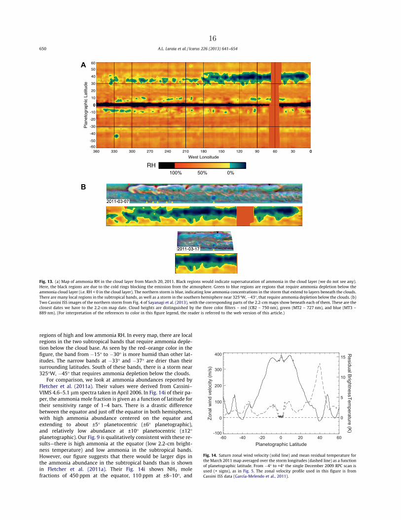
regions of high and low ammonia RH. In every map, there are localregions in the two subtropical bands that require ammonia deple-tion below the cloud base. As seen by the red–orange color in thefigure, the band from 15 to 30 is more humid than other lat-itudes. The narrow bands at 33 and 37 are drier than theirsurrounding latitudes. South of these bands, there is a storm near325W, 45 that requires ammonia depletion below the clouds.

For comparison, we look at ammonia abundances reported byFletcher et al. (2011a). Their values were derived from Cassini–VIMS 4.6–5.1 lm spectra taken in April 2006. In Fig. 14i of their pa-per, the ammonia mole fraction is given as a function of latitude fortheir sensitivity range of 1–4 bars. There is a drastic differencebetween the equator and just off the equator in both hemispheres,with high ammonia abundance centered on the equator andextending to about ±5 planetocentric (±6 planetographic),and relatively low abundance at ±10 planetocentric (±12planetographic). Our Fig. 9 is qualitatively consistent with these re-sults—there is high ammonia at the equator (low 2.2-cm bright-ness temperature) and low ammonia in the subtropical bands.However, our figure suggests that there would be larger dips inthe ammonia abundance in the subtropical bands than is shownin Fletcher et al. (2011a). Their Fig. 14i shows NH3 molefractions of 450 ppm at the equator, 110 ppm at ±8–10, and

A

B

Fig. 13. (a) Map of ammonia RH in the cloud layer from March 20, 2011. Black regions would indicate supersaturation of ammonia in the cloud layer (we do not see any).Here, the black regions are due to the cold rings blocking the emission from the atmosphere. Green to blue regions are regions that require ammonia depletion below theammonia cloud layer (i.e. RH < 0 in the cloud layer). The northern storm is blue, indicating low ammonia concentrations in the storm that extend to layers beneath the clouds.There are many local regions in the subtropical bands, as well as a storm in the southern hemisphere near 325W, 43, that require ammonia depletion below the clouds. (b)Two Cassini ISS images of the northern storm from Fig. 4 of Sayanagi et al. (2013), with the corresponding parts of the 2.2-cm maps show beneath each of them. These are theclosest dates we have to the 2.2-cm map date. Cloud heights are distinguished by the three color filters – red (CB2 – 750 nm), green (MT2 – 727 nm), and blue (MT3 –889 nm). (For interpretation of the references to color in this figure legend, the reader is referred to the web version of this article.)

-60 -40 -20 0 20 40 60Planetographic Latitude

-100

0

100

200

300

400

Zona

l win

d ve

loci

ty (m

/s)

0

5

10

15

Residual BrightnessTem

perature (K)

Fig. 14. Saturn zonal wind velocity (solid line) and mean residual temperature forthe March 2011 map averaged over the storm longitudes (dashed line) as a functionof planetographic latitude. From 4 to +4 the single December 2009 RPC scan isused (+ signs), as in Fig. 5. The zonal velocity profile used in this figure is fromCassini ISS data (García-Melendo et al., 2011).

650 A.L. Laraia et al. / Icarus 226 (2013) 641–654

16

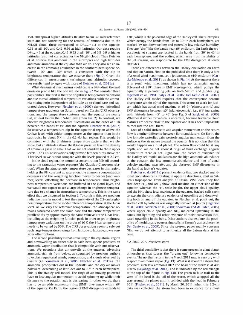
150–200 ppm at higher latitudes. Relative to our 3 solar referencestate and not correcting for the removal of ammonia due to theNH4SH cloud, these correspond to DF5bar = 1.3 at the equator,0.31 at ±8–10, and 0.42–0.56 at high latitudes. Our data requireDF5bar = 1 at the equator, 0.45–0.55 at ±8–10 and 0.8–0.9 at higherlatitudes (also not correcting for the NH4SH cloud). Thus Fletcheret al. observe less ammonia in the subtropics and high latitudesand more ammonia at the equator than we do. They also see an in-crease in the ammonia abundance in the southern hemisphere be-tween 20 and 30 which is consistent with the dip inbrightness temperature that we observe there (Fig. 9). Given thedifferences in measurement techniques and altitudes covered,our results tend to agree with those of Fletcher et al. (2011a).

What dynamical mechanisms could cause a latitudinal thermalemission profile like the one we see in Fig. 9? We consider threepossibilities. The first is that the brightness temperature variationsare due to real latitudinal temperature variations, with the ammo-nia mixing ratio independent of latitude up to cloud base and sat-urated above. However, Fletcher et al. (2007) derived latitudinaltemperature gradients on Saturn based on Cassini/CIRS observa-tions, and the temperature contours near the equator are nearlyflat, at least below the 0.5-bar level (their Fig. 2). In contrast, weobserve brightness temperature fluctuations on the order of 10 Kbetween the bands at ±9 and the equator. Fletcher et al. (2007)do observe a temperature dip in the equatorial region above the0.4 bar level, with colder temperatures at the equator than in thesubtropics by about 5 K in the 0.2–0.4 bar region. This would beconsistent with the brightness temperature pattern that we ob-serve, but at altitudes above the 0.4-bar pressure level the densityof ammonia gas is so small that we are not sensitive to these upperlevels. The CIRS observations only provide temperatures above the1 bar level so we cannot compare with the levels probed at 2.2 cm.

In the cloud region, the ammonia concentration falls off accord-ing to the saturation vapor pressure (the Clausius–Clapeyron rela-tion). When the atmospheric temperature decreases in this region,holding the RH constant at saturation, the ammonia concentrationdecreases and the weighting function moves to deeper (and war-mer) levels, offsetting the decrease in temperature. Thus bright-ness temperature variations are buffered in the cloud layer, andwe would not expect to see a large change in brightness tempera-ture due to a change in atmospheric temperature. This is the sameeffect that we discussed in Section 2. To confirm this, we used ourradiative transfer model to test the sensitivity of the 2.2-cm bright-ness temperature to the model reference temperature at the 1-barlevel. As we vary the reference temperature, the atmosphere re-mains saturated above the cloud base and the entire temperatureprofile shifts by approximately the same value as at the 1-bar level,including at the weighting function peak. In order to get brightnesstemperature variations on the order of 10 K, the 1-bar temperatureneeds to be varied by 50 K. The CIRS observations seem to rule outsuch large temperature swings from latitude to latitude, so we con-sider other options.

The second possibility is that upwelling in the equatorial regionand downwelling on either side in each hemisphere produces anammonia vapor distribution that is compatible with our observa-tions. We postulate that air upwells at the equator, advectingammonia-rich air from below, as suggested by previous authorsto explain equatorial winds, composition, and clouds observed byCassini (i.e. Yamakazi et al., 2005; Fletcher et al., 2011a). Theammonia precipitates out in the updrafts, and the dry air movespoleward, descending at latitudes out to ±9 in each hemisphere.This is the Hadley cell model. The rings of air moving polewardhave to lose angular momentum to avoid spinning up while theirdistance to the rotation axis is decreasing. In other words, therehas to be an eddy momentum flux (EMF) divergence within ±9of the equator. On Earth, the region of EMF divergence extends to

±30, which is the poleward edge of the Hadley cell. The subtropics,which occupy the bands from 10 to 30 in each hemisphere, aremarked by net downwelling and generally low relative humidity.They are ‘‘dry,’’ like the bands near ±9 on Saturn. On Earth the tro-pospheric jet streams are located in the bands from 30 to 40 ineach hemisphere, and the eddies, which arise from instability ofthe jet streams, are responsible for the EMF divergence at lowerlatitudes.

There are differences between the Hadley circulation on Earthand that on Saturn. First, in the published data there is only a hintof a zonal wind maximum, i.e., a jet stream, at ±10 on Saturn (Gar-cía-Melendo et al., 2011), as shown in Fig. 14. At the equator thereis a zonal wind maximum, which has no terrestrial analog.Poleward of ±10 there is EMF convergence, which pumps theequatorially superrotating jets on both Saturn and Jupiter (e.g.Ingersoll et al., 1981; Salyk et al., 2006; Del Genio et al., 2007).The Hadley cell model requires that the convergence becomedivergence within ±9 of the equator. This seems to work for Jupi-ter, which has zonal wind maxima at ±6–7 (planetocentric) andEMF divergence between ±5 (planetocentric), i.e., u0v 0 increasingwith latitude from 5 to +5 (see Fig. 5 of Salyk et al., 2006).Whether it works for Saturn is uncertain, because trackable cloudfeatures are scarce close to the equator and it has been impossibleto measure the EMF there.

Lack of a solid surface to add angular momentum on the returnflow is another difference between Earth and Saturn. On Earth, thelow latitude easterlies gain westerly angular momentum from thesurface as the air moves toward the equator. It is not clear that thiswould happen on a fluid planet. The return flow could be at anydepth, and we do not know if rings of fluid exchange angularmomentum there or not. Right now, the pieces of evidence forthe Hadley cell model on Saturn are the high ammonia abundanceat the equator, the low ammonia abundance and hint of zonalvelocity maxima near ±9, and the observed EMF divergence inthe band at Jupiter’s equator.

Fletcher et al. (2011a) present evidence that two stacked merid-ional circulation cells, rotating in opposite directions, exist in Sat-urn’s troposphere. From analysis of Cassini VIMS data, they findthat deep PH3 and AsH3 show local maxima on either side of theequator, whereas the PH3 scale height, the upper cloud opacity,and the NH3 show local maxima at the equator. Stacked cells seemto explain the contradictory evidence of upwelling and downwel-ling both on and off the equator. As Fletcher et al. point out, thestacked cell hypothesis was originally invoked at Jupiter (Ingersollet al., 2000; Gierasch et al., 2000; Showman and de Pater, 2005),where upper cloud opacity and NH3 indicated upwelling in thezones, but lightning and other evidence of moist convection indi-cated upwelling in the belts. Other authors also explore the possi-bility of meridionally overturning cells in Saturn’s atmosphere (i.e.Del Genio et al., 2009). Since the present paper mainly concernsNH3, we do not attempt to synthesize all the Saturn data at thistime.

5.2. 2010–2011 Northern storm

The third possibility is that there is some process in giant planetatmospheres that causes the ‘‘drying out’’ following convectiveevents. The northern storm in the March 2011 map is very dry withrespect to ammonia vapor (Fig. 13). What is it about the storm thatproduces such low ammonia RH? The head of the storm is at 40,180W (Sayanagi et al., 2013), and is indicated by the red triangleat the top of the figure in Fig. 13b. The green to blue trail to thewest of the head is the tail of the storm, which wrapped all theway around the planet until it collided with the head in February2011 (Fischer et al., 2011). By March 20, 2011, when this 2.2-cmdata was collected, the storm had been in existence for almost

A.L. Laraia et al. / Icarus 226 (2013) 641–654 651

17

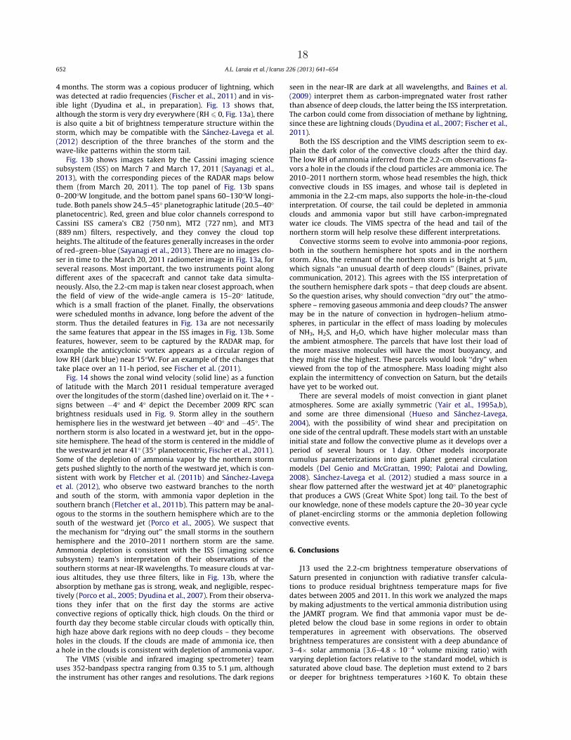
4 months. The storm was a copious producer of lightning, whichwas detected at radio frequencies (Fischer et al., 2011) and in vis-ible light (Dyudina et al., in preparation). Fig. 13 shows that,although the storm is very dry everywhere (RH 6 0, Fig. 13a), thereis also quite a bit of brightness temperature structure within thestorm, which may be compatible with the Sánchez-Lavega et al.(2012) description of the three branches of the storm and thewave-like patterns within the storm tail.

Fig. 13b shows images taken by the Cassini imaging sciencesubsystem (ISS) on March 7 and March 17, 2011 (Sayanagi et al.,2013), with the corresponding pieces of the RADAR maps belowthem (from March 20, 2011). The top panel of Fig. 13b spans0–200W longitude, and the bottom panel spans 60–130W longi-tude. Both panels show 24.5–45 planetographic latitude (20.5–40planetocentric). Red, green and blue color channels correspond toCassini ISS camera’s CB2 (750 nm), MT2 (727 nm), and MT3(889 nm) filters, respectively, and they convey the cloud topheights. The altitude of the features generally increases in the orderof red–green–blue (Sayanagi et al., 2013). There are no images clo-ser in time to the March 20, 2011 radiometer image in Fig. 13a, forseveral reasons. Most important, the two instruments point alongdifferent axes of the spacecraft and cannot take data simulta-neously. Also, the 2.2-cm map is taken near closest approach, whenthe field of view of the wide-angle camera is 15–20 latitude,which is a small fraction of the planet. Finally, the observationswere scheduled months in advance, long before the advent of thestorm. Thus the detailed features in Fig. 13a are not necessarilythe same features that appear in the ISS images in Fig. 13b. Somefeatures, however, seem to be captured by the RADAR map, forexample the anticyclonic vortex appears as a circular region oflow RH (dark blue) near 15W. For an example of the changes thattake place over an 11-h period, see Fischer et al. (2011).

Fig. 14 shows the zonal wind velocity (solid line) as a functionof latitude with the March 2011 residual temperature averagedover the longitudes of the storm (dashed line) overlaid on it. The + -signs between 4 and 4 depict the December 2009 RPC scanbrightness residuals used in Fig. 9. Storm alley in the southernhemisphere lies in the westward jet between 40 and 45. Thenorthern storm is also located in a westward jet, but in the oppo-site hemisphere. The head of the storm is centered in the middle ofthe westward jet near 41 (35 planetocentric, Fischer et al., 2011).Some of the depletion of ammonia vapor by the northern stormgets pushed slightly to the north of the westward jet, which is con-sistent with work by Fletcher et al. (2011b) and Sánchez-Lavegaet al. (2012), who observe two eastward branches to the northand south of the storm, with ammonia vapor depletion in thesouthern branch (Fletcher et al., 2011b). This pattern may be anal-ogous to the storms in the southern hemisphere which are to thesouth of the westward jet (Porco et al., 2005). We suspect thatthe mechanism for ‘‘drying out’’ the small storms in the southernhemisphere and the 2010–2011 northern storm are the same.Ammonia depletion is consistent with the ISS (imaging sciencesubsystem) team’s interpretation of their observations of thesouthern storms at near-IR wavelengths. To measure clouds at var-ious altitudes, they use three filters, like in Fig. 13b, where theabsorption by methane gas is strong, weak, and negligible, respec-tively (Porco et al., 2005; Dyudina et al., 2007). From their observa-tions they infer that on the first day the storms are activeconvective regions of optically thick, high clouds. On the third orfourth day they become stable circular clouds with optically thin,high haze above dark regions with no deep clouds – they becomeholes in the clouds. If the clouds are made of ammonia ice, thena hole in the clouds is consistent with depletion of ammonia vapor.

The VIMS (visible and infrared imaging spectrometer) teamuses 352-bandpass spectra ranging from 0.35 to 5.1 lm, althoughthe instrument has other ranges and resolutions. The dark regions

seen in the near-IR are dark at all wavelengths, and Baines et al.(2009) interpret them as carbon-impregnated water frost ratherthan absence of deep clouds, the latter being the ISS interpretation.The carbon could come from dissociation of methane by lightning,since these are lightning clouds (Dyudina et al., 2007; Fischer et al.,2011).

Both the ISS description and the VIMS description seem to ex-plain the dark color of the convective clouds after the third day.The low RH of ammonia inferred from the 2.2-cm observations fa-vors a hole in the clouds if the cloud particles are ammonia ice. The2010–2011 northern storm, whose head resembles the high, thickconvective clouds in ISS images, and whose tail is depleted inammonia in the 2.2-cm maps, also supports the hole-in-the-cloudinterpretation. Of course, the tail could be depleted in ammoniaclouds and ammonia vapor but still have carbon-impregnatedwater ice clouds. The VIMS spectra of the head and tail of thenorthern storm will help resolve these different interpretations.

Convective storms seem to evolve into ammonia-poor regions,both in the southern hemisphere hot spots and in the northernstorm. Also, the remnant of the northern storm is bright at 5 lm,which signals ‘‘an unusual dearth of deep clouds’’ (Baines, privatecommunication, 2012). This agrees with the ISS interpretation ofthe southern hemisphere dark spots – that deep clouds are absent.So the question arises, why should convection ‘‘dry out’’ the atmo-sphere – removing gaseous ammonia and deep clouds? The answermay be in the nature of convection in hydrogen–helium atmo-spheres, in particular in the effect of mass loading by moleculesof NH3, H2S, and H2O, which have higher molecular mass thanthe ambient atmosphere. The parcels that have lost their load ofthe more massive molecules will have the most buoyancy, andthey might rise the highest. These parcels would look ‘‘dry’’ whenviewed from the top of the atmosphere. Mass loading might alsoexplain the intermittency of convection on Saturn, but the detailshave yet to be worked out.

There are several models of moist convection in giant planetatmospheres. Some are axially symmetric (Yair et al., 1995a,b),and some are three dimensional (Hueso and Sánchez-Lavega,2004), with the possibility of wind shear and precipitation onone side of the central updraft. These models start with an unstableinitial state and follow the convective plume as it develops over aperiod of several hours or 1 day. Other models incorporatecumulus parameterizations into giant planet general circulationmodels (Del Genio and McGrattan, 1990; Palotai and Dowling,2008). Sánchez-Lavega et al. (2012) studied a mass source in ashear flow patterned after the westward jet at 40 planetographicthat produces a GWS (Great White Spot) long tail. To the best ofour knowledge, none of these models capture the 20–30 year cycleof planet-encircling storms or the ammonia depletion followingconvective events.

6. Conclusions

J13 used the 2.2-cm brightness temperature observations ofSaturn presented in conjunction with radiative transfer calcula-tions to produce residual brightness temperature maps for fivedates between 2005 and 2011. In this work we analyzed the mapsby making adjustments to the vertical ammonia distribution usingthe JAMRT program. We find that ammonia vapor must be de-pleted below the cloud base in some regions in order to obtaintemperatures in agreement with observations. The observedbrightness temperatures are consistent with a deep abundance of3–4 solar ammonia (3.6–4.8 104 volume mixing ratio) withvarying depletion factors relative to the standard model, which issaturated above cloud base. The depletion must extend to 2 barsor deeper for brightness temperatures >160 K. To obtain these

652 A.L. Laraia et al. / Icarus 226 (2013) 641–654

18

results, we assume that Saturn’s latitudinal temperature profile isconstant in our sensitivity range of 0.5–2 bars. The highest bright-ness temperatures we see are in the 2010–2011 northern storm(165.7 K) and in the subtropical latitudes of the October 2009map (167 K). The most striking feature, evident in Fig. 9, is the dif-ference in the 2.2-cm brightness temperature right at the equatorversus that just off the equator. This implies that there are someinteresting atmospheric dynamics at play in the equatorial region.

We presented three options to explain the brightness tempera-ture pattern observed at 2.2-cm. One is that it represents real tem-perature variations, i.e., temperature variations from place to placeat constant levels in the atmosphere. In principle, brightnesstemperature variations can be due to both physical temperatureand absorber concentrations; however, the buffering effect makesthe former option unlikely in our case. The second option is thatlarge-scale upwelling and downwelling, like the Earth’s Hadley cir-culation, creates dry zones like the subtropics of Earth. Howeverthis option does not explain the drying that follows the small-scaleconvective events in the southern hemisphere. The third option,which we do not explore in any depth, is that the drying is anintrinsic property of convection in giant planet atmospheres, andthat it applies not just to the small southern lightning storms butalso to the northern storm of 2010–2011. The subtropical drybands are not copious producers of lightning and moist convection,so the third option might not apply there. It may that that themeridional circulation explanation applies to the subtropics, andthe deep convection explanation applies to the lightning storms.

Modeling of atmospheric circulations on giant planets has pro-ven difficult, and the lack of observational data in the deep atmo-sphere below the clouds is a limitation. It is important to try toreconcile the atmospheric motions with latitudinal distributionsof tropospheric gases such as NH3 and PH3. This paper providessome insight into the distribution of ammonia vapor, with thehope that more work can be done with these observations to rec-oncile them with the energy and momentum balances of Saturn’satmosphere.

Acknowledgments

This research was conducted at the California Institute ofTechnology under contract with the National Aeronautics andSpace Administration (NASA). It is partly based upon worksupported by NASA under Grant No. 10-CDAP10-0051 issuedthrough the Cassini Data Analysis and Participating Scientist(CDAPS) Program. A. Laraia was partially funded by a NationalScience Foundation (NSF) Graduate Research Fellowship Program(GRFP) fellowship. We acknowledge Sushil Atreya, Lena Adams,and Virgil Adumantroi for their invaluable contributions to theJuno atmospheric microwave radiative transfer (JAMRT) program.We would also like to acknowledge Kevin Baines for usefuldiscussions on comparing RADAR and VIMS data.

References

Allison, M., 1990. Planetary waves in Jupiter’s equatorial atmosphere. Icarus 83,282–307.

Arregi, J., Rojas, J.F., Sánchez-Lavega, A., Morgado, A., 2006. Phase dispersion relationof the 5-lm hot spot wave from a long-term study of Jupiter in the visible. J.Geophys. Res. 111 (E09010), 1–10.

Atreya, S.K., 2010. Atmospheric moons Galileo would have loved. In: Galileo’sMedicean Moons – Their Impact on 400 years of Discovery. CambridgeUniversity Press, pp. 130–140 (Chapter 16).

Baines, K.H. et al., 2009. Storm clouds on Saturn: Lightning-induced chemistry andassociated materials consistent with Cassini/VIMS spectra. Planet. Space Sci. 57,1650–1658.

Briggs, F.H., Sackett, P.D., 1989. Radio observations of Saturn as a probe of itsatmosphere and cloud structure. Icarus 80, 77–103.

de Pater, I., Massie, S.T., 1985. Models of the millimeter–centimeter spectra of thegiant planets. Icarus 62, 143–171.

de Pater, I., Dunn, D., Romani, P., Zahnle, K., 2001. Reconciling Galileo probe dataand ground-based radio observations of ammonia on Jupiter. Icarus 149, 66–78.

Del Genio, A.D., McGrattan, K.B., 1990. Moist convection and the vertical structureand water abundance of Jupiter’s atmosphere. Icarus 84, 29–53.

Del Genio, A.D., Barbara, J.M., Ferrier, J., Ingersoll, A.P., West, R.A., Vasavada, A.R.,Spitale, J., Porco, C.C., 2007. Saturn eddy momentum fluxes and convection:First estimates from Cassini images. Icarus 189, 479–492.

Del Genio, A.D. et al., 2009. Saturn atmospheric structure and dynamics. In: Saturnfrom Cassini–Huygens. Springer, pp. 113–159 (Chapter 6).

Dyudina, U.A., Ingersoll, A.P., Ewald, S.P., Porco, C.C., Fischer, G., Kurth, W., Desch, M.,Del Genio, A., Barbara, J., Ferrier, J., 2007. Lightning storms on Saturn observedby Cassini ISS and RPWS during 2004–2006. Icarus 190, 545–555.

Elachi, C. et al., 2004. RADAR: The Cassini Titan radar mapper. Space Sci. Rev. 115,71–110.

Fischer, G., Desch, M.D., Zarka, P., Kaiser, M.L., Gurnett, D.A., Kurth, W.S., Macher, W.,Rucker, H.O., Lecacheux, A., Farrell, Cecconi, B., 2006. Saturn lightning recordedby Cassini/RPWS in 2004. Icarus 183, 135–152.

Fischer, G., Kurth, W.S., Dyudina, U.A., Kaiser, M.L., Zarka, P., Lecacheux, A., Ingersoll,A.P., Gurnett, D.A., 2007. Analysis of a giant lightning storm on Saturn. Icarus190, 528–544.

Fischer, G. et al., 2011. A giant thunderstorm on Saturn. Nature 475, 75–77.Fletcher, L.N., Irwin, P.G.J., Teanby, N.A., Orton, G.S., Parrish, P.D., de Kok, R., Howett,

C., Calcutt, S.B., Bowles, N., Taylor, F.W., 2007. Characterising Saturn’s verticaltemperature structure using Cassini/CIRS. Icarus 189, 457–478.

Fletcher, L.N., Baines, K.H., Momary, T.W., Showman, A.P., Irwin, P.G.J., Orton, G.S.,Roos- Serote, M., Merlet, C., 2011a. Saturn’s tropospheric composition andclouds from Cassini/VIMS 4.6–5.1 lm nightside spectroscopy. Icarus 214, 510–533.

Fletcher, L.N. et al., 2011b. Thermal structure and dynamics of Saturn’s northernspringtime disturbance. Science 332, 1413–1417. http://dx.doi.org/10.1126/science.1204774.

Fletcher, L.N. et al., 2012. Sub-millimetre spectroscopy of Saturn’s trace gases fromHerschel/SPIRE. Astron. Astrophys. 539, A44. http://dx.doi.org/10.1051/0004-6361/201118415.

García-Melendo, E., Pérez-Hoyos, S., Sánchez-Lavega, A., Hueso, R., 2011. Saturn’szonal wind profile in 2004–2009 from Cassini ISS images and its long-termvariability. Icarus 215, 62–74.

Gierasch, P.J. et al., 2000. Observation of moist convection in Jupiter’s atmosphere.Nature 403, 628–630.

Grevesse, N., Asplund, M., Sauval, A.J., 2005. The new solar chemical composition.EAS Publ. Ser. 17, 21–30. http://dx.doi.org/10.1051/eas:2005095.

Grossman, A.W., Muhleman, D.O., Berge, G.L., 1989. High resolution microwaveobservations of Saturn. Science 245, 1211–1215.

Hueso, R., Sánchez-Lavega, A., 2004. A three-dimensional model of moist convectionfor the giant planets. II: Saturn’s water and ammonia moist convective storms.Icarus 172, 255–271.

Ingersoll, A., Beebe, R., Mitchell, J., Garneau, G., Yagi, G., Muller, J., 1981. Interactionof eddies and mean zonal flow on Jupiter as inferred from Voyager 1 and 2images. J. Geophys. Res. 86, 8733–8743.

Ingersoll, A.P., Gierasch, P.J., Banfield, D., Vasavada, A.R.Galileo Imaging Team, 2000.Moist convection as an energy source for the large-scale motions in Jupiter’satmosphere. Nature 403, 630–632.

Janssen, M.A., Hofstadter, M.D., Gulkis, S., Ingersoll, A.P., Allison, M.D., Bolton, S.J.,Kamp, L.W., 2005. Microwave remote sensing of Jupiter’s atmosphere from anorbiting spacecraft. Icarus 173, 447–453.

Janssen, M.A., Lorenz, R.D., West, R., Paganelli, F., Lopes, R.M., Kirk, R.L., Elachi, C.,Wall, S.D., Johnson, W.T.K., Anderson, Y., Boehmer, R.A., Callahan, P., Gim, Y.,Hamilton, G.A., Kelleher, K.D., Roth, L., Stiles, B., Le Gall, A.the Cassini RadarTeam, 2009. Titan’s surface at 2.2-cm wavelength imaged by the Cassini RADARradiometer: Calibration and first results. Icarus 200, 222–239.

Janssen, M.A., Ingersoll, A.P., Allison, M.D., Gulkis, S., Laraia, A.L., Baines, K.,Edgington, S., Anderson, Y., Kelleher, K., Oyafuso, F., 2013. Saturn’s thermalemission at 2.2-cm wavelength as imaged by the Cassini RADAR radiometer.Icarus, this issue.

Kaiser, M.L., Connerney, J.E.P., Desch, M.D., 1983. Atmospheric storm explanation ofsaturnian electrostatic discharges. Nature 303, 50–53.

Lindal, G.F., Sweetnam, D.N., Eshleman, V.R., 1985. The atmosphere of Saturn: Ananalysis of the Voyager radio occultation measurements. Astron. J. 90, 1136–1146.

Palotai, C., Dowling, T.E., 2008. Addition of water and ammonia cloud microphysicsto the EPIC model. Icarus 194, 303–326.

Porco, C.C. et al., 2005. Cassini imaging science: Initial results on Saturn’satmosphere. Science 307, 1243–1247.

Salyk, C., Ingersoll, A.P., Lorre, J., Vasavada, A., Del Genio, A.D., 2006. Interactionbetween eddies and mean flow in Jupiter’s atmosphere: Analysis of Cassiniimaging data. Icarus 185, 430–442.

Sánchez-Lavega, A., Rojas, J.F., Sada, P.V., 2000. Saturn’s zonal winds at cloud level.Icarus 147, 405–420.

Sánchez-Lavega, A. et al., 2011. Deep winds beneath Saturn’s upper clouds from aseasonal long-lived planetary-scale storm. Nature 475, 71–74.

Sánchez-Lavega, A., del Río-Gaztelurrutia, T., Delcroix, M., Legarreta, J.J., Gómez-Forrellad, J.M., Hueso, R., García-Melendo, E., Pérez-Hoyos, S., Barrado-Navascués, D., Lillo, J.International Outer Planet Watch Team IOPW-PVOL,2012. Ground-based observations of the long-term evolution and death ofSaturn’s 2010 Great White Spot. Icarus 220, 561–576.

A.L. Laraia et al. / Icarus 226 (2013) 641–654 653

19

Sayanagi, K., Dyudina, U.A., Ewald, S.P., Fischer, G., Ingersoll, A.P., Kurth, W.S., Muro,G.D., Porco, C.C., West, R.A., 2013. Dynamics of Saturn’s great storm of 2010–2011 from Cassini ISS and RPWS. Icarus 223, 460–478.

Showman, A.P., de Pater, I., 2005. Dynamical implications of Jupiter’s troposphericammonia abundance. Icarus 174, 192–204.

West, R.A., Baines, K.H., Karkoschka, E., Sánchez-Lavega, A., 2009. Clouds andaerosols in Saturn’s atmosphere. In: Saturn from Cassini–Huygens. Springer, pp.161–179 (Chapter 7).

Yair, Y., Levin, Z., Tzivion, S., 1995a. Microphysical processes and dynamics of ajovian thundercloud. Icarus 114, 278–299.

Yair, Y., Levin, Z., Tzivion, S., 1995b. Lightning generation in a jovian thundercloud:Results from an axisymmetric numerical cloud model. Icarus 115, 421–434.

Yamakazi, Y.H., Read, P.L., Skeet, D.R., 2005. Hadley circulations and Kelvin wave-driven equatorial jets in the atmospheres of Jupiter and Saturn. Planet. SpaceSci. 53, 508–525.

654 A.L. Laraia et al. / Icarus 226 (2013) 641–654

20

21

Chapter 3

Superrotation in terrestrialatmospheres

0This article has been submitted to the Journal of Atmospheric Sciences.

Generated using the official AMS LATEX template—two-column layout. FOR AUTHOR USE ONLY, NOT FOR SUBMISSION!

J O U R N A L O F T H E A T M O S P H E R I C S C I E N C E S

Superrotation in Terrestrial Atmospheres

ANNE L. LARAIA

California Institute of Technology, Pasadena, California

TAPIO SCHNEIDER∗

ETH Zurich, Zurich, Switzerland, and California Institute of Technology, Pasadena, California

ABSTRACT

Atmospheric superrotation with prograde equatorial winds and an equatorial angular momentum maximumis ubiquitous in planetary atmospheres. It is clear that eddy fluxes of angular momentum toward the equatorare necessary to generate it. But under what conditions superrotation arises has remained unclear. Thispaper presents simulations and a scaling theory that establish conditions under which superrotation occursin terrestrial atmospheres. Whether superrotation arises depends on the relative importance of factors thatfavor or disfavor superrotation. Convection preferentially generates Rossby waves near the equator, where theRossby number is O(1). Since the Rossby waves transport angular momentum toward their source regions,this favors superrotation. Meridional temperature gradients preferentially lead to baroclinic instability andwave generation away from the equator. Eddy transport of angular momentum toward the baroclinic sourceregion implies transport out of low latitudes, which disfavors superrotation. Simulations with an idealizedGCM show that superrotation tends to arise when the equatorial convective generation of wave activity andits associated eddy angular momentum flux convergence exceed the baroclinic eddy angular momentum fluxdivergence. Convective and baroclinic wave activity generation are related through scaling arguments to meanflow properties such as planetary rotation rates and meridional temperature gradients. The scaling argumentsshow, for example, that superrotation is favored when the off-equatorial baroclinicity and planetary rotationrates are low, as they are, for example, on Venus. Similarly, superrotation is favored when the convectiveheating strengthens, which may account for the superrotation seen in extreme global-warming simulations.

1. Introduction

Atmospheric superrotation refers to a local angular mo-mentum maximum in the fluid interior. Because angularmomentum must decrease toward the poles for the flowto be inertially stable, atmospheric superrotation usuallymeans equatorial superrotation, that is, a local angular mo-mentum maximum at the equator (Held 1999). Such atmo-spheric superrotation may be the norm rather than the ex-ception. Venus and Titan have superrotating atmospheres(Schubert 1983; Gierasch et al. 1997; Kostiuk et al. 2001).Jupiter’s and Saturn’s atmospheres also superrotate (Porcoet al. 2003; Sanchez-Lavega et al. 2007), but because theydo not have a solid surface, they superrotate relative to therotation of their cores and magnetic fields. For an atmo-sphere to superrotate, it needs to have angular momentumfluxes into the region of superrotation (Hide 1969). In-viscid axisymmetric circulations cannot accomplish thisupgradient angular momentum transport; eddies must beinvolved (Held and Hou 1980; Schneider 2006). In gen-eral, in sufficiently rapidly rotating atmospheres, eddy an-

∗Corresponding author address: Tapio Schneider, ETH Zurich, Son-neggstr. 5, 8092 Zurich, SwitzerlandE-mail: tapio@ethz.ch

gular momentum fluxes converge into the regions in whichwave activity is generated, and they diverge where waveactivity is dissipated (Held 1975; Andrews and Mcintyre1976; Edmon et al. 1980). Thus, preferential wave activitygeneration near the equator is a prerequisite for superrota-tion. This must not be overcompensated by wave activ-ity dissipation near the equator, for example, associatedwith baroclinic eddies that are generated in midlatitudesand dissipate in lower latitudes, as they do on Earth (Sara-vanan 1993).

Various mechanisms are available for preferential waveactivity generation near the equator. A stationary heatsource near the equator, for example, leads to the gen-eration of stationary Rossby waves, which can dissipateaway from the equator and so transport angular momen-tum toward the equator. This leads to superrotation whenthe heat source is strong enough (Suarez and Duffy 1992;Saravanan 1993; Kraucunas and Hartmann 2005; Arnoldet al. 2012). The stationary-wave mechanism is responsi-ble for superrotation in simulations of tidally locked plan-ets, in which stellar heating is radially symmetric aroundan equatorial focal point (Joshi et al. 1997; Merlis andSchneider 2010; Pierrehumbert 2011). For a planet with-

Generated using v4.3.1 (5-19-2014) of the AMS LATEX template 1

22

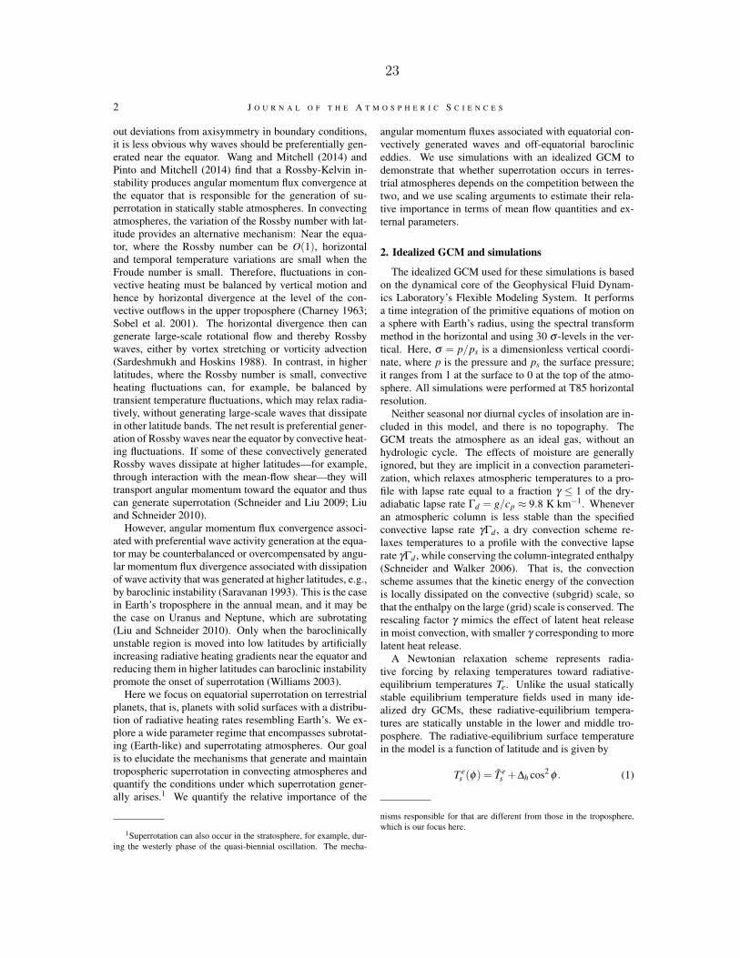
2 J O U R N A L O F T H E A T M O S P H E R I C S C I E N C E S

out deviations from axisymmetry in boundary conditions,it is less obvious why waves should be preferentially gen-erated near the equator. Wang and Mitchell (2014) andPinto and Mitchell (2014) find that a Rossby-Kelvin in-stability produces angular momentum flux convergence atthe equator that is responsible for the generation of su-perrotation in statically stable atmospheres. In convectingatmospheres, the variation of the Rossby number with lat-itude provides an alternative mechanism: Near the equa-tor, where the Rossby number can be O(1), horizontaland temporal temperature variations are small when theFroude number is small. Therefore, fluctuations in con-vective heating must be balanced by vertical motion andhence by horizontal divergence at the level of the con-vective outflows in the upper troposphere (Charney 1963;Sobel et al. 2001). The horizontal divergence then cangenerate large-scale rotational flow and thereby Rossbywaves, either by vortex stretching or vorticity advection(Sardeshmukh and Hoskins 1988). In contrast, in higherlatitudes, where the Rossby number is small, convectiveheating fluctuations can, for example, be balanced bytransient temperature fluctuations, which may relax radia-tively, without generating large-scale waves that dissipatein other latitude bands. The net result is preferential gener-ation of Rossby waves near the equator by convective heat-ing fluctuations. If some of these convectively generatedRossby waves dissipate at higher latitudes—for example,through interaction with the mean-flow shear—they willtransport angular momentum toward the equator and thuscan generate superrotation (Schneider and Liu 2009; Liuand Schneider 2010).

However, angular momentum flux convergence associ-ated with preferential wave activity generation at the equa-tor may be counterbalanced or overcompensated by angu-lar momentum flux divergence associated with dissipationof wave activity that was generated at higher latitudes, e.g.,by baroclinic instability (Saravanan 1993). This is the casein Earth’s troposphere in the annual mean, and it may bethe case on Uranus and Neptune, which are subrotating(Liu and Schneider 2010). Only when the baroclinicallyunstable region is moved into low latitudes by artificiallyincreasing radiative heating gradients near the equator andreducing them in higher latitudes can baroclinic instabilitypromote the onset of superrotation (Williams 2003).

Here we focus on equatorial superrotation on terrestrialplanets, that is, planets with solid surfaces with a distribu-tion of radiative heating rates resembling Earth’s. We ex-plore a wide parameter regime that encompasses subrotat-ing (Earth-like) and superrotating atmospheres. Our goalis to elucidate the mechanisms that generate and maintaintropospheric superrotation in convecting atmospheres andquantify the conditions under which superrotation gener-ally arises.1 We quantify the relative importance of the

1Superrotation can also occur in the stratosphere, for example, dur-ing the westerly phase of the quasi-biennial oscillation. The mecha-

angular momentum fluxes associated with equatorial con-vectively generated waves and off-equatorial barocliniceddies. We use simulations with an idealized GCM todemonstrate that whether superrotation occurs in terres-trial atmospheres depends on the competition between thetwo, and we use scaling arguments to estimate their rela-tive importance in terms of mean flow quantities and ex-ternal parameters.

2. Idealized GCM and simulations

The idealized GCM used for these simulations is basedon the dynamical core of the Geophysical Fluid Dynam-ics Laboratory’s Flexible Modeling System. It performsa time integration of the primitive equations of motion ona sphere with Earth’s radius, using the spectral transformmethod in the horizontal and using 30 σ -levels in the ver-tical. Here, σ = p/ps is a dimensionless vertical coordi-nate, where p is the pressure and ps the surface pressure;it ranges from 1 at the surface to 0 at the top of the atmo-sphere. All simulations were performed at T85 horizontalresolution.

Neither seasonal nor diurnal cycles of insolation are in-cluded in this model, and there is no topography. TheGCM treats the atmosphere as an ideal gas, without anhydrologic cycle. The effects of moisture are generallyignored, but they are implicit in a convection parameteri-zation, which relaxes atmospheric temperatures to a pro-file with lapse rate equal to a fraction γ ≤ 1 of the dry-adiabatic lapse rate Γd = g/cp ≈ 9.8 K km−1. Wheneveran atmospheric column is less stable than the specifiedconvective lapse rate γΓd , a dry convection scheme re-laxes temperatures to a profile with the convective lapserate γΓd , while conserving the column-integrated enthalpy(Schneider and Walker 2006). That is, the convectionscheme assumes that the kinetic energy of the convectionis locally dissipated on the convective (subgrid) scale, sothat the enthalpy on the large (grid) scale is conserved. Therescaling factor γ mimics the effect of latent heat releasein moist convection, with smaller γ corresponding to morelatent heat release.

A Newtonian relaxation scheme represents radia-tive forcing by relaxing temperatures toward radiative-equilibrium temperatures Te. Unlike the usual staticallystable equilibrium temperature fields used in many ide-alized dry GCMs, these radiative-equilibrium tempera-tures are statically unstable in the lower and middle tro-posphere. The radiative-equilibrium surface temperaturein the model is a function of latitude and is given by

T es (φ) = T e

s +∆h cos2 φ . (1)

nisms responsible for that are different from those in the troposphere,which is our focus here.

23

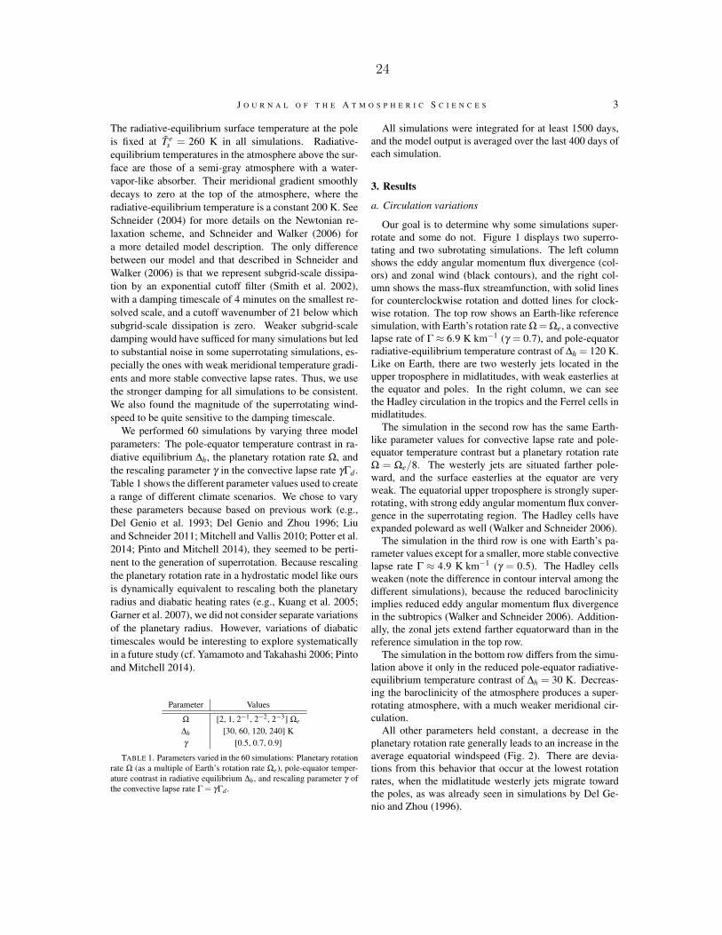
J O U R N A L O F T H E A T M O S P H E R I C S C I E N C E S 3

The radiative-equilibrium surface temperature at the poleis fixed at T e

s = 260 K in all simulations. Radiative-equilibrium temperatures in the atmosphere above the sur-face are those of a semi-gray atmosphere with a water-vapor-like absorber. Their meridional gradient smoothlydecays to zero at the top of the atmosphere, where theradiative-equilibrium temperature is a constant 200 K. SeeSchneider (2004) for more details on the Newtonian re-laxation scheme, and Schneider and Walker (2006) fora more detailed model description. The only differencebetween our model and that described in Schneider andWalker (2006) is that we represent subgrid-scale dissipa-tion by an exponential cutoff filter (Smith et al. 2002),with a damping timescale of 4 minutes on the smallest re-solved scale, and a cutoff wavenumber of 21 below whichsubgrid-scale dissipation is zero. Weaker subgrid-scaledamping would have sufficed for many simulations but ledto substantial noise in some superrotating simulations, es-pecially the ones with weak meridional temperature gradi-ents and more stable convective lapse rates. Thus, we usethe stronger damping for all simulations to be consistent.We also found the magnitude of the superrotating wind-speed to be quite sensitive to the damping timescale.

We performed 60 simulations by varying three modelparameters: The pole-equator temperature contrast in ra-diative equilibrium ∆h, the planetary rotation rate Ω, andthe rescaling parameter γ in the convective lapse rate γΓd .Table 1 shows the different parameter values used to createa range of different climate scenarios. We chose to varythese parameters because based on previous work (e.g.,Del Genio et al. 1993; Del Genio and Zhou 1996; Liuand Schneider 2011; Mitchell and Vallis 2010; Potter et al.2014; Pinto and Mitchell 2014), they seemed to be perti-nent to the generation of superrotation. Because rescalingthe planetary rotation rate in a hydrostatic model like oursis dynamically equivalent to rescaling both the planetaryradius and diabatic heating rates (e.g., Kuang et al. 2005;Garner et al. 2007), we did not consider separate variationsof the planetary radius. However, variations of diabatictimescales would be interesting to explore systematicallyin a future study (cf. Yamamoto and Takahashi 2006; Pintoand Mitchell 2014).

Parameter Values

Ω [2, 1, 2−1, 2−2, 2−3] Ωe

∆h [30, 60, 120, 240] Kγ [0.5, 0.7, 0.9]

TABLE 1. Parameters varied in the 60 simulations: Planetary rotationrate Ω (as a multiple of Earth’s rotation rate Ωe), pole-equator temper-ature contrast in radiative equilibrium ∆h, and rescaling parameter γ ofthe convective lapse rate Γ = γΓd .

All simulations were integrated for at least 1500 days,and the model output is averaged over the last 400 days ofeach simulation.

3. Results

a. Circulation variations

Our goal is to determine why some simulations super-rotate and some do not. Figure 1 displays two superro-tating and two subrotating simulations. The left columnshows the eddy angular momentum flux divergence (col-ors) and zonal wind (black contours), and the right col-umn shows the mass-flux streamfunction, with solid linesfor counterclockwise rotation and dotted lines for clock-wise rotation. The top row shows an Earth-like referencesimulation, with Earth’s rotation rate Ω=Ωe, a convectivelapse rate of Γ ≈ 6.9 K km−1 (γ = 0.7), and pole-equatorradiative-equilibrium temperature contrast of ∆h = 120 K.Like on Earth, there are two westerly jets located in theupper troposphere in midlatitudes, with weak easterlies atthe equator and poles. In the right column, we can seethe Hadley circulation in the tropics and the Ferrel cells inmidlatitudes.

The simulation in the second row has the same Earth-like parameter values for convective lapse rate and pole-equator temperature contrast but a planetary rotation rateΩ = Ωe/8. The westerly jets are situated farther pole-ward, and the surface easterlies at the equator are veryweak. The equatorial upper troposphere is strongly super-rotating, with strong eddy angular momentum flux conver-gence in the superrotating region. The Hadley cells haveexpanded poleward as well (Walker and Schneider 2006).

The simulation in the third row is one with Earth’s pa-rameter values except for a smaller, more stable convectivelapse rate Γ ≈ 4.9 K km−1 (γ = 0.5). The Hadley cellsweaken (note the difference in contour interval among thedifferent simulations), because the reduced baroclinicityimplies reduced eddy angular momentum flux divergencein the subtropics (Walker and Schneider 2006). Addition-ally, the zonal jets extend farther equatorward than in thereference simulation in the top row.

The simulation in the bottom row differs from the simu-lation above it only in the reduced pole-equator radiative-equilibrium temperature contrast of ∆h = 30 K. Decreas-ing the baroclinicity of the atmosphere produces a super-rotating atmosphere, with a much weaker meridional cir-culation.

All other parameters held constant, a decrease in theplanetary rotation rate generally leads to an increase in theaverage equatorial windspeed (Fig. 2). There are devia-tions from this behavior that occur at the lowest rotationrates, when the midlatitude westerly jets migrate towardthe poles, as was already seen in simulations by Del Ge-nio and Zhou (1996).

24

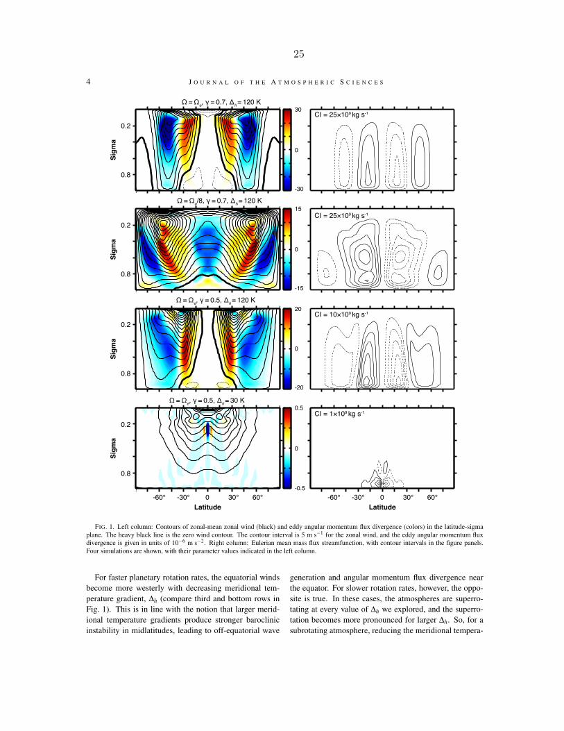
4 J O U R N A L O F T H E A T M O S P H E R I C S C I E N C E S

Sigm

a

!

!

0.2

0.8

Sigm

a

!

!

Sigm

a

!

!

Latitude

Sigm

a

!

!

Latitude

0.2

0.8

0.2

0.8

0.2

0.8

CI = 25×109 kg s-1

CI = 25×109 kg s-1

CI = 10×109 kg s-1

CI = 1×109 kg s-1

-60° -30° 0 30° 60° -60° -30° 0 30° 60°

Ω =Ωe, γ = 0.7, Δh = 120 K

Ω =Ωe/8, γ = 0.7, Δh = 120 K

Ω =Ωe, γ = 0.5, Δh = 120 K

Ω =Ωe, γ = 0.5, Δh = 30 K

0

30

-30

0

15

-15

0

20

-20

0

0.5

-0.5

FIG. 1. Left column: Contours of zonal-mean zonal wind (black) and eddy angular momentum flux divergence (colors) in the latitude-sigmaplane. The heavy black line is the zero wind contour. The contour interval is 5 m s−1 for the zonal wind, and the eddy angular momentum fluxdivergence is given in units of 10−6 m s−2. Right column: Eulerian mean mass flux streamfunction, with contour intervals in the figure panels.Four simulations are shown, with their parameter values indicated in the left column.

For faster planetary rotation rates, the equatorial windsbecome more westerly with decreasing meridional tem-perature gradient, ∆h (compare third and bottom rows inFig. 1). This is in line with the notion that larger merid-ional temperature gradients produce stronger baroclinicinstability in midlatitudes, leading to off-equatorial wave

generation and angular momentum flux divergence nearthe equator. For slower rotation rates, however, the oppo-site is true. In these cases, the atmospheres are superro-tating at every value of ∆h we explored, and the superro-tation becomes more pronounced for larger ∆h. So, for asubrotating atmosphere, reducing the meridional tempera-

25

J O U R N A L O F T H E A T M O S P H E R I C S C I E N C E S 5

Ω /Ωe

1/8 1/2 1 2

u(m

s-1)

-10

0

20

40Δh = 240 KΔh = 120 KΔh = 60 K

FIG. 2. Upper-tropospheric zonal wind at the equator versus Ω/Ωe withfixed values of ∆h and γ . For all three curves, γ = 0.7.

ture gradient can eventually lead to superrotation. On theother hand, decreasing the meridional temperature gradi-ent when the atmosphere is strongly superrotating (e.g.,for a slowly rotating planet) can weaken the superrotation.

b. Relation to wave activity sources

Why do some simulations superrotate while others donot? Quantifying the amount of equatorial eddy angu-lar momentum flux divergence and convergence owing toconvective and baroclinic sources provides insight. Asstated above, there must be a wave activity source at theequator that produces eddy angular momentum fluxes di-rected into the equatorial region in order to generate andsustain the angular momentum maximum there. Mak-ing the weak temperature gradient approximation near theequator, we write the vorticity equation neglecting thebaroclinic term, the twisting-tilting term, and friction:

∂ζa

∂ t+vΨ ·∇hζa ≈−ζa(∇h ·vχ)− (vχ ·∇hζa) = R. (2)

Here, ζa is the absolute vorticity, vχ + vΨ = v is the hor-izontal velocity decomposed into its rotational (Ψ) anddivergent (χ) components, and ∇h denotes the horizon-tal components of the del operator. Following Sardesh-mukh and Hoskins (1988) and Schneider and Liu (2009),we define the Rossby wave source as the fluctuating partof the right-hand side of this equation, R′ = R− R, withthe overbar denoting a zonal mean and primes deviationstherefrom.

The vorticity equation implies the approximate eddy en-strophy equation

12

∂ζ ′2

∂ t+ v′Ψζ ′∂yζa ≈ R′ζ ′, (3)

where vΨ is the rotational component of the meridional ve-locity v. Advection of eddy vorticity by the eddies them-selves (the triple correlation term) is neglected. In a statis-tically steady state and under the assumption that ζa 6= 0,the wave activity balance at the equator can then be writtenas (Andrews and Mcintyre 1976; Andrews and McIntyre1978; Edmon et al. 1980; Schneider and Liu 2009)

G =R′ζ ′

∂yζa= v′Ψζ ′ =− 1

cosφ∂y(u′Ψv′Ψ cos2 φ). (4)

The first equality defines G, the generation of wave activ-ity ζ ′2/(2∂yζa). Where G is positive, wave activity is gen-erated, and the eddy flux of angular momentum associatedwith the rotational flow converges; where G is negative,wave activity is dissipated, and the eddy flux of angularmomentum associated with the rotational flow diverges.Because the bulk of the eddy flux of angular momen-tum is associated with the rotational (geostrophic) flow,convergence/divergence of the eddy angular momentumflux u′Ψv′Ψ cosφ associated with the rotational flow is es-sentially synonymous with convergence/divergence of theoverall eddy angular momentum flux u′v′ cosφ .

We will use

〈G+e 〉=

1∆φ

∫ +5

−5

1∆σ

∫ σt

σt+∆σG+dσ dφ , (5)

the average of only the positive values G+ of G in theequatorial upper troposphere, as a measure of the waveactivity generation in the equatorial region, and hence asa measure of equatorially generated eddy angular momen-tum flux convergence, −(cos−1 φ)∂y(u′v′ cos2 φ)e. Herethe subscript e represents an average over the equatorial re-gion between −5 and +5. Angle brackets 〈·〉 representan average over a fixed depth in the upper troposphere,taken from the equatorial tropopause (defined using a crit-ical lapse rate of 2K/km) at the level σt = pt/ps to thelevel lying ∆σ = ∆p/ps = 0.3 below it. There is one sub-rotating simulation (Ω = 2Ωe,∆h = 120 K,γ = 0.7) withnegative values of 〈Ge〉 in the averaging region, such that〈G+

e 〉 is zero. We have omitted this simulation from thefigures that follow, because they show logarithms of 〈Ge〉,which is not a real number for this simulation.

Angular momentum divergence due to wave breakingof midlatitude baroclinic eddies can partially or fully com-pensate the angular momentum convergence in the equa-torial region associated with equatorial wave activity gen-eration 〈G+

e 〉. We want to quantify the angular momentumflux divergence M = (cos−1 φ)∂y(u′v′ cos2 φ)x (subscript

26

6 J O U R N A L O F T H E A T M O S P H E R I C S C I E N C E S

x for extratropical quantities) these baroclinic eddies gen-erate when they dissipate in the tropics. We use an upper-tropospheric average of the eddy angular momentum fluxdivergence M in the first “lobe” of divergence nearest tothe equator,

〈Md〉=1

∆φ

∫ φ1

φ2

1∆σ

∫ σt

σt+∆σMdσ dφ . (6)

After vertically averaging over the fixed depth in the up-per troposphere, we determine the latitudes bounding thefirst lobe of divergence for each simulation by starting atthe equator and finding the latitude φ1 where 〈M〉 becomespositive, indicating divergence, then continuing polewardup to the latitude φ2 where 〈M〉 changes sign to becomenegative. This average over the divergence lobe closest tothe equator is denoted by the subscript d. Divergence inthis region is produced when midlatitude baroclinic ed-dies dissipate there, for example, through filamentationand roll-up in their critical layers (Stewartson 1977; Ran-del and Held 1991), or through interaction with the mean-flow shear (Farrell 1987; Lindzen 1988; Huang and Robin-son 1998; O’Gorman and Schneider 2007; Ait-Chaalaland Schneider 2015). Thus, 〈Md〉 provides us with ameasure of wave activity dissipation associated with baro-clinic waves equatorward of their midlatitude generationregions. However, the measure is imperfect in that someangular momentum flux divergence associated with mid-latitude eddies in this region may be compensated by lo-cally generated angular momentum flux convergence, or itmay be augmented by divergence associated with equato-rial waves.

Figure 3 displays all 59 simulations as a function of〈G+

e 〉 and 〈Md〉. The black line is the one-to-one line. Thedifferent symbols indicate the planetary rotation rate foreach simulation, and the colors of the symbols indicatethe magnitude of the equatorial upper-tropospheric zonalwind. Positive values (red) indicate superrotation and neg-ative values (blue) subrotation.

The simulations that lie to the right of the one-to-oneline (i.e., with 〈G+

e 〉 > 〈Md〉) are generally superrotating,and those on the left (i.e., with 〈G+

e 〉< 〈Md〉) are generallysubrotating, with a couple of exceptions. That is, the ratioof the two parameters 〈G+

e 〉 and 〈Md〉 captures fairly wellwhether a given atmosphere is superrotating or not. It isclear that the planetary rotation rate plays a large role incontrolling 〈G+

e 〉: the slower rotation rates generally lieon the right side (superrotation), and the faster ones on theleft (subrotation).

There are two strongly superrotating simulations that lieon the left side of the line, and for which the scalings donot work well in the following figures. These simulationsboth have ∆h = 30K and γ = 0.5. They are the kind of sim-ulations for which we needed to increase the subgrid-scaledamping to decrease the noisiness of the simulations (sec-tion 2). We found that both the calculation of 〈G+

e 〉 and the

2Ωe

u (m s-1)

10-8 10-6 10-4

10-8

10-6

10-4

-20

0

20

40

ΩeΩe/2Ωe/4Ωe/4

〈G+e〉 (m s-2)

〈Md〉

(m s

-2)

FIG. 3. All simulations shown as a function of 〈G+e 〉 and 〈Md〉. In

this and subsequent figures, the marker color shows the mean zonalwind averaged within 5 degrees of the equator in the upper troposphere(in the same way that 〈G+

e 〉 is averaged). Positive values (red) indicatesuperrotation and negative values (blue) indicate subrotation. The dif-ferent symbols indicate the planetary rotation rates shown in the legend.The solid black line is the 1:1 line.

equatorial windspeed in these simulations with such lowbaroclinicity are very sensitive to the subgrid-scale damp-ing. For example, both simulations were more weakly su-perrotating in the upper troposphere with weaker damping.That subgrid-scale damping becomes dynamically impor-tant and leads to numerical sensitivities may explain whythese simulations are inconsistent with the theory.

4. Scaling theory

To understand more completely under which conditionssuperrotation arises, we develop a scaling theory for thewave activity generation 〈G+

e 〉 near the equator and for theoff-equatorial eddy angular momentum flux divergence〈Md〉.

a. Equatorial wave activity generation

To determine how 〈G+e 〉 scales with mean-flow param-

eters, we need scalings for R′, ζ ′, and ∂yζa. Becausethe Rossby wave source is R′ = R− R by definition, withR = ∇h · (ζavχ) according to Eq. (2), one can expand

R′ ≈ ∇h ·(

ζ ′vχ + ζav′χ)

≈(vχ ·∇h

)ζ ′+ζ ′

(∇h · vχ

)+(

v′χ ·∇h

)ζa + ζa

(∇h ·v′χ

),

(7)

27

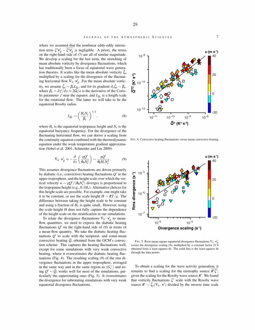
J O U R N A L O F T H E A T M O S P H E R I C S C I E N C E S 7

where we assumed that the nonlinear eddy-eddy interac-tion term ζ ′v′χ − ζ ′v′χ is negligible. A priori, the termson the right-hand side of (7) are all of similar magnitude.We develop a scaling for the last term, the stretching ofmean absolute vorticity by divergence fluctuations, whichhas traditionally been a focus of equatorial wave genera-tion theories. It scales like the mean absolute vorticity ζamultiplied by a scaling for the divergence of the fluctuat-ing horizontal flow ∇h ·v′χ . For the mean absolute vortic-ity, we assume ζa ∼ βeLβe , and for its gradient ∂yζa ∼ βe,where βe = ∂ f/∂y≈ 2Ω/a is the derivative of the Corio-lis parameter f near the equator, and Lβe is a length scalefor the rotational flow. The latter we will take to be theequatorial Rossby radius

Lβe ∼(

HeNe

βe

)1/2

, (8)

where He is the equatorial tropopause height and Ne is theequatorial buoyancy frequency. For the divergence of thefluctuating horizontal flow, we can derive a scaling fromthe continuity equation combined with the thermodynamicequation under the weak temperature gradient approxima-tion (Sobel et al. 2001; Schneider and Liu 2009)

∇h ·v′χ ≈−∂∂ z

(gQ′

θ0N2e

)∼ gQ′

θ0HeN2e. (9)

This assumes divergence fluctuations are driven primarilyby diabatic (i.e., convective) heating fluctuations Q′ in theupper troposphere, and the height scale over which the ver-tical velocity w ∼ gQ′/(θ0N2

e ) diverges is proportional tothe tropopause height (e.g., 0.1He). Alternative choices forthis height scale are possible. For example, one might takeit to be constant, or use the scale height H = RT/g. Thedifference between taking the height scale to be constantand using a fraction of He is quite small. However, usingthe scale height H does not fully capture the dependenceof the height scale on the stratification in our simulations.

To relate the divergence fluctuations ∇h · v′χ to mean-flow quantities, we need to express the diabatic heatingfluctuations Q′ on the right-hand side of (9) in terms ofa mean-flow quantity. We take the diabatic heating fluc-tuations Q′ to scale with the temporal- and zonal-meanconvective heating Q, obtained from the GCM’s convec-tion scheme. This captures the heating fluctuations well,except for some simulations with very weak convectiveheating, where it overestimates the diabatic heating fluc-tuations (Fig. 4). The resulting scaling (9) of the rms di-vergence fluctuations in the upper troposphere, averagedin the same way and in the same region as 〈G+

e 〉 and us-ing Q′ ∼ Q, works well for most of the simulations, par-ticularly the superrotating ones (Fig. 5). It overestimatesthe divergence for subrotating simulations with very weakequatorial divergence fluctuations.

10-11 10-10 10-9 10-8

10-12

10-10

10-8

-20

0

20

40u (m s-1)

Q 2 (K2 s-2)

Qʹ2

(K2 s

-2)

FIG. 4. Convective heating fluctuations versus mean convective heating.

10-6 10-5

10-7

10-6

10-5

-20

0

20

40u (m s-1)

Rm

s di

verg

ence

(s-1)

Divergence scaling (s-1)

FIG. 5. Root-mean-square equatorial divergence fluctuations ∇h ·v′χversus the divergence scaling (9), multiplied by a constant factor 21.9obtained from a least-squares fit. The solid line is the least-squares fitthrough the data points.

To obtain a scaling for the wave activity generation, itremains to find a scaling for the enstrophy source R′ζ ′,given the scaling for the Rossby wave source R′. We foundthat vorticity fluctuations ζ ′ scale with the Rossby wavesource R′ ∼ ζa(∇h · v′) divided by the inverse time scale

28

8 J O U R N A L O F T H E A T M O S P H E R I C S C I E N C E S

Ω -3/2

10-1 100

10-11

10-10

10-9

10-8

-20

0

20

40u (m s-1)

Ω /Ωe

Qʹ2

(K2 s

-2)

FIG. 6. Variance of convective heating fluctuations Q′ versus plane-tary rotation rate Ω for five series of simulations holding ∆h and γ con-stant and varying the rotation rate (each series is connected by a blackline).

given by the mean vorticity, ζa ∼ βeLβe . When combin-ing the scalings for R′ and ζ ′, one obtains ζ ′ ∼ ∇h · v′ ∼gQ/(θ0HeN2

e ). That is, vorticity fluctuations scale withdivergence fluctuations, as might be expected in regimeswhere the Rossby number is O(1). This implies that theother terms in Eq. (7) scale similarly to the stretching termon which we focused. The similarity of divergence andvorticity fluctuations also seems to imply that ζ ′ is notdependent on the planetary rotation rate; however, thisis not the case. The planetary rotation rate enters the ζ ′

scaling through the heating rate Q′, which decreases withincreasing rotation rate, empirically like Q′ ∼ Ω−3/4 be-tween Ω = Ωe and Ωe/4 (Fig. 6) in these simulations. Forthe highest and lowest rotation rates, the dependence ofQ′ on rotation rate becomes weaker. In general, Fig. 6shows that simulations with lower planetary rotation rateshave stronger mean equatorial heating rates and convectiveheating rate fluctuations—as is to be expected given thatlower planetary rotation rates necessitate weaker tempera-ture gradients and hence stronger mean meridional circu-lations to transport heat near the equator (Held and Hou1980). Correspondingly, divergence and vorticity fluctu-ations generally strengthen as the rotation rate decreases.

10-6 10-4

10-8

10-6

10-4

-20

0

20

40u (m s-1)

〈G+ e〉

(m s

-2)

〈G+e〉 scaling (m s-2)

FIG. 7. Equatorial wave activity source 〈G+e 〉 versus the scaling (10),

multiplied by a constant factor 89.3 obtained from a least-squares fit.The solid line is the least-squares fit through the data points.

Putting this all together we have a scaling for the equa-torial wave activity source 〈G+

e 〉:⟨G+

e⟩∼ Lβe(∇h ·v′)2

∼ g2Q2

θ 20 H3/2

e N7/2e β 1/2

e

.(10)

Figure 7 shows 〈G+e 〉 versus the scaling (10), with the

right-hand side multiplied by a factor 89.3, obtained froma least-squares fit. This factor is quite large because wehave suppressed an explicit small factor multiplying thetropopause height He in the height scale (e.g., 0.1He) ofvertical velocity divergence in Eq. (9), which would enterthe scaling (10) as an inverse square (e.g., as 0.1−2). Gen-erally, the scaling captures the variations of the wave ac-tivity source over ∼3 orders of magnitude quite well. Themost significant departures from a one-to-one relation-ship occur for subrotating simulations with weak pole-to-equator temperature gradients, for which the scaling over-estimates 〈G+

e 〉, in similar ways as the divergence scal-ing (9) overestimates actual divergence fluctuations (cf.Fig. 5).

b. Baroclinic angular momentum flux divergence

The baroclinic angular momentum fluxes originating inthe extratropics strengthen with increasing baroclinicity,for example, increasing pole-to-equator temperature con-trasts or decreasing static stability. Schneider and Walker

29

J O U R N A L O F T H E A T M O S P H E R I C S C I E N C E S 9

(2008) showed that in simulations of dry atmospheres sim-ilar to ours, the eddy angular momentum flux divergencescales with the mean available potential energy (MAPE)per unit mass in the troposphere and inversely with thewidth Lbc of the baroclinic zone over which MAPE is cal-culated:

〈Md〉 ∼MAPE

Lbc. (11)

Here, MAPE per unit mass is approximately

MAPE≈ g2

24N2x

(∆θθ0

)2

, (12)

where ∆θ is the meridional potential temperature con-trast across a baroclinic zone, θ0 is a reference value ofnear-surface potential temperature, and Nx is the extrat-ropical buoyancy frequency (Schneider 1981; Schneiderand Walker 2008). For simplicity we have omitted the de-pendence of MAPE on the supercriticality Sc, which wasdiscussed by Schneider and Walker (2008). Including itchanges the scaling only marginally for the simulations weconsider here. The width of the baroclinic zone only variesby a factor of two in our simulations, because the width ofthis zone is limited by the size of the planet for simulationswith low planetary rotation rate like the ones studied here.Hence, here we use a constant length scale Lbc = πa/4, butfor faster rotation rates it would need to be reduced, for ex-ample, like the Rossby radius, Lbc ∼ LR ∼Ω−1. Combin-ing these estimates and omitting nondimensional factorsgives

〈Md〉 ∼g2

LbcN2x

(∆θθ0

)2

. (13)

This scaling captures the dependence of the barocliniceddy angular momentum flux divergence in most simu-lations reasonably well, except in some very weakly baro-clinic simulations, in which it overestimates 〈Md〉 (Fig. 8).A least-squares fit suggests the right-hand side needs tobe multiplied by 0.174 to give a good fit to the simulationresults.

Combing the estimate for the equatorial wave activ-ity generation (angular momentum flux convergence) withthat for the baroclinic angular momentum flux divergence,we can introduce a nondimensional number

Sr =〈G+

e 〉〈Md〉

∼ αLbcN2

x

(H3e N3

e βe)1/2

(Q

Ne∆θ

)2

.

(14)

The factor α ≈ 500 is the ratio of the nondimensional fac-tors in the scalings for 〈G+

e 〉 and 〈Md〉. (Again, this fac-tor α is large primarily because we suppressed an explicitsmall factor multiplying the tropopause height He in thein the height scale of vertical velocity divergence.) The

10-6 10-5

10-8

10-6

10-4

-20

0

20

40

〈Md〉

(m s

-2)

〈Md〉 scaling (m s-2)

u (m s-1)

FIG. 8. Eddy angular momentum flux divergence 〈Md〉 versus thescaling (13), multiplied by a constant factor 0.174 obtained from a least-squares fit. The solid line is the least-squares fit through the data points.

nondimensional quantity Sr quantifies an atmosphere’spropensity for superrotation in terms of mean-flow quan-tities. When Sr & 1, an atmosphere will usually super-rotate, and when Sr . 1 it will usually subrotate. It tellsus that atmospheric superrotation is favored for strongerconvective heating at the equator (Q), reduced meridionaltemperature gradients (∆θ ), lower planetary rotation rates(βe ∼ Ω), and weaker equatorial (Ne) or stronger extrat-ropical (Nx) static stability. Because the convective heat-ing generally strengthens with decreasing rotation rate, thedependence of Sr on Ω is stronger than that occurring ex-plicitly through the β−1/2

e term.

5. Discussion

a. Mechanisms and origin of parameter dependences

Although idealized, the simulations performed herehave the basic ingredients to produce superrotation in ter-restrial atmospheres. The most important quantities con-trolling whether superrotation occurs or not in our simu-lations are the planetary rotation rate and the meridionaltemperature gradient, with, for example, the static stabil-ity in the tropics and extratropics playing secondary roles.

The dependence of Sr on rotation rate comes primarilyfrom the equatorial wave activity generation 〈G+

e 〉. Theextratropical 〈Md〉 will depend on rotation rate for fasterrotation rates (〈Md〉 ∼ Ω) because the width of the baro-clinic zone Lbc depends on rotation rate like the Rossbyradius, LR ∼ Ω−1. For the simulations discussed here,

30

10 J O U R N A L O F T H E A T M O S P H E R I C S C I E N C E S

however, the planetary scale limits this rotation rate depen-dence. The equatorial 〈G+

e 〉 ∼ Lβe(∇h ·v′)2 decreases withrotation rate for two primary reasons: The mean-squaredivergence (∇h · v′χ)2 ∼ Q2 depends on rotation rate be-cause the squared diabatic heating rate does, roughly like∼ Ω−3/2 in our simulations. Additionally, the equatorialRossby radius depends on rotation rate, Lβe ∼Ω−1/2.

Thus, for faster rotation rates, the baroclinic eddy an-gular momentum flux divergence increases with rotationrate because eddies get smaller and the angular momentumfluxes become more concentrated in narrower barocliniczones. Increases in meridional temperature contrasts be-cause of reduced efficiency of poleward energy transportcounteract some of this increase in baroclinic eddy an-gular momentum flux divergence (Schneider and Walker2008). By contrast, the equatorial wave activity generationdecreases with rotation rate both because the equatorialRossby radius increases and the convective heating fluctu-ations and divergence fluctuations weaken. For our simu-lations, the equatorial wave activity generation effect dom-inates and leads to Sr ∼Ω−2, that is, a strongly increasingpropensity for superrotation with decreasing rotation rate.(For faster rotation rates, this amplifies to Sr ∼Ω−3 whenadditionally the shrinking width of the baroclinic zone istaken into account.) This may account for the fact thatslowly rotating terrestrial atmospheres (e.g., Venus’) tendto exhibit superrotation.

The dependence of Sr on the meridional temperaturecontrast ∆θ enters explicitly only through the scalingfor 〈Md〉, which depends on MAPE ∼ (∆θ)2, yieldingSr ∼ (∆θ)−2. Thus, when meridional temperature gradi-ents are weak, there is less angular momentum flux diver-gence near the equator by midlatitude baroclinic eddies,and the propensity for superrotation increases. It is worth-while noting that when ∆θ is decreased in our simulations,the polar temperature remains constant and the equatorialand globally-averaged temperature decrease, decreasingthe equatorial tropopause height He (Thuburn and Craig2000; Schneider 2004) and adding to the propensity forsuperrotation. The meridional temperature contrast andthe rotation rate may also both affect the static stability inthe extratropics and near the equator, which in themselveshave opposing effects on Sr ∼ N2

x N−7/2e .

To look at the equatorial wave structure more closely,Fig. 9 shows the correlation coefficient between equatorialdivergence fluctuations at a reference point and horizon-tal streamfunction fluctuations at 300 hPa for a superrotat-ing simulation with slow planetary rotation (Ω = Ωe/8,∆h = 120 K, γ = 0.7; see second row of Fig. 1). Thereference point is indicated by a black dot at the equa-tor at 180 longitude. The correlation coefficients be-tween divergence fluctuations at the equator and, on theone hand, horizontal streamfunction fluctuations (colors)and, on the other hand, wind fluctuations (arrows), indi-cate a Rossby (rotational) wave structure (Matsuno 1966).

°

°

°

°

°

Latitude

° ° °Longitude

FIG. 9. Correlation coefficient (colors) between divergence fluctu-ations at a reference point on the equator (black dot) and horizontalstreamfunction fluctuations at 300 hPa, for the superrotating simulationwith Ω = Ωe/8, ∆h = 120 K, and γ = 0.7 (see second row of Fig. 1).Arrows represent correlation coefficients between wind fluctuations anddivergence fluctuations at the equator. An arrow pointing right corre-sponds to a positive correlation for u′ and zero correlation for v′; anarrow pointing upward corresponds to a positive correlation of for v′

and zero for u′. The lengths of the arrows indicate the magnitude of thecorrelations.

The Rossby wave has zonal velocities symmetric aboutthe equator and meridional velocities antisymmetric aboutthe equator. The equatorial Rossby radius, which deter-mines the decay of meridional velocity correlations awayfrom the equator, appears to extend over much of a hemi-sphere, consistent with the low rotation rate in this simu-lation (Ω = Ωe/8). The correlations between wind fluctu-ations and divergence fluctuations at the equator (arrows)indicate angular momentum transport toward the equator.They also show that no more than the usual tilt of phaselines with latitude is needed to generate the angular mo-mentum transport; it is not necessary to see outright merid-ional propagation of wave packets for angular momentumtransport to occur. This overall picture is consistent withour theoretical considerations, which assign primary im-portance to equatorial Rossby waves and their equator-ward angular momentum transport in the generation of su-perrotation.

Figure 10 shows the eddy angular momentum fluxcospectra (black contours for positive and blue contoursfor negative fluxes) versus latitude at the level σ = 0.3 fora subrotating and a superrotating simulation (correspond-ing to the first and second rows of Fig. 1). The thick blackline is the mean zonal wind at the same level. The sub-rotating simulation shows similar features to what we seeon Earth (Randel and Held 1991): baroclinic eddies gen-erated in midlatitudes have phase speeds of O(10 m s−1)and dissipate near their critical latitudes, which producesconvergence of eddy angular momentum fluxes in midlat-itudes and divergence primarily on the equatorward flanks

31

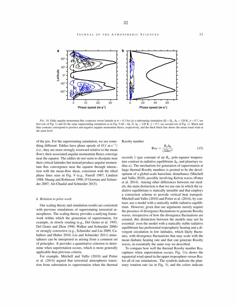
J O U R N A L O F T H E A T M O S P H E R I C S C I E N C E S 11

Phase speed (m s-1)0

Latit

ude

-60°

-30°

0°

30°

60°

Phase speed (m s-1)

a b

10 20 30 0 20 40 60

FIG. 10. Eddy angular momentum flux cospectra versus latitude at σ = 0.3 for (a) a subrotating simulation (Ω = Ωe, ∆h = 120 K, γ = 0.7, seefirst row of Fig. 1) and (b) the same superrotating simulation as in Fig. 9 (Ω = Ωe/8, ∆h = 120 K, γ = 0.7, see second row of Fig. 1). Black andblue contours correspond to positive and negative angular momentum fluxes, respectively, and the thick black line shows the mean zonal wind atthe same level.

of the jets. For the superrotating simulation, we see some-thing different: Eddies have phase speeds of O(1 m s−1)(i.e., they are more strongly westward relative to the meanflow); their associated angular momentum fluxes convergenear the equator. The eddies do not seem to dissipate neartheir critical latitudes but instead produce angular momen-tum flux convergence near the equator through interac-tion with the mean-flow shear, consistent with the tiltedphase lines seen in Fig. 9 (e.g., Farrell 1987; Lindzen1988; Huang and Robinson 1998; O’Gorman and Schnei-der 2007; Ait-Chaalal and Schneider 2015).

b. Relation to prior work

Our scaling theory and simulation results are consistentwith previous simulations of superrotating terrestrial at-mospheres. The scaling theory provides a unifying frame-work within which the generation of superrotation, forexample, in slowly rotating (e.g., Del Genio et al. 1993;Del Genio and Zhou 1996; Walker and Schneider 2006)or strongly convective (e.g., Schneider and Liu 2009; Ca-ballero and Huber 2010; Liu and Schneider 2011) atmo-spheres can be interpreted as arising from a common setof principles. It provides a quantitative criterion to deter-mine when superrotation occurs, which is more generallyapplicable than previous criteria.

For example, Mitchell and Vallis (2010) and Potteret al. (2014) argued that terrestrial atmospheres transi-tion from subrotation to superrotation when the thermal

Rossby number

RoT =Ra∆h

(2Ωa)2 (15)

exceeds 1 (gas constant of air Ra, pole-equator tempera-ture contrast in radiative equilibrium ∆h, and planetary ra-dius a). The mechanism for generation of superrotation atlarge thermal Rossby numbers is posited to be the devel-opment of a global-scale baroclinic disturbance (Mitchelland Vallis 2010), possibly involving Kelvin waves (Potteret al. 2014). Among other differences between our mod-els, the main distinction is that we use one in which the ra-diative equilibrium is statically unstable and that employsa convection scheme to provide vertical heat transport.Mitchell and Vallis (2010) and Potter et al. (2014), by con-trast, use a model with a statically stable radiative equilib-rium. However, given that our arguments merely requirethe presence of divergence fluctuations to generate Rossbywaves, irrespective of how the divergence fluctuations arecreated, this distinction between the models may not beessential: even the model with a statically stable radiativeequilibrium has preferential tropospheric heating and a di-vergent circulation in low latitudes, which likely fluctu-ates, with divergence fluctuations that may scale with themean diabatic heating rate and that can generate Rossbywaves, in essentially the same way we described.

To compare how well the thermal Rossby number RoTcaptures when superrotation occurs, Fig. 11a shows theequatorial wind speed in the upper troposphere versus RoTfor all of our simulations. The symbols indicate the plan-etary rotation rate (as in Fig. 3), and the colors indicate

32

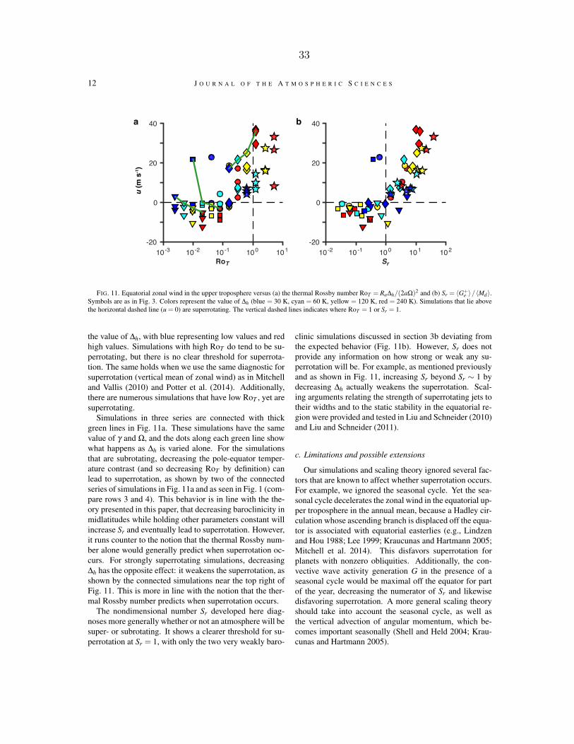
12 J O U R N A L O F T H E A T M O S P H E R I C S C I E N C E S

a

RoT

10-3 10-2 10-1 100 101

u (m

s-1)

-20

0

20

40 b

Sr

10-2 10-1 100 101 102-20

0

20

40

FIG. 11. Equatorial zonal wind in the upper troposphere versus (a) the thermal Rossby number RoT = Ra∆h/(2aΩ)2 and (b) Sr = 〈G+e 〉/〈Md〉.

Symbols are as in Fig. 3. Colors represent the value of ∆h (blue = 30 K, cyan = 60 K, yellow = 120 K, red = 240 K). Simulations that lie abovethe horizontal dashed line (u = 0) are superrotating. The vertical dashed lines indicates where RoT = 1 or Sr = 1.

the value of ∆h, with blue representing low values and redhigh values. Simulations with high RoT do tend to be su-perrotating, but there is no clear threshold for superrota-tion. The same holds when we use the same diagnostic forsuperrotation (vertical mean of zonal wind) as in Mitchelland Vallis (2010) and Potter et al. (2014). Additionally,there are numerous simulations that have low RoT , yet aresuperrotating.

Simulations in three series are connected with thickgreen lines in Fig. 11a. These simulations have the samevalue of γ and Ω, and the dots along each green line showwhat happens as ∆h is varied alone. For the simulationsthat are subrotating, decreasing the pole-equator temper-ature contrast (and so decreasing RoT by definition) canlead to superrotation, as shown by two of the connectedseries of simulations in Fig. 11a and as seen in Fig. 1 (com-pare rows 3 and 4). This behavior is in line with the the-ory presented in this paper, that decreasing baroclinicity inmidlatitudes while holding other parameters constant willincrease Sr and eventually lead to superrotation. However,it runs counter to the notion that the thermal Rossby num-ber alone would generally predict when superrotation oc-curs. For strongly superrotating simulations, decreasing∆h has the opposite effect: it weakens the superrotation, asshown by the connected simulations near the top right ofFig. 11. This is more in line with the notion that the ther-mal Rossby number predicts when superrotation occurs.

The nondimensional number Sr developed here diag-noses more generally whether or not an atmosphere will besuper- or subrotating. It shows a clearer threshold for su-perrotation at Sr = 1, with only the two very weakly baro-

clinic simulations discussed in section 3b deviating fromthe expected behavior (Fig. 11b). However, Sr does notprovide any information on how strong or weak any su-perrotation will be. For example, as mentioned previouslyand as shown in Fig. 11, increasing Sr beyond Sr ∼ 1 bydecreasing ∆h actually weakens the superrotation. Scal-ing arguments relating the strength of superrotating jets totheir widths and to the static stability in the equatorial re-gion were provided and tested in Liu and Schneider (2010)and Liu and Schneider (2011).

c. Limitations and possible extensions

Our simulations and scaling theory ignored several fac-tors that are known to affect whether superrotation occurs.For example, we ignored the seasonal cycle. Yet the sea-sonal cycle decelerates the zonal wind in the equatorial up-per troposphere in the annual mean, because a Hadley cir-culation whose ascending branch is displaced off the equa-tor is associated with equatorial easterlies (e.g., Lindzenand Hou 1988; Lee 1999; Kraucunas and Hartmann 2005;Mitchell et al. 2014). This disfavors superrotation forplanets with nonzero obliquities. Additionally, the con-vective wave activity generation G in the presence of aseasonal cycle would be maximal off the equator for partof the year, decreasing the numerator of Sr and likewisedisfavoring superrotation. A more general scaling theoryshould take into account the seasonal cycle, as well asthe vertical advection of angular momentum, which be-comes important seasonally (Shell and Held 2004; Krau-cunas and Hartmann 2005).

33

J O U R N A L O F T H E A T M O S P H E R I C S C I E N C E S 13

We also focused on transient sources of equatorialRossby waves at the expense of stationary sources, whichin several previous studies have been shown to be ableto generate superrotation if they are strong enough (e.g.,Suarez and Duffy 1992; Saravanan 1993; Joshi et al. 1997;Kraucunas and Hartmann 2005; Merlis and Schneider2010; Arnold et al. 2012; Pierrehumbert 2011). Our scal-ing theory can be extended to take stationary equatorialwave activity generation into account, by considering howthe stationary divergence perturbation and equatorial waveactivity generation scale with parameters controlling thestrength of the stationary wave source. In particular, itis to be expected that the importance of equatorial waveactivity generation owing to stationary heat sources in-creases in importance relative to baroclinic eddy angularmomentum flux divergence as the planetary rotation ratedecreases for the same reasons the importance of transientequatorial wave activity generation increases. Thus, weexpect that stationary heat sources (e.g., stellar heating fo-cused on a substellar point on tidally locked planets) moreeasily lead to equatorial superrotation on slowly rotatingplanets.

6. Conclusions

We have presented simulations and a scaling theory thatestablish conditions under which superrotation occurs interrestrial atmospheres. By varying the planetary rota-tion rate, the pole-equator temperature contrast in radia-tive equilibrium, and a scaling parameter for the convec-tive lapse rate, we generated a wide range of atmosphericflows, some superrotating and some subrotating.

The theory presented here is based on a simple ideagoing back to Saravanan (1993) about two competingsources for eddy angular momentum flux convergence atthe equator. The first is a source at the equator: Rossbywaves generated by convective heating fluctuations. Asthese waves dissipate away from the equator, they con-verge angular momentum into the equatorial region, in-creasing the propensity for superrotation. The other sourceis baroclinic instability in midlatitudes, which generatesRossby waves in midlatitudes that dissipate farther equa-torward, thus extracting momentum from lower latitudes.This mechanism decreases the propensity for superrota-tion. Quantifying the magnitude of the two mechanisms,introducing their nondimensional ratio Sr, and developinga scaling for it in terms of mean-flow quantities leads toour theory and sheds light on the conditions under whichsuperrotation occurs. Our simulation results and scalingtheory show that:

1. Superrotation occurs when the eddy angular mo-mentum flux convergence associated with equatorialwave activity generation exceeds eddy angular mo-mentum flux divergence near the equator producedby midlatitude baroclinic eddies (i.e., Sr & 1).

2. Superrotation is favored for low planetary rotationrates and/or strong diabatic heating.

3. Superrotation is favored when midlatitude baroclin-icity is weak.

Our simulations confirm that superrotation is preferredfor slowly rotating planets like Venus and Titan, a re-sult that was obtained by Del Genio et al. (1993) andDel Genio and Zhou (1996) in a similar set of simula-tions. The scaling arguments presented here help us under-stand why slowly rotating planets exhibit superrotation. Inour simulations, equatorial convective heating fluctuationsstrengthen with decreasing rotation rate, generating wavesthat transport momentum upgradient toward the equator,leading to superrotation. Such convective heating fluctu-ations may play a role on Venus, in the shallow convec-tive layers observed in the upper troposphere (Markiewiczet al. 2007). The equatorial wave activity generationstrengthens as the planetary rotation rate decreases primar-ily because the diabatic heating rate strengthens. Thus,similar arguments may also apply for other mechanismsthat increase the diabatic heating or more generally, diver-gence fluctuations at the equator. For example, stationaryor nearly stationary heat sources that generate equatorialRossby waves have been suggested to play a role on Venusnear the subsolar point (Gierasch et al. 1997).

Strengthening equatorial convective heating fluctua-tions may also explain why some Earth climate modelsexhibit a transition to superrotation under extreme globalwarming (e.g., Caballero and Huber 2010). In this sce-nario, convective heating at the equator strengthens due togreenhouse gas forcing, and meridional temperature gradi-ents decrease because of polar amplification of the warm-ing. Both factors favor superrotation.

Acknowledgments. Some of the scaling results in thispaper were presented at the 18th Conference on Atmo-spheric and Oceanic Fluid Dynamics in 2011. The re-search was supported by the U.S. National Science Foun-dation through Grant AGS-1049201 and a Graduate Re-search Fellowship.

ReferencesAit-Chaalal, F., and T. Schneider, 2015: Why eddy momentum fluxes

are concentrated in the upper troposphere. J. Atmos. Sci., 72, 1585–1604.

Andrews, D. G., and M. E. Mcintyre, 1976: Planetary waves in hori-zontal and vertical shear: the generalized Eliassen-Palm relation andthe mean zonal acceleration. J. Atmos. Sci., 33, 2031–2048.

Andrews, D. G., and M. E. McIntyre, 1978: An exact theory of nonlin-ear waves on a Lagrangian-mean flow. J. Fluid Mech., 89, 609–646.

Arnold, N. P., E. Tziperman, and B. Farrell, 2012: Abrupt transitionto strong superrotation driven by equatorial wave resonance in anidealized GCM. J. Atmos. Sci., 69, 626–640.

34

14 J O U R N A L O F T H E A T M O S P H E R I C S C I E N C E S

Caballero, R., and M. Huber, 2010: Spontaneous transition to superro-tation in warm climates simulated by CAM3. Geophys. Res. Lett.,37, doi:10.1029/2010GL043468.

Charney, J. G., 1963: A note on large-scale motions in the tropics. J.Atmos. Sci., 20, 607–609.

Del Genio, A. D., and W. Zhou, 1996: Simulations of superrotation onslowly rotating planets: Sensitivity to rotation and initial condition.Icarus, 120, 332–343.

Del Genio, A. D., W. Zhou, and T. P. Eichler, 1993: Equatorial superro-tation in a slowly rotating GCM: Implications for Titan and Venus.Icarus, 101, 1–17.

Edmon, H. J., Jr., B. J. Hoskins, and M. E. McIntyre, 1980: Eliassen-Palm cross sections for the troposphere. J. Atmos. Sci., 37, 2600–2616.

Farrell, B., 1987: Developing disturbances in shear. J. Atmos. Sci., 44,2191–2199.

Garner, S. T., D. M. W. Frierson, I. M. Held, O. Pauluis, and G. K. Val-lis, 2007: Resolving convection in a global hypohydrostatic model.J. Atmos. Sci., 64, 2061–2075.

Gierasch, P., and Coauthors, 1997: The general circulation of the Venusatmosphere: An assessment. Venus II: Geology, Geophysics, Atmo-sphere, and Solar Wind Environment, S. W. Bougher, D. M. Hunten,and R. J. Phillips, Eds., The University of Arizona Press, 459–500.

Held, I. M., 1975: Momentum transport by quasi-geostrophic eddies. J.Atmos. Sci., 32, 1494–1497.

Held, I. M., 1999: Equatorial superrotation in Earth-like atmosphericmodels, Bernhard Haurwitz Memorial Lecture, American Meteoro-logical Society. Available at www.gfdl.noaa.gov/˜ih.

Held, I. M., and A. Y. Hou, 1980: Nonlinear axially symmetric circula-tions in a nearly inviscid atmosphere. J. Atmos. Sci., 37, 515–533.

Hide, R., 1969: Dynamics of the atmospheres of the major planets withan appendix on the viscous boundary layer at the rigid bounding sur-face of an electrically-conducting rotating fluid in the presence of amagnetic field. J. Atmos. Sci., 26, 841–853.

Huang, H.-P., and W. A. Robinson, 1998: Two-dimensional turbulenceand persistent zonal jets in a global barotropic model. J. Atmos. Sci.,55, 611–632.

Joshi, M., R. Haberle, and R. Reynolds, 1997: Simulations of the at-mospheres of synchronously rotating terrestrial planets orbiting Mdwarfs: conditions for atmospheric collapse and the implications forhabitability. Icarus, 129, 450–465.

Kostiuk, T., K. E. Fast, T. A. Livengood, T. Hewagama, J. J. Goldstein,F. Espenak, and D. Buhl, 2001: Direct measurement of winds onTitan. Geophys. Res. Lett., 28, 2361–2364.

Kraucunas, I., and D. L. Hartmann, 2005: Equatorial superrotation andthe factors controlling the zonal-mean zonal winds in the tropicalupper troposphere. J. Atmos. Sci., 62, 371–389.

Kuang, Z., P. N. Blossey, and C. S. Bretherton, 2005: A new ap-proach for 3D cloud-resolving simulations of large-scale atmo-spheric circulation. Geophys. Res. Lett., 32, L02 809, doi:10.1029/2004GL021024.

Lee, S., 1999: Why are the climatological zonal winds easterly in theequatorial upper troposphere? J. Atmos. Sci., 56, 1353–1363.

Lindzen, R. S., 1988: Instability of plane parallel shear flow (towarda mechanistic picture of how it works). Pure Appl. Geophys., 126,103–121.

Lindzen, R. S., and A. Y. Hou, 1988: Hadley circulations for zonallyaveraged heating centered off the equator. J. Atmos. Sci., 45, 2416–2427.

Liu, J., and T. Schneider, 2010: Mechanisms of jet formation onthe giant planets. J. Atmos. Sci., 67, 3652–3672, doi:10.1175/2010JAS3492.1.

Liu, J., and T. Schneider, 2011: Convective generation of equatorial su-perrotation in planetary atmospheres. J. Atmos. Sci., 68, 2742–2756,doi:10.1175/JAS-D-10-05013.1.

Markiewicz, W. J., and Coauthors, 2007: Morphology and dynamics ofthe upper cloud layer of Venus. Nature, 450, 633–636.

Matsuno, T., 1966: Quasi-geostrophic motions in the equatorial area. J.Meteor. Soc. Japan, 44, 25–42.

Merlis, T. M., and T. Schneider, 2010: Atmospheric dynamics of Earth-like tidally locked aquaplanets. J. Adv. Mod. Earth Sys., 2, 13, doi:10.3894/JAMES.2010.2.13.

Mitchell, J. L., and G. K. Vallis, 2010: The transition to superrotationin terrestrial atmospheres. J. Geophys. Res., 115, E12 008, doi:10.1029/2010JE003587.

Mitchell, J. L., G. K. Vallis, and S. F. Potter, 2014: Effects of the sea-sonal cycle on superrotation in planetary atmospheres. Astrophys. J.,787, 23, doi:10.1088/0004-637X/787/1/23.

O’Gorman, P. A., and T. Schneider, 2007: Recovery of atmosphericflow statistics in a general circulation model without nonlinear eddy–eddy interactions. Geophys. Res. Lett., 34, L22 801.

Pierrehumbert, R. T., 2011: A palette of climates for Gliese 581g. As-trophys. J. Lett., 726, L8.

Pinto, J. R. D., and J. L. Mitchell, 2014: Atmospheric superrotationin an idealized GCM: Parameter dependence of the eddy response.Icarus, 238, 93–109.

Porco, C. C., and Coauthors, 2003: Cassini imaging of Jupiter’s atmo-sphere, satellites, and rings. Science, 299, 1541–1547.

Potter, S. F., G. K. Vallis, and J. L. Mitchell, 2014: Spontaneous super-rotation and the role of Kelvin waves in an idealized dry GCM. J.Atmos. Sci., 71, 596–614.

Randel, W. J., and I. M. Held, 1991: Phase speed spectra of transienteddy fluxes and critical layer absorption. J. Atmos. Sci., 48, 688–697.

Sanchez-Lavega, A., R. Hueso, and S. Perez-Hoyos, 2007: The three-dimensional structure of Saturn’s equatorial jet at cloud level. Icarus,187, 510–519.

Saravanan, R., 1993: Equatorial superrotation and maintenance of thegeneral circulation in two-level models. J. Atmos. Sci., 50, 1211–1227.

Sardeshmukh, P. D., and B. J. Hoskins, 1988: The generation of globalrotational flow by steady idealized tropical divergence. J. Atmos. Sci.,7, 1228–1251.

Schneider, E. K., 1981: On the amplitudes reached by baroclinicallyunstable disturbances. J. Atmos. Sci., 38, 2142–2149.

35

J O U R N A L O F T H E A T M O S P H E R I C S C I E N C E S 15

Schneider, T., 2004: The tropopause and the thermal stratification inthe extratropics of a dry atmosphere. J. Atmos. Sci., 61, 1317–1340,doi:10.1175/1520-0469(2004)061〈1317:TTATTS〉2.0.CO;2.

Schneider, T., 2006: The General Circulation of the Atmosphere. An-nual Review of Earth and Planetary Sciences, 34, 655–688, doi:10.1146/annurev.earth.34.031405.125144.

Schneider, T., and J. Liu, 2009: Formation of jets and equatorial su-perrotation on Jupiter. J. Atmos. Sci., 66, 579–601, doi:10.1175/2008JAS2798.1.

Schneider, T., and C. C. Walker, 2006: Self-organization of atmosphericmacroturbulence into critical states of weak nonlinear eddy–eddy in-teractions. J. Atmos. Sci., 63, 1569–1586, doi:10.1175/JAS3699.1.

Schneider, T., and C. C. Walker, 2008: Scaling laws and regime tran-sitions of macroturbulence in dry atmospheres. J. Atmos. Sci., 65,2153–2173, doi:10.1175/2007JAS2616.1.

Schubert, G., 1983: General circulation and the dynamical state of theVenus atmosphere. Venus, 1, 681–765.

Shell, K. M., and I. M. Held, 2004: Abrupt transition to strong superro-tation in an axisymmetric model of the upper troposphere. J. Atmos.Sci., 61 (23), 2928–2935.

Smith, K., G. Boccaletti, C. Henning, I. Marinov, C. Tam, I. Held, andG. Vallis, 2002: Turbulent diffusion in the geostrophic inverse cas-cade. J. Fluid Mech., 469, 13–48.

Sobel, A. H., J. Nilsson, and L. M. Polvani, 2001: The weak temper-ature gradient approximation and balanced tropical moisture waves.J. Atmos. Sci., 58, 3650–3665.

Stewartson, K., 1977: The evolution of the critical layer of a Rossbywave. Geophys. Astrophys. Fluid Dyn., 9, 185–200.

Suarez, M. J., and D. G. Duffy, 1992: Terrestrial superrotation: A bifur-cation of the general circulation. J. Atmos. Sci., 49, 1541–1554.

Thuburn, J., and G. C. Craig, 2000: Stratospheric influence ontropopause height: The radiative constraint. J. Atmos. Sci., 57, 17–28.

Walker, C. C., and T. Schneider, 2006: Eddy influences on hadley circu-lations: Simulations with an idealized gcm. J. Atmos. Sci., 63, 3333–3350, doi:10.1175/JAS3821.1.

Wang, P., and J. L. Mitchell, 2014: Planetary ageostrophic instabilityleads to superrotation. Geophys. Res. Lett., 41 (12), 4118–4126.

Williams, G. P., 2003: Barotropic instability and equatorial superrota-tion. J. Atmos. Sci., 60 (17), 2136–2152.

Yamamoto, M., and M. Takahashi, 2006: Superrotation maintained bymeridional circulation and waves in a Venus-like AGCM. J. Atmos.Sci., 63, 3296–3314, doi:10.1175/JAS3859.1.

36

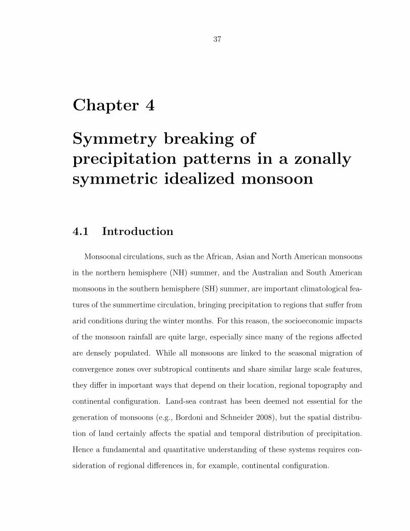
37

Chapter 4

Symmetry breaking ofprecipitation patterns in a zonallysymmetric idealized monsoon

4.1 Introduction

Monsoonal circulations, such as the African, Asian and North American monsoons

in the northern hemisphere (NH) summer, and the Australian and South American

monsoons in the southern hemisphere (SH) summer, are important climatological fea-

tures of the summertime circulation, bringing precipitation to regions that suffer from

arid conditions during the winter months. For this reason, the socioeconomic impacts

of the monsoon rainfall are quite large, especially since many of the regions affected

are densely populated. While all monsoons are linked to the seasonal migration of

convergence zones over subtropical continents and share similar large scale features,

they differ in important ways that depend on their location, regional topography and

continental configuration. Land-sea contrast has been deemed not essential for the

generation of monsoons (e.g., Bordoni and Schneider 2008), but the spatial distribu-

tion of land certainly affects the spatial and temporal distribution of precipitation.

Hence a fundamental and quantitative understanding of these systems requires con-

sideration of regional differences in, for example, continental configuration.

38

Monsoons are characterized by alternating wet and dry seasons and seasonally

reversing winds. Because of this they have been described as planetary-scale sea

breezes (Webster and Fasullo 2003), where pressure gradients arising from differential

heating of land and ocean drive the monsoonal overturning circulation. In the work of

Bordoni and Schneider (2008), the low thermal inertia of the land surface compared

with that of the ocean, and not differential heating, is argued to be important for

the development of monsoons. Monsoon transitions occur in their model even in the

absence of any surface inhomogeneity when the zonal momentum budget in the upper

branch of the winter Hadley cell transitions from a regime in which eddy momentum

fluxes play a dominant role to a regime in which they are less dominant, allowing

the circulation to approach the angular momentum-conserving limit. The transition

between the two different regimes is made rapid by eddy-mean flow feedbacks that

can act on seasonal time scales only if the lower-level temperatures can adjust rapidly,

hence only if the thermal inertia of the lower boundary is sufficiently small. These

arguments, which hold for a statistically zonally and hemispherically symmetric cli-

mate, might also be relevant for the seasonal onset of the Indian monsoon, in which

land in the longitudinal sector over which the monsoon develops is primarily confined

to the NH. Our experimental design is modeled after the Indian monsoon sector, and

our goal is to understand how adding a zonally symmetric continent in the NH affects

the resulting monsoonal circulation.

For decades, axisymmetric models have been used to study tropical overturning

circulations, such as Hadley and monsoonal circulations, in steady state (e.g., Held

and Hou 1980; Lindzen and Hou 1988; Plumb and Hou 1992; Prive and Plumb 2007a).

Held and Hou (1980) explained the existence of the annual-mean Hadley circulation

using angular momentum conservation. Lindzen and Hou (1988) expanded upon Held

and Hou (1980) by exploring the response to an off-equatorial peak in the forcing,

and were able to replicate a “winter” cell, seen in observations. Plumb and Hou

39

(1992) studied the response of the atmospheric circulation to a localized subtropical

temperature perturbation, which is more relevant to monsoonal circulations. They

showed that the onset of a cross-equatorial monsoonal circulation only occurs for a

supercritical forcing, and they argued that this threshold behavior could be relevant

for the rapid seasonal monsoon onset. Prive and Plumb (2007a) used an axisymmetric

model to develop a theory for the location of the poleward extent of the monsoon,

and found that the poleward limit coincides with the maximum of the sub-cloud

moist static energy (MSE), which is in agreement with the quasi-equilibrium view

of monsoons (Emanuel 1995). These axisymmetric studies are fundamental papers

in the tropical dynamics literature, because they attempt to understand the global

circulation using concepts of angular momentum and energy conservation. Although

highly idealized, and therefore arguably not very realistic, these models have provided

theoretical insight into the basic workings of the monsoon, as well as the Hadley cell.

The simulations presented in this work are performed with a three-dimensional

idealized general circulation model (GCM) that includes a seasonal cycle. Unlike

axisymmetric models, this model resolves large-scale eddies, which in the extratropics

effect energy and momentum transport. The extratropical eddies have been shown

to play an important role in the annually-averaged tropical Hadley cell (Walker and

Schneider 2006; Schneider 2006) and in the seasonal transition of the monsoonal

circulation (Bordoni and Schneider 2008). Three-dimensional models of intermediate

complexity have been used before to study the mechanisms that drive monsoons. For

example, Chou et al. (2001) found that “ventilation” (negative advection of MSE

from the ocean over the continent) plays a large role in setting the poleward extent of

the monsoonal precipitation over a zonally-asymmetric continent. Prive and Plumb

(2007b) found that lower-level eddies associated with the monsoonal flow redistribute

the MSE such that the maximum is closer to the equator than in the axisymmetric

models. These studies are in agreement with the theory that the circulation boundary

40

is co-located with the maximum sub-cloud MSE. Alternatively, Shaw (2014) found

that the NH winter cell circulation boundary is located at the latitude of maximum

planetary-scale “waviness” in reanalysis data. She verified this with an aquaplanet

GCM with stationary subtropical forcing.

Recent work has focused on determining what sets the position of the intertropical

convergence zone, or ITCZ, in the annual mean (e.g., Frierson et al. 2013; Donohoe

et al. 2013; Bischoff and Schneider 2014). The term ITCZ is historically used to

identify the main rain band in the tropics, which is associated with the ascending

branch of the Hadley circulation. Here we define monsoons as seasonal excursions of

the ITCZ, or the convergence zones of the Hadley circulation, over subtropical conti-

nents. Thus we use the terms monsoonal rainfall and summer ITCZ synonymously.

Unlike previous work which focused on patterns of sea surface temperatures (SSTs)

and boundary layer dynamics (e.g., Young 1987; Lindzen and Nigam 1987; Back and

Bretherton 2009; Sobel 2007), recent work uses a large-scale energetic framework to

link the position of the ITCZ to the atmospheric energy transport. The link resides in

the approximation that the ITCZ is located where the column-integrated atmospheric

energy transport,⟨vh

⟩, changes sign (e.g., Kang et al. 2008; Bischoff and Schneider

2014). In this work we utilize the quantitative estimate presented by Bischoff and

Schneider (2014) to determine the ITCZ position.

In addition to the spatial distribution of precipitation, there are also open ques-

tions regarding the temporal distribution of precipitation during monsoon onset and

retreat. For example, the annual cycle of the ITCZ in the Indian monsoon sector is

asymmetric, with a rapid shift from the near-equatorial SH to the Indian subcontinent

in the NH and a slower retreat (e.g., Lau and Yang 1996; Sperber et al. 2013). This

asymmetry is nontrivial, and has been attributed to processes that provide memory

to the climate system, such as surface hydrology (e.g., Xie and Saiki 1999). Our

idealized simulations allow us to remove such complexities in order to isolate the

41

fundamental mechanisms governing the ITCZ progression. Even with an idealized

model we find an asymmetric progression of the ITCZ when we add a hemispheric

asymmetry in surface heat capacity.

We address two main questions in this work. (1) What determines the poleward

extent of the monsoonal precipitation in summer? and (2) How does continental con-

figuration affect the temporal progression of the monsoonal rainfall? The next section

describes both the idealized GCM and the simulations we performed. The underlying

theory is described in Section 4.3. GCM results are described in Section 4.4. We

discuss the mechanisms that set the poleward boundary of the monsoonal precipita-

tion in Section 4.5. The timing of monsoon onset/retreat is analyzed in Section 4.6.

Finally, discussion and conclusions are given in Sections 4.7 and 4.8, respectively.

4.2 Idealized GCM

4.2.1 GCM description

The idealized GCM used for these simulations is based on the Geophysical Fluid

Dynamics Laboratory (GFDL) dynamical core, which solves the primitive equations

of motion on a sphere with the Earth’s radius. It resolves well the tropical and

extra-tropical circulations, as well as their interaction with each other and with the

hydrological cycle. This model has been extensively used to study many aspects of the

tropical and extratropical general circulation of the atmosphere and their response

to climate change (e.g., O’Gorman and Schneider 2008; Schneider et al. 2010). The

GCM is very similar to that of Frierson et al. (2006) and Frierson (2007) and is

described in detail in O’Gorman and Schneider (2008). A brief overview is provided

here.

In its simplest configuration, the lower boundary of the model is a slab ocean,

with uniform mixed-layer depth d. The latitudinal profile of ocean energy transport

42

is prescribed as an ocean energy flux divergence ∇ · Fo, which is zonally symmetric

and constant in time (Fig. 4.2; Bordoni (2007)). The GCM does not take into account

important climate feedbacks such as those from changes in albedo or clouds. Clouds

are not included in this model. The surface albedo is spatially uniform and constant

in time (α = 0.38).

Radiative heating and cooling are represented by a two-stream radiative transfer

scheme for a gray atmosphere, in which absorption and emission of solar and thermal

radiation do not depend on wavelength. The prescribed longwave optical thickness is

a function of height and latitude, with a maximum at the equator and minimum at

the poles. Because the longwave optical thickness is prescribed and does not depend

on the water vapor field, radiative water vapor and cloud feedbacks play no part in

the responses described here.

The GCM has an active hydrological cycle and is forced by a seasonal cycle of

insolation (but no diurnal cycle) with a 360-day year. The obliquity and solar constant

are set to Earth-like values of 23.5 and 1360 W m-2, respectively. Precipitation can

form by large-scale condensation (when grid-scale motion leads to supersaturation)

or in a simplified Betts-Miller convection scheme, and is assumed to fall out of the

atmosphere immediately. Thus there is no liquid water or ice in the atmosphere. The

convection scheme relaxes the temperature profiles of unstable atmospheric columns

to a moist adiabat with a fixed relative humidity of 70% over a time scale of two

hours (Frierson 2007).

4.2.2 Simulations

The simulations presented here are performed at T85 spectral resolution in the

horizontal with 30 vertical levels. Simulations are integrated for at least 20 years and

averaged over the last 10 years.

For this study we performed three simulations. First is the the “Asia” experiment,

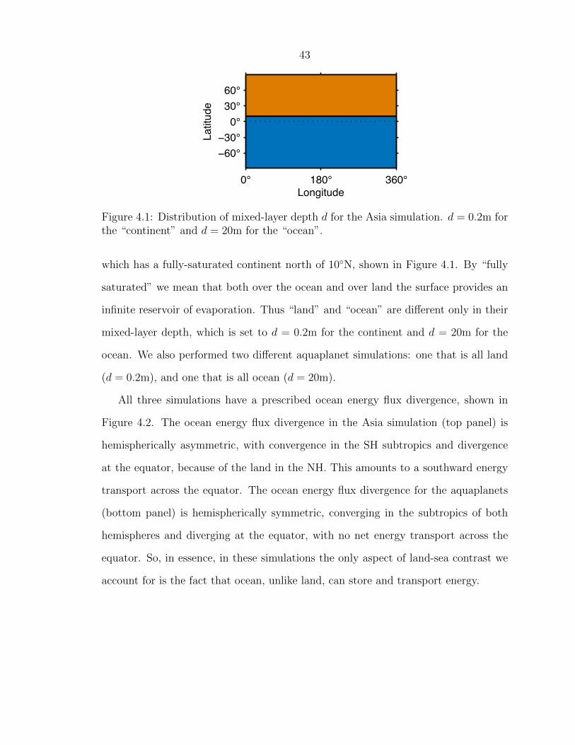
43

LongitudeLatitude

0° 180° 360°

−60°−30°0°30°60°

Figure 4.1: Distribution of mixed-layer depth d for the Asia simulation. d = 0.2m forthe “continent” and d = 20m for the “ocean”.

which has a fully-saturated continent north of 10N, shown in Figure 4.1. By “fully

saturated” we mean that both over the ocean and over land the surface provides an

infinite reservoir of evaporation. Thus “land” and “ocean” are different only in their

mixed-layer depth, which is set to d = 0.2m for the continent and d = 20m for the

ocean. We also performed two different aquaplanet simulations: one that is all land

(d = 0.2m), and one that is all ocean (d = 20m).

All three simulations have a prescribed ocean energy flux divergence, shown in

Figure 4.2. The ocean energy flux divergence in the Asia simulation (top panel) is

hemispherically asymmetric, with convergence in the SH subtropics and divergence

at the equator, because of the land in the NH. This amounts to a southward energy

transport across the equator. The ocean energy flux divergence for the aquaplanets

(bottom panel) is hemispherically symmetric, converging in the subtropics of both

hemispheres and diverging at the equator, with no net energy transport across the

equator. So, in essence, in these simulations the only aspect of land-sea contrast we

account for is the fact that ocean, unlike land, can store and transport energy.

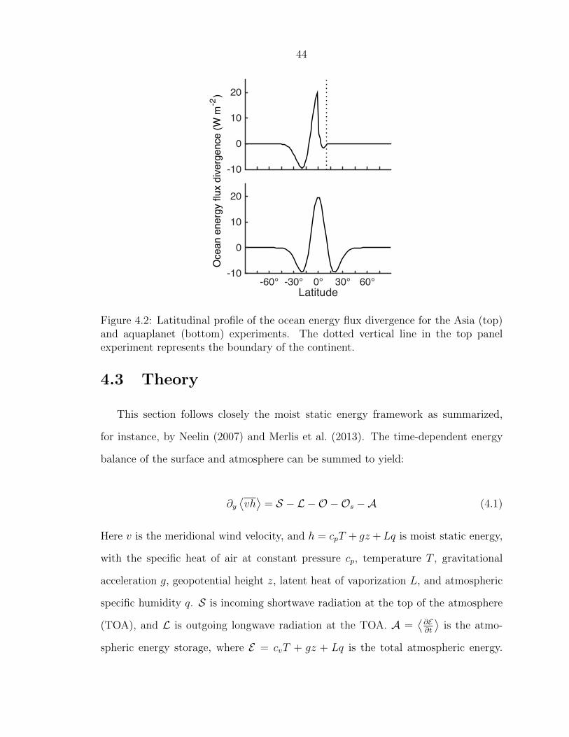
44

-10

0

10

20

Oce

an e

nerg

y flu

x di

verg

ence

(W m

-2)

Latitude-60° -30° 0° 30° 60°

-10

0

10

20

Figure 4.2: Latitudinal profile of the ocean energy flux divergence for the Asia (top)and aquaplanet (bottom) experiments. The dotted vertical line in the top panelexperiment represents the boundary of the continent.

4.3 Theory

This section follows closely the moist static energy framework as summarized,

for instance, by Neelin (2007) and Merlis et al. (2013). The time-dependent energy

balance of the surface and atmosphere can be summed to yield:

∂y⟨vh

⟩= S − L −O −Os −A (4.1)

Here v is the meridional wind velocity, and h = cpT + gz +Lq is moist static energy,

with the specific heat of air at constant pressure cp, temperature T , gravitational

acceleration g, geopotential height z, latent heat of vaporization L, and atmospheric

specific humidity q. S is incoming shortwave radiation at the top of the atmosphere

(TOA), and L is outgoing longwave radiation at the TOA. A =⟨∂E∂t

⟩is the atmo-

spheric energy storage, where E = cvT + gz + Lq is the total atmospheric energy.

45

〈·〉 denotes a mass-weighted vertical integral over the atmospheric column, and the

overbar denotes a zonal and temporal mean.

Here O = ∇ ·Fo is the divergence of the meridional ocean energy flux Fo which is

prescribed in our simulations (Fig. 4.2). The ocean energy storage is Os = cpoρod∂Ts∂t

,

with water density ρo, water heat capacity cpo, mixed-layer depth d and surface tem-

perature Ts. The surface energy budget is:

Os = SnetSFC − LnetSFC − LH − SH −∇ · Fo (4.2)

Here, LH and SH are the surface latent and sensible heat fluxes, respectively. Os is

negligible over land because of its small heat capacity, but not negligible over ocean

because it has a larger heat capacity and is therefore able to store energy. Note that

in much of the literature O + Os is known as the ocean heat uptake. Here we keep

these terms separate because the ocean energy flux divergence O does not vary on

seasonal timescales in our simulations, but the storage Os does.

Here we define the effective F net as the radiative and storage terms that must be

balanced by the horizontal atmospheric moist static energy flux divergence ∂y⟨vh

⟩

in the zonal mean:

F net = S − L −O −Os −A (4.3)

Note that in the conventional moist static energy framework (Neelin 2007), F net is

the net energy input to the atmospheric column, defined by the radiative and surface

fluxes at the upper and lower boundary of the column. Here there is a slight difference

in that we include the atmospheric storage term within F net, and we represent the

surface fluxes by the surface energy storage term Os.

Equations (4.1) and (4.3) tell us that the net energy input to the atmospheric

column must be balanced by the divergence of moist static energy in the atmosphere.

Thus the atmosphere responds to changes in energy input with changes in atmospheric

46

energy transport.

As done by Frierson and Hwang (2012), we integrate Eq. (4.1) in latitude to obtain⟨vh

⟩0

= 12

(F netSH − F net

NH ). Here the subscripts SH and NH denote integrals from the

equator to the pole in either hemisphere, and the subscript 0 indicates that the

quantity is evaluated at the equator. Thus the cross-equatorial atmospheric energy

flux⟨vh

⟩0

is proportional to the difference between the meridionally-integrated F net

in the two hemispheres.

In Bischoff and Schneider (2014) and Bischoff and Schneider (2015), a relation-

ship for the displacement of the ITCZ off the equator is derived using the column-

integrated atmospheric energy transport⟨vh

⟩. This energy transport in the tropics

is dominated by the upper branch of the Hadley circulation, and so the direction of

the transport tends to be in the direction of the mass flux in the upper branch. The

estimate for the ITCZ position is derived by assuming (1) that the ITCZ is located

where⟨vh

⟩changes sign (i.e., at the “energy flux equator” hereafter referred to as

the EFE) and (2) that⟨vh

⟩is linear between the equator and the EFE. This provides

a first-order estimate of the ITCZ position:

δ ≈ −1

a

⟨vh

⟩0

∂y⟨vh

⟩0

= −1

a

⟨vh

⟩0

S0 − L0 −O0 −Os0 −A0

(4.4)

Here δ is the displacement of the ITCZ off the equator, and a is the planetary radius.

Because we are considering seasonal cycles, the denominator explicitly accounts for

the atmospheric and oceanic heat storage, which is not included in the steady-state

simulations of Bischoff and Schneider (2014).

As shown in previous studies (e.g., Schneider et al. 2014; Adam et al. 2015),

the ITCZ is not always co-located with the energy flux equator, which is the first

assumption needed for Eq. (4.4) to hold. However, the ITCZ and EFE are correlated

both in structure and magnitude in our simulations.

47

The second assumption relies on the MSE flux being linear between the equator

and the EFE. This approximation holds either if the EFE is very close to the equator

or if the MSE flux is in fact linear. Even though the EFEs are displaced far from the

equator in our simulations, the fluxes are approximately linear in the tropics and so

this approximation holds well (Fig. 4.5).

Thus this theory states that the EFE, and thus the ITCZ, position depends on

both the cross-equatorial atmospheric energy flux⟨vh

⟩0

and the net energy input into

the equatorial atmosphere S0−L0−O0−Os0−A0. The denominator can be thought

of as a sensitivity parameter: When it is large, the ITCZ is relatively less sensitive to

changes in the cross-equatorial atmospheric energy flux, but when it is small, a slight

change in the cross-equatorial atmospheric energy flux can produce large excursions

in the ITCZ position. A change in either term by itself can produce a change in the

ITCZ position, and a change in both terms might not necessarily change the ITCZ

position. This theory was tested on idealized global and tropical warming simulations

in Bischoff and Schneider (2014) and Bischoff and Schneider (2015). Here, we extend

it to consider seasonal cycles.

4.4 GCM Results

The top panel of Figure 4.3 shows the distribution of precipitation in the Asia ex-

periment for JJA (June, July and August) and DJF (December, January and Febru-

ary) seasonal averages, and in the annual mean. In NH summer, there are two major

precipitation maxima, one over the continent around 23 and one just south of the

continent at 9. In SH summer, there is one large precipitation maximum located at

−12. The ITCZ in NH summer (over land) is located further poleward than in the

SH summer (over ocean), but more rain falls in the SH summer. In the annual mean,

the local maximum precipitation is located about 1 north of the equator, but the

48

0

4

8

12

16

NH summerSH summerANN

0

4

8

12

Prec

ipita

tion

(mm

day

-1)

Latitude-60° -30° 0° 30° 60°

0

4

8

12

Figure 4.3: Latitudinal distribution of precipitation in mm day−1 for the Asia (toppanel), “all ocean” aquaplanet (middle panel) and “all land” aquaplanet (bottompanel). Precipitation is shown for NH summer (red), SH summer (blue), and theannual mean (black). In the aquaplanet simulations, only one solstice season is shown(NH summer), because the two hemispheres are completely symmetric.

bulk of the precipitation falls south of the equator. Thus, we take the ITCZ to lie

just south of the equator at −5 in the annual mean, more in line with the center of

the precipitation distribution.

The bottom two panels show the annual-mean and summer precipitation for the

two aquaplanet simulations. In the “all ocean” aquaplanet, the average summer ITCZ

position is 6 from the equator, while in the “all land” aquaplanet the precipitation

maximum is located 27 from the equator during summer. There is also another pre-

cipitation maximum located at 10 in the “all land” aquaplanet. These two maxima

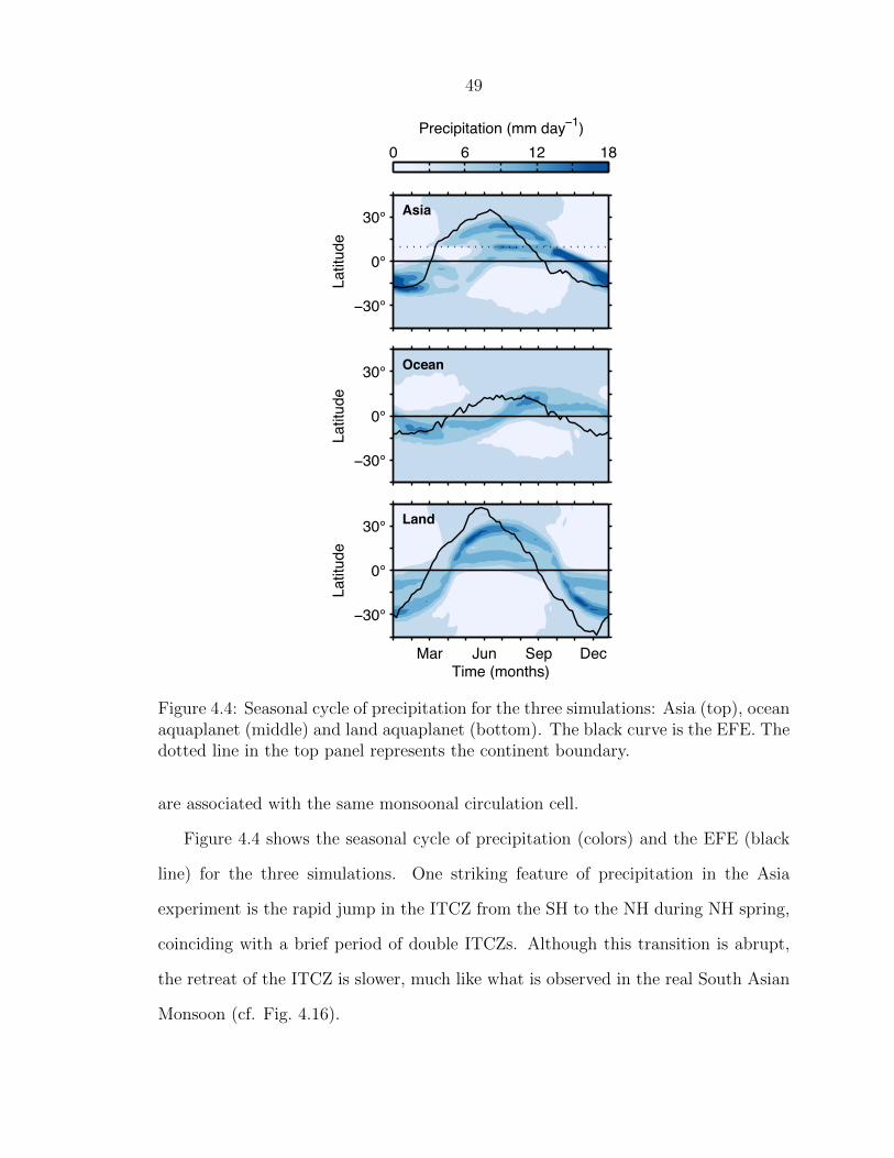
49

Asia

Latit

ude

−30°

0°

30°

Ocean

Latit

ude

−30°

0°

30°

Land

Time (months)

Latit

ude

Mar Jun Sep Dec

−30°

0°

30°

Precipitation (mm day−1)0 6 12 18

Figure 4.4: Seasonal cycle of precipitation for the three simulations: Asia (top), oceanaquaplanet (middle) and land aquaplanet (bottom). The black curve is the EFE. Thedotted line in the top panel represents the continent boundary.

are associated with the same monsoonal circulation cell.

Figure 4.4 shows the seasonal cycle of precipitation (colors) and the EFE (black

line) for the three simulations. One striking feature of precipitation in the Asia

experiment is the rapid jump in the ITCZ from the SH to the NH during NH spring,

coinciding with a brief period of double ITCZs. Although this transition is abrupt,

the retreat of the ITCZ is slower, much like what is observed in the real South Asian

Monsoon (cf. Fig. 4.16).

50

The ITCZ progression is relatively smooth for the aquaplanet simulations, with

the ITCZ and EFE migrating much further poleward for smaller values of the mixed-

layer depth d. For the “all land” simulation, the ITCZ reaches a maximum poleward

extent of 29, while in the “all ocean” simulation it only migrates a maximum of 12

from the equator.

Comparing the Asia and aquaplanet simulations reveals that the precipitation dis-

tribution for Asia is not just a superposition of the two aquaplanet simulations and

that, in fact, the hemispheric asymmetry in surface heat capacity has important and

nontrivial consequences on the tropical circulation and precipitation. The monsoonal

rainfall over the SH ocean in the Asia experiment reaches −19, which is 7 further

poleward than that in the “all ocean” experiment. On the other hand, the ascending

branch of the monsoonal circulation over the continent does not migrate as far pole-

ward as it does in the “all land” aquaplanet (25 for Asia versus 29 for “all land”).

These differences imply that there are some mechanisms arising from the hemispheric

asymmetry that shift the ITCZ further poleward in the SH summer and equatorward

in NH summer relative to the aquaplanet counterparts.

In the next two sections we strive to understand the hemispheric and temporal

asymmetries in the Asia simulation, using the aquaplanet simulations for reference.

4.5 Poleward boundary of ITCZ

4.5.1 Hemispheric energy imbalance

We want to determine what sets the poleward extent of monsoonal precipitation

both in the seasonal average and in the annual mean. To understand the differences

between the aquaplanet and Asia experiments, we turn to the atmospheric energy

budget Eq. (4.1). The Hadley circulation exists in the tropics in order to redistribute

energy on a differentially-heated planet. When we introduce a hemispheric asymmetry

51

→

→

→

↑↑↑

Latitude-60° -30° 0° 30° 60°

MSE

flux

(PW

)

-5

0

5

10 JJADJFANN

Figure 4.5: The vertically-integrated atmospheric energy flux⟨vh

⟩in JJA (red),

DJF (blue) and the annual mean (black) for the Asia simulation. Arrows pointinghorizontally indicate the value of the flux at the equator for each season. Arrowspointing vertically indicate the ITCZ location in each season.

in heat capacity, for example, it changes the distribution of energy (F net) and thus

the atmospheric energy transport by the Hadley circulation.

If there is no hemispheric asymmetry in the energy budget, a cross-equatorial

energy transport might not be needed. For example, if the planet is heated symmet-

rically (i.e., perpetual equinox), the ITCZ would remain at the equator and there

would be no mean cross-equatorial atmospheric energy flux. If the planet is hemi-

spherically symmetric and there is a seasonal cycle, we expect the annual mean ITCZ

to be right at the equator (e.g., the aquaplanet simulations). The excursions of the

ITCZ off the equator occur in the solstice seasons, in response to the hemispheric

asymmetry in solar insolation, and the atmosphere must transport energy across the

equator. The transport by the Hadley cell has the same sign as the mass flux in

the cell’s upper branch, to the extent that the effective energy stratification, or gross

moist stability, is positive. Since the aquaplanet is hemispherically and temporally

symmetric, these seasonal effects cancel out in the annual mean.

For the Asia experiment, however, there is an interhemispheric asymmetry in heat

capacity, which ultimately leads to the ITCZ (and EFE) being located in the SH in

the annual mean. Figure 4.5 shows the meridional MSE fluxes⟨vh

⟩for the Asia

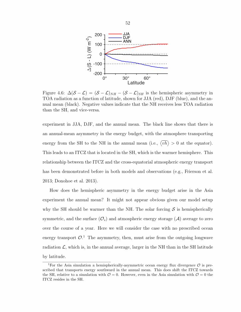
52

Latitude0° 30° 60°

∆(S

- L)

(W m

-2)

-200

-100

0

100

200 JJADJFANN

Figure 4.6: ∆(S − L) = (S − L)NH − (S − L)SH is the hemispheric asymmetry inTOA radiation as a function of latitude, shown for JJA (red), DJF (blue), and the an-nual mean (black). Negative values indicate that the NH receives less TOA radiationthan the SH, and vice-versa.

experiment in JJA, DJF, and the annual mean. The black line shows that there is

an annual-mean asymmetry in the energy budget, with the atmosphere transporting

energy from the SH to the NH in the annual mean (i.e.,⟨vh

⟩> 0 at the equator).

This leads to an ITCZ that is located in the SH, which is the warmer hemisphere. This

relationship between the ITCZ and the cross-equatorial atmospheric energy transport

has been demonstrated before in both models and observations (e.g., Frierson et al.

2013; Donohoe et al. 2013).

How does the hemispheric asymmetry in the energy budget arise in the Asia

experiment the annual mean? It might not appear obvious given our model setup

why the SH should be warmer than the NH. The solar forcing S is hemispherically

symmetric, and the surface (Os) and atmospheric energy storage (A) average to zero

over the course of a year. Here we will consider the case with no prescribed ocean

energy transport O.1 The asymmetry, then, must arise from the outgoing longwave

radiation L, which is, in the annual average, larger in the NH than in the SH latitude

by latitude.

1For the Asia simulation a hemispherically-asymmetric ocean energy flux divergence O is pre-scribed that transports energy southward in the annual mean. This does shift the ITCZ towardsthe SH, relative to a simulation with O = 0. However, even in the Asia simulation with O = 0 theITCZ resides in the SH.

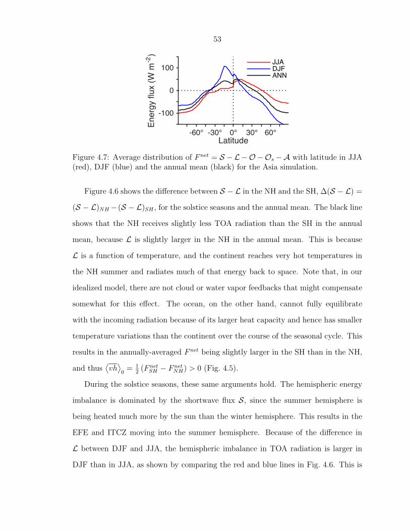
53

Latitude-60° -30° 0° 30° 60°

Ener

gy fl

ux (W

m-2

)

-100

0

100JJADJFANN

Figure 4.7: Average distribution of F net = S −L−O−Os−A with latitude in JJA(red), DJF (blue) and the annual mean (black) for the Asia simulation.

Figure 4.6 shows the difference between S − L in the NH and the SH, ∆(S − L) =

(S − L)NH− (S − L)SH , for the solstice seasons and the annual mean. The black line

shows that the NH receives slightly less TOA radiation than the SH in the annual

mean, because L is slightly larger in the NH in the annual mean. This is because

L is a function of temperature, and the continent reaches very hot temperatures in

the NH summer and radiates much of that energy back to space. Note that, in our

idealized model, there are not cloud or water vapor feedbacks that might compensate

somewhat for this effect. The ocean, on the other hand, cannot fully equilibrate

with the incoming radiation because of its larger heat capacity and hence has smaller

temperature variations than the continent over the course of the seasonal cycle. This

results in the annually-averaged F net being slightly larger in the SH than in the NH,

and thus⟨vh

⟩0

= 12

(F netSH − F net

NH) > 0 (Fig. 4.5).

During the solstice seasons, these same arguments hold. The hemispheric energy

imbalance is dominated by the shortwave flux S, since the summer hemisphere is

being heated much more by the sun than the winter hemisphere. This results in the

EFE and ITCZ moving into the summer hemisphere. Because of the difference in

L between DJF and JJA, the hemispheric imbalance in TOA radiation is larger in

DJF than in JJA, as shown by comparing the red and blue lines in Fig. 4.6. This is

54

consistent with the fact that the cross-equatorial energy flux⟨vh

⟩0

is larger in DJF

than in JJA (compare red and blue horizontal arrows in Fig. 4.5), even though F net

is not entirely determined by S − L, but also includes the effects of seasonal ocean

energy storage Os. The full F net is shown in Figure 4.7. The ocean energy storage

acts to balance out the hemispheric asymmetry in both JJA and DJF, since the ocean

stores heat in the summer and releases it back to the atmosphere during winter. The

atmospheric energy storage A has a negligible effect when averaged over a season.

Hence we arrive at an interesting outcome: the cross-equatorial atmospheric en-

ergy flux is larger in DJF, but the ITCZ reaches its most poleward position in JJA.

This result is at odds with previous work that suggests that the ITCZ position is lin-

early proportional to −⟨vh

⟩0

with a constant slope across a wide range of time scales

and forcings (Donohoe et al. 2013). As discussed in the next section, this apparent

contradiction is consistent with and explained by the theory presented in Section 4.3.

4.5.2 Quantitative estimates of the ITCZ position

While the arguments above allow for a qualitative understanding of the ITCZ

annual mean position and seasonal migrations, more quantitative understanding can

be achieved by using the theory of the ITCZ position recently developed by Bischoff

and Schneider (2014) and summarized in Section 4.3.

While our simulations do not adhere strictly to the two assumptions used to derive

Eq. (4.4), the EFE expansion provides a useful estimate for the ITCZ location. The

EFE does capture the fact that the ITCZ migrates further poleward in JJA than in

DJF, and that the ITCZ resides just south of the equator in the annual mean (cf.

Fig. 4.5). Thus it remains useful to use this framework for studying the location of

the monsoonal precipitation.

For the Asia simulation, in JJA, δ = 31 and the ITCZ is located at 23. For

DJF, δ = −21 and the ITCZ is located at −12. In the annual mean, δ = −4,

55

and the ITCZ is located around −5. This estimate is not perfect, but it captures

the most important feature of the seasonality in the Asia simulation: that the ITCZ

migrates further poleward in the NH summer than in the SH summer. For the “all

ocean” aquaplanet, δ = 10 in the summer and the ITCZ is located at 6. For “all

land” δ = 33 during summer and the ITCZ is located at 27.

Since the cross-equatorial atmospheric energy flux is larger in the SH summer,

but the ITCZ is positioned closer to the equator during this season, the denominator

of δ, F net0 = S0 − L0 − O0 − Os0 − A0, must be larger in DJF than in JJA. This is

indeed the case, as shown by Figure 4.7. This is an example of how the denominator

in Eq. (4.4) acts as a “sensitivity factor,” making it more or less easy to change the

ITCZ position for a given change in⟨vh

⟩0

(cf. Section 4.3, Bischoff and Schneider

2014). In DJF, the net energy input into the equatorial atmosphere is almost twice

as large as it is in JJA, so it only allows the ITCZ to move approximately half as far

as in JJA for every unit increase in the cross-equatorial energy flux.

Thus it is clear that in order to understand the seasonal position of the ITCZ,

we need to understand both the cross-equatorial energy transport⟨vh

⟩0

and its di-

vergence ∂y⟨vh

⟩0

= S0 − L0 − O0 − Os0 − A0.⟨vh

⟩0

can be understood from the

hemispheric asymmetry in F net, whereas understanding the energy flux divergence

requires more careful consideration of the atmospheric and surface energy budgets.

This analysis provokes the question: Why is F net0 so much larger in DJF than in

JJA? This will be discussed in detail in Section 4.6.2, where we look more closely at

the seasonal cycle of the cross-equatorial energy flux and its divergence.

56

4.6 Timing of Monsoon Onset/Retreat

4.6.1 Caveats

In this and the following sections, we use the atmospheric energy budget to inves-

tigate the timing of ITCZ shifts in NH and SH spring. There are a few caveats to this

approach. First, there is a conspicuous lag between the EFE and the ITCZ, such that

the EFE crosses the equator 30-120 days before the ITCZ does (depending on the

mixed-layer depth). The theory in Bischoff and Schneider (2014) assumes that the

two are co-located. This lag may be a model artifact, for it has been observed in the

CMIP3 models as well, but does not appear to be present in observations (Donohoe

et al. 2013; Chamales et al. 2015). However, because of the lag it is less obvious how

the arguments that explain the EFE position can be extended to account for the ITCZ

position in these simulations. More specifically, since there is a lag, there are times

when the ITCZ and the EFE are on opposite sides of the equator (cf. Fig. 4.4). This

means that the mass transport and the energy transport are in opposite directions

across the equator, which is reconciled by an adjustment of the gross moist stability

(GMS). This needs to be investigated further, but is beyond this scope of this re-

search. Despite these caveats, the seasonal cycle of the EFE well correlates with the

seasonal cycle of the ITCZ position, despite the time lag between the two. Hence, in

the rest of this section we will use the EFE as a proxy for the ITCZ.

Second, the theory assumes that eddy energy fluxes⟨v′h′

⟩are negligible at the

EFE location, so that the EFE is the zero of the mean energy flux. This is not

true at all times in our simulations. In fact, the eddy component of the flux is

important in the tropics, and sets the position of the EFE at some times. Surprisingly,

the latitude at which the eddy energy flux changes sign coincides with the ITCZ

at most times, while the latitude at which the mean energy flux changes sign is

not always correlated with the ITCZ. This goes against the widely-held notion that

57

the mean energy transport goes to zero at the boundary of the mean meridional

circulation. The mean energy flux does not always change sign at the ascending

branch, although that latitude is usually a point of minimum transport. We suspect

that these inconsistencies in our simulations arise from the vertical structure of the

circulation, in which ascent occurs along slanted streamlines in non-negligible portions

of the Hadley cell ascending branch, but more time must be dedicated to examining

the cause of this discrepancy.

Although the ITCZ crosses the equator early in NH spring, this transition is

not associated with the monsoon onset. In fact, a “double ITCZ” appears at this

time, with precipitation over the NH continent and over the SH tropical ocean. If

we consider the monsoon to be a deep, cross-equatorial circulation with ascending

branch in the summer hemisphere subtropics and descending branch in the opposite

hemisphere, in agreement with many studies, the monsoon onset only occurs in June.

The early NH spring transition is instead associated with the development of a local,

linear and narrow cell over the continent, as described in Section 4.6.4.1. The SH

spring is characterized by a gradual and smoothly-shifting ITCZ.

The fact that there is a NH ITCZ/EFE transition that does not coincide with

monsoon onset means the energy budget framework will be less useful for looking at

NH monsoon onset. The occurrence of this secondary transition is a limitation of

our model setup, and will be discussed below. Nonetheless, the early transition of

the ITCZ from the southern to the northern hemisphere (and the onset of the double

ITCZ) is still an interesting feature in our simulation, and we want to understand

what controls its timing. In the following, “monsoon onset” will therefore refer to

the onset of a deep and cross-equatorial winter cell in June while “NH EFE/ITCZ

transition” refers to the rapid shift in the EFE from the SH to the NH in March.

The next section will discuss the ITCZ shifts and Section 4.6.5 will discuss the NH

monsoon onset.

58

4.6.2 Energy budget and ITCZ shifts

Figure 4.4 shows the energy flux equator⟨vh

⟩= 0 (black line in each panel), or

EFE, as a function of time for the three experiments. For Asia, the EFE exhibits the

same rapid onset and slow retreat pattern as the ITCZ, albeit shifted by ≈ 30 days.

We want to understand what makes the NH and SH EFE transition so different in

boreal and austral spring, with a rapid transition from the SH to the NH in March and

a more gradual shift back to the SH in September. Using Eq. (4.4), the two quantities

that define the EFE position are the cross-equatorial atmospheric energy flux⟨vh

⟩0

and the net energy input to the equatorial atmosphere ∂y⟨vh

⟩0≈ S0−L0−O0−Os0.

Changes in either one of these terms over the course of the seasonal cycle could

produce asymmetries in the timing of the EFE progression. Note that here we have

neglected A0 because it is much smaller than the other terms, however it is included

in all calculations.

The seasonal cycle of these two terms is plotted in Fig. 4.8 for all three exper-

iments. The “transition period,” when the EFE shifts from one hemisphere to the

other, is shaded for each simulation. This is taken as the period beginning 10 days

before and ending 10 days after the EFE crosses the equator. Blue arrows indicate

the time of monsoon onset, defined as the development of a deep, cross-equatorial

circulation, and red arrows indicate the beginning of the brief double-ITCZ period

during NH spring.

The cross-equatorial atmospheric energy flux⟨vh

⟩0

exhibits an asymmetry in its

temporal structure between the two transition periods, although not as dramatic

as the EFE, with⟨vh

⟩0

changing more rapidly in the SH-NH transition and more

slowly in the NH-SH transition (top left panel, compare slopes of the lines near the

shaded region). The asymmetry comes from a combination of temporal asymmetries

in the surface and atmospheric energy storage terms. In general the hemispheric

asymmetry in F net, ∆F net, is dominated by ∆(S − L), which is temporally symmetric

59

↑↑ ↑

Asia

−⟨vh⟩0 (PW)

-8-4048

↑↑ ↑

∂y⟨vh⟩0 (Wm−2)

0

100

↑↑

Ocean

-8-4048

↑↑0

100

↑ ↑

Land

Time (months)Mar Jun Sep Dec

-8-4048

↑ ↑

Time (months)Mar Jun Sep Dec

0

100

Figure 4.8: Seasonal cycle of the atmospheric energy flux at the equator (left) andits divergence (right). Three simulations are shown: The Asia simulation (top row),the 20-m aquaplanet (middle row) and the 0.2-m aquaplanet (bottom row). Thetwo terms plotted are the numerator and denominator of δ in Eq. (4.4), respectively.Shading represents the transition time, during which the EFE crosses the equator.Blue arrows indicate monsoon onset, as defined by the development of a deep, cross-equatorial circulation. The red arrows in the top panel indicate the beginning of thebrief double-ITCZ period during NH spring for the Asia simulation.

60

and changes more rapidly than⟨vh

⟩0. Here the ∆ refers to the difference between the

SH and NH. In the NH spring the storage terms have a small effect on⟨vh

⟩0, allowing

the hemispheric asymmetry to change rapidly like ∆(S − L). In SH spring they have

a larger effect, causing⟨vh

⟩0

to change less rapidly. At least for the Asia simulation

(and possibly the ocean simulation as well), the monsoon onset (blue arrows) seems

to occur immediately following a rapid increase in⟨vh

⟩0.

The divergence of this flux, or the net energy input to the equatorial atmosphere,

has approximately the same value in the transition periods, but has a more temporally

asymmetric structure than⟨vh

⟩0

(top right panel). This term changes sign when it

starts raining over the NH continent, at the onset of the double ITCZ (red arrow). At

the point when ∂y⟨vh

⟩0

= 0, the linear approximation breaks down and higher order

terms in the Taylor expansion are needed and the precipitation distribution shows a

propensity for a double ITCZ structure (Bischoff and Schneider 2015). Before and

after this period the linear approximation holds and the divergence is small, allowing

the EFE to shift relatively quickly and relatively far, farther than it does in SH

summer. After the SH spring EFE transition, on the other hand, ∂y⟨vh

⟩0

rapidly

increases, making it difficult to move the EFE, and causing the ITCZ to shift more

slowly around the time of monsoon onset.

In the “all ocean” and “all land” aquaplanet simulations, ∂y⟨vh

⟩0

is temporally

symmetric, and the EFE transitions occur when the net energy input is decreasing

toward its minimum value (bottom two rows of Fig. 4.8). Like for the Asia simulation,

F net decreases to zero for the 20-m aquaplanet simulation after the EFE crosses the

equator but right before the ITCZ crosses the equator.

It is the ratio of the cross-equatorial energy flux⟨vh

⟩0

and the net energy input

to the equatorial atmosphere ∂y⟨vh

⟩0

that defines the EFE position (4.4). Thus

Figure 4.8 shows that, for land, the EFE position can be explained almost entirely by

the cross-equatorial energy flux (Fig. 4.8 left column), since the net energy input to

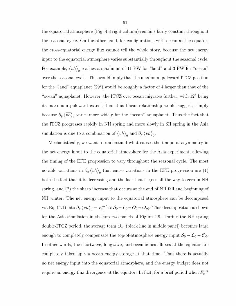
61

the equatorial atmosphere (Fig. 4.8 right column) remains fairly constant throughout

the seasonal cycle. On the other hand, for configurations with ocean at the equator,

the cross-equatorial energy flux cannot tell the whole story, because the net energy

input to the equatorial atmosphere varies substantially throughout the seasonal cycle.

For example,⟨vh

⟩0

reaches a maximum of 11 PW for “land” and 3 PW for “ocean”

over the seasonal cycle. This would imply that the maximum poleward ITCZ position

for the “land” aquaplanet (29) would be roughly a factor of 4 larger than that of the

“ocean” aquaplanet. However, the ITCZ over ocean migrates further, with 12 being

its maximum poleward extent, than this linear relationship would suggest, simply

because ∂y⟨vh

⟩0

varies more widely for the “ocean” aquaplanet. Thus the fact that

the ITCZ progresses rapidly in NH spring and more slowly in SH spring in the Asia

simulation is due to a combination of⟨vh

⟩0

and ∂y⟨vh

⟩0.

Mechanistically, we want to understand what causes the temporal asymmetry in

the net energy input to the equatorial atmosphere for the Asia experiment, allowing

the timing of the EFE progression to vary throughout the seasonal cycle. The most

notable variations in ∂y⟨vh

⟩0

that cause variations in the EFE progression are (1)

both the fact that it is decreasing and the fact that it goes all the way to zero in NH

spring, and (2) the sharp increase that occurs at the end of NH fall and beginning of

NH winter. The net energy input to the equatorial atmosphere can be decomposed

via Eq. (4.1) into ∂y⟨vh

⟩0

= F net0 ≈ S0−L0−O0−Os0. This decomposition is shown

for the Asia simulation in the top two panels of Figure 4.9. During the NH spring

double-ITCZ period, the storage term Os0 (black line in middle panel) becomes large

enough to completely compensate the top-of-atmosphere energy input S0 −L0 −O0.

In other words, the shortwave, longwave, and oceanic heat fluxes at the equator are

completely taken up via ocean energy storage at that time. Thus there is actually

no net energy input into the equatorial atmosphere, and the energy budget does not

require an energy flux divergence at the equator. In fact, for a brief period when F net0

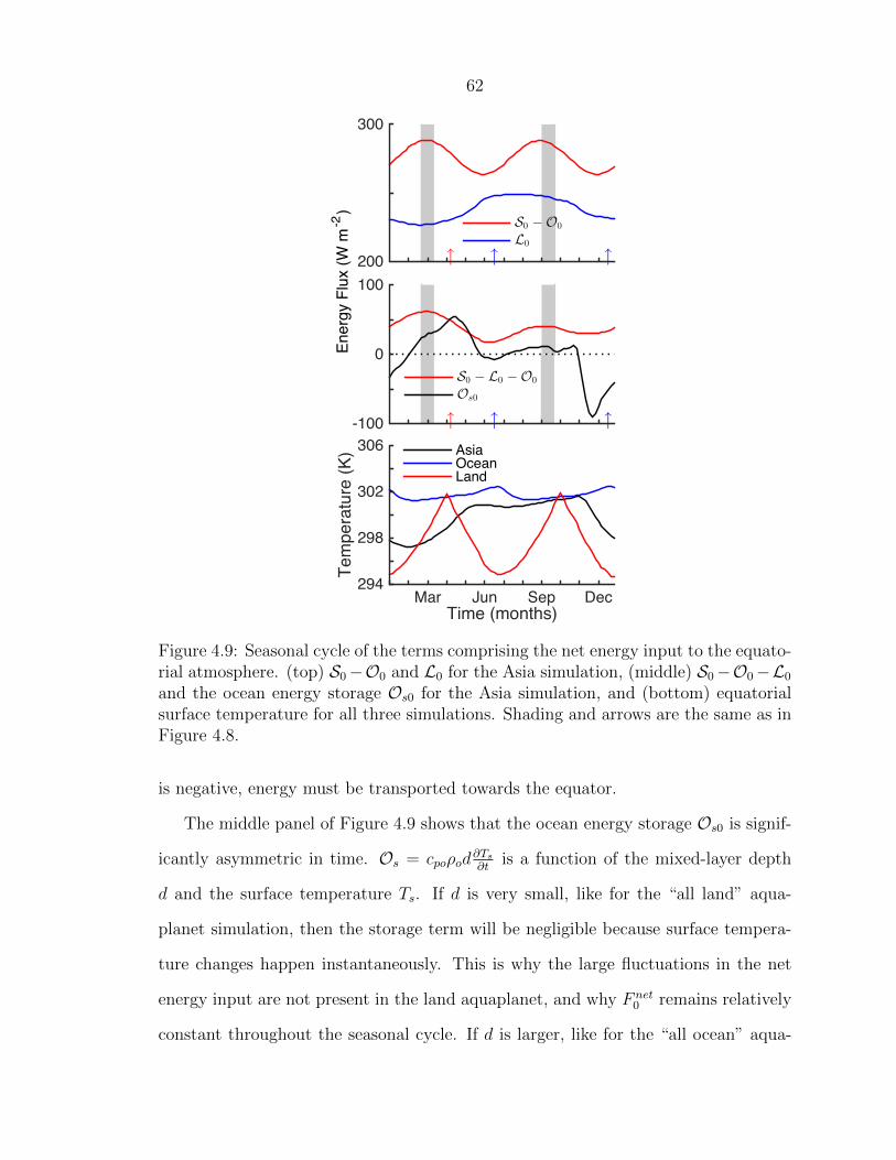
62

↑↑ ↑200

300

S0 −O0

L0

↑↑ ↑

Ener

gy F

lux

(W m

-2)

-100

0

100

S0 − L0 −O0

Os0

Time (months)Mar Jun Sep Dec

Tem

pera

ture

(K)

294

298

302

306 AsiaOceanLand

Figure 4.9: Seasonal cycle of the terms comprising the net energy input to the equato-rial atmosphere. (top) S0−O0 and L0 for the Asia simulation, (middle) S0−O0−L0

and the ocean energy storage Os0 for the Asia simulation, and (bottom) equatorialsurface temperature for all three simulations. Shading and arrows are the same as inFigure 4.8.

is negative, energy must be transported towards the equator.

The middle panel of Figure 4.9 shows that the ocean energy storage Os0 is signif-

icantly asymmetric in time. Os = cpoρod∂Ts∂t

is a function of the mixed-layer depth

d and the surface temperature Ts. If d is very small, like for the “all land” aqua-

planet simulation, then the storage term will be negligible because surface tempera-

ture changes happen instantaneously. This is why the large fluctuations in the net

energy input are not present in the land aquaplanet, and why F net0 remains relatively

constant throughout the seasonal cycle. If d is larger, like for the “all ocean” aqua-

63

planet, then Os is associated with the seasonal cycle of surface temperature. Thus the

same compensation between S0−L0−O0 and Os0 can occur for the ocean aquaplanet,

causing F net0 to go to zero for a brief period twice during the seasonal cycle.

The equatorial surface temperature is plotted in the bottom panel of Figure 4.9 for

all three simulations. If we compare the Asia simulation with the ocean aquaplanet,

we see that in JJA their equatorial surface temperatures look very similar, but in DJF

the surface temperatures for Asia are much lower than that of the 20-m aquaplanet.

In other words, for Asia the storage term becomes large and negative in SH spring

because there is a large cooling of the equatorial ocean, which corresponds to a release

of heat from the ocean to the atmosphere. The ocean takes up heat in NH spring

when the equatorial surface warms back up.

The seasonal cycle of surface temperature sets both the storage term (if the surface

heat capacity is sufficiently large) and also the OLR L in our model. L is closely tied

to surface temperature because there are no cloud or water vapor feedbacks in this

idealized model to allow re-absorption of that radiation within the atmosphere, and

therefore it must be emitted back to space. Because Ts0 has a single peak in the Asia

simulation, L0 does too (top panel of Fig. 4.9). The structure of Os0, with ocean heat

storage in NH spring and ocean heat release in SH spring, also corresponds to the

pattern of surface temperature variations.

So the question becomes, why does the equatorial surface temperature have a

single peak in the seasonal cycle of the Asia simulation, whereas the two aquaplanets

have a double-peak structure? The equatorial SSTs in the Asia simulation can be

compared with the “all ocean” aquaplanet because both of them have a 20-m mixed-

layer depth at the equator. The pattern of Ts for Asia is similar to that in the “ocean”

aquaplanet during NH summer and fall, but there is a significant cooling that occurs

in NH winter that causes departures from the “ocean” case. In the following sections,

we explain how dynamics plays a role in creating this temporal asymmetry in the

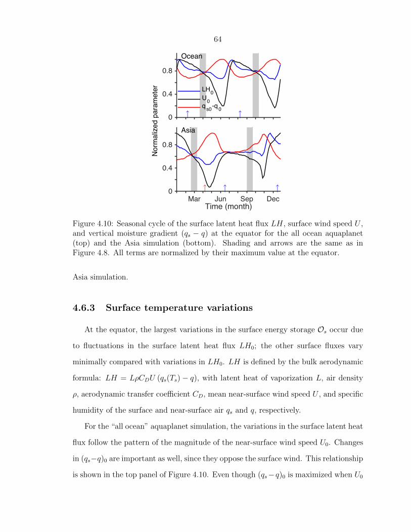
64

↑↑

Ocean

0

0.4

0.8

LH0U0qs0-q0

↑↑ ↑

Asia

Nor

mal

ized

par

amet

er

Time (month)Mar Jun Sep Dec

0

0.4

0.8

Figure 4.10: Seasonal cycle of the surface latent heat flux LH, surface wind speed U ,and vertical moisture gradient (qs − q) at the equator for the all ocean aquaplanet(top) and the Asia simulation (bottom). Shading and arrows are the same as inFigure 4.8. All terms are normalized by their maximum value at the equator.

Asia simulation.

4.6.3 Surface temperature variations

At the equator, the largest variations in the surface energy storage Os occur due

to fluctuations in the surface latent heat flux LH0; the other surface fluxes vary

minimally compared with variations in LH0. LH is defined by the bulk aerodynamic

formula: LH = LρCDU (qs(Ts)− q), with latent heat of vaporization L, air density

ρ, aerodynamic transfer coefficient CD, mean near-surface wind speed U , and specific

humidity of the surface and near-surface air qs and q, respectively.

For the “all ocean” aquaplanet simulation, the variations in the surface latent heat

flux follow the pattern of the magnitude of the near-surface wind speed U0. Changes

in (qs−q)0 are important as well, since they oppose the surface wind. This relationship

is shown in the top panel of Figure 4.10. Even though (qs−q)0 is maximized when U0

65

is at a minimum, LH0 qualitatively follows the pattern of U0. The equatorial surface

wind speed maximizes in mid-summer just after the ITCZ crosses the equator, when

the circulation becomes cross-equatorial. This is also around the time when LH0

maximizes, cooling the surface and warming the atmosphere. LH0 maximizes slightly

earlier than the surface wind speed because of the coupling between the surface wind

and the moisture gradient.

LH0 in the Asia experiment also qualitatively follows U0. Because there is a

significant temporal asymmetry in the surface wind speed, there is also an asymmetry

in LH0. U0 is about 60% weaker in NH spring/summer than in SH spring/summer.

This leads to a much larger cooling of equatorial SSTs in SH spring than in NH

spring and is the reason for the single peak structure in SST. There is also a slight

difference in phasing between (qs−q)0 and U0 between NH spring and SH spring, which

causes LH0 to be approximately constant during NH summer instead of reaching a

maximum value in early summer. This phasing difference has a smaller effect than

the surface wind on the equatorial cooling; if it did not occur, LH0 would reach a

smaller maximum value than in SH spring and the cooling that would result would

be small compared with that in SH spring. Thus, the SST would still basically have

one maximum.

Figure 4.10 does not provide information about the magnitude of the quantities

plotted, so the values of LH0 between the Asia and aquaplanet simulations cannot be

compared. However, the magnitude of the latent heating that occurs in November in

the Asia simulation is much larger than that in the aquaplanet simulation, which can

be attributed to the stronger surface winds during SH spring in the Asia experiment

than in the aquaplanet. This is why the surface temperature drops so much more in

SH spring for the Asia experiment (e.g., bottom panel of Fig. 4.9).

Thus we have found that a seasonal asymmetry in the surface winds produces an

asymmetry in the latent heat flux which, in turn, gives an asymmetry in the surface

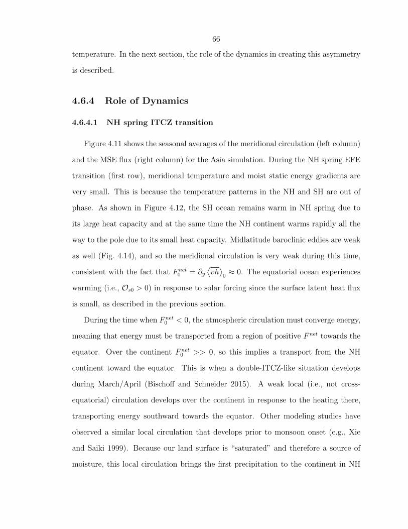
66

temperature. In the next section, the role of the dynamics in creating this asymmetry

is described.

4.6.4 Role of Dynamics

4.6.4.1 NH spring ITCZ transition

Figure 4.11 shows the seasonal averages of the meridional circulation (left column)

and the MSE flux (right column) for the Asia simulation. During the NH spring EFE

transition (first row), meridional temperature and moist static energy gradients are

very small. This is because the temperature patterns in the NH and SH are out of

phase. As shown in Figure 4.12, the SH ocean remains warm in NH spring due to

its large heat capacity and at the same time the NH continent warms rapidly all the

way to the pole due to its small heat capacity. Midlatitude baroclinic eddies are weak

as well (Fig. 4.14), and so the meridional circulation is very weak during this time,

consistent with the fact that F net0 = ∂y

⟨vh

⟩0≈ 0. The equatorial ocean experiences

warming (i.e., Os0 > 0) in response to solar forcing since the surface latent heat flux

is small, as described in the previous section.

During the time when F net0 < 0, the atmospheric circulation must converge energy,

meaning that energy must be transported from a region of positive F net towards the

equator. Over the continent F net0 >> 0, so this implies a transport from the NH

continent toward the equator. This is when a double-ITCZ-like situation develops

during March/April (Bischoff and Schneider 2015). A weak local (i.e., not cross-

equatorial) circulation develops over the continent in response to the heating there,

transporting energy southward towards the equator. Other modeling studies have

observed a similar local circulation that develops prior to monsoon onset (e.g., Xie

and Saiki 1999). Because our land surface is “saturated” and therefore a source of

moisture, this local circulation brings the first precipitation to the continent in NH

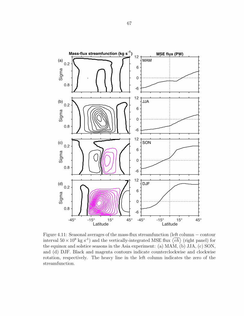
67

(a)Mass-flux streamfunction (kg s-1)

Sigm

a0.2

0.8

MAMMSE flux (PW)

-6

0

6

12

(b)

Sigm

a

0.2

0.8

JJA

-6

0

6

12

(c)

Sigm

a

0.2

0.8

SON

-6

0

6

12

(d)

Latitude-45° -15° 15° 45°

Sigm

a

0.2

0.8

DJF

Latitude-45° -15° 15° 45°

-6

0

6

12

Figure 4.11: Seasonal averages of the mass-flux streamfunction (left column− contourinterval 50× 109 kg s-1) and the vertically-integrated MSE flux

⟨vh

⟩(right panel) for

the equinox and solstice seasons in the Asia experiment: (a) MAM, (b) JJA, (c) SON,and (d) DJF. Black and magenta contours indicate counterclockwise and clockwiserotation, respectively. The heavy line in the left column indicates the zero of thestreamfunction.

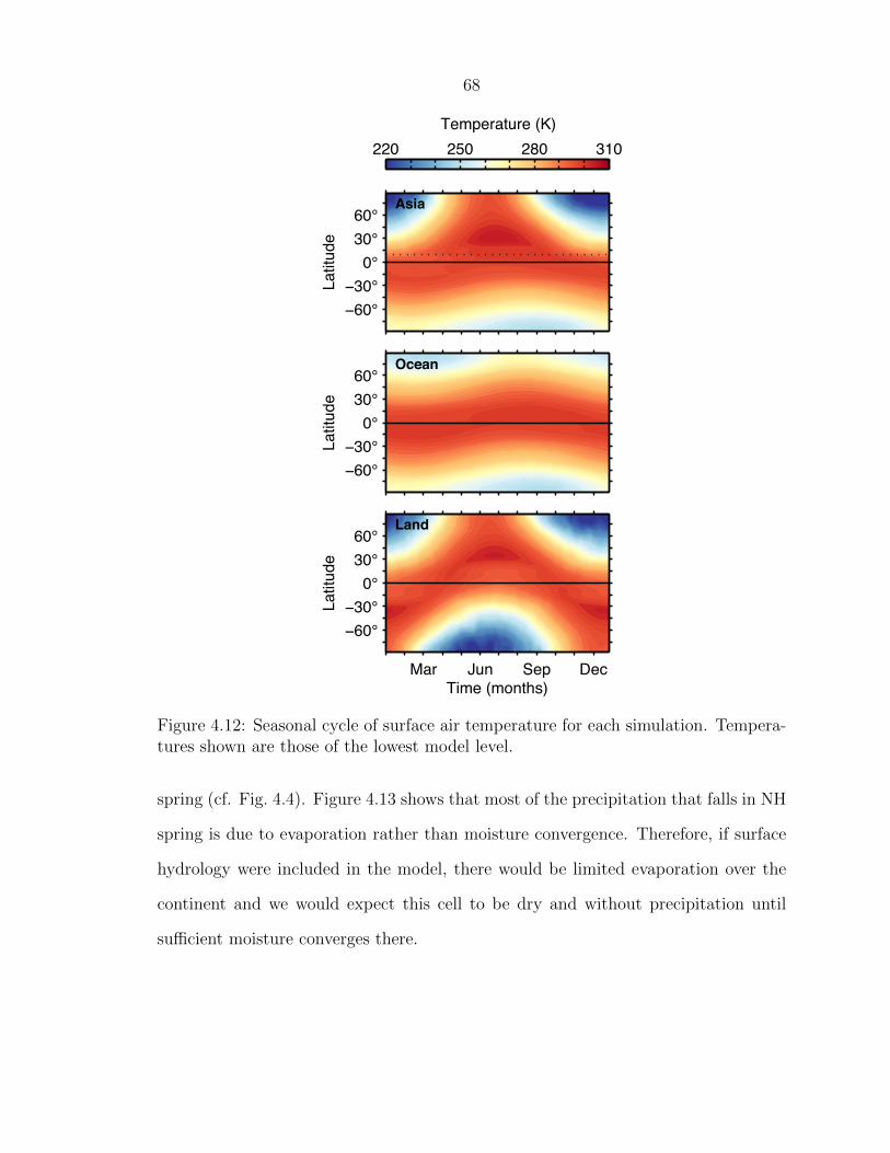
68

Asia

Latit

ude

−60°−30°

0°30°60°

Ocean

Latit

ude

−60°−30°

0°30°60°

Land

Time (months)

Latit

ude

Mar Jun Sep Dec

−60°−30°

0°30°60°

Temperature (K)220 250 280 310

Figure 4.12: Seasonal cycle of surface air temperature for each simulation. Tempera-tures shown are those of the lowest model level.

spring (cf. Fig. 4.4). Figure 4.13 shows that most of the precipitation that falls in NH

spring is due to evaporation rather than moisture convergence. Therefore, if surface

hydrology were included in the model, there would be limited evaporation over the

continent and we would expect this cell to be dry and without precipitation until

sufficient moisture converges there.

69

Time (months)La

titud

e

Mar Jun Sep Dec

−30°

0°

30°

(P−E)/P0 .4 .8

Figure 4.13: Fraction of precipitation owing to moisture flux convergence, (P−E)/P ,for the Asia simulation. P and E are precipitation and evaporation, respectively.

4.6.4.2 SH spring ITCZ transition

The SH spring transition looks very different (third row of Fig. 4.11). During this

time, the NH winter cell starts to strengthen rapidly. The continent cools off quickly,

increasing the pole-equator temperature gradient and thus the baroclinic eddy activity

in the NH extratropics. The strength of these eddies is linked to the strength of

the Hadley circulation through the zonally-averaged zonal momentum budget f(1−

Ro)v ≈ S, with Coriolis parameter f , local Rossby number Ro = −ζ/f , relative

vorticity ζ and eddy momentum flux divergence S = ∂y(u′v′ cosφ). Figure 4.14 shows

the vertically-integrated eddy momentum flux divergence (EMFD) as a function of

time and latitude for all three simulations. For Asia (top panel), the EMFD increases

rapidly in SH spring over the continent and the circulation strengthens linearly with

it until SH winter, which is when the cell becomes more constrained by the energy

budget (Bordoni and Schneider 2008; Schneider and Bordoni 2008).

Also during this time, the atmospheric energy transport begins to increase rapidly

(cf. Fig. 4.8). This implies that more energy is being transported from the SH to the

NH as this cell strengthens and moves further into the SH.

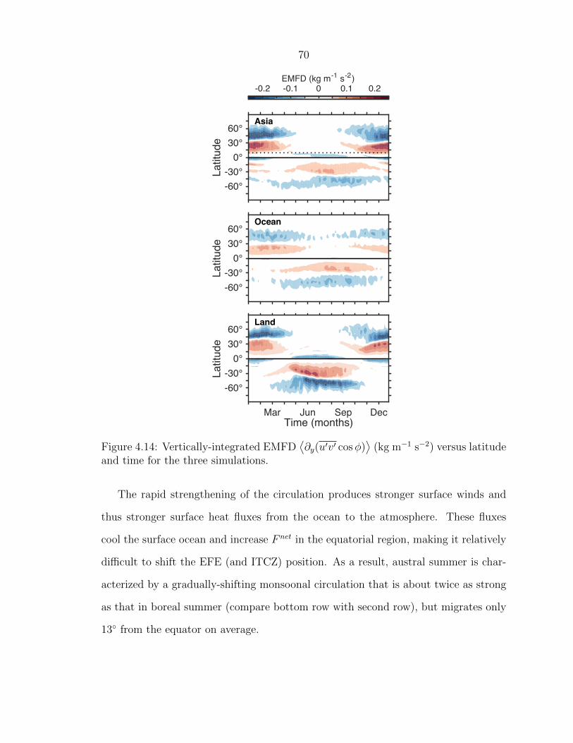
70

Asia

Latit

ude

-60°-30°

0°30°60°

OceanLa

titud

e

-60°-30°

0°30°60°

Land

Time (months)Mar Jun Sep Dec

Latit

ude

-60°-30°

0°30°60°

EMFD (kg m-1 s-2)-0.2 -0.1 0 0.1 0.2

Figure 4.14: Vertically-integrated EMFD⟨∂y(u′v′ cosφ)

⟩(kg m−1 s−2) versus latitude

and time for the three simulations.

The rapid strengthening of the circulation produces stronger surface winds and

thus stronger surface heat fluxes from the ocean to the atmosphere. These fluxes

cool the surface ocean and increase F net in the equatorial region, making it relatively

difficult to shift the EFE (and ITCZ) position. As a result, austral summer is char-

acterized by a gradually-shifting monsoonal circulation that is about twice as strong

as that in boreal summer (compare bottom row with second row), but migrates only

13 from the equator on average.

71

4.6.5 NH monsoon onset

Figure 4.15 shows the formation and evolution of a local cell at the continent edge

at day 100 (i.e., in April). The development of this circulation is associated with a

small and negative F net in the tropics, indicating that energy needs to be transported

towards the equator.

As the SH begins to cool and the pole-equator temperature gradient strengthens

there, midlatitude baroclinic eddies drive a weak circulation in the SH subtropics.

Thus around day 120 there are actually two separate cells that are rotating in the

same sense, which can be seen in the second row of Figure 4.15. This southern cell

is the source of the other band of precipitation that does not cross the equator until

June (cf. Fig. 4.4).

These two circulations coexist and eventually merge during summer, forming one

cross-equatorial monsoonal cell that transports energy southward. The merging of

the two cells occurs as a negative absolute vorticity gradient develops in the upper

troposphere over the continent around day 135 (right panel of Fig. 4.15). Such a

rapid onset of a monsoonal circulation is similar to that described by Plumb and Hou

(1992) and Emanuel (1995) for axisymmetric atmospheres, and can only occur when

the low-level moist entropy gradients exceed a threshold value.

4.7 Discussion

4.7.1 Relation to other theories

In the literature, it has been suggested that the ITCZ position is linearly pro-

portional to the cross-equatorial energy flux (e.g., Donohoe et al. 2013). In the Asia

simulation, the magnitude of the cross-equatorial atmospheric energy flux is larger in

DJF than in JJA (Fig. 4.5). Thus, under the assumption that δ ∼⟨vh

⟩0, the ITCZ

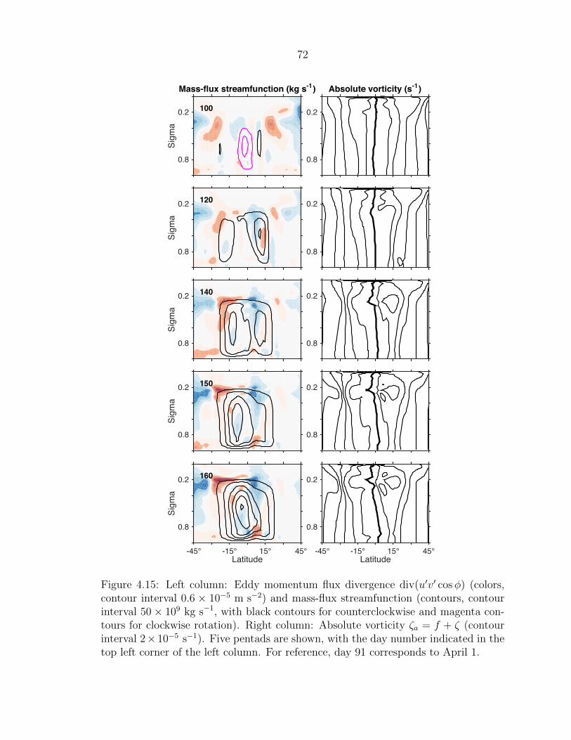
72

100

Mass-flux streamfunction (kg s-1)

Sigm

a

0.2

0.8

Absolute vorticity (s-1)

0.2

0.8

120

Sigm

a

0.2

0.8

0.2

0.8

140

Sigm

a

0.2

0.8

0.2

0.8

150

Sigm

a

0.2

0.8

0.2

0.8

160

Latitude-45° -15° 15° 45°

Sigm

a

0.2

0.8

Latitude-45° -15° 15° 45°

0.2

0.8

Figure 4.15: Left column: Eddy momentum flux divergence div(u′v′ cosφ) (colors,contour interval 0.6 × 10−5 m s−2) and mass-flux streamfunction (contours, contourinterval 50× 109 kg s−1, with black contours for counterclockwise and magenta con-tours for clockwise rotation). Right column: Absolute vorticity ζa = f + ζ (contourinterval 2× 10−5 s−1). Five pentads are shown, with the day number indicated in thetop left corner of the left column. For reference, day 91 corresponds to April 1.

73

should be located further poleward in DJF than in JJA, but that is not what we

see. In fact, the JJA ITCZ is 8 further poleward. This means that, at least in an

idealized setting such as this one, seasonal changes of F net0 (and specifically surface en-

ergy storage) matter for setting the ITCZ location. This also implies that the energy

transport by the Hadley circulation is larger in DJF than in JJA, even though the

cell itself is smaller in extent. This is in disagreement with axisymmetric theories of

cross-equatorial Hadley cells (Lindzen and Hou 1988), albeit not very surprising since

these axisymmetric models have fixed meridional pole-equator temperature gradients

and static stability.

In the Asia case, it is the ocean energy storage that can close the gap between

S0 − L0 and zero, causing ∂y⟨vh

⟩0

to become very small2. This can only happen if

there is a large surface heat capacity at the equator. Otherwise, theoretically there

could be the same surface temperature pattern, but no ocean energy storage. In this

case, there would still be a temporal asymmetry in F net0 due to L0, but F net

0 would

not be as temporally asymmetric and it would not go to zero. In this hypothetical

case, F net0 ≈ S0 − L0 would be the denominator of the EFE position δ, and it would

still be larger in DJF than in JJA (cf. Fig. 4.9), which by itself would have the effect

of shifting the ITCZ poleward in JJA and equatorward in DJF, just like in the Asia

experiment. During the monsoon onset it would also have the same effect, S0−L0 is

smaller for NH monsoon onset than for SH monsoon onset (cf. Fig. 4.9, blue arrows).

4.7.2 Comparison to observations and CMIP5

While very idealized, the results from our simulations bear resemblance to the

seasonal cycle of precipitation in the Indian monsoon sector. Figure 4.16 shows the

seasonal cycle of precipitation from TRMM daily data (top panel) and the CMIP5

2Note that in our idealized experiments, O0 is prescribed and constant in time. Therefore weomit it from this discussion of a hypothetical experiment.

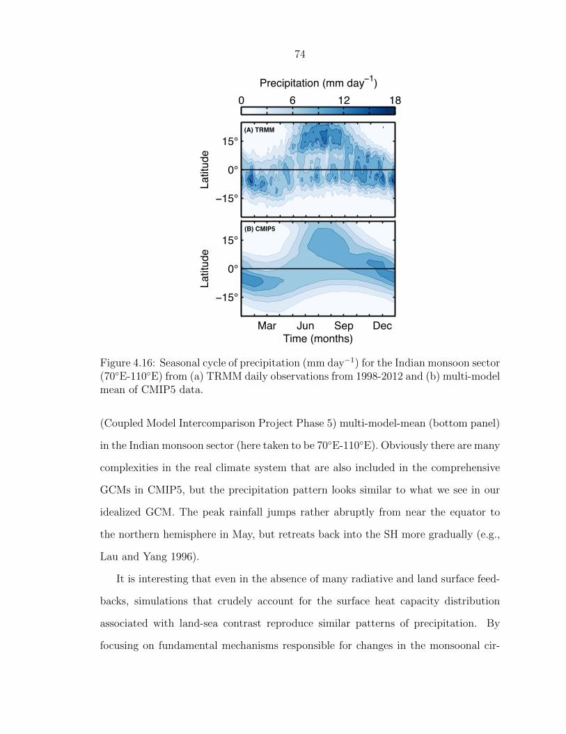
74

(B) CMIP5

Time (months)

Latit

ude

Mar Jun Sep Dec

−15°

0°

15°

(A) TRMM

Latit

ude

−15°

0°

15°

Precipitation (mm day−1)0 6 12 18

Figure 4.16: Seasonal cycle of precipitation (mm day−1) for the Indian monsoon sector(70E-110E) from (a) TRMM daily observations from 1998-2012 and (b) multi-modelmean of CMIP5 data.

(Coupled Model Intercomparison Project Phase 5) multi-model-mean (bottom panel)

in the Indian monsoon sector (here taken to be 70E-110E). Obviously there are many

complexities in the real climate system that are also included in the comprehensive

GCMs in CMIP5, but the precipitation pattern looks similar to what we see in our

idealized GCM. The peak rainfall jumps rather abruptly from near the equator to

the northern hemisphere in May, but retreats back into the SH more gradually (e.g.,

Lau and Yang 1996).

It is interesting that even in the absence of many radiative and land surface feed-

backs, simulations that crudely account for the surface heat capacity distribution

associated with land-sea contrast reproduce similar patterns of precipitation. By

focusing on fundamental mechanisms responsible for changes in the monsoonal cir-

75

culation and precipitation, it is expected that this work can provide insight into and

more robustly constrain present-day simulations (and possibly future projections) of

Earth’s monsoons by state-of-the-art climate models in the CMIP5 archive.

4.8 Conclusions

This work illustrates that both spatial and temporal symmetry breaking of mon-

soonal precipitation patterns can occur in an idealized model with hemispherically

asymmetric continental geometry.

The spatial symmetry is broken because of the hemispheric energy imbalance

imposed by the asymmetry in surface heat capacity. Interestingly, the ITCZ mi-

grates further poleward in JJA, even though the cross-equatorial energy transport

is maximized in DJF. This seems at odds with previous work that has correlated

the ITCZ position to the cross-equatorial energy transport. But, as discussed by

Bischoff and Schneider (2014), this occurs because the net energy input to the equa-

torial atmosphere F net0 dictates how sensitive the ITCZ position is to changes in the

cross-equatorial energy transport, and in our simulations of seasonal cycles is smaller

in JJA than in DJF.

The symmetry breaking in time is also due to the temporal difference in F net0 . We

found that the dynamics force a different response from the surface energy budget

in the two different time periods. In NH spring, the circulation is very weak both

because eddy activity is weak and because the ocean can store heat, which allows F net

to become very small in the tropics. This allows for abrupt shifts in the ITCZ location

(when the linear approximation holds) and/or double-ITCZ phenomena (when the

linear approximation breaks down). In the SH spring, eddy activity over the continent

is strong, causing the circulation there to strengthen. The increased surface winds

influence surface latent heat fluxes, which cool the ocean and warm the atmosphere.

76

This increases F net in the tropics, making it more difficult to shift the ITCZ and

resulting in a more gradual progression of the ITCZ.

Here we consider the true “monsoon onset” to be the development of a deep

cross-equatorial circulation, which does not occur until June, well after the ITCZ

crosses the equator. Future work will include a more realistic representation of land,

with consideration of surface hydrology. We hypothesize that including these factors

would suppress the ITCZ jumping across the equator in April (i.e., the double-ITCZ

feature), and that the ITCZ progression in NH spring would match the monsoon

onset.

One of the prominent open issues that remains is the reconciliation of the precipita-

tion seasonality with the energetic framework. While useful to understand important

features of the ITCZ seasonal cycle, the energetic framework fails to provide a quanti-

tative argument for the ITCZ position because of significant discrepancies between the

EFE and the ITCZ in this and other models (Donohoe et al. 2013; Chamales et al.

2015). Understanding the causes of these discrepancies could be a useful starting

point. Additionally, as discussed by several previous papers, the energy framework

constrains the energy transport, which is linked to the mass transport (more directly

constrained by the momentum budget) through the GMS. In our simulations, there

are times in the course of the seasonal cycle when the energy and the mass trans-

ports have different signs, implying a negative GMS with ITCZ and EFE positions

that are on opposite sides of the equator. The GMS remains a poorly constrained

quantity, for which closed theories have yet to emerge. It is also intriguing that the

eddy EFE tracks the ITCZ position remarkably well, even better than the mean EFE.

Further investigation of the seasonal cycles of these quantities will shed light on the

applicability of this energetic framework to the seasonal cycle of precipitation.

77

Chapter 5

Conclusions

Here I briefly summarize conclusions and open questions from this thesis.

Janssen et al. (2013) (Appendix A) used 2.2-cm brightness temperature observa-

tions of Saturn to produce residual brightness temperature maps for five dates be-

tween 2005 and 2011. In Chapter 2 I interpreted these maps by making adjustments

to the vertical ammonia distribution using the JAMRT radiative transfer program.

We found that ammonia vapor must be depleted below the cloud base in some regions

in order to obtain temperatures in agreement with observations. The depletion must

extend to 2 bars or deeper for brightness temperatures greater than 160 K. To obtain

these results, we assume that Saturn’s latitudinal temperature profile is constant in

our sensitivity range of 0.5-2 bars. The highest brightness temperatures we see are

in the 2010-2011 northern storm and in the subtropical latitudes of the October 2009

map. The most striking feature, evident in Fig. 2.9, is the difference in the 2.2-cm

brightness temperature right at the equator versus that just off the equator. We

suspect that atmospheric dynamics plays a role in setting the ammonia distribution

in the tropics.

We presented a couple possible explanations for the brightness temperature pat-

tern observed at 2.2-cm. One option is that large-scale upwelling and downwelling,

like the Earth’s Hadley circulation, for example, creates dry zones like the subtropics

of Earth. Another option is that the drying is an intrinsic property of convection in

78

giant planet atmospheres, and that it applies not just to the small southern light-

ning storms but also to the northern storm of 2010-2011. The subtropical dry bands

are not copious producers of lightning and moist convection, so this might not ap-

ply there. It may be that that the meridional circulation explanation applies to the

subtropics, and the deep convection explanation applies to the lightning storms.

Modeling of atmospheric circulations on giant planets has proven difficult, and the

lack of observational data in the deep atmosphere below the clouds is a limitation. It

is important to try to reconcile the atmospheric motions with latitudinal distributions

of tropospheric gases such as NH3 and PH3. This chapter provides some insight into

the distribution of ammonia vapor, with the hope that more work can be done with

these observations to reconcile them with the energy and momentum balances of

Saturn’s atmosphere.

In Chapter 3, simulations and a scaling theory that establish conditions under

which superrotation occurs in terrestrial atmospheres are presented. By varying the

planetary rotation rate, the pole-equator temperature contrast in radiative equilib-

rium, and a scaling parameter for the convective lapse rate, we generated a wide range

of atmospheric flows, some superrotating and some subrotating.

The theory presented in this chapter hinges on a simple idea going back to Sar-

avanan (1993) that there are two competing sources for eddy angular momentum

flux convergence at the equator. The first is a source at the equator: Rossby waves

generated by convective heating fluctuations. As these waves dissipate away from

the equator, they converge angular momentum into the equatorial region, increasing

the propensity for superrotation. The other source is baroclinic instability in mid-

latitudes, which generates Rossby waves in midlatitudes that dissipate farther equa-

torward, thus extracting momentum from lower latitudes. This mechanism decreases

the propensity for superrotation. Quantifying the magnitude of the two mechanisms,

introducing their nondimensional ratio Sr, and developing a scaling for it in terms

79

of mean-flow quantities leads to our theory and sheds light on the conditions under

which superrotation occurs. Our simulation results and scaling theory show that:

i. Superrotation occurs when the eddy angular momentum flux convergence asso-

ciated with equatorial wave activity generation exceeds eddy angular momen-

tum flux divergence near the equator produced by midlatitude baroclinic eddies

(i.e., Sr > 1).

ii. Superrotation is favored for low planetary rotation rates and/or strong diabatic

heating.

iii. Superrotation is favored when midlatitude baroclinicity is weak.

The Sr parameter only signifies whether or not an atmosphere will be superrotat-

ing, based on the atmospheric mean flow parameters. It does not say anything about

how strong or weak an atmosphere’s superrotation will be. Curiously, increasing Sr

beyond Sr ∼ 1 by decreasing ∆h actually weakens the superrotation. More work must

be done to investigate the reasons for this reversal in behavior beyond the Sr ∼ 1

threshold.

Finally, in Chapter 4 an idealized GCM was used to study asymmetric precipi-

tation patterns in an aquaplanet with a zonally-symmetric continent. We found the

seasonal progression of the ITCZ in our idealized experiment to be roughly consistent

with that observed in the Indian monsoon sector, with a somewhat abrupt transition

from the southern to the northern hemisphere in NH spring, and a smoother and

more gradual retreat back into the SH.

We found the large-scale atmospheric energy budget useful in explaining the

seasonally-averaged hemispheric asymmetry in the ITCZ position. Even though more

energy is transported across the equator in SH summer, the ascending branch of the

monsoonal circulation lies equatorward of that in NH summer. This conclusion is

80

in disagreement with previous work that correlates the ITCZ position to the cross-

equatorial energy transport. This discrepancy can be explained by the net energy

input to the equatorial atmosphere, which changes significantly between the two sea-

sons and alters the dependence of the ITCZ position on the cross-equatorial energy

transport.

The timing of ITCZ shifts and monsoon onset/retreat was also examined. How-

ever, more work must be done to understand how the energetic framework can be

applied to the seasonal progression of precipitation, given that there is a disparity

between the EFE and ITCZ, with a lag of ≈ 30 days between them for the Asia

experiment. We found that the net energy input to the equatorial atmosphere varies

significantly throughout the seasonal cycle of simulations with ocean at the equator.

There is much interest in determining how the spatial and temporal distribution

of precipitation associated with monsoons will change with climate. Thus it would be

interesting to use this idealized GCM to study how the idealized monsoonal circulation

responds to greenhouse gas forcing. By focusing on fundamental dynamical and

thermodynamical mechanisms responsible for changes in the monsoonal circulation

and precipitation, it is expected that this work might provide insight into and might

more robustly constrain future projections of Earth’s monsoons by state-of-the-art

climate models in the CMIP5 archive.

81

Bibliography

Adam, O., T. Bischoff, and T. Schneider, 2015: The energy flux equator and the po-

sitions of the intertropical convergence zones in present climate. Journal of climate

(submitted).

Back, L. E. and C. S. Bretherton, 2009: On the relationship between sst gradients,

boundary layer winds, and convergence over the tropical oceans. Journal of Climate,

22 (15), 4182–4196.

Bischoff, T. and T. Schneider, 2014: Energetic constraints on the position of the

intertropical convergence zone. Journal of Climate, 27 (13), 4937–4951.

Bischoff, T. and T. Schneider, 2015: The equatorial energy balance, itcz position, and

double itcz bifurcations. Journal of climate (submitted).

Bordoni, S., 2007: On the role of eddies in monsoonal circulations: Observations and

theory. Ph.D. thesis, University of California, Los Angeles.

Bordoni, S. and T. Schneider, 2008: Monsoons as eddy-mediated regime transitions

of the tropical overturning circulation. Nature Geoscience, 1 (8), 515–519, doi:

10.1038/ngeo248.

Caballero, R. and M. Huber, 2010: Spontaneous transition to superrotation in warm

climates simulated by CAM3. Geophysical Research Letters, 37 (11), doi:10.1029/

2010GL043468.

82

Chamales, K. A., A. C. Clement, S. Bordoni, and L. N. Murphy, 2015: The effects of

orbital precession on tropical precipitation: Mechanisms controlling precipitation

changes over land and ocean. Geophys. Res. Lett. (submitted).

Chou, C., J. D. Neelin, and H. Su, 2001: Ocean-atmosphere-land feedbacks in an

idealized monsoon. Quarterly Journal of the Royal Meteorological Society, 127,

1869–1891.

Donohoe, A., J. Marshall, D. Ferreira, and D. Mcgee, 2013: The relationship between

itcz location and cross-equatorial atmospheric heat transport: from the seasonal

cycle to the last glacial maximum. Journal of Climate, 26 (11), 3597–3618.

Emanuel, K. A., 1995: On thermally direct circulations in moist atmospheres. Journal

of the atmospheric sciences, 52 (9), 1529–1534.

Frierson, D. M., I. M. Held, and P. Zurita-Gotor, 2006: A gray-radiation aquaplanet

moist gcm. part i: Static stability and eddy scale. Journal of the atmospheric

sciences, 63 (10), 2548–2566.

Frierson, D. M. and Y.-T. Hwang, 2012: Extratropical influence on itcz shifts in slab

ocean simulations of global warming. Journal of Climate, 25 (2), 720–733.

Frierson, D. M., et al., 2013: Contribution of ocean overturning circulation to tropical

rainfall peak in the northern hemisphere. Nature Geoscience, 6 (11), 940–944.

Frierson, D. M. W., 2007: The Dynamics of Idealized Convection Schemes and Their

Effect on the Zonally Averaged Tropical Circulation. Journal of the Atmospheric

Sciences, 64 (6), 1959–1976, doi:10.1175/JAS3935.1.

Held, I. M. and A. Y. Hou, 1980: Nonlinear axially symmetric circulations in a nearly

inviscid atmosphere. Journal of the Atmospheric Sciences, 37, 515–533.

83

Janssen, M., et al., 2013: Saturns thermal emission at 2.2-cm wavelength as imaged

by the Cassini RADAR radiometer. Icarus, 226 (1), 522–535, doi:10.1016/j.icarus.

2013.06.008.

Kang, S. M., I. M. Held, D. M. Frierson, and M. Zhao, 2008: The response of the

itcz to extratropical thermal forcing: Idealized slab-ocean experiments with a gcm.

Journal of Climate, 21 (14), 3521–3532.

Lau, K. and S. Yang, 1996: Seasonal variation, abrupt transition, and intraseasonal

variability associated with the asian summer monsoon in the gla gcm. Journal of

Climate, 9 (5), 965–985.

Lindzen, R. S. and A. Y. Hou, 1988: Hadley Circulations for Zonally Averaged Heat-

ing Centered off the Equator. Journal of the Atmospheric Sciences, 45 (17), 2416–

2427.

Lindzen, R. S. and S. Nigam, 1987: On the role of sea surface temperature gradients in

forcing low-level winds and convergence in the tropics. Journal of the Atmospheric

Sciences, 44 (17), 2418–2436.

Marshall, J. and R. Plumb, 2007: Atmosphere, Ocean and Climate Dynamics:

An Introductory Text. International Geophysics, Elsevier Science, URL https:

//books.google.com/books?id=KvJfvYBHiegC.

Merlis, T. M., T. Schneider, S. Bordoni, and I. Eisenman, 2013: Hadley Circulation

Response to Orbital Precession. Part I: Aquaplanets. Journal of Climate, 26 (3),

740–753, doi:10.1175/JCLI-D-11-00716.1.

Neelin, J. D., 2007: Moist dynamics of tropical convection zones in monsoons, tele-

connections, and global warming. Princeton University Press, 267–301 pp.

84

O’Gorman, P. A. and T. Schneider, 2008: The hydrological cycle over a wide range

of climates simulated with an idealized gcm. Journal of Climate, 21 (15).

Plumb, R. A. and A. Y. Hou, 1992: The Response of a Zonally Symmetric Atmosphere

to Subtropical Thermal Forcing: Theshold Behavior. Journal of the Atmospheric

Sciences, 49 (19), 1790–1799.

Prive, N. C. and R. A. Plumb, 2007a: Monsoon Dynamics with Interactive Forcing.

Part I: Axisymmetric Studies. Journal of the Atmospheric Sciences, 64 (5), 1417–

1430, doi:10.1175/JAS3916.1.

Prive, N. C. and R. A. Plumb, 2007b: Monsoon Dynamics with Interactive Forcing.

Part II: Impact of Eddies and Asymmetric Geometries. Journal of the Atmospheric

Sciences, 64 (5), 1431–1442, doi:10.1175/JAS3917.1.

Schneider, T., 2006: The General Circulation of the Atmosphere. Annual Review

of Earth and Planetary Sciences, 34 (1), 655–688, doi:10.1146/annurev.earth.34.

031405.125144.

Schneider, T., T. Bischoff, and G. H. Haug, 2014: Migrations and dynamics of the

intertropical convergence zone. Nature, 513 (7516), 45–53.

Schneider, T. and S. Bordoni, 2008: Eddy-Mediated Regime Transitions in the Sea-

sonal Cycle of a Hadley Circulation and Implications for Monsoon Dynamics. Jour-

nal of the Atmospheric Sciences, 65 (3), 915–934, doi:10.1175/2007JAS2415.1.

Schneider, T., P. A. OGorman, and X. J. Levine, 2010: Water Vapor and the

Dynamics of Climate Changes. Reviews of Geophysics, 48 (2009), 1–22, doi:

10.1029/2009RG000302.1.INTRODUCTION.

Shaw, T. a., 2014: On the role of planetary-scale waves in the abrupt seasonal tran-

85

sition of the Northern Hemisphere general circulation. Journal of the Atmospheric

Sciences, In press, doi:10.1175/JAS-D-13-0137.1.

Sobel, A. H., 2007: Simple models of ensemble-averaged precipitation and surface

wind, given the sea surface temperature. The Global Circulation of the Atmosphere,

edited by T. Schneider and AH Sobel, 219–251.

Sperber, K. R., H. Annamalai, I.-S. Kang, A. Kitoh, A. Moise, A. Turner, B. Wang,

and T. Zhou, 2013: The asian summer monsoon: an intercomparison of cmip5 vs.

cmip3 simulations of the late 20th century. Climate dynamics, 41 (9-10), 2711–

2744.

Walker, C. C. and T. Schneider, 2006: Eddy Influences on Hadley Circulations: Sim-

ulations with an Idealized GCM. Journal of the Atmospheric Sciences, 63 (12),

3333–3350, doi:10.1175/JAS3821.1.

Webster, P. J. and J. Fasullo, 2003: Monsoon Dynamical Theory. Encyclopedia of

Atmospheric Sciences, 1370–1386.

Xie, S.-P. and N. Saiki, 1999: Abrupt Onset and Slow Seasonal Evolution of Summer

Monsoon in an Idealized GCM Simulation. Journal of the Meteorological Society of

Japan, 77 (4), 949–968.

Young, J. A., 1987: Physics of monsoons: The current view. Monsoons: New York,

John Wiley and Sons, 211–243.

86

Appendix A

Saturn’s thermal emission at2.2-cm wavelength as imaged bythe Cassini RADAR radiometer

0Reprinted from Elsevier. Formal publication located at doi:10.1016/j.icarus.2013.06.008

Saturn’s thermal emission at 2.2-cm wavelength as imagedby the Cassini RADAR radiometer

M.A. Janssen a,⇑, A.P. Ingersoll b, M.D. Allison c, S. Gulkis a, A.L. Laraia b, K.H. Baines a, S.G. Edgington a,Y.Z. Anderson a, K. Kelleher a, F.A. Oyafuso a

a Jet Propulsion Laboratory, California Institute of Technology, Pasadena, CA, 91109, United Statesb California Institute of Technology, Pasadena, CA, 91125, United Statesc NASA Goddard Institute for Space Studies, New York, NY, 10025, United States

a r t i c l e i n f o

Article history:Available online 21 June 2013

Keywords:Saturn, AtmosphereAtmospheres, StructureAtmospheres, CompositionRadiative transferRadio observations

a b s t r a c t

We present well-calibrated, high-resolution maps of Saturn’s thermal emission at 2.2-cm wavelengthobtained by the Cassini RADAR radiometer through the Prime and Equinox Cassini missions, a period cov-ering approximately 6 years. The absolute brightness temperature calibration of 2% achieved is more thantwice better than for all previous microwave observations reported for Saturn, and the spatial resolutionand sensitivity achieved each represent nearly an order of magnitude improvement. The brightness tem-perature of Saturn in the microwave region depends on the distribution of ammonia, which our radiativetransfer modeling shows is the only significant source of absorption in Saturn’s atmosphere at 2.2-cmwavelength. At this wavelength the thermal emission comes from just below and within the ammoniacloud-forming region, and yields information about atmospheric circulations and ammonia cloud-form-ing processes. The maps are presented as residuals compared to a fully saturated model atmosphere inhydrostatic equilibrium. Bright regions in these maps are readily interpreted as due to depletion ofammonia vapor in, and, for very bright regions, below the ammonia saturation region. Features seeninclude the following: a narrow equatorial band near full saturation surrounded by bands out to about10 planetographic latitude that demonstrate highly variable ammonia depletion in longitude; narrowbands of depletion at 35 latitude; occasional large oval features with depleted ammonia around45 latitude; and the 2010–2011 storm, with extensive saturated and depleted areas as it stretchedhalfway around the planet in the northern hemisphere. Comparison of the maps over time indicates ahigh degree of stability outside a few latitudes that contain active regions.

2013 Elsevier Inc. All rights reserved.

1. Introduction

The thermal emission from the gas giant planets was first ob-served by single-antenna telescopes in the 1950s (Mayer et al.,1958), and quantitatively related to fundamental atmosphericproperties in the following decade (Thornton and Welch, 1963;Gulkis et al., 1969; Wrixon and Welch, 1970). Subsequent observa-tions through the 1980s filled in the disk-temperature spectra ofJupiter and Saturn through the millimeter- and centimeter-wave-length range. This combined with advances in understanding thehigh-pressure microwave absorption of ammonia, which possessesa strong inversion band just longward of 1-cm wavelength, led to aconsistent story of deeply convective atmospheres with ammoniaas the dominant absorber (Gulkis and Poynter, 1972; Berge andGulkis, 1976; Klein and Gulkis, 1978). The whole disk spectrumthrough the microwave region for Saturn led to a value for the deep

atmosphere mixing ratio of ammonia of about three times the solarabundance, value consistent with previous work (de Pater, 1990;Atreya, 2010), and our analysis in L13. The measured disk temper-ature spectrum of Saturn may be found in de Pater and Massie(1985) and van der Tak et al. (1999).

The advent around the same time of radio interferometers capa-ble of using aperture synthesis to image the planets led to the firstmicrowave image of Saturn, reported by Schloerb et al. (1979)using the interferometer Owens Valley Radio Observatory at 3.7-cm wavelength. The completion of the National Radio Astronomi-cal Observatory’s Very Large Array in New Mexico was followedby a series of images of Saturn and its rings made with this instru-ment reported by a number of authors at wavelengths rangingfrom 2- to 21-cm wavelength (e.g., de Pater and Dickel, 1982,1991; Grossman et al., 1989; Grossman, 1990). These studies haveresulted in a better understanding of Saturn’s rings and atmo-spheric microwave spectrum, and have provided evidence oflarge-scale structure in Saturn’s ammonia distribution includingvariable broad bands in the midlatitudes. However, they have been

0019-1035/$ - see front matter 2013 Elsevier Inc. All rights reserved.http://dx.doi.org/10.1016/j.icarus.2013.06.008

⇑ Corresponding author. Fax: +1 818 354 8895.E-mail address: michael.a.janssen@jpl.nasa.gov (M.A. Janssen).

Icarus 226 (2013) 522–535

Contents lists available at SciVerse ScienceDirect

Icarus

journal homepage: www.elsevier .com/ locate/ icarus

87

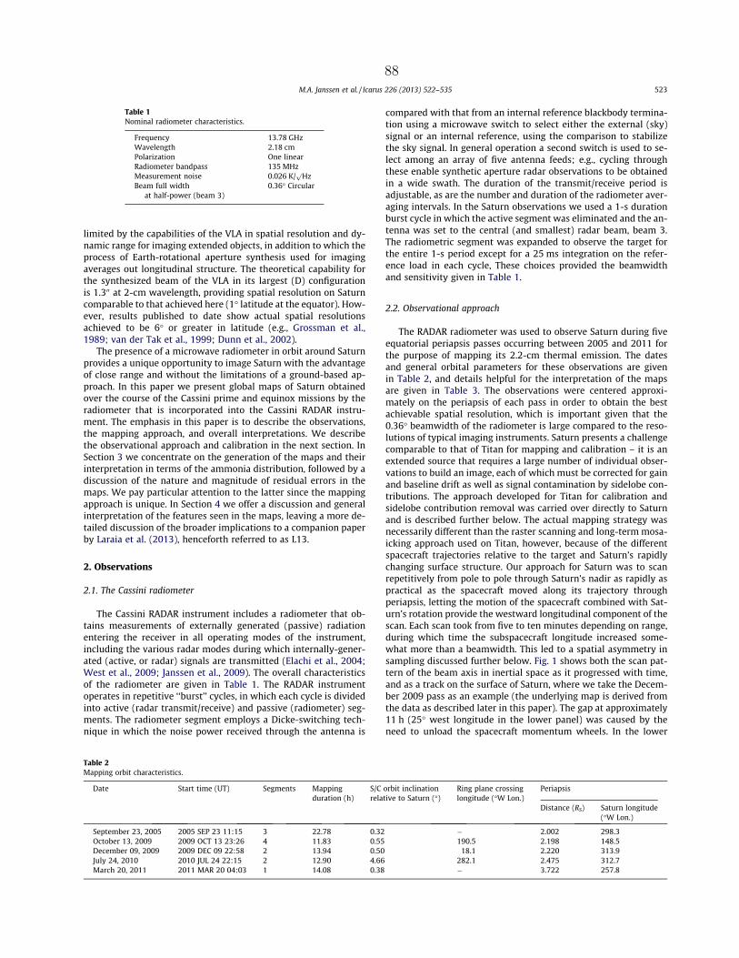
limited by the capabilities of the VLA in spatial resolution and dy-namic range for imaging extended objects, in addition to which theprocess of Earth-rotational aperture synthesis used for imagingaverages out longitudinal structure. The theoretical capability forthe synthesized beam of the VLA in its largest (D) configurationis 1.300 at 2-cm wavelength, providing spatial resolution on Saturncomparable to that achieved here (1 latitude at the equator). How-ever, results published to date show actual spatial resolutionsachieved to be 6 or greater in latitude (e.g., Grossman et al.,1989; van der Tak et al., 1999; Dunn et al., 2002).

The presence of a microwave radiometer in orbit around Saturnprovides a unique opportunity to image Saturn with the advantageof close range and without the limitations of a ground-based ap-proach. In this paper we present global maps of Saturn obtainedover the course of the Cassini prime and equinox missions by theradiometer that is incorporated into the Cassini RADAR instru-ment. The emphasis in this paper is to describe the observations,the mapping approach, and overall interpretations. We describethe observational approach and calibration in the next section. InSection 3 we concentrate on the generation of the maps and theirinterpretation in terms of the ammonia distribution, followed by adiscussion of the nature and magnitude of residual errors in themaps. We pay particular attention to the latter since the mappingapproach is unique. In Section 4 we offer a discussion and generalinterpretation of the features seen in the maps, leaving a more de-tailed discussion of the broader implications to a companion paperby Laraia et al. (2013), henceforth referred to as L13.

2. Observations

2.1. The Cassini radiometer

The Cassini RADAR instrument includes a radiometer that ob-tains measurements of externally generated (passive) radiationentering the receiver in all operating modes of the instrument,including the various radar modes during which internally-gener-ated (active, or radar) signals are transmitted (Elachi et al., 2004;West et al., 2009; Janssen et al., 2009). The overall characteristicsof the radiometer are given in Table 1. The RADAR instrumentoperates in repetitive ‘‘burst’’ cycles, in which each cycle is dividedinto active (radar transmit/receive) and passive (radiometer) seg-ments. The radiometer segment employs a Dicke-switching tech-nique in which the noise power received through the antenna is

compared with that from an internal reference blackbody termina-tion using a microwave switch to select either the external (sky)signal or an internal reference, using the comparison to stabilizethe sky signal. In general operation a second switch is used to se-lect among an array of five antenna feeds; e.g., cycling throughthese enable synthetic aperture radar observations to be obtainedin a wide swath. The duration of the transmit/receive period isadjustable, as are the number and duration of the radiometer aver-aging intervals. In the Saturn observations we used a 1-s durationburst cycle in which the active segment was eliminated and the an-tenna was set to the central (and smallest) radar beam, beam 3.The radiometric segment was expanded to observe the target forthe entire 1-s period except for a 25 ms integration on the refer-ence load in each cycle, These choices provided the beamwidthand sensitivity given in Table 1.

2.2. Observational approach

The RADAR radiometer was used to observe Saturn during fiveequatorial periapsis passes occurring between 2005 and 2011 forthe purpose of mapping its 2.2-cm thermal emission. The datesand general orbital parameters for these observations are givenin Table 2, and details helpful for the interpretation of the mapsare given in Table 3. The observations were centered approxi-mately on the periapsis of each pass in order to obtain the bestachievable spatial resolution, which is important given that the0.36 beamwidth of the radiometer is large compared to the reso-lutions of typical imaging instruments. Saturn presents a challengecomparable to that of Titan for mapping and calibration – it is anextended source that requires a large number of individual obser-vations to build an image, each of which must be corrected for gainand baseline drift as well as signal contamination by sidelobe con-tributions. The approach developed for Titan for calibration andsidelobe contribution removal was carried over directly to Saturnand is described further below. The actual mapping strategy wasnecessarily different than the raster scanning and long-term mosa-icking approach used on Titan, however, because of the differentspacecraft trajectories relative to the target and Saturn’s rapidlychanging surface structure. Our approach for Saturn was to scanrepetitively from pole to pole through Saturn’s nadir as rapidly aspractical as the spacecraft moved along its trajectory throughperiapsis, letting the motion of the spacecraft combined with Sat-urn’s rotation provide the westward longitudinal component of thescan. Each scan took from five to ten minutes depending on range,during which time the subspacecraft longitude increased some-what more than a beamwidth. This led to a spatial asymmetry insampling discussed further below. Fig. 1 shows both the scan pat-tern of the beam axis in inertial space as it progressed with time,and as a track on the surface of Saturn, where we take the Decem-ber 2009 pass as an example (the underlying map is derived fromthe data as described later in this paper). The gap at approximately11 h (25 west longitude in the lower panel) was caused by theneed to unload the spacecraft momentum wheels. In the lower

Table 1Nominal radiometer characteristics.

Frequency 13.78 GHzWavelength 2.18 cmPolarization One linearRadiometer bandpass 135 MHzMeasurement noise 0.026 K/

pHz

Beam full widthat half-power (beam 3)

0.36 Circular

Table 2Mapping orbit characteristics.

Date Start time (UT) Segments Mappingduration (h)

S/C orbit inclinationrelative to Saturn ()

Ring plane crossinglongitude (W Lon.)

Periapsis

Distance (RS) Saturn longitude(W Lon.)

September 23, 2005 2005 SEP 23 11:15 3 22.78 0.32 2.002 298.3October 13, 2009 2009 OCT 13 23:26 4 11.83 0.55 190.5 2.198 148.5December 09, 2009 2009 DEC 09 22:58 2 13.94 0.50 18.1 2.220 313.9July 24, 2010 2010 JUL 24 22:15 2 12.90 4.66 282.1 2.475 312.7March 20, 2011 2011 MAR 20 04:03 1 14.08 0.38 3.722 257.8

M.A. Janssen et al. / Icarus 226 (2013) 522–535 523

88

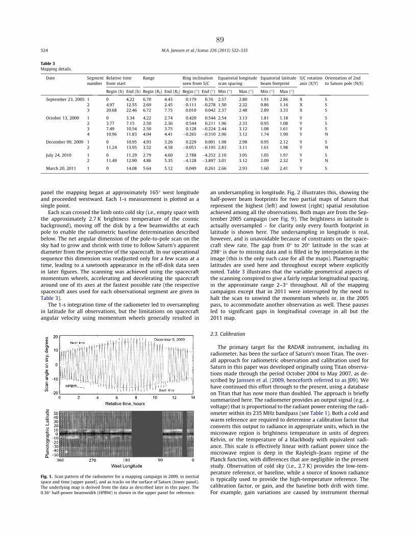
panel the mapping began at approximately 165 west longitudeand proceeded westward. Each 1-s measurement is plotted as asingle point.

Each scan crossed the limb onto cold sky (i.e., empty space withthe approximately 2.7 K brightness temperature of the cosmicbackground), moving off the disk by a few beamwidths at eachpole to enable the radiometric baseline determination describedbelow. The net angular dimension of the pole-to-pole scan on thesky had to grow and shrink with time to follow Saturn’s apparentdiameter from the perspective of the spacecraft. In our operationalsequence this dimension was readjusted only for a few scans at atime, leading to a sawtooth appearance in the off-disk data seenin later figures. The scanning was achieved using the spacecraftmomentum wheels, accelerating and decelerating the spacecraftaround one of its axes at the fastest possible rate (the respectivespacecraft axes used for each observational segment are given inTable 3).

The 1-s integration time of the radiometer led to oversamplingin latitude for all observations, but the limitations on spacecraftangular velocity using momentum wheels generally resulted in

an undersampling in longitude. Fig. 2 illustrates this, showing thehalf-power beam footprints for two partial maps of Saturn thatrepresent the highest (left) and lowest (right) spatial resolutionachieved among all the observations. Both maps are from the Sep-tember 2005 campaign (see Fig. 9). The brightness in latitude isactually oversampled – for clarity only every fourth footprint inlatitude is shown here. The undersampling in longitude is real,however, and is unavoidable because of constraints on the space-craft slew rate. The gap from 0 to 20 latitude in the scan at298 is due to missing data and is filled in by interpolation in theimage (this is the only such case for all the maps). Planetographiclatitudes are used here and throughout except where explicitlynoted. Table 3 illustrates that the variable geometrical aspects ofthe scanning conspired to give a fairly regular longitudinal spacing,in the approximate range 2–3 throughout. All of the mappingcampaigns except that in 2011 were interrupted by the need tohalt the scan to unwind the momentum wheels or, in the 2005pass, to accommodate another observation as well. These pausesled to significant gaps in longitudinal coverage in all but the2011 map.

2.3. Calibration

The primary target for the RADAR instrument, including itsradiometer, has been the surface of Saturn’s moon Titan. The over-all approach for radiometric observation and calibration used forSaturn in this paper was developed originally using Titan observa-tions made through the period October 2004 to May 2007, as de-scribed by Janssen et al. (2009, henceforth referred to as J09). Wehave continued this effort through to the present, using a databaseon Titan that has now more than doubled. The approach is brieflysummarized here. The radiometer provides an output signal (e.g., avoltage) that is proportional to the radiant power entering the radi-ometer within its 235 MHz bandpass (see Table 1). Both a cold andwarm reference are required to determine a calibration factor thatconverts this output to radiance in appropriate units, which in themicrowave region is brightness temperature in units of degreesKelvin, or the temperature of a blackbody with equivalent radi-ance. This scale is effectively linear with radiant power since themicrowave region is deep in the Rayleigh–Jeans regime of thePlanck function, with differences that are negligible in the presentstudy. Observation of cold sky (i.e., 2.7 K) provides the low-tem-perature reference, or baseline, while a source of known radianceis typically used to provide the high-temperature reference. Thecalibration factor, or gain, and the baseline both drift with time.For example, gain variations are caused by instrument thermal

Table 3Mapping details.

Date Segmentnumber

Relative timefrom start

Range Ring inclinationseen from S/C

Equatorial longitudescan spacing

Equatorial latitudebeam footprint

S/C rotationaxis (X/Y)

Orientation of 2ndto Saturn pole (N/S)

Begin (h) End (h) Begin (RS) End (RS) Begin () End () Min () Max () Min () Max ()

September 23, 2005 1 0 4.22 6.70 4.43 0.179 0.76 2.57 2.80 1.91 2.86 X S2 4.97 12.55 2.69 2.45 0.111 0.278 1.50 2.32 0.86 1.16 X S3 20.68 22.46 6.72 7.75 0.010 0.042 2.37 2.48 2.89 3.33 X S

October 13, 2009 1 0 3.34 4.22 2.74 0.420 0.544 2.54 3.13 1.81 1.18 Y S2 3.77 7.15 2.50 2.36 0.544 0.211 1.96 2.33 0.95 1.08 Y S3 7.49 10.54 2.50 3.75 0.128 0.224 2.44 3.12 1.08 1.61 Y S4 10.96 11.83 4.04 4.41 0.265 0.310 2.96 3.12 1.74 1.90 Y N

December 09, 2009 1 0 10.95 4.93 3.26 0.229 0.001 1.98 2.98 0.95 2.12 Y S2 11.24 13.95 3.52 4.58 0.051 0.195 2.83 3.11 1.61 1.98 Y N

July 24, 2010 1 0 11.29 2.79 4.60 2.788 4.252 2.10 3.05 1.05 1.97 Y S2 11.49 12.90 4.86 5.35 4.128 3.897 3.01 3.12 2.09 2.32 Y N

March 20, 2011 1 0 14.08 5.64 5.12 0.049 0.261 2.66 2.93 1.60 2.41 Y S

Fig. 1. Scan pattern of the radiometer for a mapping campaign in 2009, in inertialspace and time (upper panel), and as tracks on the surface of Saturn (lower panel).The underlying map is derived from the data as described later in this paper. The0.36 half-power beamwidth (HPBW) is shown in the upper panel for reference.

524 M.A. Janssen et al. / Icarus 226 (2013) 522–535

89

variations resulting from instrument warm up after turn on as wellas variations in the observing geometry and consequent solar illu-mination of the instrument during the course of the observations.Such variations also affect the baseline. Observations of cold skyobtained by moving off source from time to time enable the base-line drift to be tracked, while frequent views of our internal refer-ence load allows relative gain variations to be tracked.

The absolute calibration, or the conversion of output voltage toradiometric brightness temperature in units of degrees Kelvin,must be independently obtained, and we used Titan for this pur-pose. During the period covered by J09, Titan was observed bythe RADAR radiometer in 69 individual observing segments during18 flybys of Titan by the Cassini spacecraft, at a variety of geome-tries and polarizations covering most of Titan, and at distancesranging from 1000 to 100,000 km. Global map mosaics of effectivedielectric constant were determined from the measured thermalpolarization. These enabled the construction of global maps ofequivalent brightness temperature at normal incidence. Weshowed that the emissivity could be reliably predicted to betterthan 1% in special regions such as the dune fields and methaneseas, which allowed us to make an absolute calibration of thebrightness based on the measured physical temperature of the sur-face from the Huygens lander (93.7 K, Fulchignoni et al., 2005). Inaddition to the increased database of Titan observations, our phys-ical reference temperature is now supplemented by extensive

infrared surface temperature measurements by the Cassini Com-posite Infrared Spectrometer (CIRS, Jennings et al., 2009; Cottiniet al., 2012), which we used to develop a seasonal surface temper-ature model for Titan’s entire surface. This work will be reported ina future paper; however, we note here that the net calibration scalechange from the J09 paper amounted to only about 0.5%.

Knowledge of the beam pattern is essential to construct abso-lute maps from the observations. The pattern of the circular centralbeam has been measured by scanning the Sun’s emission to anaccuracy of one part in 104 out to 2 from the boresight as de-scribed in J09. However, the sidelobes out to as far as 60 areresponsible for a large additional signal, particularly at close rangewhere the disk of Titan fills a significant fraction of the forwardhemisphere; e.g., at close range the contribution of sidelobes out-side 2 amount to nearly 30% of the main beam signal! These side-lobes were never measured in the ground calibrations and wereunknown before the Titan observations; however, we solved forthem as a byproduct of the mapping. Their knowledge allowedus to compute and remove this error signal for all Titan observa-tions to within better than 1% of the main beam signal. Our solu-tion was used for Saturn, which presents the same problem.

Finally, we consider that the gain of the radiometer may changein the long term over time, as for example might be expected dueto aging of receiver components. Hence we included the determi-nation of a slow linear drift of the gain in the Titan calibration overyears. Although Titan was the reference used for this in the J09 cal-ibration, we found that it was better determined from the presentSaturn observations themselves. These considerations along withdetailed error estimates are discussed following the presentationof the maps in the next section.

3. Mapping Saturn

3.1. Emission model

The results presented in this paper are given as maps of bright-ness temperature relative to brightness temperatures computedfor an assumed model for Saturn’s structure and ammonia distri-bution. The radiative transfer calculations used for this comparisonrely on a computer program currently under development for theJuno Microwave Radiometer (MWR) experiment at Jupiter (Janssenet al., 2005, in preparation). This program, called the Juno Atmo-spheric Microwave Radiative Transfer (JAMRT) program, constructsmodel atmospheres and carries out radiative transfer calculationsat microwave frequencies. This program was written specificallyto support the Juno mission to Jupiter, but it is equally useful forthe analysis of the Saturn observations reported here when thephysical parameters and composition appropriate for Saturn aresubstituted for those of Jupiter.

The model atmosphere part of the JAMRT program builds deepconvective models, including dry adiabatic lapse rates in the deepatmosphere and wet adiabatic lapse rates in the cloud formingregions. The release of heat in the ortho–para transition of H2,assumed to be in equilibrium in all levels, is included. The gravita-tional potential is calculated using the equation for the potentialfunction for a fluid having a uniform angular velocity (i.e., Lindalet al., 1985). We use the JPL NASA web site (ssd.jpl.nasa.gov/?grav-ity_fields_op) to obtain the gravity field data. The gravitationalmoments are referred to the distance 60,330 km. The radius ofSaturn is taken to be 60,268 km. We use a rotation period of 10 h32 m 35 s. The mass of Saturn in units of GM is taken to be37,931,208 km3/s2. For the purposes of the radiative transfer calcu-lations, we assume the atmosphere be stratified with the normal tothe stratified layers following the normal to the equipotential sur-faces of Saturn. The reference surface is located at the 1-bar

Fig. 2. Beam footprints on Saturn at two extremes of resolution. Shown are the half-power beam footprints on two partial maps of Saturn from September 2005.

M.A. Janssen et al. / Icarus 226 (2013) 522–535 525

90

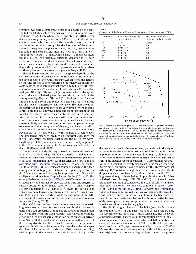
pressure level with a temperature that is selectable by the user.The full model atmosphere extends over the pressure range from1000 bars to 550 mb where the temperature is 110 K. Layerthicknesses are generally taken to be 100 m except in the vicinityof cloud layers, where we reduce the layer thickness to accountfor the transition that accompanies the formation of the clouds.The dry atmosphere components are H2, He, CH4, and the noblegas Argon. The condensable gases are H2O, H2S, PH3 and NH3.The condensates are H2O ice, H2O liquid, NH3/H2O solution, NH4SHice, and NH3 ice. The program calculates the depletion of NH3 bothin the water cloud region, due to its absorption into water droplets,and in the ammonium hydrosulfide cloud region due to its interac-tion with H2S to form NH4SH. Vapor pressures and moist adiabatsfor these gases and condensates are given in Atreya (1986).

The brightness temperature of the atmosphere depends on thedistribution of microwave absorbers with temperature. Central tothe development of the JAMRT program was an effort, also fundedby the Juno project, to better determine the microwave absorptioncoefficients of the constituents that contribute to Jupiter’s thermalmicrowave emission. The potential absorbers include (1) the polar-ized gases NH3, H2O, PH3, and H2S, (2) pressure-induced absorptiondue to the non-polarized gases that constitute the bulk of theatmosphere, H2, He, and CH4, and (3) cloud particles. Gaseousammonia, as the dominant source of microwave opacity in thegas giant planet atmospheres, has been given the most attention.Its absorption is due primarily to its very strong inversion bandcentered around 1.4-cm wavelength, and its absorption at longerwavelengths can be modeled as due to the pressure-broadenedwings of the lines in this band along with some contribution frominfrared rotational transitions. Its absorption coefficient has beenmeasured in H2–He mixtures over a pressure–temperature rangeconsistent with the atmospheres of the gas giant planets, up to lim-iting values of 100 bars and 500 K respectively (Hanley et al., 2009;Deveraj, 2011). The data were fit with the help of a Ben-Reuvenline-broadening model to produce an empirical expression forthe NH3 absorption coefficient that covers the 1.3–50-cm wave-length range of the Juno experiment. The uncertainty applicableto the 2.2-cm wavelength range for Saturn is estimated to be betterthan 10% (Hanley et al., 2009).

Our absorption model for PH3 is based on pressure-broadenedrotational transitions using a Van Vleck–Weisskopf lineshape, withabsorption consistent with laboratory measurements (Hoffmanet al., 2001; Mohammed, 2004). A similar calculation for H2S is alsoconsistent with laboratory measurements (DeBoer and Steffes,1994). Although H2O is a significant source of opacity in the deepatmosphere, it is largely absent from the region responsible forthe 2.2-cm emission and of negligible importance here. Our modelfor H2O absorption is from Karpowicz and Steffes (2011a, 2011b).Other polarized molecules (e.g., HCN, CN, and CO) are of much low-er abundance and are not considered. Cloud NH3 and NH4SH iceparticle absorption is estimated based on an assumed complexdielectric constant of 4.5 + 3.25 106m (GHz) for particle size2.2 cm, a value based on data taken at 1 MHz on NH3 ice by Lor-enz (1998) and highly uncertain, while the absorption of H2O/NH3

mixtures in the water cloud region are based on laboratory mea-surements (Duong, 2011).

The JAMRT program has the capability to compute radiometricbrightness temperatures for user-selectable absorber concentra-tions and cloud properties of condensable species, including theirrelative humidities in the cloud regions. Table 4 gives an estimateof Saturn’s deep atmosphere composition based on values derivedfrom Atreya (2010). Fig. 3 shows the absorption with pressure ofthe leading absorbers in the atmosphere computed for an atmo-sphere with this composition, assuming that all condensable spe-cies form fully saturated clouds (i.e., 100% relative humidity)with no precipitation. Gaseous ammonia is seen to be by far the

dominant absorber in the atmosphere, particularly in the regionresponsible for the 2.2-cm emission. Phosphine is the next mostimportant absorber above the water cloud region, although witha contribution three or four orders of magnitude less than that ofNH3 in the effective region of emission. H2S absorption is yet smal-ler, besides which it effectively disappears in the region where the2.2-cm emission originates as it combines with NH3. We note thatalthough H2S contributes negligibly to the absorption directly, itsdeep abundance can have a significant impact on the 2.2-cmbrightness through this depletion of upper-level ammonia. Otherpolarized molecules (e.g., HCN, CN, and CO) are of much lowerabundance and are not considered. The sum of collision-inducedabsorption due to H2, He, and CH4 collisions is shown (Ortonet al., 2007; Birnbaum et al., 1996; Borysow and Frommhold,1986) and seen to be negligible at our wavelength. The contribu-tions from NH3 and NH4SH ice particle shown in the figure are rea-sonable but rough estimates, but are highly conservative becauseof the assumption that no precipitation occurs. We consider theirpossible contributions to be negligible.

The JAMRT program has much flexibility (see L13 for a moregeneral application). In this paper, we take as our standard onlythe very simple case illustrated in Fig. 4, which assumes the modelatmosphere described above with the composition given in Table 4,moist adiabatic temperature lapse rates and full saturation forcloud regions, and a temperature of 134.8 K at the 1-bar pressurelevel based on the Voyager measurement by Lindal et al. (1985).We use this case as a reference model with which to compareour brightness measurements. Fig. 4 depicts the atmosphere’s

Table 4Composition of the Saturn reference model atmosphere (based on Atreya (2010)).

Constituent Solar abundance (mixingratio relative to H2)

Enrichment of the Saturnatmosphere relative to solar

He 0.195 0.6955CH4 5.5 104 9.4H2O 1.026 103 3.0NH3 1.352 104 3.0H2S 3.10 105 5.0Ar 7.24 106 1.0PH3 5.14 107 7.5

Fig. 3. Microwave absorption profiles at 2-cm wavelength for possible absorbingconstituents through the NH3 cloud region. The atmospheric composition is that ofour reference model as given in Table 4. The dotted lines indicate conservativeestimates for various particulate absorbers as indicated, while the other linesrepresent individual gases identified in the legend. The curve labeled CIA includesthe sum of H2H2, H2He, and H2CH4 collision-induced absorption.

526 M.A. Janssen et al. / Icarus 226 (2013) 522–535

91

pressure–temperature relationship along with the ammonia distri-bution and the corresponding weighting function at 2.2 cm. Notethat the ammonia mixing ratio is not constant beneath its nominalsaturation level – this is because it is assumed to interact with sub-cloud H2S to form ammonium hydrosulfide, which reduces the NH3

mixing ratio until all of the sulfur is depleted (the loss of NH3 intowater cloud drops is small relative to this). For example, the micro-wave spectrum has been interpreted to show such a subclouddepletion (Briggs and Sackett, 1989; Grossman, 1990; de Pateret al., 2001). The ammonia concentration above the saturation levelis assumed to follow the Clausius–Clapeyron equation, equivalentto the assumption that the cloud region relative humidity is every-where 100%.

All results in the following are presented as residuals after thesubtraction of the reference model brightness values from themeasured values, where we take into account both emission angleand latitude dependence in the model for each measurement point.Unless supersaturation is allowed, any plausible redistribution ofammonia in this model for a given deep abundance can only re-duce the amount of vapor in the emission region, which lowersthe weighting function and results in a higher brightness temper-ature because of the atmospheric temperature lapse rate. Hencethe brightness temperature residuals are expected to all be posi-tive. Since the 2-cm weighting function lies almost entirely withinthe saturation region in the reference model, the computed bright-ness temperatures are only weakly dependent on the deep abun-dance of ammonia. Further, the brightness temperature isinsensitive to physical temperature variations in the cloud region.If the specific humidity were held constant, then the brightnesstemperature would indeed vary directly with the kinetic tempera-ture; however, at constant relative humidity as assumed in themodel, the weighting function follows the ammonia as the temper-ature of the cloud-region atmosphere is varied and tends to stay

constant in relation to temperature. There is a small effect, about1 K of brightness temperature change for a 5 K shift in the adiabat,caused by the corresponding pressure shift with temperature andthe effect of this on the absorption model. In view of these consid-erations we conclude that the radiometric brightness at 2.2 cm de-pends to first order only on the ammonia distribution, and inparticular only on the cloud-level humidity for small departuresfrom the reference model. However, when the cloud-level ammo-nia becomes highly depleted, the weighting function descends intothe subcloud region and the interpretation becomes more compli-cated. This condition occurs in several important regions in thepresent maps, and L13 presents a more complete discussion ofthe implications that the 2.2-cm data hold for the ammonia sub-cloud distribution in such a case.

3.2. Generating maps

The time-ordered scan data consist of a stream of relative val-ues for the antenna temperatures on the sky and the reference loadobtained each second. Maps were produced from these data in aseries of steps, which we outline here and illustrate below. To be-gin, we note that we use the same convention as described in J09for defining the power collected by the antenna, the ‘‘antenna tem-perature’’, and the source brightness, or ‘‘brightness temperature’’.In usual practice the antenna temperature, or radiant power col-lected by the antenna, is the brightness temperature integratedover the whole sky as weighted by a normalized antenna gain pat-tern; e.g., the antenna temperature of a blackbody distribution overthe whole sphere would be the blackbody brightness temperature(cf. Janssen, 1993). In principle the brightness temperature distri-bution may be determined from measured antenna temperaturesby inverting this relationship, subject to a loss of spatial resolutionat scales smaller than the main antenna beam. However, we as-sume here an antenna temperature calibration scale that is nor-malized over only the measured antenna pattern inside a cutoffangle of 2 where the pattern is well known (see Section 2.2 ofJ09), with a gain calibration factor applied to the raw radiometersignal as appropriately determined for this convention. It remainsthen to determine and subtract the sidelobe contributions, afterwhich the correctly scaled brightness distribution is obtained withknowledge of this truncated main beam pattern (henceforth calledthe TMB). This approach is convenient for the case where the abso-lute calibration of measurements over an extended source is basedon source ‘‘ground truth’’, as was the case for Titan, since residualerrors in the knowledge of both the near and far beam pattern arecanceled out to first order. For example, the net results were shownin J09 to be insensitive to the exact choice of cutoff angle.

The gain calibration determined for Titan was first directly ap-plied to the raw data on Saturn to convert them to the Kelvin scalewithout concern for baseline variations, using the above conven-tion for beam normalization. At the same time, the beam patternwas convolved with the brightness temperature distribution ofour reference model for the observing geometry of each measure-ment point to produce a set of model antenna temperatures. Aswith Titan, the beam pattern convolution was performed sepa-rately for the TMB and the far sidelobe pattern (FSL in the follow-ing). This convolution took into account the modeled emission-angle variation of the brightness across Saturn and assumed a va-lue of 2.7 K for points off the disk. The model included a simpledescription of the ring blockage for the FSL convolution, but notfor the TMB convolution for reasons discussed later. The cold skybaseline was determined from the excursions off the disk at theend of every scan, using the sum of the TMB and FSL convolutionsto correct the baseline for all sidelobe contributions to the off-diskmeasurements. Specifically, each off-disk excursion was used toestimate a baseline correction to the calibrated data set applicable

Fig. 4. Atmospheric model used to compute reference brightness temperatures. Thetemperature (dotted line) and NH3 mixing ratio in units of solar abundance (thicksolid line) are shown as a function of pressure and altitude in the vicinity of theammonia cloud region in the atmosphere. The reference model assumes 100%relative humidity for ammonia above its saturation level, while the light solid lineshows a case for 50% relative humidity. The decrease in NH3 mixing ratio above the5-bar level is due to reaction with H2S to form NH4SH ice. The dashed line shows the2.2-cm wavelength weighting function in arbitrary linear units at normal incidencefor the reference model.

M.A. Janssen et al. / Icarus 226 (2013) 522–535 527

92

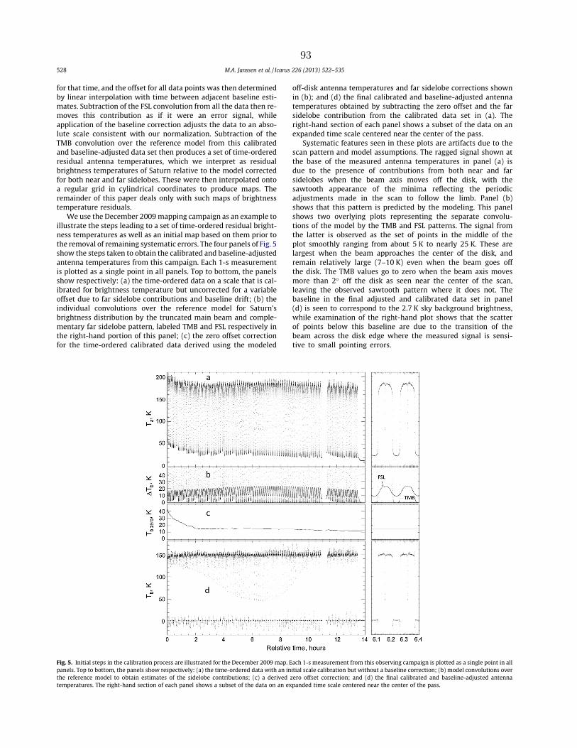
for that time, and the offset for all data points was then determinedby linear interpolation with time between adjacent baseline esti-mates. Subtraction of the FSL convolution from all the data then re-moves this contribution as if it were an error signal, whileapplication of the baseline correction adjusts the data to an abso-lute scale consistent with our normalization. Subtraction of theTMB convolution over the reference model from this calibratedand baseline-adjusted data set then produces a set of time-orderedresidual antenna temperatures, which we interpret as residualbrightness temperatures of Saturn relative to the model correctedfor both near and far sidelobes. These were then interpolated ontoa regular grid in cylindrical coordinates to produce maps. Theremainder of this paper deals only with such maps of brightnesstemperature residuals.

We use the December 2009 mapping campaign as an example toillustrate the steps leading to a set of time-ordered residual bright-ness temperatures as well as an initial map based on them prior tothe removal of remaining systematic errors. The four panels of Fig. 5show the steps taken to obtain the calibrated and baseline-adjustedantenna temperatures from this campaign. Each 1-s measurementis plotted as a single point in all panels. Top to bottom, the panelsshow respectively: (a) the time-ordered data on a scale that is cal-ibrated for brightness temperature but uncorrected for a variableoffset due to far sidelobe contributions and baseline drift; (b) theindividual convolutions over the reference model for Saturn’sbrightness distribution by the truncated main beam and comple-mentary far sidelobe pattern, labeled TMB and FSL respectively inthe right-hand portion of this panel; (c) the zero offset correctionfor the time-ordered calibrated data derived using the modeled

off-disk antenna temperatures and far sidelobe corrections shownin (b); and (d) the final calibrated and baseline-adjusted antennatemperatures obtained by subtracting the zero offset and the farsidelobe contribution from the calibrated data set in (a). Theright-hand section of each panel shows a subset of the data on anexpanded time scale centered near the center of the pass.

Systematic features seen in these plots are artifacts due to thescan pattern and model assumptions. The ragged signal shown atthe base of the measured antenna temperatures in panel (a) isdue to the presence of contributions from both near and farsidelobes when the beam axis moves off the disk, with thesawtooth appearance of the minima reflecting the periodicadjustments made in the scan to follow the limb. Panel (b)shows that this pattern is predicted by the modeling. This panelshows two overlying plots representing the separate convolu-tions of the model by the TMB and FSL patterns. The signal fromthe latter is observed as the set of points in the middle of theplot smoothly ranging from about 5 K to nearly 25 K. These arelargest when the beam approaches the center of the disk, andremain relatively large (7–10 K) even when the beam goes offthe disk. The TMB values go to zero when the beam axis movesmore than 2 off the disk as seen near the center of the scan,leaving the observed sawtooth pattern where it does not. Thebaseline in the final adjusted and calibrated data set in panel(d) is seen to correspond to the 2.7 K sky background brightness,while examination of the right-hand plot shows that the scatterof points below this baseline are due to the transition of thebeam across the disk edge where the measured signal is sensi-tive to small pointing errors.

Fig. 5. Initial steps in the calibration process are illustrated for the December 2009 map. Each 1-s measurement from this observing campaign is plotted as a single point in allpanels. Top to bottom, the panels show respectively: (a) the time-ordered data with an initial scale calibration but without a baseline correction; (b) model convolutions overthe reference model to obtain estimates of the sidelobe contributions; (c) a derived zero offset correction; and (d) the final calibrated and baseline-adjusted antennatemperatures. The right-hand section of each panel shows a subset of the data on an expanded time scale centered near the center of the pass.

528 M.A. Janssen et al. / Icarus 226 (2013) 522–535

93

The brightness residuals were then used to generate the globalcylindrical map shown in Fig. 6. This map was made using the idlTRIANGULATE procedure and TRIGRID function to interpolate theirregularly-spaced time-ordered measurements onto a regular gridwith 0.5 spacing, using idl’s CONTOUR plotting routine to producethe map. The gray scale was chosen to show the unmeasured por-tion of the plot as a dark gray corresponding to a residual of 0 K,i.e., as the brightness of the reference model, compared to whichthe maps points are expected to show a lighter shade. The black re-gion along the equator is due to blockage by the rings, which aremostly optically thick and of much lower brightness than the disk.This and all following maps were cut off beyond an emission angleof 70, where small errors in pointing begin to dominate thebrightness uncertainty.

This map demonstrates the ability of the radiometer to distin-guish among small features with brightness variations approach-ing the 0.1 K white-noise level of the measurements, a capabilityalso demonstrated in the Titan observations. Nevertheless themap contains artifacts with greater brightness variations on largespatial scales that need to be accounted for. The most obvious oc-curs at the start of the scan at approximately 165 west longitude,where the first 30 or so of the map westward from this appearssignificantly cooler than the remainder of the map. This is an arti-fact seen only in the December 2009 map. In all other observationswe used a warm-up period of 3 h prior to operations to allow theradiometer to thermally stabilize; however, in this case we wereprevented from doing this by a power conflict with a previous(non-RADAR) observation. We elected to start our mapping imme-diately at RADAR turn-on knowing that our calibration algorithmwas not valid for the resulting thermal transient. We in fact seeabout a 3 K brightness temperature drift in the map, a warm-up ef-fect also apparent in the baseline drift seen in panel (c) of Fig. 5.Another apparent artifact is a striping with longitude, a smallersystematic effect that we ascribe to the incomplete removal ofsidelobe signal in the establishment of the baseline.

An artifact not immediately apparent but also important to con-sider is a low-spatial-frequency brightness error caused by range-related errors in removing the far sidelobe contribution. The solu-tion for the Titan mapping was less dependent on the removal ofthis error signal because of the way the map mosaic was con-structed. The Titan mapping used low-resolution observationsmade at long range, with small and ultimately accountable farsidelobe contributions, to provide the absolute map level, whileobservations at closer range were used to provide the higher spa-tial resolution components. At the same time the far sidelobe con-tributions were determined from the range-dependent offsetsobtained in reconciling near and far-range measurements of thesame regions on Titan. The sidelobe pattern was retrieved as partof this reconciliation, for example. This was simplified by assumingit to depend only on polar angle, i.e., to be uniform in azimuth. Thisprocess essentially filtered out residual errors associated with the

large sidelobe contributions from the close-range measurements,and so was adequate for Titan. This solution left the possibility ofresidual low-spatial-frequency errors for the Saturn mapping,however, and are estimated based on the J09 analysis to be presentat around the 1% level.

We searched for such residual sidelobe contamination in themaps, anticipating that they would appear as systematic errorsthat depend on spacecraft range and orientation. We took advan-tage of regions of latitude in both hemispheres in which there is lit-tle or no longitudinal structure; in particular, we considered thebands from about 15 to 55 latitude in the north, and 15 to32 latitude in the south, where no longitudinal structure was dis-cernable in any of the maps except for the northern storm in the2011 map and the ring blockage in the 2010 map. Excluding thelatter, we expected the average brightness across these latitudesto be approximately the same for each scan. Fig. 7 shows theweighted average of these ‘‘quiescent’’ bands in both hemispheresplotted for each scan as a function of elapsed time, with the meanfor all scans subtracted to give a zero mean offset. The features inthese plots can be associated with the three main sources of errorwe expect to see. First, the general trend among the plots followsthe shape of the respective range curves, which are also plottedand shown as solid lines. This trend indicates an uncorrectedsidelobe contribution that varies by as much as 1 K with range,consistent with the 1% sidelobe error residual anticipated. Sec-ondly, gain drifts are present, most notably the 2% drift seen atthe start of the December 2009 mapping campaign. Another possi-ble gain variation is apparent in the third segment of the Septem-ber 2005 campaign, which is offset by about 1% relative to theaverage over the same range in the first segment. Thirdly, theremaining scatter may be explained by errors in the baseline cor-rection, caused by a combination of short-term gain drifts andresidual errors in the offset modeling. The latter explanation isconsistent with the correlation between the patterns in these andthe TMB modeling of the off-limb scans in panel (b) of Fig. 5; e.g.,compare the upward drift seen in Fig. 7 for the December 2009 plotfrom about 11 to 12 h to the minima at the same times in the TMBvalues in panel (b) of Fig. 5.

We also used the quiescent band mean brightness for each mapto examine the long-term dependence on gain (or Saturn’s meanbrightness) with time. The original Titan calibration used a seriesof measurements of Titan’s unresolved disk brightness tempera-ture made from long range to search for gain calibration drift inthe measurements (J09). This was reexamined with distant Titanobservations obtained through 2012, finding a downward gaindrift of 0.2% per year, but barely statistically significant. This ratewas incorporated into the present Saturn calibration. Fig. 8 showsthe dependence with time on the quiescent band mean brightness-es obtained using this gain drift rate. If correct, this would indicatea steady brightness temperature decrease of Saturn in these quies-cent bands, which we consider unlikely. Rather, we take the drift

Fig. 6. Global map of brightness temperature residuals from December 2009, before further adjustment to remove artifacts.

M.A. Janssen et al. / Icarus 226 (2013) 522–535 529

94

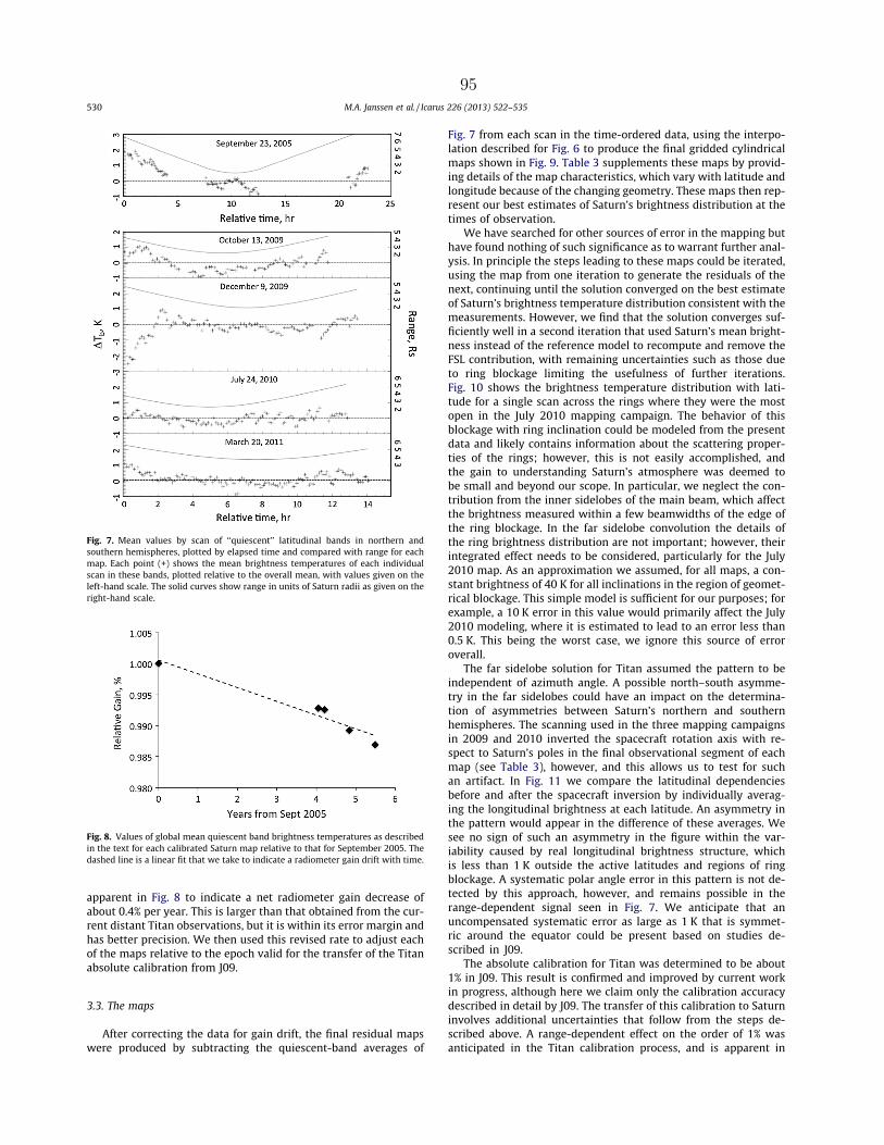
apparent in Fig. 8 to indicate a net radiometer gain decrease ofabout 0.4% per year. This is larger than that obtained from the cur-rent distant Titan observations, but it is within its error margin andhas better precision. We then used this revised rate to adjust eachof the maps relative to the epoch valid for the transfer of the Titanabsolute calibration from J09.

3.3. The maps

After correcting the data for gain drift, the final residual mapswere produced by subtracting the quiescent-band averages of

Fig. 7 from each scan in the time-ordered data, using the interpo-lation described for Fig. 6 to produce the final gridded cylindricalmaps shown in Fig. 9. Table 3 supplements these maps by provid-ing details of the map characteristics, which vary with latitude andlongitude because of the changing geometry. These maps then rep-resent our best estimates of Saturn’s brightness distribution at thetimes of observation.

We have searched for other sources of error in the mapping buthave found nothing of such significance as to warrant further anal-ysis. In principle the steps leading to these maps could be iterated,using the map from one iteration to generate the residuals of thenext, continuing until the solution converged on the best estimateof Saturn’s brightness temperature distribution consistent with themeasurements. However, we find that the solution converges suf-ficiently well in a second iteration that used Saturn’s mean bright-ness instead of the reference model to recompute and remove theFSL contribution, with remaining uncertainties such as those dueto ring blockage limiting the usefulness of further iterations.Fig. 10 shows the brightness temperature distribution with lati-tude for a single scan across the rings where they were the mostopen in the July 2010 mapping campaign. The behavior of thisblockage with ring inclination could be modeled from the presentdata and likely contains information about the scattering proper-ties of the rings; however, this is not easily accomplished, andthe gain to understanding Saturn’s atmosphere was deemed tobe small and beyond our scope. In particular, we neglect the con-tribution from the inner sidelobes of the main beam, which affectthe brightness measured within a few beamwidths of the edge ofthe ring blockage. In the far sidelobe convolution the details ofthe ring brightness distribution are not important; however, theirintegrated effect needs to be considered, particularly for the July2010 map. As an approximation we assumed, for all maps, a con-stant brightness of 40 K for all inclinations in the region of geomet-rical blockage. This simple model is sufficient for our purposes; forexample, a 10 K error in this value would primarily affect the July2010 modeling, where it is estimated to lead to an error less than0.5 K. This being the worst case, we ignore this source of erroroverall.

The far sidelobe solution for Titan assumed the pattern to beindependent of azimuth angle. A possible north–south asymme-try in the far sidelobes could have an impact on the determina-tion of asymmetries between Saturn’s northern and southernhemispheres. The scanning used in the three mapping campaignsin 2009 and 2010 inverted the spacecraft rotation axis with re-spect to Saturn’s poles in the final observational segment of eachmap (see Table 3), however, and this allows us to test for suchan artifact. In Fig. 11 we compare the latitudinal dependenciesbefore and after the spacecraft inversion by individually averag-ing the longitudinal brightness at each latitude. An asymmetry inthe pattern would appear in the difference of these averages. Wesee no sign of such an asymmetry in the figure within the var-iability caused by real longitudinal brightness structure, whichis less than 1 K outside the active latitudes and regions of ringblockage. A systematic polar angle error in this pattern is not de-tected by this approach, however, and remains possible in therange-dependent signal seen in Fig. 7. We anticipate that anuncompensated systematic error as large as 1 K that is symmet-ric around the equator could be present based on studies de-scribed in J09.

The absolute calibration for Titan was determined to be about1% in J09. This result is confirmed and improved by current workin progress, although here we claim only the calibration accuracydescribed in detail by J09. The transfer of this calibration to Saturninvolves additional uncertainties that follow from the steps de-scribed above. A range-dependent effect on the order of 1% wasanticipated in the Titan calibration process, and is apparent in

Fig. 7. Mean values by scan of ‘‘quiescent’’ latitudinal bands in northern andsouthern hemispheres, plotted by elapsed time and compared with range for eachmap. Each point (+) shows the mean brightness temperatures of each individualscan in these bands, plotted relative to the overall mean, with values given on theleft-hand scale. The solid curves show range in units of Saturn radii as given on theright-hand scale.

Fig. 8. Values of global mean quiescent band brightness temperatures as describedin the text for each calibrated Saturn map relative to that for September 2005. Thedashed line is a linear fit that we take to indicate a radiometer gain drift with time.

530 M.A. Janssen et al. / Icarus 226 (2013) 522–535

95

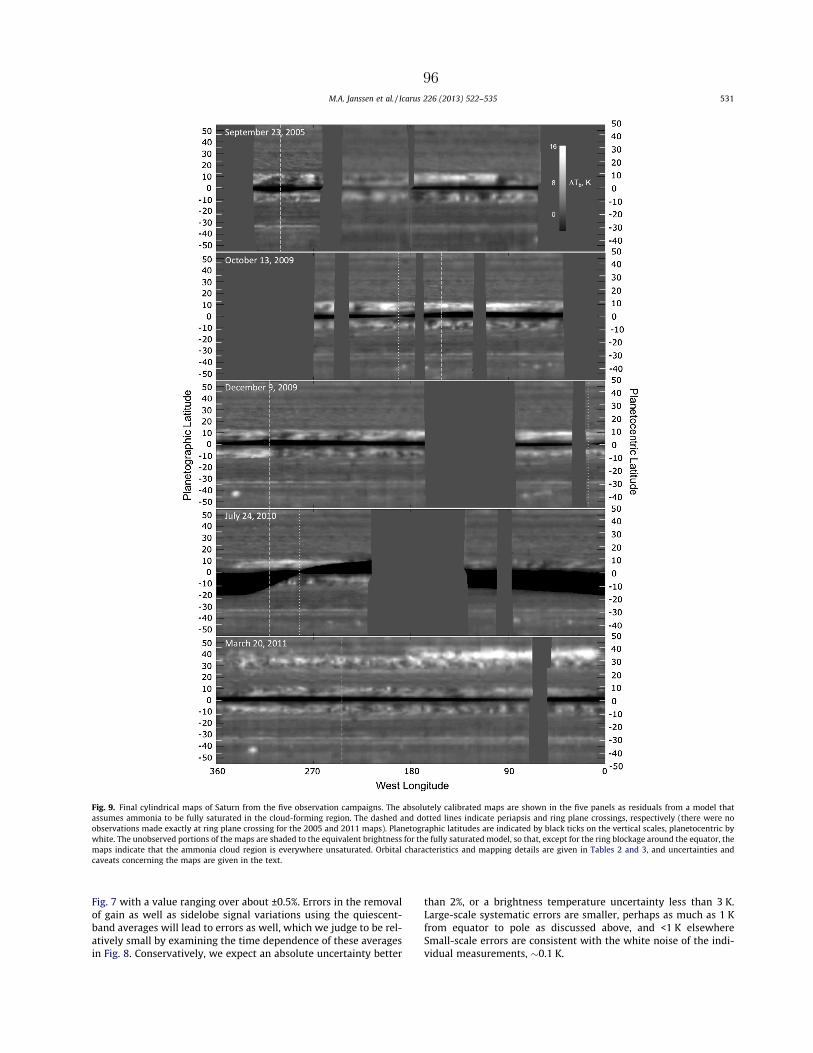
Fig. 7 with a value ranging over about ±0.5%. Errors in the removalof gain as well as sidelobe signal variations using the quiescent-band averages will lead to errors as well, which we judge to be rel-atively small by examining the time dependence of these averagesin Fig. 8. Conservatively, we expect an absolute uncertainty better

than 2%, or a brightness temperature uncertainty less than 3 K.Large-scale systematic errors are smaller, perhaps as much as 1 Kfrom equator to pole as discussed above, and <1 K elsewhereSmall-scale errors are consistent with the white noise of the indi-vidual measurements, 0.1 K.

Fig. 9. Final cylindrical maps of Saturn from the five observation campaigns. The absolutely calibrated maps are shown in the five panels as residuals from a model thatassumes ammonia to be fully saturated in the cloud-forming region. The dashed and dotted lines indicate periapsis and ring plane crossings, respectively (there were noobservations made exactly at ring plane crossing for the 2005 and 2011 maps). Planetographic latitudes are indicated by black ticks on the vertical scales, planetocentric bywhite. The unobserved portions of the maps are shaded to the equivalent brightness for the fully saturated model, so that, except for the ring blockage around the equator, themaps indicate that the ammonia cloud region is everywhere unsaturated. Orbital characteristics and mapping details are given in Tables 2 and 3, and uncertainties andcaveats concerning the maps are given in the text.

M.A. Janssen et al. / Icarus 226 (2013) 522–535 531

96

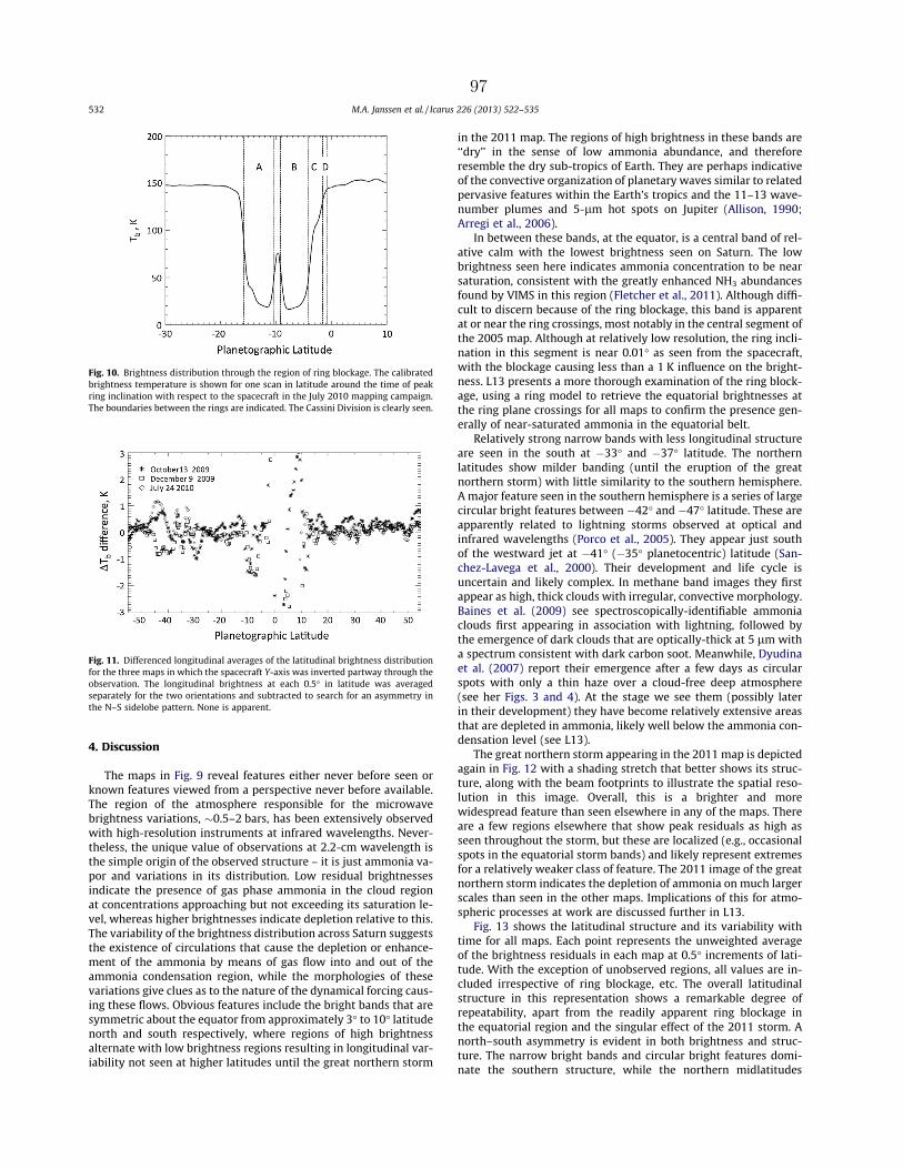
4. Discussion

The maps in Fig. 9 reveal features either never before seen orknown features viewed from a perspective never before available.The region of the atmosphere responsible for the microwavebrightness variations, 0.5–2 bars, has been extensively observedwith high-resolution instruments at infrared wavelengths. Never-theless, the unique value of observations at 2.2-cm wavelength isthe simple origin of the observed structure – it is just ammonia va-por and variations in its distribution. Low residual brightnessesindicate the presence of gas phase ammonia in the cloud regionat concentrations approaching but not exceeding its saturation le-vel, whereas higher brightnesses indicate depletion relative to this.The variability of the brightness distribution across Saturn suggeststhe existence of circulations that cause the depletion or enhance-ment of the ammonia by means of gas flow into and out of theammonia condensation region, while the morphologies of thesevariations give clues as to the nature of the dynamical forcing caus-ing these flows. Obvious features include the bright bands that aresymmetric about the equator from approximately 3 to 10 latitudenorth and south respectively, where regions of high brightnessalternate with low brightness regions resulting in longitudinal var-iability not seen at higher latitudes until the great northern storm

in the 2011 map. The regions of high brightness in these bands are‘‘dry’’ in the sense of low ammonia abundance, and thereforeresemble the dry sub-tropics of Earth. They are perhaps indicativeof the convective organization of planetary waves similar to relatedpervasive features within the Earth’s tropics and the 11–13 wave-number plumes and 5-lm hot spots on Jupiter (Allison, 1990;Arregi et al., 2006).

In between these bands, at the equator, is a central band of rel-ative calm with the lowest brightness seen on Saturn. The lowbrightness seen here indicates ammonia concentration to be nearsaturation, consistent with the greatly enhanced NH3 abundancesfound by VIMS in this region (Fletcher et al., 2011). Although diffi-cult to discern because of the ring blockage, this band is apparentat or near the ring crossings, most notably in the central segment ofthe 2005 map. Although at relatively low resolution, the ring incli-nation in this segment is near 0.01 as seen from the spacecraft,with the blockage causing less than a 1 K influence on the bright-ness. L13 presents a more thorough examination of the ring block-age, using a ring model to retrieve the equatorial brightnesses atthe ring plane crossings for all maps to confirm the presence gen-erally of near-saturated ammonia in the equatorial belt.

Relatively strong narrow bands with less longitudinal structureare seen in the south at 33 and 37 latitude. The northernlatitudes show milder banding (until the eruption of the greatnorthern storm) with little similarity to the southern hemisphere.A major feature seen in the southern hemisphere is a series of largecircular bright features between 42 and 47 latitude. These areapparently related to lightning storms observed at optical andinfrared wavelengths (Porco et al., 2005). They appear just southof the westward jet at 41 (35 planetocentric) latitude (San-chez-Lavega et al., 2000). Their development and life cycle isuncertain and likely complex. In methane band images they firstappear as high, thick clouds with irregular, convective morphology.Baines et al. (2009) see spectroscopically-identifiable ammoniaclouds first appearing in association with lightning, followed bythe emergence of dark clouds that are optically-thick at 5 lm witha spectrum consistent with dark carbon soot. Meanwhile, Dyudinaet al. (2007) report their emergence after a few days as circularspots with only a thin haze over a cloud-free deep atmosphere(see her Figs. 3 and 4). At the stage we see them (possibly laterin their development) they have become relatively extensive areasthat are depleted in ammonia, likely well below the ammonia con-densation level (see L13).

The great northern storm appearing in the 2011 map is depictedagain in Fig. 12 with a shading stretch that better shows its struc-ture, along with the beam footprints to illustrate the spatial reso-lution in this image. Overall, this is a brighter and morewidespread feature than seen elsewhere in any of the maps. Thereare a few regions elsewhere that show peak residuals as high asseen throughout the storm, but these are localized (e.g., occasionalspots in the equatorial storm bands) and likely represent extremesfor a relatively weaker class of feature. The 2011 image of the greatnorthern storm indicates the depletion of ammonia on much largerscales than seen in the other maps. Implications of this for atmo-spheric processes at work are discussed further in L13.

Fig. 13 shows the latitudinal structure and its variability withtime for all maps. Each point represents the unweighted averageof the brightness residuals in each map at 0.5 increments of lati-tude. With the exception of unobserved regions, all values are in-cluded irrespective of ring blockage, etc. The overall latitudinalstructure in this representation shows a remarkable degree ofrepeatability, apart from the readily apparent ring blockage inthe equatorial region and the singular effect of the 2011 storm. Anorth–south asymmetry is evident in both brightness and struc-ture. The narrow bright bands and circular bright features domi-nate the southern structure, while the northern midlatitudes

Fig. 10. Brightness distribution through the region of ring blockage. The calibratedbrightness temperature is shown for one scan in latitude around the time of peakring inclination with respect to the spacecraft in the July 2010 mapping campaign.The boundaries between the rings are indicated. The Cassini Division is clearly seen.

Fig. 11. Differenced longitudinal averages of the latitudinal brightness distributionfor the three maps in which the spacecraft Y-axis was inverted partway through theobservation. The longitudinal brightness at each 0.5 in latitude was averagedseparately for the two orientations and subtracted to search for an asymmetry inthe N–S sidelobe pattern. None is apparent.

532 M.A. Janssen et al. / Icarus 226 (2013) 522–535

97

show repetitive banding at approximately 10 spacing. Residualbrightness temperatures in the region from about 15 to 30are almost as low as those in the central equatorial band inside3. Finally, the north equatorial band from 3 to 10 shows signif-icant variability, while its southern counterpart appears relativelyconstant. We have no simple explanation for the asymmetries wesee. These may have to do with seasonal variations, or may reflectsome degree of chaos in Saturn’s large-scale circulations. For exam-ple, Jupiter has a small obliquity compared to Saturn, but has dem-onstrated considerable and apparently chaotic variability in belt-zone structure over the decades. Seasonal shadowing by Saturn’srings resulting from its large obliquity could lead to seasonal vari-ations between hemispheres if solar forcing were significant indriving circulations. We call attention to the structural asymmetryin the banding apparent in the maps of Fig. 9 from approximately10 to 30 latitude, best seen in the high-resolution segment of the2005 map. The southern hemisphere in this region shows faint butdiscernably regular banding, while the northern counterpart ap-pears mottled. The latter was in the ring shadow in 2005 and theirregular appearance may reflect a lack of solar forcing.

We use a simple variation on our reference model to illustratethe dependence of the brightness residuals on ammonia distribu-tion in this figure. As in the reference model we assume a constantdeep ammonia mixing ratio of 3 solar, however, above its con-densation level we assume a constant relative humidity, the value

of which we allow to vary (this is equivalent to the parameter DFcb

in L13). For example, the light solid line in Fig. 4 shows such a casefor a cloud relative humidity of 50%. The dotted lines in Fig. 13show the brightness then expected for a given cloud relativehumidity, which varies weakly as a function of the viewing geom-etry and is aliased closely with latitude. Our immediate interpreta-tion is that most of the brightness structure seen throughout themaps can be explained by varying ammonia concentrations inthe cloud region alone. The exceptions are the equatorial brightbands bracketing the equator, the circular bright features seen be-tween 42 and 47 latitude, and the northern storm in the 2011map, all of which have regions that cannot be explained unlesssubcloud ammonia is depleted as well. The companion paper L13considers the effect of subcloud mixing ratios using a more realisticmodel involving both cloud-level and subcloud variations inammonia concentration.

5. Conclusions

The advantage of proximity gained from a spacecraft platformhas enabled a significant advance to be made in observing Saturnin the microwave region. Earth-based platforms such as the VLAand more recent millimeter and submillimeter arrays have pro-vided the best imaging results on Saturn prior to this work, buttheir capabilities are limited by the aperture synthesis approachthey require. Although theoretically capable of higher spatial reso-lution and sensitivity, reported VLA images of Saturn in the centi-meter-wavelength region show 0.9 arcsec resolution at best,equivalent to 6 latitude at the equator, with brightness temper-ature sensitivity >1 K. Broad latitudinal banding has been observedunder these conditions, and the use of multiple frequencies has en-abled useful interpretations of the distribution of absorbers (Gross-man et al., 1989; Grossman, 1990; van der Tak et al., 1999).However, longitudinal structure on rotating planets is difficult toobtain by aperture synthesis, and has never been attempted forSaturn. The present maps resolve latitudinal structure as small as1 and longitudinal structure to 2, a significant improvement.Our absolute calibration of 2% represents an improvement by atleast a factor of two as well. The sensitivity for features on smallscales, as good as 0.1%, appears to be over an order of magnitudebetter, while the largest remaining source of error is the possibilityof a systematic error of 1 K that is symmetric about the equator.

As a result we see structure at resolutions approaching thoseachieved by ground-based optical and infrared telescopes, and be-gin to identify features that appear related to those seen bothfrom ground and space at these shorter wavelengths. Our 6-yearbaseline and excellent stability allows us to contribute to the

Fig. 12. The great northern storm of 2010. The section of the March 2011 map containing the storm is shown in the upper panel with a stretch that enhances the highbrightness regions. The lower panel gives the half-power footprints (showing only every fourth footprint in latitude).

Fig. 13. Longitudinal averages of the latitudinal brightness distribution for allmaps. The equatorial region within 5 is generally dominated by ring blockage, as isthe region from 20 to 0 for the July 2010 map – the plunge to negative residualsin these regions is an artifact of this. The dotted lines indicate model brightnessresiduals that would be observed if cloud relative humidity were allowed to varyrelative to the fully saturated model.

M.A. Janssen et al. / Icarus 226 (2013) 522–535 533

98

question of Saturn’s long-term stability. We find that Saturn’sbrightness has been remarkably stable over this period at mostlatitudes, with variations much less than 1%. Exceptions includethe north equatorial bright band, possibly the southern storm al-ley around 45 latitude, and the great storm in the March 2011map. These contrast with time variability seen by the VLA in thelate 1980s and early 1990s, where van der Tak et al. (1999) reportsubstantial latitudinal brightness variations in both hemispheres.We also see a southern hemisphere that is somewhat (1%) cool-er than the north, while van der Tak et al. see a southern hemi-sphere from 1990 to 1995 that was brighter than the northernby 5%, at wavelengths of 2 and 6 cm. Some of the variabilitymay be due to the different wavelengths used and the insensitiv-ity of the 2.2-cm emission to atmospheric temperature and sub-cloud ammonia variations; however, the 2-cm VLA bandingseen earlier by van der Tak et al. is clearly different than the2005–2011 results presented here and implies the existence oflong-term variability in our ‘‘quiescent’’ bands. For example, astorm equivalent to the 2010–2011 storm might have been pres-ent in the southern hemisphere at that time. Unlike the northernstorm, however, it must have persisted for 5 years to explain theobservations, which we consider unlikely. One more global equa-torial map is planned for 2015, which will extend our time baseto 10 years if successful, allowing us to further address the ques-tion of long-term variability. Finally, improvements to the VLAand the coming on-line of new millimeter-wavelength arraysshould enable this question to be pursued for many more years,using the present results as a baseline.

We have limited our interpretation to that allowed by the pres-ent observations themselves, noting that L13 goes more thor-oughly into interpretations involving both the horizontal thevertical ammonia distribution and relates them to dynamical mod-els for the circulations. We also remark that the 2.2-cm radiometricmapping campaign was part of a combined effort with the VisualInfrared Mapping Spectrometer (VIMS) on Cassini that was begunafter the 2005 radiometer mapping effort proved successful. Thisconsisted of VIMS observations of the same regions imaged bythe microwave radiometer both before and after the pass so thatwind-corrected overlays of the infrared maps with the microwavemaps could be examined. Since the VIMS instrument observes thesame pressure range of the atmosphere but is affected by otherconstituents (clouds and haze in particular), questions concerningcirculations and related processes can be examined more fully.Work is currently in progress to compare the VIMS and microwavemapping. Further, the calibrated data and derived maps from thepresent work have been submitted to the Atmospheres Node ofthe Planetary Data System and will be available for comparativestudies in general around the time of the publication of this paper.Lastly, interpretations of the present results are limited becauseonly one frequency was used. Improved VLA capabilities and futuremissions using multiple microwave frequencies can achieve muchmore in understanding the deep circulations and vertical structureof the microwave-active constituents ammonia and water. Forexample, the Juno mission currently on route for arrival at Jupiterin 2016 carries a six-frequency microwave radiometer that will ob-serve Jupiter’s deep atmosphere to pressures greater than 100 barswith such a goal (Janssen et al., in preparation).

Acknowledgments

This research was conducted at the Jet Propulsion Laboratory(JPL), California Institute of Technology, under contract with theNational Aeronautics and Space Administration (NASA). It is partlybased upon work supported by NASA under Grant No. 10-CDAP10-0051 issued through the Cassini Data Analysis and ParticipatingScientist (CDAPS) Program. We acknowledge Sushil Atreya, Lena

Adams, and Virgil Adumantroi for their invaluable contributionsto the Juno Atmospheric Microwave Radiative Transfer (JAMRT)program, P. Steffes for discussions on the microwave absorptionof ammonia in the Saturn atmosphere, Scott Bolton, Steve Levin,and the Juno project for their encouragement of this work, AliceLe Gall for her contributions to the calibration, Bryan Butler for dis-cussion of the capabilities of ground-based interferometers, andGlenn Orton for useful discussions on sources of microwaveabsorption as well as related visual and infrared observations ofgiant planet atmospheres. We also gratefully acknowledge the Cas-sini RADAR team in general for their support, along with those whodesigned, developed and operate the Cassini/Huygens mission,which is a joint endeavor of NASA, the European Space Agency(ESA), and the Italian Space Agency (ASI) and is managed by JPL/Caltech under a contract with NASA.

References

Allison, M., 1990. Planetary waves in Jupiter’s equatorial atmosphere. Icarus 83,282–307.

Arregi, J. et al., 2006. Phase dispersion relation of the 5-micron hot spot wave from along term study of Jupiter in the visible. J. Geophys. Res. 111, E09010. http://dx.doi.org/10.1029/2005JE002653.

Atreya, S.K., 1986. Atmospheres and ionospheres of outer planets and theirsatellites. Springer-Verlag.

Atreya, S.K., 2010. Atmospheric moons Galileo would have loved. In: Galileo’sMedicean Moons – Their Impact on 400 Years of Discovery. CambridgeUniversity Press, pp. 130–140 (Chapter 16).

Baines, K.H. et al., 2009. Storm clouds on Saturn: Lightning-induced chemistry andassociated materials consistent with Cassini/VIMS spectra. Planet. Space Sci. 57,1650–1658.

Berge, G.L., Gulkis, S., 1976. Earth-based radio observations of Jupiter: Millimeter tometer wavelengths. In: Gehrels, T. (Ed.), Jupiter. Univ. of Arizona Press, Tucson,pp. 621–692.

Birnbaum, G., Borysow, A., Orton, G.S., 1996. Collision-induced absorption of H2–H2

and H2–He in the rotational and fundamental band for planetary applications.Icarus 123, 4–22.

Borysow, A., Frommhold, L., 1986. Theoretical collision-induced rototranslationalabsorption spectra for the outer planets: H2–CH4 pairs. Astrophys. J. 304, 849–865.

Briggs, F.H., Sackett, P.D., 1989. Radio observations of Saturn as a probe of itsatmosphere and cloud structure. Icarus 80, 77–103.

Cottini, V. et al., 2012. Spatial and temporal variations in Titan’s surfacetemperature from Cassini CIRS observations. Planet. Space Sci. 60, 62–71.

de Pater, I., 1990. Radio images of the planets. Annu. Rev. Astron. Astrophys. 28,347–399.

de Pater, I., Dickel, J.R., 1982. New information on Saturn and its rings from VLAmultifrequency data. In: Proceedings of Planetary Rings/Anneaux des PlanetesConference, Toulouse, France, August 1982 (abstract).

de Pater, I., Dickel, J.R., 1991. Multifrequency radio observations of Saturn at ringinclination angles between 5 and 26. Icarus 94, 474–492.

de Pater, I., Massie, S.T., 1985. Models of the millimeter–centimeter spectra of thegiant planets. Icarus 62, 143–171.

de Pater, I., Dunn, D., Zahnle, K., Romani, P.N., 2001. Comparison of Galileo probedata with ground-based radio measurements. Icarus 149, 66–78.

Deboer, D.R., Steffes, P.G., 1994. Laboratory measurements of the microwaveproperties of H2S under simulated jovian conditions with an application toNeptune. Icarus 109, 352–366.

Deveraj, K., 2011. The Centimeter- and Millimeter-Wavelength AmmoniaAbsorption Spectra under Jovian Conditions. Ph.D. thesis, Georgia Institute ofTechnology, Atlanta.

Dunn, D.E., Molnar, L.A., Fix, J.D., 2002. More microwave observations of Saturn:Modeling the ring with a Monte Carlo radiative transfer code. Icarus 160, 132–160.

Duong, D., 2011. The Complex Dielectric Properties of Aqueous Ammonia from2 GHz to 8.5 GHz in Support of the NASA Juno Mission. M.S. Thesis, GeorgiaInstitute of Technology, Atlanta, GA.

Dyudina, U.A., Ingersoll, A.P., Ewald, S.P., Porco, C.C., Fischer, G., Kurth, W., Desch, M.,Del Genio, A., Barbara, J., Ferrier, J., 2007. Lightning storms on Saturn observedby Cassini ISS and RPWS during 2004–2006. Icarus 190, 545–555.

Elachi, C. et al., 2004. RADAR: The Cassini Titan radar mapper. Space Sci. Rev. 115,71–110.

Fletcher, L.N., Baines, K.H., Momary, T.W., Showman, A.P., Irwin, P.G.J., Orton, G.S.,Roos-Serote, M., Merlet, C., 2011. Saturn’s tropospheric composition and cloudsfrom Cassini/VIMS 4.6–5.1 lm nightside spectroscopy. Icarus 214, 510–533.

Fulchignoni, M. et al., 2005. Titan’s physical characteristics measured by theHuygens Atmospheric Structure Instrument (HASI). Nature 438, 785–791.

Grossman, A.W., 1990. Microwave Imaging of Saturn’s Deep Atmosphere and Rings.Ph.D. thesis, California Institute of Technology.

Grossman, A.W., Muhleman, D.O., Berge, G.L., 1989. High resolution microwaveobservations of Saturn. Science 245, 1211–1215.

534 M.A. Janssen et al. / Icarus 226 (2013) 522–535

99

Gulkis, S., Poynter, R., 1972. Thermal radio emission from Jupiter and Saturn. Phys.Earth Planet. Interiors 6, 36–43.

Gulkis, S.R., McDonough, T.R., Craft, H., 1969. The microwave spectrum of Saturn.Icarus 10, 421–427.

Hanley, T.R., Steffes, P.G., Karpowicz, B.M., 2009. A new model of the hydrogen andhelium broadened microwave opacity of ammonia based on extensivelaboratory measurements. Icarus 202, 316–335.

Hoffman, J.P., Steffes, P.G., DeBoer, D.R., 2001. Laboratory measurements of themicrowave opacity of phosphine: Opacity formalism and application to theatmospheres of the outer planets. Icarus 152, 172–184.

Janssen, M.A., 1993. An introduction to the passive microwave remote sensing ofatmospheres. In: Janssen, M. (Ed.), Atmospheric Remote Sensing by MicrowaveRadiometry. Wiley & Sons, New York, pp. 1–35 (Chapter 1).

Janssen, M.A., Hofstadter, M.D., Gulkis, S., Ingersoll, A.P., Allison, M., Bolton, S.J.,Kamp, L.W., 2005. Microwave remote sensing of Jupiter’s atmosphere from anorbiting spacecraft. Icarus 173, 447–453.

Janssen, M.A., Lorenz, R.D., West, R., Paganelli, F., Lopes, R.M., Kirk, R.L., Elachi, C.,Wall, S.D., Johnson, W.T.K., Anderson, Y., Boehmer, R.A., Callahan, P., Gim, Y.,Hamilton, G.A., Kelleher, K.D., Roth, L., Stiles, B., Le Gall, A.the Cassini RadarTeam, 2009. Titan’s surface at 2.2-cm wavelength imaged by the Cassini RADARradiometer: Calibration and first results. Icarus 200, 222–239.

Jennings, D.E. et al., 2009. Titan’s surface brightness temperatures. Astrophys. J. 691,L103–L105.

Karpowicz, B.M., Steffes, P.G., 2011a. In search of water vapor on Jupiter: Laboratorymeasurements of the microwave properties of water vapor under simulatedjovian conditions. Icarus 212, 210–213.

Karpowicz, B.M., Steffes, P.G., 2011b. Corrigendum to ‘‘In search of water vapor onJupiter: Laboratory measurements of the microwave properties of water vaporunder simulated jovian conditions’’ [Icarus 212 (2011) 210–213]. Icarus 214,783.

Klein, M.J., Gulkis, S., 1978. Jupiter’s atmosphere: Observations and interpretation ofthe microwave spectrum near 1.25-cm wavelength. Icarus 35, 44–60.

Laraia, A., Ingersol, A.P., Janssen, M.A., Gulkis, S., Oyafuso, F.A., Allison, M.D., 2013.Analysis of Saturn’s thermal emission at 2.2-cm wavelength: Spatialdistribution of ammonia vapor. Icarus, this issue.

Lindal, G.F., Sweetnam, D.N., Eshleman, V.R., 1985. The atmosphere of Saturn: Ananalysis of the Voyager radio occultation measurements. Astron. J. 90, 1136–1146.

Lorenz, R.D., 1998. Preliminary measurements of the cryogenic dielectric propertiesof water-ammonia ices: Implications for radar observations of ice satellites.Icarus 136, 344–348.

Mayer, C.H., McCullough, T.P., Sloanaker, R.M., 1958. Observations of Mars andJupiter at a wavelength of 3.15 cm. Astrophys. J. 127, 11–16.

Mohammed, P., 2004. Laboratory measurements of the W band (3.2 mm) propertiesof phosphine (PH3) and ammonia (NH3) under simulated conditions of the outerplanets. J. Geophys. Res. 109, 1–9.

Orton, G., Gustafsson, M., Burgdorf, M., Meadows, V., 2007. A revised ab initio modelfor collision-induced H2–H2 absorption. Icarus 189, 455–459.

Porco, C.C. et al., 2005. Cassini imaging science: Initial results on Saturn’satmosphere. Science 307, 1243–1247.

Sanchez-Lavega, A., Rojas, J.F., Sada, P.V., 2000. Saturn’s zonal winds at cloud level.Icarus 147, 405–420.

Schloerb, F.P., Muhleman, D.O., Berge, G.L., 1979. Interferometric observations ofSaturn and its rings at a wavelength of 3.71 per cm. Icarus 39, 214–231.

Thornton, D.D., Welch, W.J., 1963. 8.35 mm radio emission from Jupiter. Icarus 2,228–232.

van der Tak, F., de Pater, I., Silva, A., Millan, R., 1999. Time variability in the radiobrightness distribution of Saturn. Icarus 142, 125–147.

West, R. et al., 2009. Cassini RADAR sequence planning and instrumentperformance. IEEE Trans. Geosci. Remote Sensing 47, 1777–1795.

Wrixon, G.T., Welch, W.J., 1970. The millimeter wave spectrum of Saturn. Icarus 13,163–172.

M.A. Janssen et al. / Icarus 226 (2013) 522–535 535

100