Observational data sets for model development

Ž .Coastal Engineering 41 2000 125–153www.elsevier.comrlocatercoastaleng

Observational data sets for model development

Andrew Lane a,), Rolf Riethmuller b, Dagmar Herbers b,¨Peter Rybaczok b, Heinz Gunther b, Helmut Baumert c¨

a Proudman Oceanographic Laboratory, Bidston ObserÕatory, Birkenhead, CH43 7RA, UKb Institute of Hydrophysics, GKSS Research Centre, Max-Planck-Str., D-21502 Geesthacht, Germany

c Hydromod Scientific Consulting, P.O. Box 1229, D-22880 Wedel Schleswig-Holstein, Germany

Abstract

The requirements of ‘comprehensive’ or ‘compatible’ observational data sets for developingand verifying models are examined. ‘Compatibility’ over the range of key parameters involvesaccuracy, spatial and temporal extent, and resolution. The importance of documentation isemphasised on all aspects from experimental strategy to sensor calibration. Likewise, maximisingaccessibility involves listing in international directories, quick-view summary facilities as well asdetailed data listings. Such accessibility generally includes: multi-media dissemination involvingthe Internet; printed papers and reports; CD ROMs.

Experiences from two coastal observational experiments are reviewed: Holderness on the UKeast coast and Sylt-Rømø in the German Bight. These examples provide particular illustrations ofthe generalised principles. They extend to usage of satellite, aircraft, radar, ship, surface and seabed moorings, and piles as platforms. Specific capabilities, limitations and idiosyncrasies of arange of instruments are described. Effective monitoring strategies must aim to exploit theassociated synergies between this full range of platforms and instrumentation. q 2000 ElsevierScience B.V. All rights reserved.

Keywords: Currents; Data calibration; Data dissemination; Data documentation; Data processing; Measure-ment strategy; Suspended sediments; Waves

1. Introduction

Development of the predictive power of mathematical models depends strongly onthe availability of high quality, comprehensive observational data sets for: initialisation,

) Corresponding author. Fax: q44-151-653-6269.Ž .E-mail address: [email protected] A. Lane .

0378-3839r00r$ - see front matter q2000 Elsevier Science B.V. All rights reserved.Ž .PII: S0378-3839 00 00029-6

( )A. Lane et al.rCoastal Engineering 41 2000 125–153126

forcing and verification. Sequential improvements through more sophisticated algo-rithms or data assimilation techniques can only be properly assessed as long as the dataare of comparable accuracy and resolution. While such developments have beenimplemented in the field of weather forecasting, there is a lack of comparable data sets

Ž .in marine sciences, especially in the study of suspended particulate matter SPMdynamics in coastal areas. One of the reasons for this is the requisite sensor maintenanceand checks on calibration necessary to maintain data quality over longer time periods,e.g., for measuring SPM concentrations.

Recognising the above, one objective of Pre-operational Modelling in the Seas ofŽ .Europe PROMISE was to assemble and disseminate comprehensive observational data

sets associated with both earlier and on-going field campaigns with a quality sufficientto test and improve present state-of-the-art models. In this paper we discuss the generalrequirements of comprehensive data sets. These ‘guidelines’ are then illustrated using asexamples, data sets from the Holderness area close to the east coast of England and theSylt-Rømø Bight in the DanishrGerman Wadden Sea.

Subsequent sections describe: general ‘guidelines’ to the planning, execution andŽ .processing of test-bed observational data sets Section 2 ; hence, examples from

Ž . Ž .Holderness Section 3 and Sylt-Rømø Section 4 . Section 2 was largely compiled byR. Riethmuller who, along with co-authors from GKSS is responsible for Section 4. A.¨Lane was responsible for the data processing for the Holderness Experiment, and

Ž .acknowledgement is due to the experimentalists listed in Prandle et al. 1996 .

2. General requirements for comprehensive data sets

A ‘comprehensive’ data set must be complete, consistent, well documented andaccessible. The first two attributes are concerned with the quality of the data set; theremainder deal with long-term usability.

ŽAssessing the quality of the data set is a critical aspect of model validation Lynch et.al., 1995 — it cannot simply be regarded as absolute values. In addition to achieving a

Ž .high level of data correctness such as accuracy and consistency , the data set also has toŽbe appropriate for the intended purpose Rothenberg, 1996; Rothenberg and Kameny,

.1994 . These checks are most important before data sets are disseminated to thecommunity, since subsequent applications cannot be foreseen. Extensive documentationon sampling, processing and objectives in generating the data set are, therefore, requiredto provide ready assessment of its potential usefulness for a specific application.

In the following sections, general requirements for a comprehensive data set will bediscussed in detail.

2.1. Formulation of hypotheses

Hypotheses on the governing processes provide the basis for selecting the parametersof the data set and the sampling strategies and methods to be applied. The key processesconsidered and, hence, the formulation of the respective hypotheses, may depend on thetemporal and spatial scales and the study area considered. In the case of SPM dynamics,

( )A. Lane et al.rCoastal Engineering 41 2000 125–153 127

the following hypotheses were found to be applicable both in the Holderness area andthe Sylt-Rømø Bight:

Hypothesis 1. Wave action and tidal currents are the main erosion and resuspensionprocesses, whereas advective fluxes are predominantly associated with tidal currents.

Hypothesis 2. The loss of bed material is mainly triggered during storm events.

Hypothesis 3. Erosion and resuspension of SPM are influenced significantly by sea bedcharacteristics.

Hypothesis 4. Sedimentation of SPM is strongly influenced by the settling velocities ofthe suspended material.

Hypothesis 5. Microturbulence plays a significant role in the tidal cycle of sedimenterosion or resuspension, advection and settling.

2.2. Data accuracy

Despite the best intentions of those making observations, data quality cannot beconstantly verified throughout field campaigns. This is especially true for long-term datasampling, and for parameters that require much effort in sensor maintenance and

Ž .calibration e.g., measuring SPM concentration . Users need to be made aware of theseproblems when data sets are disseminated — they depend on those who produce thedata sets to perform these checks, and to document the results and any corrective stepstaken.

2.3. Completeness

The ‘completeness’ of a data set encompasses the following aspects:

1. The data set should contain all parameters identified in the hypotheses. The parame-ters listed in Table 1, derived from the above hypotheses, form a complete descrip-tion of the SPM dynamics in coastal regions.

Table 1Parameter list for a comprehensive data set for SPM dynamics in shallow coastal waters

Region Parameter Interior Boundary

Atmospheric boundary layer Air pressure xWind x

Water body Water level x xWaves x xCurrent xSalinity x xWater temperature x x

SPM Concentrations x xSettling velocities x

Bottom Bathymetry xSediment type xErosion shear stresses x


2. Data are collected, both from within the study area and along its boundaries.3. Raw and processed data are stored together with the processing programs and a list of

parameters.Ž4. Relevant documentation is included, enabling users to independently interpret and, if

.necessary, process or reprocess the data.

2.4. Consistency

The data set may be described as ‘consistent’ if it satisfies these conditions:

1. Data from different observations andror model calculations can be intercalibrated.Ž2. Data are provided together with their accuracy e.g., in form of standard deviations,

.confidence intervals, statistical errors, systematic errors, etc. .3. They can be transferred onto common temporal and spatial scales.

2.5. Documentation

Documentation, an integral part of a comprehensive data set, serves as a user guideand should facilitate the following:

1. It enables users to assess the appropriateness of the data set for their requirements.2. It identifies the parameters measured.3. It provides a basis to assess the quality of the data set.4. It explains how the data set is referenced and can be retrieved.

ŽThe first three items are essential for data set quality assurance Rothenberg, 1996;.Rothenberg and Kameny, 1994 . The documentation may also include the following:

specification of hypotheses; sampling strategies; accuracy intended and achieved; meth-ods, scales, quality status of parameters; applied programs; persons and institutionsinvolved, etc. These form part of widely used environmental data standards, e.g., the

Ž . Ž .Global Change Master Directory’s GCMD Data Interchange Format DIF operated byŽ .NASA Irvine and Scialdone, 1992 ; the Federal Geographic Data Committee’s Meta-

Ž .data Standard FGDC, 1998 ; the International Council for the Exploration of the SeaŽ .ICES Format used by the European marine researchers. Such documentation isnecessary for community use of the data set; however, it may in future becomesignificantly different from the standards as these are constantly evolving. The solutionto this potential problem is to ensure that the data set is as self-contained andself-explanatory as possible by storing together the data, documentation and software

Ž .with which the data were created Rothenberg, 1995 . Use of hypertext documents is aneffective means of achieving the above.

2.6. Dissemination

Data sets may be publicised by submitting an entry to catalogue databases, such asŽ . ŽEuropean Directory of Marine Environmental Data EDMED British Oceanographic


. Ž .Data Centre, 1992 , the European Catalogue of Data Sources CDS , or GCMD via itsnational partners. Additionally, the Internet is a relatively inexpensive medium forpublicising and disseminating information, by setting up a website and advertising itthrough search engines. The security, availability and distribution of the data themselvesvia storage media or Internet tools have to be guaranteed by the responsible institutionsover several years.

3. The Holderness data set

3.1. Planning of the Holderness experiment

The Holderness coastline, consisting of rapidly retreating clay cliffs, forms a majorŽ .source of sediment to the North Sea Prandle, 1994a . The aims of the Holderness

Experiment were to monitor the transport of these sediments away from the coast, and tomeasure directly contributions to erosion, suspension and transport.

Major milestones include the following: definition of objectives; consultation ofend-users, collaborators and potential funding organisations; estimation of controllingmechanisms with feedback from a pilot phase. Planning for Holderness incorporated all

Ž .of the latter Prandle, 1994b and Prandle et al., 1996 . Growing widespread interestcontinuously expanded both the goals and the potential scale and scope of the experi-

Ž .ment. As a result the experiment ultimately embraces components concerned with: iŽ .estimating sediment fluxes directly from measurements, ii process studies of specific

Ž . Ž . Žmechanisms e.g., wave-induced bed stress , iii technology development X-band and. Ž .H.F. radar , and iv establishing bench-test data sets for formulating, running and

verifying predictive models.The experiment made use of satellite and aircraft remote sensing, H.F. and X-band

radar, ship surveys, in situ sea bed and sea surface instrumentation. Expenditure wascarefully balanced between capital purchase of instruments required for long-termdeployments, hire over shorter terms, significant costs for data deployment, recovery,losses and subsequent data processing. The guiding principles were concentration on

Ž‘core’ measurements, with duplication in instruments including a range of acoustic,.optical and electromagnetic sensors to cover malfunctioning and questions of calibra-

tion. Likewise, location of fixed rigs in reasonably close proximity allowed questions ofrepresentativeness to be addressed. Conversely, for the more ambitious elements,shorter-term deployments without contingency planning were scheduled.

The major success of the experiment was in synchronising as many as possible of thedisparate elements.

3.2. The obserÕational campaign

Currents, wave parameters, pressure, temperature and conductivity were recordedŽ .together with transmittance and optical and acoustic backscatter, which gave indica-

tions of SPM concentrations. The experiment consisted of three phases; an initialsmall-scale pilot study provided feedback on the range of conditions to be anticipated


Fig. 1. Holderness Coast. Positions of moorings N1–N4, S1–S3.

and an evaluation of the suitability of the rigs and instrumentation. The major experi-ment followed a year later, with a final phase a further year later to complete gaps incoverage.

The pilot study was conducted between November and December 1993. Bottom-Ž .mounted POL-monitoring platforms PMPs were deployed at six mooring sites close to

Ž .the shore Fig. 1 .

3.2.1. Phase one, 1994–1995Ž .In the main Holderness Experiment October 1994–March 1995 , two lines of PMP

stations were located perpendicular to the coast. The northern line consisted of fourŽmoorings three of which were close to the pilot study PMP positions — N1, N2, N3;

. Žone further offshore — N4 and the southern line consisted of three moorings S1, S2.and S3 .

3.2.2. Phase two, 1995–1996Ž .A second Holderness Experiment October 1995–January 1996 concentrated on

Ž .currents and waves at the near-shore sites N1 two sites — N1A and N1B and N2Ž .three sites — N2, N2A and N2B , S1 and S2. These measurements coincided with the


Ždeployment of the OSCR H.F. radar system configured for measuring waves Wyatt and.Ledgard, 1996 .

3.2.3. Concurrent obserÕationsOther observations concurrent with the above experiments included waverider buoys

Ž .at sites N1, N2 and N3 Wolf, 1996a,b ; X-band radar, STABLE, and regular compactŽ . Ž .airborne spectrographic imager CASI flights along the coast. Lane 1997 provides a

description of the instrumentation deployed. The PMPs were used to house an acousticŽ .Doppler current profiler ADCP , a S4 electromagnetic current meter, a high-frequency

Ž .water level pressure recorder and a transmissometer. The rigs closest to the shore wereŽ .equipped with the S4DW, which included an optical backscatter OBS . Acoustic

Ž .backscatter ABS sensors were also used where available.

3.3. Data processing and dissemination

3.3.1. Processing stepsŽ .Separate processing packages one for each type of instrument were developed. The

Ž .programs convert the raw data often given in counts to engineering units. The mooringpositions, calibration coefficients, deployment and data startrend times are stored incontrol files, one for each associated data file. A suite of graphic routines enabled thevisualisation of the data. The quality of the data can be inspected and when necessary,the calibration stage repeated after editing or flagging the raw data.

Many of the routines used in the current processing packages were from KnightŽ .1995 . Software to extract wave parameters from the S4DW and PWR instruments was

Ž .written by Wolf 1996a .

3.3.2. Data disseminationA guiding principle of the experiment was to ensure open access to the data sets

following calibration and quality assurance processing. The data were initially dis-Ž .tributed via the World Wide Web http:rrwww.pol.ac.ukrcoinrHoldernessr and,

subsequently, on a CD ROM from the British Oceanographic Data Centre at theProudman Oceanographic Laboratory.

3.4. Data comparisons and eÕaluations

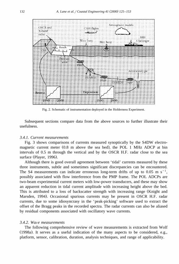
Fig. 2 illustrates the range of instrumentation used, indicating the varying nature ofthe associated coverage. While remote sensing from satellite and aircraft provide

Žoccasional surface snapshots of SPM concentrations subject to complex calibrationrge-.ographical atmospheric correction , most in situ instruments provide continuous long-

term time series but at a single point. By contrast, although radar only measures surfacesignals, it does provide continuous time series. Moreover, for waves, the general validityof linear theory allows such surface signatures to be extrapolated into depth profiles; for

Ž .the X-band radar, this gives an indirect estimation of bathymetry Bell, 1999 . TheADCP is exceptional in providing both vertical current profiles and, subject to interpre-

Ž .tation Holdaway et al., 1999 , SPM profiles.


Fig. 2. Schematic of instrumentation deployed in the Holderness Experiment.

Subsequent sections compare data from the above sources to further illustrate theirusefulness.

3.4.1. Current measurementsFig. 3 shows comparisons of currents measured synoptically by the S4DW electro-

Ž .magnetic current meter 0.8 m above the sea bed , the POL 1 MHz ADCP at binintervals of 0.5 m through the vertical and by the OSCR H.F. radar close to the sea

Ž .surface Player, 1996 .Although there is good overall agreement between ‘tidal’ currents measured by these

three instruments, subtle and sometimes significant discrepancies can be encountered.The S4 measurements can indicate erroneous long-term drifts of up to 0.05 m sy1,possibly associated with flow interference from the PMP frame. The POL ADCPs aretwo-beam experimental current meters with low-power transducers, and these may showan apparent reduction in tidal current amplitude with increasing height above the bed.

ŽThis is attributed to a loss of backscatter strength with increasing range Knight and.Marsden, 1994 . Occasional spurious currents may be present in OSCR H.F. radar

currents, due to some idiosyncrasy in the ‘peak-picking’ software used to extract theoffset of the Bragg peaks in the recorded spectra. The radar currents can also be aliasedby residual components associated with oscillatory wave currents.

3.4.2. WaÕe measurementsThe following comprehensive review of wave measurements is extracted from Wolf

Ž .1998a . It serves as a useful indication of the many aspects to be considered, e.g.,platform, sensor, calibration, duration, analysis techniques, and range of applicability.

()

A.L

aneet

al.rC

oastalEngineering

412000

125–

153133

Ž . Ž .Fig. 3. Comparison of current measurements at N1 minimum water depth of 12 m . North–south component of tidal currents measured by: H.F. radar OSCR at theŽ . Ž .sea surface; S4DW current meter at the sea bed 1 Hz grey, 20 min average black ; POL ADCP odd numbered bins .


Wave data were obtained from the OSCR H.F. radar, a coastal deployment of X-bandradar, nondirectional and directional Waverider buoys, bottom-mounted S4DW currentmeters and pressure sensors, as well as from beach pressure sensors and SAR images.The remote-sensing systems generally provide wave-number spectra over a finite arearather than the frequency spectra obtained from single-point mooring systems.

ŽAnalysis of wave data is by statistical methods because the nature of real sea waves.is an essentially random process . Background on the analysis of pressure data for wavesŽ . Ž . Ž .is given in Bishop and Donelan 1987 , Lee and Wang 1984 . Tucker 1991, 1993

discusses standard analysis of wave data. The details of statistical analysis have beenŽ . Ž .worked out elsewhere, e.g., Long 1980 , Krogstad 1991 . It is also necessary to

attempt to distinguish between various sources of error due to the instrument, calibrationor sampling variability. Details of the processing and calibration are given, for example,

Ž . Ž .by Barstow et al. 1985 and Wolf 1997 . Further discussion of the intercomparison ofŽ .other wave measuring systems is treated elsewhere, e.g., Krogstad et al. 1999 . Here,

we concentrate on the data from the bottom-mounted pressure sensors and S4DWwave-current meters and the surface-following Waverider buoys. The aims are the

Ž .identification of instrumental characteristics strengths and weaknesses and identifica-tion of most useful methods of data intercomparison from a practical point of view. The

Ž .following conclusions were drawn Wolf, 1996b .Ž . Ž .1 The bottom pressure instruments PWR and S4DW provide a robust bottom-

Žmounted system, which should be able to withstand severe weather conditions even a.hurricane as in Taylor and Trageser, 1990 . They are particularly good for long-period

waves, especially swell and for higher sea states. The disadvantage is the depthlimitation due to attenuation of high frequency waves. A bottom-mounted deployment isuseful in that it also provides total water levels. The limit of usefulness is about 20 mdepth. Since high frequency waves are not recorded this type of instrument is poor forfetch-limited growth. The results are good for swell. The Waverider has a resonantresponse at the low frequency end of the spectrum, and the bottom pressure instrumentsmay thus be more accurate for frequencies less than 0.1 Hz. Both PWR and S4DW gavevery similar results up to about 0.25 Hz. The high frequency pressure response of thedifferent transducers may not be identical and problems of drift may occur.

Ž . Ž2 The S4DW instrument measures the p–u–Õ triad pressure and two components.of current . The addition of the current data is very valuable; in particular, it enables the

calculation of wave direction and spread. It also facilitates the improved computation ofwave number and depth-attenuation. However, examination of the mean currents show

Ž y1 .an asymmetry between deployments offsets of a few cm s , suggesting possibleinterference from the supporting frame. A larger frame or a different mounting for theS4DW on the POL PMP is needed.

Ž .3 The advantage of the Waveriders is in their simplicity of deployment, which canbe carried out from a small boat. The instruments are robust and they have beenextensively used for wave measurements, but systematic errors may be being acceptedwithout query. A worrying feature is the low-frequency resonance, which makes theminaccurate for measurement of long period swell. The mooring is the weak point of thesystem, leading to possible capsize in high sea states, underestimates of highest wavesand resonant overestimates of energy at low frequencies. The recommendation for two


elastic strops to be used in the compliant mooring may not be practicable in veryshallow water. In shallow water, the lack of measurement of total water depth andambient current is a limitation, preventing accurate determination of wave number.There is also a possible underestimate of energy at high frequencies, which may againbe due to the movement of the buoy on its mooring. It is known that Waverider timeseries are more symmetrical than the real sea state with less sharp crests since thesystem is not a perfect wave follower. The buoy can also avoid the higher crests by

Ž .horizontal displacements in short-crested seas Barstow et al., 1985 . The measurementof wave direction using directional Waveriders is desirable if possible.

Ž .4 The peak wave direction and period are measured satisfactorily by both S4DWand Waverider instruments.

3.4.2.1. WaÕe climate at Holderness. The wave data from the Holderness ExperimentŽwere collected over two successive winters, 1994r1995 and 1995r1996 Wolf, 1996a,

.1999 . The results served to highlight the fact that two winters are insufficient toestablish the wave climate. There are likely to be longer-term variations in wave heightdue to possible variations in the wave height in the North Atlantic possibly related to theNorth Atlantic Oscillation. The differences between the two winters were quite markedŽ .Wolf, 1998a . The first was more typical with prevailing westerly winds and, therefore,the waves were characterised by swell and fetch-limited wave growth. The second

Ž . Ž .winter more atypical had a preponderance of winds from offshore easterlies withcharacteristic wind-sea spectra. The mean spectra from the two phases of the HoldernessExperiment, divided into onshore and offshore wind cases for stations N1 and N2, are

Ž .shown in Fig. 4. Onshore i.e., from east quadrant winds give higher waves and areseen to be more prevalent in the second winter. Offshore winds give typical bimodalspectra where wind-sea and swell can be separately identified. In the Holderness region

Fig. 4. Mean spectra for the first and second phases of the Holderness Experiment, subdivided into onshoreand offshore winds. — site N1, - - - site N2.


the tidal range is up to 5 m with current speeds up to 0.7 m sy1. Significant waveŽ .heights exceeded 3 m on several occasions. The largest waves observed 5.8 m were on

Ž2nd January 1995 at N3. Wave-current interaction can be significant Wolf, 1998b; Wolf.and Prandle, 1999 .

3.4.3. SPM measurementsFig. 5 shows a comparison of SPM time series measured by OBS, transmissometers

and ABS. Each of these instruments has their own calibration peculiarities. Additionally,all of these calibrations vary as the ‘mean’ particle size changes. Since the optical

Ž . Ž .devices rely on occlusion of light transmissometer or reflection OBS , the signal isdependent on the surface area of the particle. The recorded signal, therefore, needs to bemultiplied by a representative particle ‘radius’ to indicate concentration, i.e., theapparent concentrations are more sensitive to finer scale particles. The plate-likecharacter of some fines adds additional complication. Conversely, ABS in the range of

.frequencies used in ABS instruments increases with particle volume and, hence, thisinstrument is more sensitive to coarse particles. Thus, the close agreement indicated inFig. 5 may obscure the sensitivity of the calibrations to variations in particle sizespectra, which occur between sea bed and sea surface, over a tidal period, over thespring-neap tidal cycle, seasonally and during storm and wave ‘events’. The opticalinstruments also experience fouling and all of the instruments can be swamped abovecertain concentrations.

Ž .Fig. 5. Comparison of suspended particulate material SPM concentrations. Concentrations measured byoptical backscatter transmissometer and acoustic backscatter instruments at site S2.


Ž .Fig. 6. Surface distributions of SPM, transmittance uncalibrated units measured from on-board pumpedsampler, 15–16th October 1994.

The SPM distribution in Fig. 6 is based on pumped sample transmissometer measure-Ž .ments on board RRS Challenger Prandle, 1994b . Fortuitously, the associated 3 days of

cruise time coincided with tranquil weather and, hence, the pattern is sensibly synopticŽ .with tidal modulation . The CASI images in Fig. 7 provide similar distributions undercloud free conditions. The associated flight times are less than 1 h and, hence, theseresults are more effectively synoptic. However, the calibration of these images is morecomplex and their availability in cloud free conditions can provide a distorted represen-tation of average conditions.

3.5. Summary

For preoperational model simulations, observational data are required for setup,Ž .initialisation, boundary conditions, forcing, assimilation where employed and verifica-

tion. The provision of accurate fine-scale bathymetry is widely recognised as a majordeficiency in the setup stage. In simulations where the bathymetry evolves dynamically,there is a need for techniques, such as shown in Fig. 8, to monitor this. Initialisation ofSPM simulations involves specification of sea bed deposits ‘available’ for erosion. Thisis a fundamental difficulty sometimes circumvented by a spin-up simulation based onoriginal sources to redistribute these accordingly. Boundary conditions involve specifica-tion of inputs or outputs along the coast, within estuaries and at seaward boundaries ofthe model. Figs. 6 and 7 can be used to provide indications of the more sensitivesections. Forcing by tides, surges or waves along the open boundaries are generally


ŽFig. 7. CASI image of the Holderness coast, 21st September 1995 09:50 LWq30 mins. Raw image courtesy.of the Environment Agency. Image processed by Susan Shimwell at ARGOSS. .

provided by larger-scale ‘preoperational’ modelling simulations — but prescription ofoceanic inputs can be inadequate. Verification data should include the full range of

Fig. 8. X-band radar image of near-shore waves. Contours of derived bathymetry are superimposed.

()

A.L

aneet

al.rC

oastalEngineering

412000

125–

153139

Ž . Ž .Fig. 9. SPM concentrations during 23rd January–6th February 1995 at sites a N1, N2, N3 and b S1, S2, S3.


conditions at sufficient strategicrrepresentative locations. Fig. 9 illustrates examples ofa range of conditions at three representative cross-shore sites. Distinction can be seenbetween intervals of well-ordered tidally dominated regimes and wave-dominatedevents. The importance of tidal advection in regions of strong concentration gradients atsites N1 and N2 differ from the more dispersive regime at station N3. Interpretation of

Ž .these observations by reference to single-point modelling Baumert et al., 2000indicates how the influence of the limited availability of sediments can be deduced.

The various stages are described: planning, implementation, data processing andanalyses of a major observational experiment to provide bench-mark data sets for modelformulation and development. With a focus on simulation of coastal sediment move-ment, the choice and adequacy of a range of instrumentation for measuring currents,waves and SPM distributions have been described. The characteristics of remotesensing, radar, in situ and shipborne instrumentation have been illustrated together withtheir synergistic aspects. The Holderness data set is shown to be well suited fordevelopment of the latest coupled tide-surge-wave models. However, it should be notedthat bathymetric evolution represents the time integration of the spatial divergence ofsediment fluxes. Thus, although present models are often sufficiently accurate toreproduce observed sediment concentrations, this may not be adequate for predictingbathymetric evolution. Clearly, nonlinearities resulting from coupling of wave and tidalmotions and from large amplitude perturbations of each will influence net residualfluxes of sediment. Thus, while this data set is adequate for testing short-term forecasts,further observational data sets will be necessary, including detailed synoptic measure-ments of changes in bathymetry with LIDAR in intertidal regions or from X-band and

Ž .SAR Bell, 1999 , further offshore will be necessary. Likewise, more detailed airborneimagery coincident with in situ calibration data should add further to the value of futureexperiments.

4. The Sylt-Rømø Bight data set

4.1. Description of the Sylt-Rømø

The Sylt-Rømø Bight is a semi-enclosed lagoon located in the North Frisian WaddenŽ .Sea on the Danish–German border see Fig. 10 . A complete description of ecosystem,

Ž .hydrodynamic and sediment properties in the Bight is given by Gatje and Reise 1998¨Ž .and Austen 1996 .

2 ŽThe tidal basin has an area of 400 km of which 67% is subtidal 10% above, 57%.below y5 m in the deep channels and 33% is intertidal. The maximum depth is 40.5 m

at the inlet. This region consists of predominantly sandy flats with mud flats and saltmarsh, each covering -10 km2. The tides are semidiurnal and the mean range is 2 m.Water levels of y3.5 m and q4.0 m have been recorded during prolonged periods ofwind forcing. The low water volume is about 570 m3 and the intertidal volume is of thesame order of magnitude. Maximum depth-averaged currents in the tidal channels are ofthe order of 0.6 m sy1. Salinity remains close to 30–32 psu in most parts sinceatmospheric input and fresh water discharge from rivers are less than one thousandth of


Fig. 10. Landsat TM image of the Sylt-Rømø Bight. Superimposed are locations of instruments and shipsurvey tracks.

the water exchange with the North Sea. Only in the vicinity of the mouths of the Breda˚ ˚A and Vida A does the fresh water input become detectable. The suspended sedimentconcentrations range from a few mg ly1 at the Lister Tief to more than 100 mg ly1

towards the coast at high-water and close to the river mouth where the characteristicestuarine turbidity zones exist.

The Bight is drained through three main tidal channels: the Rømø Dyb in the north˚along the Rømø coast from the mouth of the Breda A; the Højer Dyb in the middle


˚starting at the mouth of the Vida A; and the Lister Ley running north–south along theSylt coast. Two causeways in the north and south connect the islands of Sylt and Rømøwith the mainland. The Bight, therefore, exchanges water with the adjacent North Seaexclusively through one narrow tidal gully, the Lister Tief.

4.2. Experimental objectiÕes — site selection

Previous investigations have shown that the Bight has sustained a significant and stillŽunexplained loss of bed material in the regions close to the low water level Higelke,

. Ž .1998 . Additionally, for fine-grain material diameter-63 mm , the net input rate,averaged over the past thirty years, was found to be ten times smaller than in other

Ž .Wadden Sea back barrier areas Bayerl et al., 1998 . One explanation for the materialloss may be the observed increased frequency of heavy storm floods combined withprogressive coastal protection measures in the last century: more material is stirred intothe water column more often and the usual sediment settling in parallel flat retentionareas ceased.

The Bight is also interesting from a modelling perspective: the area has only oneboundary with the adjacent North Sea. Pilot studies have shown that the currents insidethe Bight are nearly all controlled by the North Sea boundary, which in turn is a functionof tidal phase and wind direction and speed. The water depth in the Bight is typically inthe range 0–20 m, with variations due to subsidence in dry areas. Therefore, theinteraction of currents and waves in very shallow, tidally dominated areas can be studiedwith coupled models. Bed erosion, resuspension of SPM and advective transports arealso expected to depend on: tidal currents in the deeper parts of the gullies, wave actionin the shallow areas. Both mechanisms will act in intermediate regions, the extent andlocation of which migrate with tidal phase and wind conditions.

4.3. Sampling strategies

Based on the hypotheses formulated in Sections 2.1 and 4.2, the quantities required toŽ .study suspended sediment dynamics see Table 1 were recorded both in moderate and

in stormy weather conditions over periods of several months. Two sampling strategiesŽ . Žwere combined: i time series recorded at fixed positions from stable platforms piles,

. Ž .moored ADCPs, wave rider buoy , ii ship cruises between these positions to studyrepresentativeness of the fixed positions and for spatial interpolation and extrapolationof the time series.

Ž .The locations of instruments and cruises are shown in the map Fig. 10 . The fixedinstruments recorded data from April–October 1996 and April–May 1997. Cruises wereconducted in 1996 only: the first from 22nd April–2nd May, the second from the 10th to30th of September. Due to instrument failure and loss, not all of the equipment delivered

Ždata during these periods. Four periods with significant wind events maximum windy1 .speed greater than 15 m s were selected from the PROMISE data set. These were

quality controlled, documented and disseminated. Table 2 gives an outline of therecording periods, instruments and cruises.


Table 2Timetable of deployments and cruises in the Sylt-Rømø Bight

Period Piles ADCP Wave- Cruise 1 Cruise 2rrider PROMIXP1, P2, P3, P4, 1, 2, 3, 4,

Lister Højer Rømø Hunnig- Lister Højer Rømø Lister BightLey Dyb Dyb ensande Ley Dyb Dyb Tief Centre¨

1–15th x x x x x x AprilrJune 1996 May10–30th x x x x x x x x xSeptember 199610–31th x x x xOctober 19961–27th x x x xApril 1997

4.3.1. Time series

4.3.1.1. Piles. At four locations within the Bight, piles were driven into the bed asŽ .carriers for instruments. Three piles P1–P3 were positioned at the side of each of the

main tidal channels. The lateral position was the 2-m-mean low-water line, the optimumlocation considering the maximum pile length for stability and the need to have constantcoverage of instruments when mounted at 1 m above the bed. The longitudinal positionwas chosen to be close to where cross-sectional measurements had been carried out in

Ž . Ž .previous years in the SWAP project Fanger et al., 1998 . The fourth pile P4 waspositioned in a shallow water area at Hunnigensande.¨

ŽEquipment on the piles measured the complete set of parameters except wave.direction and settling velocities and data were regularly transferred via real-time

telemetry to a remote land station. SPM concentrations were determined by opticaltransmission; wave spectra recorded by means of a floater with magnetic readoutmoving freely along a vertical rod. The wave recorders measured water levels at 2 Hz

Ževery 5 min when triggered by a threshold change of 10 cm in water level between.subsequent records . Other data were averaged over 10 min.

4.3.1.2. Moored ADCP systems. Broadband ADCPs were moored at the bed in thechannel close to the main current axis, near to positions P1–P3. The vertical position ofthe transducer heads was some 1 m above the bed to avoid unwated effects of ripples.This was sufficient for most of the time except after strong winds, which caused thedevelopment, and movement of larger bedforms.

The ADCPs recorded time series of vertical profiles of current velocities andbackscatter intensities with a vertical resolution of 0.25 m averaged over 10 min. Thedata were stored on magnetic tapes that were regularly exchanged by divers duringmaintenance work.

4.3.1.3. Directional waÕe rider buoy. In the central part of the Bight, a directional waverider buoy registered both the contributions of the North Sea swell entering through the


Lister Tief and the wind seas generated inside the Bight itself. Current and windconditions, and ship traffic, meant that the position of the buoy had to be altered slightlyduring the data acquisition phases. The wave rider buoy yielded wave heights anddirections for frequencies 0–0.6 Hz. Data were regularly transferred in real-time to aremote land station.

4.3.2. Ship cruisesShip cruises took place during AprilrMay and AugustrSeptember 1996, each lasting

two weeks. The ship tracked back and forth along the main tidal channels over a lengthŽ .of about 15 km see Fig. 10 , the most upstream position was defined by a safety margin

water depth of 3 m. Vertical profiles were taken at 1-km intervals at predefinedpositions. The drift in the ship’s position during data recording was typically about 20m. One of the three tidal channels was covered per day, with sampling over a full tidalcycle, during which up to six longitudinal sections could be covered.

The current velocity profiles were measured by a narrow-band ADCP, profiles ofother hydrographic and SPM parameters were by a vertical profiler recording at 8 Hzwith a fall velocity of 0.25 m sy1. Altogether, some 700 vertical profiles were acquired.

4.3.3. Micro turbulence — PROMIXŽA joint PROMISErMICSOS measurement campaign named PROMIX and funded.by the German project on mixing processes in estuaries was undertaken on 26–27th

September 1996 close to the Højer Dyb station P2rA2. The turbulent microstructureŽwas measured every 15 min by a free-falling profiler from which the total turbulent

.kinetic energy and its dissipation rate can be derived; see Prandke and Stips, 1996Žtogether with SPM concentration for process studies to determine the impact of waves,

.currents and turbulence on SPM dynamics . Vertical profiles of TKE were also derivedŽ .from shipborne narrow-band ADCP data recorded at 1 Hz . A broadband ADCP

moored nearby provided data on local hydrodynamics.

4.3.4. Data processing and quality assuranceData processing was organised into the following steps:

1. The raw data was calibrated to physical values for derived parameters, such assalinity from temperature and conductivity.

2. Spectral moments were calculated from the wave recorder data; SPM concentrationswere obtained from ADCP backscatter and optical transmission sensors in conjunc-tion with filtered water samples.

Ž .3. The data sets were merged together: in time 10 min for the piles and mooredŽ .ADCPs, and in depth 0.25 m for the vertical profiles.

Quality assurance steps were taken at different stages of data generation:

1. Regular recalibrations were made during sampling and sensor maintenance forsensitive devices, such as optical transmissometers or oxygen cells.


Ž .Fig. 11. Left: Observed and modelled tidal dependence of currents at pile P1 Lister Ley ; Right: observedwater depth at P1.

2. The accepted extreme values were derived from existing knowledge about the studyarea before and during data processing through minimumrmaximum criteria.

Fig. 12. Eddy at flood tide in the Sylt-Rømø Bight.


3. Data were inspected visually after processing, e.g., qualitative consistency with tidalphase or weather situation.

Ž .4. Data were compared with model results if available after processing.

Some detailed examples of quality assurance are given below.

( )4.3.4.1. Current Õelocities measured at P1 Lister Ley . The currents were expected tobe mainly alternating with the ebb and flood tide and nearly aligned with the mainchannel axis. This behaviour was observed only for ebb tide; during flood, however,measured current directions rotated away from the channel, indicating that the water was

Ž .flowing from south east over the tidal flats Fig. 11 . Since no instrument failure wasdetected, the data were compared to numerical model simulations for comparable wind

Žsituations using a depth-averaged version of the TRIM model Cassuli and Cattani,. Ž .1994 on a 100-m grid Behrens et al., 1997 . The model results for this location showed

the same structure except for a small offset in current direction. This unexpectedŽ .behaviour is explained by the overall current pattern in this region Fig. 12 . During the

flood, a clockwise eddy develops in the lee spur of the northern Sylt and the currents inthe flats around P1 are refracted away from the gully direction. The differences betweenmodel and data may be explained by the spatial model resolution.

( )4.3.4.2. WaÕe measurements at P3 Rømø Dyb . The time series of significant waveŽheight computed from the estimated power spectra showed considerable scatter Fig.

.13 . Close inspection of the 2-Hz time series exhibited a number of outliers, which werereplaced at first by interpolating between the two neighbouring values. Next, the timeseries with more than one outlier in a row were completely rejected from further

Ž .Fig. 13. Wave height computed from time series for the periods 7–14th April 1997 at pile P3 Rømø Dyb .Upper panel from original time series, lower panel from corrected time series.


processing. The time series with significant wave heights from the corrected spectra thenshowed smoother behaviour, comparable to that from the wave rider buoy data. This

Ž .correction procedure was applied to the wave measurements at all stations P1–P3 .

4.3.4.3. SPM concentration from optical transmission. SPM concentrations were derivedfrom optical transmission. The relationship between the optical attenuation coefficientsand the SPM concentration was derived from repeated calibration with water samplestaken in parallel, which had been pressure filtered. The transmissometers both on thepiles and on the vertical profiler were identical and had been used previously in theSWAP project. During SWAP, extensive calibration had been performed in all tidalgullies, over a number of tidal cycles. The full data set could be described well by a

Ž .single calibration function, which accounted for over 80% of the variance Fig. 14 .During the PROMISE ship cruises, fewer samples were taken, but much higher SPMconcentrations were experienced. The calibration function obtained is fully compatiblewith the SWAP result, which does not appear to be time-dependent and is valid over theentire survey area.

The main obstacle to deriving reliable SPM concentrations from optical transmissionat the pile sites is the unpredictable fouling of the optical devices after maintenance. Itseffect is clearly visible, but to find an almost unbiased correction for this is very difficultand has as yet not been done. Quality assurance strategy in this case is to provide adescription of the status quo, namely: to present the optical attenuation coefficients andcalibration curves as separate entities and to warn users not to apply this function to theoptical data without scrutiny. In future, all corrections applied will define new levels ofprocessed data that have to be described carefully in the documentation of the data set.

4.3.5. Boundary dataThe data set contains boundary data for the:

Ø bathymetry;Ø tidal elevation at the North Sea boundary across the Lister Tief;Ø SPM concentrations at a position close to the North Sea boundary;

Ž . ŽØ local wind fields, depth-averaged currents Behrens et al., 1997 and waves Schneg-.genburger, 1998; Schneggenburger et al., 1998 within the Bight from numerical

model calculations.

Technical details on the generation of the boundary data are given in the referencesand the documentation files of the data set.

4.3.6. DocumentationData set documentation is provided at four levels: data set, sampling device, probes

and parameters, data values. The documentation structure listed in Table 3 correspondsŽ .to the format of the CERA-2 Metadata Model Lautenschlager et al., 1998 , the standard

structure for climate research in Germany. This type of documentation satisfies the

()

A.L

aneet

al.rC

oastalEngineering

412000

125–

153148

Fig. 14. Calibration curves for optical attenuation in PROMISE and SWAP.


Table 3List of documentation parameters for the PROMISErSylt-Rømø data set

Data set Sampling device Probes and Data valuesparameters

Entry project title, objectives, type meaning horizontalmain hypotheses, sampling positionintended scales and coordinates of physical units verticalaccuracy, sampling position sampling positionstrategies, keywords, list of probes abbreviations sampling timelinks to related data sets list of measured and probe resolution merge interval

Ž .derived parameters space, time

Publications comprehensive data run-charts probe accuracy No. of mergedreport, scientific datapublication related data processing calibration standardto the data set levels procedures deviation of

merged datasoftware source calibrationcode functions

Contact addresses of institutions data file quality statusand persons involved description during sampling

Spatial coordinate systems used version ofinformation processing level

Coverage spatial and temporal applied qualityrange covered by the assurancedata, maps, time schedule methodof devices and gadgets quality status ofprobes processing level

Status information on data set achievedversion and data accuracy inprocessing applied processing level

Dissemination storage devices, formats,access authority

Ž .‘Skinny DIF Standard’ NASA, 1998 of the GCMD, and is adapted to match the FGDCŽ .metadata standard FGDC, 1998 .

4.3.7. DisseminationTo make the data retrievable by the community, it has been reported to the EDMED

catalogue. Additionally, it is included in the Land Ocean Thematic data Search EngineŽ .LOTSE developed at the GKSS Research Centre to document interdisciplinary

Ž .research and monitoring projects on German coasts Gehlsen et al., 1999 . The docu-mentation in the LOTSE-project-homepages is compatible with the ‘Skinny-DIF Stan-dard’. Links to data sources are included, which can be of any format, ranging fromhighly advanced systems, such as relational databases to simple ASCII files. The


LOTSE-project-homepages are regularly scanned by most of the Web search enginesmaking them searchable worldwide.

The data set is password-protected but will be made available on request for scientificand administrative purposes. A pilot system guides users through the documentation aswell as the data files. The data set, including the pilot system, is also stored on CDROM, the status of the information has been updated to the end of the PROMISEproject. Subsequent updated versions will be available via the Internet.

5. Summary and conclusions

The requirement for comprehensive observational data sets against which to developnumerical models is universally recognised. However, elucidation of what constitutes‘comprehensive’ is rarely rigorously examined. The PROMISE project provided experi-ence in exchanging such data sets between partners for use with a range of models.These exchanges emphasised the necessity for rationalised protocols and also theopportunity to address this question from a generalised perspective. The account of these

Žexperiences reported here provide useful complementarity for subsequent papers in this.volume on related modelling studies and, hopefully, useful guidelines for future

planning of such observational experiments.The broader interrelationships between observational data sets and modelling are

summarised in Fig. 1 of the Introduction to this volume. The data sets must be adequatein quality, i.e., be sufficiently complete and be consistent with the model, and be usable,i.e., well documented and accessible. Completeness requires overlapping in range ofparameters, duration and spatial extent; consistency infers compatibility in accuracy, and

Žin both spatial and temporal resolution. Documentation must indicate suitability espe-.cially for ‘third-party’ future users , usability, and must include details of the overall

strategy, platforms and sensors as well as actual data and their quality status. Accessmay involve several media, typically an international data inventory for initial locationŽ .permitting Internet search system , an Internet homepage for graphical summaries and aCD ROM for ‘permanent’ raw-data exchange. As much effort needs to be invested todocument the data sets and make them readily accessible as in the data processing andquality assurance itself.

Specific experience from two coastal observational experiments are then reviewed,Holderness on the UK east coast and Sylt-Rømø in the German Bight. The value of an

Ž .initial pilot phase is indicated and the importance of duplication sensors and systems in‘core’ observations together with the choice between usage of satellite, aircraft, radar,ships, buoys, sea bed moorings and piles as platforms is illustrated. Recognition of thesynergies between such observations and the importance of synchronisation is empha-sised. Resources are always limited and selection of strategicrrepresentative sectionsand locations for monitoring is important. Observational system sensitivity experimentsmay be valuable at this stage.

Examples of the peculiar characteristics of both sensors and platforms are reported.Attention to quality assurance is shown to be necessary at four stages, during samplingŽ . Ž .biofouling, etc. , during processing basic checks , via post-processing ‘visual’ inspec-


tion and during observation-model intercomparisons, which must allow for calibrationerrors, etc.

Ž .Finally, referring again to Fig. 1 in the Introduction Prandle, 2000 , the usefulness ofbench-test data sets will depend critically on: the accuracy and resolution of setup dataŽ .bathmetry, surficial sediments, etc. ; boundary and surface exchanges from associated

Ž .marine, atmospheric and terrestrial modelling systems; and specification of empiricalor nonmeasured parameters where necessary.

Acknowledgements

Ž .The Holderness Experiment originated as part of the UK Natural EnvironmentŽ .Research Counsil’s NERC LOIS project. The comprehensive data set subsequently

Ž .contributed and was supported by a number of related studies, namely: i CAMELOTŽ . Ž .contract FD311 of MAFF’s Flood Defence Commission with NERC ; ii Surface

Ž .Current and Wave Variability Experiment — SCAWVEX Wyatt et al., 1995 . MASTŽ . Ž . Ž .II coordinator: L. Wyatt, University of Sheffield. MAS2-CT940103 ; iii Pre-oper-

Žational Modelling in the Seas of Europe — PROMISE. MAST III coordinator: D.. Ž .Prandle, Proudman Oceanographic Laboratory. MAS3-CT950025 . The Sylt-Rømø

data sampling was funded by the Bundesministerium fur Bildung und Wissenschaft,¨Ž .Forschung und Technologie BMBF . GKSS would like to thank: the Wattenmeerstation

of the Biologische Anstalt Helgoland for hosting staff and supporting the field andmaintenance work; Dr. M. Pejrup from the University of Copenhagen for technical andadministrative support; the German and Danish Water Authorities for permission tomoor instruments in the respective waters of the Sylt-Rømø Bight; and the Amt fur¨Wehrgeophysik for providing North Sea wave data. The setup and maintenance of themany instruments was made possible by the encouragement of GKSS staff: H. Belau, H.Bornhoft, G. Bottcher, H. Garbe, P. Perthum, M. Pose, R. Matheisel, B. Puch, R.¨ ¨Reshoft, S. Schmidt and G. Schymura. A. Behrens and G. Gayer and C. Schneggen-¨burger from the Institute of Hydrophysics at the GKSS Research Centre delivered theSylt-Rømø Bight model results and water level data. Dr. W. Puls provided the North SeaSPM boundary values.

References

Austen, G., 1996. Qualitative und quantitative Untersuchungen an Schwebstoffen im Sylt-Rømø WattenmeerŽ .Thesis, in German , Berichte aus dem Forschungs- und Technologiezentrum Westkuste der Universitat¨ ¨Kiel Nr. 11, Kiel, ISSN 0940-9475.

Barstow, S.F., Krogstad, H.E., Torsethaugen, K., Audunson, T., 1985. Procedures and problems associatedwith the calibration of wave sensors. Advances in Underwater Technology and Offshore Engineering.Evaluation, Comparison and Calibration of Oceanographic Instruments vol. 4, Graham and Trotman,London, pp. 55–82.

Baumert, H., Chapalain, G., Smaoui, H., McManus, J.P., Yagi, H., Regener, M., Sundermann, J., Szilagy, B.,¨2000. Modelling and numerical simulation of turbulence, waves and suspended sediment for preoperationaluse in coastal seas. Coastal Eng., This volume.

ŽBayerl, K.A., Austen, I., Koster, R., Pejrup, M., Witte, G., 1998. Sediment dynamics in the list tidal basin in¨. Ž .German . In: Gatje, Ch., Reise, K. Eds. , The Wadden Sea Ecosystem: Exchange, Transport and¨

Transformation Processes. Springer, Berlin, pp. 127–160.


Behrens, A., Gayer, Gunther, H., Rosenthal, W., 1997. Atlas der Stomungen und Wasserstande in der¨ ¨ ¨Ž . Ž .Sylt-Rømø-Bucht in German . Report of the GKSS Research Centre 97rEr21 ISSN 0344-9629 ,

CD-ROM, 20 pp.Bell, P.S., 1999. Shallow water bathymetry derived from an analysis of X-band marine radar image of waves.

Coastal Eng. 37, 513–527.Ž .Bishop, C.T., Donelan, M.A., 1987. Measuring waves with pressure transducers. Coastal Eng. 11 4 ,

309–328.Ž .British Oceanographic Data Centre BODC , 1992, European Directory of Marine Environmental Data

Ž .EDMED : directory of marine environmental data sets in BODC. British Oceanographic Data Centre,Birkenhead, UKrCommission of European Communities. 44 pp.

Cassuli, V., Cattani, E., 1994. Stability, accuracy and efficiency of a semi-implicit method for three-dimen-sional shallow water flow. Comput. Math. Appl. 4, 99–112.

Fanger, H.-U., Backhaus, J., Hartke, D., Hubner, U., Kappenberg, J., Muller, A., 1998. Hydrodynamics in the¨ ¨Ž .List tidal basin: measurements and modelling in German . The Wadden Sea Ecosystem: Exchange,

Transport and Transformation Processes. Springer, Berlin, pp. 161–184.Ž .FGDC, 1998. Content Standard for Digital Geospatial Metadata CSDGM , Version 2, Federal Geographic

Data Committee, Reston, VA.Ž .Gatje, Ch., Reise, K. Eds. , The Wadden Sea Ecosystem: Exchange, Transport and Transformation Processes.¨

Springer, Berlin.Gehlsen, B., Kriebisch, R., Krasemann, H., Lamersdorf, W., Page, P., Wolff, N., 1999. LOTSE — realisierter

Ž . Ž .Web-Zugriff auf heterogene Datenbestande in German . In: Kramer, R., Hosenfeld, F. Eds. , Heterogene,¨Aktive Umweltdatenbanken. Metropolis, Marburg.

Ž . Ž .Higelke, B., 1998. Morphodynamics of the List tidal basin in German . In: Gatje, Ch., Reise, K. Eds. , The¨Wadden Sea Ecosystem: Exchange, Transport and Transformation Processes. Springer, Berlin, pp.103–126.

Holdaway, G.P., Thorne, P.D., Flat, D., Jones, S.E., Prandle, D., 1999. Comparison between ADCP andtransmissometer measurements of suspended sediment concentration. Cont. Shelf Res. 19, 421–441.

Irvine, D., Scialdone, J., 1992. The global change master directory. Proceedings of the Marine TechnologyŽ . ŽConference. Marine Technology Society, Washington, DC USA , pp. 666–670, MTS ’92: Global Ocean

. Ž .Partnership, Proceedings URL: http:rrgcmd.gsfc.nasa.gov:80r .Knight P.J., 1995. Time series data processing manual. Version 2.0. Proudman Oceanographic Laboratory

Internal Document No. 77, 55 pp. Unpublished manuscript.Knight, P.J., Marsden, R.C., 1994. Current profile, pressure and temperature records from the North Channel

of the Irish Sea from equipment deployed on RRS Challenger cruises C106 and C107. ProudmanOceanographic Laboratory Report No. 35, 141 pp.

Krogstad, H.E., 1991. Reliability and resolution of directional wave spectra from heave, pitch and roll dataŽ .buoys. In: Beal, R.C. Ed. , Directional Wave Spectra. Johns Hopkins Univ. Press, Baltimore.

Krogstad, H.E., Wolf, J., Thompson, S.P., Wyatt, L.R., 1999. Methods for the intercomparison of waveŽ .measurements. Coastal Eng. 37 3–4 , 235–257.

Lane, A., 1997. Currents and SPM measurements. Holderness, East Coast, England. November–December1993, October 1994–February 1995 and October 1995–January 1996. Proudman Oceanographic Labora-tory Report No. 45, 50 pp.

Lautenschlager, M., Toussaint, F., Thiemann, H., Reinke, M., 1998. The Cera-2 Data Model, DeutschesŽ .Klimarechenzentrum, Technical Report No. 15, Hamburg, ISSN 0940-9327 .

Ž .Lee, D.-Y., Wang, H., 1984. Measurement of waves from a subsurface gauge. In: Edge, B.L. Ed. ,Proceedings of the 19th Coastal Engineering Conference, Sep. 3–7 1984, Houston, TX, vol. 1, Am. Soc.Civil Engineers, New York, pp. 271–286.

Long, R.B., 1980. The statistical evaluation of directional spectrum estimates derived from pitchrroll buoydata. J. Phys. Oceanogr. 10, 944–952.

Lynch, D.R., Davies, A.M., Gerritsen, H., Mooers, C., 1995. Closure: quantitative skill assessment for coastalocean models. Quantitative Skill Assessment for Coastal Ocean Models. In: Lynch, D.R., Davies, A.M.Ž .Eds. , Coastal and Estuarine Studies vol. 47 American Geophysical Union, Washington, pp. 501–506.

Ž .NASA, 1998. Directory Interchange Format DIF , Writer’s Guide, Version 6.0, Global Interchange MasterŽ .Directory, National Aeronautic and Space Administration URL: http:rrgcmd.nasa.govrdifguider .


Ž .Player, R.J., 1996. H.F. radar OSCR surface current measurements, Holderness, East Coast, England.November 1995–January 1996. Proudman Oceanographic Laboratory Internal Document No. 93, 23 pp.Unpublished manuscript.

Prandke, H., Stips, A., 1996. New technology to study turbulence and mixing: first results from PHASEproject. International Symposium New Challenges for North Sea Research: 20 years after FLEX ’76,Zentrum f ur Meekes- und Klimaforschung, Hamburg, 21–23 October 1996. pp. 192–196, extended¨abstracts.

Prandle, D., 1994a. Holderness experiment — the observational programme. LOIS issue No. 2.Prandle, D., 1994b. RRS Challenger cruise 115A, 4 Oct ’94–17 Oct ’94. The Humber-Wash estuarine plume

system. The Holderness Coast. The Humber-Tweed Coastal Strip. Proudman Oceanographic LaboratoryCruise Report No. 19.

Prandle, D., 2000. Operational oceanography in coastal waters. Coastal Eng., Introduction to this volume.Prandle, D., Ballard, G., Banaszek, A., Bell, P., Flatt, D., Hardcastle, P., Harrison, A., Humphery, J.,

Holdaway, G., Lane, A., Player, R., Williams, J., Wolf, J., 1996. The Holderness coastal experiment1993–96. Proudman Oceanographic Laboratory Report No. 44, 49 pp.

Ž .Rothenberg, J., 1995. Ensuring the longevity of digital documents. Sci. Am. 272 1 , 42–47.Rothenberg, J., 1996. Metadata to support data quality and longevity. Proceedings of the First IEEE Metadata

ŽConference, Springfield, Maryland. URL: http:rrcomputer.orgrconferenrmeta96rrothenberg paperr–.ieee.data-quality.html .

Rothenberg, J., Kameny, I., 1994. Data verification, validation, and certification to improve the quality of dataused in modelling. Proceedings of the 1994 Summer Computer Simulation Conference, San Diego, CA,Society for Computer Simulation, San Diego, CA, pp. 639–644.

ŽSchneggenburger, C., 1998. Spectral Wave Modelling with Nonlinear Dissipation Thesis, University Ham-. Ž .burg , Report of the GKSS Research Centre 98rEr42 ISSN 0344-9629 .

Schneggenburger, C., Gunther, H., Rosenthal, W., 1998. Shallow water wave modelling with nonlinear¨dissipation: application to small scale systems. Proceedings of the 5th International Workshop on WaveHindcasting and Forecasting, Melbourne, FL, January. Environment Canada, Ontario, pp. 242–255, andGKSS 98rEr7 ISSN 0344-9629.

Taylor, G., Trageser, J.H., 1990. Directional wave and current measurements during Hurricane Hugo.Proceedings of Marine Instrumentation ’90. Marine Technol. Soc., San Diego, CA, pp. 118–140.

Tucker, M.J., 1991. Waves in Ocean Engineering: Measurement, Analysis, Interpretation. Ellis Horwood, 431pp.

Tucker, M.J., 1993. Recommended standard for wave data sampling and near real-time processing. OceanŽ .Eng. 20 5 , 459–474.

Wolf, J., 1996a. The Holderness Project wave data. Proudman Oceanographic Laboratory Internal DocumentNo. 89.

Wolf, J., 1996b. The intercomparison of wave data from moored instruments. Proudman OceanographicLaboratory Internal Document No. 103, 17 pp.

Wolf, J., 1997. The analysis of bottom pressure and current data for waves. Proceedings of the 7thInternational Conference on Electronic Engineering in Oceanography, Southampton, June 1997, Inst. El.Eng., London, pp. 165–169, Conference Publication 439, IEE.

Wolf, J., 1998a. Waves at Holderness: results from in-situ measurements. Proceedings of Oceanology ’98,Brighton, UK, March 1998. Spearhead Exhibitions, London, pp. 387–398.

Wolf, J., 1998b. Wave-current interaction off the Holderness coast. Proceedings of WAVES97, 3–7 November1997. Ocean Wave Measurement and Analysis vol. 1 Am. Soc. Civil Engineers, New York, pp. 382–396.

Wolf, J., 1999. The wave regime off the UK Holderness coast. Proudman Oceanographic Laboratory ReportNo. 51.

Ž .Wolf, J., Prandle, D., 1999. Some observations of wave-current interaction. Coastal Eng. 37 3–4 , 471–485.Wyatt, L.R., Ledgard, L.J., 1996. OSCR wave measurements — some preliminary results. IEEE J. Oceanic

Ž .Eng. 21 1 , 64–76.Wyatt, L.R., Gurgel, K.-W., Krogstad, H.E., Peters, H.C., Prandle, D., Wensink, G.J., 1995. Surface current

Ž .and wave variability experiments SCAWVEX . Marine Sciences and Technologies, Second MAST Daysand EUROMAR Market vol. 1, European Commission, Luxembourg, pp. 154–168.

Documents

Observational data sets for model development