Embed Size (px)
Citation preview
Universidade de Sao Paulo
Instituto de Fısica
Observational Constraints on Modelswith an Interaction between Dark
Energy and Dark Matter
Andre Alencar da Costa
Advisor: Prof. Dr. Elcio Abdalla
Thesis presented to the Institute of Physics
of the University of Sao Paulo in partial ful-
fillment of the requirements for the degree of
Doctor in Science
Examining Commission:
Prof. Dr. Elcio Abdalla (IF-USP)
Prof. Dr. Luis Raul Weber Abramo (IF-USP)
Prof. Dr. Marcos Vinicius Borges Teixeira Lima (IF-USP)
Prof. Dr. Ioav Waga (IF-UFRJ)
Prof. Dr. Luıs Carlos Bassalo Crispino (FACFIS-UFPA)
Sao Paulo
2014
- - -
FICHA CATALOGRÁFICAPreparada pelo Serviço de Biblioteca e Informaçãodo Instituto de Física da Universidade de São Paulo
Costa, André Alencar da Observational constraints on models with an interaction between dark energy and dark matter / Vínculos observacionais em modelos com interação entre energia escura e matéria escura. São Paulo, 2014. Tese (Doutorado) – Universidade de São Paulo. Instituto de Física. Depto. de Física Matemática
Orientador: Prof. Dr. Elcio Abdalla Área de Concentração: Física Unitermos: 1. Cosmologia; 2. Matéria escura; 3. Energia escura.
USP/IF/SBI-097/2014
Universidade de Sao Paulo
Instituto de Fısica
Vınculos Observacionais em Modeloscom Interacao entre Energia Escura
e Materia Escura
Andre Alencar da Costa
Orientador: Prof. Dr. Elcio Abdalla
Tese de doutorado apresentada ao Instituto
de Fısica para a obtencao do tıtulo de Doutor
em Ciencias
Banca Examinadora:
Prof. Dr. Elcio Abdalla (IF-USP)
Prof. Dr. Luis Raul Weber Abramo (IF-USP)
Prof. Dr. Marcos Vinicius Borges Teixeira Lima (IF-USP)
Prof. Dr. Ioav Waga (IF-UFRJ)
Prof. Dr. Luıs Carlos Bassalo Crispino (FACFIS-UFPA)
Sao Paulo
2014


Acknowledgments
First of all I would like to thank my advisor Elcio Abdalla for his guidance and patience. I
also acknowledge him for the incentive to scientific independence and for the high quality
research environment he provided me.
Many thanks to the several collaborators during the years of the doctorate, especially
professor Bin Wang for helpful discussions about phenomenological models on interacting
dark energy, and the colleagues Elisa Ferreira, Leila Graef, Lucas Olivari, Riis Rhavia and
Xiao-Dong Xu.
I am also very grateful to the colleagues of the department of mathematical physics
for the friendship, especially my office mates Eduardo Matsushita, Ricardo Pereira, Lucas
Secco, Arthur Loureiro and Carolina Queiroz.
I could not forget the couple Jacinto and Bernadete for their hospitality and generosity,
opening the doors of their home to me and my wife for the first month we arrived in Sao
Paulo. I also thank their children and grandchildren for all the moments we passed
together.
During these years in Sao Paulo I was benefited by the friendship of many people,
especially I would like to thank the people of the Presbyterian Church in Jardim Bonfiglioli
who have been a second family to me, my wife and now my daughter.
Certainly I would not have arrived here without the encouragement and support of
my family and friends. I am especially grateful for my wife Lidiane, for her love, standing
on my side all these years even with the cost of being apart from her family, and my
daughter Ana Beatriz, who made these last months full of happiness and pleasure.
I gratefully acknowledge the partial financial support from CAPES, Coordenacao de
Aperfeicoamento de Pessoal de Nıvel Superior, and the financial support from CNPq,
Conselho Nacional de Desenvolvimento Cientıfico e Tecnologico - Brasil. This work would
not be possible without the funding from these agencies.

ACKNOWLEDGMENTS
This work has made use of the computing facilities of the Laboratory of Astroinfor-
matics (IAG/USP, NAT/Unicsul), whose purchase was made possible by the Brazilian
agency FAPESP (grant 2009/54006-4) and the INCT-A.

Abstract
In this thesis we go beyond the standard cosmological ΛCDM model and study the ef-
fect of an interaction between dark matter and dark energy. Although the ΛCDM model
provides good agreement with observations, it faces severe challenges from a theoretical
point of view. In order to solve such problems, we first consider an alternative model
where both dark matter and dark energy are described by fluids with a phenomenological
interaction given by a combination of their energy densities. In addition to this model, we
propose a more realistic one based on a Lagrangian density with a Yukawa-type interac-
tion. To constrain the cosmological parameters we use recent cosmological data, the CMB
measurements made by the Planck satellite, as well as BAO, SNIa, H0 and Lookback time
measurements.
Keywords: Cosmology. Dark Matter. Dark Energy.


Resumo
Nesta tese vamos alem do modelo cosmologico padrao, o ΛCDM, e estudamos o efeito
de uma interacao entre a materia e a energia escuras. Embora o modelo ΛCDM esteja
de acordo com as observacoes, ele sofre serios problemas teoricos. Com o objetivo de
resolver tais problemas, nos primeiro consideramos um modelo alternativo, onde ambas,
a materia e a energia escuras, sao descritas por fluidos com uma interacao fenomenologica
dada como uma combinacao das densidades de energia. Alem desse modelo, propomos
um modelo mais realista baseado em uma densidade Lagrangiana com uma interacao tipo
Yukawa. Para vincular os parametros cosmologicos usamos dados cosmologicos recentes
como as medidas da CMB feitas pelo satelite Planck, bem como medidas de BAO, SNIa,
H0 e Lookback time.
Palavras-Chave: Cosmologia. Materia Escura. Energia Escura.


Contents
Introduction 1
1 Introduction to Cosmology: The Need of Dark Matter and Dark Energy 3
1.1 Homogeneous and Isotropic Universe . . . . . . . . . . . . . . . . . . . . . 3
1.2 Cosmic Distances . . . . . . . . . . . . . . . . . . . . . . . . . . . . . . . . 7
1.3 Components of the Universe . . . . . . . . . . . . . . . . . . . . . . . . . . 10
1.3.1 The Standard Model of Particle Physics . . . . . . . . . . . . . . . 10
1.3.2 Photons . . . . . . . . . . . . . . . . . . . . . . . . . . . . . . . . . 12
1.3.3 Baryons . . . . . . . . . . . . . . . . . . . . . . . . . . . . . . . . . 14
1.3.4 Neutrinos . . . . . . . . . . . . . . . . . . . . . . . . . . . . . . . . 15
1.3.5 Dark Matter . . . . . . . . . . . . . . . . . . . . . . . . . . . . . . . 17
1.3.6 Dark Energy . . . . . . . . . . . . . . . . . . . . . . . . . . . . . . . 18
2 Cosmological Perturbations 21
2.1 Perturbed Metric . . . . . . . . . . . . . . . . . . . . . . . . . . . . . . . . 21
2.2 Einstein Equations . . . . . . . . . . . . . . . . . . . . . . . . . . . . . . . 24
2.3 Boltzmann Equation . . . . . . . . . . . . . . . . . . . . . . . . . . . . . . 25
2.3.1 Photons . . . . . . . . . . . . . . . . . . . . . . . . . . . . . . . . . 26
2.3.2 Baryons . . . . . . . . . . . . . . . . . . . . . . . . . . . . . . . . . 32
2.3.3 Neutrinos . . . . . . . . . . . . . . . . . . . . . . . . . . . . . . . . 36
2.3.4 Dark Matter . . . . . . . . . . . . . . . . . . . . . . . . . . . . . . . 37
2.3.5 Energy-Momentum Tensor . . . . . . . . . . . . . . . . . . . . . . . 37
2.4 Initial Conditions . . . . . . . . . . . . . . . . . . . . . . . . . . . . . . . . 38
2.5 Inhomogeneities: Matter Power Spectrum . . . . . . . . . . . . . . . . . . 41
2.6 Anisotropies: CMB Power Spectrum . . . . . . . . . . . . . . . . . . . . . 42

CONTENTS
3 Interacting Dark Energy 45
3.1 Phenomenological Model . . . . . . . . . . . . . . . . . . . . . . . . . . . . 45
3.2 Lagrangian Model . . . . . . . . . . . . . . . . . . . . . . . . . . . . . . . . 55
3.2.1 The Tetrad Formalism . . . . . . . . . . . . . . . . . . . . . . . . . 56
3.2.2 Yukawa-Type Interaction . . . . . . . . . . . . . . . . . . . . . . . . 58
4 Analysis 66
4.1 Methods for Data Analysis . . . . . . . . . . . . . . . . . . . . . . . . . . . 66
4.2 Data . . . . . . . . . . . . . . . . . . . . . . . . . . . . . . . . . . . . . . . 69
4.2.1 CMB Measurements . . . . . . . . . . . . . . . . . . . . . . . . . . 69
4.2.2 BAO Measurements . . . . . . . . . . . . . . . . . . . . . . . . . . 70
4.2.3 SNIa Measurements . . . . . . . . . . . . . . . . . . . . . . . . . . . 71
4.2.4 H0 Measurements . . . . . . . . . . . . . . . . . . . . . . . . . . . . 72
4.2.5 Lookback Time Measurements . . . . . . . . . . . . . . . . . . . . . 72
4.3 Results . . . . . . . . . . . . . . . . . . . . . . . . . . . . . . . . . . . . . . 73
4.3.1 Phenomenological Model . . . . . . . . . . . . . . . . . . . . . . . . 73
4.3.2 Lagrangian Model . . . . . . . . . . . . . . . . . . . . . . . . . . . . 88
Conclusions 94
A Camb Code: Phenomenological Model 96
B Camb Code: Lagrangian Model 101
C CosmoMC Code: Lookback Time 115
References 119

Introduction
The large amount of precise astronomical data released in the past few years provided
opportunities to answer questions in cosmology and astrophysics. Such a precision allows
us to test cosmological models and determine cosmological parameters with high accuracy.
The simplest cosmological model one can build that reasonably explains the current
data is the ΛCDM model. This model consists in a cosmological constant Λ to account
for the observed acceleration of the Universe, plus cold dark matter (CDM) necessary to
produce the gravitational potential wells inferred on galactic to cosmological scales.
However, theoretically the ΛCDM model itself faces challenges, the cosmological con-
stant problem[1] and the coincidence problem[2]. The first one refers to the small observed
value of the cosmological constant, incompatible with the vacuum energy description in
field theory. The second one refers to the fact that we have no natural explanation for
why the energy densities of dark matter and vacuum energy are of the same order today.
These problems open the avenue for alternative models of dark energy to substitute the
cosmological constant description.
One way to alleviate the coincidence problem, which embarrasses the standard ΛCDM
cosmology, is to consider an interaction between dark energy and dark matter. Consider-
ing that dark energy and dark matter contribute with significant fractions of the contents
of the Universe, it is natural, in the framework of field theory, to consider an interaction
between them. The interaction between dark energy and dark matter will affect signifi-
cantly the expansion history of the Universe and the evolution of density perturbations,
changing their growth. The possibility of the interaction between dark sectors has been
widely discussed in the literature [3–36]. Determining the existence of dark matter and
dark energy interactions is an observational endeavor that could provide an interesting
insight into the nature of the dark sectors.
Since the physical properties of dark matter and dark energy at the present moment
1

2 INTRODUCTION
are unknown, we cannot derive the precise form of the interaction from first principles. For
simplicity, most considerations of the interaction in the literature are from phenomenology.
Attempts to describe the interaction from field theory have been proposed in [37–39]. One
possibility is a phenomenological model of the interaction, Q, between dark matter and
dark energy, which is in a linear combination of energy densities of the dark sectors
Q = 3H(ξ1ρc + ξ2ρd) [13, 29, 40]. In this interaction, H is the Hubble parameter, ξ1
and ξ2 are dimensionless parameters, assumed to be time independent, for simplicity,
and ρc and ρd are the energy densities of dark matter and dark energy, respectively.
Such a model was widely studied in [13, 18, 34, 41–44]. It was disclosed by the late
integrated Sachs-Wolf (ISW) effect [25, 27] that the interaction between dark matter
and dark energy influences the cosmic microwave background (CMB) at low multipoles
and at high multipoles through gravitational lensing [44, 45]. With the WMAP data
[25, 27] together with galaxy cluster observations [34, 35] and also recent kinetic Sunyaev-
Zel’dovich effect observations [46], it was found that this phenomenological interaction
between dark energy and dark matter is viable and the coupling constant is positive,
indicating that there is energy flow from dark energy to dark matter, which is required to
alleviate the coincidence problem and to satisfy the second law of thermodynamics [16].
It is of great interest to build alternative models of the Universe and employ the
latest high-precision data to further constrain them. This is the main motivation of the
present work. We will combine the CMB data from Planck [47–49] with other cosmological
probes such as the baryonic acoustic oscillations (BAO) [50–52], supernovas [53], the latest
constraint on the Hubble constant [54] and lookback time [55, 56]. We want to see how
these different probes will influence the cosmological parameters and put tight constraints
on the interaction between dark sectors.
This thesis is organized as follows: in the first chapter we introduce some fundamental
aspects of cosmology and present the contents of the Universe. Chapter two goes beyond
the homogeneous and isotropic universe and describe the linear perturbations. Our models
of interactions between dark energy and dark matter are presented in chapter three. The
data analysis and our fitting results appear in chapter four. Finally, we conclude and
discuss some perspectives for future works.
Chapter 1
Introduction to Cosmology: The
Need of Dark Matter and Dark
Energy
Cosmology is the study of the Universe as a whole. Despite the great complexity of this
system, if we are interested in its dynamics on large scales, it is possible to construct
a relatively simple model to describe it. On large scales, the interactions between the
constituents of the Universe are governed by the laws of gravitation which, nowadays, are
best explained by the theory of general relativity published by Einstein in 1915 [57].
1.1 Homogeneous and Isotropic Universe
General relativity establishes that the geometry of the spacetime is determined by the
energy content of the Universe and this geometry governs the motion of free particles. In
general, the geometry of the spacetime is described by the line element
ds2 = gµνdxµdxν , (1.1)
where gµν are the components of the metric tensor. The indices µ, ν are defined such that
x0 represents the time coordinate and xi, with i = 1, 2, 3, represent the spatial coordinates.
We are using the Einstein’s convention where repeated indices are summed.
To determine the form of the line element of a given cosmological model we use the
3
4 CHAPTER 1. INTRODUCTION TO COSMOLOGY
underlying symmetries. The simplest cosmological model can be built assuming that the
constituents of the Universe present the properties of statistical homogeneity and isotropy,
known as the cosmological principle. In fact, observations of the cosmic microwave back-
ground have shown isotropy of one part in 100.000 [58]. Also, evidences of galaxy surveys
suggest that the Universe is homogeneous on large scales [59].
Using the cosmological principle, the metric of the spacetime must be the Friedmann-
Lemaitre-Robertson-Walker (FLRW) metric [57], which is given by
ds2 = −dt2 + a(t)2
[dr2
1−Kr2+ r2
(dθ2 + sin2 θdφ2
)]. (1.2)
Here a(t) is a scale factor accounting for the expansion or contraction of the Universe and
K is a constant that establishes the geometry of the spatial section. If K > 0 the spatial
section is closed, while for K = 0 it is flat and K < 0 means that the spatial section is
open. Throughout this work we are using natural units such that h = c = kB = 1.
The motions of free particles follow the geodesic equations
d2xµ
dλ2+ Γµαβ
dxα
dλ
dxβ
dλ= 0, (1.3)
where λ is a monotonically increasing parameter that parameterizes the particle’s path
and Γµαβ are the Christoffel symbols. The Christoffel symbols are related to the metric
tensor by the expression
Γµαβ =gµν
2
(∂gαν∂xβ
+∂gβν∂xα
− ∂gαβ∂xν
), (1.4)
where gµν is the inverse of the metric tensor such that gµαgαν = δµν with δµν , the Kronecker
delta, defined as zero unless µ = ν in which case it is equal to one.
To obtain a(t) and K we need the dynamical equations governing the Universe. In
the context of general relativity it is determined by the Einstein equations [60]
Rµν −1
2gµνR = 8πGTµν , (1.5)
where Rµν is the Ricci tensor, which can be written in terms of the Christoffel symbol as
Rµν =∂Γαµν∂xα
−∂Γαµα∂xν
+ ΓαβαΓβµν − ΓαβνΓβµα. (1.6)

1.1. HOMOGENEOUS AND ISOTROPIC UNIVERSE 5
R = gµνRµν is the Ricci scalar, or curvature scalar, G is the Newton gravitational constant
and Tµν is the energy-momentum tensor of the content in the Universe. All the quantities
in the left hand side of (1.5) are geometrical quantities, while the right hand side presents
the energy content. Thus, the Einstein equations relate the geometry of the Universe to
the energy content.
On large scales the constituents of the Universe can be treated as a fluid. The most
general energy-momentum tensor for a fluid component “A”, TAµν , is given by
TAµν = (ρA + PA)uAµuAν + gµνP
A + πAµν + qAµ uAν + qAν u
Aµ , (1.7)
where ρA is the energy density, PA is the pressure, uAµ is the four-velocity vector, πAµν is
the anisotropic stress and qAµ is the heat flux vector relative to uAµ , all these quantities with
respect to the A-fluid. The total energy-momentum tensor is Tµν =∑
A TAµν . However,
if the fluid has at each point a velocity ~v, such that an observer with this velocity sees
the fluid around him as isotropic, this is known as a perfect fluid [57] and in this case the
anisotropic stress and the heat flux are null.
Using the FLRW metric (1.2) and the energy-momentum tensor (1.7) for all compo-
nents with the assumption of a perfect fluid, the Einstein equations (1.5) result in two
independent equations. The time-time component gives the Friedmann equation
H2(t) =8πG
3ρ(t)− K
a2(t)(1.8)
and the space-space components result in
H(t) = −4πG [ρ(t) + P (t)] +K
a2(t), (1.9)
where H(t) ≡ a(t)/a(t) is called Hubble parameter, ρ, P denote the total energy density
and pressure and a dot means differentiation with respect to the cosmic time t.
We can define a critical density ρcrit by
ρcrit ≡3H2(t)
8πG, (1.10)
such that the abundance of a substance in the Universe can be expressed with respect to

6 CHAPTER 1. INTRODUCTION TO COSMOLOGY
it. Constructing the density parameter Ω as
Ω =∑A
ΩA ≡∑A
ρAρcrit
, (1.11)
the Friedmann equation (1.8) can be rewritten as
Ω− 1 =K
H2(t)a2(t). (1.12)
From this equation we can see that the curvature of the spacial section K is determined
by the energy content of the Universe. In fact,ρ < ρcrit ⇒ Ω < 1⇒ K < 0,
ρ = ρcrit ⇒ Ω = 1⇒ K = 0,
ρ > ρcrit ⇒ Ω > 1⇒ K > 0.
(1.13)
To solve the Friedmann equation (1.8) and find how the scale factor a(t) evolves with
time, we have to know what is the dependence of ρ with time, or equivalently with the scale
factor. Combining (1.8) and (1.9), or using the conservation of the energy-momentum
tensor, results
ρ+ 3H(ρ+ P ) = 0. (1.14)
As (1.14) can be obtained from (1.8) and (1.9), it means that only two of equations (1.8),
(1.9) and (1.14) are independent. Equation (1.14) is valid for the total energy density, but
if the individual components are independent, they will obey similar equations. Thus, if
we know what are the components of the Universe and the equation of state they satisfy,
we can solve Eq. (1.14) for each individual component and find their dependence with
the scale factor. Knowing this, we can solve the Friedman equation (1.8).
There is another relation that can be obtained from equations (1.8) and (1.9). Elimi-
nating K/a2 from those equations, we obtain
a
a= −4πG
3(ρ+ 3P ). (1.15)
This equation tells us that an accelerated expansion only occurs if ρ + 3P < 0. As the
energy density must be a positive quantity, this means that in order to realize an accel-
1.2. COSMIC DISTANCES 7
erated expansion, the Universe must contain some component with a negative pressure.
Considering a fluid with a linear barotropic equation of state1, P = ωρ, the accelerated
expansion can occur if w < −1/3.
1.2 Cosmic Distances
In the previous section we established a theoretical model for a homogeneous and isotropic
universe. Solving the system of equations (1.8) and (1.14) allows us to determine the
evolution of the scale factor a(t) and consequently the history of the Universe. However,
to solve that system of equations we need to determine the values of some parameters
as K, the initial value of H(t), the initial energy densities of all the constituents of the
Universe and their equation of state, usually assumed to be of the form ω = P/ρ. To
describe the real Universe these parameters must be in agreement with observations,
which means we need observables that allow us to compare theory with observations.
A fundamental step to compare theory with observations is the measurement of dis-
tances on cosmological scales. These measurements enable us to relate physical observ-
ables with the parameters in our model such that we can constrain it and make predictions.
Actually, there are several ways to define distances in cosmology as we show below.
From the FLRW line element (1.2), a light ray traveling along the radial direction
satisfies the geodesic equation
ds2 = −dt2 + a2(t)dχ2 = 0, (1.16)
where we defined dχ ≡ dr/(1 − Kr2)1/2. Therefore, considering that a light ray have
traveled from the time t = 0, we can find the total comoving distance that it could travel
until the time t as
η ≡∫ t
0
dt′
a(t′). (1.17)
This distance establishes a limit beyond which no information can further propagate
in the comoving frame. Thus, η can be thought as a comoving horizon. Because η
is monotonically increasing, it can also be defined as a time variable, which is called
conformal time. Using equation (1.16), we can obtain the comoving distance from a
1A barotropic fluid is a fluid whose pressure depends on the density alone [61].

8 CHAPTER 1. INTRODUCTION TO COSMOLOGY
distant object at scale factor a to us:
χ(a) =
∫ t0
t(a)
dt′
a(t′)=
∫ a0
a
da′
a′2H(a′), (1.18)
where the subscript “0” represents quantities at the present time.
The comoving coordinates are constant over the expansion history of the Universe.
Thus, using Eq. (1.18), a light ray emitted at time t + δt and observed at time t0 + δt0
satisfies ∫ t0
t
dt′
a(t′)=
∫ t0+δt0
t+δt
dt′
a(t′). (1.19)
Manipulating the limits of integration, we can write
∫ t+δt
t
dt′
a(t′)=
∫ t0+δt0
t0
dt′
a(t′). (1.20)
At first order in δt we haveδt
a(t)=
δt0a(t0)
. (1.21)
If δt is the period of emission of the light ray and δt0 the period of detection, as the wave
frequency ν is the inverse of the period and the wave length is defined as λ = c/ν, we
obtain
1 + z ≡ νemitνobs
=λobsλemit
=a0
a. (1.22)
This expression defines a cosmological Doppler effect associated with the expansion or
contraction of the Universe. To account with this effect we defined the redshift z. The
above equation allows us to relate the redshift of a distant object to the scale factor when
the light ray was emitted.
Basically, there are two ways of inferring distances in astronomy: using a standard
ruler or a standard candle. With the knowledge of trigonometry astronomers have inferred
lengths for a long time. Measuring the angle θ subtended by an object of known physical
size l (a standard ruler), the distance to that object is
dA =l
2 tan( θ2)≈ l
θ, (1.23)
assuming the angle subtended is small. On the other hand, using the line element (1.2),

1.2. COSMIC DISTANCES 9
we can see that the physical length l of an object described by an angle θ is given by
l = a(t)rθ. (1.24)
Therefore, comparing Eqs. (1.23) and (1.24), we observe that the angular diameter dis-
tance is
dA = a(t)r = a(t)
1
H0√
Ωk0sinh(H0
√Ωk0χ) Ωk > 0,
χ Ωk = 0,
1H0√−Ωk0
sin(H0
√−Ωk0χ) Ωk < 0,
(1.25)
where we used the definitions of χ and Ωk ≡ −K/H2(t)a2(t), and we are using a normal-
ization such that a0 = 1.
Another important technique to determine distances is to find an object of known
intrinsic brightness, a standard candle, such that any difference between the apparent
brightness of two of these objects is a result of their different distances from us. Given an
object of known luminosity L, the observed flux F a distance dL from the source is
F =L
4πd2L
. (1.26)
On an expanding universe we can write a similar equation considering a comoving grid as
F =L(χ)
4πr2(χ), (1.27)
where L(χ) is the luminosity of the source through a comoving spherical shell with radius
r(χ). Assuming that the photons are emitted with the same energy, the luminosity L(χ)
is the energy multiplied by the number of photons crossing the shell per unit time. As
the Universe expands, the number of photons passing through the spherical shell per unit
time becomes smaller by a factor of a. On the other hand, Eq. (1.22) tells us that the
wave lengths of the photons are stretched by a factor of 1/a. Thus, as the energies of
the photons are inversely proportional to the wave length, they will decrease accordingly.
Therefore, the energy per unit time on the spherical shell at r(χ) will be a factor of a2
smaller than the luminosity at the source
F =La2
4πr2(χ). (1.28)
10 CHAPTER 1. INTRODUCTION TO COSMOLOGY
If we define the luminosity distance dL as
dL ≡r(χ)
a=
1
a(t)
1
H0√
Ωk0sinh(H0
√Ωk0χ) Ωk > 0,
χ Ωk = 0,
1H0√−Ωk0
sin(H0
√−Ωk0χ) Ωk < 0,
(1.29)
we can keep the form of the flux given by Eq. (1.26). Comparing Eq. (1.25) with Eq.
(1.29) we observe that
dA = a2(t)dL =dL
(1 + z)2, (1.30)
which is valid in general since the flux is conserved [61].
From equations (1.18), (1.25) and (1.29) we see that in the limit z 1 all distances
recover the Euclidean distance in Minkowski spacetime.
1.3 Components of the Universe
To calculate the equation (1.14) we need to know what are the constituents of the Universe
and what are the equations of state they obey. Thus, we sketch below the standard model
of particle physics (SM) and describe some properties of the fundamental ingredients that
build the Universe.
1.3.1 The Standard Model of Particle Physics
The standard model of particle physics contains our present knowledge of the fundamen-
tal particles that compose all the material content in the Universe and the interactions
between them. The standard model consists in a gauge group
GSM ≡ SU(3)c × SU(2)L × U(1)Y , (1.31)
where U(N) is defined by its fundamental representation as the group of unitary matrices
N ×N and SU(N) is the group of special unitary matrices, i.e. unitary matrices N ×N
with determinant equal to 1. Thus, SU(3)c describes the internal symmetry for hadrons,
which are particles that can interact via the strong interaction because they have a color
charge c. This theory is described by Quantum Chromodynamics (QCD). On the other
hand, SU(2)L × U(1)Y represents the symmetry of electroweak interaction. The indices
1.3. COMPONENTS OF THE UNIVERSE 11
L, Y mean that the symmetries SU(2), U(1) correspond to left-handed doublets and
hypercharge, respectively.
The fundamental constituents of matter are fermions with spin 1/2 which are classified
as quarks or leptons. Quarks appear together forming hadrons such as: protons, neutrons,
pions, kaons, etc. They have color and interact strongly as explained by QCD. Leptons,
such as the electron and neutrino, have no color degree of freedom and cannot interact
via strong interaction. Besides this, neutrinos do not carry electric charge either, their
motion is influenced only by weak interaction.
In the standard model, interactions among quarks and leptons are mediated by gauge
bosons with spin 1. There are five types of gauge bosons: photons, which are responsible
for the electromagnetic interaction; W± and Z0, that mediate the weak interaction; finally,
the gluons in the strong interaction. Below is a sketch of the standard model:
1st Generation 2nd Generation 3rd Generation
Quarks
ucdc
L
, ucR, dcR,
ccsc
L
, ccR, scR,
tcbc
L
, tcR, bcR, (1.32)
Leptons
νee−
L
, e−R,
νµµ−
L
, µ−R,
νττ−
L
, τ−R , (1.33)
Gauge bosons
photon γ,
weak bosons W±, Z0,
gluons g,
(1.34)
Higgs bosons H. (1.35)
We can see that quarks and leptons come in three generations. The corresponding
particles in each generation have the same quantum numbers except for its mass. The
first family is the less massive and the third is the most massive. The SU(3) triplets
are represented by the color index c and the SU(2) doublets are arranged in columns.
Also, the upper quarks have electric charge equal to 2/3 and the lower ones have charge
−1/3. On the other hand, neutrinos have no electric charge and their leptonic partners
carry electric charge equal to −1. All of them have antiparticles with the same mass and
opposite quantum numbers.

12 CHAPTER 1. INTRODUCTION TO COSMOLOGY
The last component of the standard model, the Higgs boson, is a scalar particle that
is responsible for the Higgs mechanism. In the gauge group (1.31) the particles cannot
be massive otherwise the symmetries are not preserved. Therefore, to obtain massive
particles as observed in Nature we have to break the symmetry group (1.31) at some time.
The Higgs mechanism accounts for that performing a spontaneous symmetry breaking
(SSB), where the Lagrangian remains symmetric under (1.31) while the physical vacuum
becomes non-invariant. In this way
SU(3)c × SU(2)L × U(1)Y → SU(3)c × U(1)Q, (1.36)
where Q denotes the electric charge generators.
The standard model of particle physics agrees pretty well with the observed particles
and the corresponding interactions. However, from a theoretical point of view, there are
some remarkable difficulties. Therefore, it is a consensus that a more fundamental theory
must exist coinciding with the standard model in the low-energy limit. It should also be
noted that the SM does not include gravitation.
As we said before, on large scales the behavior of the particles are governed by the
gravitational interaction. In fact the strong and weak interactions act only in the nuclear
range. On the other hand, the atoms that build the matter content are neutral and
have spin oriented randomly so that on large scale matter do not interact with each other
electromagnetically. Actually, these interactions are important in the early Universe when
it was hotter and denser, but can be neglected at more recent epochs.
1.3.2 Photons
For a dilute weakly-interacting gas with g∗ internal degrees of freedom, the number density
n, energy density ρ and pressure P are given by [60, 62]
n =g∗
(2π)3
∫f(~x, ~p)d3p, (1.37)
ρ =g∗
(2π)3
∫E(~p)f(~x, ~p)d3p, (1.38)
P =g∗
(2π)3
∫|~p|2
3E(~p)f(~x, ~p)d3p, (1.39)

1.3. COMPONENTS OF THE UNIVERSE 13
where E2 = |~p|2 +m2 and f(~x, ~p) is the phase space distribution function (or occupation
number) which counts the number of particles around position ~x and momentum ~p in phase
space. If some component is in kinetic equilibrium, i.e. is in equilibrium at temperature
T , the distribution function is
f(~x, ~p) =1
e(E−µ)/T ± 1, (1.40)
where µ is the chemical potential. Fermions obey Fermi-Dirac statistics which is repre-
sented by the above equation with the +1 sign and bosons obey Bose-Einstein statistics
that is given by the −1 sign.
Basically, all information of the outside space comes from photons. They have a
well known homogeneous and isotropic distribution at one part in 105. Presently, the
temperature amounts to T0 = 2.725(2) K as measured by the FIRAS instrument aboard
the COBE satellite [63]. Combining equations (1.38) and (1.39) for a relativistic particle
(kBT m) we have that
P =1
3ρ. (1.41)
Thus, photons obey a linear barotropic equation of state with ω = 1/3 and using (1.14)
we can see that their energy density evolves as ργ ∝ a−4.
Photons can be described as a gas with a temperature given by the COBE satellite
and a chemical potential µ = 0, since they can be freely created or destroyed. In fact,
observationally, the limits on a chemical potential are |µ|/T < 9×10⁻⁵ [64], thus µ can be
safely neglected. With these assumptions, and knowing that photons have two degenerate
states given by their polarizations, we obtain from (1.38)
ργ =π2
15T 4. (1.42)
Since ργ ∝ a−4 this tells us that the temperature of the CMB must vary as T ∝ a−1.
With respect to the critical density today, the photon energy density is
ργρcrit
=π2
15
(2.725K
a
)41
8.098× 10⁻¹¹ h2 eV4 =2.47× 10⁻⁵
h2a4, (1.43)
where h parameterizes the Hubble constant H0 = 100h kmsec−1Mpc−1 and we used that
1eV = 11605K. Substituting the observational value of h above, h = 0.72 [65], and using
14 CHAPTER 1. INTRODUCTION TO COSMOLOGY
a normalization of a given by a0 = 1, we have Ωγ0 ≈ 5× 10⁻⁵.
1.3.3 Baryons
Generally in cosmology, we call the protons, neutrons and electrons that together build
the atoms, as baryons. Although electrons are not baryons, but leptons, because their
masses are so small in comparison with that of the protons and neutrons, we can consider
that atoms are made of baryons. In this way, the baryons form all the known matter
content in the Universe.
Using equations (1.37), (1.38) and (1.39) for non-relativistic particles (m kBT ),
both fermionic and bosonic components result in the same equations for the number
density, energy density and pressure
n = g∗
(mT
2π
)3/2
e−(m−µ)/T , (1.44)
ρ = mn, (1.45)
P = nT ρ. (1.46)
Combining these equations we can construct an equation of state P (ρ) = ωρ ≈ 0 for non-
relativistic particles. In an ideal case we consider that ω = const. = 0. Thus, as baryons
are non-relativistic particles, we consider that they obey an equation of state with ω = 0.
With this equation of state, the continuity equation (1.14) gives us that ρb ∝ a−3.
Now, we know how the energy density of baryons evolves with the scale factor. In
this way, if we obtain the value of the energy density at some epoch, all the history
will be established. However, unlike the CMB photons which can be described by a gas
with a temperature T and zero chemical potential, the above equations show that the
energy density for non-relativistic particles does not depend on the temperature T only.
Therefore, the energy density for non-relativistic particles must be measured directly from
observations.
There are four methods to measure the density of baryons and all of them are in
good agreement [66]. The first method consists in observing baryons in galaxies today,
the baryon density can be obtained estimating the mass of stars and mainly the mass
of gas in the groups of galaxies. The second way is obtained by observing the spectra
of distant quasars and the amount of light absorbed by the intervening hydrogen [67].
1.3. COMPONENTS OF THE UNIVERSE 15
The anisotropies in the Universe also depend on the baryon density and studying them
constitutes another form to infer the baryon density [68]. At last, the light element
abundances are able to pin down the baryon density [69]. All of these observations restrict
the baryon density in the Universe to 2− 5% of the critical density.
1.3.4 Neutrinos
Neutrinos were in equilibrium with the initial cosmic plasma, but lost contact with it
slightly before the annihilation of electrons and positrons when the temperature was of the
order of the electron mass. Therefore, neutrinos did not receive any energy contribution
from this annihilation while the photons did. Then, photons are hotter than the neutrinos.
From the second law of thermodynamics
TdS = d(ρV ) + PdV − µd(nV ), (1.47)
we obtain that the entropy density is defined by
s ≡ ρ+ P − µnT
. (1.48)
Now, as all evidences indicate that |µ| T , we can assume that all chemical potentials
are zero. Thus, using the energy conservation (1.14) it can be demonstrated that the
entropy per comoving volume is conserved, sa3 = constant.
Equations (1.38) and (1.48) tell us that massless bosons contribute with 2π2T 3/45 to
the entropy density for each degenerate state, massless fermions with 7/8 of this value and
from (1.44), (1.45) and (1.46) we see that massive particles have a negligible contribution
to the entropy density. Before the annihilation of electrons and positrons, the particles
in equilibrium in the cosmic plasma were electrons, positrons, neutrinos, anti-neutrinos
and photons. Considering the degeneracies of these particles, the entropy density at this
epoch a1 was
s(a1) =2π2
45T 3
1
[2 +
7
8(2 + 2 + 3 + 3)
]=
43π2
90T 3
1 . (1.49)
After the annihilation, there are no electrons or positrons and the neutrinos are not in

16 CHAPTER 1. INTRODUCTION TO COSMOLOGY
equilibrium with the photons. Thus at an epoch a2 after annihilation, we have
s(a2) =2π2
45
(2T 3
γ +7
86T 3
ν
). (1.50)
However, since sa3 = constant, we obtain
s(a1)a31 =
43π2
90(a1T1)3 =
4π2
45
[(TγTν
)3
+21
8
](a2Tν)
3 = s(a2)a32. (1.51)
The neutrino temperature varies proportionally to a−1, i.e. a1T1 = a2Tν , thus the above
relation implies
TνTγ
=
(4
11
)1/3
. (1.52)
Now that we can associate a temperature with the neutrinos, we can use (1.38) for
a massless fermion to compute the energy density of neutrinos. Each neutrino has one
degree of freedom and there are three generations of them with their corresponding anti-
particles, thus taking into account all of these contributions the neutrinos possess a total
of six degrees of freedom. In this way
ρν =7π2
40
(4
11
)4/3
T 4γ . (1.53)
With respect to the critical density, results
Ων0 =ρν0
ρcrit0=
1.68× 10⁻⁵
h2. (1.54)
Actually, neutrinos seem to be massive as observed from oscillations of solar [70] and
atmospheric neutrinos [71]. Nevertheless, at epochs where the temperature is much larger
than the predicted mass of the neutrinos, we can consider them as massless. Just when
kBT ∼ mν or less, we have to consider the mass of the neutrinos. For a massive neutrino,
the relative energy density will be [60]
Ων0 =mν
94h2eV. (1.55)
Finally, we emphasize that, unlike baryons and photons, cosmic neutrinos have not been
observed. Their contributions come from theoretical arguments.
1.3. COMPONENTS OF THE UNIVERSE 17
1.3.5 Dark Matter
There is a large number of evidences in ranges from the galactic to cosmological scales
indicating the presence of a new component in the Universe or some deviation from
the known laws of gravitation. If it actually is a new component, it cannot interact
electromagnetically, since its presence can only be detected via gravitational effects. Thus,
it is dubbed dark matter.
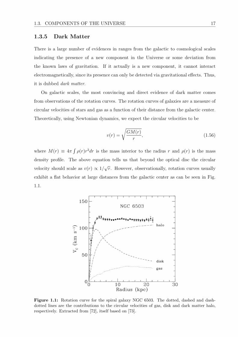
On galactic scales, the most convincing and direct evidence of dark matter comes
from observations of the rotation curves. The rotation curves of galaxies are a measure of
circular velocities of stars and gas as a function of their distance from the galactic center.
Theoretically, using Newtonian dynamics, we expect the circular velocities to be
v(r) =
√GM(r)
r, (1.56)
where M(r) ≡ 4π∫ρ(r)r2dr is the mass interior to the radius r and ρ(r) is the mass
density profile. The above equation tells us that beyond the optical disc the circular
velocity should scale as v(r) ∝ 1/√r. However, observationally, rotation curves usually
exhibit a flat behavior at large distances from the galactic center as can be seen in Fig.
1.1.
Figure 1.1: Rotation curve for the spiral galaxy NGC 6503. The dotted, dashed and dash-dotted lines are the contributions to the circular velocities of gas, disk and dark matter halo,respectively. Extracted from [72], itself based on [73].
18 CHAPTER 1. INTRODUCTION TO COSMOLOGY
Actually, the first indication of dark matter was obtained by Zwicky in 1933 [74].
Studying the Coma cluster he inferred a mass-to-light ratio of 400 solar masses per solar
luminosity, two orders of magnitude greater than observed in the solar neighborhood. The
mass of a galaxy cluster can be determined in several ways: applying the virial theorem
to the observed distribution of radial velocities, by weak gravitational lensing, and from
the X-ray emitted by the hot gas in the cluster. All of these measurements are consistent
with Ωm ∼ 0.2− 0.3 [75–77].
Finally, on cosmological scales, the anisotropies of the cosmic microwave background
(CMB) provide stringent constraints on the abundance of baryons and dark matter in the
Universe as placed by the Wilkinson Microwave Anisotropy Probe (WMAP) data. Recent
determinations give Ωdm0 = 0.228± 0.013 [68].
All of these evidences show that there must be in the Universe a component that
contributes with around 25% of the critical energy density. Since baryons contribute with
only 5%, this component must be nonbaryonic. Because it does not interact electromag-
netically the first guess would be neutrinos. However, from (1.55) and the upper limit on
the neutrino mass mν < 2.05eV [78], we have
Ωνh2 ≤ 0.07, (1.57)
which means that there are not enough neutrinos to be the dominant component of dark
matter. Thus, dark matter must really be a new component.
1.3.6 Dark Energy
Observations of anisotropies in the CMB have shown that the geometry of the spatial
section is very close to a flat one [79–82]. Actually, we also expect this theoretically from
inflationary scenarios in the early Universe [60]. This means that the total energy density
should be equal to the critical density. However, summing the contributions of all the
components described so far, we obtain that they contribute with around 30% of the
critical density. Thus, there is a lack of 70% in the energy content of the Universe.
Using the luminosity distance (1.29) we can find the apparent magnitude m of an
1.3. COMPONENTS OF THE UNIVERSE 19
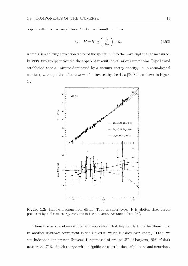
object with intrinsic magnitude M . Conventionally we have
m−M = 5 log
(dL
10pc
)+K, (1.58)
whereK is a shifting correction factor of the spectrum into the wavelength range measured.
In 1998, two groups measured the apparent magnitude of various supernovae Type Ia and
established that a universe dominated by a vacuum energy density, i.e. a cosmological
constant, with equation of state ω = −1 is favored by the data [83, 84], as shown in Figure
1.2.
Figure 1.2: Hubble diagram from distant Type Ia supernovae. It is plotted three curvespredicted by different energy contents in the Universe. Extracted from [60].
These two sets of observational evidences show that beyond dark matter there must
be another unknown component in the Universe, which is called dark energy. Then, we
conclude that our present Universe is composed of around 5% of baryons, 25% of dark
matter and 70% of dark energy, with insignificant contributions of photons and neutrinos.
20 CHAPTER 1. INTRODUCTION TO COSMOLOGY
Nowadays, the best model explaining the data is the ΛCDM , with cold dark matter
(CDM) and where dark energy is the cosmological constant Λ.
The ΛCDM model is the simplest one that fits the data. However, it suffers of two
theoretical problems. The first occurs when we try to associate the cosmological constant
with the vacuum energy density. In quantum field theory, we generally introduce a cut
off on the energy beyond which our theory cannot describe the physics. If we introduce
this cut off at the Planck reduced mass MPl = (8πG)−1/2 = 2.436 × 10¹⁸GeV [85], the
vacuum energy density will be given by ρvac ∼ M4Pl ∼ 1073(GeV )4. On the other hand,
the energy density of dark energy today is ρΛ = 3M2PlH
20 ΩΛ ∼ 10−47(GeV )4. Thus, there
is a difference of 120 orders of magnitude, which is known as the cosmological constant
problem.
The second problem arises when we consider the evolution of the components in the
Universe. As we already saw, the non-relativistic matter (baryons and dark matter)
scales as ρm ∝ a−3, radiation scales as ρr ∝ a−4 and the cosmological constant has a
density ρΛ = constant. Therefore, each component scales in a very different way. But,
as mentioned above, matter and dark energy have the same order of magnitude today.
Thus, the question arise: “why matter and dark energy have the same order of magnitude
exactly now in the whole history of the Universe?”. This is called the coincidence problem.
These difficulties in the ΛCDM model have motivated the search for new models of
dark energy. In conclusion we observe that both dark matter and dark energy have no
explanation in the standard model of particle physics.

Chapter 2
Cosmological Perturbations
The description of the Universe was, up to now, performed considering it as homoge-
neous and isotropic, as described by the cosmological principle. However, the structures
around us imply that at some point we have to break these assumptions and introduce
inhomogeneities and anisotropies in our model. Because on large scales the cosmological
principle leads to correct results, we shall do that using perturbation theory.
2.1 Perturbed Metric
The metric of a flat FLRW universe with small perturbations can be written as
ds2 =[
(0)gµν + δgµν(xγ)]dxµdxν , (2.1)
where (0)gµν corresponds to the unperturbed part and |δgµν | |(0)gµν |. Using the confor-
mal time (1.17), the most general components of the metric tensor are given by [86]
g00 = −a2(1 + 2ψ), (2.2)
g0i = a2(B,i +Si), (2.3)
gij = a2 [(1 + 2φ)δij +DijE + Fi,j +Fj,i +hij] , (2.4)
where the perturbations are introduced by the scalar functions ψ, B, φ and E; the diver-
gence free vectors Si and Fi; and a traceless and transverse tensor hij. Here the comma
means differentiation with respect to the respective spatial index, e.g. B,i = ∂B/∂xi. We
21
22 CHAPTER 2. COSMOLOGICAL PERTURBATIONS
also define
Dij =
(∂i∂j −
1
3δij∇2
). (2.5)
From the three types of perturbations, the scalars are the most important in cosmology
because they present gravitational instability and can lead to structure formation in the
Universe. The vector perturbations are responsible for rotational motions of the fluid and
decay very quickly. Finally, tensor perturbations describe gravitational waves, but in the
linear approximation they do not induce perturbations in the perfect fluid. Moreover,
the decomposition theorem [60, 86] states that these three types of perturbations evolve
independently. Thus, in this work, we will only be interested in scalar perturbations. In
this case the metric becomes
ds2 = a2[−(1 + 2ψ)dη2 + 2∂iBdηdx
i + (1 + 2φ)δijdxidxj +DijEdx
idxj]. (2.6)
Given a coordinate transformation
xµ → xµ = xµ + ξµ, (2.7)
where ξµ ≡ (ξ0, ξi⊥+ ζ ′i) are infinitesimally small functions of space and time, the metric
tensor has its components changed by
gµν(xρ) =
∂xγ
∂xµ∂xδ
∂xνgγδ(x
ρ) ≈ (0)gµν(xρ) + δgµν − (0)gµδξ
δ,ν − (0)gγνξγ,µ , (2.8)
at first order in δg and ξ. The new coordinate system also allows to split the metric into
a background and a perturbed part
gµν(xρ) = (0)gµν(x
ρ) + δgµν , (2.9)
where (0)gµν(xρ) is the Friedmann metric in the new coordinates. On the other hand,
expanding the background part of (2.1) in a Taylor series around the coordinates x, we
have
(0)gµν(xρ) ≈ (0)gµν(x
ρ) − (0)gµν ,γ ξγ . (2.10)
Therefore, comparing Eqs. (2.8) and (2.9) and also using Eq. (2.10), we obtain the gauge
2.1. PERTURBED METRIC 23
transformation law
δgµν → δgµν = δgµν − (0)gµν ,γ ξγ − (0)gµδξ
δ,ν − (0)gγνξγ,µ . (2.11)
Using the gauge transformation law (2.11), the metric (2.6) has its components changed
as
ψ = ψ − 1
a(aξ0)′, (2.12)
B = B − ζ ′ + ξ0, (2.13)
φ = φ− 1
6∇2E − a′
aξ0, (2.14)
E = E − 2ζ. (2.15)
Here a prime means the derivative with respect to the conformal time. The coordinate
transformation (2.7) is completely arbitrary, then we can choose ξ0 and ζ freely. Thus, the
above transformations of the metric components show we can choose ξ0 and ζ appropri-
ately in order to eliminate two of the four functions ψ, B, φ and E. Therefore, there are
just two physical perturbations. Combining equations (2.12)-(2.15), we can construct two
gauge-invariant functions which span the two-dimensional space of physical perturbations
Ψ = ψ − 1
a
[(−B +
E ′
2
)a
]′, (2.16)
Φ = φ− 1
6∇2E +
a′
a
(B − E ′
2
). (2.17)
Instead of working with gauge-invariant functions, we can impose two conditions on
the coordinate transformation, which is equivalent to a gauge choice. In particular, the
conformal-Newtonian gauge is obtained with coordinates ξ0 and ζ such that B = E = 0.
Another gauge, widely used in the literature, is the synchronous gauge. It corresponds
to the gauge choice ψ = B = 0. However, unlike the conformal-Newtonian gauge, the
synchronous gauge does not fix the coordinates uniquely. If the conditions ψ = B = 0 are
satisfied in a coordinate system xµ ≡ (η, ~x), they will also be satisfied in any coordinate
system xµ given by
η = η +C1(xj)
a, xi = xi + C1,i (x
j)
∫dη
a+ C2,i (x
j), (2.18)

24 CHAPTER 2. COSMOLOGICAL PERTURBATIONS
where C1(xj) and C2(xj) are arbitrary functions of the spatial coordinates.
Equations (2.16) and (2.17) allow to relate the gauge-invariant perturbations with the
perturbations in a particular gauge. Thus, if we know a solution for perturbations with
gauge-invariant variables, or using the conformal-Newtonian gauge, we can transform it
into the synchronous gauge without needing to solve the Einstein equations again.
2.2 Einstein Equations
Now we know the components of the perturbed metric tensor. We can thus obtain their
evolution using the Einstein equations (1.5). Assuming the perturbations are small we
can expand them in a Taylor series. Thus, as we did to the metric tensor, it is possible
to split the Einstein tensor Gµν and the energy-momentum tensor T µν into background
and perturbed parts: Gµν = (0)Gµ
ν + δGµν and T µν = (0)T µν + δT µν . The zeroth order
terms correspond to the homogeneous and isotropic background and the others give us
the perturbed Einstein equations
δGµν = 8πGδT µν . (2.19)
The geometric part of the Einstein equations (2.19) can be solved following the same
procedure adopted in the last chapter. Thus, using the perturbed metric (2.6) in the
conformal-Newtonian gauge and keeping only first-order terms, we obtain
δG00 = 2a−2
[3H (HΨ− Φ′) +∇2Φ
], (2.20)
δG0i = 2a−2 (Φ′ −HΨ) ,i , (2.21)
δGij = 2a−2
[(H2 + 2H′
)Ψ +HΨ′ − Φ′′ − 2HΦ′
]δij +
a−2[∇2 (Ψ + Φ) δij − (Ψ + Φ) ,ij
]. (2.22)
Here we defined the conformal Hubble parameter H ≡ 1adadη
= Ha and from Eqs. (2.16)
and (2.17) we see that Ψ = ψ and Φ = φ in this gauge.
From equations (2.20)-(2.22), we observe that the Einstein equations (2.19) turn out
to be a set of linear partial differential equations. If we Fourier expand all perturbation
2.3. BOLTZMANN EQUATION 25
quantities
θ(~x, η) =
∫d3k
(2π)3ei~k·~xθk(η), (2.23)
where θ denotes a generic perturbation and the subscript k represents a Fourier mode for
each wavenumber k, the resulting Fourier amplitudes obey ordinary differential equations.
Thus, working in the Fourier space makes things easier. Furthermore, the Fourier modes
θk evolve independently in the linear regime. Therefore, instead of solving an infinite
number of coupled equations, we can solve for one k-mode at a time. In practice, each
perturbation quantity θ and its derivatives can be substituted as
θ(~x, η) → ei~k·~xθ(η), (2.24)
~∇θ(~x, η) → iei~k·~x~kθ(η), (2.25)
∇2θ(~x, η) ≡ ∇i∇iθ(~x, η) → −ei~k·~xk2θ(η), (2.26)
where we are omitting the subscript k to simplify the notation.
The Einstein equations are a set of 16 equations. However, the symmetries in the
indices µ, ν reduce the number of independent equations to 10. Only two of the four scalar
functions in the metric (2.6) represent physical states. Thus, choosing the conformal-
Newtonian gauge, we just need two Einstein equations to obtain the evolution of the
functions Ψ and Φ. We choose the time-time component of the Einstein equations (2.19)
δG00 =
2
a2
[3H(HΨ− Φ′
)− k2Φ
]= 8πGδT 0
0 (2.27)
and the longitudinal traceless projection of the space-space components
(kik
j − 1
3δji
)δGi
j =2
3a2k2(Ψ + Φ) = 8πG
(kik
j − 1
3δji
)δT ij . (2.28)
These equations were written in the Fourier space and we defined the unit direction
wavevector ki = ki, which satisfies δij kikj = 1.
2.3 Boltzmann Equation
To solve the Einstein equations (2.27) and (2.28) we need the first-order components of
the energy-momentum tensor. This could be obtained using the hydrodynamic equations
26 CHAPTER 2. COSMOLOGICAL PERTURBATIONS
as in the homogeneous and isotropic case. However, those equations can be obtained
by the first moments of the Boltzmann equation, which means that it is more general.
Furthermore, the radiation description is made using fluctuations of the temperature, and
the Boltzmann formalism is more natural in this case.
The Boltzmann equation formalizes the statement that the variation in the distribution
of some species is equal to the difference between the rates of ingoing and outgoing
particles of that species. In its differential form, the Boltzmann equation is
df
dt= C[f ], (2.29)
where f is the distribution function and C[f ] is a functional of the distribution function,
which establishes all possible collision terms of the particle of interest. In general, f is a
function of the spacetime point xµ = (t, ~x) and also of the four-dimensional momentum
vector in comoving frame
P µ ≡ dxµ
dλ, (2.30)
where λ parametrizes the particle’s path. The four-vector P µ is related to the physical
momentum four-vector pµ by P µ = ∂xµ
∂xνpν , with xν in the physical frame.
In order to calculate the perturbed energy-momentum tensor, we develop below the
Boltzmann equation for each component in the Universe.
2.3.1 Photons
Photons satisfy the energy-momentum relation
P 2 ≡ gµνPµP ν = −(1 + 2Ψ)(P 0)2 + gijP
iP j = −(1 + 2Ψ)(P 0)2 + p2 = 0, (2.31)
where we used the metric (2.6) in the conformal-Newtonian gauge passing to the cosmic
time and p2 is the generalized magnitude of the momentum. The above relation allows
us to express P 0 in terms of p. Thus, there are only three independent components of
the four-dimensional momentum vector. Then, we can expand the total time derivative
of f in the Boltzmann equation (2.29) considering only the momentum magnitude p and
2.3. BOLTZMANN EQUATION 27
angular direction pi = pi:
df
dt=∂f
∂t+∂f
∂xi· dx
i
dt+∂f
∂p· dpdt
+∂f
∂pi· dp
i
dt, (2.32)
where δij pipj = 1.
Let us begin to solve equation (2.32). The last term does not contribute at first order
in perturbation theory. In fact, the zeroth order part of f depends only on p, which
means ∂f/∂pi is nonzero only in a perturbed level. In the same way, a photon moves in a
straight line in the absence of the potentials Ψ and Φ, therefore, dpi/dt is also a perturbed
quantity. Thus, the last term of (2.32) must be of second order.
Using the definition of the comoving energy-momentum vector (2.30), we obtain
dxi
dt=dxi
dλ
dλ
dt=P i
P 0. (2.33)
From (2.31) the time-component of P µ is given by
P 0 =p√
1 + 2Ψ= p(1−Ψ), (2.34)
where the last equality is valid at first order. On the other hand, the spatial component
is proportional to the unit direction vector pi
P i ≡ |P |pi. (2.35)
Plugging (2.35) in the definition of the spatial magnitude, we find
p2 ≡ gijPiP j = a2(1 + 2Φ)(δij p
ipj)P 2 = a2(1 + 2Φ)P 2, (2.36)
which gives |P | = p(1 − Φ)/a at first order. Therefore, combining equations (2.34) and
(2.35), we havedxi
dt=
1− Φ + Ψ
api. (2.37)
The next term we need to evaluate is dp/dt. This factor can be calculated from the
time component of the geodesic equation dP 0/dλ = −Γ0µνP
µP ν in a simple, although
28 CHAPTER 2. COSMOLOGICAL PERTURBATIONS
tedious, way [60]. Here we just show the final result
dp
dt= −p
(H +
∂Φ
∂t+pi
a
∂Ψ
∂xi
). (2.38)
Combining the terms obtained so far, the left hand side of the Boltzmann equation for
photons yieldsdf
dt=∂f
∂t+pi
a
∂f
∂xi− p∂f
∂p
(H +
∂Φ
∂t+pi
a
∂Ψ
∂xi
), (2.39)
where we neglected the product of ∂f/∂xi and either Ψ or Φ because they are second-order
terms.
Photons in a homogeneous and isotropic distribution with an equilibrium temperature
T obey the Bose-Einstein statistics given by equation (1.40). There, T is a function
of time only. To describe perturbations about this distribution, we have to introduce
inhomogeneities, so that it must have an ~x dependence, and anisotropies, which means
a dependence with the direction of propagation p. Thus, for photons, the distribution
function is given by
f(t, ~x, p, p, ) =
exp
[p
T (t)[1 + Θ(t, ~x, p)]
]− 1
−1
, (2.40)
where T (t) is the zero-order temperature and Θ ≡ δT/T characterizes the perturbation to
the distribution function. Here we have assumed that Θ does not depend on the magnitude
p, which is a valid assumption since in a Compton scattering p is approximately conserved.
Expanding up to first order,
f = f (0) + T∂f (0)
∂TΘ = f (0) − p∂f
(0)
∂pΘ. (2.41)
Plugging Eq. (2.41) into Eq. (2.39) and collecting terms of similar order, at zeroth order
we find the background equations for the number and energy conservation from the first
moments of the Boltzmann equation. Finally, the first-order terms result in
df (1)
dt= −p∂f
(0)
dp
[∂Θ
∂t+pi
a
∂Θ
∂xi+∂Φ
∂t+pi
a
∂Ψ
∂xi
]. (2.42)
The last step necessary to calculate the Boltzmann equation for photons is the collision
2.3. BOLTZMANN EQUATION 29
term. Photons interact with electrons through the Compton scattering
e−(~q) + γ(~p)↔ e−(~q ′) + γ(~p ′), (2.43)
where the momentum of each particle is indicated. To obtain the effect of the Compton
scattering in the distribution function of photons with momentum ~p, we must sum the
contributions of all the other momenta to the collision term [60]
C[f(~p)] =1
p
∫d3q
(2π)32Ee(q)
∫d3q′
(2π)32Ee(q′)
∫d3p′
(2π)32E(p′)|M|2(2π)4
× δ3[~p+ ~q − ~p ′ − ~q ′]δ[E(p) + Ee(q)− E(p′)− Ee(q′)]× fe(~q ′)f(~p ′)− fe(~q)f(~p) .
(2.44)
Some explanation about the collision term is fruitful here. First we note that in the
Boltzmann equation (2.29) we considered the total time derivative of the distribution f .
However, general relativity requires derivatives with respect to the affine parameter λ,
dfdλ
= dtdλ
dfdt
= P 0 dfdt
. At first order this introduces the factor 1p
in front of the integrals.
Actually, the integrals are over the four-momentum vectors and the factors of 2E come
from the integration over the time component. M is the scattering amplitude of the
process in question, which can be found using the Feynman rules. The delta functions
arise from conservation of energy and momentum. Finally, the last terms count the
number of particles with the given momenta 1.
At the epochs of interest the energies are the relativistic limit for photons E(p) = p
and the non-relativistic limit for electrons Ee(q) = me + q2/(2me) ≈ me. Thus, we can
use the three-dimensional delta function to eliminate the integral over ~q ′
C[f(~p)] =π
4m2ep
∫d3q
(2π)3
∫d3p′
(2π)3p′|M|2 × δ[p+
q2
2me
− p′ − (~q + ~p− ~p ′)2
2me
]
× fe(~q + ~p− ~p ′)f(~p ′)− fe(~q)f(~p) . (2.45)
For non-relativistic Compton scattering very little energy is transferred Ee(q) − Ee(~q +
~p − ~p ′) ≈ (~p ′−~p)·~qme
, which holds since ~q is much larger than ~p and ~p ′. In this limit, the
scattering is nearly elastic p′ ≈ p. As the change in the electron energy is small, it makes
1We should include additional factors of 1 + f and 1− fe for stimulated emission and Pauli blocking,respectively. However, at first order these terms can be neglected.
30 CHAPTER 2. COSMOLOGICAL PERTURBATIONS
sense to expand the final electron kinetic energy (~q + ~p − ~p ′)2/(2me) around its zeroth
order value q2/(2me). Therefore, we can make the formal expansion in the delta function
δ[p+q2
2me
− p′ − (~q + ~p− ~p ′)2
2me
] ≈ δ(p− p′)
+ [Ee(q′)− Ee(q)]
∂δ[p+ Ee(q)− p′ − Ee(q′)]∂Ee(q′)
∣∣∣∣Ee(q)=Ee(q′)
= δ(p− p′) +(~p− ~p ′) · ~q
me
∂δ(p− p′)∂p′
. (2.46)
Using this expansion and fe(~q + ~p− ~p ′) ≈ fe(~q), we obtain
C[f(~p)] =π
4m2ep
∫d3q
(2π)3fe(~q)
∫d3p′
(2π)3p′|M|2
×δ(p− p′) +
(~p− ~p ′) · ~qme
∂δ(p− p′)∂p′
× f(~p ′)− f(~p) . (2.47)
The amplitude for Compton scattering can be found using the Feynman rules [87]
|M|2 = 12πσTm2e(ε · ε ′), (2.48)
where σT is the Thomson cross section, ε and ε ′ are the polarization vectors of the initial
and final photons, respectively. For simplicity, we average over all polarizations and
angular dependence which results in a constant amplitude
|M|2 = 8πσTm2e. (2.49)
Thus, using this amplitude and the expansion of the distribution function (2.41), the
collision term can be written as
C[f(~p)] =2π2neσT
p
∫d3p′
(2π)3p′×δ(p− p′) + (~p− ~p ′) · ~vb
∂δ(p− p′)∂p′
×f (0)(~p ′)− f (0)(~p)− p′∂f
(0)
∂p′Θ(p ′) + p
∂f (0)
∂pΘ(p)
, (2.50)
where we did the integrals over momentum ~q using the number density definition (1.37)
and we define the velocity as
vi ≡ g∗n
∫d3p
(2π)3fppi
E. (2.51)
2.3. BOLTZMANN EQUATION 31
The spin degeneracy g∗ can be incorporated into the phase space distribution f .
To solve the integral over ~p ′ in Eq. (2.50), we split the radial and angular parts of the
differential d3p′. Then, keeping only first-order terms in perturbations, the integral over
the solid angle yields
C[f(~p)] =neσTp
∫ ∞0
dp′p′δ(p− p′)
[−p′∂f
(0)
∂p′Θ0 + p
∂f (0)
∂pΘ(p)
]+~p · ~vb
∂δ(p− p′)∂p′
[f (0)(p′)− f (0)(p)
], (2.52)
where we define the multipoles
Θl ≡1
(−i)l
∫ 1
−1
dµ
2Pl(µ)Θ(µ), (2.53)
such that Pl is the Legendre polynomial of order l and instead of the unit vector p, we
used the direction cosine
µ ≡~k · pk. (2.54)
Finally, the p′ integral can be done in the first line of Eq. (2.52) with the delta function
and in the second line integrating by parts, the result is [60]
C[f(~p)] = −p∂f(0)
∂pneσT [Θ0 −Θ(p) + p · ~vb] , (2.55)
where ne is the electron density and ~vb is the velocity of the electrons, which is associated
with the baryons.
At last the first-order Boltzmann equation (2.29) for photons can be obtained equating
Eq. (2.42) and Eq. (2.55)
∂Θ
∂t+pi
a
∂Θ
∂xi+∂Φ
∂t+pi
a
∂Ψ
∂xi= neσT [Θ0 −Θ(p) + p · ~vb] . (2.56)
As usual we assume the fluid to be irrotational, which means we can write vib = vbki/k.
Thus, passing to the conformal time and Fourier space we obtain
Θ′ + ikµΘ + Φ′ + ikµΨ = −τ ′[Θ0 − Θ(p) + µvb
], (2.57)

32 CHAPTER 2. COSMOLOGICAL PERTURBATIONS
where we defined the optical depth
τ ≡∫ η0
η
neσTadη. (2.58)
When deriving Eq. (2.57) we use a constant amplitude given by (2.49). Actually,
the Compton scattering has an angular dependence and it also couples the temperature
field to the strength of the polarization field ΘP . The general expression can be obtained
following the same procedure we did, but using the complete amplitude (2.48). The
answer is [60]
Θ′ + ikµΘ + Φ′ + ikµΨ = −τ ′[Θ0 − Θ + µvb −P2(µ)
2Π], (2.59)
where Π = Θ2 + ΘP2 + ΘP0. ΘP0 and ΘP2 are the monopole and quadrupole of the
polarization field, which satisfies
Θ′P + ikµΘP = −τ ′[−ΘP +1− P2(µ)
2Π]. (2.60)
The above equations show that even if we are interested only in the temperature field, it
is influenced by the polarization field.
2.3.2 Baryons
The formalism presented in the last subsection can be used to obtain the Boltzmann
equation for any constituent in the Universe. We now move to consider the behavior of
massive particles, for which we have
P 2 = gµνPµP ν = −m2. (2.61)
Defining the energy
E ≡√p2 +m2, (2.62)
where p2 is the same as in equation (2.36), the four-momentum of a massive particle is
given by
P µ =
[(1−Ψ)E,
1− Φ
appi]. (2.63)

2.3. BOLTZMANN EQUATION 33
Instead of the momentum p, massive particles must be described by the energy E.
Therefore, the left hand side of the Boltzmann equation (2.29) is expanded as
df
dt=∂f
∂t+∂f
∂xi· dx
i
dt+∂f
∂E· dEdt
+∂f
∂pi· dp
i
dt. (2.64)
Following the same steps as for the case of photons, we can obtain the coefficients dxi/dt
and dE/dt such that Eq. (2.64) can be rewritten as
df
dt=∂f
∂t+pi
a
p
E
∂f
∂xi− p ∂f
∂E
(Hp
E+p
E
∂Φ
∂t+pi
a
∂Ψ
∂xi
). (2.65)
Once again we neglected the last term in Eq. (2.64) as it does not contribute at first order.
The main difference of this equation to the photon case is the presence of factors p/E,
which arise from the energy-momentum constraint. The massless case can be recovered
from Eq. (2.65) with E = p.
When we considered photons, to complete the left hand side of the Boltzmann equa-
tion, we needed the knowledge of the distribution function. For massive particles, the
treatment can be simplified if they are nonrelativistic. In this case, we do not need a
detailed information about the distribution function, all we need is to take moments of
the Boltzmann equation taking into account that terms second-order in v = p/E must be
neglected because of the nonrelativistic behavior.
The zeroth moment is obtained integrating the Boltzmann equation as
∫d3p
(2π)3
df
dt=
∂
∂t
∫d3p
(2π)3f +
1
a
∂
∂xi
∫d3p
(2π)3fppi
E
−[H +
∂Φ
∂t
] ∫d3p
(2π)3
∂f
∂E
p2
E− 1
a
∂Ψ
∂xi
∫d3p
(2π)3
∂f
∂Eppi. (2.66)
From the definitions (1.37) and (2.51), the first two terms of the right hand side of
equation (2.66) can be written in terms of the number density and velocity, respectively
2. To integrate the third term of the r.h.s. of Eq. (2.66) we observe that dE/dp = p/E,
thus
∫d3p
(2π)3
∂f
∂E
p2
E=
∫d3p
(2π)3p∂f
∂p=
∫dΩ
(2π)3
∫ ∞0
dpp3∂f
∂p= −3
∫dΩ
(2π)3
∫ ∞0
dp p2f = −3n,
(2.67)
2The spin degeneracy g∗ can be incorporated in the phase space distribution f .

34 CHAPTER 2. COSMOLOGICAL PERTURBATIONS
where in the third step we integrated by parts. The last term of (2.66) does not contribute
at first order since the integral over the direction vector is null at zeroth order and that
integral multiplies a metric perturbation, thus this term is at least of second order. Finally,
we obtain ∫d3p
(2π)3
df
dt=∂n
∂t+
1
a
∂(nvi)
∂xi+ 3
(H +
∂Φ
∂t
)n. (2.68)
The above result for the zeroth moment of the Boltzmann equation has introduced
two unknown variables: n and vi. Thus, we need one more equation to close the system.
This additional equation can be obtained taking the first moment
∫d3p
(2π)3
ppj
E
df
dt=
∂
∂t
∫d3p
(2π)3fppj
E+
1
a
∂
∂xi
∫d3p
(2π)3fp2pipj
E2
−[H +
∂Φ
∂t
] ∫d3p
(2π)3
∂f
∂E
p3pj
E2− 1
a
∂Ψ
∂xi
∫d3p
(2π)3
∂f
∂E
p2pipj
E. (2.69)
The first term on the r.h.s. can be identified with the partial time derivative of nvj.
The second one is neglected at first order since it depends on (p/E)2. To calculate the
last terms, we follow the same procedure used in Eq. (2.67). Therefore, keeping only
first-order terms, the first moment of the Boltzmann equation is
∫d3p
(2π)3
ppj
E
df
dt=∂(nvj)
∂t+ 4Hnvj +
n
a
∂Ψ
∂xj. (2.70)
An interesting fact can be observed by taking moments of the Boltzmann equation: the
lth moment depends on the (l + 1)th moment. Thus, in principle, they constitute an
infinite hierarchy of equations. However, as we are considering nonrelativistic particles,
we neglected terms of second order and higher in (p/E) which correspond to the higher
moments. Therefore, Eqs. (2.68) and (2.70) form a closed system for n and vi.
Until now we restricted the analysis to the left hand side of the Boltzmann equation.
The results presented in equations (2.68) and (2.70) are general for any massive and
nonrelativistic component in the Universe. To proceed further let us restrict the study to
the case of baryons.
Electrons and protons are coupled by Coulomb scattering whose rate is much larger
than the expansion rate at all epochs of interest. Because of this tight coupling, electrons
2.3. BOLTZMANN EQUATION 35
and protons have the same overdensities
ρe − ρ(0)e
ρ(0)e
=ρp − ρ(0)
p
ρ(0)p
≡ δb (2.71)
and velocities
~ve = ~vp ≡ ~vb. (2.72)
Besides the Coulomb scattering, baryons interact with photons through the Compton
scattering. Thus, the unintegrated Boltzmann equation for baryons is given by
dfb(t, ~x, ~q)
dt= 〈ceγ〉pp′q′ , (2.73)
where 〈ceγ〉pp′q′ represents the Compton collision term, as in Eq. (2.44), and the subscripts
represent which momenta are being integrated. In principle, the collision term should have
an additional term account for the proton-photon Compton scattering, however, the cross
section for this process is much smaller than the electron-photon scattering and can be
ignored. We are also considering a simplified model with all electrons ionized.
To solve Eq. (2.73) we first take the zeroth moment integrating in the electron mo-
mentum ~q. Thus, using Eq. (2.68) we obtain
∂nb∂t
+1
a
∂(nbvib)
∂xi+ 3
(H +
∂Φ
∂t
)nb = 〈ceγ〉pp′q′q . (2.74)
The collision term in the right hand side vanishes since the integration is symmetric under
the interchange of p↔ p′ and q ↔ q′ while it is antisymmetric in the distribution function
factors. The number density can be split into a background part and a perturbed part as
nb = n(0)b [1 + δb]. Thus, collecting the zeroth order and first-order terms, and passing to
conformal time and Fourier space, the perturbed part gives us
δ′b + ikvb + 3Φ′ = 0. (2.75)
The second equation, which describes the evolution of the velocity field, is obtained
taking the first moment of Eq. (2.73). In Eq. (2.70) we found the first moment of the
left-hand side of the Boltzmann equation. There we first multiplied by ~p/E and then
integrated. For baryons we multiply Eq. (2.73) by the momentum ~q instead of ~q/E. This
36 CHAPTER 2. COSMOLOGICAL PERTURBATIONS
will produce the same result as (2.70) except for a factor of mb
mb∂(nbv
jb)
∂t+ 4Hmbnbv
jb +
mbnba
∂Ψ
∂xj=⟨ceγq
j⟩pp′q′q
. (2.76)
Using the conservation of the total momentum ~q + ~p, we have that 〈ceγ~q〉pp′q′q =
−〈ceγ~p〉pp′q′q. Passing to Fourier space and multiplying Eq. (2.76) by kj, the right-hand
side becomes −〈ceγpµ〉pp′q′q. In equation (2.55), we already computed 〈ceγ〉p′q′q, thus we
just need to multiply that result by pµ and integrate over all ~p,
−〈ceγpµ〉pp′q′q = neσT
∫d3p
(2π)3p2∂f
(0)
∂pµ[Θ0 − Θ(µ) + µvb
]= neσT
∫ ∞0
dp
2π2p4∂f
(0)
∂p
∫ 1
−1
dµ
2µ[Θ0 − Θ(µ) + µvb
]. (2.77)
In the second line we split the integration over ~p into a radial part and an angular part.
The integral over the radial part p can be made integrating by parts similar to Eq.(2.67),
the result is −4ργ. The first term in the µ-integration vanishes, the second term is the
dipole component of Θ and the last term reduces to vb/3. Therefore, collecting these
results in Eq. (2.76) and switching to conformal time, we obtain
v′b +a′
avb + ikΨ = τ ′
4ργ3ρb
[3iΘ1 + vb
]. (2.78)
2.3.3 Neutrinos
Equation (2.59) can be extended to massless neutrinos. They obey a similar equation
without a collision term,
N ′ + ikµN + Φ′ + ikµΨ = 0, (2.79)
where N is the perturbation in the neutrino temperature. On the other hand, if neutrinos
are massive, the left-hand side of the Boltzmann equation will be given by Eq. (2.65).
However, unlike the baryon case, neutrinos are relativistic particles, then we cannot ne-
glect terms of order (p/E)2 and higher, we have to take into account the whole hierarchy
of moments. A discussion about massive neutrinos can be found in [88].

2.3. BOLTZMANN EQUATION 37
2.3.4 Dark Matter
Cold dark matter behaves like baryons. However, it does not interact electromagnetically,
then the perturbations are not affected by a collision term 3. Thus, the density contrast
of cold dark matter obeys an equation identical to (2.75)
δ′c + ikvc + 3Φ′ = 0 (2.80)
and the velocity equation is similar to (2.78) without a collision term
v′c +a′
avc + ikΨ = 0. (2.81)
We observe that to obtain Eqs. (2.80) and (2.81) we use the Boltzmann equation, how-
ever, cold dark matter always behaves like a fluid, which means that it can be described
completely by the energy-momentum tensor Tµν . Thus, we could obtain the evolution
equations above using the conservation of the energy-momentum tensor as we did in the
homogeneous case.
2.3.5 Energy-Momentum Tensor
Now that we know the equations governing the evolution of perturbations in the compo-
nents of the Universe, we are in position to complete the Einstein equations (2.27) and
(2.28) with the perturbed energy-momentum tensor. In general, the energy-momentum
tensor of a fluid with a distribution function f(t, ~x, ~p) is given by
T µν (t, ~x) = g∗
∫d3p
(2π)3
pµpνE
f(t, ~x, ~p). (2.82)
Remember that the Einstein equations take into account the contributions of all species
in the Universe, thus from the time-time component of (2.82), we obtain
T 00 = −
∑all species i
g∗i
∫d3p
(2π)3Ei(p)fi(t, ~x, ~p). (2.83)
The distribution functions above consist in a background part and a perturbed part.
For nonrelativistic particles, the integral produces −ρi(1 + δi), while for relativistic ones,
3In the next chapter we will extend this model assuming an interaction in the dark sector.
38 CHAPTER 2. COSMOLOGICAL PERTURBATIONS
the integral can be done using the expansion (2.41). Considering only the first-order
perturbations, the Einstein equation (2.27) results
k2Φ + 3a′
a
(Φ′ − Ψ
a′
a
)= 4πGa2
[ρcδc + ρbδb + 4ργΘ0 + 4ρνN0
], (2.84)
where N0 is the monopole term of the neutrino temperature perturbations.
The second Einstein equation (2.28) needs the longitudinal traceless projection of the
space-space energy-momentum tensor
(kik
j − 1
3δji
)T ij =
∑all species i
g∗i
∫d3p
(2π)3p2µ
2 − 1/3
Ei(p)fi(t, ~x, ~p). (2.85)
We observe that the factor µ2−1/3 is equal to 2/3P2(µ), where P2(µ) is the second Legen-
dre polynomial. Therefore, the integral picks out the quadrupole part of the distributions.
We already saw that nonrelativistic particles do not contribute to the second moment and
higher, thus only photons and neutrinos must be taken into account. For example, let us
calculate the integral in the case of photons:
− 2
∫dp
2π2p4∂f
(0)
∂p
∫ 1
−1
dµ
2
2P2(µ)
3Θ(µ) =
4Θ2
3
∫dp
2π2p4∂f
(0)
∂p= −8ργΘ2
3. (2.86)
Finally, combining (2.28) and (2.85) we obtain the second Einstein equation
k2(Φ + Ψ) = −32πGa2[ργΘ2 + ρνN2
]. (2.87)
We emphasize that, in principle, we should have a term for perturbations in the dark
energy in the Einstein equations above. However, until now, we consider it to be smooth
and important only very recently as described by the cosmological constant model.
2.4 Initial Conditions
Equations (2.59), (2.60), (2.75), (2.78), (2.79), (2.80), (2.81), (2.84) and (2.87) form a
system of nine first-order differential equations. To solve them we need a set of nine
initial conditions. However, in the early Universe, we can relate all perturbation variables
to the gravitational potential Φ, such that we will actually need just one initial condition.

2.4. INITIAL CONDITIONS 39
Considering times so early that for all k-modes of interest kη 1, we can neglect
all terms in the Boltzmann equations multiplied by k. This condition means that on
early times all perturbations of interest had wavelengths much larger than the distance
of causal contact. Thus, an observer within the causal horizon sees a uniform sky, which
means that higher multipoles, e.g. Θ1, Θ2, ..., are much smaller than the monopole term.
Therefore, using these considerations, equations (2.59), (2.79), (2.75) and (2.80) can be
written as
Θ′0 + Φ′ = 0, (2.88)
N ′0 + Φ′ = 0, (2.89)
δ′b + 3Φ′ = 0, (2.90)
δ′c + 3Φ′ = 0, (2.91)
respectively. The velocities vb and vc are of the same order of magnitude of the dipole
moment of the temperature distribution, thus they can be neglected at first. We are also
setting the polarization equal to zero.
Using the Einstein equation (2.84) at early times, and knowing that radiation domi-
nates the energy content at those epochs, we obtain
Φ′′η + Φ′ − Ψ′ = −2Φ′, (2.92)
where we used equations (2.88) and (2.89). On the other hand, the second Einstein
equation (2.87) tells us that Ψ = −Φ, because the terms of quadrupole can be neglected
at those epochs. Therefore, the equation above implies
Φ′′η + 4Φ′ = 0, (2.93)
which has solution Φ = A + Bη−3, where A and B are constants. The second term is
a decaying mode, consequently any contribution to it will vanish very quickly. Thus, we
will consider solutions with Φ = constant.
If Φ = constant, Eqs. (2.88) and (2.89) imply that Θ0 and N0 are constants too. On
the other hand, most models of structure formation consider that Θ0 = N0. Using such
40 CHAPTER 2. COSMOLOGICAL PERTURBATIONS
arguments in (2.84) we are led to
Φ(ηi, k) = 2Θ0(ηi, k), (2.94)
where ηi means that this is valid for some initial conformal time. Combining (2.88) with
(2.75) and (2.80), we obtain that their initial conditions are given by
δb = 3Θ0 + constant (2.95)
and
δc = 3Θ0 + constant. (2.96)
If the constants above are zero we have adiabatic initial conditions, but if they are nonzero
the initial conditions are called isocurvature ones.
Although we have neglected the initial conditions for velocities, there are situations
where they must be taken into account. Using (2.59), (2.78), (2.79) and (2.81), we can
show they are given by
Θ1 = N1 =ivb3
=ivc3
= − kΦ
6aH. (2.97)
The above equations relate all variables of the initial perturbations to the initial grav-
itational potential Φ(ηi, k). Then, it remains to be known how these primordial pertur-
bations were generated and which initial value they should have. The theory of inflation,
which was created to account with the horizon problem, also provides a mechanism respon-
sible for the origin of perturbations in the Universe. In this theory, quantum mechanical
fluctuations during inflation are responsible for the variations around the smooth back-
ground. At any given time, there are regions where the fields are slightly larger and
regions where they are smaller, so that the average value is zero
⟨Φ(~k)
⟩= 0. (2.98)
However, the variance is nonzero
⟨Φ(~k)Φ∗(~k′)
⟩= (2π)3PΦ(k)δ3(~k − ~k′), (2.99)
where PΦ(k) is the power spectrum of the primordial perturbations to the gravitational
2.5. INHOMOGENEITIES: MATTER POWER SPECTRUM 41
potential Φ.
To account with an inflationary scenario we need a field with a negative equation of
state, the inflaton, which is responsible for the exponential acceleration of the Universe
at early times. Quantum mechanical fluctuations on this field feed perturbations in the
metric. Assuming a canonical scalar field is responsible for inflation, we can obtain the
post-inflation power spectrum of Φ from the horizon-crossing spectrum of the scalar field
as [60]
PΦ(k) =8πGH2
9k3ε
∣∣∣∣aH=k
≡ 50π2
9k3
(k
H0
)ns−1
δ2H , (2.100)
where ε = −H ′/aH2 is the slow roll parameter of the scalar field. In the second equal-
ity, we rewrote the primordial power spectrum defining the scalar spectral index ns and
the scalar amplitude δH4. This convention means that a scale-invariant scalar spectrum
corresponds to ns = 1.
2.5 Inhomogeneities: Matter Power Spectrum
The perturbation equations developed in sections 2.2 and 2.3, with the initial conditions
obtained in the last section, allow us to calculate the inhomogeneities and anisotropies in
the Universe. Inhomogeneities in the matter density at the early Universe will grow up
due to gravitational instabilities and they will build the structures we observe. Actually,
to describe correctly the structures observed, e.g. galaxy distributions, we have to take
into account nonlinearities and gas dynamics, but even on small scales the linear regime
is a starting point.
Solving the cosmological perturbations it is verified that their evolution can be divided
in three stages. Thus, the density contrast of matter at some conformal time η, or
equivalently with scale factor a, δm(a,~k), is related to the primordial density contrast
δmP (~k) by
δm(a,~k) = δmP (~k)T (k)Dδ(a), (2.101)
where the transfer function T (k) describes the evolution of perturbations through the
epochs of horizon crossing and transition from radiation to matter. On the other hand, the
4Camb code parameterizes the primordial super-horizon power spectrum PΦ(k) of curvature perturba-tions as PΦ(k) = As(
kks
)(ns−1). The input parametes are the pivot scale ks, the spectral index ns and theamplitude at the pivot scale As. As we are interested in using the Camb code for numerical calculations,we shall use such convention for the primordial power spectrum in the next chapters.

42 CHAPTER 2. COSMOLOGICAL PERTURBATIONS
growth function Dδ(a) describes the late time growth which is independent of wavelength.
To compare with observations we note that, as for the gravitational potential Φ(~k),
the density contrast of matter also has a vanishing average,
⟨δm(a,~k)
⟩= 0. (2.102)
Its variance equals
⟨δm(a,~k)δ∗m(a, ~k′)
⟩= (2π)3Pδm(a, k)δ3(~k − ~k′). (2.103)
Therefore, combining (2.101) with the above variance, we see that the matter power
spectrum is given by
Pδm(a, k) = |T (k)|2|Dδ(a)|2Pδm(ηi, k). (2.104)
2.6 Anisotropies: CMB Power Spectrum
One way to solve the perturbation equation for photons (2.59) is expanding the Θ function
in Legendre polynomials
Θ(η,~k, p) =∞∑l=0
(−i)l(2l + 1)Θl(η,~k)Pl(µ), (2.105)
such that (2.59) is split in a hierarchical system of differential equations as
Θ′0 = −kΘ1 − Φ′,
Θ′1 =k
3
(Θ0 − 2Θ2 + Ψ
)+ τ ′
(Θ1 −
i
3vb
),
Θ′2 =k
5
(2Θ1 − 3Θ3
)+ τ ′
(Θ2 −
Π
10
),
Θ′l = − k
2l + 1
[(l + 1)Θl+1 − lΘl−1
]+ τ ′Θl, l > 2. (2.106)
In fact this was done in the first numerical programs to calculate the anisotropies in the
CMB. However, this method requires to solve thousands coupled differential equations for
small angular scales θ ≈ 1/l, besides the need of a small time step to obtain good results.
Therefore, nowadays, another method is used, the line of sight approach. Following this

2.6. ANISOTROPIES: CMB POWER SPECTRUM 43
strategy we can obtain an approximate analytic solution given by [60]
Θl(η0, ~k) ≈[Θ0(η∗, ~k) + Ψ(η∗, ~k)
]jl[k(η0 − η∗)]
+ 3Θ1(η∗, ~k)
jl−1[k(η0 − η∗)]−
(l + 1)jl[k(η0 − η∗)]k(η0 − η∗)
+
∫ η0
0
dηe−τ[Ψ′(η,~k)− Φ′(η,~k)
]jl[k(η0 − η)], (2.107)
where η∗ is the conformal time at recombination and jl is the spherical Bessel function.
The solutions of (2.59) are given by Θl. We need to know how to make comparisons
with the observations. We thus first expand the temperature perturbation in spherical
harmonics,
Θ(η, ~x, p) =∞∑l=1
l∑m=−l
alm(η, ~x)Ylm(p). (2.108)
Using the orthogonality property of the spherical harmonics, we can invert the expansion
above to obtain
alm(η, ~x) =
∫dΩY ∗lm(p)Θ(η, ~x, p). (2.109)
However, we cannot make predictions for a particular alm, only their distributions are
known which are originated in quantum mechanical fluctuations at the inflationary epoch.
Therefore, in the linear regime, they have a gaussian distribution, where
〈alm(η, ~x)〉 = 0 (2.110)
and
〈alm(η, ~x)a∗l′m′(η, ~x)〉 = δll′δmm′Cl. (2.111)
Finally, substituting (2.109) in (2.111), going to the Fourier space and using the expansion
(2.105), we can write
Cl = (4π)
∫d3k
(2π)3PΦ(ηi, k)|Θl(η, k)|2. (2.112)
The matter power spectrum obtained in the last section and the CMB power spectrum
in the above equation give us a prediction for the variance in the matter and CMB temper-
ature, respectively. Both depend on the whole system of Einstein-Boltzmann equations
developed in this chapter. Thus, their predictions take into account all the components

44 CHAPTER 2. COSMOLOGICAL PERTURBATIONS
in the Universe. In the next chapter, we will extend the standard scenario presented so
far, considering models with an interaction in the dark sector. Using these power spectra
we will be able to make predictions about the behavior of an interaction and constraint
the models comparing with some observational data.

Chapter 3
Interacting Dark Energy
In the last years several works on the possibility of an interaction between dark energy
and dark matter have appeared [3, 10, 18, 21, 22, 36, 42, 89–94]. One of the motivations
is that a model with an interaction in the dark sector can provide a mechanism to solve,
or at least to alleviate, the coincidence problem. Moreover, because both dark energy and
dark matter are, until now, two unknown components, when considering that they are
originated by physical fields from quantum field theory it is natural to assume that they
interact.
3.1 Phenomenological Model
The first chapters dealt with general aspects of cosmology. We started with a homogeneous
and isotropic model of the Universe and treated its components. Then, in order to explain
the structures around us, we introduced inhomogeneities and anisotropies about this
background through a perturbation theory. We pass now to discuss a specific model
which consists in a universe filled with baryons, photons, neutrinos, dark matter and dark
energy where we introduce an interaction between the components in the dark sector.
If dark matter and dark energy are coupled with each other, the energy-momentum
tensor T µν(λ) of each individual component λ = c, d is no longer conserved. Instead,
∇µTµν(λ) = Qν
(λ) , (3.1)
where∇µ is the covariant derivative, Qν(λ) is the four-vector governing the energy-momentum
transfer between dark components and the subscript (λ) can refer to dark matter (c) or
45

46 CHAPTER 3. INTERACTING DARK ENERGY
dark energy (d), respectively. Including an interaction in the dark sector, dark matter
and dark energy components are not separately conserved, while the energy-momentum
tensor of the whole dark sector is still conserved:
∑λ
∇µTµν(λ) =
∑λ
Qν(λ) = 0, (3.2)
thus, Qν(c) = −Qν
(d).
We assume a spatially flat Friedmann-Lemaitre-Robertson-Walker background given
by Eq. (1.2) and an energy-momentum tensor of a perfect fluid (1.7). From the energy
conservation of the full energy-momentum tensor, we can derive the equations of evolution
of the background dark matter and dark energy densities,
ρ′c + 3Hρc =a2Q0c =+aQ ,
ρ′d + 3H (1 + ω) ρd =a2Q0d =−aQ , (3.3)
where the derivatives and the Hubble parameter H are in conformal time, ρc and ρd
are the energy densities for dark matter and dark energy, respectively, ω = pd/ρd is the
equation of state of dark energy and Q was chosen to be the energy transfer in cosmic
time coordinates. We emphasize that the homogeneity and isotropy of the background
require the spatial components of Qν(λ) to be zero.
In this section we concentrate on the phenomenological interaction as a linear combi-
nation of energy densities of dark sectors with the form of Q = 3H(ξ1ρc+ξ2ρd), describing
the energy transfer. With the above expression for the continuity equations, if Q > 0, we
have that the dark energy transfers energy to the dark matter. In studying the curvature
perturbation, it has been made clear that when the interaction is proportional to the en-
ergy density of dark energy (Q = 3Hξ2ρd), we get a stable curvature perturbation except
for ω = −1; however, when the interaction is proportional to the dark matter density
(Q = 3Hξ1ρc) or total dark sectors (Q = 3Hξ(ρc + ρd)), the curvature perturbation can
only be stable when the constant dark energy equation of state satisfies ω < −1 [13].
For the case of a time-dependent dark energy equation of state, the stability of curvature
perturbations was discussed in [14, 15]. With the interaction, the effective background
3.1. PHENOMENOLOGICAL MODEL 47
equations of state for the dark matter and dark energy change to
ωc,eff = − a2Q0
c
3Hρc, ωd,eff = ω − a2Q0
d
3Hρd. (3.4)
We summarize different forms of the interaction with the effective background equation
of state in Table 3.1; we label our models with Roman numerals [44].
In order to solve the coincidence problem, we require the ratio of the energy densities
of dark matter and dark energy, % = ρc/ρd, to be a constant in the expansion history of
our Universe, %′ = ρ′cρd− %ρ
′d
ρd= 0. This leads to a quadratic equation,
ξ1%2 + (ξ1 + ξ2 + ω) %+ ξ2 = 0. (3.5)
The solutions of this equation can lead to unphysical results, such as negative energy
density of cold dark matter in the past or complex roots. For different phenomenological
models of the interaction between dark sectors, the conditions to obtain physical results,
positive energy densities and real roots were obtained in [44] as shown in Table 3.1. Figure
3.1 illustrates the behavior of % for the four interacting models. We observe that, for the
interaction proportional to the energy density of dark energy, a positive interaction can
help to alleviate the coincidence problem as there is a longer period for the energy densities
of dark matter and dark energy to be comparable. In contrast, a negative interaction can
not alleviate the coincidence problem. For the interaction proportional to the energy
density of dark matter or to the sum of both energies, the ratio % presents a scaling
behavior.
Table 3.1: Different coupling models with their constraints, dark energy equation of state andthe effective equation of state for both dark sector fluids.
Model Q DE EoS ωc,eff ωd,eff ConstraintsI 3ξ2Hρd −1 < ω < 0 −ξ2/% ω + ξ2 ξ2 < −2ωΩc
II 3ξ2Hρd ω < −1 −ξ2/% ω + ξ2 ξ2 < −2ωΩc
III 3ξ1Hρc ω < −1 −ξ1 ω + ξ1% 0 < ξ1 < −ω/4IV 3ξH (ρd + ρc) ω < −1 −ξ (1 + 1/%) ω + ξ (%+ 1) 0 < ξ < −ω/4
From the background dynamics we see that when we introduce the phenomenological
interaction between dark sectors, it is possible to have the scaling solution of the ratio
between dark matter and dark energy, which can help to alleviate the coincidence problem.
However, in the background dynamics there appears an inevitable degeneracy between the

48 CHAPTER 3. INTERACTING DARK ENERGY
0.001 0.01 0.1 1
10-4
0.1
100
105
108
a
ΡmΡ
d
(a)
0.001 0.01 0.1 1
10-5
0.1
1000
107
1011
a
ΡmΡ
d
(b)
Figure 3.1: Evolution of the dark energy to dark matter energy density ratio % ≡ ρc/ρd ina model with Q = 3H(ξ1ρc + ξ2ρd) for different coupling constants. (a) The red dashed linecorresponds to Planck best-fit Model I, with ξ2 = −0.1881 corresponding to the lowest value inthe 68% C.L. as in Table 4.2. The black solid line has the same parameters but no interaction.(b) The black solid line corresponds to a noninteracting model with w = −1.65 and Ωd = 0.78.The red dot-dashed line describes Model II listed in the first column of Table 4.3 with ξ2 = 0.2.The green dashed line corresponds to Planck best-fit Model III (see Table 4.4), and the bluedotted line, to Planck best-fit Model IV (see Table 4.5).
coupling in dark sectors and the dark energy equation of state. In general this degeneracy
cannot be broken by just investigating the dynamics of the background spacetime, except
in the case when the coupling is proportional to the dark matter density (Model III)
[44]. It is expected that the degeneracy between the coupling and other cosmological
parameters can be solved in the perturbed spacetime by considering the evolution of the
perturbations of dark energy and dark matter.
Although we introduced perturbations in the components of the Universe through the
Boltzmann equation in the last chapter, the dark matter could be completely described
using the energy-momentum tensor as we observed earlier. Thus, for the interacting
model, we will consider perturbations through the conservation equation (3.1). To calcu-
late the covariant derivative we use the perturbed metric (2.6) and we assume that the
energy-momentum tensor is given by a perfect fluid even in the perturbed case:
T µν(λ)(η, ~x) = ρ(η)[1 + δ(η, ~x)] + [P (η) + δP (η, ~x)]uµuν + [P (η) + δP (η, ~x)]gµν , (3.6)
where δ(η, ~x) is the density contrast δ ≡ δρ/ρ and the four-velocity reads
uµ = a−1(1− ψ,~v(λ)) and uµ = a(−1− ψ,~v(λ) + ∂iB). (3.7)

3.1. PHENOMENOLOGICAL MODEL 49
~v(λ) can be written as minus the gradient of a peculiar velocity potential v(λ) plus a zero
divergence vector. Only the first one contributes to scalar perturbations. Thus, taking
the perturbed part of the energy-momentum conservation results
δ∇µTµ0(λ) =
1
a2
−2 [ρ′λ + 3H (ρλ + Pλ)]ψ + (ρλδλ)
′ − (ρλ + Pλ)∇2vλ + 3H(ρλδλ + δPλ)
+3(ρλ + Pλ)φ′ = δQ0
(λ) (3.8)
and
∂iδ∇µTµi(λ) =
1
a2
[P ′λ +H(ρλ + Pλ)]∇2B − [(ρ′λ + P ′λ) + 4H(ρλ + Pλ)]∇2vλ
+(ρλ + Pλ)∇2B′ +∇2δPλ − (ρλ + Pλ)∇2v′λ + (ρλ + Pλ)∇2ψ
= ∂iδQi(λ).
(3.9)
To solve equations (3.8) and (3.9) we need a relation for δPλ. In order to find such a
relation, we first observe that the sound speed cs of a fluid or scalar field is the propagation
speed of pressure fluctuations in its rest frame [12]:
c2s =
δP
δρ
∣∣∣∣rf
. (3.10)
For a scalar field ϕ, the sound speed is equal to the speed of light, c2sϕ = 1. On the other
hand, we can define the “adiabatic sound speed” for any medium as
c2a =
P ′
ρ′= ω +
ω′ρ
ρ′. (3.11)
If a fluid is barotropic, the sound speed is equal to the adiabatic sound speed, c2s = c2
a,
and if its equation of state is constant, then c2a = ω. At first sight, the dark-energy fluid
with ω = const. is a barotropic adiabatic model. However, this results in an imaginary
sound speed which leads to instabilities in the dark energy. Thus, we impose that c2sd > 0
by hand and it is natural to adopt the scalar field value.
The rest frame is defined as the comoving (v|rf = 0) and orthogonal (B|rf = 0) frame,
which implies T i0|rf = T 0i |rf = 0. Making a gauge transformation, xµ → xµ + (δη, ∂iδx),

50 CHAPTER 3. INTERACTING DARK ENERGY
from the rest frame to a general gauge, we obtain 1
− v +B = (−v +B)|rf + δη , δP = δP |rf − P ′δη , δρ = δρ|rf − ρ′δη. (3.12)
Using the definition of the rest frame, the first equality above results δη = −v+B. Thus,
following [12], the perturbed pressure of dark energy is given by
δPd = δPd|rf − P ′d(−vd +B)
=δPd|rfδρd|rf
δρd|rf −P ′dρ′dρ′d(−vd +B)
= c2sd[ρdδd + ρ′d(−vd +B)]− c2
adρ′d(−vd +B)
= c2adρdδd + (c2
sd − c2ad)[ρdδd + ρ′d(−vd +B)]
= c2adρdδd + δP(nad), (3.13)
where δP(nad) is the intrinsic non-adiabatic pressure perturbation in the dark energy fluid.
For the coupled case, we have
δPd = c2sdρdδd + (c2
sd − c2ad)[−3H(1 + ω)ρd + a2Q0
d
](−vd +B), (3.14)
where δd = δρd/ρd is the density contrast, c2sd is the effective sound speed at the rest
frame, which we set to one, and c2ad is the adiabatic sound speed, all with respect to dark
energy.
The perturbed four-vector δQν(λ) can be decomposed into
δQ0(λ) = ±
(−ψaQ+
1
aδQ
), δQp(λ) = QI
p(λ)
∣∣t+Q0
(λ)vt. (3.15)
Here the ± sign refers to dark matter or dark energy, respectively, and δQp(λ) is the
potential of the perturbed energy-momentum transfer δQi(λ). Q
Ip(λ)
∣∣∣t
is the external non-
gravitational force density and vt is the average velocity of the energy transfer. In this
section we consider that there is no nongravitational interaction between dark energy and
dark matter; only an inertial drag effect appears due to stationary energy transfer. Thus
QIp(λ)
∣∣∣t
and vt vanish, which implies that δQi(λ) = 0.
1The minus sign in v comes from our convention to define the velocity as minus the gradient of apeculiar velocity potential.

3.1. PHENOMENOLOGICAL MODEL 51
Finally we are in position to write the equations governing the evolution of linear
perturbations for dark matter and dark energy. As we are interested to implement the
interacting model in the public code CAMB [95], it will be more appropriate to obtain
the perturbed equations in the synchronous gauge. Thus, collecting equations (3.14) and
(3.15) in (3.8) and (3.9), and passing to the Fourier space2, we obtain
δc = −(kvc +h
2) + 3Hξ2
1
r(δd − δc) , (3.16)
δd = − (1 + ω) (kvd +h
2) + 3H(ω − c2
e)δd + 3Hξ1r (δd − δc)
− 3H(c2e − c2
a
)[3H (1 + ω) + 3H (ξ1r + ξ2)]
vdk, (3.17)
vc = −Hvc − 3H(ξ1 +1
rξ2)vc , (3.18)
vd = −H(1− 3c2
e
)vd +
3H1 + ω
(1 + c2
e
)(ξ1r + ξ2) vd +
kc2eδd
1 + ω, (3.19)
where h = 6φ is the synchronous gauge metric perturbation. In practice, we fix the
remaining freedom in the synchronous gauge setting a comoving frame with respect to
the dark matter fluid, such that the peculiar velocity of dark matter vc vanishes.
To solve equations (3.16)-(3.19) we set initial conditions according to [13]. Using the
gauge-invariant quantity [96]
ζ = φ−Hδρρ′
(3.20)
and the gauge-invariant relative entropy perturbation
SAB = 3H(δρBρ′B− δρA
ρ′A
)= 3(ζA − ζB), (3.21)
we get adiabatic initial conditions
δc1− ξ1 − ξ2/r
=δd
1 + ω + ξ1r + ξ2
=3δγ4
(3.22)
and
vd = vγ. (3.23)
In the linear perturbation formalism, the influence of the interaction between dark energy
2In the Fourier space, we use the convention to divide the velocity potential by an additional factorof k ≡ |~k| so that it has the same dimension as the vector part. Thus, θ ≡ ∇ · ~v = −∇2v = kv.
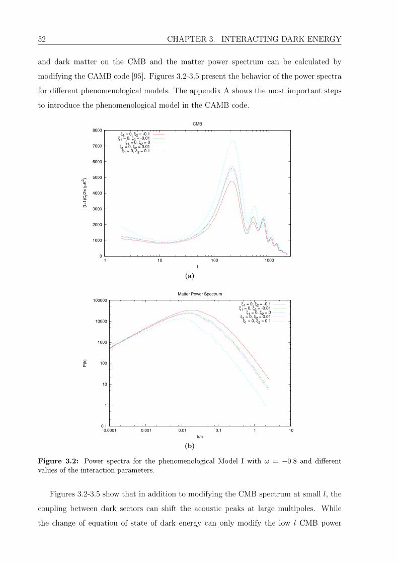
52 CHAPTER 3. INTERACTING DARK ENERGY
and dark matter on the CMB and the matter power spectrum can be calculated by
modifying the CAMB code [95]. Figures 3.2-3.5 present the behavior of the power spectra
for different phenomenological models. The appendix A shows the most important steps
to introduce the phenomenological model in the CAMB code.
0
1000
2000
3000
4000
5000
6000
7000
8000
1 10 100 1000
l(l+
1)C
l/2π (
µK
2)
l
CMB
ξ1 = 0, ξ2 = -0.1ξ1 = 0, ξ2 = -0.01
ξ1 = 0, ξ2 = 0ξ1 = 0, ξ2 = 0.01
ξ1 = 0, ξ2 = 0.1
(a)
0.1
1
10
100
1000
10000
100000
0.0001 0.001 0.01 0.1 1 10
P(k
)
k/h
Matter Power Spectrum
ξ1 = 0, ξ2 = -0.1ξ1 = 0, ξ2 = -0.01
ξ1 = 0, ξ2 = 0ξ1 = 0, ξ2 = 0.01
ξ1 = 0, ξ2 = 0.1
(b)
Figure 3.2: Power spectra for the phenomenological Model I with ω = −0.8 and differentvalues of the interaction parameters.
Figures 3.2-3.5 show that in addition to modifying the CMB spectrum at small l, the
coupling between dark sectors can shift the acoustic peaks at large multipoles. While
the change of equation of state of dark energy can only modify the low l CMB power
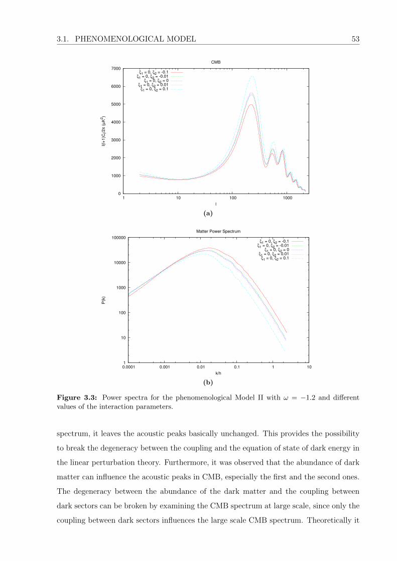
3.1. PHENOMENOLOGICAL MODEL 53
0
1000
2000
3000
4000
5000
6000
7000
1 10 100 1000
l(l+
1)C
l/2π (
µK
2)
l
CMB
ξ1 = 0, ξ2 = -0.1ξ1 = 0, ξ2 = -0.01
ξ1 = 0, ξ2 = 0ξ1 = 0, ξ2 = 0.01
ξ1 = 0, ξ2 = 0.1
(a)
1
10
100
1000
10000
100000
0.0001 0.001 0.01 0.1 1 10
P(k
)
k/h
Matter Power Spectrum
ξ1 = 0, ξ2 = -0.1ξ1 = 0, ξ2 = -0.01
ξ1 = 0, ξ2 = 0ξ1 = 0, ξ2 = 0.01
ξ1 = 0, ξ2 = 0.1
(b)
Figure 3.3: Power spectra for the phenomenological Model II with ω = −1.2 and differentvalues of the interaction parameters.
spectrum, it leaves the acoustic peaks basically unchanged. This provides the possibility
to break the degeneracy between the coupling and the equation of state of dark energy in
the linear perturbation theory. Furthermore, it was observed that the abundance of dark
matter can influence the acoustic peaks in CMB, especially the first and the second ones.
The degeneracy between the abundance of the dark matter and the coupling between
dark sectors can be broken by examining the CMB spectrum at large scale, since only the
coupling between dark sectors influences the large scale CMB spectrum. Theoretically it

54 CHAPTER 3. INTERACTING DARK ENERGY
0
2000
4000
6000
8000
10000
12000
1 10 100 1000
l(l+
1)C
l/2π (
µK
2)
l
CMB
ξ1 = 0, ξ2 = 0ξ1 = 0.01, ξ2 = 0
ξ1 = 0.1, ξ2 = 0
(a)
0.01
0.1
1
10
100
1000
10000
100000
0.0001 0.001 0.01 0.1 1 10
P(k
)
k/h
Matter Power Spectrum
ξ1 = 0, ξ2 = 0ξ1 = 0.01, ξ2 = 0
ξ1 = 0.1, ξ2 = 0
(b)
Figure 3.4: Power spectra for the phenomenological Model III with ω = −1.2 and differentvalues of the interaction parameters.
was observed that there are possible ways to break the degeneracy between the interaction,
dark energy equation of state and the dark matter abundance in the perturbation theory
[44]. This can help to get tight constraint on the interaction between dark energy and
dark matter.

3.2. LAGRANGIAN MODEL 55
0
2000
4000
6000
8000
10000
12000
1 10 100 1000
l(l+
1)C
l/2π (
µK
2)
l
CMB
ξ1 = 0, ξ2 = 0ξ1 = 0.01, ξ2 = 0.01
ξ1 = 0.1, ξ2 = 0.1
(a)
0.01
0.1
1
10
100
1000
10000
100000
0.0001 0.001 0.01 0.1 1 10
P(k
)
k/h
Matter Power Spectrum
ξ1 = 0, ξ2 = 0ξ1 = 0.01, ξ2 = 0.01
ξ1 = 0.1, ξ2 = 0.1
(b)
Figure 3.5: Power spectra for the phenomenological Model IV with ω = −1.2 and differentvalues of the interaction parameters.
3.2 Lagrangian Model
It would be desirable to construct a more fundamental model for dark matter, dark energy
and a possible interaction between them. As we know, the fundamental particles and the
corresponding interactions in the standard model are described by quantum field theories.
In the same way, we would like to account with dark matter and dark energy in the context
of a quantum field theory. However, as we already saw, the standard model of particle
56 CHAPTER 3. INTERACTING DARK ENERGY
physics have no explanation for the dark sector. Thus, in this section, we postulate a
model for dark matter interacting with dark energy.
3.2.1 The Tetrad Formalism
We are interested in the behavior of the fields on cosmological scale which means we need
a field theory on a curved spacetime. We could be tempted to follow the general approach
to transform the special-relativistic equations into general-relativistic equations chang-
ing the tensors Tα···β··· , the derivatives ∂/∂α and the metric ηαβ to tensors T µ···ν··· , covariant
derivatives ∇µ and metric gµν in the general coordinate frame. However, there are no
representations of the general-coordinate transformation group which behave like spinors
under the Lorentz subgroup. Thus, to deal with a fermionic field in the context of general
relativity we need the tetrad formalism [57].
Using the Principle of Equivalence, we can establish, at every point X, a set of coordi-
nates ξαX that are locally inertial. In the locally inertial frame, the metric is the Minkowski
one, ηαβ. Thus, we can obtain the metric in a general noninertial coordinate system xµ
as 3
gµν(x) = eαµ(x)eβν (x)ηαβ, (3.24)
where
eαµ(X) ≡(∂ξαX(x)
∂xµ
)x=X
. (3.25)
Fixing the locally inertial coordinates ξαX at each physical point X, the partial derivatives
eαµ change under a general coordinate transformation xµ → x′µ as
eαµ → e′αµ =
∂xν
∂x′µeαν . (3.26)
Thus, we can identify eαµ with four covariant vector fields, and this set of four vectors
is called a tetrad, or vierbien. On the other hand, the tetrad behaves like a Lorentz
contravariant vector under a Lorentz transformation Λαβ(x) of the locally inertial frame:
eαµ → e′αµ = Λα
β(x)eβµ. (3.27)
3We use Greek letters from the beginning of the alphabet (α, β, · · · ) to describe coordinates in thelocally inertial frame, while we use Greek letters from the end of the alphabet (µ, ν, · · · ) to describe ageneral coordinate system.

3.2. LAGRANGIAN MODEL 57
Given a contravariant vector Aµ, we can contract it with the tetrad eαµ such that the
resulting object Aα = eαµAµ transforms as a set of four scalars under a general coordinate
transformation, while it transforms as a Lorentz contravariant vector under a Lorentz
transformation of the locally inertial coordinate system. In general, a tensor n times
contravariant and m times covariant T µ1···µnν1···νm , having its contravariant indices contracted
with eαµ and its covariant indices contracted with the inverse tetrad eνβ = ηαβgµνeαµ, will
transform as a set of n × m scalars under a general transformation, and as a Lorentz
tensor n times contravariant and m times covariant under a Lorentz transformation of
the local frame.
A matter action physically acceptable must be both a scalar under a general coordinate
transformation and under a locally inertial Lorentz transformation. If an action could be
obtained solely from fields, this condition would be automatically achieved. However,
any physically sensible action must also involve derivatives of the fields. Let us consider
a field Ψ (where Ψ can be a field of multiple components), which transforms under a
Lorentz transformation as Ψ′(x) = D(Λ(x))Ψ(x), where D(Λ) is a matrix representation
of the Lorentz group. What we need is to define a covariant derivative that for a local
Lorentz transformation behaves as ∇′βΨ′ = ΛαβD(Λ)∇αΨ. We can verify that the following
covariant derivative obeys such a condition [57]:
∇α ≡ eµα(∂µ + Γµ) = eµα
[∂µ +
1
2σβδeνβ(x) (∇µeδν(x))
], (3.28)
where ∇µeδν(x) ≡ ∂µeδν(x)− Γλµνeδλ(x) and σβδ are the generators of the Lorentz group.
For example, scalars have σβδ = 0 and ∇α = ∂α, while spinors have σβδ = 14[γβ, γδ], where
γβ are Dirac matrices.
Finally we have a prescription to generalize a field theory to curved spacetimes: given a
Lagrangian which is a function of the fields and their derivatives, we contract all vectors,
tensors, etc., with the tetrad (e.g. Aα → eαµAµ) and substitute the derivatives ∂α for
covariant derivatives ∇α. Using this prescription, the action will be a scalar under a
general coordinate transformation and under a local Lorentz transformation.
The energy-momentum tensor can be defined as [57]
Tµν(x) ≡ − eαµ(x)
det[e(x)]
δSMδeνα(x)
, (3.29)
58 CHAPTER 3. INTERACTING DARK ENERGY
where SM denotes the action of the matter fields and det[e(x)] =√−g, where g is the
determinant of the metric tensor. It is possible to show that the energy-momentum tensor
defined in this way is symmetric and obeys the conservation equation ∇µTµν = 0. Using
the definition above, we can obtain the energy-momentum tensor for fields with spin in a
curved spacetime.
3.2.2 Yukawa-Type Interaction
Let us consider now a model of interaction between dark energy and dark matter from
a Lagrangian density. In this model, the dark energy will be described by a scalar field
φ and the dark matter will be described by a massive fermionic field of spin-12
Ψ 4. We
will suppose that the interaction between them is realized by an Yukawa type interaction,
which is the only interaction between a scalar field and a fermionic field of spin-12
that is
renormalizable. Thus, the action for this model will be given by
SM =
∫d4x√−g−1
2∂µφ∂
µφ− V (φ) +i
2
[Ψγµ∇µΨ− (∇µΨ)γµΨ
]− (M − βφ)ΨΨ
,
(3.30)
where β is a dimensionless interaction constant and V (φ) is the scalar potential. γµ are
matrices in the curved spacetime identified with the Dirac matrices γα multiplied by the
tetrad as γµ ≡ eµαγα and they obey the anti-comutation relation
γµ, γν = −2gµν(x). (3.31)
Varying the action SM with respect to the Dirac field Ψ and the adjoint Ψ, we obtain
the equations of motion for the fermionic fields
iγµ∇µΨ− MΨ = 0 (3.32)
and
i(∇µΨ)γµ + MΨ = 0, (3.33)
where M ≡ M − βφ. Using these equations, we can show that the current defined as
4Note that φ and Ψ here are scalar and fermionic fields, respectively. Do not confuse with the metricperturbations defined in the previous chapter.

3.2. LAGRANGIAN MODEL 59
jµ(x) =√−gΨγµΨ is conserved
∂µjµ(x) = 0. (3.34)
On the other hand, varying the action with respect to the scalar field φ, we obtain its
equation of motion
∇µ∂µφ− dV
dφ= −βΨΨ, (3.35)
where ∇µ is the covariant derivative in the curved spacetime.
The energy-momentum tensor of the system can be calculated using Eq. (3.29). For
our scalar and fermionic fields described by the action (3.30), we can show that [97]
T φµν(x) = ∂µφ∂νφ− gµν(1
2gαβ∂αφ∂βφ+ V (φ)) (3.36)
and
TΨµν(x) =
i
4
[(∇µΨ)γνΨ + (∇νΨ)γµΨ− Ψγµ∇νΨ− Ψγν∇µΨ
]. (3.37)
We have split the energy-momentum tensor by defining a scalar part and a fermionic part
such that
Tµν(x) = T φµν(x) + TΨµν(x) (3.38)
and the interaction was included in the fermionic part.
On large scales, we assume that the components in the Universe can be described by a
fluid with energy-momentum tensor given by Eq. (1.7). Thus, from the energy-momentum
tensor of a perfect fluid, we find that
ρ = −T 00 and P =
1
3T ii . (3.39)
Therefore, using the energy-momentum tensor of the scalar field (3.36), we can identify
an energy density and a pressure given by
ρφ = −1
2(∂µφ∂
µφ) + V (φ) (3.40)
and
Pφ = −1
2(∂µφ∂
µφ)− V (φ). (3.41)
On the other hand, from the energy-momentum tensor of the fermionic field (3.37), we

60 CHAPTER 3. INTERACTING DARK ENERGY
have
ρΨ = MΨΨ +i
2
[(∇iΨ
)γiΨ− Ψγi∇iΨ
](3.42)
and
PΨ =i
6
[(∇iΨ
)γiΨ− Ψγi∇iΨ
]. (3.43)
We observe that in the relativistic limit M = 0, we recover the equation of state for an
ideal relativistic gas, PΨ = ρΨ/3.
Let us assume that the Universe obeys the FLRW metric and the fields are homoge-
neous such that ∂iφ = 0, ∂iΨ = ∂iΨ = 0 and(∇iΨ
)γiΨ− Ψγi∇iΨ = 0. Thus, the energy
density and pressure of the fields result
ρφ =1
2φ2 + V (φ) (3.44)
Pφ =1
2φ2 − V (φ) (3.45)
ρΨ = MΨΨ (3.46)
PΨ = 0. (3.47)
From the above equations we observe that the scalar field possesses an equation of state
given by
ωφ ≡Pφρφ
=φ2 − 2V
φ2 + 2V. (3.48)
Besides the relations above, in a FLRW universe, the equation of motion for the scalar
field (3.35) yields
φ+ 3Hφ+dV
dφ= βΨΨ (3.49)
and the current conservation of the fermionic field (3.34) gives
d(a3Ψ†Ψ)
dt= 0. (3.50)
Deriving equations (3.44) and (3.46) with respect to the cosmic time and using the
equations of motion for the scalar and fermionic fields, we obtain the energy balance
equations
ρφ + 3Hρφ(1 + ωφ) = βφΨΨ = Q (3.51)

3.2. LAGRANGIAN MODEL 61
and
ρΨ + 3HρΨ = −βφΨΨ = −Q. (3.52)
From Eq. (3.46), we see that the interaction Q ≡ βφΨΨ can be rewritten as
Q ≡ βφΨΨ = −∂ ln M
∂φρΨφ =
β
M − βφρΨφ. (3.53)
Thus, we observe that the fermionic field can be completely described by a fluid, since the
energy balance equations depend on the fermionic field only through the energy density
ρΨ and a constant mass M . On the other hand, the scalar field cannot be completely
described by the energy balance equations because the equation of state ωφ and the
interaction termQ depend on the scalar field and its derivative. Therefore, the background
equations describing the evolution of the fermionic and scalar fields are
ρΨ + 3HρΨ = − β
M − βφρΨφ (3.54)
and
φ+ 3Hφ+dV
dφ=
β
M − βφρΨ. (3.55)
Let us introduce now linear perturbations in our model. To facilitate the study of
linear perturbations, we assume that the fermionic field can be completely described by
the fluid equations even in the perturbed level. The interaction between the dark energy
and dark matter can be generalized into a covariant form as
Qµ =∂ ln M
∂φρΨ∂
µφ. (3.56)
Thus, the balance equations can be generalized to
∇µTµνφ = Qν =
β
M − βφρΨ∇νφ (3.57)
and
∇µTµνΨ = −Qν = − β
M − βφρΨ∇νφ, (3.58)
where T µνΨ assumes the form of a perfect fluid as in Eq. (3.6). The scalar field can be
decomposed into a homogeneous part and a perturbed part, φ(t) + ϕ(t, ~x). Thus, using
62 CHAPTER 3. INTERACTING DARK ENERGY
the metric (2.6) in the synchronous gauge, the balance equations (3.57) and (3.58) yield
the perturbed equations
ϕ′′ + 2Hϕ′ + k2ϕ+ a2d2V
dφ2ϕ+
h′φ′
2= −a2 β2
(M − βφ)2ϕρΨ + a2 β
M − βφρΨδΨ, (3.59)
δ′Ψ = −h′
2− kvΨ −
β
M − βφϕ′ +
β2
(M − βφ)2φ′ϕ, (3.60)
v′Ψ = −HvΨ +β
M − βφvΨφ
′ − k β
M − βφϕ, (3.61)
in the Fourier space and conformal time.
To complete the discussion about the linear perturbations we need the initial condi-
tions of the perturbed quantities. We assume that the dark matter and the dark energy
satisfy adiabatic initial conditions
δρφρφ + Pφ
=δρΨ
ρΨ + PΨ
, (3.62)
where using equations (3.44) and (3.45) in the conformal time, we have
δρφ =φ′ϕ′
a2+dV
dφϕ and δPφ =
φ′ϕ′
a2− dV
dφϕ. (3.63)
Thus, the adiabatic initial condition (3.62) can be rewritten as
φ′ϕ′ + a2 dVdφϕ
φ′2= δΨ. (3.64)
As the scalar field obeys a second-order differential equation, we need two initial condi-
tions. The second initial condition can be obtained considering that the intrinsic entropy
is nullδρφρφ− δPφ
Pφ= 0, (3.65)
which impliesφ′ϕ′ + a2 dV
dφϕ
φ′2
2+ a2V
=φ′ϕ′ − a2 dV
dφϕ
φ′2
2− a2V
. (3.66)
Finally, solving equations (3.64) and (3.66) for ϕ and ϕ′, we obtain the perturbed initial
conditions for the scalar field
ϕ =2δΨφ
′2V
(φ′2 + 2a2V )dVdφ
(3.67)

3.2. LAGRANGIAN MODEL 63
and
ϕ′ =δΨφ
′3
φ′2 + 2a2V. (3.68)
We modified the CAMB code to include the Lagrangian model above. We considered
that the scalar potential is given by
V (φ) = Ae−λφ/Mpl , (3.69)
where A is a normalization constant, λ is a dimensionless parameter and Mpl is the reduced
Planck mass. We set A to the value of the cosmological constant energy density A = ρΛ.
Thus, λ 6= 0 and β 6= 0 is a measurement of how our model differ from the cosmological
constant model. We also see from Eq. (3.53) that the interaction β and the fermion mass
M are degenerate, we can only know the ratio r ≡ βMMpl. Therefore, we use r instead
of β as our interaction parameter. This has the advantage of decreasing one degree of
freedom in the analysis, at the cost that we are unable to know the individual values of
β or M .
The appendix B shows the most import steps to introduce the Lagrangian model in
the CAMB code. Below we present some graphs for the CMB and matter power spectrum
obtained from the Lagrangian model for different values of the parameters. Figure 3.6
shows that the scalar potential parameter λ has a small effect on the CMB and matter
power spectrum, affecting mainly the low-l CMB power spectrum. On the other hand, as
observed in the phenomenological case, we see from Fig. 3.7 that in addition to modifying
the CMB spectrum at low l, the coupling between dark sectors can shift the acoustic peaks
at large multipoles. However, comparing with the phenomenological models, the Yukawa
interaction has a more dramatic effect on low multipoles and less effect on the acoustic
peaks. We also observe that the power spectra present an almost symmetric behavior
around the zero value for the interaction. However, such a symmetry is broken when we
look at background quantities, e.g. the age of the Universe.

64 CHAPTER 3. INTERACTING DARK ENERGY
0
1000
2000
3000
4000
5000
6000
1 10 100 1000
l(l+
1)C
l/2π (
µK
2)
l
CMB
λ = 0.1λ = 0.5λ = 1.0λ = 1.5
(a)
1
10
100
1000
10000
100000
0.0001 0.001 0.01 0.1 1 10
P(k
)
k/h
Matter Power Spectrum
λ = 0.1λ = 0.5λ = 1.0λ = 1.5
(b)
Figure 3.6: Power spectra for the Lagrangian model with r = βMMpl = 0 and different values
for the scalar potential parameter.
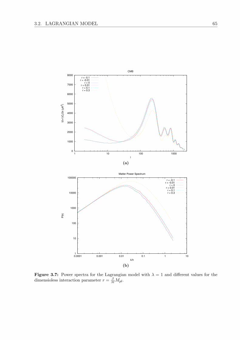
3.2. LAGRANGIAN MODEL 65
0
1000
2000
3000
4000
5000
6000
7000
8000
1 10 100 1000
l(l+
1)C
l/2π (
µK
2)
l
CMB
r = -0.1r = -0.01
r = 0r = 0.01
r = 0.1r = 0.3
(a)
1
10
100
1000
10000
100000
0.0001 0.001 0.01 0.1 1 10
P(k
)
k/h
Matter Power Spectrum
r = -0.1r = -0.01
r = 0r = 0.01
r = 0.1r = 0.3
(b)
Figure 3.7: Power spectra for the Lagrangian model with λ = 1 and different values for thedimensioless interaction parameter r = β
MMpl.
Chapter 4
Analysis
In the previous chapter we presented some models of interacting dark energy. We showed
some aspects of their behavior, especially on the power spectra. We now wish to test such
models with current observational data in order to constrain the cosmological parameters.
The results of this chapter are matter of publication in [98–100].
4.1 Methods for Data Analysis
Let us suppose we want to estimate a random physical quantity x with a probability density
function (PDF) f(x|θ) that depends on an unknown parameter θ. Naturally, we cannot
know the exact value of x, since there are several uncertainties in the measurement, which
we denote as σ. Then, the probability of obtaining x in the interval ∆x around x is
P =
∫ x2
x1
f(x|θ)dx. (4.1)
Such a probability is called a conditional probability of having the data x given the theo-
retical parameter θ. If the interval of integration above is small, we can approximate the
probability as P ≈ f(x|θ)∆x.
The law of joint probability tells us that for several measurements xi, i = 1, ..., N , the
probability of having x1 in the interval ∆x1 around x1, x2 in the interval ∆x2 around x2
and so forth is
P (xi|θ) ≈ (∆x)NN∏i=1
f(xi|θ) ≡ (∆x)NL(xi|θ). (4.2)
This procedure is correct given the fact that the measurements are mutually independent
66
4.1. METHODS FOR DATA ANALYSIS 67
and considering equally spaced small intervals ∆xi. In the above expression we defined the
likelihood function, L(xi|θ) ≡∏N
i=1 f(xi|θ). Except for a constant value, the likelihood
function gives us the probability of having the outcomes xi given the parameter θ. In
general, the data can be correlated and depend on several parameters θj. For correlated
data, L(xi|θj) will not be the simple product of the PDFs, but its statistical interpretation
remains the same.
For every set of parameters θj, the likelihood function L(xi|θj) will assume a different
value. It is logic to define the best θjs as the parameters that maximize the likelihood.
Thus, the maximum likelihood method of parameter estimation consists in finding the
parameters that maximize the likelihood solving the system
∂L(xi|θj)∂θj
= 0, j = 1, · · · ,m. (4.3)
The solutions of these equations, θjs, are functions of the random data xis, therefore they
are random too. In the frequentist approach, one tries to find the distribution of the θjs
given the distribution of the data xis; if this is possible, one can associate probabilities to
intervals of θjs, for instance determine the interval of θj that has 95% probability that a set
of data were obtained from the theoretical distribution. However, it is often too difficult to
derive the θj’s distributions analytically and very demanding to derive them numerically
using simulated datasets. Moreover, this approach does not take into account our previous
knowledge about the theoretical parameters, e.g. the results of preceding experiments.
These issues can be worked more appropriately using the Bayesian approach.
In the Bayesian approach, instead of looking for the probability of having the data
given the model, L(xi|θj), we look for the probability of the model given the data, P (θj|xi).
This is possible thanks to the Bayes’s theorem,
P (B|A, I) =P (A|B, I)P (B|I)
P (A|I), (4.4)
which relates the conditional probability of having an event B given the event A occurred,
P (B|A, I), with the conditional probability P (A|B, I) of A given B and the probabilities
P (B|I) and P (A|I) of the events B and A, respectively. The letter “I” denotes that these
probabilities depend on some information I we assume to be true.
In our case we have the data A ≡ xi and the parameters B ≡ θj for some theoretical

68 CHAPTER 4. ANALYSIS
model I ≡M , thus
p(θj|xi,M) =L(xi|θj)p(θj|M)
p(xi|M). (4.5)
The function p(θj|xi,M) is the posterior probability distribution, p(xi|M) is the PDF
of the data xi, sometimes called evidence, and p(θj|M) is the prior probability for the
parameters θj, it represents our previous knowledge for the parameters before we make
the experiment. Therefore, the posterior contains the information we are looking for: the
probability of having the parameters θj given the data xi and some previous knowledge
about the parameters.
The posterior is a probability distribution and consequently it must be normalized to
unity ∫p(θj|xi,M)dmθj =
∫L(xi|θj)p(θj|M)dmθj
p(xi|M)= 1, (4.6)
which implies ∫L(xi|θj)p(θj|M)dmθj = p(xi|M). (4.7)
Thus, we can think the evidence as a normalization factor. On the other hand, the prior
is often unknown. Usually, if we know nothing about the parameters we want to estimate,
we choose a uniform prior in some interval and zero outside it. However, if we have some
estimate of the parameters from previous experiments, we can adopt a Gaussian centered
at the estimated value as our prior. In general, the choice of priors affect the posterior
distribution, but if we have enough data they will dominate the posterior.
Given the posterior p(θj|xi,M) we can find the maximum likelihood estimators θj as
∂p(θj|xi,M)
∂θj= 0 j = 1, · · · ,m. (4.8)
We can also derive the regions of confidence for the parameters, which are defined as
regions R(α) such that ∫R(α)
p(θj|xi,M)dmθ = α, (4.9)
where the posterior must be normalized, which means 0 < α < 1. To find these regions,
the limits of integration must be the lowest ones such that the integral is valid. Typical
choices of α are α = 0.683, 0.954, 0.997 which denote the 1σ, 2σ and 3σ confidence levels.
Frequently, we are interested in a subset of the parameter space and we consider the
others as “nuisance”, thus we integrate (marginalize) over the uninterested parameters.
4.2. DATA 69
In general, the distribution function depends on the characteristics of the quantity it
describes and its uncertainties. In cosmology we usually assume a Gaussian distribution
for the data even when each data was not extracted from a Gaussian distribution. This is
possible thanks to the central limit theorem [101, 102], which establishes that for a set of
N variables with some distribution each one with a finite variance, in the limit N →∞,
the average distribution tends to a Gaussian one. Thus, if the data have a Gaussian
distribution and are independent of each other, then
L(xi|θj) =N∏i=1
1√2πσi
exp
[−1
2
(xi − xi(θj)
σi
)2]
=
(N∏i=1
1√2πσi
)exp
[−1
2
N∑i=1
(xi − xi(θj)
σi
)2]. (4.10)
Therefore, maximizing the posterior distribution (4.5) is equivalent to minimizing the
above exponent
χ2 ≡N∑i=1
(xi − xi(θj)
σi
)2
. (4.11)
If the data are correlated, the above likelihood must be generalized as
L(xi|θj) ∝1√
detCexp
(−1
2XTC−1X
), (4.12)
where X is the data vector and C is the covariance matrix.
4.2 Data
To constrain the cosmological parameters in our interacting models, we use several data
sets, the measurements of CMB anisotropies, BAO, SNIa, the direct measurement of the
Hubble constant H0 and Lookback Time. Below we describe the likelihood for these
measurements.
4.2.1 CMB Measurements
The Planck data set we use is a combination of the low-l TT likelihood, which includes
measurements for l = 2 − 49, combined with the high-l TT likelihood, which includes
measurements from l = 50 up to a maximum multipole number of lmax = 2500 [47–49].
70 CHAPTER 4. ANALYSIS
Together with the Planck data, we include the polarization measurements from the nine
year Wilkinson Microwave Anisotropy Probe (WMAP) [103], the low-l (l < 32) TE, EE,
BB likelihoods.
The CMB power spectrum likelihood for low-l multipoles can be written as
L(Cl) = p(m|Cl) =1
2πn/2|M|1/2exp
(−1
2mtM−1m
), (4.13)
where n is the number of observed pixels, M(Cl) = C(Cl) + N is the data covariance
matrix, which is split into the CMB, C, and noise, N, covariance matrices, and m = s + n
is the observed map. Actually, the estimated Cl distribution is not well approximate by
a Gaussian at low l (l < 50), because of the limited degrees of freedom per l. However,
if foregrounds and instrumental systematics are negligible, then the CMB signal s and
instrumental noise n are nearly Gaussian and the above likelihood is valid.
In the general case, the data vector m includes both temperature and linear polariza-
tion. For the temperature, the signal covariance matrix gives
〈Ti1Ti2〉 =lmax∑l=2
2l + 1
4πCthl b
2lW
2l Pl(θi1i2) + Ni1i2 , (4.14)
where Pl are Legendre polynomials calculated at angle θi1i2 between the centers of pixels
i1 and i2, bl is the effect of instrumental beam and Wl is the window function. For
polarization correlations, we obtain similar expressions.
4.2.2 BAO Measurements
In addition to the CMB data sets, we also consider measurements of Baryon Acoustic
Oscillations (BAO) in the matter power spectrum. We combine the results from three
redshift surveys: the 6dF Galaxy Survey measurement at redshift z = 0.106 [50], the
SDSS DR7 BAO measurement at redshift z = 0.35 as analysed by Padmanabhan et al.
[51] and the BOSS DR9 measurement at z = 0.57 [52].
These redshift surveys measure the distance ratio
dz =rs(zdrag)
DV (z), (4.15)
where rs(zdrag) is the comoving sound horizon at the baryon drag epoch, the epoch when
4.2. DATA 71
baryons became dynamically decoupled from photons, and DV (z) combines the angular
diameter distance dA(z) and the Hubble parameter H(z), in a way appropriate for the
analysis of spherically-averaged two-point statistics,
DV (z) =
[(1 + z)2d2
A(z)cz
H(z)
]1/3
. (4.16)
The comparison with BAO measurements is made using χ2 statistics
χ2BAO = (x− xobs)TC−1
BAO(x− xobs), (4.17)
where x is our theoretical predictions and xobs denotes the data vector. The data vector
is composed by the measurements of the three data sets above: For the 6dF DV (0.106) =
(457± 27)Mpc, for the DR7 DV (0.35)/rs = 8.88± 0.17 and for the DR9 DV (0.57)/rs =
13.67± 0.22.
4.2.3 SNIa Measurements
We use the SNIa data from the Supernova Cosmology Project (SCP) Union 2.1 compi-
lation [53], which has 580 samples. The Union 2.1 uses SALT2 [104] to fit supernova
lightcurves. The SALT2 model fits three parameters to each supernova: an overall nor-
malization, x0, to the time dependent spectral energy distribution of a SNIa, the deviation
from the average lightcurve shape x1 and the deviation from the mean SNIa B - V color
c. Combining these parameters, the distance modulus is given by
µB = mmaxB + α · x1 − β · c+ δ · P (mtrue
? < mthreshold? )−MB, (4.18)
where mmaxB is the integrated B-band flux at maximum light, P (mtrue
? < mthreshold? ) gives
the correlation of SNIa luminosity to the mass of the host galaxy and MB is the absolute
B-band magnitude. The nuisance parameters α, β, δ and MB are fitted simultaneously
with cosmological parameters.
The best-fit cosmology is determined by minimizing the χ2,
χ2SN =
580∑i=1
[µB(α, β, δ,MB)− µ(z,Ωm,Ωd, w)]2
σ2. (4.19)

72 CHAPTER 4. ANALYSIS
To test our interacting dark energy models we use the CosmoMC [105, 106] module
associated with the Union 2.1 sample. In this module the nuisance parameters are hold
fixed with values α = 0.1218, β = 2.4657 and δ = −0.03634.
4.2.4 H0 Measurements
From observations of Cepheid variables and low-redshift Type Ia surpernovae, the Hubble
Space Telescope (HST) determined the Hubble constant with 3.3% uncertainty including
systematic errors [54]
H0 = 73.8± 2.4kms−1Mpc−1. (4.20)
We use this measurement of the Hubble constant as an additional data.
4.2.5 Lookback Time Measurements
The background observables treated so far, the measurements of H0 and SNIa, are firmed
on distance measurements. To pin down the cosmological parameters we will consider
another indicator, the lookback time, which is based on ages instead of distances. The
lookback time tL(z) is the difference between the present age of the Universe, t0, and its
age at redshift z, t(z),
tL(z) = t0 − t(z) =
∫ ∞0
dz′
(1 + z′)H(z′)−∫ ∞z
dz′
(1 + z′)H(z′)=
∫ z
0
dz′
(1 + z′)H(z′). (4.21)
For an object at redshift zi, we can calculate its age from the difference between the age
of the Universe at redshift zi and the age of the Universe when the object was formed at
redshift zF ,
t(zi) =
∫ ∞zi
dz′
(1 + z′)H(z′)−∫ ∞zF
dz′
(1 + z′)H(z′)=
∫ zF
zi
dz′
(1 + z′)H(z′)= tL(zF )− tL(zi),
(4.22)
where we used the lookback time definition (4.21). Thus, the above equation tells us that
the observed lookback time tobsL (zi) to an object i at redshift zi is
tobsL (zi) = tL(zF )− t(zi) = [tobs0 − t(zi)]− [tobs0 − tL(zF )] = tobs0 − t(zi)− df, (4.23)
4.3. RESULTS 73
where df ≡ tobs0 − tL(zF ) is the delay factor which encodes our ignorance of the formation
redshift zF .
In order to constrain the cosmological parameters, we implement a CosmoMC module
to calculate the likelihood for lookback time measurements (Appendix C shows the details
of this module). We use the data of 32 passively evolving galaxies in the redshift interval
0.117 ≤ z ≤ 1.845 with an uncertainty in the age measurements of 12% at one standard
deviation [56]. Additionally, we use the ages of 6 galaxy clusters in the redshift range
0.10 ≤ z ≤ 1.27 with an uncertainty of 1Gyr at one standard deviation [55]. The likelihood
is a Gaussian with
χ2LBT =
38∑i=1
[tL(zi, ~p)− tobsL (zi, df)]2
σ2i + σ2
tobs0
+[t0(~p)− tobs0 ]2
σ2tobs0
, (4.24)
where ~p denotes the theoretical cosmological parameters. The delay factor is a nuisance
parameter that is fitted simultaneously with the cosmological parameters.
4.3 Results
4.3.1 Phenomenological Model
We would like to put constraints on the four phenomenological coupled dark energy models
listed in Table 3.1. For this purpose, we will use the recent measurements of the cosmic
microwave background anisotropies as measured by the Planck satellite mission. We
will also consider the combined constraints from the Planck data plus BAO, SNIa and
H0 measurements. In our analysis, we will choose our priors of different cosmological
parameters as listed in Table 4.1. The results were published in [98].
We will allow the equation of state of dark energy to vary. We also choose the helium
abundance Yp from a big bang nucleosynthesis (BBN) consistent scenario. Thus, the
primordial helium abundance Yp is predicted as a function of the baryon density Ωbh2
and number of extra radiation degrees of freedom ∆N . We will use interpolated results
from the PArthENoPE code [107] to set Yp, following [108]. We will take the relativistic
number of degrees of freedom Neff = 3.046, the total neutrino mass∑mν = 0.06eV and
the spectrum lensing normalization AL = 1. To compare theory with observations, we
employ the Markov chain Monte Carlo (MCMC) methodology through a modified version
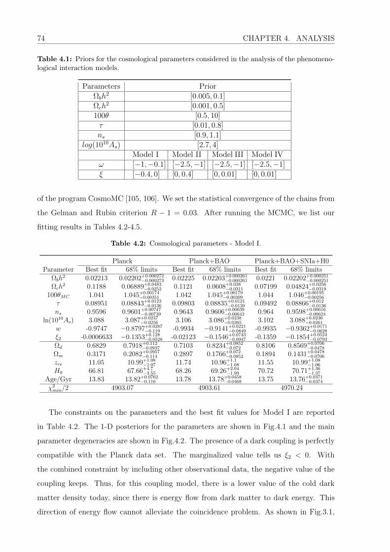
74 CHAPTER 4. ANALYSIS
Table 4.1: Priors for the cosmological parameters considered in the analysis of the phenomeno-logical interaction models.
Parameters PriorΩbh
2 [0.005, 0.1]Ωch
2 [0.001, 0.5]100θ [0.5, 10]τ [0.01, 0.8]ns [0.9, 1.1]
log(1010As) [2.7, 4]Model I Model II Model III Model IV
ω [−1,−0.1] [−2.5,−1] [−2.5,−1] [−2.5,−1]
ξ [−0.4, 0] [0, 0.4] [0, 0.01] [0, 0.01]
of the program CosmoMC [105, 106]. We set the statistical convergence of the chains from
the Gelman and Rubin criterion R − 1 = 0.03. After running the MCMC, we list our
fitting results in Tables 4.2-4.5.
Table 4.2: Cosmological parameters - Model I.
Planck Planck+BAO Planck+BAO+SNIa+H0Parameter Best fit 68% limits Best fit 68% limits Best fit 68% limits
Ωbh2 0.02213 0.02202+0.000272
−0.000273 0.02225 0.02203+0.000261−0.000261 0.0221 0.02202+0.000251
−0.000251
Ωch2 0.1188 0.06889+0.0483
−0.0252 0.1121 0.0608+0.038−0.0311 0.07199 0.04824+0.0256
−0.0319
100θMC 1.041 1.045+0.00174−0.00351 1.042 1.045+0.00179
−0.00309 1.044 1.046+0.00195−0.00256
τ 0.08951 0.08843+0.0123−0.0136 0.09803 0.08835+0.0121
−0.0139 0.09492 0.08866+0.012−0.0136
ns 0.9596 0.9601+0.00747−0.00739 0.9643 0.9606+0.00639
−0.00642 0.964 0.9598+0.00616−0.00624
ln(1010As) 3.088 3.087+0.0237−0.0256 3.106 3.086+0.0238
−0.0265 3.102 3.088+0.0236−0.0261
w -0.9747 −0.8797+0.0287−0.119 -0.9934 −0.9141+0.0221
−0.0849 -0.9935 −0.9362+0.0171−0.0628
ξ2 -0.0006633 −0.1353+0.128−0.0528 -0.02123 −0.1546+0.0743
−0.0947 -0.1359 −0.1854+0.0524−0.0793
Ωd 0.6829 0.7918+0.112−0.0937 0.7103 0.8234+0.0852
−0.072 0.8106 0.8569+0.0706−0.0478
Ωm 0.3171 0.2082+0.0957−0.114 0.2897 0.1766+0.072
−0.0852 0.1894 0.1431+0.0478−0.0706
zre 11.05 10.99+1.08−1.07 11.74 10.96+1.1
−1.08 11.55 10.99+1.08−1.06
H0 66.81 67.66+4.7−3.55 68.26 69.26+2.04
−1.99 70.72 70.71+1.36−1.37
Age/Gyr 13.83 13.82+0.0762−0.116 13.78 13.78+0.0458
−0.0468 13.75 13.76+0.0371−0.0374
χ2min/2 4903.07 4903.61 4970.24
The constraints on the parameters and the best fit values for Model I are reported
in Table 4.2. The 1-D posteriors for the parameters are shown in Fig.4.1 and the main
parameter degeneracies are shown in Fig.4.2. The presence of a dark coupling is perfectly
compatible with the Planck data set. The marginalized value tells us ξ2 < 0. With
the combined constraint by including other observational data, the negative value of the
coupling keeps. Thus, for this coupling model, there is a lower value of the cold dark
matter density today, since there is energy flow from dark matter to dark energy. This
direction of energy flow cannot alleviate the coincidence problem. As shown in Fig.3.1,
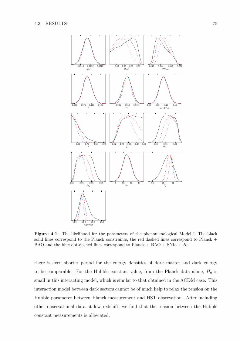
4.3. RESULTS 75
0.0216 0.0222 0.0228
Ωbh2
0.03 0.06 0.09 0.12
Ωch2
1.040 1.044 1.048 1.052100θMC
0.050 0.075 0.100 0.125τ
0.945 0.960 0.975ns
3.00 3.05 3.10 3.15
ln(1010As)
−0.90 −0.75 −0.60 −0.45w
−0.32 −0.24 −0.16 −0.08 0.00ξ2
0.60 0.75 0.90ΩΛ
0.00 0.15 0.30 0.45Ωm
8 10 12 14zre
56 64 72H0
13.6 13.8 14.0 14.2
Age/Gyr
Figure 4.1: The likelihood for the parameters of the phenomenological Model I. The blacksolid lines correspond to the Planck constraints, the red dashed lines correspond to Planck +BAO and the blue dot-dashed lines correspond to Planck + BAO + SNIa + H0.
there is even shorter period for the energy densities of dark matter and dark energy
to be comparable. For the Hubble constant value, from the Planck data alone, H0 is
small in this interacting model, which is similar to that obtained in the ΛCDM case. This
interaction model between dark sectors cannot be of much help to relax the tension on the
Hubble parameter between Planck measurement and HST observation. After including
other observational data at low redshift, we find that the tension between the Hubble
constant measurements is alleviated.

76 CHAPTER 4. ANALYSIS
−0.9 −0.8 −0.7 −0.6 −0.5w
0.025
0.050
0.075
0.100
0.125
Ωch
2
−0.30−0.24−0.18−0.12−0.06 0.00ξ2
0.025
0.050
0.075
0.100
0.125
Ωch
2−0.30−0.24−0.18−0.12−0.06 0.00
ξ2
−0.9
−0.8
−0.7
−0.6
−0.5
w
Planck Planck+BAO Planck+BAO+SN+H0
Figure 4.2: 2-D distribution for selected parameters - Model I.
Table 4.3: Cosmological parameters - Model II.
Planck Planck+BAO Planck+BAO+SNIa+H0Parameter Best fit 68% limits Best fit 68% limits Best fit 68% limits
Ωbh2 0.02201 0.02208+0.000283
−0.000277 0.02219 0.02199+0.000264−0.00026 0.02208 0.02203+0.000255
−0.000255
Ωch2 0.1308 0.1335+0.0076
−0.0118 0.132 0.1352+0.00844−0.0115 0.1432 0.1344+0.00751
−0.0118
100θMC 1.041 1.041+0.000815−0.000768 1.041 1.04+0.000747
−0.000758 1.04 1.04+0.00076−0.000757
τ 0.08672 0.08934+0.0128−0.0138 0.08154 0.08761+0.0121
−0.0137 0.08312 0.08844+0.012−0.0135
ns 0.9615 0.9599+0.00715−0.00703 0.9598 0.9581+0.00654
−0.00658 0.962 0.9586+0.00632−0.00637
ln(1010As) 3.085 3.089+0.0245−0.0267 3.078 3.088+0.0234
−0.0261 3.079 3.089+0.0232−0.0263
w -1.696 −1.516+0.312−0.305 -1.166 −1.189+0.152
−0.0721 -1.181 −1.192+0.0771−0.0715
ξ2 0.02837 0.03923+0.0121−0.0392 0.03522 0.04818+0.0164
−0.0482 0.0784 0.04562+0.0155−0.0456
Ωd 0.806 0.762+0.0799−0.0384 0.69 0.6849+0.0292
−0.0296 0.6653 0.6901+0.0253−0.0201
Ωm 0.194 0.238+0.0384−0.0799 0.31 0.3151+0.0296
−0.0292 0.3347 0.3099+0.0201−0.0253
zre 10.81 11.+1.11−1.1 10.35 10.92+1.08
−1.08 10.5 10.98+1.07−1.07
H0 88.93 82.69+9.78−11.9 70.68 70.92+2.08
−3.19 70.42 71.25+1.48−1.48
Age/Gyr 13.53 13.6+0.0942−0.148 13.74 13.76+0.0489
−0.0487 13.75 13.75+0.0373−0.0378
χ2min/2 4901.08 4903.02 4968.20
Now we present the fitting results for the coupling Model II in Table 4.3. In this model,
the interaction between the dark sectors is still proportional to the energy density of dark
energy but with equation of state of dark energy smaller than −1. From the Planck data
analysis alone, we obtain the Hubble constant value significantly larger than that in the
standard ΛCDM case, H0 = 82.69+9.78−11.9 km · s−1 ·Mpc−1. This is different from what we
observed in the fitting results of Model I, where the H0 is much smaller and consistent
with the ΛCDM case. The lower fitting range of the H0 in Model II is consistent with the
observations in the low redshift. We have explored the degeneracy between the Hubble
value and the equation of state of dark energy and found that smaller equation of state
of dark energy leads to higher value of the Hubble parameter. The coupling constant
ξ2 is found to be positive, which shows that there is an energy flow from dark energy
to dark matter. This is required to alleviate the coincidence problem, because with this

4.3. RESULTS 77
0.0216 0.0224
Ωbh2
0.120 0.135 0.150
Ωch2
1.038 1.040 1.042100θMC
0.050 0.075 0.100 0.125τ
0.945 0.960 0.975ns
3.00 3.05 3.10 3.15
ln(1010As)
−2.1 −1.8 −1.5 −1.2w
0.000 0.025 0.050 0.075 0.100ξ2
0.6 0.7 0.8ΩΛ
0.16 0.24 0.32 0.40Ωm
8 10 12 14zre
60 70 80 90 100H0
13.4 13.6 13.8
Age/Gyr
Figure 4.3: The likelihood for the parameters of the phenomenological Model II. The blacksolid lines correspond to the Planck constraints, the red dashed lines correspond to Planck +BAO and the blue dot-dashed lines correspond to Planck + BAO + SNIa + H0.
interaction there is longer period for the energy densities of dark matter and dark energy
to be comparable, which was illustrated in the Fig.3.1. Combined with other observational
data, we show that a combined analysis provides significant evidence for this coupled dark
energy with positive non-zero value of the coupling parameter, consistent Hubble constant
and equation of state of dark energy. The 1-D posteriors for the parameters are shown in
Fig.4.3 and the main parameter degeneracies are shown in Fig.4.4.
Now we turn our discussion to the coupled dark energy Model III, where the interaction
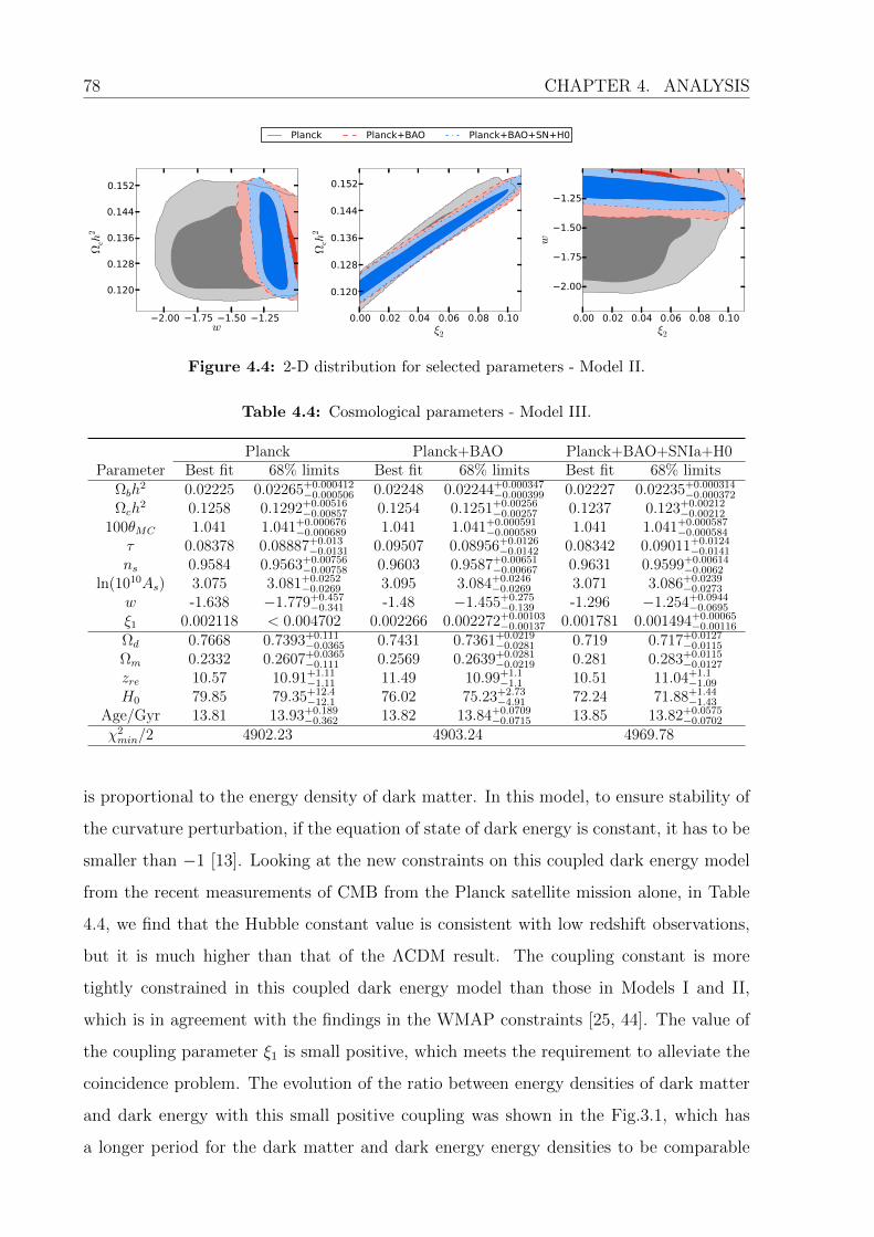
78 CHAPTER 4. ANALYSIS
−2.00 −1.75 −1.50 −1.25w
0.120
0.128
0.136
0.144
0.152
Ωch
2
0.00 0.02 0.04 0.06 0.08 0.10ξ2
0.120
0.128
0.136
0.144
0.152
Ωch
20.00 0.02 0.04 0.06 0.08 0.10
ξ2
−2.00
−1.75
−1.50
−1.25
w
Planck Planck+BAO Planck+BAO+SN+H0
Figure 4.4: 2-D distribution for selected parameters - Model II.
Table 4.4: Cosmological parameters - Model III.
Planck Planck+BAO Planck+BAO+SNIa+H0Parameter Best fit 68% limits Best fit 68% limits Best fit 68% limits
Ωbh2 0.02225 0.02265+0.000412
−0.000506 0.02248 0.02244+0.000347−0.000399 0.02227 0.02235+0.000314
−0.000372
Ωch2 0.1258 0.1292+0.00516
−0.00857 0.1254 0.1251+0.00256−0.00257 0.1237 0.123+0.00212
−0.00212
100θMC 1.041 1.041+0.000676−0.000689 1.041 1.041+0.000591
−0.000589 1.041 1.041+0.000587−0.000584
τ 0.08378 0.08887+0.013−0.0131 0.09507 0.08956+0.0126
−0.0142 0.08342 0.09011+0.0124−0.0141
ns 0.9584 0.9563+0.00756−0.00758 0.9603 0.9587+0.00651
−0.00667 0.9631 0.9599+0.00614−0.0062
ln(1010As) 3.075 3.081+0.0252−0.0269 3.095 3.084+0.0246
−0.0269 3.071 3.086+0.0239−0.0273
w -1.638 −1.779+0.457−0.341 -1.48 −1.455+0.275
−0.139 -1.296 −1.254+0.0944−0.0695
ξ1 0.002118 < 0.004702 0.002266 0.002272+0.00103−0.00137 0.001781 0.001494+0.00065
−0.00116
Ωd 0.7668 0.7393+0.111−0.0365 0.7431 0.7361+0.0219
−0.0281 0.719 0.717+0.0127−0.0115
Ωm 0.2332 0.2607+0.0365−0.111 0.2569 0.2639+0.0281
−0.0219 0.281 0.283+0.0115−0.0127
zre 10.57 10.91+1.11−1.11 11.49 10.99+1.1
−1.1 10.51 11.04+1.1−1.09
H0 79.85 79.35+12.4−12.1 76.02 75.23+2.73
−4.91 72.24 71.88+1.44−1.43
Age/Gyr 13.81 13.93+0.189−0.362 13.82 13.84+0.0709
−0.0715 13.85 13.82+0.0575−0.0702
χ2min/2 4902.23 4903.24 4969.78
is proportional to the energy density of dark matter. In this model, to ensure stability of
the curvature perturbation, if the equation of state of dark energy is constant, it has to be
smaller than −1 [13]. Looking at the new constraints on this coupled dark energy model
from the recent measurements of CMB from the Planck satellite mission alone, in Table
4.4, we find that the Hubble constant value is consistent with low redshift observations,
but it is much higher than that of the ΛCDM result. The coupling constant is more
tightly constrained in this coupled dark energy model than those in Models I and II,
which is in agreement with the findings in the WMAP constraints [25, 44]. The value of
the coupling parameter ξ1 is small positive, which meets the requirement to alleviate the
coincidence problem. The evolution of the ratio between energy densities of dark matter
and dark energy with this small positive coupling was shown in the Fig.3.1, which has
a longer period for the dark matter and dark energy energy densities to be comparable

4.3. RESULTS 79
0.022 0.023 0.024
Ωbh2
0.12 0.13 0.14 0.15
Ωch2
1.040 1.042100θMC
0.050 0.075 0.100 0.125τ
0.930 0.945 0.960 0.975ns
3.00 3.05 3.10 3.15
ln(1010As)
−2.4 −2.0 −1.6 −1.2w
0.000 0.002 0.004 0.006 0.008 0.010ξ1
0.2 0.4 0.6 0.8ΩΛ
0.2 0.4 0.6 0.8Ωm
8 10 12 14zre
45 60 75 90H0
13.6 14.0 14.4 14.8
Age/Gyr
Figure 4.5: The likelihood for the parameters of the phenomenological Model III. The blacksolid lines correspond to the Planck constraints, the red dashed lines correspond to Planck +BAO and the blue dot-dashed lines correspond to Planck + BAO + SNIa + H0.
when ξ is positive and has the attractor solution with the ratio between dark energy and
dark matter energy densities % ∼ constant in the past. We also consider the combined
constraints from the Planck data plus other measurements. The results are listed in Table
4.4, which shows stronger evidence for this coupled dark energy model with small positive
coupling. We plot the 1-D posteriors for the parameters in Fig.4.5 and show the main
parameter degeneracies in Fig.4.6.
Finally, we present the fitting results for the coupled dark energy Model IV, where
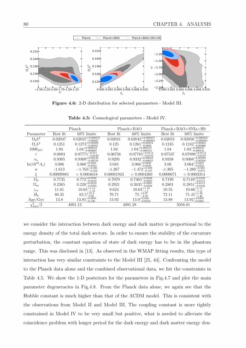
80 CHAPTER 4. ANALYSIS
−2.50−2.25−2.00−1.75−1.50−1.25w
0.120
0.128
0.136
0.144
0.152
Ωch
2
0.000 0.002 0.004 0.006 0.008 0.010ξ1
0.120
0.128
0.136
0.144
0.152
Ωch
20.000 0.002 0.004 0.006 0.008 0.010
ξ1
−2.50
−2.25
−2.00
−1.75
−1.50
−1.25
w
Planck Planck+BAO Planck+BAO+SN+H0
Figure 4.6: 2-D distribution for selected parameters - Model III.
Table 4.5: Cosmological parameters - Model IV.
Planck Planck+BAO Planck+BAO+SNIa+H0Parameter Best fit 68% limits Best fit 68% limits Best fit 68% limits
Ωbh2 0.02047 0.02037+0.000275
−0.00027 0.02041 0.02042+0.000257−0.000263 0.02053 0.02056+0.000253
−0.000265
Ωch2 0.1251 0.1273+0.00309
−0.00321 0.125 0.1261+0.00254−0.0025 0.1245 0.1242+0.00204
−0.00208
100θMC 1.04 1.04+0.000618−0.000607 1.04 1.04+0.000574
−0.000572 1.04 1.04+0.000537−0.000541
τ 0.0883 0.07771+0.011−0.0129 0.06756 0.07785+0.0112
−0.0124 0.07537 0.07899+0.0112−0.0127
ns 0.9305 0.9309+0.00746−0.00743 0.9295 0.9332+0.00643
−0.00655 0.9338 0.9368+0.00592−0.00594
ln(1010As) 3.086 3.068+0.0221−0.0253 3.045 3.066+0.0228
−0.0248 3.06 3.064+0.0227−0.0233
w -1.613 −1.763+0.385−0.432 -1.267 −1.472+0.229
−0.147 -1.305 −1.286+0.082−0.074
ξ 0.00009881 < 0.0004618 0.00001943 < 0.0004260 0.0000671 < 0.0003314Ωd 0.7735 0.772+0.0793
−0.0319 0.7079 0.7365+0.0238−0.0267 0.7199 0.7149+0.0126
−0.0115
Ωm 0.2265 0.228+0.0319−0.0793 0.2921 0.2635+0.0267
−0.0238 0.2801 0.2851+0.0115−0.0126
zre 11.61 10.65+1.14−1.12 9.624 10.63+1.14
−1.1 10.35 10.66+1.11−1.11
H0 80.35 82.5+12.4−9.95 70.71 75.+3.07
−4.59 72.11 71.45+1.48−1.46
Age/Gyr 13.8 13.85+0.0891−0.136 13.92 13.9+0.046
−0.0532 13.89 13.92+0.0385−0.0391
χ2min/2 4991.13 4991.28 5058.81
we consider the interaction between dark energy and dark matter is proportional to the
energy density of the total dark sectors. In order to ensure the stability of the curvature
perturbation, the constant equation of state of dark energy has to be in the phantom
range. This was disclosed in [13]. As observed in the WMAP fitting results, this type of
interaction has very similar constraints to the Model III [25, 44]. Confronting the model
to the Planck data alone and the combined observational data, we list the constraints in
Table 4.5. We show the 1-D posteriors for the parameters in Fig.4.7 and plot the main
parameter degeneracies in Fig.4.8. From the Planck data alone, we again see that the
Hubble constant is much higher than that of the ΛCDM model. This is consistent with
the observations from Model II and Model III. The coupling constant is more tightly
constrained in Model IV to be very small but positive, what is needed to alleviate the
coincidence problem with longer period for the dark energy and dark matter energy den-
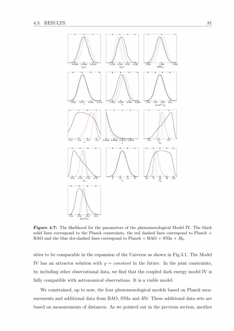
4.3. RESULTS 81
0.0198 0.0204 0.0210
Ωbh2
0.120 0.126 0.132 0.138
Ωch2
1.038 1.040 1.042100θMC
0.050 0.075 0.100 0.125τ
0.915 0.930 0.945 0.960ns
3.00 3.04 3.08 3.12
ln(1010As)
−2.4 −2.0 −1.6 −1.2w
0.0000 0.0008 0.0016 0.0024ξ
0.6 0.7 0.8ΩΛ
0.16 0.24 0.32 0.40Ωm
8 10 12 14zre
60 70 80 90 100H0
13.6 13.8 14.0 14.2
Age/Gyr
Figure 4.7: The likelihood for the parameters of the phenomenological Model IV. The blacksolid lines correspond to the Planck constraints, the red dashed lines correspond to Planck +BAO and the blue dot-dashed lines correspond to Planck + BAO + SNIa + H0.
sities to be comparable in the expansion of the Universe as shown in Fig.3.1. The Model
IV has an attractor solution with % ∼ constant in the future. In the joint constraints,
by including other observational data, we find that the coupled dark energy model IV is
fully compatible with astronomical observations. It is a viable model.
We constrained, up to now, the four phenomenological models based on Planck mea-
surements and additional data from BAO, SNIa and H0. These additional data sets are
based on measurements of distances. As we pointed out in the previous section, another
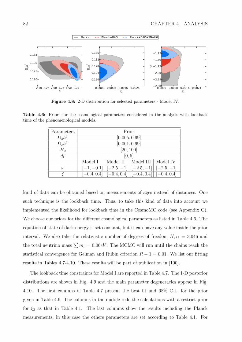
82 CHAPTER 4. ANALYSIS
−2.50−2.25−2.00−1.75−1.50−1.25w
0.120
0.125
0.130
0.135
Ωch
2
0.0000 0.0008 0.0016 0.0024ξ1
0.120
0.124
0.128
0.132
0.136
Ωch
20.0000 0.0008 0.0016 0.0024
ξ1
−2.50
−2.25
−2.00
−1.75
−1.50
−1.25
w
Planck Planck+BAO Planck+BAO+SN+H0
Figure 4.8: 2-D distribution for selected parameters - Model IV.
Table 4.6: Priors for the cosmological parameters considered in the analysis with lookbacktime of the phenomenological models.
Parameters PriorΩbh
2 [0.005, 0.99]Ωch
2 [0.001, 0.99]H0 [20, 100]df [0, 5]
Model I Model II Model III Model IV
ω [−1,−0.1] [−2.5,−1] [−2.5,−1] [−2.5,−1]
ξ [−0.4, 0.4] [−0.4, 0.4] [−0.4, 0.4] [−0.4, 0.4]
kind of data can be obtained based on measurements of ages instead of distances. One
such technique is the lookback time. Thus, to take this kind of data into account we
implemented the likelihood for lookback time in the CosmoMC code (see Appendix C).
We choose our priors for the different cosmological parameters as listed in Table 4.6. The
equation of state of dark energy is set constant, but it can have any value inside the prior
interval. We also take the relativistic number of degrees of freedom Neff = 3.046 and
the total neutrino mass∑mν = 0.06eV . The MCMC will run until the chains reach the
statistical convergence for Gelman and Rubin criterion R − 1 = 0.01. We list our fitting
results in Tables 4.7-4.10. These results will be part of publication in [100].
The lookback time constraints for Model I are reported in Table 4.7. The 1-D posterior
distributions are shown in Fig. 4.9 and the main parameter degeneracies appear in Fig.
4.10. The first columns of Table 4.7 present the best fit and 68% C.L. for the prior
given in Table 4.6. The columns in the middle redo the calculations with a restrict prior
for ξ2 as that in Table 4.1. The last columns show the results including the Planck
measurements, in this case the others parameters are set according to Table 4.1. For

4.3. RESULTS 83
Table 4.7: Cosmological parameters - LBT analysis for Model I.
LBT+H0 LBT+H0 (ξ2 = [−0.4, 0]) LBT+H0+PlanckParameter Best fit 68% limits Best fit 68% limits Best fit 68% limits
Ωbh2 0.1693 0.09288+0.0277
−0.0879 0.009321 0.03423+0.00737−0.0292 0.02185 0.02203+0.000252
−0.000251
Ωch2 0.05315 0.08679+0.0244
−0.0858 0.006469 0.03003+0.00751−0.029 0.04167 0.04524+0.0168
−0.04
H0 73.22 73.15+2.42−2.42 72.85 72.94+2.44
−2.5 71.69 71.06+1.82−1.82
w -0.6778 −0.7319+0.143−0.165 -0.4277 −0.7098+0.184
−0.141 -0.9621 −0.9346+0.016−0.0644
ξ2 0.2708 0.1992+0.197−0.0635 -0.008092 −0.05135+0.0513
−0.00763 -0.2048 −0.1878+0.0479−0.0812
df 2.461 2.205+0.31−0.259 2.387 1.831+0.27
−0.268 1.376 1.381+0.0993−0.0991
Ωd 0.5838 0.6623+0.0794−0.154 0.969 0.8772+0.0623
−0.0465 0.8751 0.8637+0.0784−0.0389
Ωm 0.4162 0.3377+0.154−0.08 0.03097 0.1228+0.047
−0.0627 0.1249 0.1363+0.0389−0.0784
χ2min/2 13.48 13.60 4921.61
0.06 0.12 0.18 0.24
Ωbh2
0.06 0.12 0.18 0.24
Ωch2
65 70 75 80H0
−0.8 −0.6 −0.4w
−0.2 0.0 0.2ξ2
1.2 1.8 2.4 3.0df
0.45 0.60 0.75 0.90Ωd
0.00 0.15 0.30 0.45 0.60Ωm
Figure 4.9: The likelihood for the parameters of the phenomenological Model I using lookbacktime measurements. The black solid lines correspond to the LBT + H0 constraints, the reddashed lines correspond to LBT + H0 with a restricted prior to ξ2 = [−0.4, 0] and the bluedot-dashed lines correspond to LBT + H0 + Planck.
lookback time calculations of Model I, we use the age of the Universe obtained with
Planck data tobs0 = 13.821Gyr with one standard deviation σtobs0= 0.101Gyr. From the
fitting results, we observe that Planck measurements provide narrower constraints than
lookback time, especially for Ωbh2. This would be expected since baryon perturbations are
coupled to photons and thus the CMB anisotropies depend on the amount of baryons. On
the other hand, lookback time only takes into account the background evolution. We also
see that lookback time prefers a dark energy equation of state in the quintessence regime
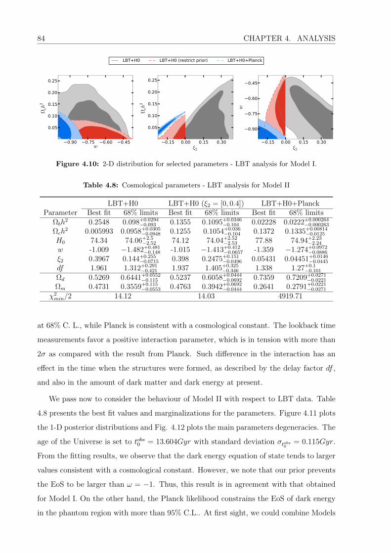
84 CHAPTER 4. ANALYSIS
−0.90 −0.75 −0.60 −0.45w
0.05
0.10
0.15
0.20
0.25
Ωch
2
−0.15 0.00 0.15 0.30ξ2
0.05
0.10
0.15
0.20
0.25
Ωch
2−0.15 0.00 0.15 0.30
ξ2
−0.90
−0.75
−0.60
−0.45
w
LBT+H0 LBT+H0 (restrict prior) LBT+H0+Planck
Figure 4.10: 2-D distribution for selected parameters - LBT analysis for Model I.
Table 4.8: Cosmological parameters - LBT analysis for Model II
LBT+H0 LBT+H0 (ξ2 = [0, 0.4]) LBT+H0+PlanckParameter Best fit 68% limits Best fit 68% limits Best fit 68% limits
Ωbh2 0.2548 0.098+0.0294
−0.093 0.1355 0.1095+0.0346−0.104 0.02228 0.0222+0.000264
−0.000263
Ωch2 0.005993 0.0958+0.0305
−0.0948 0.1255 0.1054+0.036−0.104 0.1372 0.1335+0.00814
−0.0125
H0 74.34 74.06+2.5−2.52 74.12 74.04+2.52
−2.53 77.88 74.94+2.23−2.24
w -1.009 −1.482+0.481−0.148 -1.015 −1.413+0.412
−0.0657 -1.359 −1.274+0.0972−0.0886
ξ2 0.3967 0.144+0.255−0.0715 0.398 0.2475+0.151
−0.0496 0.05431 0.04451+0.0146−0.0445
df 1.961 1.312+0.291−0.421 1.937 1.405+0.325
−0.346 1.338 1.27+0.1−0.101
Ωd 0.5269 0.6441+0.0552−0.115 0.5237 0.6058+0.0444
−0.0692 0.7359 0.7209+0.0271−0.0221
Ωm 0.4731 0.3559+0.115−0.0553 0.4763 0.3942+0.0692
−0.0444 0.2641 0.2791+0.0221−0.0271
χ2min/2 14.12 14.03 4919.71
at 68% C. L., while Planck is consistent with a cosmological constant. The lookback time
measurements favor a positive interaction parameter, which is in tension with more than
2σ as compared with the result from Planck. Such difference in the interaction has an
effect in the time when the structures were formed, as described by the delay factor df ,
and also in the amount of dark matter and dark energy at present.
We pass now to consider the behaviour of Model II with respect to LBT data. Table
4.8 presents the best fit values and marginalizations for the parameters. Figure 4.11 plots
the 1-D posterior distributions and Fig. 4.12 plots the main parameters degeneracies. The
age of the Universe is set to tobs0 = 13.604Gyr with standard deviation σtobs0= 0.115Gyr.
From the fitting results, we observe that the dark energy equation of state tends to larger
values consistent with a cosmological constant. However, we note that our prior prevents
the EoS to be larger than ω = −1. Thus, this result is in agreement with that obtained
for Model I. On the other hand, the Planck likelihood constrains the EoS of dark energy
in the phantom region with more than 95% C.L.. At first sight, we could combine Models
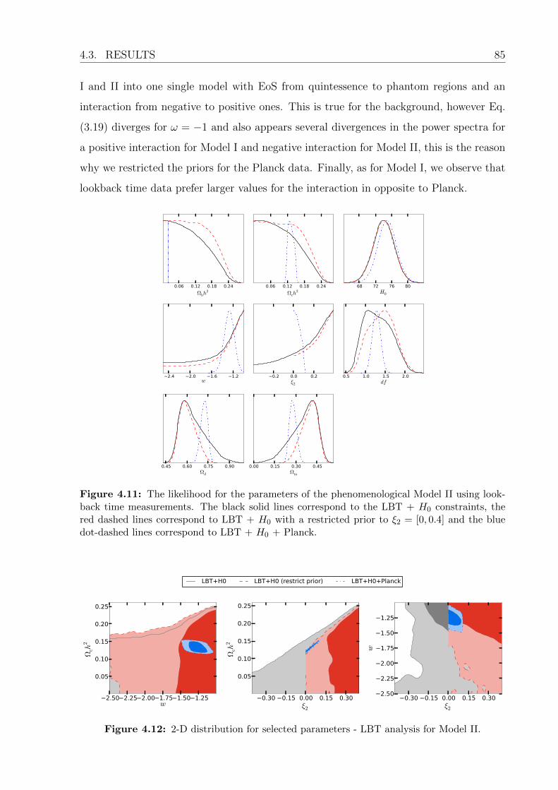
4.3. RESULTS 85
I and II into one single model with EoS from quintessence to phantom regions and an
interaction from negative to positive ones. This is true for the background, however Eq.
(3.19) diverges for ω = −1 and also appears several divergences in the power spectra for
a positive interaction for Model I and negative interaction for Model II, this is the reason
why we restricted the priors for the Planck data. Finally, as for Model I, we observe that
lookback time data prefer larger values for the interaction in opposite to Planck.
0.06 0.12 0.18 0.24
Ωbh2
0.06 0.12 0.18 0.24
Ωch2
68 72 76 80H0
−2.4 −2.0 −1.6 −1.2w
−0.2 0.0 0.2ξ2
0.5 1.0 1.5 2.0df
0.45 0.60 0.75 0.90Ωd
0.00 0.15 0.30 0.45Ωm
Figure 4.11: The likelihood for the parameters of the phenomenological Model II using look-back time measurements. The black solid lines correspond to the LBT + H0 constraints, thered dashed lines correspond to LBT + H0 with a restricted prior to ξ2 = [0, 0.4] and the bluedot-dashed lines correspond to LBT + H0 + Planck.
−2.50−2.25−2.00−1.75−1.50−1.25w
0.05
0.10
0.15
0.20
0.25
Ωch
2
−0.30 −0.15 0.00 0.15 0.30ξ2
0.05
0.10
0.15
0.20
0.25
Ωch
2
−0.30 −0.15 0.00 0.15 0.30ξ2
−2.50
−2.25
−2.00
−1.75
−1.50
−1.25
w
LBT+H0 LBT+H0 (restrict prior) LBT+H0+Planck
Figure 4.12: 2-D distribution for selected parameters - LBT analysis for Model II.

86 CHAPTER 4. ANALYSIS
Table 4.9: Cosmological parameters - LBT analysis for Model III
LBT+H0 LBT+H0 (ξ1 = [0, 0.4]) LBT+H0+PlanckParameter Best fit 68% limits Best fit 68% limits Best fit 68% limits
Ωbh2 0.006805 0.0378+0.00592
−0.0328 0.009584 0.03848+0.0059−0.0335 0.02248 0.02244+0.000332
−0.000399
Ωch2 0.3828 0.252+0.106
−0.0793 0.386 0.2503+0.105−0.0759 0.1199 0.1251+0.00331
−0.00462
H0 73.1 73.69+2.65−2.6 73.25 73.65+2.61
−2.59 74.27 74.26+2.46−2.46
w -1.64 −1.731+0.73−0.769 -1.558 −1.722+0.721
−0.778 -1.232 −1.417+0.212−0.112
ξ1 0.3735 0.3033+0.0957−0.0199 0.3955 0.3054+0.0936
−0.0215 0.0006722 0.002171+0.000729−0.00197
df 2.506 2.048+0.379−0.298 2.554 2.048+0.369
−0.287 1.669 1.405+0.181−0.146
Ωd 0.2698 0.4615+0.156−0.138 0.2616 0.4628+0.152
−0.134 0.7406 0.7305+0.0218−0.0177
Ωm 0.7302 0.5385+0.138−0.156 0.7384 0.5372+0.134
−0.152 0.2594 0.2695+0.0177−0.0218
χ2min/2 11.59 11.59 4918.55
Table 4.10: Cosmological parameters - LBT analysis for Model IV
LBT+H0 LBT+H0 (ξ = [0, 0.4]) LBT+H0+PlanckParameter Best fit 68% limits Best fit 68% limits Best fit 68% limits
Ωbh2 0.007615 0.04137+0.00758
−0.0364 0.005097 0.0409+0.00713−0.0359 0.0224 0.0224+0.000335
−0.000376
Ωch2 0.4325 0.3159+0.103
−0.0854 0.3857 0.3177+0.106−0.0835 0.125 0.1251+0.00302
−0.00316
H0 73.27 73.22+2.59−2.59 72.89 73.17+2.52
−2.54 73.83 74.03+2.29−2.6
w -2.384 −1.702+0.701−0.798 -1.768 −1.702+0.701
−0.798 -1.341 −1.384+0.167−0.113
ξ 0.3188 0.3011+0.0979−0.0247 0.2772 0.3014+0.0976
−0.0238 0.00141 0.001953+0.000914−0.00116
df 2.498 2.188+0.411−0.356 2.406 2.192+0.422
−0.362 1.378 1.323+0.115−0.116
Ωd 0.1791 0.3287+0.155−0.153 0.2632 0.3251+0.157
−0.155 0.7284 0.7289+0.0191−0.0167
χ2min/2 13.39 13.39 4920.34
Models III and IV present very similar behavior. The best fit values and 68% C.L.
limits are presented in Tables 4.9 and 4.10 for Models III and IV, respectively. Figures
4.13 and 4.14 show the 1-D posterior distributions for the parameters, while Fig. 4.15 and
Fig. 4.16 plot the main parameter degeneracies. For Model III the age of the Universe is
given by tobs0 = 13.928Gyr with standard deviation σtobs0= 0.280 and for Model IV the age
is tobs0 = 13.854Gyr and σtobs0= 0.111, which were obtained from the Planck measurements
alone. We observe that Planck measurements pin the parameters down much better than
lookback time data for both models, especially the dark energy equation of state which is
completely unconstrained using LBT. There is still a tension in the determination of the
interaction parameter over several sigmas, e.g. the 95% C.L. lower limit for the interaction
using only LBT is ξ1 = 0.14 for Model III, while the maximum value at 95% C.L. with
Planck is ξ1 = 0.0047. Note the tiny confidence regions for Planck constraints as compared
with the LBT constraints, and the separation between them in the 2-D distributions.

4.3. RESULTS 87
0.04 0.08 0.12 0.16
Ωbh2
0.15 0.30 0.45
Ωch2
65 70 75 80H0
−2.4 −2.0 −1.6 −1.2w
−0.15 0.00 0.15 0.30ξ1
1.2 1.8 2.4 3.0df
0.00 0.25 0.50 0.75Ωd
0.25 0.50 0.75 1.00Ωm
Figure 4.13: The likelihood for the parameters of the phenomenological Model III using look-back time measurements. The black solid lines correspond to the LBT + H0 constraints, thered dashed lines correspond to LBT + H0 with a restricted prior to ξ1 = [0, 0.4] and the bluedot-dashed lines correspond to LBT + H0 + Planck.
0.04 0.08 0.12 0.16
Ωbh2
0.15 0.30 0.45 0.60
Ωch2
65 70 75 80H0
−2.4 −2.0 −1.6 −1.2w
0.0 0.1 0.2 0.3ξ
1.2 1.8 2.4 3.0df
0.0 0.3 0.6Ωd
Figure 4.14: The likelihood for the parameters of the phenomenological Model IV using look-back time measurements. The black solid lines correspond to the LBT + H0 constraints, thered dashed lines correspond to LBT + H0 with a restricted prior to ξ = [0, 0.4] and the bluedot-dashed lines correspond to LBT + H0 + Planck .
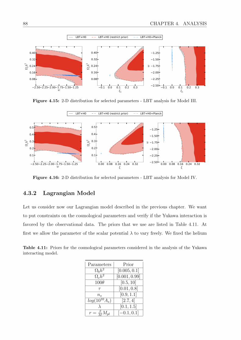
88 CHAPTER 4. ANALYSIS
−2.50−2.25−2.00−1.75−1.50−1.25w
0.08
0.16
0.24
0.32
0.40
Ωch
2
−0.1 0.0 0.1 0.2 0.3ξ1
0.08
0.16
0.24
0.32
0.40
Ωch
2−0.1 0.0 0.1 0.2 0.3
ξ1
−2.50
−2.25
−2.00
−1.75
−1.50
−1.25
w
LBT+H0 LBT+H0 (restrict prior) LBT+H0+Planck
Figure 4.15: 2-D distribution for selected parameters - LBT analysis for Model III.
−2.50−2.25−2.00−1.75−1.50−1.25w
0.1
0.2
0.3
0.4
0.5
Ωch
2
0.00 0.08 0.16 0.24 0.32ξ
0.1
0.2
0.3
0.4
0.5
Ωch
2
0.00 0.08 0.16 0.24 0.32ξ
−2.50
−2.25
−2.00
−1.75
−1.50
−1.25
w
LBT+H0 LBT+H0 (restrict prior) LBT+H0+Planck
Figure 4.16: 2-D distribution for selected parameters - LBT analysis for Model IV.
4.3.2 Lagrangian Model
Let us consider now our Lagrangian model described in the previous chapter. We want
to put constraints on the cosmological parameters and verify if the Yukawa interaction is
favored by the observational data. The priors that we use are listed in Table 4.11. At
first we allow the parameter of the scalar potential λ to vary freely. We fixed the helium
Table 4.11: Priors for the cosmological parameters considered in the analysis of the Yukawainteracting model.
Parameters PriorΩbh
2 [0.005, 0.1]Ωch
2 [0.001, 0.99]100θ [0.5, 10]τ [0.01, 0.8]ns [0.9, 1.1]
log(1010As) [2.7, 4]λ [0.1, 1.5]
r = βMMpl [−0.1, 0.1]

4.3. RESULTS 89
Table 4.12: Cosmological parameters - Lagrangian Model
Planck Planck+BAO Planck+BAO+SNIa+H0Parameter Best fit 68% limits Best fit 68% limits Best fit 68% limits
Ωbh2 0.02203 0.02196+0.000278
−0.000279 0.02225 0.02204+0.000252−0.000264 0.02222 0.02211+0.000263
−0.000261
Ωch2 0.1185 0.119+0.00277
−0.00283 0.1181 0.1176+0.00211−0.00181 0.1171 0.1165+0.00185
−0.00166
100θMC 1.041 1.041+0.000625−0.000623 1.042 1.041+0.000564
−0.000567 1.042 1.041+0.000572−0.000565
τ 0.09723 0.0883+0.0118−0.0136 0.09281 0.09063+0.0123
−0.0125 0.08889 0.09231+0.0126−0.0127
ns 0.9625 0.9579+0.00702−0.00701 0.9631 0.9608+0.00592
−0.00577 0.9647 0.9629+0.00573−0.00558
ln(1010As) 3.101 3.084+0.0229−0.0256 3.091 3.086+0.0239
−0.0243 3.086 3.087+0.0249−0.0247
λ 0.6777 0.7451+0.755−0.645 0.227 0.6046+0.151
−0.505 0.3007 0.3904+0.0736−0.29
r -0.02182 −0.001969+0.0224−0.0224 -0.003793 −0.0008486+0.0238
−0.0281 0.01311 −0.002299+0.033−0.0338
Ωd 0.6858 0.6744+0.0236−0.0213 0.6942 0.688+0.0141
−0.0116 0.699 0.701+0.0103−0.0101
Ωm 0.3142 0.3256+0.0213−0.0236 0.3058 0.312+0.0116
−0.0141 0.301 0.299+0.0101−0.0103
zre 11.67 10.93+1.04−1.05 11.22 11.07+1.04
−1.07 10.87 11.17+1.07−1.07
H0 67.04 66.05+1.93−1.77 67.91 67.09+1.3
−0.968 68.19 68.28+0.849−0.839
Age/Gyr 13.81 13.84+0.0651−0.0567 13.79 13.81+0.0414
−0.0417 13.78 13.77+0.0438−0.0407
χ2min/2 4902.91 4903.89 4972.01
0.25 0.50 0.75 1.00 1.25 1.50λ
0.110
0.115
0.120
0.125
Ωch
2
−0.050−0.0250.000 0.025 0.050r
0.110
0.115
0.120
0.125
Ωch
2
−0.050−0.0250.000 0.025 0.050r
0.25
0.50
0.75
1.00
1.25
1.50
λ
Planck Planck+BAO Planck+BAO+SN+H0
Figure 4.17: 2-D distribution for selected parameters - Lagrangian Model.
abundance as Yp = 0.24. The number of relativistic degrees of freedom is adjusted to
Neff = 3.046 and the total neutrino mass is set to∑mν = 0.06eV . At last the spectrum
lensing normalization is AL = 1. To finish the MCMC we set the Gelman and Rubin
criterion to R− 1 = 0.03. The results obtained for this model will be published soon [99].
To constrain the Yukawa-type interacting dark energy, we use the measurements of the
CMB anisotropies made by Planck together with BAO, SNIa andH0 measurements. Using
the priors listed in Table 4.11 we run the MCMC. The results are shown in Table 4.12, the
1-D posteriors for the parameters are given in Fig. 4.18 and some parameter degeneracies
are in Fig. 4.17. We observe that the Planck data alone is not able to constrain the
scalar potential λ and it constrains the interaction parameter r symmetrically around the
zero value. This is what we expected from the discussion about the power spectra of the
Lagrangian model in the previous chapter, as illustrated in Figs. 3.6 and 3.7. Adding low

90 CHAPTER 4. ANALYSIS
redshift measurements, λ tends to its lower limit, while the interaction parameter slightly
breaks the symmetry around the zero value. We see that allowing the scalar potential
vary freely does not favor an interacting model. In fact, it shows a tendency to λ → 0
and r = 0, which is basically the ΛCDM model.
0.0216 0.0224
Ωbh2
0.108 0.114 0.120 0.126
Ωch2
1.040 1.042
100θMC
0.050 0.075 0.100 0.125
τ
0.930 0.945 0.960 0.975
ns
3.00 3.05 3.10 3.15
ln(1010As)
0.3 0.6 0.9 1.2 1.5
λ−0.04 0.00 0.04
r
0.60 0.65 0.70 0.75
Ωd
0.25 0.30 0.35 0.40
Ωm
8 10 12 14
zre
63 66 69 72
H0
13.6 13.7 13.8 13.9 14.0
Age/Gyr
Figure 4.18: The likelihood for the parameters of the Lagrangian Model. The black solid linescorrespond to the Planck constraints, the red dashed lines correspond to Planck + BAO andthe blue dot-dashed lines correspond to Planck + BAO + SNIa + H0.
We then consider the case when we fix the scalar potential parameter λ. We have
learned that as we increase the value for λ, the interaction becomes more favored. For
instance, λ =√
3/2 produces the results in Table 4.13 and the 1-D posterior distributions

4.3. RESULTS 91
Table 4.13: Cosmological parameters - Lagrangian Model with Fixed λ
Planck Planck+BAO Planck+BAO+SNIa+H0Parameter Best fit 68% limits Best fit 68% limits Best fit 68% limits
Ωbh2 0.02177 0.02195+0.000276
−0.000274 0.02203 0.02208+0.000265−0.000263 0.02216 0.02218+0.000272
−0.000267
Ωch2 0.1203 0.1192+0.00288
−0.00282 0.1186 0.1166+0.0026−0.00202 0.117 0.1155+0.00238
−0.00182
100θMC 1.041 1.041+0.000621−0.000618 1.041 1.041+0.000581
−0.000569 1.042 1.042+0.00059−0.000598
τ 0.08242 0.08848+0.0117−0.0144 0.0964 0.09183+0.0124
−0.0142 0.1005 0.09495+0.0127−0.0145
ns 0.9557 0.9575+0.00727−0.00734 0.961 0.9629+0.00619
−0.00607 0.9666 0.9662+0.00609−0.00599
ln(1010As) 3.076 3.085+0.0226−0.0271 3.099 3.086+0.0243
−0.0271 3.103 3.09+0.0252−0.0281
r -0.02151 −0.001283+0.0208−0.0243 -0.01445 −0.005535+0.021
−0.0343 -0.03228 −0.02173+0.0105−0.0346
Ωd 0.654 0.6567+0.0161−0.0163 0.6632 0.6731+0.0108
−0.0109 0.6804 0.6851+0.0101−0.0101
Ωm 0.346 0.3433+0.0163−0.0161 0.3368 0.3269+0.0109
−0.0108 0.3196 0.3149+0.0101−0.0101
zre 10.51 10.95+1.06−1.17 11.61 11.14+1.1
−1.08 11.85 11.33+1.1−1.09
H0 64.23 64.31+0.943−1.06 64.77 65.31+0.729
−0.72 66.14 66.29+0.744−0.866
Age/Gyr 13.89 13.87+0.053−0.0455 13.86 13.83+0.0422
−0.0424 13.78 13.78+0.0506−0.045
χ2min/2 4903.15 4905.40 4977.26
Table 4.14: Cosmological parameters - LBT analysis for the Lagrangian Model
LBT+H0 LBT+H0+PlanckParameter Best fit 68% limits Best fit 68% limits
Ωbh2 0.01379 0.04993+0.0501
−0.0449 0.02193 0.02202+0.000223−0.000227
Ωch2 0.05908 0.04989+0.0211
−0.0407 0.1177 0.1173+0.00213−0.00212
H0 73.85 74.25+2.39−2.38 67.73 67.57+0.989
−0.978
λ 1.495 1.091+0.409−0.0893 0.1664 0.482+0.106
−0.382
r 0.04726 0.001707+0.0983−0.102 -0.01 −0.001682+0.0226
−0.0279
df 2.025 1.819+0.21−0.264 1.307 1.339+0.0923
−0.0924
Ωd 0.8652 0.8159+0.0415−0.0439 0.6942 0.6932+0.0136
−0.0122
Ωm 0.1348 0.1841+0.0438−0.0415 0.3058 0.3068+0.0122
−0.0136
χ2min/2 14.62 4924.29
are plotted in Fig. 4.19. These results show that even when we fix the parameter λ, the
Planck data alone is compatible with a null interaction. However, if we include low redshift
measurements from BAO, SNIa and H0, the symmetric value of r is broken and it favors
a negative value of r. For this value of λ, the negative interaction parameter is favored
at 68% C.L.. Augmenting the value of λ, a negative r is even more favorable. Thus, we
conclude that if we are able to determine the value of λ, or if we have a theoretical model
fixing it, if this value is sufficiently large, the Yukawa interaction between dark energy
and dark matter will be preferred by the cosmological data.
At last we analyze the Lagrangian model comparing it with the lookback time data.
The results are in Table 4.14. Figures 4.20 and 4.21 present the 1-D posteriors and the
main parameter degeneracies, respectively. As expected, the lookback time yields much
broader results as compared with the Planck constraints. It is not able to constrain the

92 CHAPTER 4. ANALYSIS
0.0216 0.0224 0.0232
Ωbh2
0.108 0.114 0.120 0.126
Ωch2
1.040 1.042
100θMC
0.06 0.09 0.12 0.15
τ
0.945 0.960 0.975 0.990
ns
3.00 3.05 3.10 3.15
ln(1010As)
−0.08 −0.04 0.00 0.04
r
0.60 0.64 0.68 0.72
Ωd
0.30 0.33 0.36 0.39
Ωm
8 10 12 14
zre
62 64 66 68
H0
13.6 13.7 13.8 13.9 14.0
Age/Gyr
Figure 4.19: The likelihood for the parameters of the Lagrangian Model with fixed λ. Theblack solid lines correspond to the Planck constraints, the red dashed lines correspond to Planck+ BAO and the blue dot-dashed lines correspond to Planck + BAO + SNIa + H0.
interaction, which is completely undetermined with lookback time data alone. From the
posterior distributions, we observe that LBT data prefer larger values of λ, which is in the
opposite direction to the Planck measurements. Fixing the value of λ does not improve
the LBT constraints for the interaction parameter, thus we do not present the results for
this case here. We conclude that the LBT data alone are not of much help to constrain
the Lagrangian Model with Yukawa-type interaction, but they show a tension with the
Planck data in the determination of the scalar potential parameter. These results are
part of a publication to appear soon[100].
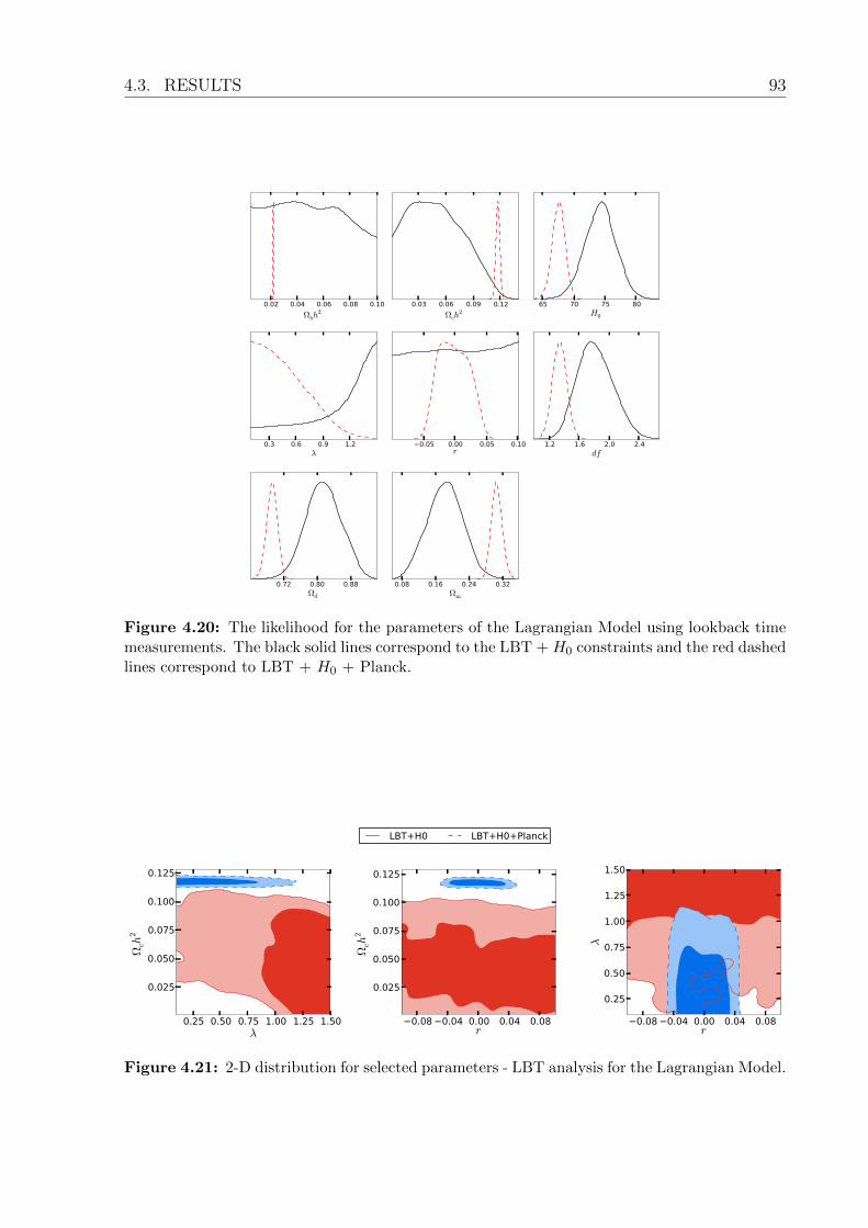
4.3. RESULTS 93
0.02 0.04 0.06 0.08 0.10
Ωbh2
0.03 0.06 0.09 0.12
Ωch2
65 70 75 80H0
0.3 0.6 0.9 1.2λ
−0.05 0.00 0.05 0.10r
1.2 1.6 2.0 2.4df
0.72 0.80 0.88Ωd
0.08 0.16 0.24 0.32Ωm
Figure 4.20: The likelihood for the parameters of the Lagrangian Model using lookback timemeasurements. The black solid lines correspond to the LBT + H0 constraints and the red dashedlines correspond to LBT + H0 + Planck.
0.25 0.50 0.75 1.00 1.25 1.50λ
0.025
0.050
0.075
0.100
0.125
Ωch
2
−0.08−0.04 0.00 0.04 0.08r
0.025
0.050
0.075
0.100
0.125
Ωch
2
−0.08−0.04 0.00 0.04 0.08r
0.25
0.50
0.75
1.00
1.25
1.50
λ
LBT+H0 LBT+H0+Planck
Figure 4.21: 2-D distribution for selected parameters - LBT analysis for the Lagrangian Model.

Conclusions
The aim of this thesis was to propose models of interaction between dark energy and dark
matter and discover from observational data if the interaction is favored.
Chapter one dealt with basic aspects of cosmology. We introduced the simple homo-
geneous and isotropic model for the Universe and the equations governing its evolution.
Then, in order to put the cosmological models on experimental basis, we described def-
initions of cosmic distances which allow us to constrain the cosmological parameters of
a model from observations and make predictions that can be falsifiable. For instance,
observations of surpernova type Ia put constraints from luminosity distances and mea-
surements of baryon acustic oscillations are based on angular diameter distances. Finally,
we discussed how current observations lead to the necessity of two unknown components:
dark matter and dark energy.
The structures around us imply that we must go beyond the homogeneous and isotropic
universe if our model intends to explain the real Universe. On large scales, we can im-
prove our model through small perturbations in the background. Chapter two introduced
such perturbations and developed their dynamical equations. The linear perturbations
over the smooth background lead to predictions about the cosmic microwave background
anisotropies and matter inhomogeneities which can be tested by anisotropy probes, e.g.
Planck satellite, and galaxy surveys, respectively.
The first two chapters were concerned to establish the cosmological basis we needed.
In chapter three we explore the possibility of an interaction in the dark sector. The sim-
plest cosmological model, the ΛCDM, is in good agreement with current observations.
However, it suffers from two theoretical problems: the cosmological constant problem
and the coincidence problem. Thus, we consider alternative models: the first is a phe-
nomenological model with an interaction given by a linear combination of the dark fluids
Q = 3H(ξ1ρc + ξ2ρd); and, as a tentative to build a more fundamental framework, the
94
95
second model comes from a Lagrangian density of a scalar field, describing dark energy,
and a fermionic field, for dark matter, with an Yukawa interaction between them.
The last chapter compares the theoretical predictions of the interacting models with
several observational data. The data show that an interaction is allowed and in some
cases it is favored. We also observe some tension between the results from Planck with
the low redshift measurements from lookback time. The lookback time favors a larger
positive interaction for the phenomenological models, while for the Planck data it is more
consistent with zero and even negative values for Model I. On the other hand, the lookback
time data prefer larger values for the scalar potential parameter λ of the Lagrangian model,
in the opposite direction to the Planck results. Appendices A, B and C present the most
important parts of the computational implementation used in this thesis.
From this thesis we see at least two possible directions for future works: first, there
is still much space for alternative models of dark energy and dark matter, and different
kinds of interaction; second, there are other data sets that were not considered here and
new techniques and probes should be taken into account. These studies will certainly
augment our knowledge of the nature of dark matter and dark energy.
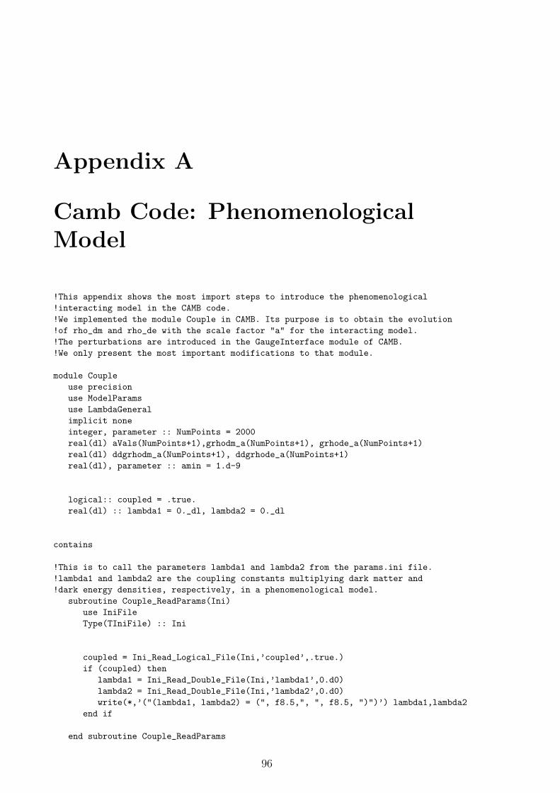
Appendix A
Camb Code: PhenomenologicalModel
!This appendix shows the most import steps to introduce the phenomenological
!interacting model in the CAMB code.
!We implemented the module Couple in CAMB. Its purpose is to obtain the evolution
!of rho_dm and rho_de with the scale factor "a" for the interacting model.
!The perturbations are introduced in the GaugeInterface module of CAMB.
!We only present the most important modifications to that module.
module Couple
use precision
use ModelParams
use LambdaGeneral
implicit none
integer, parameter :: NumPoints = 2000
real(dl) aVals(NumPoints+1),grhodm_a(NumPoints+1), grhode_a(NumPoints+1)
real(dl) ddgrhodm_a(NumPoints+1), ddgrhode_a(NumPoints+1)
real(dl), parameter :: amin = 1.d-9
logical:: coupled = .true.
real(dl) :: lambda1 = 0._dl, lambda2 = 0._dl
contains
!This is to call the parameters lambda1 and lambda2 from the params.ini file.
!lambda1 and lambda2 are the coupling constants multiplying dark matter and
!dark energy densities, respectively, in a phenomenological model.
subroutine Couple_ReadParams(Ini)
use IniFile
Type(TIniFile) :: Ini
coupled = Ini_Read_Logical_File(Ini,’coupled’,.true.)
if (coupled) then
lambda1 = Ini_Read_Double_File(Ini,’lambda1’,0.d0)
lambda2 = Ini_Read_Double_File(Ini,’lambda2’,0.d0)
write(*,’("(lambda1, lambda2) = (", f8.5,", ", f8.5, ")")’) lambda1,lambda2
end if
end subroutine Couple_ReadParams
96
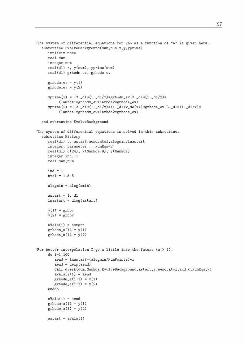
97
!The system of differential equations for rho as a function of "a" is given here.
subroutine EvolveBackground(dum,num,x,y,yprime)
implicit none
real dum
integer num
real(dl) x, y(num), yprime(num)
real(dl) grhodm_ev, grhode_ev
grhodm_ev = y(1)
grhode_ev = y(2)
yprime(1) = -3._dl*(1._dl/x)*grhodm_ev+3._dl*(1._dl/x)*
(lambda1*grhodm_ev+lambda2*grhode_ev)
yprime(2) = -3._dl*(1._dl/x)*(1._dl+w_de(x))*grhode_ev-3._dl*(1._dl/x)*
(lambda1*grhodm_ev+lambda2*grhode_ev)
end subroutine EvolveBackground
!The system of differential equations is solved in this subroutine.
subroutine History
real(dl) :: astart,aend,atol,alogmin,lnastart
integer, parameter :: NumEqs=2
real(dl) c(24), w(NumEqs,9), y(NumEqs)
integer ind, i
real dum,num
ind = 1
atol = 1.d-5
alogmin = dlog(amin)
astart = 1._dl
lnastart = dlog(astart)
y(1) = grhoc
y(2) = grhov
aVals(1) = astart
grhodm_a(1) = y(1)
grhode_a(1) = y(2)
!For better interpolation I go a little into the future (a > 1).
do i=1,100
aend = lnastart-(alogmin/NumPoints)*i
aend = dexp(aend)
call dverk(dum,NumEqs,EvolveBackground,astart,y,aend,atol,ind,c,NumEqs,w)
aVals(i+1) = aend
grhodm_a(i+1) = y(1)
grhode_a(i+1) = y(2)
enddo
aVals(1) = aend
grhodm_a(1) = y(1)
grhode_a(1) = y(2)
astart = aVals(1)

98 APPENDIX A. CAMB CODE: PHENOMENOLOGICAL MODEL
lnastart = dlog(astart)
do i=1, NumPoints
aend = lnastart+(alogmin/NumPoints)*i
aend = dexp(aend)
call dverk(dum,NumEqs,EvolveBackground,astart,y,aend,atol,ind,c,NumEqs,w)
aVals(i+1) = aend
grhodm_a(i+1) = y(1)
grhode_a(i+1) = y(2)
enddo
call Flip(aVals)
call Flip(grhodm_a)
call Flip(grhode_a)
do i=1, NumPoints+1
aVals(i)=dlog(aVals(i))
enddo
call spline(aVals,grhodm_a,NumPoints+1,1.d30,1.d30,ddgrhodm_a)
call spline(aVals,grhode_a,NumPoints+1,1.d30,1.d30,ddgrhode_a)
end subroutine History
!This subroutine is to invert the order of the splines.
subroutine Flip(xdat)
real(dl) :: xdat(NumPoints),swap_x
integer i,pos
do i=1, NumPoints+1
pos = (NumPoints+1)-i
if (pos > i) then
swap_x = xdat(pos)
xdat(pos) = xdat(i)
xdat(i) = swap_x
endif
end do
end subroutine
!rho_dm as a function of "a".
function grhodm(a) !8 pi G rho_dm
real(dl) :: grhodm, al
real(dl), intent(IN) :: a
al=dlog(a)
if(al.lt.aVals(1)) then
grhodm=grhodm_a(1) !if a < minimum a from wa.dat
else
if(al.gt.aVals(NumPoints)) then
grhodm=grhodm_a(NumPoints) !if a > maximus a from wa.dat
else
call cubicsplint(aVals,grhodm_a,ddgrhodm_a,NumPoints,al,grhodm)
endif
endif
end function grhodm
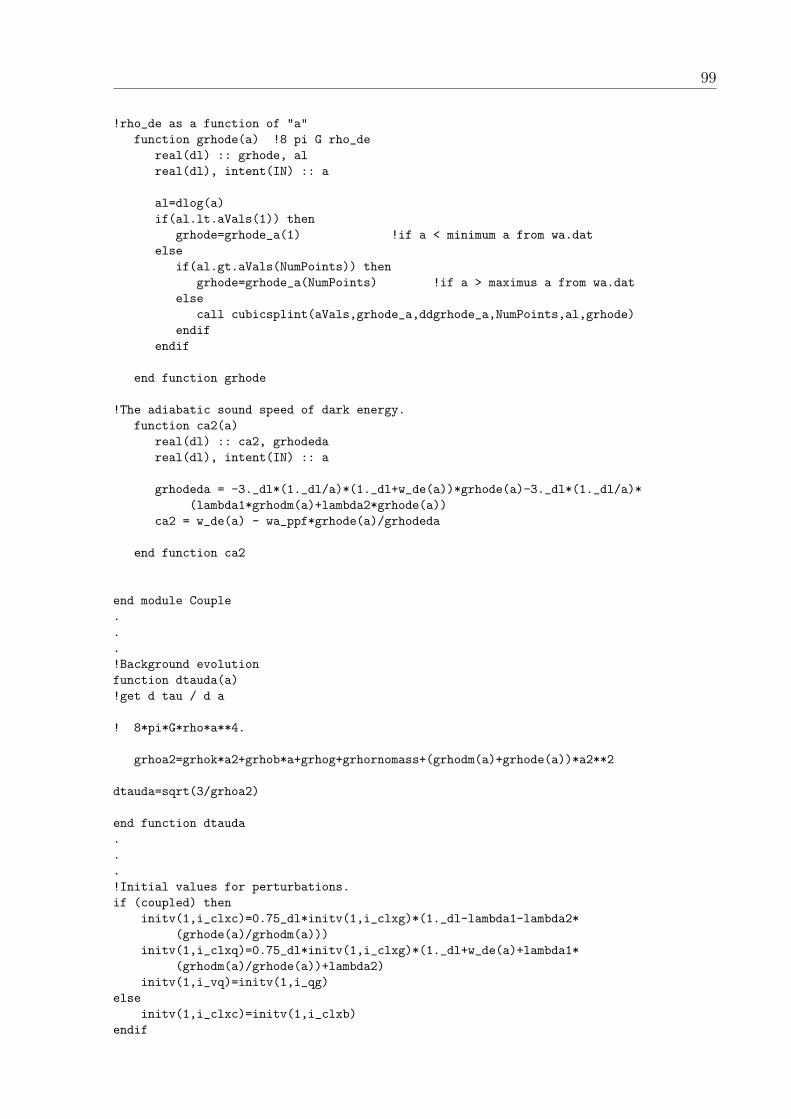
99
!rho_de as a function of "a"
function grhode(a) !8 pi G rho_de
real(dl) :: grhode, al
real(dl), intent(IN) :: a
al=dlog(a)
if(al.lt.aVals(1)) then
grhode=grhode_a(1) !if a < minimum a from wa.dat
else
if(al.gt.aVals(NumPoints)) then
grhode=grhode_a(NumPoints) !if a > maximus a from wa.dat
else
call cubicsplint(aVals,grhode_a,ddgrhode_a,NumPoints,al,grhode)
endif
endif
end function grhode
!The adiabatic sound speed of dark energy.
function ca2(a)
real(dl) :: ca2, grhodeda
real(dl), intent(IN) :: a
grhodeda = -3._dl*(1._dl/a)*(1._dl+w_de(a))*grhode(a)-3._dl*(1._dl/a)*
(lambda1*grhodm(a)+lambda2*grhode(a))
ca2 = w_de(a) - wa_ppf*grhode(a)/grhodeda
end function ca2
end module Couple
.
.
.
!Background evolution
function dtauda(a)
!get d tau / d a
! 8*pi*G*rho*a**4.
grhoa2=grhok*a2+grhob*a+grhog+grhornomass+(grhodm(a)+grhode(a))*a2**2
dtauda=sqrt(3/grhoa2)
end function dtauda
.
.
.
!Initial values for perturbations.
if (coupled) then
initv(1,i_clxc)=0.75_dl*initv(1,i_clxg)*(1._dl-lambda1-lambda2*
(grhode(a)/grhodm(a)))
initv(1,i_clxq)=0.75_dl*initv(1,i_clxg)*(1._dl+w_de(a)+lambda1*
(grhodm(a)/grhode(a))+lambda2)
initv(1,i_vq)=initv(1,i_qg)
else
initv(1,i_clxc)=initv(1,i_clxb)
endif

100 APPENDIX A. CAMB CODE: PHENOMENOLOGICAL MODEL
.
.
.
grhoc_t=grhodm(a)*a2
grhov_t=grhode(a)*a2
w_eff = w_de(a)
!total perturbations: matter terms first, then add massive nu, de and radiation
! 8*pi*a*a*SUM[rho_i*clx_i]
dgrho=grhob_t*clxb+grhoc_t*clxc
! 8*pi*a*a*SUM[(rho_i+p_i)*v_i]
dgq=grhob_t*vb
clxq=ay(EV%w_ix)
vq=ay(EV%w_ix+1)
dgrho=dgrho + clxq*grhov_t
dgq = dgq + vq*grhov_t*(1._dl+w_eff)
.
.
.
!Perturbed dark energy equation of motion
if (coupled) then
ayprime(Ev%w_ix)= 3._dl*adotoa*w_eff*clxq + &
3._dl*adotoa*lambda1*(grhoc_t/grhov_t)*(clxq - clxc)&
- (1._dl+w_eff)*k*vq - 3._dl*adotoa*cs2_lam*clxq - &
3._dl*adotoa*(cs2_lam-ca2(a))*(3._dl*adotoa*(1._dl+w_eff) + &
3._dl*adotoa*(lambda1*(grhoc_t/grhov_t) + lambda2))*&
vq/k - (1._dl+w_eff)*k*z
ayprime(Ev%w_ix+1)= -adotoa*(1._dl-3._dl*cs2_lam)*vq + &
(3._dl*adotoa/(1._dl+w_eff))*(1._dl+cs2_lam)*&
(lambda1*(grhoc_t/grhov_t) + lambda2)*vq + &
cs2_lam*k*clxq/(1._dl+w_eff)
! CDM equation of motion
clxcdot= -k*z + 3._dl*adotoa*lambda2*(grhov_t/grhoc_t)*(clxq - clxc)
ayprime(3) = clxcdot
else
clxcdot=-k*z
ayprime(3)=clxcdot
endif
Appendix B
Camb Code: Lagrangian Model
!This appendix shows the most import steps to introduce the lagrangian
!interacting model in the CAMB code.
!We implemented the module QCouple in CAMB. Its purpose is to obtain the evolution
!of rho_dm, phi and phidot with the scale factor a for the interacting model.
!The perturbations are introduced in the GaugeInterface module of CAMB.
!We only present the most important modifications to that module.
module QCouple
use precision
use Errors
use ModelParams
use LambdaGeneral
implicit none
integer, parameter :: NumPoints = 2000, NumPointsEx = NumPoints+2
real(dl) aVals(NumPointsEx), grhodm_a(NumPointsEx), phi_a(NumPointsEx),
phidot_a(NumPointsEx)
real(dl) ddgrhodm_a(NumPointsEx), ddphi_a(NumPointsEx), ddphidot_a(NumPointsEx)
real(dl) initial_grhoc, initial_phi, initial_phidot, adot, y_grhoc, norm_grhoc
real(dl), parameter :: amin = 1.d-9
real(dl) :: lambda = 0._dl, r_int = 0._dl, rphi = -1.d0
logical :: OK_int = .true.
contains
!This is to call the parameters lambda and r_int from the params.ini file.
!lambda is the power of the potential V(psi) and r_int is the coupling constant
!divided by the dark matter mass, respectively.
subroutine Couple_ReadParams(Ini)
use IniFile
Type(TIniFile) :: Ini
if (coupled) then
lambda = Ini_Read_Double_File(Ini,’lambda’,0.d0)
r_int = Ini_Read_Double_File(Ini,’r_int’,0.d0)
rphi = Ini_Read_Double_File(Ini,’rphi’,-1.d0)
write(*,’("(lambda, r_int, rphi) = (", f8.5,", ", f8.5, ", ", f8.5, ")")’)
lambda, r_int, rphi
end if
101
102 APPENDIX B. CAMB CODE: LAGRANGIAN MODEL
end subroutine Couple_ReadParams
function Vofphi(phi,deriv)
!Returns (8*Pi*G)^(1-deriv/2)*d^derivV(psi)/d^derivpsi evaluated at psi
!times (Mpc/c)^2 to get units in 1/Mpc^2
!The input variable phi is sqrt(8*Pi*G)*psi
use constants
implicit none
real(dl) phi, Vofphi
integer deriv
real(dl) norm
!Normalized so that lambda=0 and r_int=0 gives norm=grhov
norm = 3._dl*CP%H0**2*(1000)**2/c**2*CP%omegav
if (deriv==0) then
Vofphi = norm*exp(-lambda*phi)
else
if (deriv==1) then
Vofphi = -lambda*norm*exp(-lambda*phi)
else
if (deriv==2) then
Vofphi = lambda**2*norm*exp(-lambda*phi)
else
stop ’Invalid deriv in Vofphi’
endif
endif
endif
end function Vofphi
!The system of differential equations for rho as a function of "a" is given here.
subroutine EvolveBackground(dum,num,x,y,yprime)
use constants
use MassiveNu
implicit none
real dum
integer num
real(dl) x, y(num), yprime(num)
real(dl) x2, grhodm_ev, phi, phidot, ga2T00_de, ga2T00, dphida, Q_int
real(dl) rhonu
integer nu_i
OK_int = .true.
x2 = x**2
phi = y(1)
phidot = y(2)/x2
if (x == amin) then
norm_grhoc = y_grhoc*amin**3/(1-r_int*phi)
endif
grhodm_ev = norm_grhoc/x**3*(1 - r_int*phi)

103
y_grhoc = grhodm_ev
if (rphi < 0) then
if (r_int*phi < 1._dl) then
Q_int = -r_int/(1._dl - r_int*phi)
else
grhodm_ev = 0._dl
Q_int = 0
OK_int = .false.
endif
else
if (r_int*phi > 1._dl) then
Q_int = -r_int/(1._dl - r_int*phi)
else
grhodm_ev = 0._dl
Q_int = 0
OK_int = .false.
endif
endif
ga2T00_de = x2*(0.5d0*phidot**2 + x2*Vofphi(phi,0))
ga2T00 = grhok*x2+grhob*x+grhog+grhornomass+grhodm_ev*x2**2+ga2T00_de
if (CP%Num_Nu_massive /= 0) then
!Get massive neutrino density relative to massless
do nu_i = 1, CP%nu_mass_eigenstates
call Nu_rho(x*nu_masses(nu_i),rhonu)
ga2T00 = ga2T00 +rhonu*grhormass(nu_i)
end do
end if
adot = sqrt(ga2T00/3.0d0)
dphida = phidot/adot
yprime(1) = dphida
yprime(2) = -x2**2*(Vofphi(phi,1) + Q_int*grhodm_ev)/adot
end subroutine EvolveBackground
function GetOmegaFromInitial(astart,grhoc_initial,phi,phidot,atol)
!Get CP%omegac and CP%omegav today given particular conditions grhoc, phi and
!phidot at a=astart
implicit none
real(dl), intent(IN) :: astart, grhoc_initial, phi, phidot, atol
real(dl), dimension(2) :: GetOmegaFromInitial
integer, parameter :: NumEqs=2
real(dl) c(24), w(NumEqs,9), y(NumEqs), ast
integer ind, i
real dum
ast=astart
ind=2
104 APPENDIX B. CAMB CODE: LAGRANGIAN MODEL
do i=1,9
c(i)=0._dl
enddo
c(4)=1d-30
c(5)=100
y_grhoc = grhoc_initial
y(1) = phi
y(2) = phidot*astart**2 !Fixed Dec 02
call dverk(dum,NumEqs,EvolveBackground,ast,y,1._dl,atol,ind,c,NumEqs,w)
if (OK_int) then
call EvolveBackground(dum,NumEqs,1._dl,y,w(:,1))
GetOmegaFromInitial(1) = y_grhoc/(3*adot**2)
GetOmegaFromInitial(2) = (0.5d0*y(2)**2 + Vofphi(y(1),0))/(3*adot**2)
else
return
endif
!Search for initial phi.
subroutine GetInitialPhi(trial_grhoc,error_phi)
implicit none
real(dl) astart
real(dl) atol
real(dl) initial_phi2
real(dl), dimension(2):: om
real(dl) :: omv1, omv2, deltaphi, phi, trial_grhoc, initial_phi_inv
real(dl) :: omv_min, initial_phi_min, omv_max, initial_phi_max, phi1, phi2
integer, optional :: error_phi
logical OK
integer:: iter = 0, iter2
iter2 = 0
omv_min = 1000
omv_max = -1000
astart = amin
!These two must bracket the correct value to give CP%omegav today
!Assume that higher initial phi gives higher CP%omegav today
!Can fix initial_phi to correct value
if (rphi < 0) then
if (r_int > 0) then
initial_phi = 1._dl/r_int - 1._dl/(100*r_int)
initial_phi2 = -100/lambda
else
if (r_int < 0) then
initial_phi = 100/lambda
initial_phi2 = 1._dl/r_int - 1._dl/(100*r_int)
else
initial_phi = 100/lambda
initial_phi2 = -100/lambda
endif
endif
else

105
if (r_int < 0) then
initial_phi = 1._dl/r_int + 1._dl/(100*r_int)
initial_phi2 = -100/lambda
else
if (r_int > 0) then
initial_phi = 100/lambda
initial_phi2 = 1._dl/r_int + 1._dl/(100*r_int)
else
initial_phi = 100/lambda
initial_phi2 = -100/lambda
endif
endif
endif
if (CP%omegav < 0) then
initial_phi_inv = initial_phi
initial_phi = initial_phi2
initial_phi2 = initial_phi_inv
endif
initial_phidot = 0._dl
atol = 1d-5
!See if initial conditions are giving correct CP%omegav now
om = GetOmegaFromInitial(astart,trial_grhoc,initial_phi,initial_phidot,atol)
if (OK_int .and. om(2) < CP%omegav) then
omv1 = om(2)
else
do while (OK_int == .false. .or. om(2) > CP%omegav)
iter2 = iter2 + 1
phi = initial_phi + (initial_phi2 - initial_phi)/2
om = GetOmegaFromInitial(astart,trial_grhoc,phi,initial_phidot,atol)
if (om(2) < CP%omegav .or. OK_int == .false.) then
initial_phi = phi
else
initial_phi2 = phi
endif
if (om(2) < omv_min .and. OK_int) then
omv_min = om(2)
initial_phi_min = phi
endif
if (iter2 == 50 .and. omv_min > CP%omegav) then
do iter2 = 1, 10
phi1 = initial_phi_min + 1
phi2 = initial_phi_min - 1
om = GetOmegaFromInitial(astart,trial_grhoc,phi1,initial_phidot,atol)
omv1 = om(2) - CP%omegav
om = GetOmegaFromInitial(astart,trial_grhoc,phi2,initial_phidot,atol)
omv2 = om(2) - CP%omegav
phi = phi2 - (phi2 - phi1)*omv2/(omv2 - omv1)
om = GetOmegaFromInitial(astart,trial_grhoc,phi,initial_phidot,atol)
if (OK_int) then

106 APPENDIX B. CAMB CODE: LAGRANGIAN MODEL
phi1 = phi2
phi2 = phi
else
phi1 = phi
endif
if (om(2) < omv_min .and. OK_int) then
omv_min = om(2)
initial_phi_min = phi
endif
if (om(2) <= CP%omegav .and. OK_int) then
initial_phi = phi
exit
endif
if (iter2 == 10) then
om(2) = omv_min
initial_phi = initial_phi_min
endif
enddo
exit
endif
enddo
omv1 = om(2)
endif
if (abs(omv1-CP%omegav) > 1d-5) then
!if not, do binary search in the interval
OK = .false.
iter2 = 0
om = GetOmegaFromInitial(astart,trial_grhoc,initial_phi2,initial_phidot,atol)
if (OK_int .and. om(2) > CP%omegav) then
omv2 = om(2)
else
do while (OK_int == .false. .or. om(2) < CP%omegav)
iter2 = iter2 + 1
phi = initial_phi2 + (initial_phi - initial_phi2)/2
om = GetOmegaFromInitial(astart,trial_grhoc,phi,initial_phidot,atol)
if (om(2) > CP%omegav .or. OK_int == .false.) then
initial_phi2 = phi
else
initial_phi = phi
endif
omv2 = om(2)
if (om(2) > omv_max .and. OK_int) then
omv_max = om(2)
initial_phi_max = phi
endif
if (iter2 == 50 .and. omv_max < CP%omegav) then
do iter2 = 1, 10
phi1 = initial_phi_max + 1
phi2 = initial_phi_max - 1
om = GetOmegaFromInitial(astart,trial_grhoc,phi1,initial_phidot,

107
atol)
omv1 = om(2) - CP%omegav
om = GetOmegaFromInitial(astart,trial_grhoc,phi2,initial_phidot,atol)
omv2 = om(2) - CP%omegav
phi = phi1 - (phi1 - phi2)*omv1/(omv1 - omv2)
om = GetOmegaFromInitial(astart,trial_grhoc,phi,initial_phidot,atol)
if (OK_int) then
phi2 = phi1
phi1 = phi
else
phi2 = phi
endif
if (om(2) > omv_max .and. OK_int) then
omv_max = om(2)
initial_phi_max = phi
endif
if (om(2) >= CP%omegav .and. OK_int) then
initial_phi2 = phi
exit
endif
if (iter2 == 10) then
om(2) = omv_max
initial_phi2 = initial_phi_max
endif
enddo
exit
endif
enddo
omv2 = om(2)
endif
if (omv1 > CP%omegav .or. omv2 < CP%omegav) then
if (error_phi == 100) then
write (*,*) ’Initial phi values must bracket required value.’
call GlobalError(’Initial phi values must bracket required value.’,
error_evolution)
else
return
endif
end if
do iter = 1,100
deltaphi = initial_phi2 - initial_phi
phi = initial_phi + deltaphi/2
om = GetOmegaFromInitial(astart,trial_grhoc,phi,initial_phidot,atol)
if (OK_int) then
if (om(2) < CP%omegav) then
omv1 = om(2)
initial_phi = phi
else
omv2 = om(2)
initial_phi2 = phi
end if
else

108 APPENDIX B. CAMB CODE: LAGRANGIAN MODEL
if (phi >= initial_phi) then
initial_phi = phi
else
initial_phi2 = phi
endif
endif
if (omv2 - omv1 < 1d-5) then
OK = .true.
initial_phi = (initial_phi2 + initial_phi)/2
exit
end if
end do
if (.not. OK .and. error_phi == 100) then !this shouldn’t happen
write (*,*) ’Search for good phi initial condition did not converge.’
call GlobalError(’Search for good phi initial condition did not converge.’,
error_evolution)
endif
endif
end subroutine GetInitialPhi
!Search for initial grhoc.
subroutine Init_background
implicit none
real(dl) astart
real(dl) atol
real(dl) initial_grhoc2
real(dl), dimension(2):: om
real(dl) omc1, omc2, deltagrhoc, rhoc
logical OK
integer:: iter = 0
astart = amin
atol = 1d-5
if (lambda == 0._dl .and. r_int == 0._dl) then
!These two must bracket the correct value to give CP%omegac today
!Assume that higher initial grhoc gives higher CP%omegac today
!Can fix initial_grhoc to correct value
initial_grhoc = 1d1*grhoc/astart**3
initial_grhoc2 = 1d-1*grhoc/astart**3
initial_phi = 10
initial_phidot = 0._dl
!See if initial conditions are giving correct CP%omegac now
om = GetOmegaFromInitial(astart,initial_grhoc,initial_phi,initial_phidot,atol)
omc1 = om(1)
if (abs(omc1-CP%omegac) > 1d-4) then
!if not, do binary search in the interval
OK = .false.
om = GetOmegaFromInitial(astart,initial_grhoc2,initial_phi,initial_phidot,atol)
109
omc2 = om(1)
if (omc1 < CP%omegac .or. omc2 > CP%omegac) then
write (*,*) ’Initial grhoc values must bracket required value.’
call GlobalError(’Initial grhoc values must bracket required value.’,
error_evolution)
end if
do iter = 1,100
deltagrhoc = initial_grhoc2 - initial_grhoc
rhoc = initial_grhoc + deltagrhoc/2
om = GetOmegaFromInitial(astart,rhoc,initial_phi,initial_phidot,atol)
if (om(1) > CP%omegac) then
omc1 = om(1)
initial_grhoc = rhoc
else
omc2 = om(1)
initial_grhoc2 = rhoc
end if
if (omc1 - omc2 < 1d-5 .and. abs(om(2)-CP%omegav) < 1d-4) then
OK = .true.
initial_grhoc = (initial_grhoc2 + initial_grhoc)/2
if (FeedbackLevel > 0) write(*,*) ’grhoc_initial = ’, initial_grhoc
if (FeedbackLevel > 0) write(*,*) ’phi_initial = ’, initial_phi
om = GetOmegaFromInitial(astart,initial_grhoc,initial_phi,initial_phidot,
atol)
if (FeedbackLevel > 0) write(*,*) ’Omegac0, Omegac = ’, om(1), CP%omegac
if (FeedbackLevel > 0) write(*,*) ’Omegav0, Omegav = ’, om(2), CP%omegav
exit
end if
end do
if (.not. OK) then !this shouldn’t happen
write (*,*) ’Search for good initial conditions did not converge.’
call GlobalError(’Search for good initial conditions did not converge.’,
error_evolution)
endif
endif
else
!These two must bracket the correct value to give CP%omegac today
!Assume that higher initial grhoc gives higher CP%omegac today
!Can fix initial_grhoc to correct value
initial_grhoc = 1d3*grhoc/astart**3
initial_grhoc2 = 1d-3*grhoc/astart**3
!See if initial conditions are giving correct CP%omegac now
call GetInitialPhi(initial_grhoc,0)
om = GetOmegaFromInitial(astart,initial_grhoc,initial_phi,initial_phidot,atol)
if (OK_int .and. om(1) > CP%omegac) then
omc1 = om(1)
else
do iter = 1,10
initial_grhoc = initial_grhoc/2

110 APPENDIX B. CAMB CODE: LAGRANGIAN MODEL
call GetInitialPhi(initial_grhoc,0)
om = GetOmegaFromInitial(astart,initial_grhoc,initial_phi,initial_phidot,
atol)
if (OK_int .and. om(1) > CP%omegac) then
omc1 = om(1)
exit
endif
enddo
omc1 = om(1)
endif
if (abs(omc1-CP%omegac) > 1d-5) then
!if not, do binary search in the interval
OK = .false.
call GetInitialPhi(initial_grhoc2,0)
om = GetOmegaFromInitial(astart,initial_grhoc2,initial_phi,initial_phidot,
atol)
if (OK_int .and. om(1) < CP%omegac) then
omc2 = om(1)
else
do iter = 1,10
initial_grhoc2 = 2*initial_grhoc2
call GetInitialPhi(initial_grhoc2,0)
om = GetOmegaFromInitial(astart,initial_grhoc2,initial_phi,
initial_phidot,atol)
if (OK_int .and. om(1) < CP%omegac) then
omc2 = om(1)
exit
endif
enddo
omc2 = om(1)
endif
if (omc1 < CP%omegac .or. omc2 > CP%omegac) then
write (*,*) ’Initial grhoc values must bracket required value.’
call GlobalError(’Initial grhoc values must bracket required value.’,
error_evolution)
end if
do iter = 1,100
deltagrhoc = initial_grhoc2 - initial_grhoc
rhoc = initial_grhoc + deltagrhoc/2
call GetInitialPhi(rhoc,iter)
om = GetOmegaFromInitial(astart,rhoc,initial_phi,initial_phidot,atol)
if (om(1) > CP%omegac) then
omc1 = om(1)
initial_grhoc = rhoc
else
omc2 = om(1)
initial_grhoc2 = rhoc
end if
if (omc1 - omc2 < 1d-5 .and. abs(om(2)-CP%omegav) < 1d-4) then
OK = .true.
initial_grhoc = (initial_grhoc2 + initial_grhoc)/2
if (FeedbackLevel > 0) write(*,*) ’grhoc_initial = ’, initial_grhoc

111
if (FeedbackLevel > 0) write(*,*) ’phi_initial = ’, initial_phi
om = GetOmegaFromInitial(astart,initial_grhoc,initial_phi,
initial_phidot,atol)
if (FeedbackLevel > 0) write(*,*) ’Omegac0, Omegac =’,om(1),CP%omegac
if (FeedbackLevel > 0) write(*,*) ’Omegav0, Omegav =’,om(2),CP%omegav
exit
end if
end do
if (.not. OK) then !this shouldn’t happen
write (*,*) ’Search for good initial conditions did not converge.’
call GlobalError(’Search for good initial conditions did not converge.’,
error_evolution)
endif
endif
endif
end subroutine Init_background
!Here we make interpolation tables.
subroutine History
implicit none
real(dl) :: astart, afrom, aend
integer, parameter :: NumEqs=2
real(dl) c(24), w(NumEqs,9), y(NumEqs), atol, splZero
integer ind, i
real dum
ind = 1
atol = 1.d-5
astart = amin
afrom = astart
call Init_background
y_grhoc = initial_grhoc
y(1) = initial_phi
y(2) = initial_phidot
aVals(1) = astart
grhodm_a(1) = y_grhoc
phi_a(1) = y(1)
phidot_a(1) = y(2)
!For better interpolation I go a little into the future (a > 1).
do i=1, NumPointsEx-1
aend = dlog(astart)-(dlog(astart)/(NumPoints-1))*i
aend = dexp(aend)
call dverk(dum,NumEqs,EvolveBackground,afrom,y,aend,atol,ind,c,NumEqs,w)
call EvolveBackground(dum,NumEqs,aend,y,w(:,1))
aVals(i+1) = aend
112 APPENDIX B. CAMB CODE: LAGRANGIAN MODEL
grhodm_a(i+1) = y_grhoc
phi_a(i+1) = y(1)
phidot_a(i+1) = y(2)
if (i==NumPoints-1) then
if (FeedbackLevel > 0) then
write(*,*) ’Omega_Q_0=’,real((0.5d0*phidot_a(i+1)**2 +
Vofphi(phi_a(i+1),0))/(3*adot**2)), &
’ w_0=’,real((0.5d0*phidot_a(i+1)**2 - Vofphi(phi_a(i+1),0))/
(0.5d0*phidot_a(i+1)**2 + Vofphi(phi_a(i+1),0)))
end if
end if
enddo
splZero = 0
call spline(aVals,grhodm_a,NumPointsEx,splZero,splZero,ddgrhodm_a)
call spline(aVals,phi_a,NumPointsEx,splZero,splZero,ddphi_a)
call spline(aVals,phidot_a,NumPointsEx,splZero,splZero,ddphidot_a)
end subroutine History
!rho_dm as a function of "a".
function grhodm(a) !8 pi G rho_dm
real(dl) :: grhodm
real(dl), intent(IN) :: a
if(a.lt.aVals(1)) then
grhodm=grhodm_a(1) !if a < minimum
else
if(a.gt.aVals(NumPointsEx)) then
grhodm=grhodm_a(NumPointsEx) !if a > maximus
else
call cubicsplint(aVals,grhodm_a,ddgrhodm_a,NumPointsEx,a,grhodm)
endif
endif
end function grhodm
!phi as a function of "a"
function fphi(a) !sqrt(8*pi*G)*psi
real(dl) :: fphi
real(dl), intent(IN) :: a
if(a.lt.aVals(1)) then
fphi=phi_a(1) !if a < minimum
else
if(a.gt.aVals(NumPointsEx)) then
fphi=phi_a(NumPointsEx) !if a > maximus
else
call cubicsplint(aVals,phi_a,ddphi_a,NumPointsEx,a,fphi)
endif
endif
end function fphi

113
!phidot as a function of "a"
function fphidot(a) !sqrt(8*pi*G)*psidot
real(dl) :: fphidot
real(dl), intent(IN) :: a
if(a.lt.aVals(1)) then
fphidot=phidot_a(1) !if a < minimum
else
if(a.gt.aVals(NumPointsEx)) then
fphidot=phidot_a(NumPointsEx) !if a > maximus
else
call cubicsplint(aVals,phidot_a,ddphidot_a,NumPointsEx,a,fphidot)
endif
endif
end function fphidot
end module QCouple
.
.
.
!Background evolution
function dtauda(a)
!get d tau / d a
! 8*pi*G*rho*a**4.
phi = fphi(a)
grhoa2=grhok*a2+grhob*a+grhog+grhornomass+grhodm(a)*a2**2+
(0.5d0*fphidot(a)**2 + a2*Vofphi(phi,0))*a2
dtauda=sqrt(3/grhoa2)
end function dtauda
.
.
.
!Initial values for perturbations.
if (coupled) then
initv(1,i_clxc)=0.75_dl*initv(1,i_clxg)
i_phi = fphi(a)
i_phidot = fphidot(a)
i_Vofphi = Vofphi(i_phi,0)
if (lambda /= 0) then
initv(1,i_clxq)=(2._dl*initv(1,i_clxc)*i_phidot**2*i_Vofphi)/
((i_phidot**2 + 2._dl*a2*i_Vofphi)*Vofphi(i_phi,1))
else
initv(1,i_clxq)=0._dl
endif
initv(1,i_vq)=(initv(1,i_clxc)*i_phidot**3)/(i_phidot**2 + 2._dl*a2*i_Vofphi)
initv(1,i_vc)=0._dl
else
initv(1,i_clxc)=initv(1,i_clxb)
endif
114 APPENDIX B. CAMB CODE: LAGRANGIAN MODEL
.
.
.
grhoc_t=grhodm(a)*a2
phia=fphi(a)
phidota=fphidot(a)
Vofphia=Vofphi(phia,0)
grhov_t=0.5d0*phidota**2 + a2*Vofphia
w_eff = (0.5d0*phidota**2 - Vofphia)/(0.5d0*phidota**2 + Vofphia)
!total perturbations: matter terms first, then add massive nu, de and radiation
! 8*pi*a*a*SUM[rho_i*clx_i]
dgrho=grhob_t*clxb+grhoc_t*clxc
! 8*pi*a*a*SUM[(rho_i+p_i)*v_i]
dgq=grhob_t*vb+grhoc_t*vc
clxq=ay(EV%w_ix)
vq=ay(EV%w_ix+1)
dgrho=dgrho + phidota*vq + a2*Vofphi(phia,1)*clxq
dgq = dgq + k*phidota*clxq
.
.
.
!Perturbed dark energy equation of motion
if (coupled) then
Q_inter = -r_int/(1._dl - r_int*phia)
Q_phiphi = r_int**2/(1._dl - r_int*phia)**2
ayprime(Ev%w_ix)= vq
ayprime(Ev%w_ix+1)= -2._dl*adotoa*vq - k2*clxq - a2*Vofphi(phia,2)*clxq &
- k*z*phidota - a2*(Q_phiphi)&
*clxq*grhoc_t/a2 - a2*(Q_inter)&
*(grhoc_t/a2)*clxc
! CDM equation of motion
clxcdot= -k*z - k*vc + (Q_inter)*vq + &
(Q_phiphi)*phidota*clxq
ayprime(3) = clxcdot
ayprime(Ev%w_ix+2)= -adotoa*vc - (Q_inter)*phidota*vc&
+ k*(Q_inter)*clxq
else
clxcdot=-k*z
ayprime(3)=clxcdot
endif
Appendix C
CosmoMC Code: Lookback Time
!This appendix shows the most import steps to introduce the lookback time
!likelihood in the CosmoMC code.
module LBT
use cmbtypes
use CAMB, only: Hofz, DeltaPhysicalTimeGyr
use constants
use Precision
use likelihood
implicit none
real(dl) Age_universe_theory, Age_universe_obs, Age_universe_err
type, extends(CosmologyLikelihood) :: LBTLikelihood
integer :: num_lbt !total number of points used
real(dl), allocatable, dimension(:) :: lbt_z, lbt_age, lbt_err
real(dl), allocatable, dimension(:,:) :: lbt_invcov
contains
procedure :: LogLike => LBT_LnLike
end type LBTLikelihood
contains
!This is to add the Lookback Time Likelihood
subroutine LBTLikelihood_Add(LikeList, Ini)
use IniFile
use settings
class(LikelihoodList) :: LikeList
Type(TIniFile) :: ini
Type(LBTLikelihood), pointer :: like
integer numlbtsets, i
if (Ini_Read_Logical_File(Ini, ’use_LBT’,.false.)) then
Age_universe_obs = Ini_Read_Double_File(Ini,’Age_universe_obs’,0.d0)
Age_universe_err = Ini_Read_Double_File(Ini,’Age_universe_err’,0.d0)
numlbtsets = Ini_Read_Int_File(Ini,’lbt_numdatasets’,0)
if (numlbtsets<1) call MpiStop(’Use_LBT but numlbtsets = 0’)
115

116 APPENDIX C. COSMOMC CODE: LOOKBACK TIME
do i= 1, numlbtsets
allocate(like)
call ReadLBTDataset(like, ReadIniFileName(Ini,numcat(’lbt_dataset’,i)) )
like%LikelihoodType = ’LBT’
like%needs_background_functions = .true.
call like%loadParamNames(trim(DataDir)//’LBT.paramnames’)
call LikeList%Add(like)
end do
if (Feedback>1) write(*,*) ’read lookback time datasets’
end if
end subroutine LBTLikelihood_Add
!This is to read the Lookback Time data
subroutine ReadLBTDataset(bset, gname)
use MatrixUtils
type (LBTLikelihood) bset
character(LEN=*), intent(IN) :: gname
character(LEN=Ini_max_string_len) :: lbt_measurements_file, lbt_invcov_file
integer i,iopb
logical bad
Type(TIniFile) :: Ini
integer file_unit
file_unit = new_file_unit()
call Ini_Open_File(Ini, gname, file_unit, bad, .false.)
if (bad) then
write (*,*) ’Error opening data set file ’//trim(gname)
stop
end if
bset%name = Ini_Read_String_File(Ini,’name’)
Ini_fail_on_not_found = .false.
if (Feedback > 0) write (*,*) ’reading lookback time data set: ’//trim(bset%name)
bset%num_lbt = Ini_Read_Int_File(Ini,’num_lbt’,0)
if (bset%num_lbt.eq.0) write(*,*) ’ ERROR: parameter num_lbt not set’
allocate(bset%lbt_z(bset%num_lbt))
allocate(bset%lbt_age(bset%num_lbt))
allocate(bset%lbt_err(bset%num_lbt))
lbt_measurements_file = ReadIniFileName(Ini,’lbt_measurements_file’)
call OpenTxtFile(lbt_measurements_file, tmp_file_unit)
do i=1,bset%num_lbt
read (tmp_file_unit,*, iostat=iopb) bset%lbt_z(i),bset%lbt_age(i),bset%lbt_err(i)
end do
close(tmp_file_unit)
allocate(bset%lbt_invcov(bset%num_lbt,bset%num_lbt))
bset%lbt_invcov = 0
if(Ini_HasKey_File(Ini,lbt_invcov_file)) then
lbt_invcov_file = ReadIniFileName(Ini, ’lbt_invcov_file’)
call OpenTxtFile(lbt_invcov_file, tmp_file_unit)
do i=1, bset%num_lbt

117
read (tmp_file_unit,*,iostat=iopb) bset%lbt_invcov(i,:)
end do
close(tmp_file_unit)
if (iopb.ne.0) then
call MpiStop(’Error reading lookback time file ’//trim(lbt_invcov_file))
endif
else
do i=1,bset%num_lbt
bset%lbt_invcov(i,i) = 1._dl/(bset%lbt_err(i)**2 + Age_universe_err**2)
end do
endif
call Ini_Close_File(Ini)
call ClearFileUnit(file_unit)
end subroutine ReadLBTDataset
!Lookback Time integrand
function f_lbt(z)
! Type(CMBParams) CMB
real(dl), intent(in) :: z
real(dl) f_lbt
f_lbt = 1._dl/((1._dl + z)*Hofz(z))
end function f_lbt
!Lookback Time integral
function lookbacktime(z)
! Type(CMBParams) CMB
real(dl), intent(in) :: z
real(dl) rombint, lookbacktime, atol
external rombint
atol = 1d-5
lookbacktime = rombint(f_lbt,0.,z,atol)*Mpc/c/Gyr
end function lookbacktime
!Here we calculate the Lookback Time Likelihood
function LBT_LnLike(like, CMB, Theory, DataParams)
! use ModelParams
Class(LBTLikelihood) :: like
Class(CMBParams) CMB
Class(TheoryPredictions) Theory
real(mcp) :: DataParams(:)
integer j,k
real(mcp) LBT_LnLike
real(dl), allocatable :: LBT_theory(:), LBT_obs(:)
real(dl) sigma_lbt
LBT_LnLike=0
allocate(LBT_theory(like%num_lbt))
allocate(LBT_obs(like%num_lbt))
118 APPENDIX C. COSMOMC CODE: LOOKBACK TIME
Age_universe_theory = DeltaPhysicalTimeGyr(0._dl,1._dl)
sigma_lbt = DataParams(1)
do j=1, like%num_lbt
LBT_theory(j) = lookbacktime(like%lbt_z(j))
LBT_obs(j) = Age_universe_obs - like%lbt_age(j) - sigma_lbt
end do
do j=1, like%num_lbt
do k=1, like%num_lbt
LBT_LnLike = LBT_LnLike +&
(LBT_theory(j)-LBT_obs(j))*like%lbt_invcov(j,k)*&
(LBT_theory(k)-LBT_obs(k))
end do
end do
LBT_LnLike = LBT_LnLike + (Age_universe_theory - Age_universe_obs)**2/&
Age_universe_err**2
LBT_LnLike = LBT_LnLike/2.d0
deallocate(LBT_theory)
deallocate(LBT_obs)
end function LBT_LnLike
end module LBT
References
[1] S. Weinberg, Rev.Mod.Phys. 61, 1 (1989).
[2] L. P. Chimento, A. S. Jakubi, D. Pavon, and W. Zimdahl, Phys.Rev. D67, 083513(2003), arXiv:astro-ph/0303145 [astro-ph] .
[3] L. Amendola, Phys.Rev. D62, 043511 (2000), arXiv:astro-ph/9908023 [astro-ph] .
[4] L. Amendola and C. Quercellini, Phys.Rev. D68, 023514 (2003), arXiv:astro-ph/0303228 [astro-ph] .
[5] L. Amendola, S. Tsujikawa, and M. Sami, Phys.Lett. B632, 155 (2006),arXiv:astro-ph/0506222 [astro-ph] .
[6] D. Pavon and W. Zimdahl, Phys.Lett. B628, 206 (2005), arXiv:gr-qc/0505020 [gr-qc] .
[7] S. del Campo, R. Herrera, and D. Pavon, Phys.Rev. D78, 021302 (2008),arXiv:0806.2116 [astro-ph] .
[8] C. G. Boehmer, G. Caldera-Cabral, R. Lazkoz, and R. Maartens, Phys.Rev. D78,023505 (2008), arXiv:0801.1565 [gr-qc] .
[9] S. Chen, B. Wang, and J. Jing, Phys.Rev. D78, 123503 (2008), arXiv:0808.3482[gr-qc] .
[10] G. Olivares, F. Atrio-Barandela, and D. Pavon, Phys.Rev. D71, 063523 (2005),arXiv:astro-ph/0503242 [astro-ph] .
[11] G. Olivares, F. Atrio-Barandela, and D. Pavon, Phys.Rev. D77, 063513 (2008),arXiv:0706.3860 [astro-ph] .
[12] J. Valiviita, E. Majerotto, and R. Maartens, JCAP 0807, 020 (2008),arXiv:0804.0232 [astro-ph] .
[13] J.-H. He, B. Wang, and E. Abdalla, Phys.Lett. B671, 139 (2009), arXiv:0807.3471[gr-qc] .
[14] P. S. Corasaniti, Phys.Rev. D78, 083538 (2008), arXiv:0808.1646 [astro-ph] .
[15] B. M. Jackson, A. Taylor, and A. Berera, Phys.Rev. D79, 043526 (2009),arXiv:0901.3272 [astro-ph.CO] .
[16] D. Pavon and B. Wang, Gen.Rel.Grav. 41, 1 (2009), arXiv:0712.0565 [gr-qc] .
119

120 REFERENCES
[17] B. Wang, C.-Y. Lin, D. Pavon, and E. Abdalla, Phys.Lett. B662, 1 (2008),arXiv:0711.2214 [hep-th] .
[18] B. Wang, J. Zang, C.-Y. Lin, E. Abdalla, and S. Micheletti, Nucl.Phys. B778, 69(2007), arXiv:astro-ph/0607126 [astro-ph] .
[19] F. Simpson, B. M. Jackson, and J. A. Peacock, MNRAS, 411 (2): 1053 (2011),arXiv:1004.1920 [astro-ph.CO] .
[20] W. Zimdahl, Int.J.Mod.Phys. D14, 2319 (2005), arXiv:gr-qc/0505056 [gr-qc] .
[21] Z.-K. Guo, N. Ohta, and S. Tsujikawa, Phys.Rev. D76, 023508 (2007), arXiv:astro-ph/0702015 [ASTRO-PH] .
[22] C. Feng, B. Wang, E. Abdalla, and R.-K. Su, Phys.Lett. B665, 111 (2008),arXiv:0804.0110 [astro-ph] .
[23] J. Valiviita, R. Maartens, and E. Majerotto, Mon.Not.Roy.Astron.Soc. 402, 2355(2010), arXiv:0907.4987 [astro-ph.CO] .
[24] J.-Q. Xia, Phys.Rev. D80, 103514 (2009), arXiv:0911.4820 [astro-ph.CO] .
[25] J.-H. He, B. Wang, and P. Zhang, Phys.Rev. D80, 063530 (2009), arXiv:0906.0677[gr-qc] .
[26] M. Martinelli, L. Lopez Honorez, A. Melchiorri, and O. Mena, Phys.Rev. D81,103534 (2010), arXiv:1004.2410 [astro-ph.CO] .
[27] L. L. Honorez, B. A. Reid, O. Mena, L. Verde, and R. Jimenez, JCAP 1009, 029(2010), arXiv:1006.0877 [astro-ph.CO] .
[28] J.-H. He and B. Wang, JCAP 0806, 010 (2008), arXiv:0801.4233 [astro-ph] .
[29] J.-H. He, B. Wang, and Y. Jing, JCAP 0907, 030 (2009), arXiv:0902.0660 [gr-qc] .
[30] G. Caldera-Cabral, R. Maartens, and B. M. Schaefer, JCAP 0907, 027 (2009),arXiv:0905.0492 [astro-ph.CO] .
[31] J.-H. He, B. Wang, E. Abdalla, and D. Pavon, JCAP 1012, 022 (2010),arXiv:1001.0079 [gr-qc] .
[32] O. Bertolami, F. Gil Pedro, and M. Le Delliou, Phys.Lett. B654, 165 (2007),arXiv:astro-ph/0703462 [ASTRO-PH] .
[33] O. Bertolami, F. G. Pedro, and M. Le Delliou, Gen.Rel.Grav. 41, 2839 (2009),arXiv:0705.3118 [astro-ph] .
[34] E. Abdalla, L. R. W. Abramo, J. Sodre, L., and B. Wang, Phys.Lett. B673, 107(2009), arXiv:0710.1198 [astro-ph] .
[35] E. Abdalla, L. R. Abramo, and J. C. C. de Souza, Phys.Rev. D82, 023508 (2010),arXiv:0910.5236 [gr-qc] .
[36] C. Pellicer, E. G. Ferreira, D. C. Guariento, A. A. Costa, L. L. Graef, et al.,Mod.Phys.Lett. A27, 1250144 (2012), arXiv:1102.5113 [astro-ph.CO] .

REFERENCES 121
[37] A. B. Pavan, E. G. M. Ferreira, S. M. R. Micheletti, J. C. C. de Souza, andE. Abdalla, Phys.Rev. D86, 103521 (2012), arXiv:1111.6526 [gr-qc] .
[38] S. Micheletti, E. Abdalla, and B. Wang, Phys.Rev. D79, 123506 (2009),arXiv:0902.0318 [gr-qc] .
[39] S. M. Micheletti, JCAP 1005, 009 (2010), arXiv:0912.3992 [gr-qc] .
[40] K. Koyama, R. Maartens, and Y.-S. Song, JCAP 0910, 017 (2009), arXiv:0907.2126[astro-ph.CO] .
[41] J. Zhou, B. Wang, D. Pavon, and E. Abdalla, Mod.Phys.Lett. A24, 1689 (2009),arXiv:0807.3128 [gr-qc] .
[42] B. Wang, C.-Y. Lin, and E. Abdalla, Phys.Lett. B637, 357 (2006), arXiv:hep-th/0509107 [hep-th] .
[43] B. Wang, Y.-g. Gong, and E. Abdalla, Phys.Lett. B624, 141 (2005), arXiv:hep-th/0506069 [hep-th] .
[44] J.-H. He, B. Wang, and E. Abdalla, Phys.Rev. D83, 063515 (2011), arXiv:1012.3904[astro-ph.CO] .
[45] V. Salvatelli, A. Marchini, L. Lopez-Honorez, and O. Mena, Phys.Rev. D88, 023531(2013), arXiv:1304.7119 [astro-ph.CO] .
[46] X.-D. Xu, B. Wang, P. Zhang, and F. Atrio-Barandela, (2013), arXiv:1308.1475[astro-ph.CO] .
[47] P. Ade et al. (Planck Collaboration), (2013), arXiv:1303.5062 [astro-ph.CO] .
[48] P. Ade et al. (Planck Collaboration), (2013), arXiv:1303.5076 [astro-ph.CO] .
[49] P. Ade et al. (Planck collaboration), (2013), arXiv:1303.5075 [astro-ph.CO] .
[50] F. Beutler, C. Blake, M. Colless, D. H. Jones, L. Staveley-Smith, et al.,Mon.Not.Roy.Astron.Soc. 416, 3017 (2011), arXiv:1106.3366 [astro-ph.CO] .
[51] N. Padmanabhan, X. Xu, D. J. Eisenstein, R. Scalzo, A. J. Cuesta, et al.,Mon.Not.Roy.Astron.Soc. 427, 2132 (2012), arXiv:1202.0090 [astro-ph.CO] .
[52] L. Anderson, E. Aubourg, S. Bailey, D. Bizyaev, M. Blanton, et al.,Mon.Not.Roy.Astron.Soc. 427, 3435 (2013), arXiv:1203.6594 [astro-ph.CO] .
[53] N. Suzuki, D. Rubin, C. Lidman, G. Aldering, R. Amanullah, et al., Astrophys.J.746, 85 (2012), arXiv:1105.3470 [astro-ph.CO] .
[54] A. G. Riess, L. Macri, S. Casertano, H. Lampeitl, H. C. Ferguson, et al., Astrophys.J.730, 119 (2011), arXiv:1103.2976 [astro-ph.CO] .
[55] S. Capozziello, V. F. Cardone, M. Funaro, and S. Andreon, Phys.Rev. D70, 123501(2004), arXiv:astro-ph/0410268 [astro-ph] .
[56] L. Samushia, A. Dev, D. Jain, and B. Ratra, Phys.Lett. B693, 509 (2010),arXiv:0906.2734 [astro-ph.CO] .
122 REFERENCES
[57] S. Weinberg, Gravitation and Cosmology: Principles and Applications of the GeneralTheory of Relativity (Wiley and Sons, New York, 1972).
[58] W. Hu and S. Dodelson, Ann.Rev.Astron.Astrophys. 40, 171 (2002), arXiv:astro-ph/0110414 [astro-ph] .
[59] J. Yadav, S. Bharadwaj, B. Pandey, and T. Seshadri, Mon.Not.Roy.Astron.Soc.364, 601 (2005), arXiv:astro-ph/0504315 [astro-ph] .
[60] S. Dodelson, Modern cosmology (Academic Press, 2003).
[61] L. Amendola and S. Tsujikawa, Dark Energy: Theory and Observations (CambridgeUniversity Press, New York, 2010).
[62] E. W. Kolb and M. S. Turner, The Early universe, Vol. 69 (1990) pp. 1–547.
[63] J. C. Mather, D. Fixsen, R. Shafer, C. Mosier, and D. Wilkinson, Astrophys.J.512, 511 (1999), arXiv:astro-ph/9810373 [astro-ph] .
[64] D. Fixsen, E. Cheng, J. Gales, J. C. Mather, R. Shafer, et al., Astrophys.J. 473,576 (1996), arXiv:astro-ph/9605054 [astro-ph] .
[65] W. Freedman et al. (HST Collaboration), Astrophys.J. 553, 47 (2001), arXiv:astro-ph/0012376 [astro-ph] .
[66] M. Fukugita, C. Hogan, and P. Peebles, Astrophys.J. 503, 518 (1998), arXiv:astro-ph/9712020 [astro-ph] .
[67] M. Rauch, J. Miralda-Escude, W. L. Sargent, T. A. Barlow, D. H. Weinberg, et al.,Astrophys.J. 489, 7 (1997), arXiv:astro-ph/9612245 [astro-ph] .
[68] G. Hinshaw et al. (WMAP Collaboration), Astrophys.J.Suppl. 180, 225 (2009),arXiv:0803.0732 [astro-ph] .
[69] J. M. O’Meara, D. Tytler, D. Kirkman, N. Suzuki, J. X. Prochaska, et al., Astro-phys.J. 552, 718 (2001), arXiv:astro-ph/0011179 [astro-ph] .
[70] J. N. Bahcall, NEUTRINO ASTROPHYSICS (Cambridge University Press, Cam-bridge, 1989).
[71] Y. Fukuda et al. (Super-Kamiokande Collaboration), Phys.Rev.Lett. 81, 1562(1998), arXiv:hep-ex/9807003 [hep-ex] .
[72] M. Kamionkowski, (1998), arXiv:astro-ph/9809214 [astro-ph] .
[73] K. Begeman, A. Broeils, and R. Sanders, Mon.Not.Roy.Astron.Soc. 249, 523 (1991).
[74] F. Zwicky, Helv.Phys.Acta 6, 110 (1933).
[75] N. A. Bahcall and X.-h. Fan, Astrophys.J. 504, 1 (1998), arXiv:astro-ph/9803277[astro-ph] .
[76] A. Kashlinsky, Phys.Rept. 307, 67 (1998), arXiv:astro-ph/9806236 [astro-ph] .
[77] R. G. Carlberg et al., Astrophys. J. 516, 552 (1999).
REFERENCES 123
[78] C. Weinheimer, , 335 (2003), arXiv:hep-ex/0306057 [hep-ex] .
[79] A. Miller, R. Caldwell, M. Devlin, W. Dorwart, T. Herbig, et al., Astrophys.J. 524,L1 (1999), arXiv:astro-ph/9906421 [astro-ph] .
[80] P. de Bernardis et al. (Boomerang Collaboration), Nature 404, 955 (2000),arXiv:astro-ph/0004404 [astro-ph] .
[81] S. Hanany, P. Ade, A. Balbi, J. Bock, J. Borrill, et al., Astrophys.J. 545, L5 (2000),arXiv:astro-ph/0005123 [astro-ph] .
[82] E. Leitch, C. Pryke, N. Halverson, J. Kovac, G. Davidson, et al., Astrophys.J. 568,28 (2002), arXiv:astro-ph/0104488 [astro-ph] .
[83] A. G. Riess et al. (Supernova Search Team), Astron.J. 116, 1009 (1998), arXiv:astro-ph/9805201 [astro-ph] .
[84] S. Perlmutter et al. (Supernova Cosmology Project), Astrophys.J. 517, 565 (1999),arXiv:astro-ph/9812133 [astro-ph] .
[85] S. M. Carrol, Living Rev. Relativity 4, 1 (2001).
[86] V. Mukhanov, Physical foundations of cosmology (Cambridge University Press, NewYork, 2005).
[87] M. E. Peskin and D. V. Schroeder, An Introduction to quantum field theory (PerseusBooks, Massachusetts, 1995).
[88] C.-P. Ma and E. Bertschinger, Astrophys.J. 455, 7 (1995), arXiv:astro-ph/9506072[astro-ph] .
[89] G. Olivares, F. Atrio-Barandela, and D. Pavon, AIP Conf.Proc. 841, 550 (2006),arXiv:astro-ph/0511474 [astro-ph] .
[90] G. Olivares, F. Atrio-Barandela, and D. Pavon, Phys.Rev. D74, 043521 (2006),arXiv:astro-ph/0607604 [astro-ph] .
[91] L. Amendola, G. Camargo Campos, and R. Rosenfeld, Phys.Rev. D75, 083506(2007), arXiv:astro-ph/0610806 [astro-ph] .
[92] R. Rosenfeld, Phys.Rev. D75, 083509 (2007), arXiv:astro-ph/0701213 [astro-ph] .
[93] C. Feng, B. Wang, Y. Gong, and R.-K. Su, JCAP 0709, 005 (2007), arXiv:0706.4033[astro-ph] .
[94] R. Bean, E. E. Flanagan, I. Laszlo, and M. Trodden, Phys.Rev. D78, 123514(2008), arXiv:0808.1105 [astro-ph] .
[95] A. Lewis, A. Challinor, and A. Lasenby, Astrophys.J. 538, 473 (2000), arXiv:astro-ph/9911177 [astro-ph] .
[96] S. Weinberg, Cosmology (Oxford University Press, New York, 2008).
[97] S. M. R. Micheletti, Vınculos Observacionais em Modelos de Energia Escura Inter-agente, Ph.D. thesis, Universidade de Sao Paulo (2009).

124 REFERENCES
[98] A. A. Costa, X.-D. Xu, B. Wang, E. G. M. Ferreira, and E. Abdalla, Phys.Rev.D89, 103531 (2014), arXiv:1311.7380 [astro-ph.CO] .
[99] A. A. Costa, L. C. Olivari, and E. Abdalla, (2014), arXiv:1411.3660 [astro-ph.CO].
[100] A. A. Costa, L. C. Olivari, R. Rhavia, and E. Abdalla, (2014), to be published .
[101] D. S. Sivia and J. Skilling, Data Analysis: A Bayesian Tutorial (Oxford UniversityPress, New York, 2006).
[102] L. Verde, (2007), arXiv:0712.3028 [astro-ph] .
[103] C. Bennett et al. (WMAP), Astrophys.J.Suppl. 208, 20 (2013), arXiv:1212.5225[astro-ph.CO] .
[104] J. Guy et al. (SNLS Collaboration), Astron.Astrophys. 466, 11 (2007), arXiv:astro-ph/0701828 [ASTRO-PH] .
[105] A. Lewis and S. Bridle, Phys.Rev. D66, 103511 (2002), arXiv:astro-ph/0205436[astro-ph] .
[106] A. Lewis, Phys.Rev. D87, 103529 (2013), arXiv:1304.4473 [astro-ph.CO] .
[107] O. Pisanti, A. Cirillo, S. Esposito, F. Iocco, G. Mangano, et al., Com-put.Phys.Commun. 178, 956 (2008), arXiv:0705.0290 [astro-ph] .
[108] J. Hamann, S. Hannestad, G. G. Raffelt, and Y. Y. Wong, JCAP 1109, 034 (2011),arXiv:1108.4136 [astro-ph.CO] .