Embed Size (px)
Citation preview
Chemical Physics Letters 458 (2008) 267–271
Contents lists available at ScienceDirect
Chemical Physics Letters
journal homepage: www.elsevier .com/locate /cplet t
Observation of the Cs2 33Rþg state by infrared–infrared double resonance
Dan Li, Feng Xie, Li Li *
Department of Physics and Key Laboratory of Atomic and Molecular Nanosciences, Tsinghua University, Beijing 100084, China
a r t i c l e i n f o a b s t r a c t
3 þ
Article history:Received 17 January 2008In final form 28 April 2008Available online 4 May 20080009-2614/$ - see front matter � 2008 Elsevier B.V. Adoi:10.1016/j.cplett.2008.04.115
* Corresponding author. Fax: +86 10 6278 1598.E-mail address: [email protected] (L. Li).
The Cs2 3 Rg state, which was observed previously by two-photon excitation [D. Li, F. Xie, Li Li, S. Mag-nier, V.B. Sovkov, V.S. Ivanov, Chem. Phys. Lett. 441 (2007) 39], has been observed by infrared–infrared(IR–IR) double resonance spectroscopy. One hundred and seventy IR–IR double resonance lines have beenassigned to transitions into the 33Rþg v = 2–12 levels. Hyperfine structure of this state has been resolved inthe excitation spectra. Molecular constants and the potential energy curve of this state are reported inthis Letter.
� 2008 Elsevier B.V. All rights reserved.
1. Introduction
In an earlier paper, we reported theoretical calculation andexperimental observation by two-photon spectroscopy of theCs2 33Rþg and a3Rþu states [1]. Fifty two-photon transitions into
the 33Rþg v = 2–9 levels have been observed. The vibrational quan-tum numbers of the 33Rþg levels observed by two-photon transi-tions were determined by resolving fluorescence to the a3Rþustate. Because no accurate molecular constants of the intermediateA1Rþu and b3Pu states are available and the resolution of the33Rþg ! a3Rþu fluorescence spectra was low, the rotational quantumnumbers of the two-photon excited 33Rþg levels could not be deter-mined in the previous work. Thus molecular constants of the 33Rþgand a3Rþu states could not be obtained.
Accurate molecular constants of the Cs2 ground state are avail-able [2]. The spin–orbit interaction of the Cs2 A1Rþu and b3P0u
states is quite strong and most levels of the A1Rþu state are per-turbed by the b3P0u state [3,4]. Although no accurate molecularconstants are available for the A1Rþu and b3Pu states, Verges andAmiot reported A1Rþu $ X1Rþg transition frequencies observed byFourier transform spectroscopy (FTS) [4]. Recently, we carriedout infrared–infrared (IR–IR) double resonance excitation spectros-copy via the A1Rþu levels determined by FTS and observed the 33Rþgstate with sub-Doppler resolution. This paper reports our newexperimental results.
2. Experimental
The experimental setup is similar to the setup in our previousK2 IR–IR double resonance experiment [5]. Cesium vapor was gen-erated in a heatpipe oven. Argon was used as the buffer gas at apressure of about 1 Torr and the vapor temperature was about
ll rights reserved.
300 �C. A single mode tunable Toptica DL100 diode laser (9620–9830 cm�1 scanning range, �25 mW power at the entrance win-dow of the oven, 5 MHz linewidth) was used as the pump laser,and another DL100 diode laser (9560–9750 cm�1 scanning range,�30 mW power at the entrance window of the oven, 5 MHz line-width) was used as the probe laser. The two laser beams coun-ter-propagated and crossed at the center of the heatpipe. Whilethe pump laser frequency was held fixed to excite an A1Rþu v0,J0 X1Rþg v00, J00(J00 = J0 ± 1) transition, the probe laser frequencywas scanned to further excite the 33Rþg A1Rþu v0, J0 transition,and double resonance signals were detected by monitoring the33Rþg ! a3Rþu fluorescence with interference filters and a photo-multiplier tube. When the pump and probe lasers were held fixedto excite an upper 33Rþg level, 33Rþg ! a3Rþu fluorescence was dis-persed by a 0.85 m double grating Spex 1404 monochromator.
3. Results
The Cs2 A1Rþu state is strongly perturbed by the b3P0u state[3,4]. Recently, we observed the b3P0u v0 = 0–47 levels by resolvedfluorescence from the 23D1g state [6]. In our fluorescence spectraall b3P0u e-symmetry levels (J0 = 12–100) below the A1Rþu stateare shifted down by 15–40 cm�1 from their unperturbed f-symme-try K-components due to the perturbation of the A1Rþu state.Although the ground state is a singlet state and transitions fromsinglet states to triplet states are forbidden, two-photon and dou-ble resonance excitation from the singlet ground state into tripletstates via the perturbed intermediate A1Rþu state is possible.
3.1. Observation
Sixty-eight 33Rþg levels of v = 2–12 have been observed by IR–IRdouble resonance excitation spectroscopy. The number of thevibrational and rotational levels observed is mainly limited bythe wavelength range of the diode, the number of the confirmedintermediate A1Rþu levels, and Franck–Condon factors in our obser-
268 D. Li et al. / Chemical Physics Letters 458 (2008) 267–271
vation region. The 33Rþg v A1Rþu v0, J0 probe transition consists ofa ‘P’ (N = J0 -1 J0) line and an ‘R’ (N = J0 + 1 J0) rotational line, aspredicted for the 3R+ (case b) 3P0 (case a) J0, e-symmetry transi-tions. Because the rotational constants of Cs2 are small, the pumplaser could have excited several A X transitions simultaneously,and the double resonance signals might not be all via the selectedintermediate A1Rþu v0, J0 level. We have used two different methodsto confirm the 33Rþg v, N A1Rþu v0, J0 transitions: (1) probing the33Rþg v, N level by pumping the intermediate A1Rþu v0, J0 level fromthe X1Rþg v00, J00 = J0 + 1 and the X1Rþg v00, J00 = J0�1 levels. The two dif-ferent pump frequencies would not excite the same intermediateA1Rþu levels except the selected A1Rþu v0, J0 level. Thus only the sig-nals which appeared at the same probe frequencies with the sameline shape and intensity are considered to be double resonance sig-nals via the selected A1Rþu v0, J0 level, (2) probing the 33Rþg v, N levelfrom both A1Rþu v0, J0 = N + 1 and A1Rþu v0, J0 = N�1 intermediate lev-els. This J0 = N+1 vs. J0 = N�1 scheme could also confirm the Nassignment of the upper 33Rþg levels.
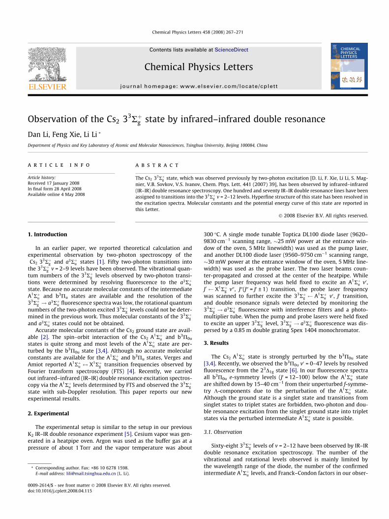
Hyperfine structure of the rotational lines has been resolved.Fig. 1 shows the excitation spectra of the 33Rþg v ¼ 4, N ¼159 A1Rþu v0 ¼ 9, J0 = 160 and 33Rþg v ¼ 5, N ¼ 102 A1Rþu v0 ¼10, J0 = 101 lines. The fine–hyperfine components of a N J0 rota-tional line spread about 10 GHz. Line shapes of other excitation
-6 -4 -2 0 2 4 6
4
6
8
10
GHz
Rel
ativ
e In
tens
ity
19811.860 cm-1
-6 -4 -2 0 2 4 6
4
6
8
10
12
GHz
19710.995 cm-1
Rel
ativ
e In
tens
ity
a
b
Fig. 1. Hyperfine splitting of the excitation lines: (a) 33Rþg v ¼ 4, N ¼ 159 A1Rþuv0 = 9, J0 = 160 transition and (b) 33Rþg v ¼ 5, N ¼ 102 A1Rþu v0 = 10, J0 = 101transition.
transitions are similar and we take the positions of the center ofgravity of the excitation lines as the probe frequencies to calculatethe term values of the rotational levels. The excitation data aregiven in Table A1 of Appendix A.
The 33Rþg ! a3Rþu fluorescence pattern from a given 33Rþg v levelexcited by IR–IR double resonance excitation is the same as thepattern from the same vibrational level excited by two-photonexcitation [1]. The vibrational quantum numbers are thus deter-mined by resolved fluorescence to the a3Rþu state as described inthe two-photon spectroscopy. In our previous Li2, Na2, and K2
experiments, double resonance signals were normally much stron-ger than two-photon excitation signals, and resolved fluorescencespectra from double resonance excited levels have much better sig-nal/noise ratio. In this Cs2 33Rþg state case, however, the resolvedfluorescence spectra recorded from two-photon excited 33Rþg lev-els have better S/N. Our previous Cs2 two-photon excitation wasDoppler-limited. The Cs2 molecules absorbed two photons withsame propagating direction and no fine–hyperfine structure wasresolved. The current double resonance excitation, however, hassub-Doppler resolution and hyperfine structure has been resolved.The hyperfine components of a rotational line spread �10 GHz.Although the total intensity (the sum of all components) is stron-ger than the two-photon signal, the fluorescence spectra could berecorded only when the probe laser was held fixed to one compo-nent, and thus the S/N is not as good as in Ref. [1].
The rotational constant of the a3Rþu state is very small(�0.006 cm�1) [1]. Our S/N ratio of the 33Rþg ! a3Rþu fluorescencespectra could not provide more information for the a3Rþu state.High-resolution fluorescence spectroscopy, FTS for example, willbe more powerful to solve this problem.
3.2. Molecular constants and potential energy curve
Table 1 gives the molecular constants by a standard Dunham fit.Using these molecular constants, the Rydberg–Klein–Rees (RKR)potential curve has been constructed (Table 2). We also performeda direct-potential-fit (DPF) [7] from the observed term values andobtained the expanded Morse oscillator (EMO) potential curve (Ta-ble 3, the vibrational energies and rotational constants calculatedfrom this potential curve are also listed in Table 2). The RKR andEMO potential curves can reproduce the observed energy levelsas well as the Dunham constants. Fig. 2 (from Table A2 of AppendixA) shows the deviations between the observed term values and thecalculated values from the Dunham constants, the RKR potentialcurve, and the EMO curve. The EMO potential curve reproducesthe energy levels better than the RKR curve. The 33Rþg v = 2,N = 41 and v = 11, N = 173 levels have bigger deviations (Fig. 2and Table A2 of Appendix A), which could be due to perturbations.
Table 1Molecular constants of the Cs2 33Rþg state
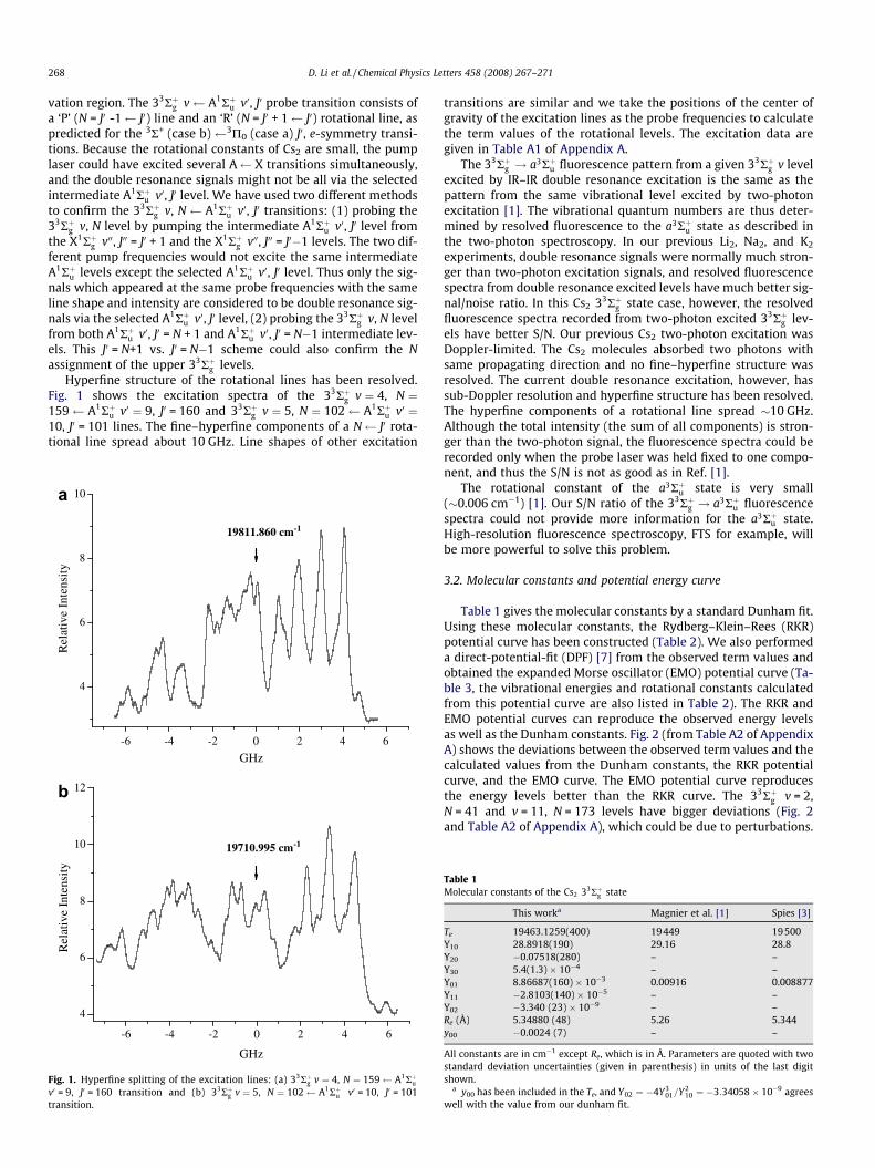
This worka Magnier et al. [1] Spies [3]
Te 19463.1259(400) 19449 19500Y10 28.8918(190) 29.16 28.8Y20 �0.07518(280) – –Y30 5.4(1.3) � 10�4 – –Y01 8.86687(160) � 10�3 0.00916 0.008877Y11 �2.8103(140) � 10�5 – –Y02 �3.340 (23) � 10�9 – –Re (Å) 5.34880 (48) 5.26 5.344y00 �0.0024 (7) – –
All constants are in cm�1 except Re, which is in Å. Parameters are quoted with twostandard deviation uncertainties (given in parenthesis) in units of the last digitshown.
a y00 has been included in the Te, and Y02 ¼ �4Y301=Y2
10 ¼ �3:34058� 10�9 agreeswell with the value from our dunham fit.
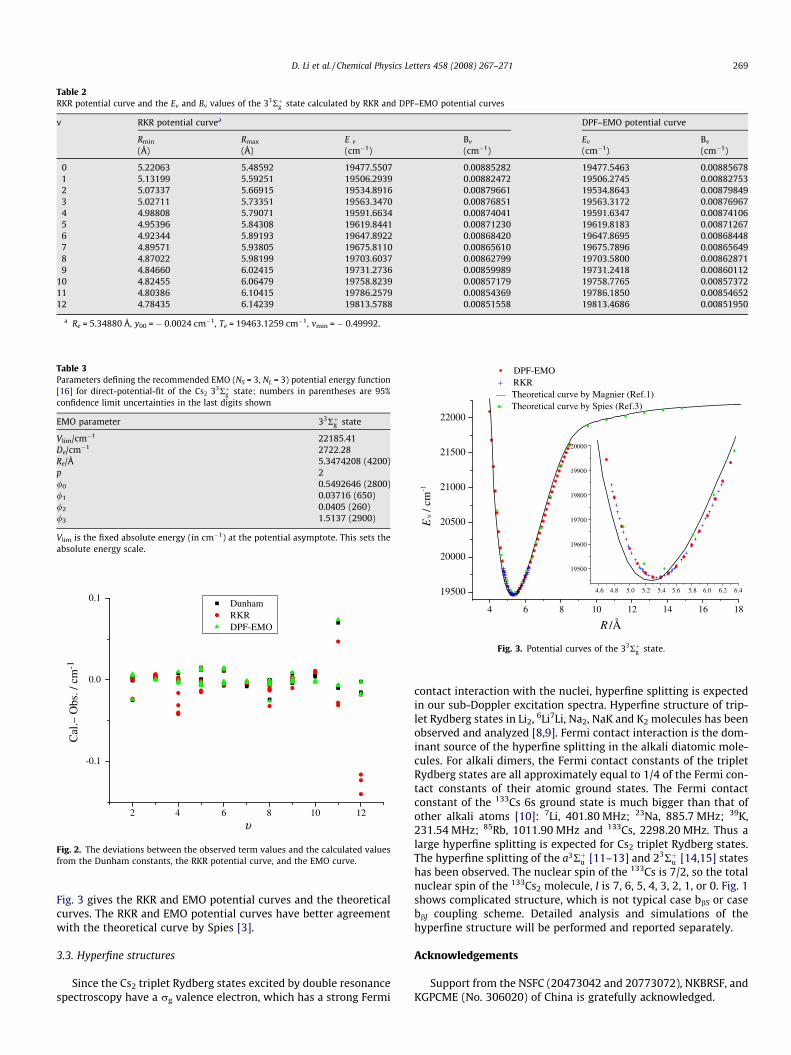
Table 2RKR potential curve and the Ev and Bv values of the 33Rþg state calculated by RKR and DPF–EMO potential curves
v RKR potential curvea DPF–EMO potential curve
Rmin
(Å)Rmax
(Å)E v
(cm�1)Bv
(cm�1)Ev
(cm�1)Bv
(cm�1)
0 5.22063 5.48592 19477.5507 0.00885282 19477.5463 0.008856781 5.13199 5.59251 19506.2939 0.00882472 19506.2745 0.008827532 5.07337 5.66915 19534.8916 0.00879661 19534.8643 0.008798493 5.02711 5.73351 19563.3470 0.00876851 19563.3172 0.008769674 4.98808 5.79071 19591.6634 0.00874041 19591.6347 0.008741065 4.95396 5.84308 19619.8441 0.00871230 19619.8183 0.008712676 4.92344 5.89193 19647.8922 0.00868420 19647.8695 0.008684487 4.89571 5.93805 19675.8110 0.00865610 19675.7896 0.008656498 4.87022 5.98199 19703.6037 0.00862799 19703.5800 0.008628719 4.84660 6.02415 19731.2736 0.00859989 19731.2418 0.00860112
10 4.82455 6.06479 19758.8239 0.00857179 19758.7765 0.0085737211 4.80386 6.10415 19786.2579 0.00854369 19786.1850 0.0085465212 4.78435 6.14239 19813.5788 0.00851558 19813.4686 0.00851950
a Re = 5.34880 Å, y00 = � 0.0024 cm�1, Te = 19463.1259 cm�1, vmin = � 0.49992.
Table 3Parameters defining the recommended EMO (NS = 3, NL = 3) potential energy function[16] for direct-potential-fit of the Cs2 33Rþg state; numbers in parentheses are 95%confidence limit uncertainties in the last digits shown
EMO parameter 33Rþg state
Vlim/cm�1 22185.41De/cm�1 2722.28Re/Å 5.3474208 (4200)p 2/0 0.5492646 (2800)/1 0.03716 (650)/2 0.0405 (260)/3 1.5137 (2900)
Vlim is the fixed absolute energy (in cm�1) at the potential asymptote. This sets theabsolute energy scale.
2 4 6 8 10 12
-0.1
0.0
0.1
Cal
.− O
bs. /
cm
-1
υ
Dunham RKR DPF-EMO
Fig. 2. The deviations between the observed term values and the calculated valuesfrom the Dunham constants, the RKR potential curve, and the EMO curve.
4 6 8 10 12 14 16 18
19500
20000
20500
21000
21500
22000
4.6 4.8 5.0 5.2 5.4 5.6 5.8 6.0 6.2 6.4
19500
19600
19700
19800
19900
20000
Eυ /
cm
-1
R /Å
DPF-EMO+ RKR
⎯ Theoretical curve by Magnier (Ref.1)• Theoretical curve by Spies (Ref.3)
Fig. 3. Potential curves of the 33Rþg state.
D. Li et al. / Chemical Physics Letters 458 (2008) 267–271 269
Fig. 3 gives the RKR and EMO potential curves and the theoreticalcurves. The RKR and EMO potential curves have better agreementwith the theoretical curve by Spies [3].
3.3. Hyperfine structures
Since the Cs2 triplet Rydberg states excited by double resonancespectroscopy have a rg valence electron, which has a strong Fermi
contact interaction with the nuclei, hyperfine splitting is expectedin our sub-Doppler excitation spectra. Hyperfine structure of trip-let Rydberg states in Li2, 6Li7Li, Na2, NaK and K2 molecules has beenobserved and analyzed [8,9]. Fermi contact interaction is the dom-inant source of the hyperfine splitting in the alkali diatomic mole-cules. For alkali dimers, the Fermi contact constants of the tripletRydberg states are all approximately equal to 1/4 of the Fermi con-tact constants of their atomic ground states. The Fermi contactconstant of the 133Cs 6s ground state is much bigger than that ofother alkali atoms [10]: 7Li, 401.80 MHz; 23Na, 885.7 MHz; 39K,231.54 MHz; 85Rb, 1011.90 MHz and 133Cs, 2298.20 MHz. Thus alarge hyperfine splitting is expected for Cs2 triplet Rydberg states.The hyperfine splitting of the a3Rþu [11–13] and 23Rþu [14,15] stateshas been observed. The nuclear spin of the 133Cs is 7/2, so the totalnuclear spin of the 133Cs2 molecule, I is 7, 6, 5, 4, 3, 2, 1, or 0. Fig. 1shows complicated structure, which is not typical case bbS or casebbJ coupling scheme. Detailed analysis and simulations of thehyperfine structure will be performed and reported separately.
Acknowledgements
Support from the NSFC (20473042 and 20773072), NKBRSF, andKGPCME (No. 306020) of China is gratefully acknowledged.

Table A1 (continued)
IntermediateA level
Probelaser frequency�1
33Rþg state
270 D. Li et al. / Chemical Physics Letters 458 (2008) 267–271
Appendix A
See Tables A1 and A2.
Table A1Supplemental IR–IR excitation data: intermediate levels, probe laser frequencies, thev, N assignment and term values of the 33Rþg state
IntermediateA level
Probelaser frequencycm�1
33Rþg state
v0 J0 Term value(cm�1)
v N
6 42 9659.130 19550.054 2 416 42 9659.130 19550.054 2 416 42 9660.595 19551.519 2 436 42 9660.595 19551.519 2 436 44 9658.998 19551.519 2 436 44 9658.998 19551.519 2 436 44 9660.562 19553.083 2 456 44 9660.562 19553.083 2 456 46 9658.890 19553.082 2 456 46 9658.890 19553.082 2 456 46 9660.524 19554.716 2 476 46 9660.524 19554.716 2 474 70 9735.803 19577.302 2 694 70 9735.803 19577.302 2 694 70 9738.274 19579.773 2 714 70 9738.274 19579.773 2 717 24 9648.684 19568.182 3 237 24 9649.542 19569.040 3 257 24 9649.543 19569.041 3 256 42 9687.510 19578.434 3 416 42 9687.510 19578.434 3 416 42 9688.999 19579.923 3 436 42 9688.998 19579.922 3 436 44 9687.402 19579.923 3 436 44 9687.402 19579.923 3 436 44 9688.960 19581.481 3 456 44 9688.960 19581.481 3 456 46 9687.289 19581.481 3 456 46 9688.917 19583.109 3 476 46 9688.917 19583.109 3 477 24 9676.989 19596.487 4 237 24 9676.990 19596.488 4 237 24 9677.845 19597.343 4 257 24 9677.845 19597.343 4 256 42 9715.782 19606.706 4 416 42 9715.781 19606.705 4 416 42 9717.266 19608.190 4 436 42 9717.265 19608.189 4 436 44 9715.668 19608.189 4 436 44 9717.222 19609.743 4 456 44 9717.222 19609.743 4 456 46 9715.550 19609.742 4 456 46 9717.173 19611.365 4 476 46 9717.174 19611.366 4 478 78 9633.377 19644.039 4 778 78 9633.378 19644.040 4 778 78 9636.108 19646.770 4 798 78 9636.109 19646.771 4 799 160 9581.050 19811.860 4 1599 160 9581.051 19811.861 4 1599 160 9586.550 19817.360 4 1619 160 9586.550 19817.360 4 1619 222 9565.440 20012.448 4 2219 222 9565.440 20012.448 4 2219 222 9572.925 20019.933 4 2239 222 9572.925 20019.933 4 2239 224 9564.818 20019.933 4 2239 224 9572.329 20027.444 4 2259 226 9564.192 20027.480 4 2259 226 9564.192 20027.480 4 2259 226 9571.789 20035.077 4 2279 226 9571.789 20035.077 4 2278 78 9661.391 19672.053 5 778 78 9661.393 19672.055 5 77
cmv0 J0 Term value
(cm�1)v N
8 78 9664.114 19674.776 5 798 78 9664.114 19674.776 5 79
10 99 9578.687 19704.043 5 9810 99 9578.687 19704.043 5 9810 100 9578.486 19705.773 5 9910 100 9578.486 19705.773 5 9910 99 9582.127 19707.483 5 10010 99 9582.127 19707.483 5 10010 101 9578.270 19707.484 5 10010 101 9578.271 19707.485 5 10010 100 9581.961 19709.248 5 10110 100 9581.961 19709.248 5 10110 102 9578.104 19709.247 5 10110 102 9578.104 19709.247 5 10110 101 9581.781 19710.995 5 10210 101 9581.780 19710.994 5 10210 102 9581.648 19712.791 5 10310 102 9581.647 19712.790 5 103
9 160 9608.512 19839.322 5 1599 160 9608.512 19839.322 5 1599 160 9613.996 19844.806 5 1619 160 9613.996 19844.806 5 161
10 99 9606.463 19731.819 6 9810 99 9606.464 19731.820 6 9810 100 9606.258 19733.545 6 9910 100 9606.258 19733.545 6 9910 99 9609.895 19735.251 6 10010 99 9609.895 19735.251 6 10010 101 9606.036 19735.250 6 10010 101 9606.036 19735.250 6 10010 100 9609.722 19737.009 6 10110 100 9609.721 19737.008 6 10110 102 9605.863 19737.006 6 10110 102 9605.865 19737.008 6 10110 101 9609.533 19738.747 6 10210 101 9609.534 19738.748 6 10210 102 9609.395 19740.538 6 10310 102 9609.395 19740.538 6 103
8 78 9717.023 19727.685 7 778 78 9717.024 19727.686 7 778 78 9719.730 19730.392 7 798 78 9719.730 19730.392 7 798 80 9716.803 19730.391 7 798 80 9716.804 19730.392 7 798 80 9719.577 19733.165 7 818 80 9719.576 19733.164 7 81
10 100 9661.411 19788.698 8 9910 100 9661.411 19788.698 8 9910 100 9664.854 19792.141 8 10110 100 9664.854 19792.141 8 10110 102 9660.997 19792.140 8 10110 102 9660.997 19792.140 8 10110 102 9664.506 19795.649 8 10310 102 9664.506 19795.649 8 103
9 160 9690.128 19920.938 8 1599 160 9690.130 19920.940 8 1599 160 9695.581 19926.391 8 1619 160 9695.581 19926.391 8 161
11 170 9606.192 19948.730 8 16911 170 9606.192 19948.730 8 16911 172 9605.649 19954.483 8 17111 172 9605.649 19954.483 8 17111 172 9611.463 19960.297 8 17311 172 9611.463 19960.297 8 17310 100 9688.801 19816.088 9 9910 100 9688.801 19816.088 9 9910 100 9692.230 19819.517 9 10110 100 9692.229 19819.516 9 10110 102 9688.374 19819.517 9 10110 102 9688.374 19819.517 9 10110 102 9691.870 19823.013 9 10310 102 9691.870 19823.013 9 103
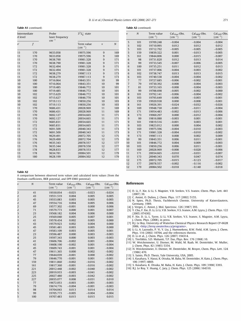
Table A1 (continued)
IntermediateA level
Probelaser frequencycm�1
33Rþg state
v0 J0 Term value(cm�1)
v N
11 170 9633.058 19975.596 9 16911 170 9633.058 19975.596 9 16911 170 9638.790 19981.328 9 17111 170 9638.790 19981.328 9 17111 172 9632.494 19981.328 9 17111 172 9632.494 19981.328 9 17111 172 9638.279 19987.113 9 17311 172 9638.279 19987.113 9 17310 100 9716.064 19843.351 10 9910 100 9716.064 19843.351 10 9910 100 9719.485 19846.772 10 10110 100 9719.485 19846.772 10 10110 102 9715.629 19846.772 10 10110 102 9715.627 19846.770 10 10110 102 9719.113 19850.256 10 10310 102 9719.113 19850.256 10 10311 170 9686.431 20028.969 11 16911 170 9686.431 20028.969 11 16911 170 9692.127 20034.665 11 17111 170 9692.127 20034.665 11 17111 172 9685.831 20034.665 11 17111 172 9685.831 20034.665 11 17111 172 9691.509 20040.343 11 17311 172 9691.509 20040.343 11 17313 176 9629.491 20072.705 12 17513 176 9629.490 20072.704 12 17513 176 9635.343 20078.557 12 17713 176 9635.344 20078.558 12 17713 178 9628.833 20078.553 12 17713 178 9634.781 20084.501 12 17913 180 9628.199 20084.502 12 179
Table A2A comparison between observed term values and calculated term values (from theDunham coefficients, RKR potential, and DPF-EMO potential)
v N Term value(cm�1)
Cal.Dun-Obs.(cm�1)
Cal.RKR-Obs.(cm�1)
Cal.DPF-Obs.(cm�1)
2 41 19550.054 �0.025 �0.023 �0.0242 43 19551.519 0.004 0.005 0.0052 45 19553.083 0.003 0.005 0.0052 47 19554.716 0.004 0.005 0.0062 69 19577.302 �0.001 0.000 0.0062 71 19579.773 0.000 0.001 0.0073 23 19568.182 0.004 0.006 0.0003 25 19569.040 0.005 0.007 0.0013 41 19578.434 0.002 0.005 0.0003 43 19579.923 0.002 0.004 0.0003 45 19581.481 0.003 0.005 0.0003 47 19583.109 0.003 0.005 0.0014 23 19596.487 0.000 0.003 �0.0034 25 19597.343 0.000 0.003 �0.0034 41 19606.706 �0.002 0.001 �0.0044 43 19608.190 �0.002 0.001 �0.0044 45 19609.743 �0.001 0.001 �0.0044 47 19611.365 0.000 0.002 �0.0024 77 19644.039 �0.001 0.000 �0.0024 79 19646.770 �0.001 0.001 �0.0014 159 19811.860 �0.002 �0.016 �0.0024 161 19817.360 �0.001 �0.016 �0.0024 221 20012.448 �0.002 �0.040 �0.0024 223 20019.933 �0.003 �0.041 �0.0024 225 20027.480 �0.003 �0.042 �0.0024 227 20035.077 0.008 �0.031 0.0105 77 19672.053 �0.003 �0.001 �0.0035 79 19674.776 �0.004 �0.001 �0.0035 98 19704.043 0.013 0.014 0.0145 99 19705.773 �0.005 �0.004 �0.0045 100 19707.483 0.015 0.015 0.015
Table A2 (continued)
v N Term value(cm�1)
Cal.Dun-Obs.(cm�1)
Cal.RKR-Obs.(cm�1)
Cal.DPF-Obs.(cm�1)
5 101 19709.248 �0.004 �0.004 �0.0045 102 19710.995 0.012 0.012 0.0125 103 19712.792 �0.005 �0.005 �0.0055 159 19839.322 0.001 �0.013 �0.0055 161 19844.806 0.000 �0.015 �0.0076 98 19731.820 0.012 0.013 0.0146 99 19733.545 �0.007 �0.006 �0.0056 100 19735.251 0.011 0.012 0.0136 101 19737.006 �0.004 �0.003 �0.0026 102 19738.747 0.013 0.013 0.0156 103 19740.538 �0.004 �0.004 �0.0027 77 19727.685 �0.006 �0.002 �0.0017 79 19730.392 �0.008 �0.004 �0.0037 81 19733.165 �0.008 �0.004 �0.0038 99 19788.698 �0.005 �0.002 0.0008 101 19792.141 �0.006 �0.004 �0.0028 103 19795.649 �0.006 �0.003 �0.0018 159 19920.938 0.000 �0.008 �0.0018 161 19926.391 �0.024 �0.032 �0.0268 169 19948.730 �0.001 �0.011 �0.0048 171 19954.483 �0.002 �0.013 �0.0068 173 19960.297 0.000 �0.012 �0.0049 99 19816.088 �0.003 0.001 �0.0019 101 19819.516 �0.001 0.003 0.0019 103 19823.012 0.000 0.004 0.0029 169 19975.596 �0.004 �0.010 �0.0039 171 19981.328 �0.004 �0.010 �0.0029 173 19987.113 0.008 0.002 0.009
10 99 19843.351 0.006 0.011 �0.00110 101 19846.772 0.004 0.009 �0.00310 103 19850.256 0.006 0.011 �0.00111 169 20028.969 �0.008 �0.028 �0.00611 171 20034.665 �0.010 �0.031 �0.00711 173 20040.343 0.070 0.047 0.07412 175 20072.705 �0.015 �0.123 �0.01712 177 20078.557 �0.002 �0.116 �0.00212 179 20084.502 �0.018 �0.140 �0.018
D. Li et al. / Chemical Physics Letters 458 (2008) 267–271 271
References
[1] D. Li, F. Xie, Li Li, S. Magnier, V.B. Sovkov, V.S. Ivanov, Chem. Phys. Lett. 441(2007) 39.
[2] C. Amiot, O. Dulieu, J. Chem. Phys. 117 (2002) 5155.[3] N. Spies, Ph.D. Thesis, Fachbereich Chemie, University of Kaiserslautern,
Germany, 1989.[4] J. Verges, C. Amiot, J. Mol. Spectrosc. 126 (1987) 393.[5] Y. Chu, F. Xie, D. Li, Li Li, V.B. Sovkov, V.S. Ivanov, A.M. Lyyra, J. Chem. Phys. 122
(2005) 074302.[6] F. Xie, D. Li, L. Tyree, Li Li, V.B. Sovkov, V.S. Ivanov, S. Magnier, A.M. Lyyra,
J. Chem. Phys. (2008), in press.[7] R.J. Le Roy, University of Waterloo Chemical Physics Research Report CP-662R
2006, <http://leroy.uwaterloo.ca/programs>.[8] Li Li, A. Lazoudis, P. Yi, Y. Liu, J. Huennekens, R.W. Field, A.M. Lyyra, J. Chem.
Phys. 116 (2002) 10704, and the references therein.[9] D. Li et al., J. Chem. Phys. 126 (2007) 194314.
[10] L. Tterlikkis, S.D. Mahanti, T.P. Das, Phys. Rev. 176 (1968) 10.[11] W. Weickenmeier, U. Diemer, M. Wahl, M. Raab, W. Demtröder, W. Muller,
J. Chem. Phys. 82 (1985) 5354.[12] H. Weickenmeier, U. Diemer, W. Demtröder, M. Broyer, Chem. Phys. Lett. 124
(1986) 470.[13] S. Sainis, Ph.D. Thesis, Yale University, USA, 2005.[14] S. Kasahara, Y. Hasui, K. Otsuka, M. Baba, W. Demtröder, H. Kato, J. Chem. Phys.
106 (1997) 4869.[15] S. Kasahara, K. Otsuka, M. Baba, H. Kato, J. Chem. Phys. 109 (1998) 3393.[16] R.J. Le Roy, Y. Huang, C. Jary, J. Chem. Phys. 125 (2006) 164310.