OBS-3+ and OBS300 Suspended Solids and Turbidity ….pdf · Limited Warranty “Products manufactured by CSI are warranted by CSI to be free from defects in materials and workmanship

INST

RU

CT

ION

MA

NU

AL

OBS-3+ and OBS300 Suspended Solids and

Turbidity Monitors Revision: 4/17

C o p y r i g h t © 2 0 0 8 - 2 0 1 7 C a m p b e l l S c i e n t i f i c , I n c .

Limited Warranty “Products manufactured by CSI are warranted by CSI to be free from defects in materials and workmanship under normal use and service for twelve months from the date of shipment unless otherwise specified in the corresponding product manual. (Product manuals are available for review online at www.campbellsci.com.) Products not manufactured by CSI, but that are resold by CSI, are warranted only to the limits extended by the original manufacturer. Batteries, fine-wire thermocouples, desiccant, and other consumables have no warranty. CSI’s obligation under this warranty is limited to repairing or replacing (at CSI’s option) defective Products, which shall be the sole and exclusive remedy under this warranty. The Customer assumes all costs of removing, reinstalling, and shipping defective Products to CSI. CSI will return such Products by surface carrier prepaid within the continental United States of America. To all other locations, CSI will return such Products best way CIP (port of entry) per Incoterms ® 2010. This warranty shall not apply to any Products which have been subjected to modification, misuse, neglect, improper service, accidents of nature, or shipping damage. This warranty is in lieu of all other warranties, expressed or implied. The warranty for installation services performed by CSI such as programming to customer specifications, electrical connections to Products manufactured by CSI, and Product specific training, is part of CSI's product warranty. CSI EXPRESSLY DISCLAIMS AND EXCLUDES ANY IMPLIED WARRANTIES OF MERCHANTABILITY OR FITNESS FOR A PARTICULAR PURPOSE. CSI hereby disclaims, to the fullest extent allowed by applicable law, any and all warranties and conditions with respect to the Products, whether express, implied or statutory, other than those expressly provided herein.”

http://www.campbellsci.com/

Assistance Products may not be returned without prior authorization. The following contact information is for US and international customers residing in countries served by Campbell Scientific, Inc. directly. Affiliate companies handle repairs for customers within their territories. Please visit www.campbellsci.com to determine which Campbell Scientific company serves your country.

To obtain a Returned Materials Authorization (RMA) number, contact CAMPBELL SCIENTIFIC, INC., phone (435) 227-9000. Please write the issued RMA number clearly on the outside of the shipping container. Campbell Scientific’s shipping address is:

CAMPBELL SCIENTIFIC, INC. RMA#_____ 815 West 1800 North Logan, Utah 84321-1784

For all returns, the customer must fill out a “Statement of Product Cleanliness and Decontamination” form and comply with the requirements specified in it. The form is available from our website at www.campbellsci.com/repair. A completed form must be either emailed to [email protected] or faxed to (435) 227-9106. Campbell Scientific is unable to process any returns until we receive this form. If the form is not received within three days of product receipt or is incomplete, the product will be returned to the customer at the customer’s expense. Campbell Scientific reserves the right to refuse service on products that were exposed to contaminants that may cause health or safety concerns for our employees.

Safety DANGER — MANY HAZARDS ARE ASSOCIATED WITH INSTALLING, USING, MAINTAINING, AND WORKING ON OR AROUND TRIPODS, TOWERS, AND ANY ATTACHMENTS TO TRIPODS AND TOWERS SUCH AS SENSORS, CROSSARMS, ENCLOSURES, ANTENNAS, ETC. FAILURE TO PROPERLY AND COMPLETELY ASSEMBLE, INSTALL, OPERATE, USE, AND MAINTAIN TRIPODS, TOWERS, AND ATTACHMENTS, AND FAILURE TO HEED WARNINGS, INCREASES THE RISK OF DEATH, ACCIDENT, SERIOUS INJURY, PROPERTY DAMAGE, AND PRODUCT FAILURE. TAKE ALL REASONABLE PRECAUTIONS TO AVOID THESE HAZARDS. CHECK WITH YOUR ORGANIZATION'S SAFETY COORDINATOR (OR POLICY) FOR PROCEDURES AND REQUIRED PROTECTIVE EQUIPMENT PRIOR TO PERFORMING ANY WORK.

Use tripods, towers, and attachments to tripods and towers only for purposes for which they are designed. Do not exceed design limits. Be familiar and comply with all instructions provided in product manuals. Manuals are available at www.campbellsci.com or by telephoning (435) 227-9000 (USA). You are responsible for conformance with governing codes and regulations, including safety regulations, and the integrity and location of structures or land to which towers, tripods, and any attachments are attached. Installation sites should be evaluated and approved by a qualified engineer. If questions or concerns arise regarding installation, use, or maintenance of tripods, towers, attachments, or electrical connections, consult with a licensed and qualified engineer or electrician.

General • Prior to performing site or installation work, obtain required approvals and permits. Comply

with all governing structure-height regulations, such as those of the FAA in the USA. • Use only qualified personnel for installation, use, and maintenance of tripods and towers, and

any attachments to tripods and towers. The use of licensed and qualified contractors is highly recommended.

• Read all applicable instructions carefully and understand procedures thoroughly before beginning work.

• Wear a hardhat and eye protection, and take other appropriate safety precautions while working on or around tripods and towers.

• Do not climb tripods or towers at any time, and prohibit climbing by other persons. Take reasonable precautions to secure tripod and tower sites from trespassers.

• Use only manufacturer recommended parts, materials, and tools.

Utility and Electrical • You can be killed or sustain serious bodily injury if the tripod, tower, or attachments you are

installing, constructing, using, or maintaining, or a tool, stake, or anchor, come in contact with overhead or underground utility lines.

• Maintain a distance of at least one-and-one-half times structure height, 20 feet, or the distance required by applicable law, whichever is greater, between overhead utility lines and the structure (tripod, tower, attachments, or tools).

• Prior to performing site or installation work, inform all utility companies and have all underground utilities marked.

• Comply with all electrical codes. Electrical equipment and related grounding devices should be installed by a licensed and qualified electrician.

Elevated Work and Weather • Exercise extreme caution when performing elevated work. • Use appropriate equipment and safety practices. • During installation and maintenance, keep tower and tripod sites clear of un-trained or non-

essential personnel. Take precautions to prevent elevated tools and objects from dropping. • Do not perform any work in inclement weather, including wind, rain, snow, lightning, etc.

Maintenance • Periodically (at least yearly) check for wear and damage, including corrosion, stress cracks,

frayed cables, loose cable clamps, cable tightness, etc. and take necessary corrective actions. • Periodically (at least yearly) check electrical ground connections.

WHILE EVERY ATTEMPT IS MADE TO EMBODY THE HIGHEST DEGREE OF SAFETY IN ALL CAMPBELL SCIENTIFIC PRODUCTS, THE CUSTOMER ASSUMES ALL RISK FROM ANY INJURY RESULTING FROM IMPROPER INSTALLATION, USE, OR MAINTENANCE OF TRIPODS, TOWERS, OR ATTACHMENTS TO TRIPODS AND TOWERS SUCH AS SENSORS, CROSSARMS, ENCLOSURES, ANTENNAS, ETC.

i

Table of Contents PDF viewers: These page numbers refer to the printed version of this document. Use the PDF reader bookmarks tab for links to specific sections.

1. Introduction ................................................................ 1

2. Precautions ................................................................ 1

3. Initial Inspection ......................................................... 2

4. QuickStart ................................................................... 2

4.1 Preparation for Use .............................................................................. 2 4.2 Use SCWin to Program Datalogger and Generate Wiring Diagram .... 2

5. Overview ..................................................................... 4

5.1 Applications ......................................................................................... 5 5.2 Turbidity .............................................................................................. 5 5.3 Design Details ...................................................................................... 5 5.4 Measurement Details ............................................................................ 6

6. Specifications ............................................................. 7

7. Installation .................................................................. 9

7.1 Pre-Deployment Tests .......................................................................... 9 7.2 Mounting Considerations ..................................................................... 9

7.2.1 Siting ............................................................................................. 9 7.2.2 Mounting Options ......................................................................... 9

7.2.2.1 PVC Pipe ............................................................................ 9 7.2.2.2 Cable Ties or Hose Clamps .............................................. 10

7.3 Wiring to Datalogger ......................................................................... 10 7.4 Datalogger Programming ................................................................... 11 7.5 Calibration Certificate ........................................................................ 12

8. Calibration ................................................................ 14

8.1 Turbidity ............................................................................................ 14 8.1.1 Materials and Equipment ............................................................ 16 8.1.2 Setup ........................................................................................... 17 8.1.3 Procedure .................................................................................... 17

8.2 Sediment ............................................................................................ 18 8.2.1 Dry-sediment Calibration ............................................................ 18 8.2.2 Wet-sediment Calibration ........................................................... 18 8.2.3 In situ Calibration ....................................................................... 19

8.2.3.1 Materials and Equipment .................................................. 19 8.2.3.2 Setup ................................................................................. 19 8.2.3.3 Procedure .......................................................................... 20

9. Troubleshooting ....................................................... 21

Table of Contents

ii

10. Maintenance ............................................................. 22

11. Factors that Affect Turbidity and Suspended-Sediment Measurements ....................................... 23

11.1 Particle Size ....................................................................................... 23 11.2 Suspensions with Mud and Sand ....................................................... 24 11.3 Particle-Shape Effects ....................................................................... 24 11.4 High Sediment Concentrations .......................................................... 25 11.5 IR Reflectivity—Sediment Color ...................................................... 26 11.6 Water Color ....................................................................................... 27 11.7 Bubbles and Plankton ........................................................................ 27 11.8 Biological and Chemical Fouling ...................................................... 28

12. References ................................................................ 28

13. Terminology ............................................................. 29

Appendices

A. Importing Short Cut Code Into CRBasic Editor ... A-1

B. Example Programs ................................................. B-1

B.1 CR1000 Example Program .............................................................. B-1 B.2 CR200(X) Example Program .......................................................... B-2

C. Electrical Connections Details .............................. C-1

D. Datalogger Connection to a Relay ........................ D-1

Figures 5-1. Components of the OBS-3+ (left) and orientation source beam

and detector acceptance cone of the OBS-3+ (top right) and OBS300 (bottom right) .................................................................... 6

7-1. OBS-3+ connected to a CR1000 Datalogger (OBS300 has the same wiring) .................................................................................. 11

7-2. Calibration certificate showing millivolt coefficients ....................... 13 7-3. Calibration certificate showing volts coefficients ............................. 14 8-1. Normalized response of OBS-3+ to AMCO Clear® turbidity. The

inset shows the response function of an OBS sensor to high sediment concentrations. ................................................................ 15

8-2. Position of OBS-3+ (left) and OBS300 (right) in clean tap water in big black tub .............................................................................. 17

8-3. OBS-3+ (left) and OBS300 (right) in 500-NTU AMCO Clear® turbidity standard in 100-mm black polyethylene calibration cup.................................................................................................. 18

8-4. Portable sediment suspender (left) and OBS beam orientation in suspender tub (right) ...................................................................... 20

11-1. Normalized OBS sensitivity as a function of grain diameter ............ 23

Table of Contents

iii

11-2. The apparent change in turbidity resulting from disaggregation methods........................................................................................... 24

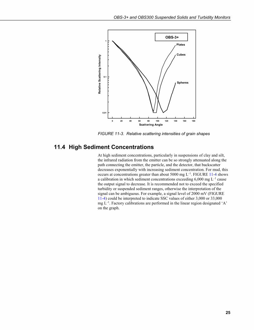
11-3. Relative scattering intensities of grain shapes .................................... 25 11-4. Response of an OBS sensor to a wide range of SSC .......................... 26 11-5. Infrared reflectivity of minerals as a function of 10-Munzell

value ............................................................................................... 27 C-1. Pin assignments for MCBH and MCIL wet-pluggable

connectors ..................................................................................... C-1 D-1. Wiring diagram for connecting an OBS sensor to an external

relay and a datalogger .................................................................. D-1

Tables 7-1. Wire Color, Function, and Datalogger Connection ............................ 10 8-1. SDVB NTU values for turbidity calibrations in standard low

ranges. ............................................................................................. 15 8-2. Change in NTU value resulting from one hour of evaporation1 of

SDVB standard; in other words, loss of water but not particles. .... 16 9-1. Troubleshooting Chart ....................................................................... 22 C-1. Pin numbers, electrical functions and wire color codes for OBS

sensor bulkhead connectors. ......................................................... C-2

CRBasic Examples B-1. CR1000 Program Measuring the Turbidity Sensor .......................... B-1 B-2. CR200X Program Measuring the Turbidity Sensor ......................... B-2

Table of Contents

iv

1

OBS-3+ and OBS300 Suspended Solids and Turbidity Monitors 1. Introduction

The OBS-3+ and OBS300 are submersible, turbidity sensors that use OBS® technology to measure suspended solids and turbidity for applications ranging from water quality in freshwater rivers and streams to sediment transport and dredge monitoring. The OBS-3+ and OBS300 are identical except for the orientation of their optics. The OBS-3+ “looks” perpendicular to the length of the sensor, whereas the OBS300 “looks” out the end of the sensor. Throughout this manual any time OBS sensor is mentioned, it is valid for both the OBS-3+ and OBS300.

This manual provides information only for CRBasic dataloggers. It is also compatible with most of our retired Edlog dataloggers. For Edlog datalogger support, see an older manual at www.campbellsci.com/old-manuals.

2. Precautions • READ AND UNDERSTAND the Safety section at the front of this

manual.

• Although the OBS-3+ and OBS300 are rugged, they should be handled as precision scientific instruments.

• The titanium body option (option -TB) must be used if submersing the probe in seawater. Using an OBS sensor with a stainless steel housing (option -SB) in seawater voids the warranty and causes corrosion and leakage.

• There are no user-serviceable parts inside the sensor housing. Do not remove the sensor or connector from the pressure housing. This will void the warranty and could cause leakage.

• Do not use solvents such as MEK, toluene, acetone, or trichloroethylene to clean the sensor.

• The sensor may be damaged if it is encased in ice.

• Damages caused by freezing conditions will not be covered by our warranty.

• Campbell Scientific recommends removing the sensor from the water for the time period that the water is likely to freeze.

NOTE

http://www.campbellsci.com/old-manuals

OBS-3+ and OBS300 Suspended Solids and Turbidity Monitors

2

3. Initial Inspection • Upon receipt of the OBS-3+ or OBS300, inspect the packaging and

contents for damage. File damage claims with the shipping company.

• The sensor is shipped with a calibration sheet and an instruction manual or a ResourceDVD.

4. QuickStart 4.1 Preparation for Use

1. Bench test the sensor to ensure that it functions properly prior to making field installations (see Section 7.1, Pre-Deployment Tests (p. 9)).

2. Calibrate the sensor using suspended solids from the waters that will be monitored (see Section 8, Calibration (p. 14)).

3. Refer to Section 7.2, Mounting Considerations (p. 9), for siting and mounting options.

4.2 Use SCWin to Program Datalogger and Generate Wiring Diagram

Short Cut is an easy way to program your datalogger to measure the sensor and assign datalogger wiring terminals. Short Cut is available as a download on www.campbellsci.com and the ResourceDVD. It is included in installations of LoggerNet, PC200W, PC400, or RTDAQ.

The following procedure shows using Short Cut to program the OBS-3+/OBS300.

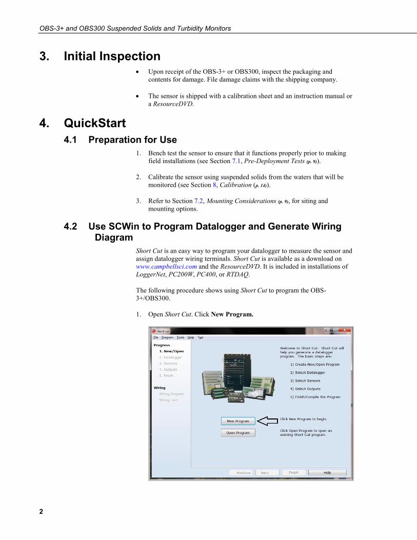
1. Open Short Cut. Click New Program.



3

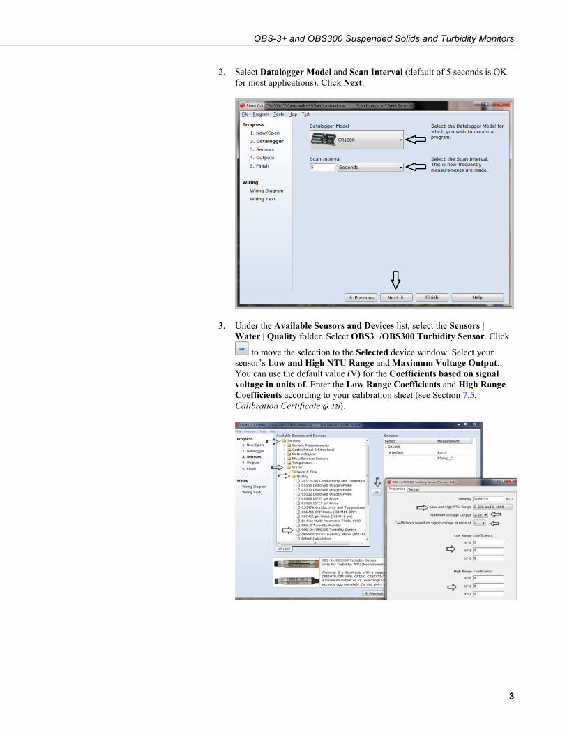
2. Select Datalogger Model and Scan Interval (default of 5 seconds is OK for most applications). Click Next.

3. Under the Available Sensors and Devices list, select the Sensors | Water | Quality folder. Select OBS3+/OBS300 Turbidity Sensor. Click

to move the selection to the Selected device window. Select your sensor’s Low and High NTU Range and Maximum Voltage Output. You can use the default value (V) for the Coefficients based on signal voltage in units of. Enter the Low Range Coefficients and High Range Coefficients according to your calibration sheet (see Section 7.5, Calibration Certificate (p. 12)).


4

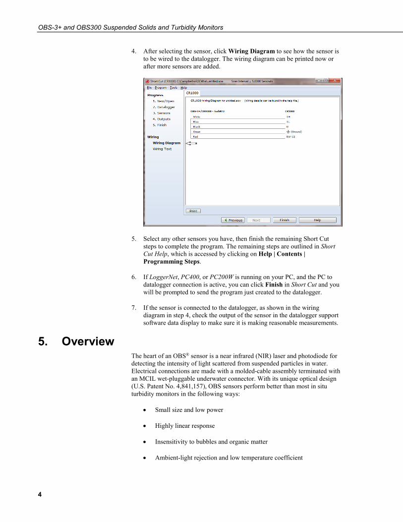
4. After selecting the sensor, click Wiring Diagram to see how the sensor is to be wired to the datalogger. The wiring diagram can be printed now or after more sensors are added.

5. Select any other sensors you have, then finish the remaining Short Cut steps to complete the program. The remaining steps are outlined in Short Cut Help, which is accessed by clicking on Help | Contents | Programming Steps.

6. If LoggerNet, PC400, or PC200W is running on your PC, and the PC to datalogger connection is active, you can click Finish in Short Cut and you will be prompted to send the program just created to the datalogger.

7. If the sensor is connected to the datalogger, as shown in the wiring diagram in step 4, check the output of the sensor in the datalogger support software data display to make sure it is making reasonable measurements.

5. Overview The heart of an OBS® sensor is a near infrared (NIR) laser and photodiode for detecting the intensity of light scattered from suspended particles in water. Electrical connections are made with a molded-cable assembly terminated with an MCIL wet-pluggable underwater connector. With its unique optical design (U.S. Patent No. 4,841,157), OBS sensors perform better than most in situ turbidity monitors in the following ways:

• Small size and low power

• Highly linear response

• Insensitivity to bubbles and organic matter

• Ambient-light rejection and low temperature coefficient


5

5.1 Applications OBS sensors are used for a wide variety of monitoring tasks in riverine, oceanic, laboratory, and industrial settings. They can be integrated in water-quality monitoring systems, CTDs, laboratory instrumentation, and sediment-transport monitors. The applications include:

• Compliance with permits, water-quality guidelines, and regulations

• Determination of transport and fate of particles and associated contaminants in aquatic systems

• Conservation, protection and restoration of surface waters

• Assess performance of water and land-use management

• Monitor waterside construction, mining, and dredging operations

• Characterization of wastewater and energy-production effluents

• Tracking water-well completion including development and use

5.2 Turbidity Conceptually, turbidity is a numerical expression in turbidity units (NTU) of the optical properties that cause water to appear hazy or cloudy as a result of light scattering and absorption by suspended matter. Operationally, a NTU value is interpolated from neighboring light-scattering measurements made on calibration standards such as Formazin, StablCal, or SDVB.

Turbidity is caused by suspended and dissolved matter such as sediment, plankton, bacteria, viruses, and organic and inorganic dyes. In general, as the concentration of suspended matter in water increases, so will its turbidity, and as the concentration of dissolved light-absorbing matter increases, turbidity will decrease. Descriptions of the factors that affect turbidity are given in Section 11, Factors that Affect Turbidity and Suspended-Sediment Measurements (p. 23).

Like all other optical turbidity monitors, the OBS response depends on the size, composition, and shape of suspended particles, and for this reason, the sensor must be calibrated with suspended solids from the waters to be monitored.

There is no ‘standard’ turbidimeter design or universal formula for converting NTU values to physical units such as mg L–1 or ppm. NTU values have no intrinsic physical, chemical, or biological significance. Empirical correlations between turbidity and environmental conditions, established through field calibration, can be useful in water-quality investigations.

5.3 Design Details OBS sensors detect suspended matter in water and turbidity from the relative intensity of light backscattered at angles ranging from 90o to 165o, in clean water. A 3D schematic of the main components of the OBS-3+ is shown in

CAUTION


6

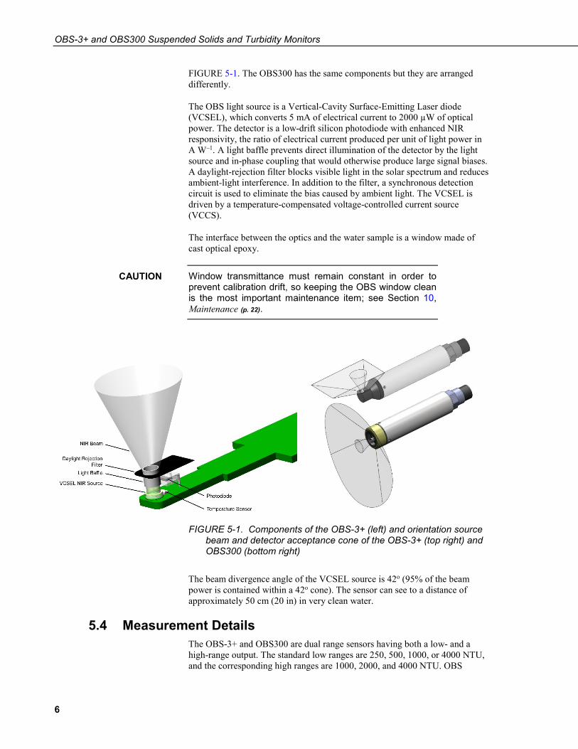
FIGURE 5-1. The OBS300 has the same components but they are arranged differently.

The OBS light source is a Vertical-Cavity Surface-Emitting Laser diode (VCSEL), which converts 5 mA of electrical current to 2000 µW of optical power. The detector is a low-drift silicon photodiode with enhanced NIR responsivity, the ratio of electrical current produced per unit of light power in A W–1. A light baffle prevents direct illumination of the detector by the light source and in-phase coupling that would otherwise produce large signal biases. A daylight-rejection filter blocks visible light in the solar spectrum and reduces ambient-light interference. In addition to the filter, a synchronous detection circuit is used to eliminate the bias caused by ambient light. The VCSEL is driven by a temperature-compensated voltage-controlled current source (VCCS).

The interface between the optics and the water sample is a window made of cast optical epoxy.

Window transmittance must remain constant in order to prevent calibration drift, so keeping the OBS window clean is the most important maintenance item; see Section 10, Maintenance (p. 22).

FIGURE 5-1. Components of the OBS-3+ (left) and orientation source beam and detector acceptance cone of the OBS-3+ (top right) and OBS300 (bottom right)

The beam divergence angle of the VCSEL source is 42o (95% of the beam power is contained within a 42o cone). The sensor can see to a distance of approximately 50 cm (20 in) in very clean water.

5.4 Measurement Details The OBS-3+ and OBS300 are dual range sensors having both a low- and a high-range output. The standard low ranges are 250, 500, 1000, or 4000 NTU, and the corresponding high ranges are 1000, 2000, and 4000 NTU. OBS

CAUTION


7

sensors can be purchased with a 4 to 20 mA current output on the low range and a 0 to 5 V output on the high range. Voltage outputs can be 0 to 2.5 or 0 to 5 V; see Section 6, Specifications (p. 7). It is also possible to purchase sensors configured to operate from 5-V power, however, the output span is limited to 2.5 V.

The sensor needs to be connected to a datalogger, current meter, or CTD instrument. The datalogger (or other device) powers the sensor, digitizes its analog signals, computes NTU and Suspended Solids Concentration (SSC) values, and records the statistical result in flash memory. To make the conversion from digitized signals to engineering units (for example, NTU, mg L–1, and ppm), the datalogger must have the calibration equations in its operating program or the conversion must be done in post processing.

When using some current meters or CTD instruments, the OBS sensor should be calibrated while it is connected to the device exactly as it will be used. The reason for this is that the factory calibration is performed with a NIST-traceable digital multimeter and the numerical values reported by some host devices not NIST-certified will be different.

6. Specifications Features:

• Measures suspended solids and turbidity for up to 4000 NTU • Provides a compact, low-power probe that is field proven • Stainless-steel body allows use down to 500 m in fresh water • Titanium body allows use down to 1500 m in fresh or salt water • Fitted with MCBH-5-FS, wet-pluggable connector—multiple mating

cable length options available • Accurate and rugged • Compatible with Campbell Scientific CRBasic dataloggers:

CR200(X) series, CR300 series, CR6 series, CR800 series, CR1000, CR3000, CR5000, and CR9000(X)

Operating Temperature: 0° to 40°C

Sensor may be damaged if it is encased in frozen liquid.

Ranges Turbidity (low/high): 250/1000 NTU; 500/2000 NTU; 1000/4000 NTU Mud1: 5000 to 10,000 mg L–1 Sand1: 50,000 to 100,000 mg L–1 1 Range depends on sediment size, particle shape, and reflectivity.

Accuracy Turbidity2: 2% of reading or 0.5 NTU Mud2: 2% of reading or 1 mg L–1 Sand2: 4% of reading or 10 mg L–1

2 Whichever is larger.

NOTE

CAUTION


8

Power Voltage output: 5 to 15 Vdc/15 mA (Volts outputs) 4-20 mA transmitter: 9 to 15 Vdc/45 mA max. (4 to 20 mA output)

Operating wave length: 850 ± 5 nm

Optical power: 2000 µW

Drift: <2% per year

Daylight rejection: –28 dB (re:48 mW cm–2)

Maximum data rate: 10 Hz

Minimum warm-up time: 2 s

Maximum depth Stainless steel body: 500 m (1640.5 ft) Titanium body: 1500 m (4921.5 ft)

Weight: 181.4 g (0.4 lb)

Dimensions: (see below)

131 mm (5.15 in)

25 mm (0.98 in)

141 mm (5.56 in)

25 mm (0.98 in)


9

7. Installation If you are programming your datalogger with Short Cut, skip Section 7.3, Wiring to Datalogger (p. 10), and Section 7.4, Datalogger Programming (p. 11). Short Cut does this work for you. See Section 4, QuickStart (p. 2), for a Short Cut tutorial.

7.1 Pre-Deployment Tests When the OBS sensor is received from the manufacturer, do the following bench test to ensure that it functions properly prior to field installations.

1. Connect the red and black wires in the cable supplied with the sensor to a 9 or 12 Vdc battery.

2. Plug the cable into the sensor and connect a multimeter across the blue (+ test lead) and green (– test lead) wires.

3. Wave your finger over the OBS sensor about 20 mm away from the window. The meter should indicate fluctuating signals ranging from a few mV or 4 mA to the span shown on the calibration certificate, 2.5 V, 5 V, or 20 mA (see Section 7.5, Calibration Certificate (p. 12)).

4. Switch the + DMM test lead to the white wire and repeat the test. The results should be similar.

7.2 Mounting Considerations Schemes for mounting the OBS-3+ and OBS300 will vary with applications; however, the same basic precautions should be followed to ensure the unit is able to make a good measurement and that it is not lost or damaged.

7.2.1 Siting The most important general precaution is to orient the unit so that the sensor looks into clear water without reflective surfaces. This includes any object such as a mounting structure, a streambed, or sidewalls. The sensor can see to a distance of about 50 cm (20 in) in very clean water at angles ranging from 125° to 170°. The OBS-3+ sensor point perpendicular to the sensor body whereas the OBS300 sensor is orientated to point out the end (see FIGURE 5-1).

The sensor has ambient-light rejection features, but it is still best to orient it away from the influence of direct sunlight. Shading may be required in some installations to totally protect from sunlight interference.

7.2.2 Mounting Options 7.2.2.1 PVC Pipe

Mounting the sensor inside the end of a PVC pipe is a convenient way to provide structure and protection for deployments. The OBS-3+/OBS300 will fit inside a 1.25-in. schedule 40 PVC pipe.


10

7.2.2.2 Cable Ties or Hose Clamps The OBS-3+/OBS300 can be mounted to a frame or post using large, high-strength nylon cable ties (7.6 mm (0.3 in) width) or stainless steel hose clamps. When using clamps, do the following:

1. Cover the area(s) to be clamped with tape or 2 mm (1/16 in) neoprene sheet.

2. Clamp the unit to the mounting frame or wire using the padded area. Spacer blocks may be necessary to prevent the unit from chafing with the frame or wire.

Do not tighten the hose clamps more than is necessary to produce a firm grip. Overtightening may damage the pressure housing causing leakage.

7.3 Wiring to Datalogger TABLE 7-1 and FIGURE 7-1 show the recommended wiring configuration for connecting the OBS sensor to a Campbell Scientific datalogger; wiring to dataloggers manufactured by other companies is similar. In this configuration, single-ended analog inputs are used to measure the OBS sensors’ voltage signal. The red power wire is connected to a switched 12 V channel, which allows the OBS sensor to be turned off when it is not making measurements. This reduces current consumption. Dataloggers that do not have a switched 12 V channel can use a relay to turn the OBS sensor off and on. Appendix D, Datalogger Connection to a Relay (p. D-1), provides information about using a relay.

TABLE 7-1. Wire Color, Function, and Datalogger Connection

Wire Color

Wire Function Datalogger Connection Terminal

White High Range Signal

U configured for single-ended analog input1, SE (single-ended, analog-voltage input)

Blue Low Range Signal

U configured for single-ended analog input1, SE (single-ended, analog-voltage input)

Green Signal Reference AG or ⏚ (analog ground)

Black Power Ground G

Red Power SW, SW12, SW12V (switched 12 V)

Clear Shield AG or ⏚ (analog ground) 1U channels are automatically configured by the measurement instruction.

CAUTION


11

FIGURE 7-1. OBS-3+ connected to a CR1000 Datalogger (OBS300 has the same wiring)

The assignment of channel (for example, SE1, SE2) vary depending on application.

7.4 Datalogger Programming Short Cut is the best source for up-to-date datalogger programming code. Programming code is needed when:

• Creating a program for a new datalogger installation • Adding sensors to an existing datalogger program

If your data acquisition requirements are simple, you can probably create and maintain a datalogger program exclusively with Short Cut. If your data acquisition needs are more complex, the files that Short Cut creates are a great source for programming code to start a new program or add to an existing custom program.

Short Cut cannot edit programs after they are imported and edited in CRBasic Editor.

A Short Cut tutorial is available in Section 4, QuickStart (p. 2). If you wish to import Short Cut code into CRBasic Editor to create or add to a customized program, follow the procedure in Appendix A, Importing Short Cut Code Into CRBasic Editor (p. A-1).

NOTE

NOTE


12

Programming basics for CRBasic dataloggers are provided in this section. Complete program examples for select CRBasic dataloggers can be found in Appendix B, Example Programs (p. B-1).

The CRBasic program should include Delay(0,2,Sec) to provide a 2 s warm-up time, as well as a VoltSE() instruction to measure the high input range and another VoltSE() instruction to measure the low input range.

The millivolt measurements are converted to NTU by using the coefficients provided on the Calibration Certificate. We supply a calibration curve in units of both millivolts and volts (see Section 7.5, Calibration Certificate (p. 12)).

If using the voltage curve’s coefficients, the multiplier for the singe-ended voltage instruction needs to be 0.001. If using the millivolt curve’s coefficients, the multiplier needs to be 1.0.

Make sure you use the correct units.

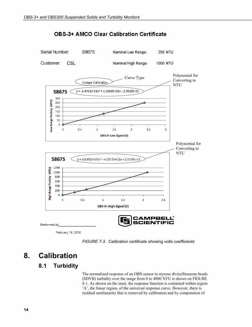
7.5 Calibration Certificate The polynomial for converting to NTU is at the top of each curve and is in the form of:

NTUS = A(X)2 + B(X) + C

Where

A, B, C are provided on the Calibration (see FIGURE 7-2 and FIGURE 7-3).

X = millivolts or volts depending on the curve you are using.

CAUTION


13

FIGURE 7-2. Calibration certificate showing millivolt coefficients

Curve Type Polynomial for Converting to NTU

Polynomial for Converting to NTU

CSL


14

FIGURE 7-3. Calibration certificate showing volts coefficients

8. Calibration 8.1 Turbidity

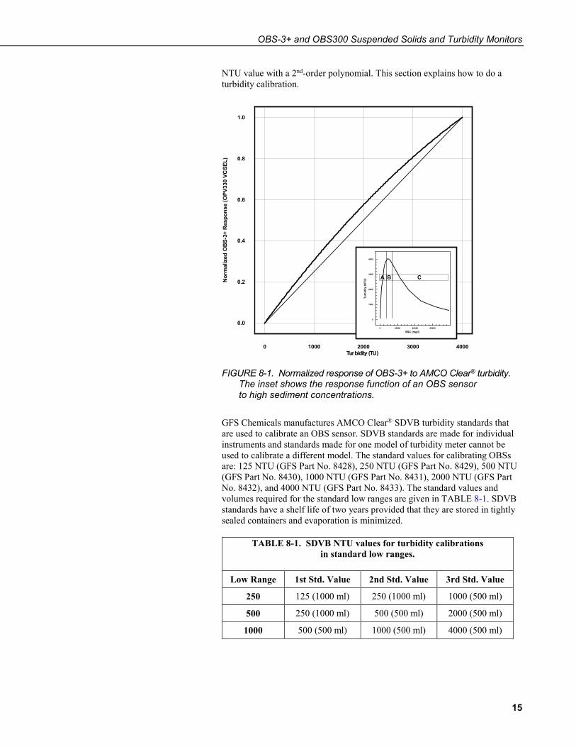
The normalized response of an OBS sensor to styrene divinylbenzene beads (SDVB) turbidity over the range from 0 to 4000 NTU is shown on FIGURE 8-1. As shown on the inset, the response function is contained within region ‘A’, the linear region, of the universal response curve. However, there is residual nonlinearity that is removed by calibration and by computation of



Curve Type

CSL


15

NTU value with a 2nd-order polynomial. This section explains how to do a turbidity calibration.

0 1000 2000 3000 4000Turbidity (TU)

0.0

0.2

0.4

0.6

0.8

1.0

Nor

mal

ized

OB

S-3+

Res

pons

e (O

PV33

0 VC

SEL)

FIGURE 8-1. Normalized response of OBS-3+ to AMCO Clear® turbidity. The inset shows the response function of an OBS sensor to high sediment concentrations.

GFS Chemicals manufactures AMCO Clear® SDVB turbidity standards that are used to calibrate an OBS sensor. SDVB standards are made for individual instruments and standards made for one model of turbidity meter cannot be used to calibrate a different model. The standard values for calibrating OBSs are: 125 NTU (GFS Part No. 8428), 250 NTU (GFS Part No. 8429), 500 NTU (GFS Part No. 8430), 1000 NTU (GFS Part No. 8431), 2000 NTU (GFS Part No. 8432), and 4000 NTU (GFS Part No. 8433). The standard values and volumes required for the standard low ranges are given in TABLE 8-1. SDVB standards have a shelf life of two years provided that they are stored in tightly sealed containers and evaporation is minimized.

TABLE 8-1. SDVB NTU values for turbidity calibrations in standard low ranges.

Low Range 1st Std. Value 2nd Std. Value 3rd Std. Value

250 125 (1000 ml) 250 (1000 ml) 1000 (500 ml)

500 250 (1000 ml) 500 (500 ml) 2000 (500 ml)

1000 500 (500 ml) 1000 (500 ml) 4000 (500 ml)

0 20000 40000 60000

SSC (mg/l)

0

1000

2000

3000

4000

Turb

idity

(NTU

) A B C


16

The NTU values of the standards will remain the same as long as the ratio of particle mass (number of particles) to water mass (volume) does not change. Evaporation causes this ratio to increase and dust, bacteria growth, and dirty glassware can also cause it to increase. Therefore:

1. Always use clean glassware and calibration containers.

2. Don’t leave standards on the bench in open containers or leave the standard bottles uncapped. Perform the calibration as quickly as possible and return the AMCO solutions to their bottles.

3. Clean dirty sensors with a clean, alcohol-soaked cloth to sterilize it before dipping it into the standards.

4. Transfer entire bottles between containers, avoiding aeration and shaking excess fluid off the glassware.

Because of the intrinsic errors in the NTU value of formazin used by the SDVB manufacture (GFS Chemicals) and the dilution procedures, the uncertainty in the NTU value of an SDVB standard is ± 1% of the value indicated on the standard bottle. Consequently, the NTU value of one liter of standard in an uncovered 100 mm calibration cup will increase ~ 1% in 10 hours on a typical summer day (R.H. = 90% and air temp. = 18o C). For example, the NTU value of a 2000 NTU standard in a 100-mm cup will increase by about 2 NTU (0.1%) per hour. TABLE 8-2 gives the increases for some other, commonly used standards.

TABLE 8-2. Change in NTU value resulting from one hour of evaporation1 of SDVB standard; in other words, loss of water but not

particles.

Nominal NTU Value

Calibration-cup Size ∅ mm (∅ in.) 250 500 2000 4000

100 (4) +0.26 +0.52 +2.10 +4.20

150 (6) +0.60 +1.20 +4.80 +9.70

8.1.1 Materials and Equipment • OBS sensor with test cable

• Datalogger or averaging DMM with test leads, 12 V gel cell

• Large black polyethylene plastic tub for measuring the clear-water points

• 100-mm and 200-mm black PE calibration cups

The 100-mm cups are used with standards with NTU values greater than 250 NTU and the 200-mm cups are used with the 125 and 250-NTU standards.


17

8.1.2 Setup 1. Plug the test cable into the OBS sensor; connect the red and black leads to

the battery and clip the DMM or datalogger test leads across the blue (+) and green (–) leads.

2. Swab sensor with an alcohol-soaked towel to sterilize it.

8.1.3 Procedure 1. In a large black tub of fresh tap water, aim the OBS sensor so that it’s the

maximum distance from the sensor optics to the far corner of the tub (see FIGURE 8-2). Record a 10-second average of the low-range output. Record the average output on the calibration log sheet.

2. Swap the DMM or datalogger + test lead to the high-range output lead (white) and record a 10-second average of the high-range output. Record the average output on the calibration log sheet.

FIGURE 8-2. Position of OBS-3+ (left) and OBS300 (right) in clean tap water in big black tub

3. Pour the 1st SDVB standard into the appropriate size cup (see TABLE 8-1 and Section 8.1.1, Materials and Equipment (p. 16)).

4. Position the OBS sensor in the cup as shown on FIGURE 8-3 and record 10-second averages of the low- and high-range outputs. Record the average outputs on the calibration log sheet.

5. Pour the standard back into its container.

6. Wipe sensor with a clean dry towel to remove residual standard.

7. Repeat steps 3, 4, 5, and 6 for the other standards.


18

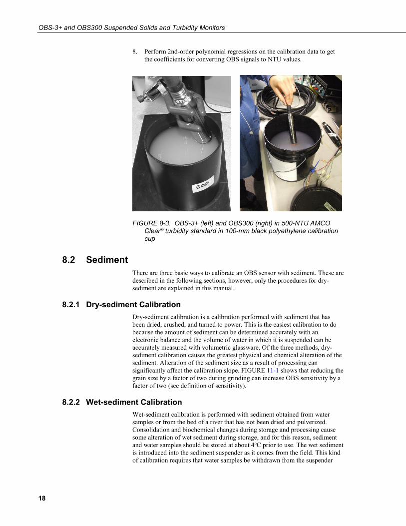
8. Perform 2nd-order polynomial regressions on the calibration data to get the coefficients for converting OBS signals to NTU values.

FIGURE 8-3. OBS-3+ (left) and OBS300 (right) in 500-NTU AMCO Clear® turbidity standard in 100-mm black polyethylene calibration cup

8.2 Sediment There are three basic ways to calibrate an OBS sensor with sediment. These are described in the following sections, however, only the procedures for dry-sediment are explained in this manual.

8.2.1 Dry-sediment Calibration Dry-sediment calibration is a calibration performed with sediment that has been dried, crushed, and turned to power. This is the easiest calibration to do because the amount of sediment can be determined accurately with an electronic balance and the volume of water in which it is suspended can be accurately measured with volumetric glassware. Of the three methods, dry-sediment calibration causes the greatest physical and chemical alteration of the sediment. Alteration of the sediment size as a result of processing can significantly affect the calibration slope. FIGURE 11-1 shows that reducing the grain size by a factor of two during grinding can increase OBS sensitivity by a factor of two (see definition of sensitivity).

8.2.2 Wet-sediment Calibration Wet-sediment calibration is performed with sediment obtained from water samples or from the bed of a river that has not been dried and pulverized. Consolidation and biochemical changes during storage and processing cause some alteration of wet sediment during storage, and for this reason, sediment and water samples should be stored at about 4oC prior to use. The wet sediment is introduced into the sediment suspender as it comes from the field. This kind of calibration requires that water samples be withdrawn from the suspender


19

after each addition of sediment for the determination of SSC by filtration and gravimetric analyses.

8.2.3 In situ Calibration In situ calibration is performed with water samples taken from the immediate vicinity of an OBS sensor in the field over sufficient time to sample the full range of SSC values to which a sensor will be exposed. SSC values obtained for these samples with concurrent recorded OBS sensor signals and regression analysis establishes the mathematical relation for future SSC conversions by an instrument. This is the best sediment-calibration method because the particles are not altered from their natural form in the river (see Lewis, 1996). It is also the most tedious, expensive, and time-consuming method. It can take several years of water sampling with concurrent OBS measurements to record the full range of SSC values on a large river.

8.2.3.1 Materials and Equipment

• OBS sensor with test cable

• Dry, disaggregated sediment from the location where the OBS sensor will be used (sediment should be in a state where grinding, sieving, or pulverization does not change its particle-size distribution)

• Averaging DMM or datalogger with test leads, 12 V gel cell

• Sediment suspender (if a suspender is not available, use a 200-mm I.D. dark plastic container and a drill motor with paint-mixing propeller)

• Electronic balance calibrated with ten-mg accuracy

• 20-ml weigh boats

• Large black polyethylene plastic tub for measuring the clear-water points

• 1-liter, class-A, volumetric flask

• Tea cup with round bottom

• Teaspoon

8.2.3.2 Setup 1. Check the balance with calibration weights; recalibrate if necessary.

2. Plug the test cable to the OBS sensor; connect the red and black leads to the battery and clip the DMM or datalogger test leads across the blue (+) and green (–) leads.

3. Add three liters of tap water to the suspender tub with the volumetric flash.

4. After measuring the clear-water signal (Step 1, Section 8.1.3, Procedure (p. 17)), mount the sensor in the suspender tub. The sensor placement depends on whether the sensor is an OBS-3+ or an OBS300. For the OBS-3+, mount the sensor so that its end is 50 mm above the bottom of the suspender tub and then secure it in a position that minimizes reflections


20

from the wall; see FIGURE 8-4. For the OBS300, mount the sensor so that the laser diode is submerged just below the water surface to maximize the distance from the detector and the bottom of the container.

FIGURE 8-4. Portable sediment suspender (left) and OBS beam orientation in suspender tub (right)

SSC = Wts [Vw + Wts/ρs]–1; where: Wts = total sediment weight in tub, in mg; Vw = volume of water in liters; ρ = density of water (ρ = 1.0 kg l–1 at 10o C); and ρs = sediment density (assume 2.65 103 mg L–1);

8.2.3.3 Procedure 1. Record and log the clean-water signal as in Step 1, Section 8.1.3,

Procedure (p. 17); see FIGURE 8-2.

2. Move the OBS sensor to the suspender as described in setup.

3. Weigh 500 ± 10 mg of sediment in a weigh boat and transfer it to the teacup. Record the weight on the calibration log sheet and add about 10 cc of water from the suspender tub to the teacup and mix the water and sediment into a smooth slurry with the teaspoon.

4. Add the sediment slurry to the tub and rinse the teacup and spoon with tub water to get all the material into the suspender.

5. Turn the suspender ON and let it run for 10 minutes or until the OBS signal stabilizes.

6. Take one-minute averages of the low- and high-range signals with the DMM or datalogger and enter them on the calibration log sheet.

7. Calculate the sediment-weight increment as follows: Wi = 2500 mg (RNG/Vx); where: W i = the incremental weight of sediment, RNG = the range of the OBS sensor (2.5V, 5V, or 16 mA), and Vx = the average output signal from step 6. Note: if the output is 4-20 mA, Vx will equal the output minus 4 mA. The resulting weight gives the amount of sediment to add to get five evenly spaced calibration points.


21

8. Add enough additional sediment to get one full increment of sediment, Wi ± 5%. Repeat steps 4, 5, and 6.

9. Repeat step 8 until five full increments of sediment have been added or until the OBS signals exceed the output range.

10. Perform third-order polynomial regressions on the data to get the coefficients for converting OBS output to SSC.

9. Troubleshooting Do not use a sensor with a stainless steel housing in seawater. This will void the warranty and cause corrosion and leakage.

Do the following tests and see TABLE 9-1 to diagnose an OBS sensor:

1. The Finger-Wave Test is used to determine if an OBS sensor is ‘alive’. Power the OBS sensor and connect a DMM across the low- or high-range output leads (see Section 8.1.2, Setup (p. 17)). Wave your finger across the sensor window about 20 mm away from it. The DMM should show the output fluctuating from a few mV to the full-scale signal. If there are no signal fluctuations of this order, there is a problem that requires attention.

2. The Shake Test is done to determine if water has leaked inside the pressure housing. Unplug the cable and gently shake the sensor next to your ear and listen for sloshing water. This test gives a false negative result when the amount of water in the housing is large enough to destroy the circuit but too small to be audible.

3. A Calibration Check is done to verify if a working OBS sensor needs to be recalibrated. In order to be meaningful, the user must have a criterion for this test. For example, this criterion might be 5%. The sensor is placed in calibration standards with the 1st and 2nd NTU values listed in TABLE 8-1 and the DMM readings are logged. If either reading differs by more than 5% from ones reported on the factory calibration certificate, or the user own calibration data, the sensor should be recalibrated. If the first two calibration points fall within the acceptance criterion, then the third value can be tested. The recommended frequency for calibration checks is quarterly when an OBS sensor is in regular use. Otherwise it should be performed prior to use. Calibration checks can be done in the field.

WARNING


22

TABLE 9-1. Troubleshooting Chart

Fault Cause of Fault Remedy

Fails finger wave test No power, dead battery Replace battery and reconnect wires

MCIL-5 plug not fully seated Disconnect and reinsert plug.

Sensor broken Visually inspect for cracks. Return the sensor to manufacturer if cracks are found.

Electronic failure. Units draws less than 11 mA or more than 40 mA.

Return the sensor to manufacturer.

Fails shake test Sensor leaked Return the sensor to manufacturer.

Fails calibration check Aging of light source causes it to get dimmer with time.

Recalibrate (see Section 8, Calibration (p. 14))

10. Maintenance There are no user-serviceable parts inside the sensor housing. Do not remove the sensor or connector from the pressure housing. This will void the warranty and could cause a leak.

The most important maintenance item is keeping the window clean. A Scotch-Brite scouring pad works well for most types of window fouling. First wet the pad and then place it on a counter with a plastic-laminate top so that the side of the pad is aligned with the edge of the counter. Work the window of the OBS sensor back and forth on the pad until it is clean while removing as little epoxy as possible. If encrusting organisms such as barnacles or tube worms have attached to the sensor, it will have to be gently scraped with a flexible knife blade prior to using the pad. Some applications will result in pitting of the sensor face. Pits can be removed with abrasive cloth. Polish the sensor window as follows:

1. Tape a strip of 400 grit wet-or-dry abrasive cloth to the edge of a counter (see above).

2. Add a few drops of water to the abrasive and work the sensor window in smooth one-way strokes on the cloth using the counter edge as a guide.

3. Continue until the sensor is shiny and pit free.

It is important to remove as little epoxy as possible.

Do not use solvents such as MEK, toluene, acetone, or trichloroethylene on OBS sensors.

WARNING

NOTE

WARNING


23

11. Factors that Affect Turbidity and Suspended-Sediment Measurements

This section summarizes some of the factors that affect OBS measurements and shows how ignoring them can lead to erroneous data. If you are certain that the characteristics of suspended matter will not change during your survey and that your OBS was factory calibrated with sediment from your survey site, you only need to skim this section to confirm that no problems have been over looked.

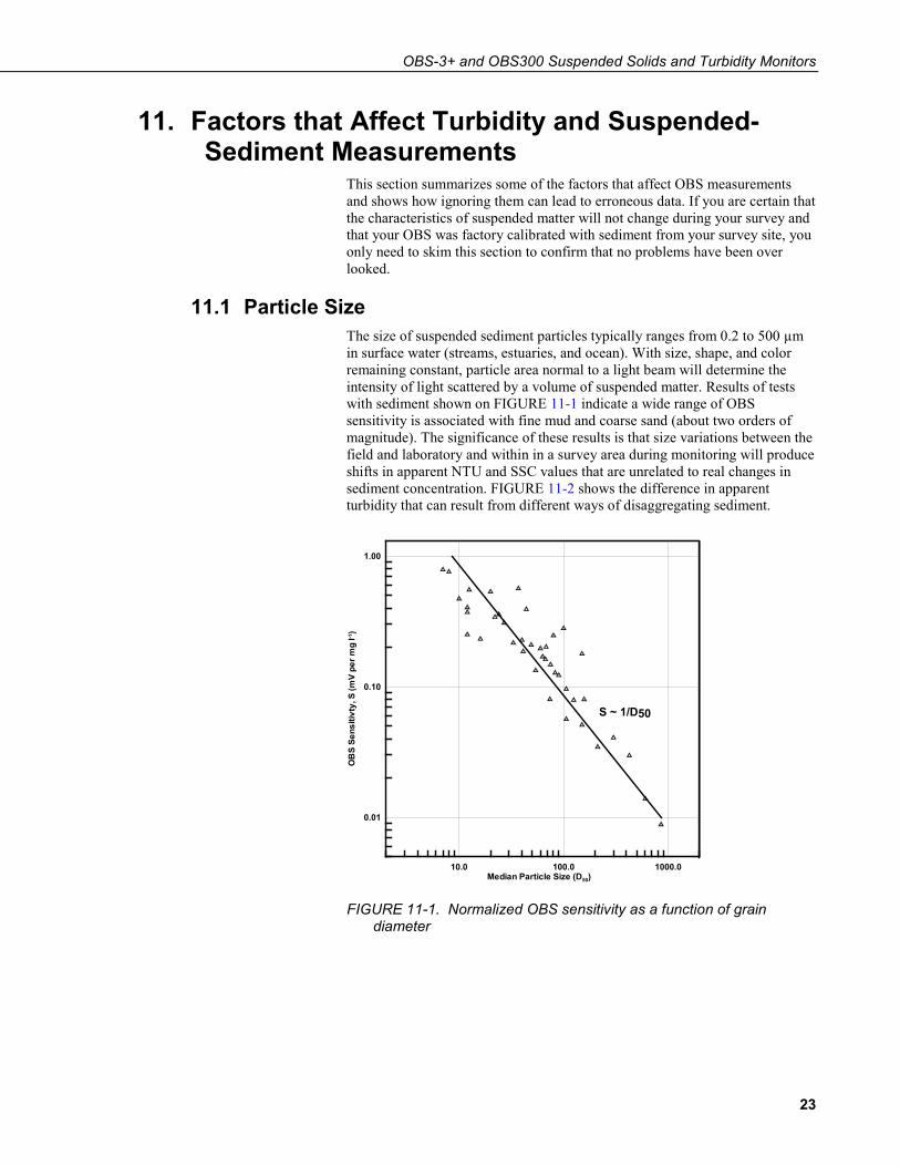
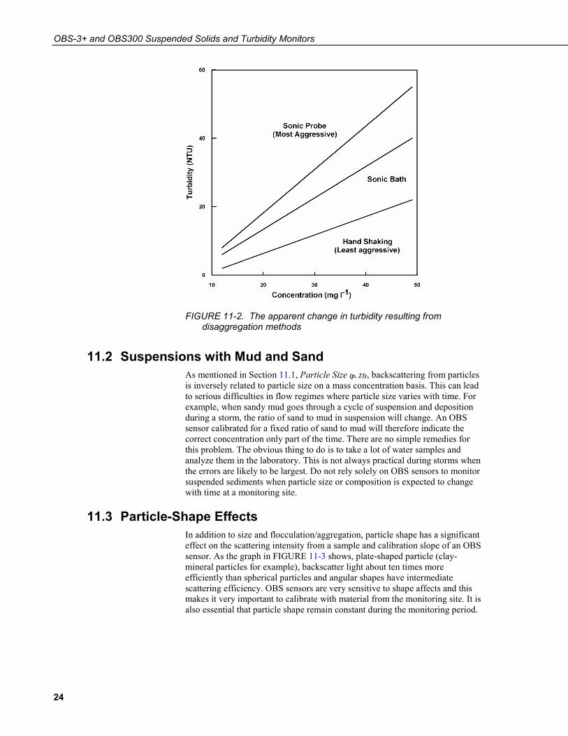
11.1 Particle Size The size of suspended sediment particles typically ranges from 0.2 to 500 µm in surface water (streams, estuaries, and ocean). With size, shape, and color remaining constant, particle area normal to a light beam will determine the intensity of light scattered by a volume of suspended matter. Results of tests with sediment shown on FIGURE 11-1 indicate a wide range of OBS sensitivity is associated with fine mud and coarse sand (about two orders of magnitude). The significance of these results is that size variations between the field and laboratory and within in a survey area during monitoring will produce shifts in apparent NTU and SSC values that are unrelated to real changes in sediment concentration. FIGURE 11-2 shows the difference in apparent turbidity that can result from different ways of disaggregating sediment.

10.0 100.0 1000.0Median Particle Size (D50)

0.01

0.10

1.00

OB

S Se

nsiti

vty,

S (m

V pe

r mg

l-1)

S ~ 1/D50

FIGURE 11-1. Normalized OBS sensitivity as a function of grain diameter


24

FIGURE 11-2. The apparent change in turbidity resulting from disaggregation methods

11.2 Suspensions with Mud and Sand As mentioned in Section 11.1, Particle Size (p. 23), backscattering from particles is inversely related to particle size on a mass concentration basis. This can lead to serious difficulties in flow regimes where particle size varies with time. For example, when sandy mud goes through a cycle of suspension and deposition during a storm, the ratio of sand to mud in suspension will change. An OBS sensor calibrated for a fixed ratio of sand to mud will therefore indicate the correct concentration only part of the time. There are no simple remedies for this problem. The obvious thing to do is to take a lot of water samples and analyze them in the laboratory. This is not always practical during storms when the errors are likely to be largest. Do not rely solely on OBS sensors to monitor suspended sediments when particle size or composition is expected to change with time at a monitoring site.

11.3 Particle-Shape Effects In addition to size and flocculation/aggregation, particle shape has a significant effect on the scattering intensity from a sample and calibration slope of an OBS sensor. As the graph in FIGURE 11-3 shows, plate-shaped particle (clay-mineral particles for example), backscatter light about ten times more efficiently than spherical particles and angular shapes have intermediate scattering efficiency. OBS sensors are very sensitive to shape affects and this makes it very important to calibrate with material from the monitoring site. It is also essential that particle shape remain constant during the monitoring period.


25

0 20 40 60 80 100 120 140 160 180

Scattering Angle

0.01

0.1

1

Rel

ativ

e Sc

atte

ring

Inte

nsity

Cubes

Plates

Spheres

OBS-3+

FIGURE 11-3. Relative scattering intensities of grain shapes

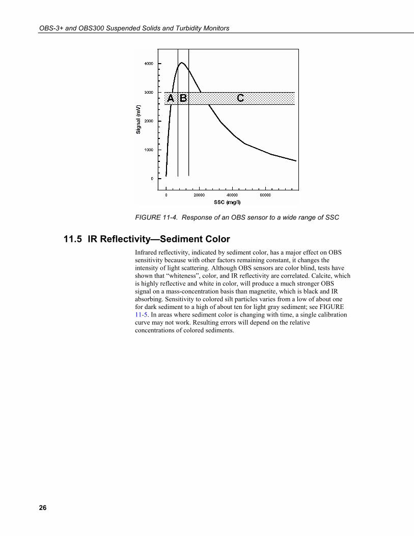
11.4 High Sediment Concentrations At high sediment concentrations, particularly in suspensions of clay and silt, the infrared radiation from the emitter can be so strongly attenuated along the path connecting the emitter, the particle, and the detector, that backscatter decreases exponentially with increasing sediment concentration. For mud, this occurs at concentrations greater than about 5000 mg L–1. FIGURE 11-4 shows a calibration in which sediment concentrations exceeding 6,000 mg L–1 cause the output signal to decrease. It is recommended not to exceed the specified turbidity or suspended sediment ranges, otherwise the interpretation of the signal can be ambiguous. For example, a signal level of 2000 mV (FIGURE 11-4) could be interpreted to indicate SSC values of either 3,000 or 33,000 mg L–1. Factory calibrations are performed in the linear region designated ‘A’ on the graph.


26

FIGURE 11-4. Response of an OBS sensor to a wide range of SSC

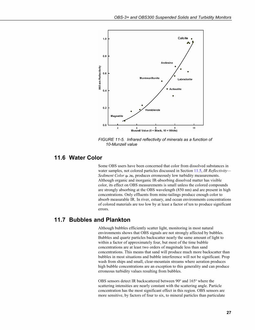
11.5 IR Reflectivity—Sediment Color Infrared reflectivity, indicated by sediment color, has a major effect on OBS sensitivity because with other factors remaining constant, it changes the intensity of light scattering. Although OBS sensors are color blind, tests have shown that “whiteness”, color, and IR reflectivity are correlated. Calcite, which is highly reflective and white in color, will produce a much stronger OBS signal on a mass-concentration basis than magnetite, which is black and IR absorbing. Sensitivity to colored silt particles varies from a low of about one for dark sediment to a high of about ten for light gray sediment; see FIGURE 11-5. In areas where sediment color is changing with time, a single calibration curve may not work. Resulting errors will depend on the relative concentrations of colored sediments.


27

FIGURE 11-5. Infrared reflectivity of minerals as a function of 10-Munzell value

11.6 Water Color Some OBS users have been concerned that color from dissolved substances in water samples, not colored particles discussed in Section 11.5, IR Reflectivity—Sediment Color (p. 26), produces erroneously low turbidity measurements. Although organic and inorganic IR-absorbing dissolved matter has visible color, its effect on OBS measurements is small unless the colored compounds are strongly absorbing at the OBS wavelength (850 nm) and are present in high concentrations. Only effluents from mine-tailings produce enough color to absorb measurable IR. In river, estuary, and ocean environments concentrations of colored materials are too low by at least a factor of ten to produce significant errors.

11.7 Bubbles and Plankton Although bubbles efficiently scatter light, monitoring in most natural environments shows that OBS signals are not strongly affected by bubbles. Bubbles and quartz particles backscatter nearly the same amount of light to within a factor of approximately four, but most of the time bubble concentrations are at least two orders of magnitude less than sand concentrations. This means that sand will produce much more backscatter than bubbles in most situations and bubble interference will not be significant. Prop wash from ships and small, clear-mountain streams where aeration produces high bubble concentrations are an exception to this generality and can produce erroneous turbidity values resulting from bubbles.

OBS sensors detect IR backscattered between 90o and 165o where the scattering intensities are nearly constant with the scattering angle. Particle concentration has the most significant effect in this region. OBS sensors are more sensitive, by factors of four to six, to mineral particles than particulate


28

organic matter and interference from these materials can therefore be ignored most of the time. One notable exception is where biological productivity is high and sediment production from rivers and re-suspension is low. In such an environment, OBS signals can come predominately from plankton.

11.8 Biological and Chemical Fouling Sensor cleaning is essential during extended deployments. In salt water, barnacle growth on an OBS sensor can obscure the IR emitter, the detector, or both and produce an apparent decline in turbidity. Algal growth in marine and fresh waters has caused spurious scatter and apparent increases of OBS output. The reverse has also been noted in fresh water where the signal increases after cleaning the sensor window. Prolonged operation in freshwater with high tannin levels can cause a varnish-like coating to develop on an OBS sensor that obscures the IR emitter and caused an apparent decline in turbidity. Cleaning algal and tannin accumulation off OBS sensors is required more often during the summer because warm water and bright sunlight increase biological and chemical activity.

Campbell Scientific sells two wipers from a third-party manufacturer: the Hydro-Wiper C with its own controller, or the Hydro-Wiper D that is controlled by a datalogger.

12. References Bohren, C.F. and D.H. Huffman. Absorption and Scattering of Light by Small Particles, John Wiley & Sons, New York, 1983.

Downing, John. 2006. Twenty-five Years with OBS Sensors: the Good, the Bad, and the Ugly. Continental Shelf Research 26, 2299-2318.

Downing, John, Turbidity Monitoring, Chapter 24 In: Environmental Instrumentation and Analysis Handbook, John Wiley & Sons, New York, pp. 511-546, 2005.

Downing, John and R.A. Beach. 1989. Laboratory apparatus for calibrating optical suspended solids sensors. Marine Geology 86, 243-249.

Lewis, Jack. 1996. Turbidity-controlled Suspended Sediment Sampling for Runoff-event Load Estimation. Water Resources Research, 32(7), pp. 2299-2310.

Sadar, M. 1998. Turbidity Standards. Hach Company Technical Information Series – Booklet No. 12. 18 pages.

Sutherland T.F., P.M. Lane, C.L. Amos, and John Downing. 2000. The Calibration of Optical Backscatter Sensors for Suspended Sediment of Varying Darkness Level. Marine Geology, 162, pp. 587-597.

U.S. Geological Survey. 2005. National Field Manual of the Collection of Water-Quality Data. Book 9, Handbooks for Water-Resources Investigations

Zaneveld, J.R.V., R.W. Spinrad and R. Bartz. 1979. Optical Properties of Turbidity Standards. SPIE 208 Ocean Optics VI. Bellingham, Washington, pp. 159-158, 1979.


29

13. Terminology 110 Rule: 100 ppm of 100-μm suspended sand will scatter light with the same intensity as 10 ppm of 10-μm suspended silt, other factors, such as size, shape and color, remaining constant.

Backscatter/forward scatter: The interaction of light with suspended particles, water molecules, and variations in refractive index that alters the direction of light transport through a sample without changing the wavelength. The angle between the direction of propagation of a source light beam and the direction of a scattered beam is the scattering angle. Forward-scattering refers to scattering angles less than 90º and backscattering refers scattering angle equal to or greater than 90º.

Calibration Slope: NTU or SSC value per mV or mA of OBS output. It is nearly constant in the linear region of the OBS response function but is a function of sediment concentration elsewhere.

Daylight-Rejection Filter: An optical bandpass filter that transmits near infrared light (760 to 1200 nm) and blocks visible light (390 to 760 nm).

Drift: A change in OBS output over time or with ambient temperature that is unrelated to the sample turbidity or SSC.

Interference: Properties of the sample, the environment, or measurement procedure that produce unintended and unknown shifts in turbidity or SSC.

Sample Volume: The water volume where the OBS infrared beam and suspended particles interact and the scattered light is detected. OBS sample volumes range from 25 to 12 x 104 mm3, i.e. BBs to tennis balls, depending on turbidity.

SDVB: Styrene divinylbenzene beads, a calibration solution also known as AMCO Clear®.

Sensitivity: The ratio of output level (mV, mA, or NTU value) to suspended-sediment concentration; for example, mV per mg L–1, mA per mg L–1, or NTU per mg L–1.

Suspended-Sediment Concentration (SSC): Mass or volume of sediment in a sample divided by the volume (or weight) of the sample expressed as mg L–1

(or ppm).

Synchronous Detection: A signal-processing technique for rejecting d.c. shifts wherein the gain is switched from –1 to 1 synchronously with the OBS clock. This technique limits the bandwidth and noise of a circuit.

Temperature Coefficient: The change in OBS output per unit of ambient temperature change expressed as ppm. For example, an OBS that indicates 100 NTU in a standard at 25o C and 101 NTU in the same standard at 5oC would have a temperature coefficient of –500 ppm.

Turbidity (conceptual definition): A numerical expression, in relative units, of the optical properties that cause water to appear hazy or cloudy when light to be scattered and absorbed by suspended matter. Turbidity is caused by


30

sediment, plankton, bacteria and viruses, organic acids, and dyes. In general, as the concentration of suspended matter increases, so will water turbidity, and as the concentration of dissolved light-absorbing matter increases, turbidity will decrease.

Turbidity (operational definition): NTU value is a number ranging from 0 to 10,000 that is computed by a turbidimeter from measurements of the intensity of light scattered from water sample and by interpolation between bracketing SDVB (AMCO Clear®) calibration values.

A-1

Appendix A. Importing Short Cut Code Into CRBasic Editor

This tutorial shows:

• How to import a Short Cut program into a program editor for additional refinement

• How to import a wiring diagram from Short Cut into the comments of a custom program

Short Cut creates files, which can be imported into CRBasic Editor. Assuming defaults were used when Short Cut was installed, these files reside in the C:\campbellsci\SCWin folder:

• .DEF (wiring and memory usage information) • .CR2 (CR200(X)-series datalogger code) • .CR300 (CR300-series datalogger code) • .CR6 (CR6-series datalogger code) • .CR8 (CR800-series datalogger code) • .CR1 (CR1000 datalogger code) • .CR3 (CR3000 datalogger code) • .CR5 (CR5000 datalogger code) • .CR9 (CR9000(X) datalogger code)

Use the following procedure to import Short Cut code and wiring diagram into CRBasic Editor.

1. Create the Short Cut program following the procedure in Section 4, QuickStart (p. 2). Finish the program and exit Short Cut. Make note of the file name used when saving the Short Cut program.

2. Open CRBasic Editor.

3. Click File | Open. Assuming the default paths were used when Short Cut was installed, navigate to C:\CampbellSci\SCWin folder. The file of interest has the .CR2, .CR300, .CR8, .CR1, .CR3, .CR5, or .CR9 extension. Select the file and click Open.

4. Immediately save the file in a folder different from C:\Campbellsci\SCWin, or save the file with a different file name.

Once the file is edited with CRBasic Editor, Short Cut can no longer be used to edit the datalogger program. Change the name of the program file or move it, or Short Cut may overwrite it next time it is used.

5. The program can now be edited, saved, and sent to the datalogger.

6. Import wiring information to the program by opening the associated .DEF file. Copy and paste the section beginning with heading “-Wiring for CRXXX–” into the CRBasic program, usually at the head of the file. After pasting, edit the information such that an apostrophe (') begins each line. This character instructs the datalogger compiler to ignore the line when compiling.

NOTE

B-1

Appendix B. Example Programs B.1 CR1000 Example Program

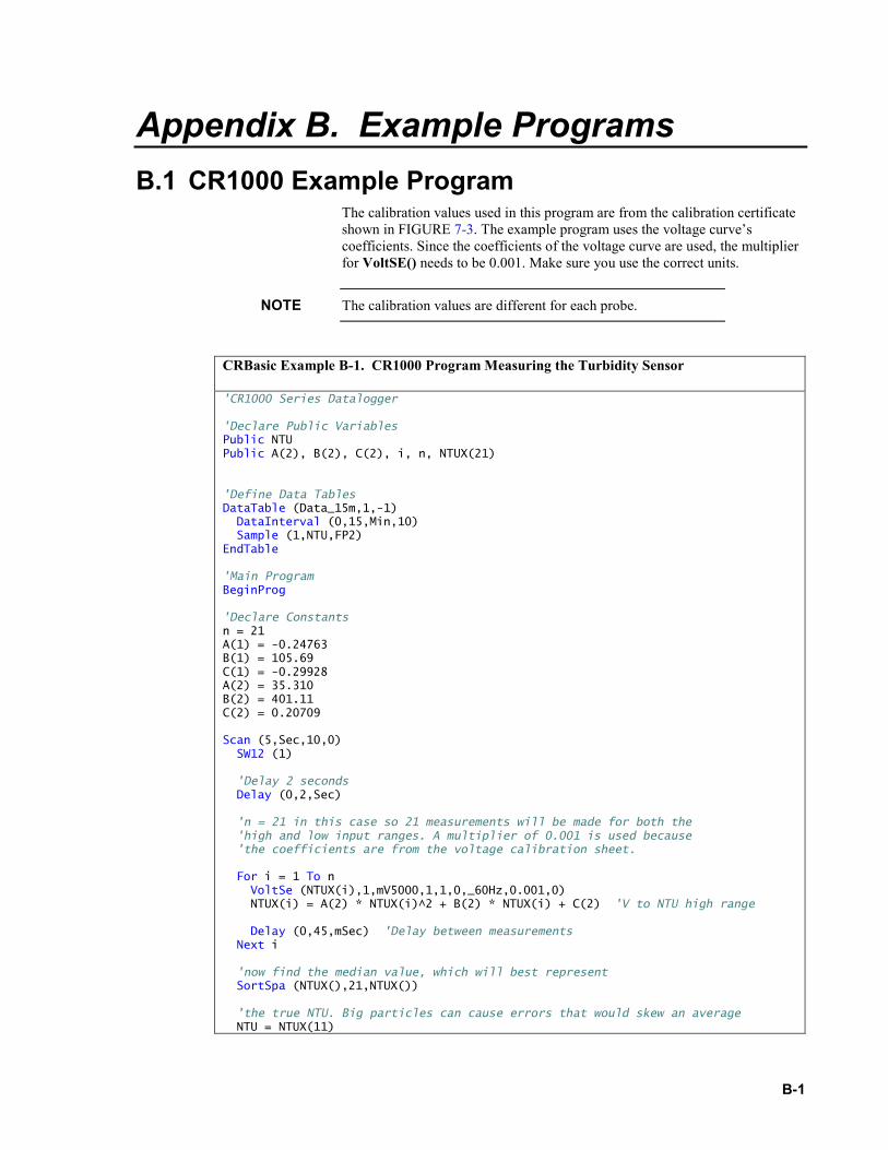
The calibration values used in this program are from the calibration certificate shown in FIGURE 7-3. The example program uses the voltage curve’s coefficients. Since the coefficients of the voltage curve are used, the multiplier for VoltSE() needs to be 0.001. Make sure you use the correct units.

The calibration values are different for each probe.

CRBasic Example B-1. CR1000 Program Measuring the Turbidity Sensor

'CR1000 Series Datalogger 'Declare Public Variables Public NTU Public A(2), B(2), C(2), i, n, NTUX(21) 'Define Data Tables DataTable (Data_15m,1,-1) DataInterval (0,15,Min,10) Sample (1,NTU,FP2) EndTable 'Main Program BeginProg 'Declare Constants n = 21 A(1) = -0.24763 B(1) = 105.69 C(1) = -0.29928 A(2) = 35.310 B(2) = 401.11 C(2) = 0.20709 Scan (5,Sec,10,0) SW12 (1) 'Delay 2 seconds Delay (0,2,Sec) 'n = 21 in this case so 21 measurements will be made for both the 'high and low input ranges. A multiplier of 0.001 is used because 'the coefficients are from the voltage calibration sheet. For i = 1 To n VoltSe (NTUX(i),1,mV5000,1,1,0,_60Hz,0.001,0) NTUX(i) = A(2) * NTUX(i)^2 + B(2) * NTUX(i) + C(2) 'V to NTU high range Delay (0,45,mSec) 'Delay between measurements Next i 'now find the median value, which will best represent SortSpa (NTUX(),21,NTUX()) 'the true NTU. Big particles can cause errors that would skew an average NTU = NTUX(11)

NOTE

Appendix B. Example Programs

B-2

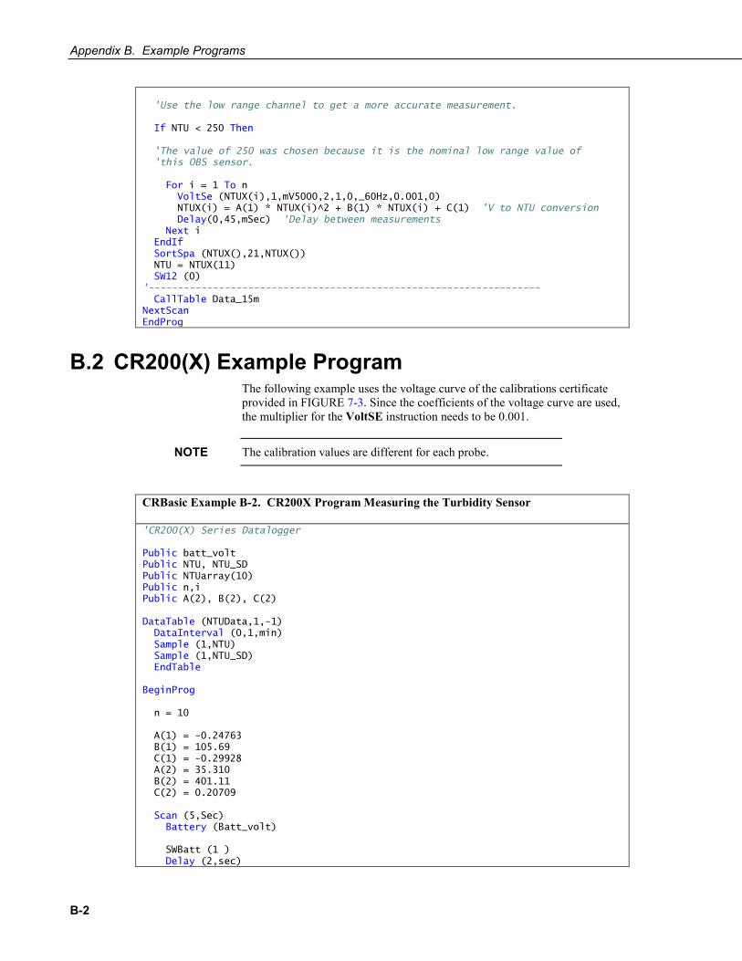
'Use the low range channel to get a more accurate measurement. If NTU < 250 Then 'The value of 250 was chosen because it is the nominal low range value of 'this OBS sensor. For i = 1 To n VoltSe (NTUX(i),1,mV5000,2,1,0,_60Hz,0.001,0) NTUX(i) = A(1) * NTUX(i)^2 + B(1) * NTUX(i) + C(1) 'V to NTU conversion Delay(0,45,mSec) 'Delay between measurements Next i EndIf SortSpa (NTUX(),21,NTUX()) NTU = NTUX(11) SW12 (0) '------------------------------------------------------------------- CallTable Data_15m NextScan EndProg

B.2 CR200(X) Example Program The following example uses the voltage curve of the calibrations certificate provided in FIGURE 7-3. Since the coefficients of the voltage curve are used, the multiplier for the VoltSE instruction needs to be 0.001.

The calibration values are different for each probe.

CRBasic Example B-2. CR200X Program Measuring the Turbidity Sensor

'CR200(X) Series Datalogger Public batt_volt Public NTU, NTU_SD Public NTUarray(10) Public n,i Public A(2), B(2), C(2) DataTable (NTUData,1,-1) DataInterval (0,1,min) Sample (1,NTU) Sample (1,NTU_SD) EndTable BeginProg n = 10 A(1) = -0.24763 B(1) = 105.69 C(1) = -0.29928 A(2) = 35.310 B(2) = 401.11 C(2) = 0.20709 Scan (5,Sec) Battery (Batt_volt) SWBatt (1 ) Delay (2,sec)

NOTE


B-3

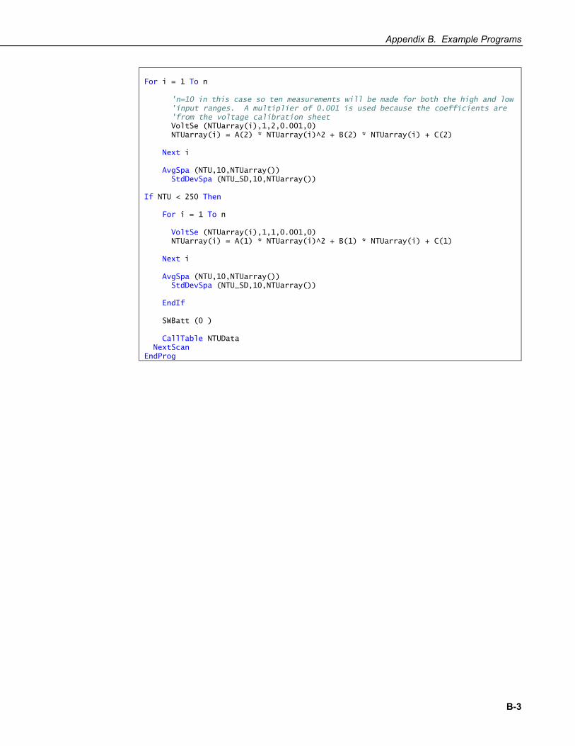
For i = 1 To n 'n=10 in this case so ten measurements will be made for both the high and low 'input ranges. A multiplier of 0.001 is used because the coefficients are 'from the voltage calibration sheet VoltSe (NTUarray(i),1,2,0.001,0) NTUarray(i) = A(2) * NTUarray(i)^2 + B(2) * NTUarray(i) + C(2) Next i AvgSpa (NTU,10,NTUarray()) StdDevSpa (NTU_SD,10,NTUarray()) If NTU < 250 Then For i = 1 To n VoltSe (NTUarray(i),1,1,0.001,0) NTUarray(i) = A(1) * NTUarray(i)^2 + B(1) * NTUarray(i) + C(1) Next i AvgSpa (NTU,10,NTUarray()) StdDevSpa (NTU_SD,10,NTUarray()) EndIf SWBatt (0 ) CallTable NTUData NextScan EndProg


B-4

C-1

Appendix C. Electrical Connections Details

FIGURE C-1 shows the contact numbers for the MCIL/MCBH-5 connectors and TABLE C-1 lists the electrical functions and wire colors. The user need only be concerned with the wire colors for the 8425 cable as the MCBH wires are not accessible. When a custom cable assembly is purchased from a third-party vendor to connect the OBS sensor to a current meter or CTD, the user will not have access to any of the wires listed in TABLE C-1.

FIGURE C-1. Pin assignments for MCBH and MCIL wet-pluggable connectors

MP Face View

GREEN WHITE BLACK BLUE

RED

FS

Appendix C. Electrical Connections Details

C-2

TABLE C-1. Pin numbers, electrical functions and wire color codes for OBS sensor bulkhead connectors.

MCBH-5-FS/MCIL-5-MP Contact Number

Electrical Function

Wire Color (MCBH)

Wire Color (8425)

1 Power (5 – 15V) Red Red

2 Power Ground Black Black

3 Signal Common Green Green

4 High Range Signal (4X) White White

5 Low Range Signal (1X & 4-20 mA) Blue Blue

No Connection Cable Shield Clear/Braid

D-1

Appendix D. Datalogger Connection to a Relay

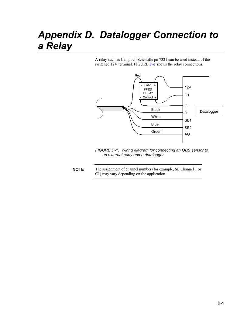
A relay such as Campbell Scientific pn 7321 can be used instead of the switched 12V terminal. FIGURE D-1 shows the relay connections.

12V

C1

G

G

SE1

SE2

AG

Black

White

Blue

Green

FIGURE D-1. Wiring diagram for connecting an OBS sensor to an external relay and a datalogger

The assignment of channel number (for example, SE Channel 1 or C1) may vary depending on the application.

NOTE

Campbell Scientific Companies

Campbell Scientific, Inc. 815 West 1800 North Logan, Utah 84321 UNITED STATES

www.campbellsci.com • [email protected]

Campbell Scientific Africa Pty. Ltd. PO Box 2450

Somerset West 7129 SOUTH AFRICA

www.campbellsci.co.za • [email protected]

Campbell Scientific Southeast Asia Co., Ltd. 877/22 Nirvana@Work, Rama 9 Road

Suan Luang Subdistrict, Suan Luang District Bangkok 10250

THAILAND www.campbellsci.asia • [email protected]

Campbell Scientific Australia Pty. Ltd. PO Box 8108

Garbutt Post Shop QLD 4814 AUSTRALIA

www.campbellsci.com.au • [email protected]

Campbell Scientific (Beijing) Co., Ltd. 8B16, Floor 8 Tower B, Hanwei Plaza

7 Guanghua Road Chaoyang, Beijing 100004

P.R. CHINA www.campbellsci.com • [email protected]

Campbell Scientific do Brasil Ltda. Rua Apinagés, nbr. 2018 ─ Perdizes CEP: 01258-00 ─ São Paulo ─ SP

BRASIL www.campbellsci.com.br • [email protected]

Campbell Scientific Canada Corp. 14532 – 131 Avenue NW Edmonton AB T5L 4X4

CANADA www.campbellsci.ca • [email protected]

Campbell Scientific Centro Caribe S.A. 300 N Cementerio, Edificio Breller

Santo Domingo, Heredia 40305 COSTA RICA

www.campbellsci.cc • [email protected]

Campbell Scientific Ltd. Campbell Park

80 Hathern Road Shepshed, Loughborough LE12 9GX

UNITED KINGDOM www.campbellsci.co.uk • [email protected]

Campbell Scientific Ltd. 3 Avenue de la Division Leclerc

92160 ANTONY FRANCE

www.campbellsci.fr • [email protected]

Campbell Scientific Ltd. Fahrenheitstraße 13

28359 Bremen GERMANY

www.campbellsci.de • [email protected]

Campbell Scientific Spain, S. L. Avda. Pompeu Fabra 7-9, local 1

08024 Barcelona SPAIN

www.campbellsci.es • [email protected]

Please visit www.campbellsci.com to obtain contact information for your local US or international representative.


http://www.campbellsci.co.za/

http://www.campbellsci.asia/

http://www.campbellsci.com.au/


http://www.campbellsci.com.br/

http://www.campbellsci.ca/

http://www.campbellsci.cc/

http://www.campbellsci.co.uk/

http://www.campbellsci.fr/

http://www.campbellsci.de/

http://www.campbellsci.es/

https://www.campbellsci.com/

Documents

OBS-3+ and OBS300 Suspended Solids and Turbidity ….pdf · Limited Warranty “Products manufactured by CSI are warranted by CSI to be free from defects in materials and workmanship