Embed Size (px)
Citation preview

Universidad Politecnica de Madrid
Master’s Thesis
Object tracking using directmethods in RGB-D cameras
Author:
Isaac Sanchez
Supervisor:
Luis Baumela
A thesis submitted in fulfilment of the requirements
for the degree of Master Universitario en Inteligencia Artificial
in the
July 2015

“Every day I remind myself that my inner and outer life are based on the labors of
other men, living and dead, and that I must exert myself in order to give in the same
measure as I have received and am still receiving.”
Albert Einstein

UPM
ResumenEscuela Tecnica Superior de Ingenieros Informaticos
Departamento de Inteligencia Artificial
Master Universitario en Inteligencia Artificial
Seguimiento de objetos mediante metodos directos con camaras RGB-D
por Isaac Sanchez
En esta tesis se presenta un analisis en profundidad de como se deben utilizar dos
tipos de metodos directos, Lucas-Kanade e Inverse Compositional, en imagenes
RGB-D y se analiza la capacidad y precision de los mismos en una serie de ex-
perimentos sinteticos. Estos simulan imagenes RGB, imagenes de profundidad (D)
e imagenes RGB-D para comprobar como se comportan en cada una de las com-
binaciones. Ademas, se analizan estos metodos sin ninguna tecnica adicional que
modifique el algoritmo original ni que lo apoye en su tarea de optimizacion tal y como
sucede en la mayorıa de los artıculos encontrados en la literatura. Esto se hace con
el fin de poder entender cuando y por que los metodos convergen o divergen para
que ası en el futuro cualquier interesado pueda aplicar los conocimientos adquiridos
en esta tesis de forma practica. Esta tesis deberıa ayudar al futuro interesado a
decidir que algoritmo conviene mas en una determinada situacion y deberıa tambien
ayudarle a entender que problemas le pueden dar estos algoritmos para poder poner
el remedio mas apropiado. Las tecnicas adicionales que sirven de remedio para estos
problemas quedan fuera de los contenidos que abarca esta tesis, sin embargo, sı se
hace una revision sobre ellas.

UPM
AbstractEscuela Tecnica Superior de Ingenieros Informaticos
Departamento de Inteligencia Artificial
Master Universitario en Inteligencia Artificial
Object tracking using direct methods in RGB-D cameras
by Isaac Sanchez
This thesis presents an in-depth analysis about how direct methods such as Lucas-
Kanade and Inverse Compositional can be applied in RGB-D images. The capability
and accuracy of these methods is also analyzed employing a series of synthetic ex-
periments. These simulate the effects produced by RGB images, depth images and
RGB-D images so that different combinations can be evaluated. Moreover, these
methods are analyzed without using any additional technique that modifies the
original algorithm or that aids the algorithm in its search for a global optima unlike
most of the articles found in the literature. Our goal is to understand when and why
do these methods converge or diverge so that in the future, the knowledge extracted
from the results presented here can effectively help a potential implementer. After
reading this thesis, the implementer should be able to decide which algorithm fits
best for a particular task and should also know which are the problems that have
to be addressed in each algorithm so that an appropriate correction is implemented
using additional techniques. These additional techniques are outside the scope of
this thesis, however, they are reviewed from the literature.

Agradecimientos
Me gustarıa agradecer a Luis todos los ratos que me ha ayudado a entender la
materia, a sus discusiones y en especial, a su paciencia y sus constantes ganas y
animos que me han llevado a terminar satisfactoriamente este trabajo.
Agradezco tambien a todos los profesores que me han ayudado a progresar en cada
uno de los distintos enfoques que ellos han adoptado sobre la vida, sobre esta ciencia,
la informatica, e incluso de cualquier otra rama de la ciencia en general. Gracias
a ellos, creo tener una mejor capacidad de contrastar ideas, evaluar situaciones y
sobre todo afrontar los problemas con una mayor creatividad. Sin ellos no podrıa
llegar a pensar con la misma claridad con la que a dıa de hoy puedo. Y esto es un
privilegio del que no todo el mundo puede disfrutar.
Doy gracias tambien a toda la comunidad de software libre ya que sin ellos, la
cantidad de informaticos bien formados se habrıa visto impactada considerablemente
al no poder disfrutar de la libertad de enteder el software producido por otros.
Aparte de esto, les doy las gracias puesto que sin sus esfuerzos, la totalidad de las
tareas realizadas en esta tesis no se habrıa podido llevar a cabo.
Doy las gracias a mis padres y a toda mi familia en general puesto que sin su ayuda
ni su apoyo no podrıa haber conseguido ninguno de los objetivos que me he marcado
a lo largo de mi vida. Ademas, no me cabe ninguna duda de que sin la libertad y el
constante apoyo de los que he disfrutado, es muy probable que no hubiese ni siquiera
llegado a elegir y seguir este camino.
Y por supuesto, tambien doy las gracias a todos mis allegados incluyendo a todos
mis amigos, que me han apoyado incondicionalmente y me han acompanado en mis
risas y soportado mis penas.
v


Contents
Resumen iii
Abstract iv
Agradecimientos v
Contents vi
List of Figures xi
Abbreviations xiii
Symbols xv
1 Introduction 1
1.1 Motivation . . . . . . . . . . . . . . . . . . . . . . . . . . . . . . . . . 2
2 Literature review 5
2.1 General misconceptions . . . . . . . . . . . . . . . . . . . . . . . . . . 5
2.2 Image registration techniques . . . . . . . . . . . . . . . . . . . . . . 6
2.2.1 Direct methods . . . . . . . . . . . . . . . . . . . . . . . . . . 6
2.2.2 Feature-based methods . . . . . . . . . . . . . . . . . . . . . . 7
2.3 Other object tracking and detection techniques . . . . . . . . . . . . 7
2.4 Techniques in RGB-D images . . . . . . . . . . . . . . . . . . . . . . 8
vii

Contents viii
3 Background 11
3.1 Models . . . . . . . . . . . . . . . . . . . . . . . . . . . . . . . . . . . 11
3.1.1 2D affine transformations . . . . . . . . . . . . . . . . . . . . 12
3.1.2 3D transformations and pinhole camera model . . . . . . . . . 15
3.2 Direct methods . . . . . . . . . . . . . . . . . . . . . . . . . . . . . . 18
3.2.1 Lucas-Kanade . . . . . . . . . . . . . . . . . . . . . . . . . . . 20
3.2.2 Inverse Compositional . . . . . . . . . . . . . . . . . . . . . . 22
3.2.3 Other notable mentions . . . . . . . . . . . . . . . . . . . . . 25
3.2.4 Additional improvements . . . . . . . . . . . . . . . . . . . . . 25
3.3 RGB-D cameras . . . . . . . . . . . . . . . . . . . . . . . . . . . . . . 28
4 Methodology 31
4.1 The unidimensional case . . . . . . . . . . . . . . . . . . . . . . . . . 31
4.2 Implementation details . . . . . . . . . . . . . . . . . . . . . . . . . . 40
4.2.1 Jacobian calculation . . . . . . . . . . . . . . . . . . . . . . . 40
4.2.1.1 Analytic Jacobian . . . . . . . . . . . . . . . . . . . 41
4.2.1.2 Numeric Jacobian . . . . . . . . . . . . . . . . . . . 45
4.2.1.3 Comparison of Jacobian calculations . . . . . . . . . 46
4.2.2 RGB-D in direct methods . . . . . . . . . . . . . . . . . . . . 49
4.3 Synthetic models . . . . . . . . . . . . . . . . . . . . . . . . . . . . . 55
4.3.1 Finite plane . . . . . . . . . . . . . . . . . . . . . . . . . . . . 56
4.3.2 Simple cube . . . . . . . . . . . . . . . . . . . . . . . . . . . . 56
5 Results 61
5.1 Testing procedure . . . . . . . . . . . . . . . . . . . . . . . . . . . . . 62
5.2 Results analysis . . . . . . . . . . . . . . . . . . . . . . . . . . . . . . 64
5.2.1 Test sets . . . . . . . . . . . . . . . . . . . . . . . . . . . . . . 65
5.2.2 Overall results . . . . . . . . . . . . . . . . . . . . . . . . . . . 71
6 Conclusions 77
6.1 Future work . . . . . . . . . . . . . . . . . . . . . . . . . . . . . . . . 78
A Kinect and OpenCV 81

Contents ix
Bibliography 85

List of Figures
1.1 Localization and mapping image example obtained from https://
groups.csail.mit.edu. . . . . . . . . . . . . . . . . . . . . . . . . . 2
1.2 Video mosaicing image obtained from Google Images. . . . . . . . . . 3
3.1 Classic cameraman image with sample points showing duality. . . . . 14
3.2 Several layers of the pyramid in a coarse-to-fine scheme. . . . . . . . . 27
4.1 Function g is centered at 1 while function f is centered at 0. . . . . . 32
4.2 Residual and its derivatives depending on the parameter µ which isrenamed in the axis as p . . . . . . . . . . . . . . . . . . . . . . . . . 33
4.3 First iteration of the optimisation . . . . . . . . . . . . . . . . . . . . 34
4.4 Second iteration of the optimisation . . . . . . . . . . . . . . . . . . . 36
4.5 Third iteration of the optimisation . . . . . . . . . . . . . . . . . . . 37
4.6 Example of slow convergence . . . . . . . . . . . . . . . . . . . . . . . 38
4.7 Example of no convergence . . . . . . . . . . . . . . . . . . . . . . . . 39
4.8 Texture image used in figure 4.9 (4 Gaussian distributions in 2D). . . 42
4.9 Analytic Jacobian in one parameter generated in various steps. p1 isthe actual Jacobian. . . . . . . . . . . . . . . . . . . . . . . . . . . . 43
4.10 Differences in practice between the analytic and the numeric Jacobian. 48
4.11 Different pointcloud resolutions. . . . . . . . . . . . . . . . . . . . . . 52
4.12 How different coordinate systems affect the derivatives (green for ro-tation derivatives and red for translation derivatives). . . . . . . . . . 55
4.13 Examples of the cube while camera not zoomed in . . . . . . . . . . . 59
4.14 Examples of the cube while camera zoomed in . . . . . . . . . . . . . 60
5.1 Example of a warp discarded because of its error. . . . . . . . . . . . 64
5.2 Graphs showing the relationship between 2D and 3D error distances. 66
5.3 Warp of [0.2, 0.2, 0, 0, 0, 0], original images and their residuals. . . . . 67
xi

List of Figures xii
5.4 Same graph showing this time a warped image made using [0.3, 0.3, 0, 0, 0, 0]as the template. . . . . . . . . . . . . . . . . . . . . . . . . . . . . . . 68
5.5 Comparison of Jacobians in both examples. . . . . . . . . . . . . . . . 69
5.6 Again the same graph but in IC. . . . . . . . . . . . . . . . . . . . . 70
5.7 Comparison of images in the example with parameters [0.3, 0.3, 0, 0, 0, 0]. 71
5.8 Robustness plot . . . . . . . . . . . . . . . . . . . . . . . . . . . . . . 72
5.9 Accuracy plot . . . . . . . . . . . . . . . . . . . . . . . . . . . . . . . 73
5.10 Rate of convergence plot . . . . . . . . . . . . . . . . . . . . . . . . . 73
A.1 The Kinect device. . . . . . . . . . . . . . . . . . . . . . . . . . . . . 81

Abbreviations
RGB-D Red Green Blue - Depth
AAM Active Appearance Model
SLAM Simultaneous Localization And Mapping
ICP Iterative Closest Point
LK Lucas - Kanade algorithm
IC Inverse Compositional algorithm
BCS Brightness Constancy Assumption
EBCS Extended Brightness Constancy Assumption
ToF Time of Flight
xiii


Symbols
P point in world coordinates
PT point in world coordinates after transformation
PC point in camera coordinates
PS point in screen coordinates
T6dof3D 3D rigid body transformation matrix of 6 dof
K camera intrinsics matrix
C camera extrinsics matrix
I input image(s) function(s) or matrix(ces)
T template image function or matrix
x a single point in space
V set of sample points in space
X V in matrix form
D generic function domain
r residual function or matrix
µ single parameter or vector of parameters
P set of available parameters
δµ single parameter increment or vector of increments
xv

Symbols xvi
L linearization function
J Jacobian of the residual function, either function or matrix
T compositionally accumulated transformations in matrix form

A mis padres, Jose y Hortensia
xvii


Chapter 1
Introduction
Object tracking is an interesting field of research with multiple applications that
range from surveillance in public places and military purposes to player pose tracking
in media and entertainment or any sort of human-computer interaction. Object
tracking is also interesting when applied together with object detection to be able
not only to follow objects in images but also to identify these objects in arbitrary
scenes. A special case of object tracking is motion tracking of faces and body gestures
either with or without marks.
Localization is also a very important application that can take advantage of ob-
ject tracking methods in general. Localization usually requires the identification of
the scenario itself rather than a particular object in a scenario. This is useful for
robot’s self-localization so that they can estimate the position or at least the area
where they are located. Localization has another application related to augmented
reality. Localization is required so that the virtual models that are rendered over a
background actually fit with the background’s coordinate system.
1
Chapter 1. Introduction 2
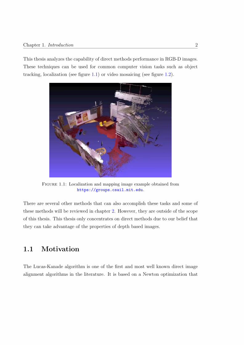
This thesis analyzes the capability of direct methods performance in RGB-D images.
These techniques can be used for common computer vision tasks such as object
tracking, localization (see figure 1.1) or video mosaicing (see figure 1.2).
Figure 1.1: Localization and mapping image example obtained fromhttps://groups.csail.mit.edu.
There are several other methods that can also accomplish these tasks and some of
these methods will be reviewed in chapter 2. However, they are outside of the scope
of this thesis. This thesis only concentrates on direct methods due to our belief that
they can take advantage of the properties of depth based images.
1.1 Motivation
The Lucas-Kanade algorithm is one of the first and most well known direct image
alignment algorithms in the literature. It is based on a Newton optimization that

Chapter 1. Introduction 3
Figure 1.2: Video mosaicing image obtained from Google Images.
minimizes the discrepancies in the grey values of the aligned images. One drawback
of this algorithm is its computational cost since it requires the calculation of a
gradient for each pixel involved in the minimization.
The objective of this thesis is to evaluate the performance of direct methods for
aligning RGBD images. We consider Lucas-Kanade as the baseline image alignment
approach and compare it with the efficient Inverse Compositional algorithm. In our
analysis we will consider depth images, gray-scale images and depth + gray-scale
images.
The hypothesis of this thesis is that the Lucas-Kanade algorithm will be able to
align all three types of images. The Inverse Compositional algorithm will be able to
at least align depth images reasonably well but it should produce acceptable results
in grey scale images that include depth data.


Chapter 2
Literature review
In this chapter we are going to review some of the main techniques related to image
registration and object tracking. We are also going to briefly compare and highlight
the most recent ones.
2.1 General misconceptions
Direct methods may not always be found in the literature under this name, they
can also be found in other topics such as image alignment and image registration
methods. The conceptual difference between direct methods and these other topics
is that direct methods can be considered as generic and do not need to be applied
explicitly to images. However, there is a clear distinction between image registration
and tracking methods. When image registration methods are used, the goal is to
align entire images via transformations. It is assumed that two images can be aligned
if there exists a transformation that can convert one image into the other image. On
the other hand, tracking methods are designed to find specified targets in the scene
or to obtain their current position relative to the scene. But this does not mean that
5

Chapter 2. Literature review 6
they are mutually exclusive concepts, image registration and object tracking can be
used for the same purpose. In this case, we say that we are using a tracking-by-
registration approach [1]. However, tracking can be achieved using other methods
like machine learning [1].
2.2 Image registration techniques
In image registration problems, images must be transformed so that all the points in
the desired image match the values of all the corresponding points of another image.
This is also known as image alignment. These values are usually the color values in
greyscale.
Image registration techniques have been applied to a wide spectrum of applications
like panoramic image mosaics [2, 3], pose estimation in aerial vehicles [4] or AAM
fitting [5]. There are two extensive surveys related to image registration which are
[6, 7]. There is also another good survey of image registration in the medical image
context [8].
The approaches to solve image registration problems can be divided into two main
families. These are the direct methods and the feature-based methods.
2.2.1 Direct methods
Direct methods are image registration techniques that try to minimize the error be-
tween the two input images in every single point. There are several ways to achieve
this and also several error metrics that can be used. The main well-known approaches
in direct methods are the Lucas-Kanade algorithm [9], Hager-Belhumeur algorithm
[10], forward-compositional algorithm [11, 12] and the inverse-compositional algo-
rithm [13, 14]. Most of these approaches require the calculation of the Jacobian

Chapter 2. Literature review 7
matrix analytically at least once at every frame. There are other techniques that
find numericaly a linear regressor that aligns the images [15]. The difference between
an analytic Jacobian and a numeric Jacobian will be addressed in chapter 4.
In general, direct methods can be classified into additve or compositional approaches
and forward or inverse approaches. These are explained further in chapter 3. More
techniques and applications can be found in the literature review in [1].
2.2.2 Feature-based methods
These methods follow the same goal as direct methods in image registration. The
main difference is that instead of using the entire image, these methods use just a
subset of points of interest or salient features that are considered useful for search-
ing a corresponding feature in the other image. These must have some noticeable
differences in comparison to other features of the same image since ambiguity is an
undesirable effect and real world images tend to have large amounts of ambiguous
points. Typically, these features do not depend on the camera’s position or any
other conditions such as illumination [1]. Some interesting references can be found
as well in the literature review of [1].
2.3 Other object tracking and detection techniques
In this section, we review some existing techniques in the object tracking domain that
are not considered as image registration. A very good reference of object tracking
is the survey [16]. This article provides a vast review of methods including those
related to object detection and tracking, segmentation, object representation and
different feature selections. The image registration techniques are referenced inside
template and density-based appearance models and optical flow sections. Another

Chapter 2. Literature review 8
useful reference is [17] because they provide a very extensive benchmark for object
tracking.
2.4 Techniques in RGB-D images
Recently, devices known as RGB-D cameras have become increasingly popular and
accesible to the public. This has encouraged researchers to use these sorts of devices
for experimentation. We have found that these devices have been used essentially
for object tracking and SLAM.
Among all the articles that are going to be reviewed in this section, the one that
comprises a wider variety of techniques is a recent survey of RGB-D based visual
odometry [18]. These techniques are compared and studied under different condi-
tions and requirements. It combines techniques that use only color data, only depth
data, both, bidimensional images, three-dimensional images, point clouds and also
visual features. Those techniques that manage pointclouds for tracking or SLAM
are usually classified as dense mapping.
Since 2010 a cheap RGB-D device has been brought to consumer level and it has
also gained interest in the scientific community for the same reasons. This is the
first Microsoft Kinect sensor which appeared as an additional item required to play
certain videogames in the Microsoft Xbox 360. This has also encouraged other
developers to create similar devices such as the Asus Xtion. The Kinect camera
enables developers to use its motion sensing capabilities coupled with its middleware
to track people’s actions in front of the camera to a certain degree of freedom and
detail. However, its use in our image registration context and SLAM became more
prominent especially with the appearance of Kinect Fusion [19]. Kinect Fusion is the
name given to the software developed at Microsoft that is capable or reconstructing
an interior scenario using the Kinect depth sensor data with the aid of a computer

Chapter 2. Literature review 9
and a graphics accelerator. This is performed using the 3D texture capabilities of
the graphics card to store the scenario as a 3D volume grid and the ICP algorithm
assuming that most of the scene is not altered severely between consecutive frames.
This permitted them to separate statical objects from dynamic objects since they
assumed that the amount of the former were more in the scene than the amount of
the latter. Therefore, dynamic objects were those points detected as outliers after
the ICP algorithm converged. This feature was used in their second article [20]
where they exploited these capabilities even further letting the user perform several
interactions with their environment while being tracked.
In [21, 22] they make use of the Kinect sensor as well for their experiments. In [21]
they propose a framework which is capable of calibrating the camera and tracking
objects alike using the depth images retrieved by the Kinect sensor. Unlike the ICP
algorithm, they use a level-set embedding function instead of a per-point energy
function for the minimization. This set of points must fit the shape of adaptive
primitive object models that serve as the unknown target model. In [22], this frame-
work is extended further by substituting the energy function with a probabilistic
version. Instead of adapting the primitives to an observed shape just via scaling,
the adaptation is much more flexible, for example, allowing a box to become a shoe
in terms of shape. Therefore, the initial shape of the model is only maintained tem-
porarilly and just required for the initialization. Apart from this, this framework
benefits from a great parallelization potential (essential for efficient GPU accelera-
tion) since there is no 2D projection required as in other techniques, thus, there is
no depth testing, which goes against parallelization.
All these articles provide generic frameworks and techniques to use with low-cost
RGB-D cameras especially in small indoor environments. As said before, RGB-
D cameras have been used in SLAM as well to aid robots in self-localisation and
mapping tasks. These tasks usually require to be optimised for larger spaces in
comparison to those in previous articles presented in this document. Articles such

Chapter 2. Literature review 10
as [23, 24] present dense mapping algorithms tested in large environments with RGB-
D spherical camera models and using grey and depth images for the optimisation
instead of just using the latter. In [25], they implement a direct version of ICP which
shares lots of similarities to any other common direct method, however, they give
different weights to depth data and grey-scale data and they also apply weighting
functions. This work is also continued in [26] where they treat all data equally and
they also add several features to their tests. Another group of researchers have been
using direct methods to perform SLAM experiments [27]. The main contribution of
this article is their robustness estimation method. Instead of using common, state-
of-the-art functions for robustness estimation, they observed that a t-distribution
matched sensor noise data better than other distributions. In [28], their second
article, they developed an algorithm that could decrease the amount of frames being
processed without an extraordinary loss of accuracy as well as a path correction
algorithm.
Several of the articles presented in the previous paragraph use a database that has
been especially designed for SLAM testing purposes. This database is available
publicly as well as some tools to evaluate the accuracy results against their ground-
truth data [29].
Apart from the image registration techniques and pointcloud based techniques, there
are other methods that have proved to be useful as well. For instance, in [30]
they have used RGB-D cameras to create a large multi-view dataset of ordinary
objects that have been used to train their machine learning algorithm for object
detection. Machine learning and training techniques have been also succesfully used
in conjunction with ICP to track objects with RGB-D cameras in [31]. In articles
such as [32, 33], they use an approach that shares some similarities with common
pointclouds. They use small patches which provide more information of the surface
and they also provide occlusion in the area that the patch covers.

Chapter 3
Background
Theoretical background of direct methods and RGB-D cameras is provided in this
chapter. It will be necessary so that the reader can understand the underlying
concepts behind the experiments and implementations that we have performed and
presented in this document.
3.1 Models
Models are used in model-based tracking as a series of assumptions made on the
object or the scene or the relationship between both. According to [1], there are
three different models:
• Target model: the assumption is made on the target’s representation struc-
ture and data.
• Motion model: assumption on the target’s motion also known as kinematics.
11

Chapter 3. Background 12
• Camera model: assumption on the virtual camera, we assume how the cam-
era processes the data to create each frame (consecutive images).
These assumptions restrict the possible outcomes of the object, the scene and the
retrieved images from the virtual camera in our implementations. These assumptions
are made in order to efficiently process the object and the scene and also serve as a
prior simplification of the problem, hence, if we are going to track deformable faces,
we may consider using AAMs as the target model. Target models can be mainly
divided into rigid models and deformable models.
The motion model (which we will also refer as transformation) serves the same
objective, we want to simplify our search space so that tracking is not so relatively
difficult for our algorithm. The motion model is related to the target model in
the sense that not all transformations are possible for all models, for instance, we
cannot transform a bi-dimensional object in a bi-dimensional space with a three
dimensional motion model. Thus, both are related and we must know which sort of
motion model or transformation fits which sort of model and viceversa.
3.1.1 2D affine transformations
Affine transformations are those kinds of transformations that have a linear compo-
nent and a translation component. Both components transform vectors from R2 to
R2. This means that a two dimensional vector ~a = (xa, ya) can be transformed into
another two dimensional vector~b = (xb, yb). However, linear transformations impose
a restriction over the vector ~0 = (0, 0) since this vector cannot be transformed into
any other vector by a linear transformation, whereas an affine transformation can,
it has the said translation component. Typical linear transformations are scales,
rotations and skews.
Chapter 3. Background 13
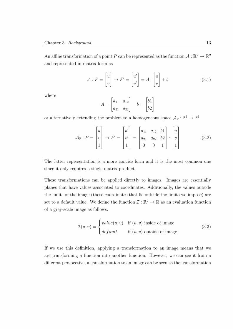
An affine transformation of a point P can be represented as the functionA : R2 → R2
and represented in matrix form as
A : P =
[u
v
]→ P ′ =
[u′
v′
]= A ·
[u
v
]+ b (3.1)
where
A =
[a11 a12
a21 a22
]b =
[b1
b2
]or alternatively extending the problem to a homogeneous space AP : P2 → P2
AP : P =
u
v
1
→ P ′ =
u′
v′
1
=
a11 a12 b1
a21 a22 b2
0 0 1
·u
v
1
(3.2)
The latter representation is a more concise form and it is the most common one
since it only requires a single matrix product.
These transformations can be applied directly to images. Images are essentially
planes that have values associated to coordinates. Additionally, the values outside
the limits of the image (those coordinates that lie outside the limits we impose) are
set to a default value. We define the function I : R2 → R as an evaluation function
of a grey-scale image as follows.
I(u, v) =
value(u, v) if (u, v) inside of image
default if (u, v) outside of image(3.3)
If we use this definition, applying a transformation to an image means that we
are transforming a function into another function. However, we can see it from a
different perspective, a transformation to an image can be seen as the transformation

Chapter 3. Background 14
of the sample points that are going to be substituted in the formula from above.
There is no need to express a function-to-function transformation. For instance, in
this alternative, if we wanted to move the image to the left, we would need to move
the sample points’ coordinates to the right as illustrated similarly in figure 3.1.
(a) Sample grid before transforma-tion
(b) Sample grid after moving imageto the left
Figure 3.1: Classic cameraman image with sample points showing duality.
In the definition 3.3, we have not described how does the function value behave. In
practice, images do not have infinite resolution and it is common to take samples
from the image that do not match an exact coordinate with an existing value in the
image. Thus, if we have a discrete image, we will have a discrete function I. Since
we may want to be able to sample non-discrete points that do not exactly match,
we need to convert I into a non-discrete function. We may want, for example, to
retrieve a value that is close to the values of the surrounding points. We can actually
choose between a continuous function or a function with discontinuities such as in
nearest-neighbor filtered images. Throughout the years, several techniques have
been developed, such as linear interpolation between values of neighboring points.
There are lots of ways to deal with this problem and choosing one method or another
depends on the interest of the user.

Chapter 3. Background 15
3.1.2 3D transformations and pinhole camera model
In the cases presented in this document, we are going to concentrate mostly on 3D
scenes and objects since that is what RGB-D cameras information give us about the
environment. Therefore, we use the following assumptions:
• The target is a 3D rigid object represented as a set of sampled points that relate
a position in space with data retrieved by the camera. These are also known
as point clouds. Since the object is not deformable, a subset of points cannot
move relatively to another subset of points, all points must move together as
a whole set using the same transformation.
• The motion model has to be compatible with these 3D point clouds, thus, our
motion model is a 3D rigid body transformation.
• For the virtual camera, we are going to use the pinhole-camera model [34].
The motion model describes in this case how every single point of the point cloud
is going to behave between two different frames or iterations separately. The 3D
rigid body transformation can be applied separately to every single point as long as
each point has at least the coordinates in the form (X, Y, Z) for a three dimensional
space. Apart from the location data, point clouds can have additional data. In our
case, that data can be intensity image values or color values. If we assume that
we can separate the position data from the additional data in each point, we can
perform the transformations using matrix algebra using homogeneous coordinates.
The function T6dof3D : P3 → P3 is defined as
T6dof3D : P → PT = T6dof3D · P (3.4)

Chapter 3. Background 16
where
PT =
XT
YT
ZT
1
T6dof3D =
[R ~t
0 1
]P =
X
Y
Z
1
The matrix T6dof3D is the 3D rigid body transformation matrix of six degrees of
freedom which are the three Euler angles expressed as the rotation matrix R and the
three translation degrees of freedom in the three dimensional space. As the reader
may note, points P and PT have the said three coordinates and also have the forth
coordinate set to 1. This forth coordinate is necessary to perform our transformation
correctly in an affine manner and is also present in the transformation matrix. The
expression of a location in four coordinates in this way as homogeneous coordinates.
It is assumed that the reader is familiar with this concept and it is not explained
any further.
The function that describes this rotation is R : R3 → R3. The associated matrix
is the parametric rotation matrix R and is obtained using a product of rotation
matrices in each axis as follows.
R ≡ R(α, β, γ) = RZ(γ) ·RY (β) ·RX(α) (3.5)
where
RX(α) =
1 0 0
0 cosα − sinα
0 sinα cosα
RY (β) =
cos β 0 sin β
0 1 0
− sin β 0 cos β
RZ(γ) =
cos γ − sin γ 0
sin γ cos γ 0
0 0 1

Chapter 3. Background 17
The parametric translation vector can be expressed as the transposed vector ~t ≡~t(t1, t1, t3) = [t1 t2 t3]T .
Henceforth, the transformation can be seen as a matrix that is generated using
those six parameters and the formula of T6dof3D at the definition 3.4. The result is a
parametric matrix of the form T6dof3D(α, β, γ, t1, t1, t3).
Finally, we only need to specify the camera model. We are going to use the classic
pinhole-camera model which can be expressed as the product of two parametric
matrices, the camera intrinsics matrix K and the camera extrinsics matrix C. These
two matrices are used in conjunction with the transformation matrix to generate
the final transformation. The transformation of K and C together is known as
perspective projection and can be noted as p : P3 → P2.
p : PC → PS =[K 0
]·
PC︷ ︸︸ ︷C · PT (3.6)
where
PS =
λj
λi
λ
K(f, ku, kv, s, i0, j0) =
fku s j0
0 fkv i0
0 0 1
PC =
XC
YC
ZC
1
C =
[RC
~tC
0 1
]
The matrix RC and the vertical vector tC are also a rotation matrix of three degrees
of freedom (three angles) and a translation vector of three degrees of freedom respec-
tively, of course, both are also parametric. C is a six degrees of freedom matrix but,
unlike T6dof3D, this one represents the transformation of the point cloud from world
coordinates into camera coordinates. λ represents the depth value of the projected

Chapter 3. Background 18
point and it is distinguished in such a way because all values must be divided by it
as the last part of the projection procedure, this is usually referred to as perspective
divide.
In the pinhole-camera model, we assume that the camera is aligned with the Z axis
and that it is facing towards +Z. Screen borders are also aligned to the XY axis.
Usually, if we express the resulting image as a matrix, the first axis (axis of the
is), would be aligned to +Y while the second axis (axis of the js) would be aligned
to +X. Therefore, when we develop the matrix C, we must take this details into
account so that the camera is facing towards the parts of the scene that we are
interested in.
3.2 Direct methods
Before any definition is given, some concepts are going to be settled. In the image
registration context, we will refer to the target image as template or reference image
whereas the image that we iteratively transform until we find a match with the
template is referred as the input image.
Direct methods attempt to transform the input image into the template image so
that we can compute an estimation of the transformation that converts one image
into the other image. This can be used for various purposes. In our case, we want to
know the motion of our target. In particular, in the three dimensional case, we are
going to use point clouds and we want to know the motion of the entire point cloud
assuming that the camera is fixed or, alternatively, treat the point cloud as if it was
fixed and know the motion of our camera. This double and relative interpretation
of the problem is going to be referred in this document as duality.
Before the description of the main algorithms that are used in this document, some
requirements and more definitions must be introduced. The notation employed in

Chapter 3. Background 19
the development of the explanations in this section is going to be similar to the
notation from the thesis [1] and the related article [35].
First, a clear definition of our image registration problem is provided. We start with a
couple of intuitive counterexamples. In these problems we do not change the original
colors of the input image or those of the template image. We will also preserve the
structure of the neighborhoods between transformed points in the original images.
This means that the corresponding points match if the colors match. Formally, the
Brightness Constancy Assumption is introduced as the main requirement in image
registration. The BCA is defined as
I(f(x, µ), t) = T (x),∀x ∈ V ⊂ D (3.7)
where I(x′, t) is the input image evaluated at the point x′ = f(x, µ) ∈ V ′ ⊂ D and
at time t, f(x, µ) : D × Rp → D is the warping function (transformation function)
which applies the warp described by µ with p parameters to the initial point x and
T (x) is the template image evaluated at x. V and V ′ are arbitrary sets of points
that must be within the function domain D.
In general, all direct methods in image registration require a series of common steps.
They require dissimilarity measure, dissimilarity linearization, search direction com-
putation and parameter and image update steps. All of them also perform a con-
vergence check so that the algorithm is stopped when certain criteria is met. There
are multiple ways to define such criteria, however, in this document, only the one
that is chosen for the experiments is presented.
The convergence criteria or, to be more precise, the halting criterion is a fixed
threshold for the step increment (δps in the following formulas) norm. If this norm
is greater than a threshold, the algorithm is stopped and the test is considered
as divergent. If the norm is smaller than another threshold, the algorithm is also

Chapter 3. Background 20
stopped and the test is considered as convergent. Additionally if a fixed amount of
iterations is surpassed, the algorithm is stopped but no conclusions are derived.
The algorithms that have been chosen to solve the image registration problem are the
Lucas-Kanade algorithm [9] and the Inverse Compositional algorithm [13, 14]. We
will refer to them therefore as LK and IC respectively for the rest of the document.
3.2.1 Lucas-Kanade
The first algorithm that is going to be described here is the Lucas-Kanade algo-
rithm. It is a forward additive direct method and it is based on the Gauss-Newton
optimization scheme. The dissimilarity measure that is used in this algorithm is the
squared residual. The residual is the dissimilarity between the input image and the
template image and is defined as r(µ) ≡ T (x)−I(f(x, µ), t+1)1. The corresponding
dissimilarity linearization would then be
r(µ+ δµ) ' L(δµ) ≡ r(µ) + r′(µ) δµ = r(µ) + J(µ) δµ (3.8)
where J(µ) ≡ −∂I(f(x, µ), t+ 1)
∂µ
∣∣∣∣µ=µ
is known as the Jacobian of the warped image
I(f(x, µ), t+1) evaluated at µ. The parameter increment δµ is used in every iteration
to update the parameters additively as follows µ′ = µ+δµ. This linearization follows
the Newton minimization method and as such, to perform the linearization, a first
order Taylor series is required to locally estimate the parameters of the warp at
each step. In the Newton minimization method we would find xn in 0 = f(xn−1) +
f ′(xn−1) (xn − xn−1). In this case, we find δµ in our dissimilarity measure which is
1r(µ) depends also on other parameters such as x or t but these are initialized once and areregarded as constants throughout the whole algorithm so there is no need to parameterize those.
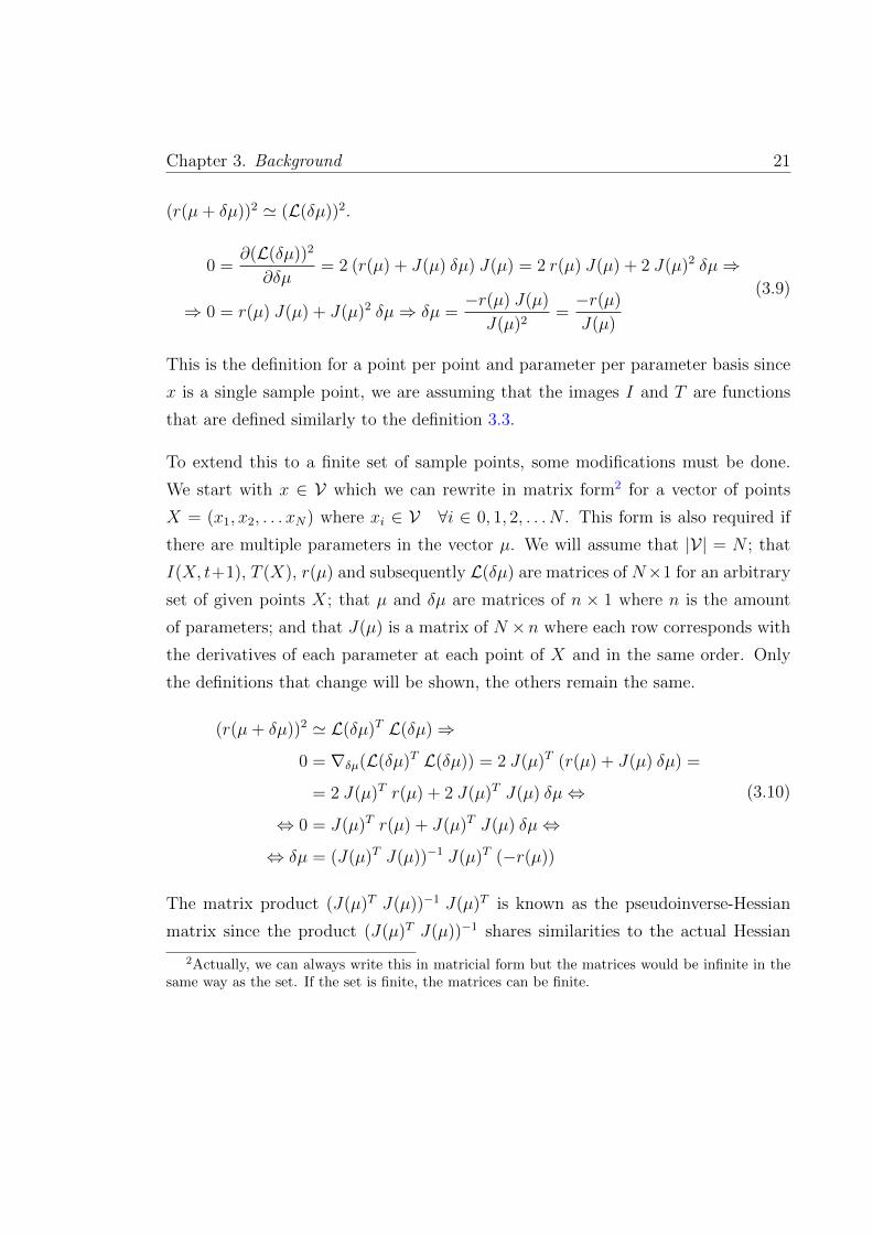
Chapter 3. Background 21
(r(µ+ δµ))2 ' (L(δµ))2.
0 =∂(L(δµ))2
∂δµ= 2 (r(µ) + J(µ) δµ) J(µ) = 2 r(µ) J(µ) + 2 J(µ)2 δµ⇒
⇒ 0 = r(µ) J(µ) + J(µ)2 δµ⇒ δµ =−r(µ) J(µ)
J(µ)2=−r(µ)
J(µ)
(3.9)
This is the definition for a point per point and parameter per parameter basis since
x is a single sample point, we are assuming that the images I and T are functions
that are defined similarly to the definition 3.3.
To extend this to a finite set of sample points, some modifications must be done.
We start with x ∈ V which we can rewrite in matrix form2 for a vector of points
X = (x1, x2, . . . xN) where xi ∈ V ∀i ∈ 0, 1, 2, . . . N . This form is also required if
there are multiple parameters in the vector µ. We will assume that |V| = N ; that
I(X, t+1), T (X), r(µ) and subsequently L(δµ) are matrices of N×1 for an arbitrary
set of given points X; that µ and δµ are matrices of n × 1 where n is the amount
of parameters; and that J(µ) is a matrix of N ×n where each row corresponds with
the derivatives of each parameter at each point of X and in the same order. Only
the definitions that change will be shown, the others remain the same.
(r(µ+ δµ))2 ' L(δµ)T L(δµ)⇒
0 = ∇δµ(L(δµ)T L(δµ)) = 2 J(µ)T (r(µ) + J(µ) δµ) =
= 2 J(µ)T r(µ) + 2 J(µ)T J(µ) δµ⇔
⇔ 0 = J(µ)T r(µ) + J(µ)T J(µ) δµ⇔
⇔ δµ = (J(µ)T J(µ))−1 J(µ)T (−r(µ))
(3.10)
The matrix product (J(µ)T J(µ))−1 J(µ)T is known as the pseudoinverse-Hessian
matrix since the product (J(µ)T J(µ))−1 shares similarities to the actual Hessian
2Actually, we can always write this in matricial form but the matrices would be infinite in thesame way as the set. If the set is finite, the matrices can be finite.

Chapter 3. Background 22
matrix (second order derivative in matrix form). The explanation can be found in
the appendix section of the article [14]. The algorithm can be summarized in the
steps shown in the algorithm figure 3.1.
Algorithm 3.1: LK algorithm summary
On-line: Let µi = µ0 be the parameter initializationwhile halting criteria not satisfied do
Residual calculation at r(µi)Jacobian calculation at J(µi)Calculate search direction using either 3.9 or 3.10Update parameters additively using µi+1 = µi + δµ
end
3.2.2 Inverse Compositional
The Inverse Compositional method has almost the same core steps but there are
several important differences. The IC is inverse, which means that the search of
parameters is performed backwards, so instead of defining the Jacobian in terms of
the input image, it is defined in terms of the template image. The IC is composi-
tional, which means that instead of performing the parameter update in an additive
fashion, it composes the resulting warps (function composition). This makes the IC
an efficient algorithm in terms of performance because the Jacobian can be calcu-
lated only once as the template image does not change between different iterations.
The algorithm also uses the squared residual as the dissimilarity measure as in LK
(3.2.1). The other differences are now presented formally.
In IC the residual has to be defined differently since this algorithm uses an inverse
strategy, r(µ) ≡ T (f(x, µ))− I(f(x, µaccum), t+ 1) where µaccum is the accumulated
warp and therefore, it is a transformation and not a vector of parameters or a pa-
rameter. Since this is an inverse approach, all the local minimizations are performed
Chapter 3. Background 23
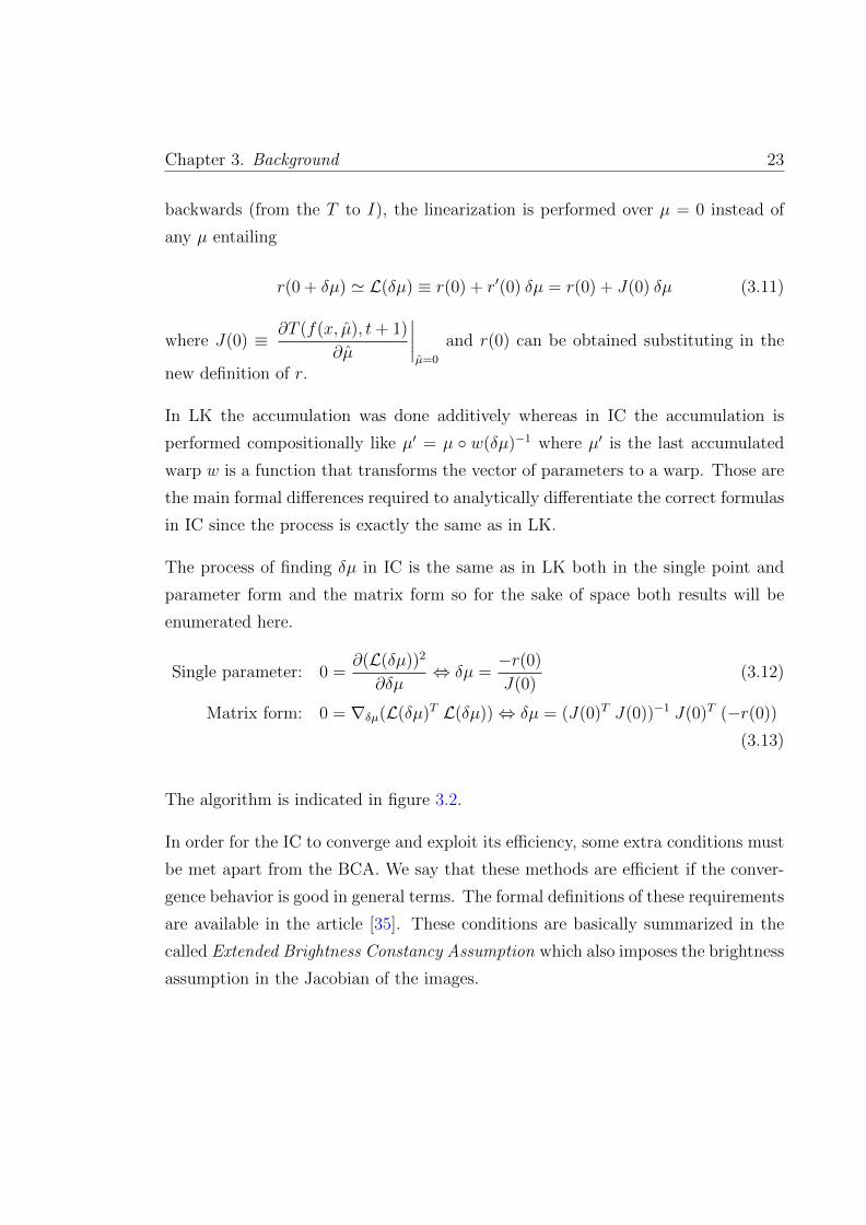
backwards (from the T to I), the linearization is performed over µ = 0 instead of
any µ entailing
r(0 + δµ) ' L(δµ) ≡ r(0) + r′(0) δµ = r(0) + J(0) δµ (3.11)
where J(0) ≡ ∂T (f(x, µ), t+ 1)
∂µ
∣∣∣∣µ=0
and r(0) can be obtained substituting in the
new definition of r.
In LK the accumulation was done additively whereas in IC the accumulation is
performed compositionally like µ′ = µ ◦ w(δµ)−1 where µ′ is the last accumulated
warp w is a function that transforms the vector of parameters to a warp. Those are
the main formal differences required to analytically differentiate the correct formulas
in IC since the process is exactly the same as in LK.
The process of finding δµ in IC is the same as in LK both in the single point and
parameter form and the matrix form so for the sake of space both results will be
enumerated here.
Single parameter: 0 =∂(L(δµ))2
∂δµ⇔ δµ =
−r(0)
J(0)(3.12)
Matrix form: 0 = ∇δµ(L(δµ)T L(δµ))⇔ δµ = (J(0)T J(0))−1 J(0)T (−r(0))
(3.13)
The algorithm is indicated in figure 3.2.
In order for the IC to converge and exploit its efficiency, some extra conditions must
be met apart from the BCA. We say that these methods are efficient if the conver-
gence behavior is good in general terms. The formal definitions of these requirements
are available in the article [35]. These conditions are basically summarized in the
called Extended Brightness Constancy Assumption which also imposes the brightness
assumption in the Jacobian of the images.

Chapter 3. Background 24
Algorithm 3.2: IC algorithm summary
Off-line: Jacobian calculation at J(0)On-line: Let µi = w(µ0) be the warp initializationwhile halting criteria not satisfied do
Residual calculation at r(µi)Calculate search direction using either 3.12 or 3.13Update warp compositionally using µi+1 = µi ◦ w(δµ)−1
end
Formally these requirements can be expressed as
BCA: I(f(X,µ), t) = T (X) (formula 3.7 and X = V)
EBCA: BCA and X = g(X ′, φ0 + ∆φ)⇒
⇒ I(f(g(X ′, φ0 + ∆φ)) = T (g(X ′, φ0 + ∆φ))
(3.14)
where X ∈ D and X ′ ∈ D are sets of points and f and g are warps and φ0 is a
vector of parameters and ∆φ is a small increment of this vector.
The EBCA implies that the brightness constancy must be also maintained over
a composition of warps (requirement 1) with a small increment (requirement 2)
which is equivalent to saying that it has to be maintained in the Jacobian of the
input images and the template image. In the original article, these requirements
are referred to as parameter equivalence and parameter independence respectively.
If the reader seeks further understanding of the theory behind the EBCA and its
implications and the results in various experiments, all the information is carefully
presented in [35]. The theory of the EBCA is in section 4 and the experiments are
in section 5.

Chapter 3. Background 25
3.2.3 Other notable mentions
There are other important variants of direct methods that are worth mentioning in
the topic. These techniques are not going to be explained in detail since they are
not going to be used in the rest of the document unlike LK or IC and they are well
explained in their respective articles.
The first approach worth mentioning is Hager-Belhumeur [10] algorithm which is a
variant of LK. It is an additive approach that attempts to reduce the computational
costs of it. The latter performs many computations in every iteration since it has
to recalculate the Jacobian at every step (see the step calculation formula of δµ at
3.10). Hager-Belhumeur reduces the computational time using the derivatives of
the template image in the gradient calculation and performing a factorization of the
Jacobian matrix so that at least one part can be computed off-line (this part also
includes the gradient image of the template).
The second and last approach is the Forward-Compositional [11, 12] algorithm which
is a compositional algorithm. The procedure is very similar to the IC as well as
the resulting formulas required for each step. The main difference is that all the
calculations of the Jacobian are made over the input images instead of the template
image. This implies that the Forward-Compositional algorithm is far slower than
its inverse since it has to recalculate the Jacobian at every iteration as the input
images also change between iterations.
3.2.4 Additional improvements
Apart from these algorithms and their variants, there are several improvements that
can be applied to them depending on the case. These improvements are changes
to parts of the previous algorithms that attempt to address certain problems these
algorithms present in certain cases.

Chapter 3. Background 26
For example, we may want to use an algorithm such as LK for its compatibility
reasons but we may also need computation performance offered by algorithms such
as IC. In case we want to improve the performance of any algorithm, pixel selection
techniques can serve that purpose. And if we want to improve the convergence, we
may consider using coarse-to-fine schemes.
The objective in pixel selection is to reduce the amount of pixels to be processed
from the original images. This can improve two aspects of the main algorithm.
As mentioned before, pixel selection can improve performance and this is under-
standable since the matrices that we are going to work with after pixel selection are
obviously going to be of smaller or equal size as the original. But it can also have
another desirable effect over the algorithm. If pixel selection is able to determine
which pixels are not appropriate to achieve convergence in the algorithm because
these pixels are either uninformative in comparison to others or they contradict the
gradient given by other pixels (nullifying the final gradient result), these pixels can
be removed to aid the main algorithm in the residual minimization. So the benefits
provided by this technique may be twofold.
In coarse-to-fine selection schemes the strategy is to accelerate convergence reducing
the resolution and also smoothing the image since it is known that smoother images
have better convergence. This is achieved using what is called a pyramid [36] of
images where each layer of the pyramid is a lower-resolution version of the original
images with a low-pass filter such as the Gaussian filter. The minimization process
starts at the lowest resolution until convergence is achieved. Then the algorithm
changes the images to others of higher resolution (next layer) and starts to iterate
using the direct image alignment algorithm again at the previous parameter results
(change of the algorithm initialization). This process is repeated until all the layers
of the pyramid have been used and, in theory, a greater degree of convergence is
achieved. In the literature, the algorithm is usually referred as “multi-resolution”

Chapter 3. Background 27
as well. These are several references were the last two algorithms is employed [23–
29, 37]. An example of coarse-to-fine scheme applied on a single image, see figure
3.2.
Figure 3.2: Several layers of the pyramid in a coarse-to-fine scheme.
Other strategies may not attempt to reduce the amount of pixels directly but instead
they attempt to improve the robustness and accuracy of the algorithm in cases that
certain parts of the images are not reliable for image registration. This is referred to
as robust estimation. Those parts are usually considered outliers for the algorithm
since they are those that decrease reduce convergence. This is actually very similar
to pixel selection but it does not reduce the amount of pixels in images. This
technique uses the residual as the guide to know how much do we have to rely
on each pixel’s information. This reliance is provided as a diagonal matrix that is
calculated directly from the residual and a chosen robust M-estimator [26, 38] and,
following our previous notation, it can be formalized as
O(x) = ρ
(∑x∈V
r(x)
)(3.15)

Chapter 3. Background 28
where ρ is our estimation function and O is the final estimated value for each point
x. Depending on the way we formalized the direct method, we may obtain different
formulas for each step and different precomputations. For the sake of clarity, we show
how is this applied to LK. If we take the resulting parameter update formula 3.10,
we can derive the following formula (based on [26]) with the robustness estimation
capability
δµ = (D J)+ D (−r(µ)) (3.16)
where (D J)+ is the pseudo-inverse matrix of D · J . This diagonal matrix serves
as a series of weights for each pixel so that the more reliable a pixel is, the higher
the weight is and, consequently, the more it influences in the final result of the
minimization step. In the previous formula it can be seen that the matrix product
and the pseudo-inverse must be calculated each iteration and, henceforth, it is not
beneficial for algorithms such as the IC because the reason behind their existence is
the attempt to reduce the amount of calculations.
3.3 RGB-D cameras
In this section, a brief introduction to the various RGB-D cameras is presented to
give the reader a brief notion of how are these images usually generated. We can
divide current depth sensing techniques into three different categories [39]:
• Interferometry: based on the measurements made over the amount of inter-
ference between monochromatic waves. This technique is very precise in short
distances ranging from micrometers to centimeters.
• Triangulation: these try to measure depth using the virtual triangle that is
formed between the lines of sight of an optical system and a point in the scene.

Chapter 3. Background 29
• Time of Flight: these perform measurements of the time-of-flight of signals
emitted from the source of the camera to a point in the scene that subsequently
collides and bounces back to the camera receiver. Typically, the most popular
techniques in ToF are those based on Continuous Wave Modulation and those
based on Photometric Mixer Device ToF. In these cases, the phase shift dif-
ference between the emitted and received signal is measured to calculate the
distance (depth).
In triangulation, there are essentially two main trends depending on how is the
triangulation performed. The triangulation can be performed actively or passively.
When we perform passive triangulation, our optical system is made of several (at
least two) cameras that serve as stereo vision. The procedure to perform triangula-
tion is passive since correspondences of points in the scene seen from various cameras
have to be found. Once a match is found for every pixel in the image obtained from
each camera (or at least, some pixels), triangulation can be performed unless those
cameras are aligned with a given point in the images. Thus, the triangle must have
an area different from zero.
If active triangulation is performed, the optical system has light sources instead
of various cameras (only a single camera is needed). This greatly improves the
matching task since each point can be emitted from the light source in the desired
direction. The camera must find how is the scene modifying the emitted ray in order
to calculate the distance via triangulation. For a single distance measurement, this
is trivial since there is only going to be one point of emitted light and the camera
is going to perceive the reflected light at the expected position or relatively close
to it. However, if several distances are meant to be calculated, for instance, the
distance of each pixel in the camera, it is necessary to perform one calculation at a
time. With the appearance of Kinect sensors and its derivative, this is no longer a
problem. The Kinect sensor is an example of active triangulation using an emitted

Chapter 3. Background 30
light-pattern that is known a priori and the deformations of this pattern provide the
depth information via triangulation. The only drawback is that the pattern cannot
provide good accuracy in camera space unless greater camera resolution is provided
to the system. This would require a faster processor and it would be more expensive
not only because of the processor but also because of the greater camera resolution
and light emitter resolution. The instructions to setup a Kinect sensor are provided
in the appendix A.

Chapter 4
Methodology
This chapter serves as a farther explanation of the implementation details of LK and
IC, especially those related to the Jacobian calculation and the procedure to adapt
LK and IC to RGB-D based images.
4.1 The unidimensional case
To start understanding the behavior of any sort of direct method (in general, all
those derived from LK, see 3.2.1), one-dimensional examples may serve better for
introductory purposes.
To simplify our examples and assure convergence, the BCA (see definition 3.7) must
be satisfied. In one-dimensional examples, any simple continuous function can satisfy
it. These simple continuous functions will serve as the equivalent to the template
and input images that were explained in chapter 3. In the following examples, the
function g will serve as the equivalent of the template image (in this case is the
target shape of our function) and f will be the equivalent of the input image which
31

Chapter 3. Methodology 32
in principle is the same as g (if it was not, it would not satisfy the BCA) but
it is affected by an offset transformation. The transformation must satisfy BCA
conditions as well.
For example, we choose a simple unidimensional continuous function such as a Gaus-
sian function defined as G(x) =1√
2 π σ2exp
(−(x− µ)2
2 σ2
)and we perform a simple
transformation. The simple transformation will be an offset (also known as transla-
tion or commonly as a shift) in parameter µ since it establishes where is the median
in the Gaussian distribution function and, therefore, it shifts all the function in the
x variable axis.
To illustrate this, the reader can see figure 4.1 which shows two Gaussian functions.
Function g is centered at µ = 1 while function f is centered at µ = 0. The surfaces
associated to the residuals (see 3.2 to understand what the residual is) and their
derivatives with different parameters are also provided in figure 4.2. The derivatives
are, of course, what we have been calling the Jacobian (see 3.2 as well if needed).
Figure 4.1: Function g is centered at 1 while function f is centered at 0.

Chapter 3. Methodology 33
(a) Residual (b) Residual derivative
(c) Residual second derivative givenjust to understand the function’s be-
havior
Figure 4.2: Residual and its derivatives depending on the parameter µ which isrenamed in the axis as p
The residual surfaces in 4.2 show that the residual r changes as the parameter µ
changes. In the first surface, it can be seen that the difference between f and g
is smaller as the µ of f gets closer to the µ of g. This is especially notable when
both f and g match each other and the surface is flat. This happens when µ = 1 as
expected.
If we perform a Newton optimisation we can iterate over f(x, µ) until µ ≈ 1. The
Newton method applies to a single starting point rather than a set or vector of points
and in our case the minimization is done over a set of sampled points (in figure 4.1

Chapter 3. Methodology 34
we are working with the (-4,4) range of values as the graph shows). We need then
the matrix form to be able to work with this set of points which is equivalent to using
the Gauss-Newton method as seen in section 3.2.1. In this example, we perform this
optimisation step over µ using the LK algorithm (see 3.1).
(a) Residual at µ = 0 (b) First product at µ = 0 withoutsign
(c) Second product (pseudo-inverse) at µ = 0
Figure 4.3: First iteration of the optimisation
In each iteration, the graphs show the product to obtain each increment δµ divided
into two parts. The first part of the product in equation 3.10 is (−J(µ)T r(µ)) where
J and r are sampled at every point of the set. With a single parameter, this can
be graphically illustrated as the area under the curve of these products (colored in
red in figure 4.3) if we had an infinite amount of sample points. In these examples,
it is not exactly the area but for the sake of clarity, the area will be used to show

Chapter 3. Methodology 35
the behavior of the LK algorithm since it is more intuitive graphically1. The second
product is the one related to the pseudo-inverse matrix (J(µ)T J(µ))−1. This one
can also be regarded as the area under the curve but with the inverse effect on δµ.
This implies that for the first part, the larger the area under the curve, the larger
the value that will result in δµ for the following iteration and with opposite sign
because of the minus. Note that this area can be positive or negative. However, the
second part has the inverse behavior, meaning that the larger the area under the
curve, the smaller δµ will be. Also note that this area cannot ever be negative since
the square of any number or in particular, the square of the Jacobian, cannot be
negative by the definition of a square operation in a matrix.
The first iteration (figure 4.3) leads clearly towards a greater value of µ because of
the larger negative area against the positive area of the first product, then the sign
is inverted leading to a positive value. The second product is large enough to make
the final value to be relatively lower. This is a desired effect since the closer we are
to the result, the smaller we want the steps to be.
The following two iterations (figures 4.4 and 4.5) show that there is a clear con-
vergence and in the last iteration the area of the first product is almost invisible.
The algorithm converges with µ = 0.999999994936 just using a halting criterion of
a minimum norm of 0.1 per increment.
Since our direct methods rely on local optimisations and, consequently, on the initial-
ization parameters, these are essential for the convergence of the algorithm. Because
of their nature, these algorithms can converge to local optima and this is unavoidable
if the source of data is ambiguous. In our unidimensional example we can create a
f function that instead one Gaussian distribution, it has two Gaussian distributions
sufficiently separated. If the initialization is done in such a way that one of the
1Actually it is just the height at each sampled point rather than the area. It would be the areaif there was an infinite amount of points.

Chapter 3. Methodology 36
(a) Residual at µ = 0.779 (b) First product at µ = 0.779 with-out sign
(c) Second product (pseudo-inverse) at µ = 0.779
Figure 4.4: Second iteration of the optimisation
Gaussian distributions in f matches the other Gaussian distribution in g but that
does not happen for the other pair of Gaussian peaks, the wrong peak is matched
and convergence will most likely be reached immediately towards the local optima.
But this is not the only drawback that we can find in locally-based algorithms. Con-
vergence can also be impossible to achieve if f and g are not sufficiently close even
without any sort of global ambiguities. To show this, another example is proposed
that is directly derived from the previous one.
The example in figure 4.6 shows a case where, according to the algorithm, conver-
gence is achieved in the first iteration using the 0.1 norm threshold as we did before.

Chapter 3. Methodology 37
(a) Residual at µ = 0.997 (b) First product at µ = 0.997 with-out sign
(c) Second product (pseudo-inverse) at µ = 0.997
Figure 4.5: Third iteration of the optimisation
This shows that, in this variant, the algorithm cannot decide how to choose the
next parameter increment since the data is not good enough. If the threshold is
changed from 0.1 to 0.001, the algorithm keeps slowly iterating until it gets to the
destination due to the fact that Gaussian distributions are always above zero and
their derivative is never zero in R. If we use a different function were the derivatives
and the residual do not aid at all, convergence will be impossible regardless of the

Chapter 3. Methodology 38
(a) f and g at µ = −4 (b) First product at µ = −4 with-out sign
(c) Second product (pseudo-inverse) at µ = −4a
aIn this graph there is a representa-tion error due to Matplotlib’s filling al-gorithm, the area should be filled fromthe axis but they use the enclosed poly-gon instead.
Figure 4.6: Example of slow convergence
chosen threshold. Functions like the following can be used to cause such problems
f(x, µ) =
0 if x ∈ (−∞,−1 + µ]
cos(π(x− µ))
2+ 0.5 if x ∈ (−1 + µ, 1 + µ]
0 if x ∈ (1 + µ,∞)
(4.1)

Chapter 3. Methodology 39
This case is also illustrated in another figure 4.7. Convergence is eventually achieved
in the implementation of this example using a very low threshold, but this is due to
the lack of samples (50 samples in the x axis for all these examples) which provides
some noise that can help in the convergence eventually though it is unlikely. And
the more samples are used for this test, the worse the convergence is2.
(a) f and g at µ = −2 (b) First product at µ = −2 with-out sign
(c) Second product (pseudo-inverse) at µ = −2
Figure 4.7: Example of no convergence
Hopefully, these simple examples illustrate how LK works for a single parameter
(unidimensional optimisation). From now on, any arbitrary amount of parameters
2This has been also tested using 1000 samples and the convergence is several times lower thanbefore. This has not been chosen at first so that these strange cases could arise so that a betterobservation is made.

Chapter 3. Methodology 40
will be used in the examples and reasoning. Next sections will not be as rich in
detailed examples since it will be assumed that the basic understanding process has
already been completed by the reader after reading these experiments.
4.2 Implementation details
This section presents some details of the implementation that have been used through-
out this document to perform the experiments. If no comments are made about a
certain detail of LK or IC or any definition provided in chapter 3, it means that the
exact definitions available in that chapter are used. Advantages and disadvantages
of each implementation choice are also discussed in this section.
4.2.1 Jacobian calculation
Probably, the most important choice while implementing either LK or IC is how to
calculate the Jacobian matrix. The Jacobian matrix is the core of both algorithms
and also of other variants like those presented in section 3.2.3 or those cited in the
literature review at 2.4.
The Jacobian matrix influences in the final increment value of each iteration in a
very meaningful way since it affects the pseudo-inverse as we have seen in previous
section 4.1 and also in the original formulas from sections 3.2.1 and 3.2.2. The
Jacobian matrix can be calculated in many different ways and the technique used is
entirely the implementer’s choice, yet, it is crucial that the chosen implementation
is equivalent to the definitions established in those sections. If the definitions are
not met, it is likely that the algorithms will not perform well in practice.
Chapter 3. Methodology 41
In this document, two possible implementations (and some other hybrids) for the
Jacobian in LK and in IC are discussed: the analytic Jacobian and the numeric
Jacobian.
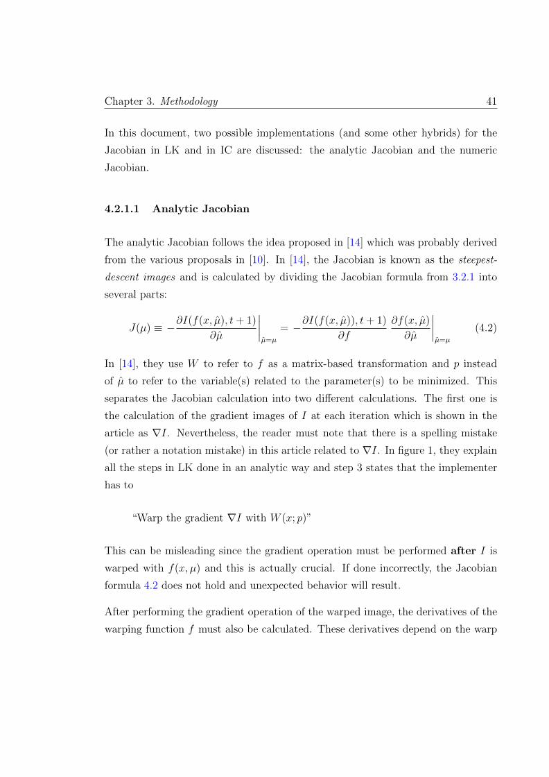
4.2.1.1 Analytic Jacobian
The analytic Jacobian follows the idea proposed in [14] which was probably derived
from the various proposals in [10]. In [14], the Jacobian is known as the steepest-
descent images and is calculated by dividing the Jacobian formula from 3.2.1 into
several parts:
J(µ) ≡ −∂I(f(x, µ), t+ 1)
∂µ
∣∣∣∣µ=µ
= −∂I(f(x, µ)), t+ 1)
∂f
∂f(x, µ)
∂µ
∣∣∣∣µ=µ
(4.2)
In [14], they use W to refer to f as a matrix-based transformation and p instead
of µ to refer to the variable(s) related to the parameter(s) to be minimized. This
separates the Jacobian calculation into two different calculations. The first one is
the calculation of the gradient images of I at each iteration which is shown in the
article as ∇I. Nevertheless, the reader must note that there is a spelling mistake
(or rather a notation mistake) in this article related to ∇I. In figure 1, they explain
all the steps in LK done in an analytic way and step 3 states that the implementer
has to
“Warp the gradient ∇I with W (x; p)”
This can be misleading since the gradient operation must be performed after I is
warped with f(x, µ) and this is actually crucial. If done incorrectly, the Jacobian
formula 4.2 does not hold and unexpected behavior will result.
After performing the gradient operation of the warped image, the derivatives of the
warping function f must also be calculated. These derivatives depend on the warp

Chapter 3. Methodology 42
that is going to be used during the process. For example, the derivatives of an affine
warp in 2D and in matrix form are
∂f(~x, µ)
∂µ=
([x 0 y 0 1 0
0 x 0 y 0 1
](x, y)
)· ~x (4.3)
as shown in [14]. This article offers other derivatives for other transformations as
well.
In the IC algorithm, the same can be done using the formulas discussed in section
3.2.2.
J(0) ≡ ∂T (f(x, µ), t+ 1)
∂µ
∣∣∣∣µ=0
=∂T (f(x, µ), t+ 1)
∂f
∂f(x, µ)
∂µ
∣∣∣∣µ=0
(4.4)
The calculation process in practice is shown in figure 4.9 where gx and gy are the
respective gradients in both axis and Jxp1 and Jyp1 are the analytic derivatives of
the warping function (in Jxp1 black is -1, grey is 0 and white is 1). The gradients
and the Jacobians are multiplied per-pixel in the same axis where the result of each
product are the two images on the right. These images are added per-pixel giving
the final Jacobian which is the one that appears with the label Jp1.
Figure 4.8: Texture image used in figure 4.9 (4 Gaussian distributions in 2D).

Chapter 3. Methodology 43
Figure 4.9: Analytic Jacobian in one parameter generated in various steps. p1is the actual Jacobian.
Both LK and IC require the calculation of the gradient images∇I and the calculation
of the warp derivatives∂f(x, µ)
∂µ. The gradient images have to be calculated over
discrete sets of sample points since after warping (and also before) the transformed
image is also made of pixels which by nature are discrete and finite (this has already
been discussed in section 3.1.1)). To perform these derivatives images must be
treated as if they were continuous functions, so a special procedure is required.
There are various ways to calculate this:
• Derivative definition: using the general definition of derivation3, we can
calculate the derivatives per pixel in one axis. This can be applied performing
3The definition that is referred to is f ′(x) =f(x+ α)− f(x− α)
2 α

Chapter 3. Methodology 44
a horizontal or vertical convolution with a kernel K = [−1 0 1]T or K =
[−1 1]T . This definition is suitable in general but it does not take into account
neighboring pixels others than those aligned with the current pixel in the
current axis.
• Sobel filter: the Sobel filter can be applied to create gradient images. This
filter does take into account all 8 neighboring pixels of the current pixel since
it performs a convolution with a kernel of 3× 3 which is usually of the form4
KSobelX =
−1 0 1
−2 0 2
−1 0 1
(4.5)
For the vertical version, use the transpose matrix KTSobelX.
• Scharr filter: this filter is similar to the Sobel filter since it is also based on
a convolution of a 3× 3 kernel. This kernel is supposed to yield better results
since it resembles more a Gaussian filter.
KScharrX =
−3 0 3
−10 0 10
−3 0 3
(4.6)
The last two techniques are more accurate because they mimic a continuous function
where each pixel is a Gaussian distribution with a certain maximum value. It can be
imagined as a surface where the heights at each point are the image values and each
sampled point is a Gaussian distribution with the median centered at that point.
4This kernel and the Scharr kernel are provided in OpenCV and this is the URL where the ma-trices have been taken from http://docs.opencv.org/modules/imgproc/doc/filtering.html?
#sobel (July 2015)

Chapter 3. Methodology 45
All of these variants provide the gradients over a single axis, so in order to calculate
all the gradients in a two-dimensional image, these calculations have to be done
twice.
4.2.1.2 Numeric Jacobian
The numeric Jacobian will be divided into various degrees of “numericness”. We
can calculate numerically various parts of equations 4.2 and 4.4 while calculating
analytically other parts. Nevertheless, all these variants are implemented in the
same way with minor varying details.
This Jacobian is calculated numerically in the sense that it is calulated performing
multiple evaluations of the function to be derivated. The evaluations in the analytic
Jacobian are instead done over the derivatives.
This can be done using the same generic derivative definition that we have shown
before in this document:
f ′(x) =f(x+ α)− f(x− α)
2 α(4.7)
where α is the offset that we can tweak to change the precision of the estimations.
Then we can apply this definition to those parts that we have already presented in
equations 4.2 and 4.4. For instance, if we want to calculate the warp derivatives
using a generic estimation rather than the actual derivatives we can do the following
∂f(x, µ)
∂µ=f(x, µ+ α)− f(x, µ− α)
2 α, α→ 0 (4.8)
for a given point x and parameter µ. This can be calculated for every sample point
x ∈ V and every parameter µ ∈ P . The application of this definition in the gradient
has already been provided in the derivation variants.

Chapter 3. Methodology 46
If we can apply the derivative definition in each part, we can also apply the derivative
definition to the whole Jacobian:
LK: − ∂I(f(x, µ), t+ 1)
∂µ= −I(f(x, µ+ α), t+ 1)− I(f(x, µ− α), t+ 1)
2 α, α→ 0
(4.9)
IC:∂T (f(x, µ), t+ 1)
∂µ=T (f(x, µ+ α), t+ 1)− T (f(x, µ− α), t+ 1)
2 α, α→ 0
(4.10)
The definition for IC has been given with a generic µ though in practice, usually
µ = 0.
We can even be more generic and apply the definition of the Jacobian. At the
beginning of section 3.2.1, a linearization is performed and the derivative of the
residual r′(µ) is renamed as J(µ). If we follow the definition thoroughly we obtain
∂r(µ)
∂µ=r(µ+ α)− r(µ− α)
2 α, α→ 0 (4.11)
which is the most generic Jacobian definition that can be applied to LK or IC alike
and even for alternative definitions of the residual function r.
4.2.1.3 Comparison of Jacobian calculations
The advantages and disadvantages experienced in both cases will be discussed in
this section.
The main remarkable advantages of the analytic calculation of the Jacobian are:
1. All the derivatives of the warp have been calculated analytically off-line and,
thus, they do not need to be calculated in real time in every iteration. This
means that we can implement these derivatives directly just like if it was a fixed

Chapter 3. Methodology 47
part of the algorithm with no extra requirements. The only thing that requires
a per-case calculation is the gradient of the images since we cannot assume that
we know how the input or the template images are. The consequence of these
prior calculations are obviously correlated to a better performance because of
the lesser amount of calculations.
2. Due to the nature of analytic derivatives, these are theoretically exact as long
as a function is derivable in every single point.
In contrast, the main advantages of numeric Jacobians are:
1. Referring to the first point in support of the analytic Jacobian, even though
the numeric Jacobian is calculated in real time, it is not always better to have
an analytic derivative in terms of computational performance. The reason
behind this claim is that analytic derivatives of a function may be much more
complex than the original function they came from. If this is the case, the
numeric derivative is in a clear advantage since all it requires is the original
function and it will cost two evaluations of the function, a subtraction and
a division (see formula 4.7). This is of course not trivial and depends on
the problem’s requirements. One must also take into account the fact that
performing a correct image gradient calculation is also something that requires
heavy computation (see section 4.2.1.1) though the implementer can easily take
advantage of its parallelism.
2. Another disadvantage of the first point is the total lack of flexibility. One
implementation will work only for one warp. A second implementation is
needed in a second warp. This implies that it goes against the long-term
implementation maintenance.
3. Referring to the second point, even though these are exact and even though in
the numeric Jacobian the accuracy is controlled via h in formula 4.7, it is not
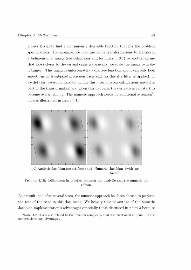
Chapter 3. Methodology 48
always trivial to find a continuously derivable function that fits the problem
specifications. For example, we may use affine transformations to transform
a bidimensional image (see definitions and formulas in 3.1) to another image
that looks closer to the virtual camera (basically, we scale the image to make
it bigger). This image is unfortunately a discrete function and it can only look
smooth in with subpixel precission cases such as this if a filter is applied. If
we did this, we would have to include this filter into our calculations since it is
part of the transformation and when this happens, the derivatives can start to
become overwhelming. The numeric approach needs no additional attention5.
This is illustrated in figure 4.10.
(a) Analytic Jacobian (no artifacts) (b) Numeric Jacobian (with arti-facts)
Figure 4.10: Differences in practice between the analytic and the numeric Ja-cobian.
As a result, and after several tests, the numeric approach has been chosen to perform
the rest of the tests in this document. We heavily take advantage of the numeric
Jacobian implementation’s advantages especially those discussed in point 3 because
5Note that this is also related to the function complexity that was mentioned in point 1 of thenumeric Jacobian advantages.

Chapter 3. Methodology 49
of our f function requirements in practice (which will be addressed in next section).
The next section will refer to how can this implementation be advantageous in RGB-
D problems.
4.2.2 RGB-D in direct methods
In this part of the document, details related to the implementation of LK and IC
in direct methods is also discussed. However, most of the theory behind the chosen
approach to deal with RGB-D based images has already been described in chapter
3, especially in section 3.1.2.
The tests presented in this document are going to be based entirely on point-clouds,
3D transformations of 6 degrees of freedom and the pinhole-camera model as stated
in section 3.1.2. We choose point-clouds because it seems to be a simple and plau-
sible standard way to produce 3D samples of any sort of volume, however, several
alternatives exist that may be more suitable in other scenarios. The transforma-
tion is the one named as T6dof3D described in section 3.1.2 which will be used in a
per-point basis. And, we choose the pinhole-camera model for the virtual camera
because it is the standard to simulate any real camera and in case these algorithms
are applied to real images, the real parameters are required.
To adopt the LK and IC algorithms as direct methods to solve our problem we need
to do slight changes to the processes that are already detailed in section 3.2. The
transformation function f becomes the function that combines the 3D transforma-
tion from 3.4 and the projection from 3.6. Using the same notation, the complete
transformation f : P3 → P2 becomes:
f : P → PS =[K 0
]· C · T6dof3D · P (4.12)

Chapter 3. Methodology 50
Since the transformations may include the grey-scale component retrieved from the
camera RGB color channels, that also has to be taken into account. But the addition
of color into our problem does not require any change in f . Each point will have
an associated color value so the only requirement in this case is to be able to track
each point during the procedure and to retrieve its color when needed.
In practice, the color values are stored alongside the point-cloud data and these
values are retrieved when the perspective projection is done. This idea is the same
that is used in [26]. They call it the extended images which in practice is the same
as the definition that has just been given in the previous paragraph. In this article,
they refer instead to two separate images with different meanings, but that is only
a definition difference since in practice the effect of the definition given here is the
same. Note that treating color alongside depth data as if it was another point means
that no preferences or biases are given towards one type of data or the other.
There is an additional problem that has not been addressed in the previous defini-
tion of f . Projecting points into the virtual camera plane is needed because we are
assuming that we are given two images, thus two planes with color values associ-
ated to their coordinates. But our definition 4.12 will cause unnatural incoherences
with the behavior that a real projection actually has. The lack of coherence in the
definition 4.12 stems from the fact that in reality if two points are aligned with the
camera origin, the closest point is the one that is actually projected. If the closest
point was transparent, light could pass through it leaving the farthest point partially
visible. In our problem definition, we assume that all points occlude other points
when these are aligned. Depending on the order we execute our algorithm, some
points will stand in front of other points even if these points are not closer. This
means that previous definition also requires a check of priorly projected points in
the screen or, alternatively, it needs to reorder aligned points (actually, there are
more possible alternatives to solve this).

Chapter 3. Methodology 51
In practice, we project all these points into discrete images and one point may fill
up to one pixel once projected. So the only thing left to do is to check if a given
pixel of the final image already has a depth value that is lower than the newer value.
This task can be considered inside the definition of f or even in the definition of I
and T as functions. The image function I can be seen as the function that iterates
over all the transformed points PS in screen coordinates and that returns the closest
point to the camera in the pixel that we are asking for. The resulting algorithm
for a single point P assuming that color values are also provided would be the one
shown in figure 4.2.
Algorithm 4.1: Projection algorithm in RGB-D
Input: point P from point-cloud and its associated color g in grey-scaleTransform P into PS using f from definition 4.12Create temporary space for the warped image IwTransform PS coordinates into discrete pixel coordinates performing a perspectivedivide PS/λ (acquire indices (i, j) after this division to access matrix Iw)if λ closer than Iw(i, j) then
Store λ in IwStore g in IwNote: this conditional branch is the only thing that cannot be executed inparallel though it can be executed with certain parallelism for those points thatdo not lie in the same target pixel.
end
Apart from this procedure, it is also common to fill neighboring pixels as if the
current point was actually larger. This is usually done while rendering point-clouds
in geographical applications. It is a very important thing to do because after a
transformation, some points may be too close to the camera and gaps between
them will become visible. In general, we want to have something that resembles a
continuous surface as much as possible as illustrated in figure 4.11.
This last issue together with the algorithm stated before are examples of f functions
and compositions of functions that are done during the warping phase and that

Chapter 3. Methodology 52
(a) No gaps when the pointcloud isdenser.
(b) Gaps when the camera is closeto a finer pointcloud.
Figure 4.11: Different pointcloud resolutions.
tend to be very difficult to differentiate analytically. This supports our idea of using
numeric Jacobians for this task.
Our new version of LK and IC assume that points P are given instead of images
but we also have to assume that an input image and a template image in grey-scale
format, depth format or both are gathered by a camera or any other device at the
beginning. These are bidimensional images that have to represent the depth or
color of several sampled points so it is also required to make a prior transformation
of these images into point-clouds. In order to do this a reverse.
LK and IC can be easily adapted to the new transformation and model definitions.
The algorithms 3.1 and 3.2 only require the addition of an off-line step that must be
done before the any other step in those algorithms. This step is the deprojection step
which generates the associated point-cloud and their colors. In LK the deprojection
must be performed over I since this is the image that is going to be warped in
each iteration and it is also the image that is going to be differentiated. In IC, the
deprojection is required over I and also T , I is warped at every step as well and T

Chapter 3. Methodology 53
is the image that is used for the Jacobian so the point-cloud is also needed. The
deprojection algorithm can be executed in parallel for each pixel.
Algorithm 4.2: Deprojection algorithm in RGB-D.
Input: depth image Id and color image Ig in grey-scalePerspective multiply in each pixel [i, j] · λ and generate PSTransform PS into P using the inverse definition of f , formally described at 4.13Store coordinates of P and store its color value
Formal definition of the inverse projection f−1 or deprojection:
f−1 : PS =
j/λ
i/λ
1/λ
→ P = T−16dof3D · C−1 ·
[K−1 0
0 1
]·
[PS
1
](4.13)
Note that in these formal definitions PS carries the depth values λ so that the actual
values are calculated after doing the perspective multiply.
The deprojection could also be done online in LK. In principle, it is also possible to
deproject the input image, project it again after the parameters have been updated,
then deproject this new image again and so on. The problem of this approach is
twofold. The computational cost becomes very high in comparison and even more
importantly, each time that these points are deprojected and projected again, the
errors accumulate especially for the fact that the points target a pixel and its neigh-
bors. The latter makes objects become bigger in each step since they occupy more
pixels in the image and this also accumulates. But even without this accumulation,
once a projection is done, many points are rejected because of two main reasons:
these points may be projected outside the screen so there is no point in rendering it
or this point can be completely occluded by another point.
These are the minima (plus some details like the neighbor pixels) required to im-
plement direct methods with RGB-D based images. However, there are other issues

Chapter 3. Methodology 54
that the implementer may not be aware of and they are extremely important for LK
and IC to converge.
One of these issues is the coordinate system positioning since it affects the numer-
ical conditioning of the optimization. This is a very relevant issue because of the
abundance or, in contrast, lack of ambiguity that the coordinates can cause in the
Jacobian. Independently of the Jacobian calculation method that is chosen, the
Jacobian is theoretically meant to be an infinitely small movement that we can use
to estimate qualitatively and quantitatively. In certain situations, the Jacobian of
two parameters may be so similar that methods such as LK or IC cannot decide
whether or not to follow one gradient, the other or both. This can happen in very
simple situations, for instance, if a cube is positioned very close to the center of the
coordinate system and we calculate the derivatives of a rotation over this center, the
derivatives of the closest corners of the cube are going to be much higher than those
from the farthest point. If the cube is far away from the center, both corners will
have very similar derivatives and these derivatives can be mistaken with those from
a translation (see figure 4.12, the derivatives are almost parallel when the cube is far
away from the origin). Besides, if floating-points are used to simulate real numbers,
the larger the number, the lesser the accuracy.
The second and last issue is related to occlusions. As stated in the examples of
section 4.1, LK and IC are methods that follow the gradients (local methods) to
find a local minimum or, hopefully, the global minimum. This requires that the
functions that we work with are smooth enough and continuous. If LK or IC are
applied to noisy images or images with sharp edges, it is unlikely that these methods
will ever converge unless the rest of the image is smooth enough and these sharp
points are relatively less in number than the other ones. In particular, RGB-D
images are very problematic in this sense because of occlusions. Occlusions can
cause images to have sharp edges that make the residuals have sharp edges, but not

Chapter 3. Methodology 55
(a) Derivatives when the cube isclose to the origin.
(b) Derivatives when the cube is farfrom the origin.
Figure 4.12: How different coordinate systems affect the derivatives (green forrotation derivatives and red for translation derivatives).
only that, occlusions can cause sharp edges in Jacobians as well and these are even
more problematic especially in images related to depth values.
To solve this, several techniques have been proposed in the literature. These tech-
niques are usually the robustness techniques and also coarse-to-fine schemes which
can help at least when convergence acceleration is desired. These have been already
presented in 3.2.4.
4.3 Synthetic models
A very brief description of the models used to perform several experiments in the
RGB-D context is presented in this section. Some of these examples have only been
created for experimentation purposes and are not used later in the thesis.

Chapter 3. Methodology 56
4.3.1 Finite plane
The finite plane may be the easiest way to test how well LK and IC perform. It
can also serve to understand which ambiguities affect direct methods in RGB-D
contexts.
The finite plane is a very ambiguous model when used with depth values and at
the same time when it occupies the whole screen space. The depth values of an
infinite plane remain the same after several sorts of warps. Definitely, warps like
any rotation of the plane over its normal vector or any translation of the plane over
itself or the combination of both yields another plane with the same exact depth
values. Other warps do not share this problem.
When color is added to the plane, warps start being less ambiguous as long as the
images used for the colors are not relatively ambiguous by themselves. For example,
if an image of a circle is chosen, rotations over the center of this circle are still
ambiguous even if the circle is the texture of a plane. In general, any ambiguity in
a 2D scenario will still be ambiguous in a 3D plane in the same warps noted before
with the depth values. Cases like this one support the idea of using depth and color
data together so that ambiguities from some data are relaxed by other data.
This model has been created for the cube that is going to be employed to analyze
LK and IC behavior. In case the reader is interested, the article [35] offers results
of several tests using a finite plane model with 4 Gaussians distributions as their
texture but with no depth values.
4.3.2 Simple cube
This model simulates three faces of a cube. Those faces that are visible from the
camera perspective. In case that the tests require color data, the texture applied to

Chapter 3. Methodology 57
each face is the 4 Gaussian distributions image already shown in figure 4.8. Note
that these three faces are rendered exactly in the same way as the finite plane but
using three finite planes instead of one.
This cube is positioned in space in the following way. The cube’s edges are aligned
with the positive XYZ axis and the visible corner in the images is actually the
coordinate origin [0, 0, 0]. The cube’s three main and visible faces occupy all the
values (depending on the sample resolution) from 0 to 1 in the XYZ positive axis.
This model has been chosen for extensive testing because a cube can be rendered
having one of its faces almost perpendicularly to the camera while the other faces are
in very extreme and unfavorable conditions for algorithms based on direct methods.
The camera has been zoomed and centered in one of the corners of the cube and
oriented in parallel with the diagonal axis of the cube. This helps to avoid sharp
edges due to silhouettes and occlusions against the background in depth images
(see figures 4.13 and 4.14, note that in depth images, darker colors are closer to the
camera than brighter colors). Grey scale images do not have the same problems since
by default the background is set to black and the textures that are used are very dark
near the edges. Furthermore, the Jacobians are calculated using the whole image
while the actual image used for the residuals is a reduced version of the original
image. This means that the original image is processed normally, but when the
increment has to be finally calculated, a smaller window selection inside the image
is used. This helps to avoid sharp edges generated after performing relatively small
warps due to the lack of information outside the image.
The input image is always rendered from the “resting” position which is depicted
in (A) and (B) in figure 4.13. Then the template image is generated from a vector
of parameters introduced by the user. This is done in this way because if there was
a case in which the cube had a face that occupied only one pixel of width, only a
straight line of points would be sampled from that face. With these samples, the

Chapter 3. Methodology 58
point cloud is generated (see 4.2.2 for more details about the deprojection algorithm)
and it would have only a straight line of samples when the underlying model is a
plane. If the cube occupies always the entire rendering target (the input image), a
very high and accurate amount of samples is taken from the cube and the test can
succeed.
The cube is the object that has been chosen to learn how far can LK and IC be
used in RGB-D and study their convergence conditions. The results are discussed
in next chapter.

Chapter 3. Methodology 59
(a) Depth image (b) Grey-scale image
(c) Depth image (d) Grey-scale image
Figure 4.13: Examples of the cube while camera not zoomed in

Chapter 3. Methodology 60
(a) Depth image (b) Grey-scale image
(c) Depth image (d) Grey-scale image
Figure 4.14: Examples of the cube while camera zoomed in

Chapter 5
Results
All the experiments have been executed using the simple cube model that has been
already introduced in the methodology section 4.3. In order to understand how
accurate each algorithm is in each situation, several combinations of parameters
have been tested and its results have been gathered. The procedure is explained in
next section.
All the tests have been executed in Ubuntu 14.04 LTS using an Intel i7-4500U CPU
at 2.00 GHz. The code is written in Python 2.7.8 using NumPy 1.8.2 for fast array
access together with Cython 0.20.1 for certain optimisations especially in projection
and deprojection. The time has been retrieved using the time package available
in Python’s standard library. Most of the graphs and images have been generated
using Matplotlib, others have been generated using Weka’s visualization tab and
other graphs have been generated using LibreOffice Calc.
61

Chapter 4. Results 62
5.1 Testing procedure
The tests have been performed using randomly sampled values for the parameters of
the generated template image in different ranges. Each input and template images
are generated as detailed in section 4.3 of the previous chapter. And since the inpu
image is common to all the tests, that image is generated only once to accelerate
the procedure.
The parameter generation procedure is similar to the one used in [35]. A total of 100
parameters are generated using random samples from a Gaussian distribution with
parameters µ = 0 and a desired σ (N (0, σ) offered in Python using random.gauss
from the random package). For a 6 dergees of freedom transformation like those
that are used in these experiments, a total of 6 parameters are required to generate
the transformation. So in each test, 6 samples are gathered from that distribution
and those samples are given to the testing tool to proceed. In order to be able to
classify tests by difficulty, the value of σ is changed every 100 tests1. The values of
σ are changed using the values from the set 0.01, 0.05, 0.1, 0.15, 0.2. Since we have 2
algorithms with 3 image variants, this means that a total of 3000 tests are generated
in the process.
All these tests have been executed using a derivative precision value of h = 0.005
and the values used as thresholds for the halting criterion in the increment are
c = 0.005 for convergence and d = 0.5 for divergence. When the increment’s norm
has reached c or d or 20 iterations have been performed, the algorithm decides to
halt. If c is reached, a convergence state is returned, when d is reached a divergence
state is returned and when the 20 iterations have been reached, we cannot decide
what could have happened. Additionally, if a Jacobian has a lower range, a singular
matrix error is detected and the state of singular matrix is returned.
1Note that increasing the value of σ just makes it more likely to get larger samples, but smallersamples are still possible, this is a desired effect so that not all the parameters are equally large.

Chapter 4. Results 63
These values have been acquired after extensive testing. Though, more testing would
be needed to obtain the best value for each parameter but that also depends on the
case. So we have chosen the values that make the results be better in general. For
instance, certain values do not even produce acceptable Jacobians or in other cases,
threshold convergence values that are too large halt the algorithms too early and if
a test would diverge, an early halt may make this test look like if it performed well.
The maximum amount of iterations to halt the algorithm is 20. When this amount
of iterations is reached, it cannot be decided if the algorithm will actually converge
to a minimum (even if this is a local minimum) or not.
The first set of tests did not yield consistent results due to the fact that h was not
small enough so the accuracy of the Jacobian was not leading the algorithms well
when the accuracy was very close. Several graphs showed that there was noise at
the end of the series of iterations.
The second set of tests had a very small h leading to singular matrices (the cluster
with around 1.5 increment norm) because there were no differences between the
transformations with such a low value.
After the process has finished performing the tests, some statistics are gathered so
that conclusions can be drawn and explained in this chapter. The statistics that are
important for us are those that measure the accuracy of our tests. The evaluation
is done calculating the Euclidean distance between 3 known points ([0, 0, 0], [1, 0, 0]
and [0, 1, 0]) and their 3 counterparts after being transformed by the initial trans-
formation done in the template and then transforming these points back to their
originals using our parameter estimation in the current test. The closer these points
are in space, the lesser the distance will be. The distances of each pair are added
to generate the measure. If the distance is too high, we say that the algorithm has
not succesfully converged to a relatively desirable solution. This desirable solution
is the convergence threshold.

Chapter 4. Results 64
The convergence threshold has been decided experimentally after observing the re-
sults obtained from several tests prior to the tests with different values of σ. To
observe the results, two tools have been used, one is Weka’s visualization tool and
the other is the result visualization available in our implementation. Weka tools can
be used to see where are the clusters of converging tests in general and these con-
vergence thresholds can be deduced from them after several test results have been
gathered. This set of tests have been used to guess the values of h, c and d as well.
The value that is going to be used to discard tests as not successfully convergent are
those surpassing a threshold of 0.2 for the 3D distance measures. Which means that
at most each point has deviated 0.2/2 = 0.1 since we are adding the distances of
the three points together and at most one point will remain static while the others
rotate.
To illustrate how much is 0.2 for a 3D error distance is, see figure 5.1 showing an
error distance of 0.22215.
(a) Target warp (b) Estimated warp
Figure 5.1: Example of a warp discarded because of its error.

Chapter 4. Results 65
5.2 Results analysis
This section provides the results and summaries obtained from the various tests
already described in the testing procedure.
5.2.1 Test sets
The cluster images that were analyzed to finally opt to certain parameters provided a
good idea of how all the algorithms perform in general terms and what the tendency
is. The first set of tests with relatively close parameters provided a very good
feedback because of the graph clarity, see figure 5.2. It can be noted that most of
the succesful results are gathered within a very tight cluster where most cases halted
with relatively low increments. The figure shows the whole dataset in two axis where
the horizontal axis is the 2D error distance and the vertical axis is the 3D distance
error that each instance ended with. Each color shows the type of algorithm and
image that was used in that test (dark-blue for LKd, red for LKg, green for LKgd,
light-blue for ICd, light pink for ICg and dark pink for ICgd where “d” refers to only
depth images, “g” refers to only grey images and “gd” means both).
The amount of failed tests for LK was unexpected especially in the depth images only.
To understand why these tests failed, a couple of examples and detailed comparisons
of the results are shown.
A first example is LK depth with parameters [0.3, 0.3, 0, 0, 0, 0]. It is compared with
the test that has parameters [0.2, 0.2, 0, 0, 0, 0] which is sufficient for our purposes.
This is shown in figures 5.3 and 5.4. In the first image, the centered window does
not have any pixel with values of the background. On the other hand, the second
image has a large portion of background pixels.

Chapter 4. Results 66
(a) Whole dataset
(b) Subset that converges
Figure 5.2: Graphs showing the relationship between 2D and 3D error distances.
In the first iteration of LK in the case of [0.3, 0.3, 0, 0, 0, 0], one realises that the
Jacobians are not suitable for good convergence because of the large discrepancy
between the residual and the Jacobians. This discrepancy has a visible effect in the

Chapter 4. Results 67
(a) Original image used as input image andits warped image as template.
(b) Residual of previous image (inside the window).
Figure 5.3: Warp of [0.2, 0.2, 0, 0, 0, 0], original images and their residuals.
proportional product (the distintion between the two products is given in section
4.1). Figure 5.5 illustrates this, the forth parameter’s derivatives is the one named
“Jp4”. The parameter “p4” is the responsible of the translations in the X axis of
the object (from left to right in the images).
When the per-pixel product (theoretically, per point) is done between the derivatives
and the residuals, the image called “prop4” is generated. This image is the first
product that was distinguished in two very simple cases in section 4.1. This image
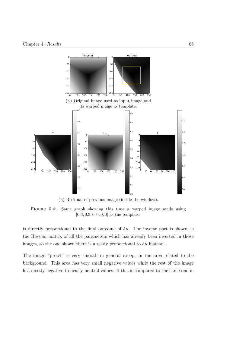
Chapter 4. Results 68
(a) Original image used as input image andits warped image as template.
(b) Residual of previous image (inside the window).
Figure 5.4: Same graph showing this time a warped image made using[0.3, 0.3, 0, 0, 0, 0] as the template.
is directly proportional to the final outcome of δµ. The inverse part is shown as
the Hessian matrix of all the parameters which has already been inverted in those
images, so the one shown there is already proportional to δµ instead.
The image “prop4” is very smooth in general except in the area related to the
background. This area has very small negative values while the rest of the image
has mostly negative to nearly neutral values. If this is compared to the same one in

Chapter 4. Results 69
[0.2, 0.2, 0, 0, 0, 0], the difference is tangible. Obviously, both examples have exactly
the same Hessian matrix in LK and the vectors of the proportional part of each
parameter are also very similar apparently in those images. If one looks closer, the
values in provided in the right side color bars for each plot, the values are much
more distant than those from the easier example shown in figure A. These values
are relatively more negative and their absolute value is much larger than the others.
Since the Hessian is the same, it is clear at this point that the increment δµ of the
example with background is going to be much more exaggerated due to the simple
fact that the background was present.
These effects of the background in the IC are less noticeable. Figure 5.6 shows the
information as the figures that were referenced before but in IC with parameters
[0.3, 0.3, 0, 0, 0, 0]. It is still the first iteration in the algorithm. It can be noted that
the values are very extreme starting with the Jacobian. There is no relative smooth-
ness and there only exists a single sharp edge, the one between the cube and the
background. The Jacobian in IC is very different this time because the information
is provided by the target instead of the starting point. All the values are extreme
in all the Jacobian images for every parameter, that is the reason behind such small
values in the Hessian matrix. The difference in orders of magnitude between the
Hessian values and the porportional vector values is much more pronounced than
the difference in LK, even in the difference in LK for the easier example. This entails
that the convergence or divergence of this example is very slow. Since a maximum of
20 iterations is set, the algorithm does not diverge as fast as LK does. It is our belief
that this is the main explanation behind those divergent cases in LK shown in figure
5.2. Besides, this does not happen in grey-scale images because the background is
black and the textures are mostly black in the edges.
The results of these examples in [0.3, 0.3, 0, 0, 0, 0] with LK and IC are presented in
figure 5.7.

Chapter 4. Results 70
(a) Jacobian in LK with warp [0.2, 0.2, 0, 0, 0, 0].
(b) Jacobian in LK with warp [0.3, 0.3, 0, 0, 0, 0].
Figure 5.5: Comparison of Jacobians in both examples.

Chapter 4. Results 71
Figure 5.6: Again the same graph but in IC.
5.2.2 Overall results
These are the overall results obtained from the 3000 tests set that has been explained
in detail before. The overall results are shown following the same ideas of three plots
proposed in [35]. Each plot describes:
• Robustness plot: this plot shows the percentage of successes that have been
found in our tests for each algorithm and type of image and σ (figure 5.8).
• Accuracy plot: for those tests that have successfully converged, the accuracy
is compared also with varying σ (figure 5.9).
• Rate of convergence plot: in this plot, also the successful tests are taken
into account. The plot shows regardless of the value of σ the accuracy (error
distance) of each algorithm in each kind of image (figure 5.10).

Chapter 4. Results 72
(a) Input, resulting and template images in LK example.
(b) Input, resulting and template images in IC example.
Figure 5.7: Comparison of images in the example with parameters[0.3, 0.3, 0, 0, 0, 0].
The robustness plot shows clearly that all the algorithms that use depth values tend
to work better than those based on grey-scale images. This confirms that depth
values are indeed good sources of information to estimate transformations of rigid
bodies. The reader should note that the warps at higher values of σ tend to be
very complicated to estimate so it is just logical that the results of all algorithms
tend to decrease in a very constant pace. As expected Lucas-Kanade offers the best
results in every combination against those from IC. Though IC is very close to LK
when used together with depth images. So this also confirms that IC can be used
for image alignment tasks using depth images.
Unfortunately, it seems that IC cannot work well in any case when mixing both
sorts of images. This was actually an unexpected result so a question remains open,
we still do not know how to combine well both data so that it works better in IC.

Chapter 4. Results 73
Figure 5.8: Robustness plot
Figure 5.9: Accuracy plot
IC performs very well with depth images so the expected behavior would be that
depth images would compensate for the bad results obtained in IC with grey-scale

Chapter 4. Results 74
Figure 5.10: Rate of convergence plot
values. The reason behind this is likely to be the fact that IC cannot work well with
grey scale images as stated in [35] because it does not satisfy the EBCA condition.
It seems that the grey values can be very confusing and any sort of alteration can
lead to very unstable results such as this one.
LK appears to perform poorly especially in comparison to the results obtained with
depth images. In this case, LK does actually benefit from depth data since it per-
forms as well as those with just depth data. So it is very clear at this point that
grey-scale values are not a very good option to estimate 3D transformations as a
whole. Not even images that are as smooth as the ones used in these tests. This
may seem to contradict our thoughts about LK. LK was supposed to perform well
in every scenario, even though it was expected that the worst scenario would be the
grey scale images. But there is a plausible explanation behind this. If the accuracy
plot is checked, IC with grey values seems to be getting a worse accuracy with every
sigma increase while curiously, the opposite happens with LK. The last sigma (0.2)
does not count as much in this plot for LKg, ICg or LKgd because this average was

Chapter 4. Results 75
calculated from just 4 to 6 tests that passed the convergence criterion2. Note that
in the robustness plot and in the rate of convergence plot ICgd does not even exist
in these plots because there are no tests that have succesfully converged.
Finally, the last plot, the rate convergence, shows a very clear result that summarizes
and cofirms all the assumptions. It seemed confusing that ICg could have so good
results and especially so close to LKg. However, this is just apparent. When figure
5.10 is analyzed, it is clear that all the tests that have been classified as succesful
start on average with a more difficult situation (the error at the beginning is higher)
than LKg but especially than ICg. ICg tests that succesfully converge start with
a distance that is even smaller than the criterion on average so the algorithm just
needs to converge close to the starting point and the results will of course be very
satisfactory. But even with such an advantage, these tests that converge actually
tend to diverge over time since the graph shows that the error tends to increase
while in the other algorithms decrease. This graph also shows that LKg converges
but maybe 20 iterations before halting is not enough for LKg to converge well.
So in any case, this graph shows that using grey-scale images for these tasks is
counterproductive in general.
2Check the robustness plot to see that all these tests are close to a 0 percent and therefore, ifa couple of tests have relatively large values or relatively small, the average is seriously affected


Chapter 6
Conclusions
In general the experiments have confirmed our first impression that depth images
serve as a good guidance for direct methods towards a global optimum, mainly be-
cause of their smoothness. The difference between the accuracy obtained from depth
values and the accuracy obtained from grey scale values is even more significative
because of the lack of difficulty in the synthetic tests that have been proposed and
used. This was expected and now is confirmed.
There is one detail that was not entirely expected. The experiments have also shown
that combining both images equally (using the extended image definition from [26])
does not work as well as we thought it would at the beginning of the research
process. It was expected that when combining both images, the depth data would
have a better effect over the algorithm’s outcome in comparison to grey scale data
on its own. But the results show that in IC this is not the case and the results are
the worst by far.
The results have also confirmed our most relevant hypothesis, that IC performs
very well in depth images but that it is not suitable for grey scale images. This
was already known from the studies done in [35] according to the theory behind
77

Chapter 5. Conclusions 78
the EBCA. LK outperforms IC in all the tests where grey scale data is involved.
As it has already been stated, IC is seriously affected by grey scale values and
the increment step seems to get contaminated to the point that it tends to slowly
diverge. In our data, the convergence of IC with grey scale images is reasonable
but that is because of the fact that there is a maximum amount of iterations and
the process has not been tested long enough to actually make the algorithm to lie
outside the convergence threshold that we have established. However, according
to our results, the convergence of IC in these images decreases substantially as the
iterations advance but the other methods do not share this problem.
These results will let future students or researchers study and address the particular
problems that have been detected for each algorithm and each case to mitigate these
problems using other techniques in conjunction with these algorithms.
6.1 Future work
Several lines of future work are opened for further research. Each one of the ideas
that were out of the scope of this thesis are detailed in the following list:
• It is necessary to perform more tests but using different models and especially
different textures for the grey-scale images. These models should be more chal-
lenging than a cube so that further studies can be made in order to understand
better the behavior of these algorithms.
• Since the high contrast between the depth of the background and the depth
of the object lead to mistakes, it is necessary to at least create an algorithm
that solves this issue and afterwards, these tests could be reused to see if
the algorithm is capable of improving the results in comparison to the results
obtained here.

Chapter 5. Conclusions 79
• These tests could be accelerated so that the implementation could be used
even in real-time with data retrieved from a depth camera.


Appendix A
Kinect and OpenCV
Figure A.1: The Kinect device.
The installation of the Kinect device for Ubuntu OS is detailed in this appendix.
The installation procedure has been tested in April 2015 in a system with Ubuntu
14.04 LTS installed. This procedure should be also very similar for other Linux
distributions.
81

Appendix A. Kinect setup 82
In order to install and use the Kinect device, at least one USB connection is required.
The software needed prior to the main installation process can be installed using the
following command (these are not multiple commands but a large single command).
sudo apt-get install git-core cmake freeglut3-dev \\
pkg-config build-essential libxmu-dev libxi-dev \\
libusb-1.0-0-dev doxygen graphviz mono-complete
The following procedure is the one needed to install the device via OpenNI and
OpenCV:
Installation of OpenNI 1.5.x, type the following commands in a terminal from your
home directory or any other place where the OpenNI’s source repository is going to
be downloaded:
mkdir ~/kinect
cd ~/kinect
git clone https://github.com/OpenNI/OpenNI.git
cd OpenNI/Platform/Linux/CreateRedist/
chmod +x RedistMaker
./RedistMaker
cd ../Redist/OpenNI-Bin-Dev-Linux-x64-v1.5.7.10/
sudo ./install.sh
Download PrimeSense drivers for Kinect from a repository as well:
cd ~/kinect/
git clone git://github.com/avin2/SensorKinect.git

Appendix A. Kinect setup 83
Before installing, change 2 files using the code available at https://github.com/
avin2/SensorKinect/pull/5/files#diff-181b87ab5e036090aa9a6cb65e715212 (checked
site availability in July 2015). Then substitute the files under source/XnDeviceSen-
sorV2 with those available at the given URL.
Proceed with the installation of the drivers:
cd SensorKinect/Platform/Linux/CreateRedist/
chmod +x RedistMaker
./RedistMaker
cd ../Redist/Sensor-Bin-Linux-x64-v5.1.0.25/
chmod +x install.sh
sudo ./install.sh
Installation of OpenCV using the latest stable version available at http://sourceforge.
net/projects/opencvlibrary/ (checked site availability in July 2015). Then un-
compress it and do the following in the directory:
cd ~/opencv-2.4.11/
mkdir release
cd ./release/
cmake -D WITH_OPENNI=ON ..
Check that OpenNI and PrimeSense modules have the flag ”yes” in the ending
summary, then:
make
sudo make install
Finally, install the non-free OpenCV modules:

Appendix A. Kinect setup 84
sudo add-apt-repository --yes ppa:xqms/opencv-nonfree
sudo apt-get update
sudo apt-get install libopencv-nonfree-dev
After this, the Kinect sensor should be available as an accessible class via C++
named VideoCapture in OpenCV. Some code samples to access to the data are
provided at http://docs.opencv.org/doc/user_guide/ug_highgui.html. This
class allows the user not only to collect image data from the sensor but also to access
some of the device’s internal information such as calibration data or to enable lense
distortion correction.
Alternatively, it is also possible to calibrate the Kinect sensor to get your own version
of the intrinsic parameters of the cameras. In order to do so, there is practical guide
that explains in detail the steps that have to be followed, see reference [40].
There are other ways to access, for example, OpenKinect is another library that
can access the Kinect data streams but not the calibration data nor other internal
information of the device. The installation process is much simpler and it can also be
found at [40]. OpenKinect provides wrappers to several languages and it is very easy
to use. There are interesting examples available at https://github.com/amiller/
libfreenect-goodies (checked site availability in July 2015).
Another alternative is to use the ROS (Robotics Operating System) packages at
http://wiki.ros.org/Packages (checked site availability in July 2015). The Kinect
interface to access within ROS and the drivers are available at http://wiki.ros.
org/freenect_stack. They also have detailed instructions about how to calibrate
RGB cameras and, in particular, the depth sensor http://wiki.ros.org/kinect_
node/Calibration (checked site availability in July 2015).

Bibliography
[1] Enrique Munoz Corral. Efficient Model-based 3D Tracking by Using Direct
Image Registration. PhD thesis, Facultad de Informatica, 2012.
[2] Richard Szeliski and Heung-Yeung Shum. Creating full view panoramic im-
age mosaics and environment maps. In Proceedings of the 24th annual con-
ference on Computer graphics and interactive techniques, pages 251–258. ACM
Press/Addison-Wesley Publishing Co., 1997.
[3] Richard Szeliski. Image alignment and stitching: A tutorial. Foundations and
Trends R© in Computer Graphics and Vision, 2(1):1–104, 2006.
[4] Carol Martinez, Luis Mejias, and Pascual Campoy. A multi-resolution image
alignment technique based on direct methods for pose estimation of aerial vehi-
cles. In Digital Image Computing Techniques and Applications (DICTA), 2011
International Conference on, pages 542–548. IEEE, 2011.
[5] George Papandreou and Petros Maragos. Adaptive and constrained algorithms
for inverse compositional active appearance model fitting. In Computer Vision
and Pattern Recognition, 2008. CVPR 2008. IEEE Conference on, pages 1–8.
IEEE, 2008.
[6] Lisa Gottesfeld Brown. A survey of image registration techniques. ACM com-
puting surveys (CSUR), 24(4):325–376, 1992.
85

Bibliography 86
[7] Barbara Zitova and Jan Flusser. Image registration methods: a survey. Image
and vision computing, 21(11):977–1000, 2003.
[8] JB Antoine Maintz and Max A Viergever. A survey of medical image registra-
tion. Medical image analysis, 2(1):1–36, 1998.
[9] Bruce D Lucas, Takeo Kanade, et al. An iterative image registration technique
with an application to stereo vision. In IJCAI, volume 81, pages 674–679, 1981.
[10] Gregory D Hager and Peter N Belhumeur. Efficient region tracking with para-
metric models of geometry and illumination. Pattern Analysis and Machine
Intelligence, IEEE Transactions on, 20(10):1025–1039, 1998.
[11] Heung-Yeung Shum and Richard Szeliski. Systems and experiment paper: Con-
struction of panoramic image mosaics with global and local alignment. Inter-
national Journal of Computer Vision, 36(2):101–130, 2000.
[12] Simon Baker and Iain Matthews. Equivalence and efficiency of image alignment
algorithms. In Computer Vision and Pattern Recognition, 2001. CVPR 2001.
Proceedings of the 2001 IEEE Computer Society Conference on, volume 1, pages
I–1090. IEEE, 2001.
[13] He Zhao. Inverse compositional method.
[14] Simon Baker and Iain Matthews. Lucas-kanade 20 years on: A unifying frame-
work. International journal of computer vision, 56(3):221–255, 2004.
[15] Freedeeric Jurie and Michel Dhome. Hyperplane approximation for template
matching. Pattern Analysis and Machine Intelligence, IEEE Transactions on,
24(7):996–1000, 2002.
[16] Alper Yilmaz, Omar Javed, and Mubarak Shah. Object tracking: A survey.
Acm computing surveys (CSUR), 38(4):13, 2006.

Bibliography 87
[17] Yi Wu, Jongwoo Lim, and Ming-Hsuan Yang. Online object tracking: A bench-
mark. In Computer vision and pattern recognition (CVPR), 2013 IEEE Con-
ference on, pages 2411–2418. IEEE, 2013.
[18] Zheng Fang and Yu Zhang. Experimental evaluation of rgb-d visual odometry
methods. International Journal of Advanced Robotic Systems, 12, 2015.
[19] Richard A Newcombe, Shahram Izadi, Otmar Hilliges, David Molyneaux, David
Kim, Andrew J Davison, Pushmeet Kohi, Jamie Shotton, Steve Hodges, and
Andrew Fitzgibbon. Kinectfusion: Real-time dense surface mapping and track-
ing. In Mixed and augmented reality (ISMAR), 2011 10th IEEE international
symposium on, pages 127–136. IEEE, 2011.
[20] Shahram Izadi, David Kim, Otmar Hilliges, David Molyneaux, Richard New-
combe, Pushmeet Kohli, Jamie Shotton, Steve Hodges, Dustin Freeman, An-
drew Davison, et al. Kinectfusion: real-time 3d reconstruction and interaction
using a moving depth camera. In Proceedings of the 24th annual ACM sympo-
sium on User interface software and technology, pages 559–568. ACM, 2011.
[21] Carl Yuheng Ren and Ian Reid. A unified energy minimization framework
for model fitting in depth. In Computer Vision–ECCV 2012. Workshops and
Demonstrations, pages 72–82. Springer, 2012.
[22] Carl Yuheng Ren, Victor Prisacariu, Derek Murray, and Ian Reid. Star3d:
simultaneous tracking and reconstruction of 3d objects using rgb-d data. In
Computer Vision (ICCV), 2013 IEEE International Conference on, pages 1561–
1568. IEEE, 2013.
[23] Maxime Meilland, Andrew Comport, Patrick Rives, et al. A spherical robot-
centered representation for urban navigation. In Intelligent Robots and Systems
(IROS), 2010 IEEE/RSJ International Conference on, pages 5196–5201. IEEE,
2010.

Bibliography 88
[24] Maxime Meilland, Andrew Ian Comport, and Patrick Rives. Dense visual
mapping of large scale environments for real-time localisation. In Intelligent
Robots and Systems (IROS), 2011 IEEE/RSJ International Conference on,
pages 4242–4248. IEEE, 2011.
[25] Tommi Tykkala, Cedric Audras, Andrew Comport, et al. Direct iterative closest
point for real-time visual odometry. In Computer Vision Workshops (ICCV
Workshops), 2011 IEEE International Conference on, pages 2050–2056. IEEE,
2011.
[26] Cedric Audras, A Comport, Maxime Meilland, and Patrick Rives. Real-time
dense appearance-based slam for rgb-d sensors. In Australasian Conf. on
Robotics and Automation, 2011.
[27] Christian Kerl, Jurgen Sturm, and Daniel Cremers. Robust odometry esti-
mation for rgb-d cameras. In Robotics and Automation (ICRA), 2013 IEEE
International Conference on, pages 3748–3754. IEEE, 2013.
[28] Christian Kerl, Jurgen Sturm, and Daniel Cremers. Dense visual slam for
rgb-d cameras. In Intelligent Robots and Systems (IROS), 2013 IEEE/RSJ
International Conference on, pages 2100–2106. IEEE, 2013.
[29] Jurgen Sturm, Nikolas Engelhard, Felix Endres, Wolfram Burgard, and Daniel
Cremers. A benchmark for the evaluation of rgb-d slam systems. In Intel-
ligent Robots and Systems (IROS), 2012 IEEE/RSJ International Conference
on, pages 573–580. IEEE, 2012.
[30] Kevin Lai, Liefeng Bo, Xiaofeng Ren, and Dieter Fox. A large-scale hierarchical
multi-view rgb-d object dataset. In Robotics and Automation (ICRA), 2011
IEEE International Conference on, pages 1817–1824. IEEE, 2011.
[31] Youngmin Park, Vincent Lepetit, and Woontack Woo. Texture-less object
tracking with online training using an rgb-d camera. In Mixed and Augmented

Bibliography 89
Reality (ISMAR), 2011 10th IEEE International Symposium on, pages 121–126.
IEEE, 2011.
[32] Michael Krainin, Peter Henry, Xiaofeng Ren, and Dieter Fox. Manipulator and
object tracking for in-hand 3d object modeling. The International Journal of
Robotics Research, 30(11):1311–1327, 2011.
[33] Jorg Stuckler and Sven Behnke. Model learning and real-time tracking using
multi-resolution surfel maps. In AAAI, 2012.
[34] Richard Hartley and Andrew Zisserman. Multiple view geometry in computer
vision. Cambridge university press, 2003.
[35] Enrique Munoz, Pablo Marquez-Neila, and Luis Baumela. Rationalizing effi-
cient compositional image alignment. International Journal of Computer Vi-
sion, 112(3):354–372, 2015.
[36] Jean-Yves Bouguet. Pyramidal implementation of the affine lucas kanade fea-
ture tracker description of the algorithm. Intel Corporation, 5:1–10, 2001.
[37] Frank Steinbrucker, Jurgen Sturm, and Daniel Cremers. Real-time visual odom-
etry from dense rgb-d images. In Computer Vision Workshops (ICCV Work-
shops), 2011 IEEE International Conference on, pages 719–722. IEEE, 2011.
[38] Sebastian Klose, Peter Heise, and Aaron Knoll. Efficient compositional ap-
proaches for real-time robust direct visual odometry from rgb-d data. In Intel-
ligent Robots and Systems (IROS), 2013 IEEE/RSJ International Conference
on, pages 1100–1106. IEEE, 2013.
[39] David Jimenez-Cabello. Correction of Errors in Time of Flight Cameras. PhD
thesis, Universidad de Alcala, Escuela Politecnica Superior, Departamento de
Electronica, 2015.

Bibliography 90
[40] Marina von Steinkirch. Introduction to the microsoft kinect for computational
photography and vision. 2013.
![CV3: Visual Exploration, Assessment, and Comparison of CVsVisualCV [Vis], EnhanCV [Enh], Vizualize.me [Viz], and DoY-ouBuzz [DoY]. People working as hiring managers must carry the](https://img.pdfslide.us/doc/110x75/5ed72900c30795314c174ece/cv3-visual-exploration-assessment-and-comparison-of-cvs-visualcv-vis-enhancv.jpg)