UPTEC F 13 010

Examensarbete 30 hpApril 2013

Object Recognition Using Digitally Generated Images as Training Data

Anton Ericson

Teknisk- naturvetenskaplig fakultet UTH-enheten Besöksadress: Ångströmlaboratoriet Lägerhyddsvägen 1 Hus 4, Plan 0 Postadress: Box 536 751 21 Uppsala Telefon: 018 – 471 30 03 Telefax: 018 – 471 30 00 Hemsida: http://www.teknat.uu.se/student

Abstract

Object Recognition Using Digitally Generated Imagesas Training Data

Anton Ericson

Object recognition is a much studied computer vision problem, where the task is to find a given object in an image. This Master Thesis aims at doing a MATLAB implementation of an object recognition algorithm that finds three kinds of objects in images: electrical outlets, light switches and wall mounted air-conditioning controls. Visually, these three objects are quite similar and the aim is to be able to locate these objects in an image, as well as being able to distinguish them from one another. The object recognition was accomplished using Histogram of Oriented Gradients (HOG). During the training phase, the program was trained with images of the objects to be located, as well as reference images which did not contain the objects. A Support Vector Machine (SVM) was used in the classification phase. The performance was measured for two different setups, one where the training data consisted of photos and one where the training data consisted of digitally generated images created using a 3D modeling software, in addition to the photos. The results show that using digitally generated images as training images didn’t improve the accuracy in this case. The reason for this is probably that there is too little intraclass variability in the gradients in digitally generated images, they’re too synthetic in a sense, which makes them poor at reflecting reality for this specific approach. The result might have been different if a higher number of digitally generated images had been used.

ISSN: 1401-5757, UPTEC F 13 010Examinator: Tomas NybergÄmnesgranskare: Anders HastHandledare: Stefan Seipel

Sammanfattning

Datoriserad objektigenkanning i bilder ar ett omrade vars tillampningar blirfler hela tiden. Objektigenkanning anvands i alltifran teckenigenkanningi skrivna texter och kontroll av tillverkade produkter i fabriker, till denansiktsigenkanning som ofta finns i digitala kameror och pa facebook.

Detta arbete syftar till att anvanda datorgenererade bilder till att tranaupp ett objektigenkanningsprogram som skrivits i MATLAB. Objektigenkan-ningen anvander sig av metoden Histogram of Oriented Gradients (HOG)for att tillsammans med en SVM-klassificerare jamfora innehallet i olika test-bilder med innehallet i traningsbilderna for att pa sa satt kunna lokaliseraobjekt i testbilderna.

De tre olika objekt programmet ska lara sig kanna igen ar vagguttag,lysknappar samt en vaggmonterad klimatanlaggnings-kontroll. Dessa ob-jekt ar relativt lika till utseendet, och utgor darfor utmanande men lampligamal for ett objektigenkanningsprogram. De datorgenererade bilderna fram-stalldes med hjalp av ett 3D-modelleringsprogram. Cirka 150 datorgener-erade bilder per klass anvandes sedan tillsammans med cirka 200 fotografierper klass till att trana upp programmet.

Resultatet visar att programmets precision inte forbattrades av att utokauppsattningen av traningsbilder genom att lagga till de datorgenereradebilderna. En trolig forklaring till detta ar att de datorgenererade bilderna arfor syntetiska, det ar for lite variation i gradienterna for att de ska aterspeglaverkligheten. Eventuellt kan resultatet forbattras om fler datorgenereradebilder anvands.

3

Contents

1 Introduction 5

2 Theoretical background 62.1 Structural and decision-theoretic approaches . . . . . . . . . . 62.2 The SIFT descriptor . . . . . . . . . . . . . . . . . . . . . . . 62.3 The shape context descriptor . . . . . . . . . . . . . . . . . . 72.4 The histogram of oriented gradients descriptor . . . . . . . . 82.5 Classifiers . . . . . . . . . . . . . . . . . . . . . . . . . . . . . 12

2.5.1 AdaBoost . . . . . . . . . . . . . . . . . . . . . . . . . 122.5.2 Support vector machines (SVM) . . . . . . . . . . . . 12

2.6 Related work . . . . . . . . . . . . . . . . . . . . . . . . . . . 13

3 Methods 153.1 Sliding window method . . . . . . . . . . . . . . . . . . . . . 153.2 SVM classification voting strategy . . . . . . . . . . . . . . . 153.3 Creating the 3D models . . . . . . . . . . . . . . . . . . . . . 15

4 Implementation and testing 184.1 Implementation of the object recognition . . . . . . . . . . . . 184.2 Training images and test images . . . . . . . . . . . . . . . . 20

4.2.1 Varying the image sizes . . . . . . . . . . . . . . . . . 234.2.2 False positives . . . . . . . . . . . . . . . . . . . . . . 23

4.3 Image scanning algorithm . . . . . . . . . . . . . . . . . . . . 24

5 Results 265.1 Varying size of training images . . . . . . . . . . . . . . . . . 265.2 Performance when including digitally generated images . . . . 28

6 Discussion and conclusions 306.1 Discussions on performance . . . . . . . . . . . . . . . . . . . 306.2 Concluding remarks . . . . . . . . . . . . . . . . . . . . . . . 31

4

1 Introduction

Object recognition is a task in computer vision where the aim is to findspecific objects in images using a computer. Humans are very good at doingthis effortlessly, even for objects that are occluded, and the rotation, scaleand size of the object is seldom an issue. For a computer however, this is stilla challenge and even the most advanced systems come nowhere near humanperformance. As noted by Liter and Bulthoff [16] computers do surpasshumans in certain areas of object recognition, e.g. manufacturing controlwhere they can detect small manufacturing flaws that would go unnoticedby most humans. At the same time it is difficult to give a computer thevisual capacity of a three year old, e.g. distinguishing her own toys from herfriend’s.

Object recognition applications are found in many circumstances, such asface and human recognition in images [19], character recognition of writtentext [2], assisted driving systems [10] and manufacturing quality control [4].Most object recognition approaches require a training data set, which consistof images containing the object to be recognized. Training data sets needto contain quite a large number of images to be effective, and for the mostcommon objects (e.g. humans, faces and cars) there are good databasesof training images freely downloadable from the internet. For less commonobjects however, it is often required that the training images are gatheredmanually. Constructing a set of training images based on photos is timeconsuming, and if digitally generated images could be used instead a greatdeal of work could be saved.

The three objects that are to be recognized are electrical outlets, lightswitches, and a wall mounted air-conditioning control system called LindabClimate (from now on referred to as Lindab). These objects are quite similarto each other, which make them challenging but suitable targets for objectrecognition.

The question that is to be answered in this paper is the following: canimages generated from 3D models be used as training images for computervision purposes?

To get a feeling for how the size of the images influence the recognitionresults, an evaluation of performance for different sizes of the training imageswill be carried out. This will be done without any digitally generated imagesincluded in the training image set.

5

2 Theoretical background

For humans, object recognition is nothing more than visual perception offamiliar items. But as put by Gonzalez and Woods [11], for computers,object recognition is perception of familiar patterns. The two principalapproaches for pattern recognition for computer vision purposes are decision-theoretic and structural approaches. Decision-theoretic approaches are basedon quantitative descriptors (for instance size and texture) and structuralapproaches are based on qualitative descriptors, e.g. using symbolic featuressuch as knowledge of the interspatial relations between different parts ofan object. In other words, for decision-theoretic approaches a classifier istrained with a finite number of classes and when subjected to a new patternit categorizes it into the class of best fit. Structural approaches representthe patterns as something else (e.g. graphs or trees) and the descriptors andcategorizations are based on the representations.

2.1 Structural and decision-theoretic approaches

Structural approaches come in various designs, but they all use an alternativerepresentation of some sort which their categorizations are based on. Part-based models, as mentioned in [8], form one class of structural approaches inwhich various parts of an object are located separately and the categoriza-tion is carried out using knowledge of the relative positions of these parts.This type of approach can be especially useful since different classes containsimilar parts, e.g. cars, busses and trucks all have wheels and doors. Thesetype of approaches make it possible to categorize an object without havingseen that kind of object before, by merely recognizing it’s parts.

Three common decision-theoretic approaches are the SIFT descriptor[17], the HOG descriptor [6] (the HOG descriptor is the one used in thisproject), and the Shape Context descriptor, and especially the first twoare described thoroughly in [8]. These approaches are invariant to imagetranslation, rotation and scale, which are very important qualities for objectrecognition techniques.

2.2 The SIFT descriptor

The SIFT descriptor [17] is a method that extracts “interesting points” froman image, points that are invariant to translation, rotation and scale, as wellas small changes in illumination, object pose and image noise. The points areusually located on the edges in an image. The first step in the SIFT method

6

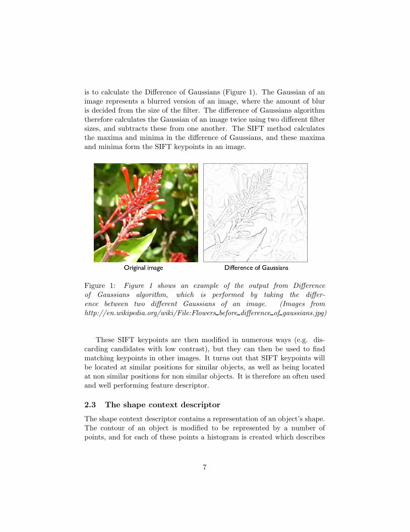
is to calculate the Difference of Gaussians (Figure 1). The Gaussian of animage represents a blurred version of an image, where the amount of bluris decided from the size of the filter. The difference of Gaussians algorithmtherefore calculates the Gaussian of an image twice using two different filtersizes, and subtracts these from one another. The SIFT method calculatesthe maxima and minima in the difference of Gaussians, and these maximaand minima form the SIFT keypoints in an image.

Figure 1: Figure 1 shows an example of the output from Differenceof Gaussians algorithm, which is performed by taking the differ-ence between two different Gaussians of an image. (Images fromhttp://en.wikipedia.org/wiki/File:Flowers before difference of gaussians.jpg)

These SIFT keypoints are then modified in numerous ways (e.g. dis-carding candidates with low contrast), but they can then be used to findmatching keypoints in other images. It turns out that SIFT keypoints willbe located at similar positions for similar objects, as well as being locatedat non similar positions for non similar objects. It is therefore an often usedand well performing feature descriptor.

2.3 The shape context descriptor

The shape context descriptor contains a representation of an object’s shape.The contour of an object is modified to be represented by a number ofpoints, and for each of these points a histogram is created which describes

7

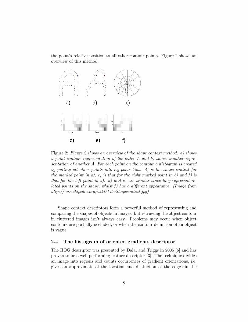
the point’s relative position to all other contour points. Figure 2 shows anoverview of this method.

Figure 2: Figure 2 shows an overview of the shape context method. a) showsa point contour representation of the letter A and b) shows another repre-sentation of another A. For each point on the contour a histogram is createdby putting all other points into log-polar bins. d) is the shape context forthe marked point in a), e) is that for the right marked point in b) and f) isthat for the left point in b). d) and e) are similar since they represent re-lated points on the shape, whilst f) has a different appearance. (Image fromhttp://en.wikipedia.org/wiki/File:Shapecontext.jpg)

Shape context descriptors form a powerful method of representing andcomparing the shapes of objects in images, but retrieving the object contourin cluttered images isn’t always easy. Problems may occur when objectcontours are partially occluded, or when the contour definition of an objectis vague.

2.4 The histogram of oriented gradients descriptor

The HOG descriptor was presented by Dalal and Triggs in 2005 [6] and hasproven to be a well performing feature descriptor [3]. The technique dividesan image into regions and counts occurrences of gradient orientations, i.e.gives an approximate of the location and distinction of the edges in the

8

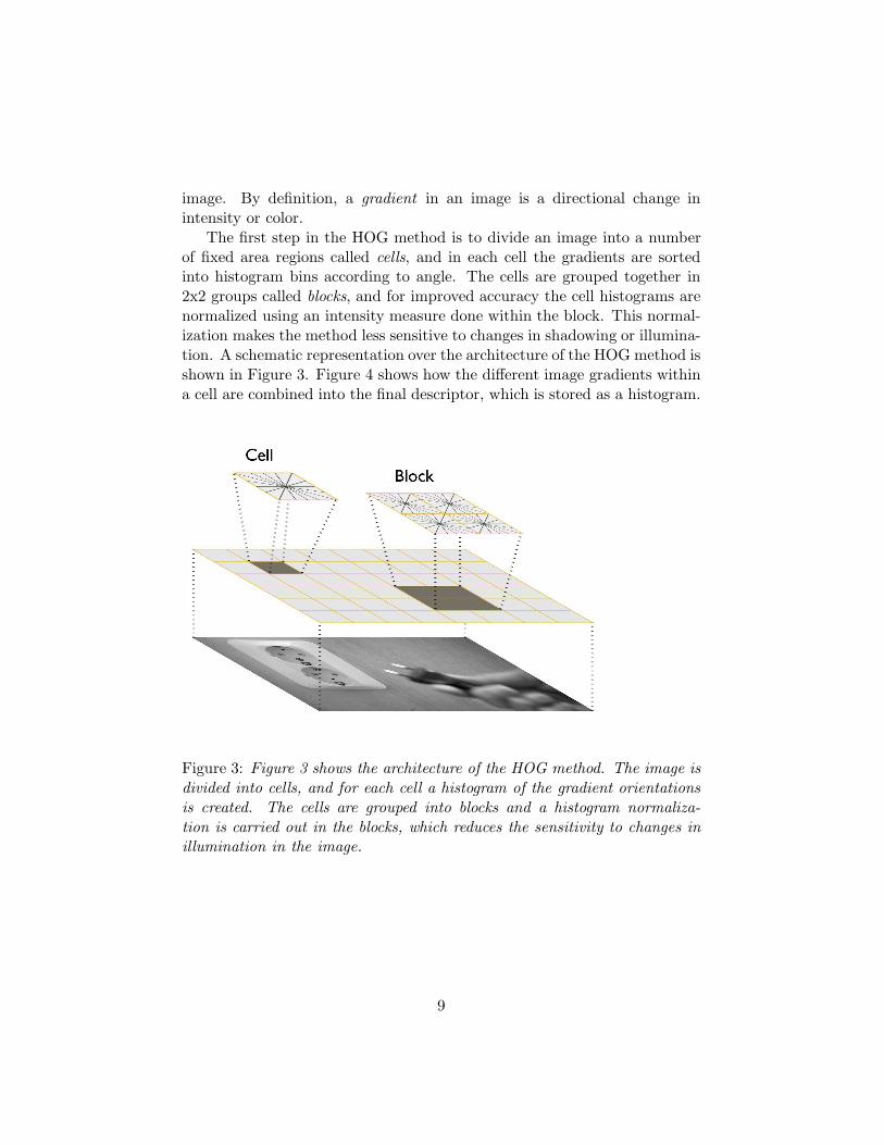
image. By definition, a gradient in an image is a directional change inintensity or color.

The first step in the HOG method is to divide an image into a numberof fixed area regions called cells, and in each cell the gradients are sortedinto histogram bins according to angle. The cells are grouped together in2x2 groups called blocks, and for improved accuracy the cell histograms arenormalized using an intensity measure done within the block. This normal-ization makes the method less sensitive to changes in shadowing or illumina-tion. A schematic representation over the architecture of the HOG method isshown in Figure 3. Figure 4 shows how the different image gradients withina cell are combined into the final descriptor, which is stored as a histogram.

Figure 3: Figure 3 shows the architecture of the HOG method. The image isdivided into cells, and for each cell a histogram of the gradient orientationsis created. The cells are grouped into blocks and a histogram normaliza-tion is carried out in the blocks, which reduces the sensitivity to changes inillumination in the image.

9

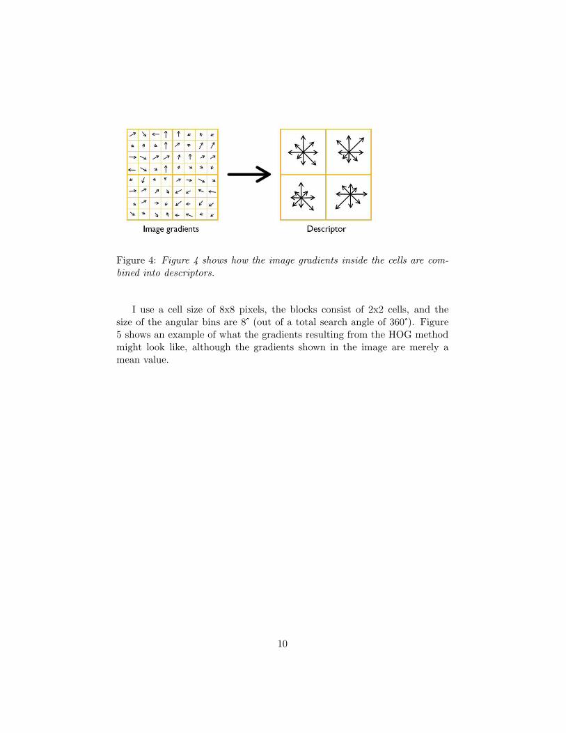
Figure 4: Figure 4 shows how the image gradients inside the cells are com-bined into descriptors.

I use a cell size of 8x8 pixels, the blocks consist of 2x2 cells, and thesize of the angular bins are 8 (out of a total search angle of 360 ). Figure5 shows an example of what the gradients resulting from the HOG methodmight look like, although the gradients shown in the image are merely amean value.

10

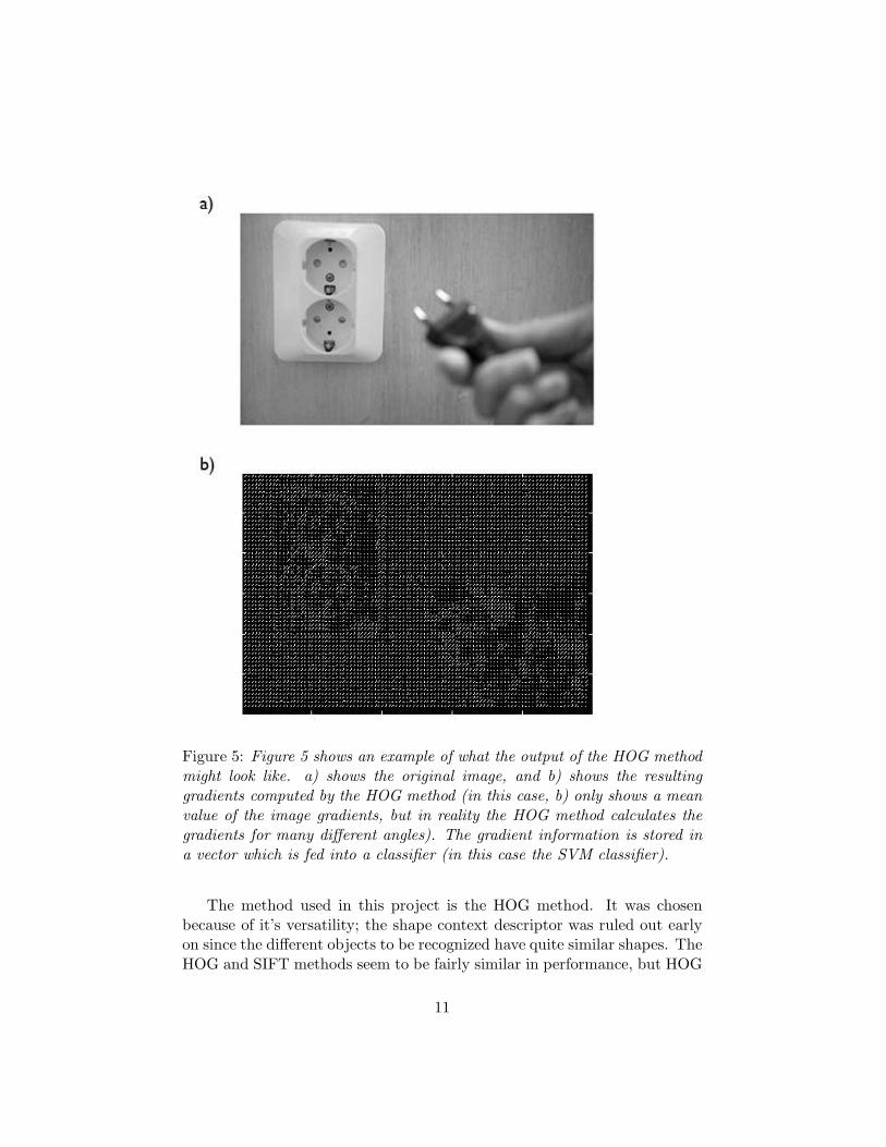
Figure 5: Figure 5 shows an example of what the output of the HOG methodmight look like. a) shows the original image, and b) shows the resultinggradients computed by the HOG method (in this case, b) only shows a meanvalue of the image gradients, but in reality the HOG method calculates thegradients for many different angles). The gradient information is stored ina vector which is fed into a classifier (in this case the SVM classifier).

The method used in this project is the HOG method. It was chosenbecause of it’s versatility; the shape context descriptor was ruled out earlyon since the different objects to be recognized have quite similar shapes. TheHOG and SIFT methods seem to be fairly similar in performance, but HOG

11

was chosen because it is conceptually simpler. Another reason for choosingHOG is that Heisele et al. use it when training their object recognitionsystem with digitally generated images [13], which is quite similar to whatwill be done in this project.

2.5 Classifiers

After the HOG descriptors have been extracted from the images, these arefed into a classifier of some sort. Many classifiers are binary, i.e. only twoclasses are handled at a time. In the training phase the classifier is fedtraining data from two different classes. When subjected to the descriptorsfrom a test image, the classifier decides which of the two classes the testimage belongs.

It is the classifier that analyzes the data and looks for the patterns thatenables a classification between different object classes. Two common ma-chine learning algorithms that are often used as classifiers in object recog-nition approaches are support vector machines (SVMs) and AdaBoost.

2.5.1 AdaBoost

AdaBoost [9] (short for Adaptive Boosting) is a machine learning algorithmthat can be used either by itself or together with other learning algorithmsto improve their performance. The general idea with AdaBoost is to takemany weak classifiers (each of which can be trained to detect a specificfeature, with a success rate of only slightly over 50%). The classifier dis-tributes weights over all the classifiers depending on their performance. TheAdaBoost classifier is highly suitable for object recognition purposes, andthere are good implementations available.

2.5.2 Support vector machines (SVM)

Support Vector Machines (SVM) [5] are linear binary classifiers which whensubjected to the descriptors from a test image look for an optimal hyperplaneas a decision function, to decide to which class the test image belongs. Thehyperplane which forms the decision function is high-dimensional, and thisis why SVMs can classify data that is not linearly separable otherwise.

For this project I decided to classify using SVMs, and the main reasonfor this was that SVMs are easier to operate than AdaBoost, as well as beingreadily available in Matlab. The SVM implementation used here is the builtin Matlab functions svmtrain and svmclassify from the BioinformaticsToolbox.

12

2.6 Related work

As mentioned earlier, in this paper I use the HOG method as feature extrac-tor, which is a decision-theoretic approach. I extend the set of images to alsoinclude digitally generated images, which in this case are images renderedusing a 3D modeling software. This is not often done for decision-theoreticapproaches, but for structural approaches it is common to use the spatialinformation from 3D models (often CAD models) to localize an object aswell as determining it’s pose.

This approach is used by Zia et al. [21] who use photorealistic renderingsof CAD models rendered from many different viewpoints as training datafor shape context descriptors [1]. Their object is to find and determine thepose of cars, and they do this by comparing the shapes in the image to thosefrom their training data.

Liebelt and Schmid [14] use an approach where a CAD model of anobject is used to learn the spatial interrelation of a class (how the differentparts are connected to each other). In this way, appearance and geometryare separated learning tasks, and provide a way to evaluate the likelihood ofdetecting groups of object parts in an image. Stark et al. [18] use a similarapproach by letting an object class be described by its semantic parts (acar for instance, is made up by the parts right front wheel, left front wheel,windshield, right front door etc). This part-based object class representationcontains constraints regarding the spatial layout as well as the relative sizesof the object parts. Another approach is the one used by Liebelt, Schmid andSchertler [15] where they extract a set of pose and class discriminant featuresfrom 3D models, called 3D Feature Maps. These synthetic descriptors canthen be matched to real ones in a 3D voting scheme.

Another common approach is to construct a 3D model of an object usinga number of 2D images, as done by Gordon and Lowe in [12]. This model canthen be fitted to the features detected in an image (Gordon and Lowe useSIFT features), and thereby acquiring the location and pose of the object.

The approach I use here is to use photorealistic renderings of 3D modelsas training images, similar to an approach used by Heisele, Kim and Meyer[13]. They use a vast number of renderings (up to 40,000 images) of 3Dmodels as training data to train a HOG classifier to detect different objects(e.g. a horse, a shoe sole etc). The test images they use are mainly digitallygenerated images as well, but they also include some photographs of theobjects. They compensate for the lack of intraclass variability in the imagesby using a vast number of images rendered from different angles, as well aschanging the light sources intensity and location relative to the object.

13

The approach chosen is similar but with a training image set consistingof both photos and digitally generated images, with a majority of the testimages being photos.

14

3 Methods

3.1 Sliding window method

The training images all depict the objects close up, filling approximately halfthe image. In order for the classification (as well as the object localization)to work properly, small sub-images of the test images must be selected andclassified one by one.

This is done using a sliding window approach, where a test image issearched a number of times with sliding windows of different sizes. In orderto reduce the risk of an area being misclassified the windows move in stepsizes equal to 1/5 of the window’s size, which means that each part of theimage is classified numerous times.

3.2 SVM classification voting strategy

The classification process is carried out in two steps: in the first step the testimage is searched using the sliding window approach, and each sub-imageis classified as containing an object or not (without determining to whichof the three objects it belongs). In step two each image area that is foundto contain an object is evaluated again, to decide to which object class thesupposed object belongs.

Since the SVM is a binary classifier and there are three different objectclasses, the classification process in step two can’t be done in only one step.To decide to which class an object candidate belongs, the one-versus-onevoting strategy is used. In this strategy, the SVM decides which of theclasses that have the highest similarity to the image; this is done by firstcomparing classes 1 and 2 to the image, then 1 and 3 and finally 2 and 3.The supposed object is sorted into the class that gets the most votes.

3.3 Creating the 3D models

Today companies often hold 3D representations of their products in the formof CAD designs, and CAD models are also widely available at e.g. Google3D Warehouse, so if images created from 3D models could facilitate in anobject recognition process much effort could be saved. Gathering all of thetraining images with a camera entails a lot of work, but creating imagesfrom 3D models is often simple in comparison.

The digitally generated images were constructed using a 3D modelingsoftware called Blender, in which digital 3D model replicas of the objectsto be recognized are built. The electrical outlet and the light switch were

15

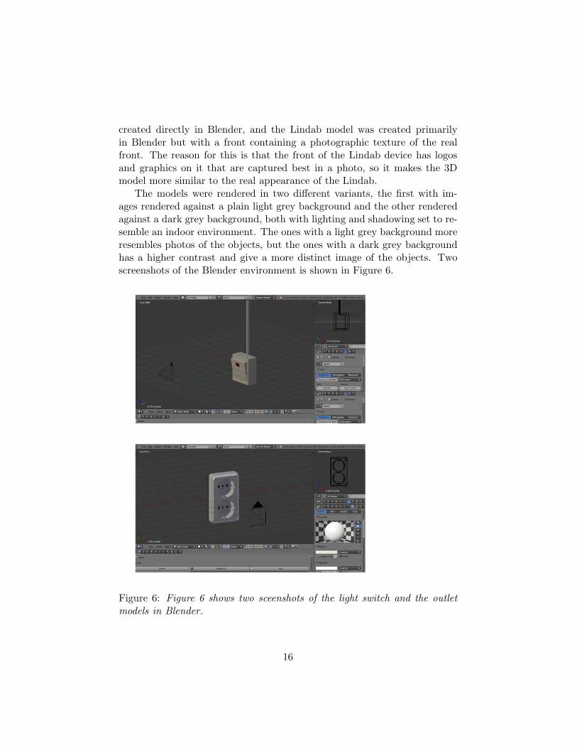
created directly in Blender, and the Lindab model was created primarilyin Blender but with a front containing a photographic texture of the realfront. The reason for this is that the front of the Lindab device has logosand graphics on it that are captured best in a photo, so it makes the 3Dmodel more similar to the real appearance of the Lindab.

The models were rendered in two different variants, the first with im-ages rendered against a plain light grey background and the other renderedagainst a dark grey background, both with lighting and shadowing set to re-semble an indoor environment. The ones with a light grey background moreresembles photos of the objects, but the ones with a dark grey backgroundhas a higher contrast and give a more distinct image of the objects. Twoscreenshots of the Blender environment is shown in Figure 6.

Figure 6: Figure 6 shows two sceenshots of the light switch and the outletmodels in Blender.

16

From these models approximately 450 images were rendered, depictingthe different objects from different angles. These images were included inthe training data set. A number of test images were also rendered, depictingthe objects included in some sort of scene, similar to the photographic testimages.

The advantage of using images rendered from 3D models is that oncea 3D model is created, it is easy to render an arbitrary number of images,from different angles and with different lighting etc. The disadvantage isthat all images generated with similar settings (e.g. lighting, shadows andcamera settings) will have quite similar features.

If real photos are used as training data, one gets intraclass variability(natural differences among images of objects belonging to the same class)in the data set automatically. Because of the lack of intraclass variability ofcomputer generated images, real photos are often needed in the training dataset. I used a training set that contains both photos and digitally generatedimages.

17

4 Implementation and testing

4.1 Implementation of the object recognition

The first step was to acquire a good implementation of the HOG method.Here I used a HOG implementation written by Mahmoud Farshbaf Doustar[7]. The gradients were calculated by applying the 1-D centered derivativemask in the horizontal and vertical directions. The normalization was car-ried out by calculating the L2-Hys norm (a maximum-limited version of theL2 norm). Doustar’s HOG implementation is fed with four parameters: thesize of a cell, the size of the angular bins, whether the angle should be signedor unsigned, and whether the output should be a vector or a matrix. I setthe cell size to 8 pixels, the angular bin size to 8 , the output to vector andthe angle to unsigned.

Before calculating the gradients the images were pre-processed usinggamma correction. In gamma correction the illumination of the imagesis made more uniform by shifting the pixel values into a range where thehuman vision is more capable of differentiating changes. Without gammacorrection an image may contain too much information in the very dark orvery bright ranges and too little information in the ranges that the humanvision is sensitive to, which results in low visual quality.

Here the gamma correction is carried out using the Matlab functionimadjust with a gamma value of 0.5, which makes the images generallylighter and is a commonly used value for gamma. Gamma correction is anoften used first step in object recognition methods, for HOG however it isslightly unnecessary since the block normalization acquires nearly the sameresults, but gamma correction was used nonetheless.

The gamma correction of the images is part of the image pre-processing.After this the HOG-descriptors are calculated for each image using Doustar’sHOG implementation. Below is a piece of Matlab code showing how thetraining phase is initiated by creating the SVMStructs used in the SVMclassification.

After the descriptors have been extracted from the training images, theyare sorted into matrices where each column corresponds to a descriptor.The matrix TrainLiSw corresponds to the descriptors from the light switchtraining images, TrainLindab is from the Lindab descriptors and Train-

Outlet is from the outlet descriptors. The matrix TrainNegTrain consistsof the descriptors from the negative training images, which are images whichdo not contain any of the three objects. These matrices are used to createSVMStructs, which are used in the classification process. In Matlab this is

18

done as follows:

Training1 = [TrainLiSw;TrainNegTrain];

Training2 = [TrainLindab;TrainNegTrain];

Training3 = [TrainOutlet;TrainNegTrain];

GroupLiSw = 1*ones(numImgsLightSw ,1);GroupLindab = 2*ones(numImgsLindab ,1);

GroupOutlet = 3*ones(numImgsOutlet ,1);

GroupNegTrain = zeros(numImgsNegTrain ,1);

Group1 = [GroupLiSw;GroupNegTrain];

Group2 = [GroupLindab;GroupNegTrain];

Group3 = [GroupOutlet;GroupNegTrain];

SVMStruct1 = svmtrain(Training1 ,Group1);

SVMStruct2 = svmtrain(Training2 ,Group2);

SVMStruct3 = svmtrain(Training3 ,Group3);

The matrices Training1-3 contain the image descriptors stored column-wise. The vectors Group1-3 are vectors indicating to which object class thecolumns in the Training-matrices belong (where zero corresponds to thenegative training images and 1-3 to the three object classes respectively).

The resulting SVMStruct1-3 are used in the searching phase, where atest image is searched using the sliding window approach described in sec-tion 3.1. Each sliding window image is rescaled to match the size of thetraining images, the HOG descriptors are calculated (with Doustar’s im-plementation findBlocksHOG) and the result is classified using the Matlabfunction svmclassify.

windowImg = imresize(windowImg ,[100 100]);

blocksTest = findBlocksHOG(windowImg ,0,8,8,’vector ’);

result1 = svmclassify(SVMStruct1 ,blocksTest);

result2 = svmclassify(SVMStruct2 ,blocksTest);

result3 = svmclassify(SVMStruct3 ,blocksTest);

The above described SVMStructs are used in the searching phase, whenthe test images are scanned looking for objects. In the classification phasethe located objects are to be sorted into the correct object classes, and forthis task another set of SVMStructs are used.

TrainingLiLin = [TrainLiSw;TrainLindab];

TrainingLiOut = [TrainLiSw;TrainOutlet];

19

TrainingLinOut = [TrainLindab;TrainOutlet];

GroupLiLin = [GroupLiSw;GroupLindab];

GroupLiOut = [GroupLiSw;GroupOutlet];GroupLinOut = [GroupLindab;GroupOutlet];

SVMStructLiLin = svmtrain(TrainingLiLin ,GroupLiLin);

SVMStructLiOut = svmtrain(TrainingLiOut ,GroupLiOut);

SVMStructLinOut = svmtrain(TrainingLinOut ,GroupLinOut);

Since SVMs are binary classifiers an SVMStruct can only be used toseparate between two different object classes, so three different structs werecreated, one deciding between the light switch class and the Lindab class,another between the light switch and the outlet classes and the last onedeciding between the Lindab class and the outlet class.

windowImg = imresize(Isearch ,[100 100]);

blocksTest = findBlocksHOG(Isearch ,0,8,8,’vector ’);

resultLiLin = svmclassify(SVMStructLiLin ,blocksTest)

resultLiOut = svmclassify(SVMStructLiOut ,blocksTest)

resultLinOut = svmclassify(SVMStructLinOut ,blocksTest)

The resulting values resultLiLin, resultLiOut and resultLinOut willhave the values 1, 2 or 3 respectively, denoting which object class has thehighest similarity to the test image. The image will be sorted into the objectclass with the most votes, as described in section 3.2.

4.2 Training images and test images

A large number of training and test images were gathered, a majority weretaken with a camera but some were generated digitally using 3D modeling.The training images depict the objects close up from different angles, and thetest images depict the objects at different scales and at different locations.Many test images contain more than one of the objects.

The number of test images and training images belonging to each classis shown in Table 1. The number of test images presented in Table 1b) arewritten as approximates, and the reason for this is that some of the objectsin the test images are partially occluded or presented with poor illumination.

20

a)

TRAINING IMAGES Photos DigitalOutlet 273 150LightSw 263 150Lindab 187 150Negative 1910 0

b)

TEST IMAGES Photos DigitalOutlet ˜60 ˜25LightSw ˜60 ˜25Lindab ˜65 ˜25Empty 40 0

Table 1: Table 1a) shows the number of training images used as well asthe distribution between photos and digitally generated images. and test im-ages used, as well as the distribution between photos and digitally generatedimages. Table 1b) shows the corresponding numbers for the test images.

As seen in Table 1a) the number of negative training images is largerthan the numbers for the three object classes. One reason for this is thatother articles often use a higher number of negative training images, forexample Zhu et al. [20]. Another reason is that the negative images areeasier to gather, since one negative training image can be divided into manysmall images, as described below.

The training images depicting the three object classes are photographedas close-ups of the objects, as seen in Figure 7a). Figure 7a) also showsan example of what the digitally generated images look like. The negativetraining images are either photos of random motifs, or what might be abetter approach, small parts of these photos. The test images are searchedusing a sliding window approach, so all of the images being tested will depicta small part of a larger image, which is why this approach might be favorable.An example of a negative training image is seen in Figure 7b).

Some examples of what the test images might look like is shown in Figure7c).

21

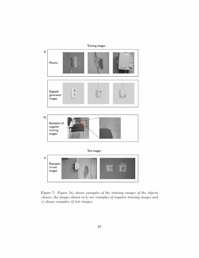
Figure 7: Figure 7a) shows examples of the training images of the objectsclasses, the images shown in b) are examples of negative training images andc) shows examples of test images.

22

4.2.1 Varying the image sizes

A part of the evaluation was to investigate how the size of the trainingimages affected the recognition results. One might expect that a low imageresolution would result in lower accuracy, since they contain less information.Using small images has the advantage that the execution time is reduced,so if the difference in performance is little, small images are preferable.

The three images sizes that are evaluated are 64x64 pixels, 80x80 pixelsand 100x100 pixels, and the size of the test images remains unchanged at400x240 pixels.

4.2.2 False positives

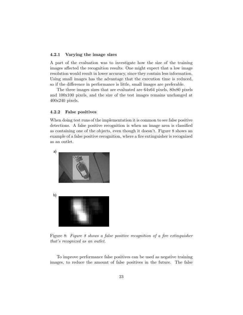
When doing test runs of the implementation it is common to see false positivedetections. A false positive recognition is when an image area is classifiedas containing one of the objects, even though it doesn’t. Figure 8 shows anexample of a false positive recognition, where a fire extinguisher is recognizedas an outlet.

Figure 8: Figure 8 shows a false positive recognition of a fire extinguisherthat’s recognized as an outlet.

To improve performance false positives can be used as negative trainingimages, to reduce the amount of false positives in the future. The false

23

positives are then divided into smaller images, and these are used as negativetraining images. In my training image set approximately 500 of the 1910images originate from false positive recognitions, identified manually.

4.3 Image scanning algorithm

The test images are searched using a sliding window approach. The sizeof the test images is 400x240 pixels, and the sliding window searching isperformed three times for each image, using the three different window sizes120x120, 80x80 and 60x60 pixels. The sliding window moves with a stepsize equal to 1/5 of the window size. This means that every area of theimage will be evaluated a number of times, and the threshold for an imagearea to be considered as containing an object is seven positive evaluations.This threshold was determined using a trial and error approach, by manuallylooking for a threshold which maximizes the number of found objects andminimizing the number of false positives.

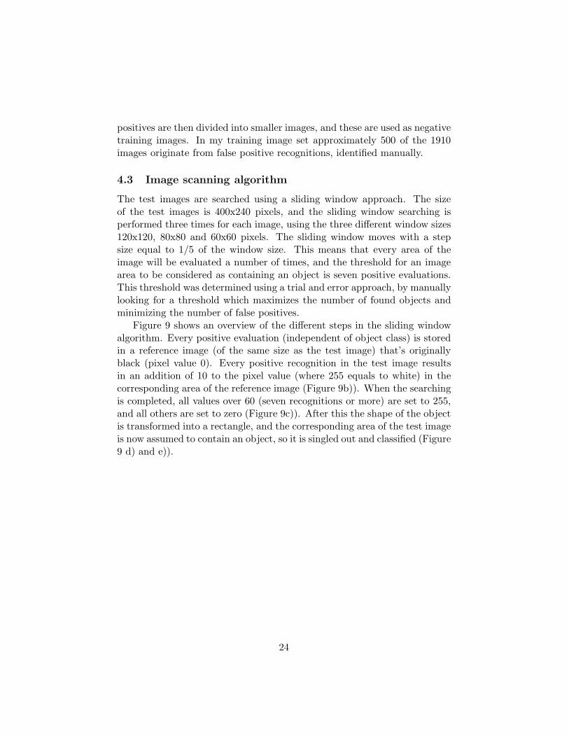
Figure 9 shows an overview of the different steps in the sliding windowalgorithm. Every positive evaluation (independent of object class) is storedin a reference image (of the same size as the test image) that’s originallyblack (pixel value 0). Every positive recognition in the test image resultsin an addition of 10 to the pixel value (where 255 equals to white) in thecorresponding area of the reference image (Figure 9b)). When the searchingis completed, all values over 60 (seven recognitions or more) are set to 255,and all others are set to zero (Figure 9c)). After this the shape of the objectis transformed into a rectangle, and the corresponding area of the test imageis now assumed to contain an object, so it is singled out and classified (Figure9 d) and e)).

24

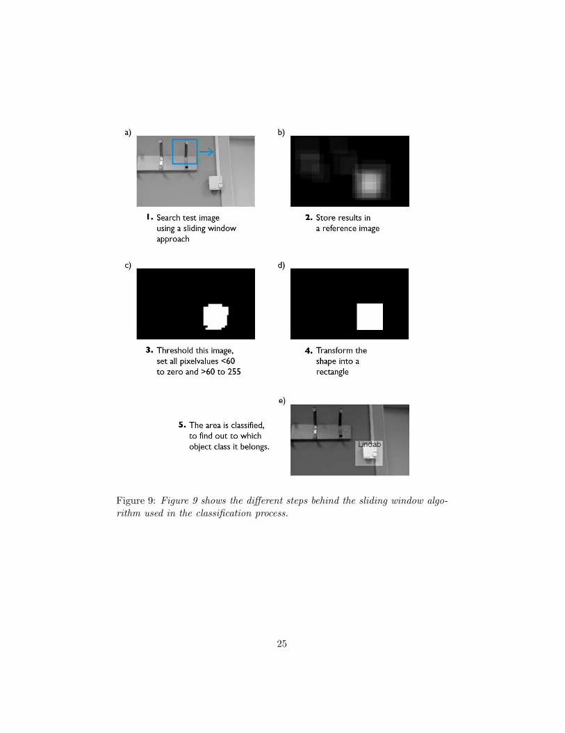
Figure 9: Figure 9 shows the different steps behind the sliding window algo-rithm used in the classification process.

25

5 Results

The performance of the implementation was evaluated by varying two pa-rameters, the size of the training images as well as testing with or withoutthe digitally generated images in the set of training images.

The performance was measured by manually looking at the output im-ages and evaluating them using a scoring system. The scoring system worksaccordingly: a correct recognition is awarded with 1 point and a correct lo-calization but with wrong object classification gives 0.5 points. The pointsare measured against the total number of points available. A false positiverecognition results in an addition of 1 point to the total number of pointsavailable in that image.

The results are presented as number of acquired points divided by thetotal number of points, in percentages.

5.1 Varying size of training images

The three training image sizes that were evaluated were 64x64 pixels, 80x80pixels and 100x100 pixels. Table 2 shows the accuracy of the performanceof the three image sizes, i.e. what proportion of the total number of pointsthey earned in each of the test images categories.

64x64 80x80 100x100 No. of ImgsEmpty 12.5% 20.0% 50% 40Outlet 53.5% 53.4% 53.7% 60LightSw 34.8% 30.1% 31.6% 60Lindab 48.8% 45.1% 41.1% 653D 35.6% 31.6% 31.1% 75

Total: 39.5% 37.9% 40.7%

Table 2: Table 2 shows the accuracy for three different sizes of the trainingimages, 64x64 pixels, 80x80 pixels and 100x100 pixels, in each of the testimage categories. The best overall performance is found in the 100x100 pixelimplementation, though the difference is small. The number of test imagesin each category is shown in the column to the right.

The 100x100 pixel implementation is overall better than the two others,with a higher performance especially for the empty class. For the otherclasses however, the 64x64 and 80x80 pixel implementations generally per-form equally good or better.

26

More specifically one can look at how many of all the objects in the testimages that were localized and correctly classified. The results are shown inTable 3.

64x64 80x80 100x100Outlet 46.1% 54.6% 52.0%LightSw 46.1% 35.7% 31.2%Lindab 43.2% 42.0% 26.0%Total: 45.1% 44.0% 36.2%

Table 3: Table 3 shows the proportion of all objects in the test images thatwere correctly localized and classified for the different sizes of the trainingimages.

Table 4 shows the number of false positive recognitions from the threeimage sizes. We see that the smaller image sizes have a higher return of falsepositives.

64x64 80x80 100x100No. of false positives 137 154 99

Table 4: Table 4 shows the number of false positive recognitions returnedfrom the three different training image sizes.

It is clear that the implementations with the smaller image sizes havea higher success rate when it comes to maximizing the number of foundobjects. The reason why their overall performance (Table 2) is slightlyworse than that of the 100x100 pixel implementation, is because they returnmore false positives. An example of this is shown in Figure 10.

27

Figure 10: Figure 10 shows the differences between the images resulting fromHOG 100x100 and HOG 64x64. HOG 64x64 finds more of the objects thanit’s counterpart, but has also a higher return of false positives.

When including the digitally rendered images in the set of training im-ages, the size of 100x100 pixels was used. Mainly because it performedslightly better overall than the other two sizes, but also because of it’s lowerreturn of false positives.

5.2 Performance when including digitally generated images

The purpose of this project was to evaluate whether it is possible to usedigitally generated images as training data for computer vision purposes.At an early stage, the possibility of using only digitally generated imagesin a set of training images was evaluated. It proved to be difficult to getpositive classification results using this approach, most likely because thelack of intraclass variability in the digitally generated images.

The main focus was then to evaluate whether or not one can add digitallyrendered images to an existing set of training images (consisting of photos) toget a higher performance. Onto the existing training set consisting of roughly200 images per class, an additional 150 digitally generated images per classwere added. All of the images were rendered from different angles, to give theas much information as possible about the objects. Two different digitally

28

rendered image sets were created, one containing the objects against a darkgrey background, and one with the objects against light gray background,and these different sets were tested separately.

The classification result were negative, in the sense that the resultingclassifications with digitally generated images included were identical to theclassifications of the original implementation (without digitally generatedimages).

The testing strategy was to evaluate the results from using the two newtraining sets (with digitally generated images included, light gray or darkgray background). The evaluation would be carried out in the same way asthe evaluation for the image sizes, measuring accuracy, correct classificationand false positives.

The results when including digitally generated images into the trainingdata set, however, were identical to the previous results. Every referenceimage (as described in Figure 9b)) was compared pixel-wise against thecorresponding image classified by the original implementation, and they didnot differ in a single pixel.

29

6 Discussion and conclusions

Some of the results of this project are unexpected, for example that thesmaller image sizes have a higher performance when it comes to correctlyfinding and classifying objects. The total performance is however slightlyworse than that for the larger images, since using the smaller image sizesleads to a higher return of false positives.

The reason for this might be because the smaller training images containless information, hence they give a less clear image of the object classes.With their less distinct image of the objects, they have a lower thresholdand will more easily give a positive output. This might be why they manageto find and correctly classify more of the objects, but also return more falsepositive recognitions.

Another unexpected result was that including digitally generated imagesin the training set didn’t change the resulting classifications at all, the imagesdisplaying the positive classifications didn’t differ in a single pixel.

The reason for this might lie in the synthetic nature of the gradientsin digitally generated images. Not only do they differ from the gradients inphotos, but they’re also very similar to each other. Therefore it doesn’t seemto matter if one adds the digitally generated images to the training data setor not, since they carry little information compared with the original dataset, in which the variability was large.

6.1 Discussions on performance

The overall performance of the implementation is quite poor. More specif-ically, it can be said that the program has a lower hit rate near the imageborders, since the sliding window algorithm will evaluate the areas in themiddle of the image more times than the areas near the border. These ef-fects might be reduced by adding a black border (˜50 pixels wide) aroundthe test images.

The runtime of the program is around a minute, which is high. Theprogram probably could be made more efficient in many ways. Except formore efficient Matlab functions (the function eval which is known to beslow, is used for its lucidity) the implementation could probably gain fromchoosing another size of the angular bins. The angle that was used was8 , and without loosing much accuracy a larger bin angle probably couldbe used (e.g. 30 or 45 ), and this would probably reduce execution timesubstantially.

Regarding the image sizes, a better classifier than the one used here

30

might be constructed by using the 64x64 or the 80x80 pixels classifier in thesliding window phase, since they have a higher return of localized objects.The 100x100 could be used in the classifying phase to decide whether theimages from the first phase are objects (as well as classifying objects) or ifthey’re empty (since the 64x64 and 80x80 classifier have a higher return offalse positives).

Regarding the possibility of adding digitally generated images to a setof training images, it is possible that digitally generated images are moreuseful when other feature descriptor methods are used, rather than HOG.The HOG descriptor takes only the gradients into account, and the gradientsin digitally generated images differ from gradients in photos. There aredescriptors that are based on other image properties than gradients, forexample the shape context feature descriptors, that are based on an object’sshape [1].

It is also possible that a better result is obtained if a higher numberof digitally generated images is used. Heisele, Kim and Meyer [12] used40,000 digitally generated images in their training data set, which consistedof digitally generated images depicting a shoe sole, an elephant, and otherobjects with distinct shapes. Here I only used 150 per class, so maybe ahigher number of these images are needed to get the same variance as whenphotos are used.

6.2 Concluding remarks

The purpose of this project was to investigate if inclusion of digitally gener-ated images as training data for an object recognition implementation couldresult in a higher performance. My findings were that including digitallygenerated images did not result in a higher performance. It is possible thatbetter result can be obtained if other descriptors than HOG are used, or ifa larger number of digitally generated training images is used.

The possibility of using digitally generated images as training imagesfor object recognition purposes is worth studying further, since the benefitswould be large. There exist many other methods of including informationfrom 3D models in object recognition schemes, but training images are stillused in many approaches and whenever this is the case, the usage of digitallygenerated images would greatly facilitate the gathering of training imagescompared to the alternative of collecting photos.

31

References

[1] S. Belongie, J. Malik & J. Puzicha,“Shape context: A new descriptor forshape matching and object recognition”, Neural Information ProcessingSystems Conference (NIPS), 2000, p. 831-837

[2] T. E. de Campos, B. Rakesh Babu, M. Varma, “Character Recognitionin Natural Images”, Computer Vision Theory and Applications (VIS-APP), 2009 International Conference on, 5-8 Feb. 2009

[3] V. Chandrasekhar, G. Takacs, D. Chen, S. Tsai, R. Grzeszczuk, B.Girod, ”CHoG: Compressed Histogram of Gradients, A Low Bit-RateFeature Descriptor”, Computer Vision and Pattern Recognition, 2009.CVPR 2009. IEEE Conference on, 25-29 June 2009, p. 2504-2511

[4] Y. Cheng, “Vision-Based Online Process Control in Manufacturing Ap-plications”, Automation Science and Engineering, IEEE Transactionson, Jan. 2008, p. 140-153 vol. 5 Issue: 1

[5] C. Cortes, V. Vapnik, “Support-vector networks”, Machine Learning,Volume 20, Issue 3, Sept. 1995, p. 273-297

[6] N. Dalal, B. Triggs, ”Histograms of Oriented Gradients for Human De-tection”, Computer Vision and Pattern Recognition, 2005. CVPR 2005.IEEE Conference on, 25 June 2005, p. 886-893 vol. 1

[7] M. F. Doustar, HOG. URL http://farshbafdoustar.blogspot.se/2011/09/hog-with-matlab-implementation.html

[8] D. A. Forsyth, J. Ponce, “Computer Vision - A Modern Approach”, 2ndEdition, Pearson Education Limited, 2012, Essex (ISBN 0-273-76414-4)

[9] Y. Freund, R. E. Schapire, ”A decisiontheoretic generalization of on-line learning and an application to boosting”, Computational LearningTheory, Second European Conference, EuroCOLT ’95 Barcelona, 13-15March 1995, p. 23-37

[10] M. A. Garcia-Garrido, M. A. Sotelo, E. Martın-Gorostiza, “Fast RoadSign Detection Using Hough Transform for Assisted Driving of Road Ve-hicles”, Computer Aided Systems Theory – EUROCAST 2005, 10th In-ternational Conference on Computer Aided Systems Theory, vol. 3643,7-11 Feb. 2005, p. 543-548

32

[11] R. C. Gonzales, R. E. Woods, “Digital Image Processing”, 3rd Edition,Pearson Education Inc., 2008, New Jersey (ISBN 0-13-505267-X)

[12] I. Gordon, D. G. Lowe, ”What and Where: 3D Object Recognition withAccurate Pose”, Lecture Notes in Computer Science, Volume 4170/2006,2006

[13] B. Heisele, G. Kim, A.J. Meyer, ”Object Recognition with 3D Models”,British Machine Vision Conference, 2009

[14] J. Liebelt, C. Schmid, ”Multi-View Object Class Detection with a 3DGeometric Model”, Computer Vision and Pattern Recognition, 2010.CVPR 2010. 23rd IEEE Conference on, Dec 2010, p. 1688-1695

[15] J. Liebelt, C. Schmid, K. Schertler, ”Viewpoint-Independent ObjectClass Detection using 3D Feature Maps”, Computer Vision and PatternRecognition, 2008. CVPR 2008. IEEE Conference on, 23-28 June 2008,p. 1-8

[16] J. C. Liter, H. H. Bulthoff, “An Introduction To Object Recognition”,Z. Naturforsch. 53c, March 1998, p. 610-621

[17] D. G. Lowe, ”Object Recognition From Local Scale-Invariant Features”,Proceedings of the 7th IEEE International Conference on ComputerVision, 1999, p. 1150-1157

[18] M. Stark, M. Goesele, B. Schiele, ”Back to the Future: Learning ShapeModels from 3D CAD Data”, British Machine Vision Conference, 2010

[19] Q. Zhu, S. Avidan, M-C Yeh, K-T Cheng, “Fast Human Detection Us-ing a Cascade of Histograms of Oriented Gradients”, Computer Visionand Pattern Recognition, 2006 IEEE Computer Society Conference on,2006, p. 1491-1498

[20] X. Zhu, C. Vondrick, D. Ramanan, C. Fowlkes, ”Do We Need MoreTraining Data or Better Models for Object Detection?”, British Ma-chine Vision Conference (BMVC), 2012

[21] M. Z. Zia, M. Stark, B. Schiele, K. Schindler, ”Revisiting 3D Geomet-ric Models for Accurate Object Shape and Pose”, Computer VisionWorkshops (ICCV Workshops), 2011 IEEE International Conferenceon, 6-13 Nov. 2011, p. 569-576

33