Object-Oriented Implementation of LTE Turbo Codes - …wvuscholar.wvu.edu/reports/Gangadi_Anusha.pdf · Abstract Object-Oriented Implementation of LTE Turbo Codes by Anusha Gangadi

Object-Oriented Implementation of LTE

Turbo Codes

by

Anusha Gangadi

Problem Report submitted to theCollege of Engineering and Mineral Resources

at West Virginia Universityin partial fulfillment of the requirements

for the degree of

Master of Sciencein

Electrical Engineering

Vinod Kulathumani, Ph.D.Xin Li, Ph.D.

Matthew C. Valenti, Ph.D., Chair

Lane Department of Computer Science and Electrical Engineering

Morgantown, West Virginia2010

Keywords: Digital Modulation, Object-Oriented Programming, Turbo Codes

Copyright 2010 Anusha Gangadi

Abstract

Object-Oriented Implementation of LTE Turbo Codes

by

Anusha GangadiMaster of Science in Electrical Engineering

West Virginia University

Matthew C. Valenti, Ph.D., Chair

Turbo codes are a popular form of error correction codes as they perform close to theShannon limit. Turbo codes have interesting features like parallel code concatenation, non-uniform interleaving, and an iterative decoding algorithm. Because of these features, turbocodes are adopted by various standards like NASA’s for deep space communications, thirdgeneration cellular standards like UMTS and cdma2000, and the latest mobile network tech-nology called 3GPP LTE (Long Term Evolution). The main objective of this problem reportis to study the implementation and behavior of the LTE turbo codes. An object-orientedapproach is considered for the implementation of the turbo codes. To achieve the objectivesof this report, a previously developed library called the Coded Modulation Library (CML),which was developed at West Virginia University’s Wireless Communications Research Lab-oratory (WCRL), is extended to support the turbo codes specified in the LTE standard inan object-oriented fashion.

This report begins with a brief overview of communication and coding theory, and dis-cusses the use of object-oriented programming for simulating communication systems. Next,a clear study of convolutional and turbo codes is presented, including a discussion of theencoding and decoding of the codes. An object-oriented Matlab implementation of LTETurbo codes is also discussed in detail. Simulation results are obtained using the LTE turbocode class developed in this report along with a class from Matlab’s Communication Toolboxcalled the Error Rate Test Console. Results are shown that illustrate the influence of keyparameters such as codeword length and the choice of decoding algorithm.

iii

Acknowledgements

I would like to heartily thank my committee chair and advisor, Dr.Matthew C. Valenti,

for giving me the opportunity and encouragement to work with him. This problem report

became easier with his constant guidance and support, apart from developing good under-

standing of the subject.

I would also like to thank Dr.Vinod Kulathumani and Dr.Xin Li. I am fortunate enough

to have the opportunity to take courses with all of my committee members, and therefore my

course work became helpful for the problem report. I would like to thank to my colleague,

Mohammad Fanaei for helping me understand the working of CML2 and the relation between

CML and CML2.

Lastly, I also thank my family, friends and offer my regards to all of those who supported

me in any respect during the completion of the project.

iv

Contents

Acknowledgements iii

List of Figures vi

List of Tables vii

1 Introduction 11.1 Evolution of Cellular Systems . . . . . . . . . . . . . . . . . . . . . . . . . . 11.2 Importance of Turbo Codes . . . . . . . . . . . . . . . . . . . . . . . . . . . 31.3 System Model . . . . . . . . . . . . . . . . . . . . . . . . . . . . . . . . . . . 4

1.3.1 BPSK Modulation . . . . . . . . . . . . . . . . . . . . . . . . . . . . 51.3.2 Log Likelihood Ratio . . . . . . . . . . . . . . . . . . . . . . . . . . . 5

1.4 Basic Coding Theory . . . . . . . . . . . . . . . . . . . . . . . . . . . . . . . 51.4.1 Convolutional Codes . . . . . . . . . . . . . . . . . . . . . . . . . . . 61.4.2 Turbo Codes . . . . . . . . . . . . . . . . . . . . . . . . . . . . . . . 7

1.5 Object-Oriented Simulation . . . . . . . . . . . . . . . . . . . . . . . . . . . 71.6 Outline of Report . . . . . . . . . . . . . . . . . . . . . . . . . . . . . . . . . 9

2 Convolutional Codes 102.1 Convolutional Encoding . . . . . . . . . . . . . . . . . . . . . . . . . . . . . 11

2.1.1 Encoder Diagram . . . . . . . . . . . . . . . . . . . . . . . . . . . . . 112.1.2 State Diagram . . . . . . . . . . . . . . . . . . . . . . . . . . . . . . . 122.1.3 Trellis Representation . . . . . . . . . . . . . . . . . . . . . . . . . . 13

2.2 Decoding Algorithm . . . . . . . . . . . . . . . . . . . . . . . . . . . . . . . 132.2.1 Viterbi Algorithm . . . . . . . . . . . . . . . . . . . . . . . . . . . . . 142.2.2 SISO Decoding . . . . . . . . . . . . . . . . . . . . . . . . . . . . . . 142.2.3 RSC Codes . . . . . . . . . . . . . . . . . . . . . . . . . . . . . . . . 15

2.3 Matlab Implementation . . . . . . . . . . . . . . . . . . . . . . . . . . . . . . 16

3 Turbo Codes 193.1 PCCC Encoder . . . . . . . . . . . . . . . . . . . . . . . . . . . . . . . . . . 193.2 Interleaving . . . . . . . . . . . . . . . . . . . . . . . . . . . . . . . . . . . . 203.3 Decoding . . . . . . . . . . . . . . . . . . . . . . . . . . . . . . . . . . . . . . 213.4 Matlab Implementation . . . . . . . . . . . . . . . . . . . . . . . . . . . . . . 22

CONTENTS v

4 Results 244.1 Error Rate Test Console . . . . . . . . . . . . . . . . . . . . . . . . . . . . . 244.2 Performance Curves . . . . . . . . . . . . . . . . . . . . . . . . . . . . . . . . 26

5 Conclusion 30

References 32

vi

List of Figures

1.1 Growth in cellular subscribers in the United States [Source: ctia.org]. . . . . 31.2 System model representation. . . . . . . . . . . . . . . . . . . . . . . . . . . 4

2.1 Encoder for (2,1,2) convolutional code . . . . . . . . . . . . . . . . . . . . . 112.2 Encoder diagram for NSC codes. . . . . . . . . . . . . . . . . . . . . . . . . 122.3 State diagram representation for NSC codes. [Figures used from class notes

with the permission of Dr. M.C.Valenti] . . . . . . . . . . . . . . . . . . . . 122.4 Encoding using trellis representation . . . . . . . . . . . . . . . . . . . . . . 132.5 Explanation of Viterbi algorithm . . . . . . . . . . . . . . . . . . . . . . . . 152.6 RSC encoder . . . . . . . . . . . . . . . . . . . . . . . . . . . . . . . . . . . 162.7 State diagram representation for RSC codes . . . . . . . . . . . . . . . . . . 162.8 Encoding using trellis representation for RSC codes . . . . . . . . . . . . . . 17

3.1 Block diagram of turbo encoder. . . . . . . . . . . . . . . . . . . . . . . . . . 203.2 Block diagram of turbo decoder. . . . . . . . . . . . . . . . . . . . . . . . . . 22

4.1 Performance of the datalength 6144 LTE turbo code for different decoderiterations. BPSK modulation and AWGN channel is considered. . . . . . . . 27

4.2 Bit Error performance of LTE Turbo system for different datalengths. . . . . 284.3 Plot showing the performance of the datalength 6144 LTE turbo code for

different decoder types. . . . . . . . . . . . . . . . . . . . . . . . . . . . . . . 29

vii

List of Tables

3.1 Turbo code internal interleaver parameters. . . . . . . . . . . . . . . . . . . 21

1

Chapter 1

Introduction

From the day that cell phones first became adopted to the present day, there have been

many improvements in the field of cellular systems. Cell phones have become a necessary

device in our lives. Before going into the details of the turbo codes used in the Long Term

Evolution (LTE) cellular standard and their features, this chapter begins with a discussion

of the evolution of cellular systems. Later, the basic system model used throughout this

report is presented along with a review of basic terminology used in the report. A brief

overview is given on the topics of communication theory, coding theory, and object-oriented

programming. Finally, the chapter concludes with an outline of remainder of the report.

1.1 Evolution of Cellular Systems

The history of mobile phones began with two-way radios and continues through the

emergence of modern mobile phones. Early development of mobile phones started in the

1920’s making use of radio telephones. Radio telephones were first introduced in passenger

trains in Europe in 1926. From 1940’s, the development took a shape by introducing a

two-ray radio called “walkie-talkie”. After this, an improvement was made to the two-way

radio and successfully, a radio mobile phone was mounted inside a car. This device was able

to connect to a local telephone network for a range of 20 kilometers. The mobile phones

developed during the early years were serviced by one base station throughout the phone

call, which means they had no continuity of service as the phones moved out of range of the

Anusha G Chapter 1. Introduction 2

base station. The first fully automated mobile phone system for vehicles was introduced in

Sweden in 1960 and was named as MTA (Mobile Telephone system A). It allowed and received

calls using a rotary dial system. Later, an upgraded version called MTB (Mobile system B)

was introduced which uses push-button dial system. In this, outgoing calls could be dialed

directly but incoming calls had to be operated by a person to detect the base station of

the arriving call. In 1970’s, Bell Laboratory introduced an automatic “call handoff” system

which allowed mobile phones to move through several cell areas without stoppage. Handheld

cell phone was first introduced by Motorola researchers, which from then evolved into a huge

success. The concepts of frequency reuse and handoff were introduced in modern cell phone

technology.

Mobile phone history is divided into generations like 1G, 2G and 3G to reflect the de-

velopments in mobile technology. Coming to the first generation (1G) mobile phones, the

main development was in the use of multiple cell sites and the ability to transfer from one

cell site to another cell site during a conversation without any interruption. In the second

generation (2G), mobile phone systems emerged, primarily using the GSM standard and the

2G phone systems differ from the first generation in the use of digital transmission instead

of analog transmission and also by the introduction of advanced and fast phone-to-network

signaling. Starting with 2G, new tiny hand held phones were introduced. 2G introduced a

new communication system called SMS or text messaging. 2G also introduced the ability to

access media content on mobile phones.

In the third generation (3G), the main technological difference is the use of packet switch-

ing rather than circuit switching for data transmission. 2.5G systems such as CDMA2000 and

GPRS were developed while 3G was in the process of being deployed, and these provide 3G

features without fulfilling the promised high data rates or full range of multimedia services.

For the first time, media streaming of radio (and even television) content is introduced using

the high connection speeds of 3G technology [1]. In 2009, fourth generation (4G) came into

the picture to improve the speed improvements up to 10-fold over existing 3G technologies.

The first two commercially available technologies billed as 4G are the WiMAX standard and

the LTE standard. In 4G, circuit switching is eliminated and replaced by an all-IP network.

Thus, 4G provides voice calls just like any other type of streaming audio media, utilizing


Figure 1.1: Growth in cellular subscribers in the United States [Source: ctia.org].

packet switching over the Internet, LAN or WAN networks via VoIP [2]. According to the

latest information, West Virginia will be on the edge of using 4G LTE wireless networks, as

Verizon has announced that they will be launching 4G LTE wireless networks in Charleston,

WV [3].

In recent years, wireless and cellular technology has seen remarkable improvements re-

sulting in an increasing number of mobile phones [4]. Cellular/digital technology has gained

market share, as a result of the increased demand for notebook, computers and smart mobile

phones. The growth of cellular subscribers is shown in the Fig. 1.1 which plots the number

of subscribers in the United States against the year. The graph also shows that the growth

of cellular subscribers in the United States has drastically increased from year 1995 to year

2009. In a span of 10 yrs, the rate has increased approximately to 8 times 1.

1.2 Importance of Turbo Codes

Turbo codes are a special class of codes which have extraordinary performance at low

SNR. They have energy efficiencies very close to the Shannon limit [5]. Turbo codes have

special features like parallel code concatenation, non-uniform interleaving, recursive con-

volutional encoding, and an iterative decoding algorithm. Besides this, turbo codes have

achieved improvement in interleaver gain by obtaining low weight code words. Unlike tradi-

1ctia.org


Figure 1.2: System model representation.

tional (e.g. block) interleavers, the interleavers used by turbo codes permute the data in a

pseudo-random fashion, which allows the code to produce mostly low-weight code words.

Turbo codes are used in many applications. Turbo codes allow for relatively high data

rates. They are mainly intended for satellite communications, wireless internet access, wire-

less local area networks (LAN’s), microwave systems, and mobile communications applica-

tions. Specific standards that use turbo codes include CCSDS (for deep-space communica-

tions), mobile communications like UMTS and CDMA2000 (3G mobile), satellite telecom-

munications like DVB-RCS (return channel over satellite), DVB-RCT (return channel over

terrestrial), Inmarsat (M4) and Eutelsat (Skyplex), wireless Internet access like IEEE 802.16

(Wimax), LTE [6].

1.3 System Model

The system model shown in Fig. 1.2 is presented to describe the concept of digital

communications [7]. The signal s(t) is drawn from a set S consisting of “M” different

signals, which are passed through the channel. The n(t) represents the white Gaussian noise

of the channel. The received signal, r(t) is the sum of the signal and the noise [8].


1.3.1 BPSK Modulation

A popular method of transmitting information using two bits is called Binary Phase Shift

Keying (BPSK). Two symbols s1 and s2 are used to represent BPSK modulation. With

BPSK modulation, a single bit is used to select from among the two possible symbols. We

vary the phase of the signal to transmit information. When represented as a 2-dimensional

signal-space diagram, a BPSK signal lies in the same axis, either x-axis or y-axis and every

bit transitions the signal by 180 degree phase shift.

1.3.2 Log Likelihood Ratio

Turbo codes use soft-decision decoding and require log-likelihood ratio (LLR) as the

input to the decoder. The equation of the LLR is given as,

λi = logP [ci = 1 | ri]P [ci = 0 | ri]

(1.1)

where ci is the ith transmitted code bit and ri is the discrete-time representation of the signal

received during the ith signalling interval.

For BPSK modulation in an additive white Gaussian noise (AWGN) channel, the LLR

may be expressed as

λi =2

σ2· ri (1.2)

where ri is the received signal and σ2 is the variance of the additive white Gaussian noise.

1.4 Basic Coding Theory

Some basic terms related to coding theory are defined here, which are helpful in the

following chapters.

• Linear Codes: A code is said to be linear if it contains the all-zeros code word and the

sum of any two code words is also a code word.


• Generator Matrix: For a linear code, the codeword is given by c = Gu, where u is the

k-bit message, c is the n-bit codeword, and G is the k by n bit generator matrix.

• Hamming Distance: The Hamming distance between any two code words is defined

as the number of positions they differ. The Hamming distance d(ci, cj) is calculated

by taking the difference, nothing but calculating the modulo-2 sum between the code

words and finding the weight.

• Minimum Hamming distance: The minimum hamming distance is the smallest ham-

ming distance of all the code words.

• Systematic Codes: A code is called a systematic code only if the code words can be

expressed as c = (u,p) where u is the message and p is the parity information. The

generator matrix for systematic codes is given as,

G = [IkP ],

where Ik is the identity matrix of size k by k and P is a matrix of size k by (n− k).

• Cyclic Codes: A code C is said to be cyclic if every cyclic shift of the codeword is also

a codeword in C. A cyclic code can be characterized by a polynomial of degree (n− k)

called the generator polynomial.

1.4.1 Convolutional Codes

Due to the poor performance of cyclic codes near low SNR, convolutional codes are in-

troduced. Convolutional codes are a generalization of the cyclic codes. Convolutional codes

are formed with more than one generator ploynomial to operate at low rates. Convolutional

codes are popular as they are applied to satellite, deep space communication and mobile

communications like CdmaONE, GSM. Also UMTS uses convolutional codes. Convolu-

tional codes are classified as either non-systematic convolutional (NSC) codes or recursive

systematic convolutional (RSC) codes. The difference between these two categories of con-

volutional codes is that with an RSC code, the output of one of the generators is fed back

to the input [9].


1.4.2 Turbo Codes

Turbo codes are a recent development. Turbo codes are formed by concatenation of

two or more basic codes. Usually, RSC codes are used as constituent codes. The turbo

codes make use of these features: parallel concatenation of codes to allow simpler decoding;

non-uniform interleaving to provide better weight distribution; and soft decoding to enhance

decoder decisions. Turbo codes are used in many commercial applications, including both

third generation cellular systems UMTS and cdma2000.

1.5 Object-Oriented Simulation

Researchers at WVU Wireless Communications Research Lab (WCRL) have developed

an open-source simulator which runs in Matlab called the Coded Modulation Library (CML).

Now, a second generation of CML called CML2 is being developed which is an object-oriented

version of CML. A key benefit of object-oriented programming is that it gives the user the

flexibility to rapidly introduce new functionality. The purpose of this problem report is to

evaluate the flexibility of CML2 by implementing the LTE turbo codes in an object-oriented

fashion [10].

Object-oriented programming (OOP) is a programming technique organized completely

with “objects” rather than “actions”. Object-oriented programming is all about classes and

objects. This reduces the task of creating the same function or method every time we want to

use them, by specifying all the properties and methods (together called as members) in one

class. If we want to use the properties and methods of a particular class, we just create any

number of objects for that class or we can inherit the properties or methods of the class in

our own class. This makes the object-oriented programming simple and easy to understand.

A class is a template for an object, a user-defined data type that contains variables,

properties and methods. A Matlab class is described by a file containing the following

segments:

Classdef classname (demo)

properties;


methods;

end

To list the properties or methods of a particular class, we can use the following command

in Matlab,

Properties(classname);

Methods(classname);

An object created at the run-time is nothing but an instance of a class. The object

consists of the state and behavior that is defined in the class. In Matlab, we can create an

object as shown below. An object “A” of class demo is created.

A = demo;

Object-oriented programming is often used because of the following reasons.

• We can define sub-classes for existing classes (called a superclass), with the concept

called inheritance. This becomes useful when we want to reuse a definition to define a

more specific sub category.

• We can specify static methods to define an operation for the class.

• We can use handle classes with reference behavior, making data structures like linked

lists.

• Lastly, “Overloading” is a concept where we can define existing Matlab functions to use

on our object by just providing a function with that name in our methods. Overloading

is not only for functions/methods, it can also used be with the operators. Example for

overloading a function can be use of “plot” function.


1.6 Outline of Report

The purpose of this problem report is to study the object-oriented CML. Making use of

CML, we want to analyze the behavior of LTE Turbo codes for various data lengths and

different number of decoder iterations by generating plots for both. In this chapter, we

have discussed a digital communications system and have provided a brief description of the

terms required in the following chapters. For more detailed explanations concerning digital

communications systems, the reader is encouraged to refer to [11, 12]. In addition, a study

of using object oriented programming has been presented.

In Chapter 2, a detailed discussion of convolutional codes, the types, and encoding and

decoding of the convolutional codes is presented. This discussion helps in implementing the

convolutional codes in CML2. Moving to the Chapter 3, turbo codes, interleaver used in

turbo codes, encoding and decoding of the turbo codes is discussed. Furthermore, Matlab

implementation of turbo codes in CML2 is depicted clearly. Finally in Chapter 4, the usage

and functioning of error rate test console with inclusion of final plots is presented.

10

Chapter 2

Convolutional Codes

Convolutional codes are a generalization of the cyclic codes. Convolutional codes

introduce redundant bits into the data stream through the use of linear shift registers. A

convolutional encoder is a device with k inputs and n outputs, where n ≥ k. Convolutional

encoders are characterized by the following three parameters.

• k is the number of input bits

• n is the number of output bits and

• m is the memory of the encoder

The code rate r is defined as r = k/n. It gives a measure of the efficiency of the code.

The constraint length, K for a convolutional code is defined as K = 1 + m, where m is

the memory size. The shift registers store the state of the convolutional encoder and the

constraint length relates the number of bits upon which the output depends.

A simple example is illustrated to understand the convolutional encoder. From Fig. 2.1, a

square box is used for linear shift registers and also an assumption is made that the encoders

are initiated with 0’s in the shift registers. Each new data bit is shifted into the shift register,

and an encoded bit is produced at the encoder’s output. This is a simultaneous process and

likewise, this process repeats untill all the bits are encoded. Finally, the output will be a

linear combination of the contents of the shift register [11].

The number of memory elements in Fig. 2.1 is 2, therefore the constraint length, K = 1+

2 = 3. The output c(1) is obtained by adding the input message bit u to the contents of both

Anusha G Chapter 2. Convolutional Codes 11

u

D D

c(0)

c(1)

Figure 2.1: Encoder for (2,1,2) convolutional code

elements of the shift register. On the other hand, the output c(0) is obtained by adding the

input message bit u to the content of just the second element of the shift register. From this

information, we can represent the generators in the binary form as G(1) = [111], G(0) = [101].

2.1 Convolutional Encoding

Convolutional encoders are formed using shift registers and modulo-2 registers, where

outputs are the modulo-2 sum of selective shift register contents and input bits. The infor-

mation bits are given as input to the shift registers and the output encoded bits are obtained

by modulo-2 addition (XOR) of the input information bits and the values contained in the

shift registers.

2.1.1 Encoder Diagram

An encoder is represented by delay elements and exclusive-or gates. The encoder can

be formed from the information of the generators and for (5,7) generators, two memory

elements are required. Binary representation of (5,7) generators is given as, G(0) = 101 and

G(1) = 111 illustrated in the Fig. 2.2.


u

D D

c(0)

c(1)

Figure 2.2: Encoder diagram for NSC codes.

Figure 2.3: State diagram representation for NSC codes. [Figures used from class notes withthe permission of Dr. M.C.Valenti]

2.1.2 State Diagram

A state diagram is used to give the description of the system by representing all the

possible states of a convolutional encoder. The number of states in the state diagram depends

on the memory registers and is equal to 2m, where m is the number of shift registers and the

contents of the shift registers represent the states. The output depends on all the possible

states of the delays and each input [13]. For the example given by Fig. 2.2, the state diagram

is represented as shown in Fig. 2.3.

A state diagram is formed by drawing a graph, and nodes in the encoder diagram repre-

sent all possible states. Each state is labeled with a transition as uc(0)c(1)

where u denotes the

input bits and c(0), c(1) denotes output bits.


Figure 2.4: Encoding using trellis representation

2.1.3 Trellis Representation

A trellis is a graphical representation in which the nodes are ordered in terms of time,

where nodes in the trellis diagram represent the states, and the transitions are represented

by input and possible outputs for that particular input. In general, the trellis starts in the

all-zeros state and ends in the all-zeros state. Termination in the all-zeros state requires a

tail of m zeros. From the trellis in Fig. 2.4, it is clear that for any input, the sequence of

state transitions, inputs and outputs of the encoder is represented as a path.

Encoding can be performed using trellis diagram. With the message bits, we can track

the corresponding output bits. This forms the codeword.

2.2 Decoding Algorithm

Though many decoding algorithms have been developed, the Viterbi algorithm is the

most popular and widely used algorithm. The Viterbi algorithm produces hard outputs

whereas soft-in-soft-out (SISO) decoder produces soft outputs, which is more important

while working with turbo codes.


2.2.1 Viterbi Algorithm

The Viterbi algorithm is the optimum algorithm used to decode convolutional codes.

There are simplifications to reduce the computational load. They rely on searching only the

most likely paths. Viterbi algorithm is mainly designed to reduce the complexity. There

are two ways to decode using Viterbi algorithm, hard-decision decoding and soft-decision

decoding.

In hard-decision decoding, firstly a forward sweep through the trellis is performed. The

received bits are compared with the output bits and difference is stored at each node. After

which, a branch metric is computed for every branch and the least is considered. At each

node, an add, compare, and select (ACS) operation is performed. This continues until the

last node is reached. Once the end of the trellis is reached a trace back operation is performed.

During this trace back operation, the message bits are obtained.

In soft-decision decoding, the input to the decoder is the log likelihood ratios (LLRs),

which are computed using the equation 1.2. The received bits are multiplied with LLR’s

and now they are compared with the output bits and the difference is stored at each node.

A branch metric is computed for every branch and the largest is considered. At each node

point add, compare and select operation is performed. Thus in soft-decision, the larger

branch metric is selected instead of the smaller one. This is explained in Fig. 2.5. The value

at each node is calculated using,

αk = max [(αi + γi,k) , (αj + γj,k)]] (2.1)

where αi, αj represents the node which holds a partial path metric at present level and αk

represents the node value at next level. γi,k and γj,k represent the branch metric. The LLR

value calculated here, is used in soft-decision decoding. For calculating the branch metric,

first the codeword is multiplied with the LLR value at each and every branch.

2.2.2 SISO Decoding

A soft-input, soft-output(SISO) decoder updates the LLR’s of the code bits and message

bits based on the forward sweep through trellis and backward sweep through trellis. Because


i,k

10

i

j

k

j,k

Figure 2.5: Explanation of Viterbi algorithm

of the two sweeps, SISO decoding is more complex compared to viterbi decoding. The

equation (2.1) is modified by considering max ∗ in the place of max.

αk′

= max ∗ [(αi + γi,k) , (αj + γj,k)] (2.2)

where

max ∗[x, y] = log(ex + ey)

= max[x, y] + log(1 + e−|y−x|

)︸︷︷︸

fc(|y−x|)

(2.3)

Here, fc(|y − x|) is the correction function and if the correction function is a straight

line, then the algorithm is called linear-log-MAP. The equation 2.3 can be approximated as

max ∗[x, y] ≈ max[x, y] (2.4)

If this approximation is used, the algorithm is called the max-log-MAP algorithm.

2.2.3 RSC Codes

Turbo codes use recursive systematic convolutional (RSC) codes. An RSC code is very

much similar to NSC code, except that one of the output in RSC codes is the same as the

input bits. An RSC code may be constructed from a standard convolutional encoder by

feeding back one of the outputs. The feedback of one output allows one of the outputs to be

the input, hence it is systematic. The RSC encoder is shown in Fig. 2.6.


Figure 2.6: RSC encoder

Figure 2.7: State diagram representation for RSC codes

The state diagram and the trellis are identical to that of an NSC code, except that some

input labels have been reversed. The state diagram and trellis representation for NSC codes

are shown in Fig. 2.7 and Fig. 2.8 respectively.

2.3 Matlab Implementation

In this section, we will illustrate how to encode and decode a convolutional code in

CML2. First a “ConvCode” object must be created, which is accomplished with the following

command:

A = ConvCode([1 0 1 1]);


Figure 2.8: Encoding using trellis representation for RSC codes

Having entered this command, there is now an object called ‘A’ of class “ConvCode” in

the Matlab workspace. Next, we need to create some random binary data:

msg = randi([0 1],1,40,’uint8’);

The vector ‘msg’ is a length-40 vector of random binary data. Notice that it needs to be

of type ‘uint8’, which is a 1-byte character. Using a 1-byte character reduces the amount of

memory used by Matlab, since otherwise Matlab will default to a double-precision floating

point number, which is not necessary to represent a bit. Now that we have the message bits,

we need to encode the message bits using the “Encode” method.

Code = A.Encode(msg);

Now, the vector variable ‘Code’ contains the encoded bits. We are using BPSK modula-

tion, so BPSK modulation is performed.

mod = 2*Code - 1;

Random noise is added to the modulated codeword, where ‘var’ is the variance calculated

from EsNo which is the symbol energy per noise ratio. Now, let us introduce random noise

into the modulated data:

r = mod + (1/sqrt(var))*randn(size(Code));


Since we are using soft-decision decoding, we are generating log-liklehood ratio using the

formula, llr =2 ∗ codeσ2

.

llr = 4*r;

Now, the llr’s obtained are used as inputs in for the “Decode” method of class “Con-

vCode”.

out = A.Decode(llr);

Having decoded the msg, next we need to find the number of errors. beginverbatim

NumErrors = A.NumError

From the properties of ConvCode class, NumError property is used to find the number

of errors. The number of errors obtained by using NumError is shown below.

NumErrors =

0

19

Chapter 3

Turbo Codes

A turbo code is formed by concatenating two or more basic codes [14]. These basic

codes can be convolutional codes or block codes. As we are referring to the turbo codes used

in LTE, the two codes used are RSC convolutional codes. These two codes are seperated by

an interleaver to reorder the data at the input of the different encoders. Interleavers used

in turbo codes are different from the traditional interleavers in a way that turbo code inter-

leavers rearrange the order of the data bits in a pseudo random manner. The decoding is an

iterative process. There is a constituent decoder for each constituent code. The constituent

decoders are soft-in-soft-out (SISO) decoding type. The decoders exchange information after

every iteration and the iterations proceed until either data is correct or a maximum number

of iterations are reached.

3.1 PCCC Encoder

The turbo code discussed here is used by the long term evolution (LTE) specification,

as standardized by the Third-Generation Partnership Project (3GPP) [15]. The scheme

of turbo encoder is a Parallel Concatenated Convolutional Code (PCCC) with two 8-state

constituent encoders and one turbo code internal interleaver. The coding rate of turbo

encoder is 1/3. The structure of turbo encoder is shown in Fig. 3.1.

A turbo encoder is a parallel concatenation of two codes. The two codes used are RSC

Codes which are dicussed in chapter 2. As the two codes work parallely on the input data,

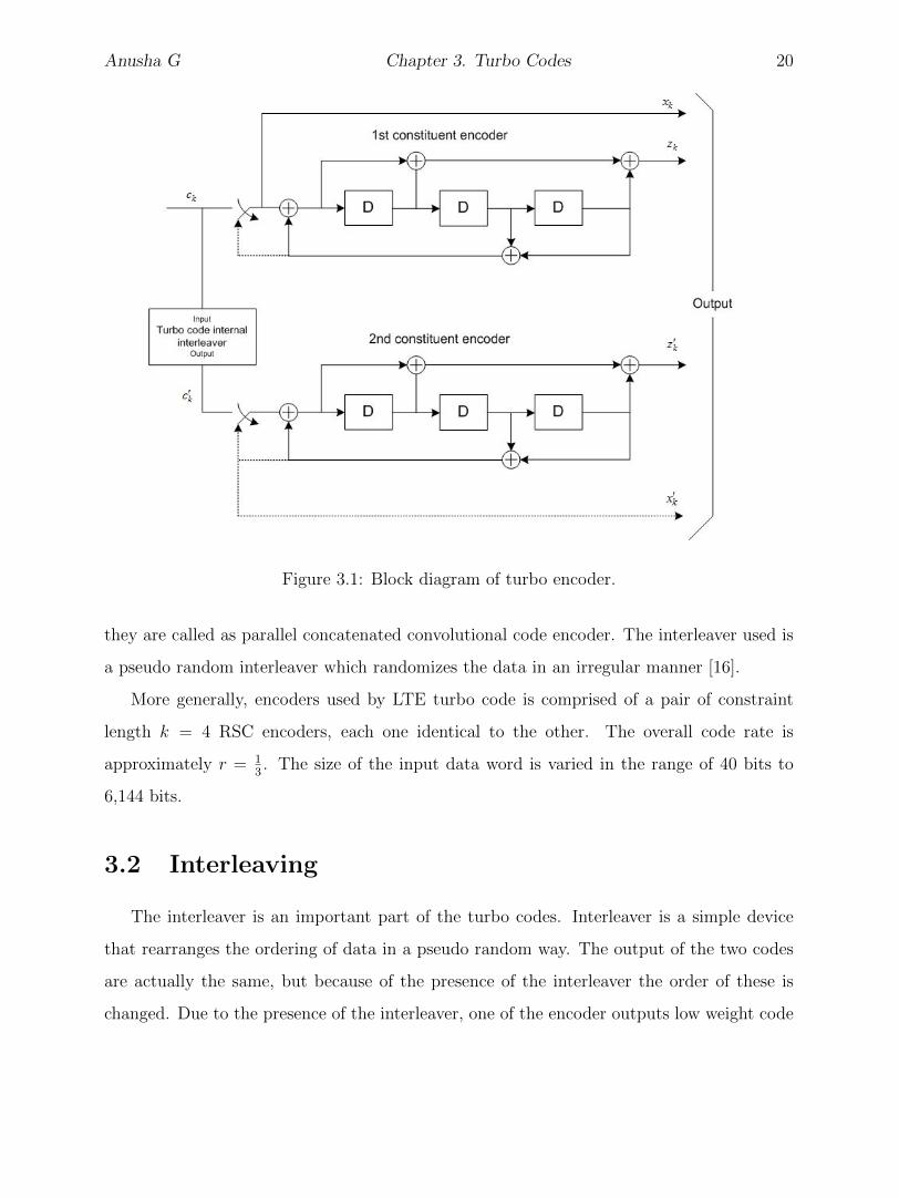
Anusha G Chapter 3. Turbo Codes 20

Figure 3.1: Block diagram of turbo encoder.

they are called as parallel concatenated convolutional code encoder. The interleaver used is

a pseudo random interleaver which randomizes the data in an irregular manner [16].

More generally, encoders used by LTE turbo code is comprised of a pair of constraint

length k = 4 RSC encoders, each one identical to the other. The overall code rate is

approximately r = 13. The size of the input data word is varied in the range of 40 bits to

6,144 bits.

3.2 Interleaving

The interleaver is an important part of the turbo codes. Interleaver is a simple device

that rearranges the ordering of data in a pseudo random way. The output of the two codes

are actually the same, but because of the presence of the interleaver the order of these is

changed. Due to the presence of the interleaver, one of the encoder outputs low weight code


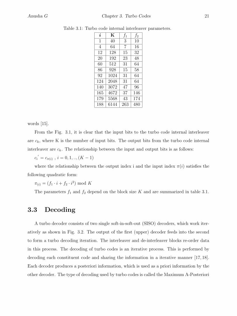
Table 3.1: Turbo code internal interleaver parameters.

i K f1 f21 40 3 104 64 7 1612 128 15 3220 192 23 4860 512 31 6486 928 15 5892 1024 31 64124 2048 31 64140 3072 47 96165 4672 37 146179 5568 43 174188 6144 263 480

words [15].

From the Fig. 3.1, it is clear that the input bits to the turbo code internal interleaver

are ck, where K is the number of input bits. The output bits from the turbo code internal

interleaver are ck . The relationship between the input and output bits is as follows:

ci′= cπ(i) , i = 0, 1, .., (K − 1)

where the relationship between the output index i and the input index π(i) satisfies the

following quadratic form:

π(i) = (f1 · i+ f2 · i2) mod K

The parameters f1 and f2 depend on the block size K and are summarized in table 3.1.

3.3 Decoding

A turbo decoder consists of two single soft-in-soft-out (SISO) decoders, which work iter-

atively as shown in Fig. 3.2. The output of the first (upper) decoder feeds into the second

to form a turbo decoding iteration. The interleaver and de-interleaver blocks re-order data

in this process. The decoding of turbo codes is an iterative process. This is performed by

decoding each constituent code and sharing the information in a iterative manner [17, 18].

Each decoder produces a posteriori information, which is used as a priori information by the

other decoder. The type of decoding used by turbo codes is called the Maximum A-Posteriori


Figure 3.2: Block diagram of turbo decoder.

(MAP) algorithm which is same as the SISO decoding algorithm discussed in Chapter 2. In

turbo codes, the MAP algorithm is used iteratively to improve the performance [19].

The following are the two variants of the Maximum A-Posteriori (MAP) decoding algo-

rithm which are computed in log domain. For detailed working of the algorithms, the reader

is encouraged to refer to [13,20].

• Linear-log-MAP: It works on the logarithm domain of MAP and has a straight line as

the correction function discussed in Chapter 2.

• Max-log-MAP: Max-log-Map is a simplified version of LogMAP and has slightly re-

duced BER performance compared to the linear-log-MAP algorithm.

3.4 Matlab Implementation

In this section, we will illustrate how to encode and decode a LTE Turbo code in CML.

First a “LTETurboCode” object must be created, which is accomplished with the following

command:

A = LTETurboCode(40);

Having entered this command, there is now an object called ‘A’ of class “LTETurboCode”

in the Matlab workspace. Next, we need to create some random binary data:

msg = randi([0 1],1,40,’uint8’);


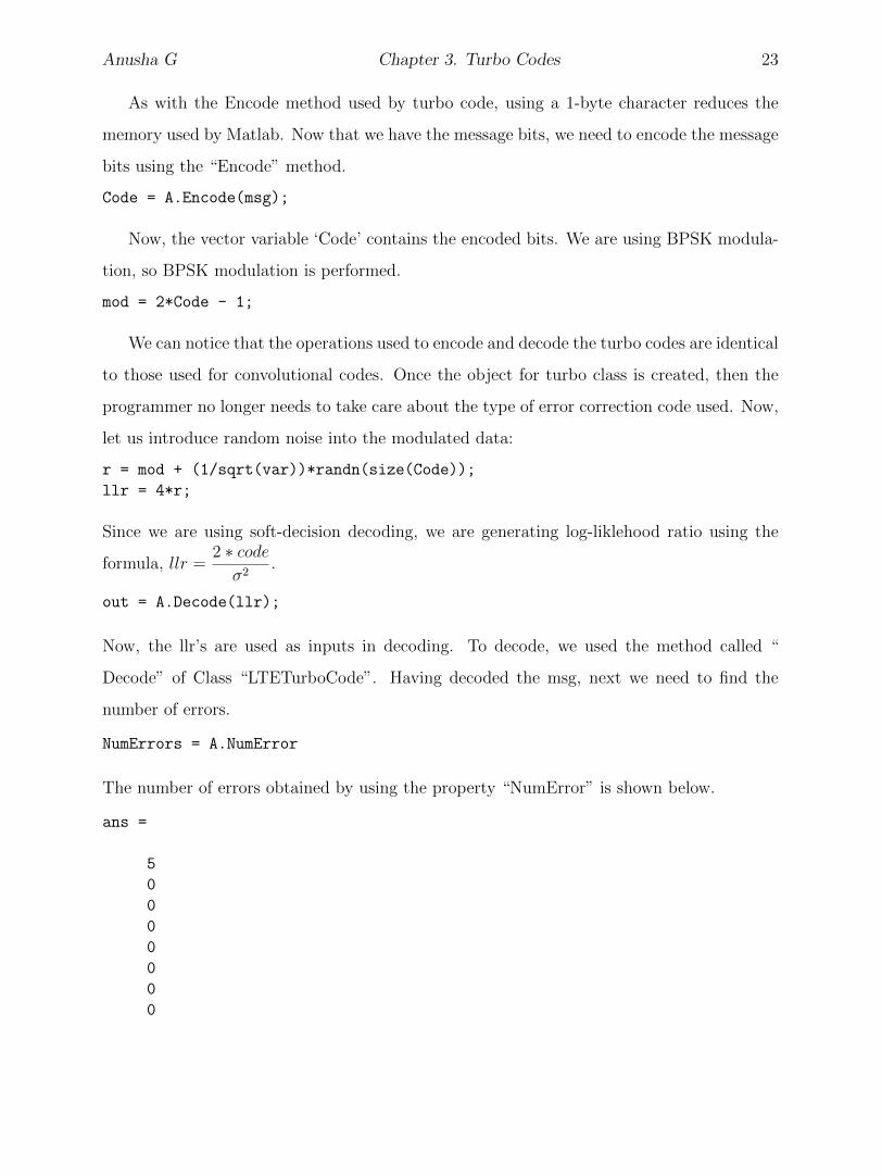
As with the Encode method used by turbo code, using a 1-byte character reduces the

memory used by Matlab. Now that we have the message bits, we need to encode the message

bits using the “Encode” method.

Code = A.Encode(msg);

Now, the vector variable ‘Code’ contains the encoded bits. We are using BPSK modula-

tion, so BPSK modulation is performed.

mod = 2*Code - 1;

We can notice that the operations used to encode and decode the turbo codes are identical

to those used for convolutional codes. Once the object for turbo class is created, then the

programmer no longer needs to take care about the type of error correction code used. Now,

let us introduce random noise into the modulated data:

r = mod + (1/sqrt(var))*randn(size(Code));

llr = 4*r;

Since we are using soft-decision decoding, we are generating log-liklehood ratio using the

formula, llr =2 ∗ codeσ2

.

out = A.Decode(llr);

Now, the llr’s are used as inputs in decoding. To decode, we used the method called “

Decode” of Class “LTETurboCode”. Having decoded the msg, next we need to find the

number of errors.

NumErrors = A.NumError

The number of errors obtained by using the property “NumError” is shown below.

ans =

5

0

0

0

0

0

0

0

24

Chapter 4

Results

Error Rate Test Console (ERTC) is a class used for running simulations provided by

Matlab’s communications toolbox. This chapter begins with a discussion of the ERTC and

later a brief working idea of ERTC is presented. Finally, the chapter concludes with the

simulation results.

4.1 Error Rate Test Console

The ERTC (Error Rate Test Console) is a class capable of running simulations for com-

munications systems to measure error rate performance. ERTC is a component of commu-

nications toolbox for running simulations.

ERTC has two main steps: creating a system and attaching the system to the test console.

A system is attached to the ERTC to run simulations and to obtain the error rate data. The

ERTC is compatible with communications systems created with a pre-defined class called

“testconsole.SystemBasicAPI class”. Some specific information has to be registered to the

ERTC in order to define the system’s test inputs, test parameters, and test probes. Once

the system is created, it has to be attached to the ERTC to run simulations.

Creating a System:

The following steps are involved in creating a system.

• Class Definition: A system class is defined by extending the properties and methods

of super class testconsole.SystemBasicAPI.

Anusha G Chapter 4. Simulation Results 25

• Registration Method: A registration method is defined, which includes test parameters,

test probes and test inputs. The methods registerTestInput, registerTestParameter,

registerTestProbe are used to register these items.

Test parameters are the system parameters for which the ERTC obtains simulation

results. We specify the sweep range of these parameters using the ERTC and obtain

simulation results for different system conditions. The system under test, registers a

system parameter to the ERTC, creating a test parameter.

The method “registerTestParameter” is used to register a test parameter to the ERTC.

The syntax is given as registerTestParamter(sys,name,default,valid range), where “sys”

represents the handle to the user-defined system object, “name” represents the param-

eter name that the system registers to the ERTC. In this problem report, “EbNo” is

used as the test parameter, “default” specifies the default value of the test parameter,

and “validRange” specifies a range of input values for the test parameter.

Test probes log the simulation data that the ERTC uses for computing test metrics

such as: number of errors, number of transmissions, and error rate. We register a test

probe to the ERTC using the method “registerTestProbe(sys,name)”, where “‘sys”

represents the handle to the user-defined system object, “name” represents the name

of the test probe.

• Run Method: The communication system for which we want to simulate results is

defined in run. Setup and Reset methods can also be defined before run method but

they are optional.

Attaching a System and Running Simulations:

The following steps are involved in attaching a system, running simulations, and gener-

ating plots.

• Create a test console by defining an object for class “commtest.ErrorRate”.

testConsole = commtest.ErrorRate;

• Now, attach the system to the ERTC to run simulations and obtain error rate data.


attachSystem(testConsole, mySystem);

“mySystem” is the LTESystem in this problem report. LTESystem includes the en-

coding and decoding of turbo codes used in LTE.

• The ERTC controls the simulation stop criterion using the “SimulationLimitOption”

property.

testConsole.SimulationLimitOption =’Number of transmissions’;

testConsole.MaxNumTransmissions = 100/1e-5;

This property stops the simulation for each parameter point when the ERTC completes

the number of transmissions specified in MaxNumTransmissions.

• The “run” method of the ERTC is used to run the simulations.

run(testConsole);

• The “getResults” method of the ERTC is used to obtain the test results.

Results = getResults(testConsole);

• Results obtained from the above method contains the information of data and is used

to plot the data. This is done using semilogy funtion.

semilogy(Results);

4.2 Performance Curves

This section gives the performance of the LTE turbo codes. Simulations were run to

determine the performance of the turbo codes using BPSK modulation in AWGN channel.

Plots show the variation of BER (Bit Error Rate) against SNR values. BER is calculated

by taking the difference between the transmitted bits and received bits (i.e., the number of

errors) divided by total number of transmitted bits.

Fig. 4.1 shows the performance of LTE turbo code with encoder input datalength of

6144 bits, modulation is BPSK and channel is AWGN. The plot shows that the performance


Figure 4.1: Performance of the datalength 6144 LTE turbo code for different decoder itera-tions. BPSK modulation and AWGN channel is considered.

improves with the increase in decoder iterations. For smaller datalengths fewer iterations are

required, but the performance improves for higher datalengths as the number of iterations

increases.

Fig. 4.2 shows the performance of LTE turbo code for different data lengths. The

performance improves as the data length increases. In the plot, we can observe that the

BER of datalength 6144 is much better than the BER of datalength 40, this is due to an

increase in the interleaver gain.


Figure 4.2: Bit Error performance of LTE Turbo system for different datalengths.


Fig. 4.3 shows the performance of LTE turbo code for linear-log-MAP and log-MAP de-

coding algorithms. From the plot it is clear that the linear-log-MAP performs approximately

0.4dB better than the log-MAP algorithm.

Figure 4.3: Plot showing the performance of the datalength 6144 LTE turbo code for differentdecoder types.

30

Chapter 5

Conclusion

This problem report presented an implementation of a specific turbo code, namely

the turbo code used by the LTE standard. Turbo codes have features like parallel code

concatenation, non-uniform interleaving and an iterative decoding algorithm. Due to these

features they can perform close to the Shannon limit. The behavior of turbo codes at low

SNR was observed for various data lengths and different decoder algorithms.

A major contribution of this report is the integration of the LTE turbo code implemen-

tation into CML2, an object-oriented version of the Coded Modulation Library. Because of

the object-oriented nature of CML2, new types of channel codes can be added with only

limited modifications to the existing code. CML2 has already implemented various channel

codes, so we can easily inherit the methods and properties of existing channel codes which

are required for our implementation using object-oriented programming.

Error Rate Test Console (ERTC) is easy to understand and implement. ERTC supports

simulation of any kind of communication system, and allows a variety of simulation parame-

ters to be adjusted. However, it has a few disadvantages like difficulty in adding new features,

and the object of the class must be created multiple times which is not desired. Otherwise,

ERTC is the most efficient and time saving component of communications toolbox. Bit error

performance plots for turbo codes are obtained for various parameters and we are able to

observe the behavior of turbo codes.

Based on the work presented in this problem report, a few ideas are suggested for future

work. ERTC has drawbacks like difficulty in adding new features to a user-defined com-

Anusha G Chapter 5. Conclusion 31

munications system to obtain error rate analysis. To overcome this, a fully object-oriented

simulation environment where the users can make changes according to their requirements

can be developed, which will be helpful for running simulations independent of type of chan-

nel code used. Furthermore, support for LTE rate matching pattern can be added which

allows the LTE turbo code to achieve a wide range of code rates.

32

References

[1] N. Chandran and M.C. Valenti, “Three generations of wireless cellular systems,” IEEEPotentials, vol. 20, no. 1, pp. 32–35, Feb./March 2001.

[2] G.L. Stuber, Principles of Mobile Communication, Kluwer Academic Publishers, 1996.

[3] E. Eyre, “Verizon announces 4g network for state,” Charleston Gazette, Oct. 27, 2010.

[4] Andrea Goldsmith, Wireless Communications, Cambridge University Press, 2005.

[5] C. Berrou, A. Glavieux, and P. Thitimasjshima, “Near Shannon limit error-correctingcoding and decoding: Turbo-codes(1),” in Proc. IEEE Int. Conf. on Commun. (ICC),Geneva, Switzerland, May 1993, pp. 1064–1070.

[6] Simon Haykin, Jose C.Prancipe, Terrence J.Sejnolwski, and John McWhirter, NewDirections in Statistical signal processing, The MIT Press, third edition, 2006.

[7] Rodger E. Ziermer and Roger L. Peterson, Introduction to Digital Communications,Prentice Hall, second edition, 2001.

[8] T. S. Rappaport, Wireless Communications: Principles and Practice, Prentice HallPTR, Upper Saddle River, NJ, second edition, 2002.

[9] Shu Lin and Jr. Daniel J. Costello, Error Control Coding, Prentice Hall, second edition,2004.

[10] Matthew C. Valenti, “Coded modulation library,” http://www.iterativesolutions.com.

[11] J. Proakis, Digital Communications, McGraw-Hill, Inc., New York, NY, fourth edition,2001.

[12] B. P. Lathi, Modern Digital and Analog Communication Systems, Oxford UniversityPress, third edition, 1998.

[13] M.C. Valenti, Iterative detection and decoding for wireless communications, Ph.D.thesis, Virginia Polytechnic Institute and State University, Blacksburg, VA, 1999.

[14] C. Heegard and S.B. Wicker, Turbo Coding, Kluwer Academic Publishers, Dordrecht,the Netherlands, 1999.

REFERENCES 33

[15] Third Generation Partnership Project, “Evolved universal terrestrial radio access (E-UTRA): Multiplexing and channel coding,” 3GPP TS 36.212 version 9.2.0, May 31,2007.

[16] M. C. Valenti and J.Sun, “Turbo codes,” in Handbook of RF and Wireless Technologies,F.Dowla Editor, Ed., chapter 12. Newnes Press, 2004.

[17] P. Hoeher, “New iterative (‘turbo’) decoding algorithms,” Int. Symp. on Turbo Codesand Related Topics, pp. 63–70, Sept. 1997.

[18] A. Anastasopoulos K. Chugg and X. Chen, Iterative Detection:Adaptivity, ComplexityReduction and Applications, Kluwer Academic Publishers, Dordrecht, the Netherlands,2001.

[19] Matthew C. Valenti, “Turbo codes and iterative processing,” IEEE New ZealandWireless Communication symp.,(Auckland, New Zealand), Nov. 1998.

[20] P. Robertson, P. Hoeher, and E. Villebrun, “Optimal and sub-optimal maximum aposteriori algorithms suitable for turbo decoding,” European Trans. on Telecommun.,vol. 8, no. 2, pp. 119–125, Mar./Apr. 1997.

Documents

Object-Oriented Implementation of LTE Turbo Codes - …wvuscholar.wvu.edu/reports/Gangadi_Anusha.pdf · Abstract Object-Oriented Implementation of LTE Turbo Codes by Anusha Gangadi