Object Manipulation using a Multirobot Cluster with Force

Santa Clara UniversityScholar Commons

Mechanical Engineering Master's Theses Engineering Master's Theses

6-5-2017

Object Manipulation using a Multirobot Clusterwith Force SensingMatthew H. ChinSanta Clara University, [email protected]

Follow this and additional works at: http://scholarcommons.scu.edu/mech_mstr

Part of the Mechanical Engineering Commons

This Thesis is brought to you for free and open access by the Engineering Master's Theses at Scholar Commons. It has been accepted for inclusion inMechanical Engineering Master's Theses by an authorized administrator of Scholar Commons. For more information, please [email protected].

Recommended CitationChin, Matthew H., "Object Manipulation using a Multirobot Cluster with Force Sensing" (2017). Mechanical Engineering Master'sTheses. 11.http://scholarcommons.scu.edu/mech_mstr/11

http://scholarcommons.scu.edu?utm_source=scholarcommons.scu.edu%2Fmech_mstr%2F11&utm_medium=PDF&utm_campaign=PDFCoverPages

http://scholarcommons.scu.edu/mech_mstr?utm_source=scholarcommons.scu.edu%2Fmech_mstr%2F11&utm_medium=PDF&utm_campaign=PDFCoverPages

http://scholarcommons.scu.edu/eng_master_theses?utm_source=scholarcommons.scu.edu%2Fmech_mstr%2F11&utm_medium=PDF&utm_campaign=PDFCoverPages

http://scholarcommons.scu.edu/mech_mstr?utm_source=scholarcommons.scu.edu%2Fmech_mstr%2F11&utm_medium=PDF&utm_campaign=PDFCoverPages

http://network.bepress.com/hgg/discipline/293?utm_source=scholarcommons.scu.edu%2Fmech_mstr%2F11&utm_medium=PDF&utm_campaign=PDFCoverPages

http://scholarcommons.scu.edu/mech_mstr/11?utm_source=scholarcommons.scu.edu%2Fmech_mstr%2F11&utm_medium=PDF&utm_campaign=PDFCoverPages

mailto:[email protected]

Object Manipulation using a Multirobot Cluster with Force Sensing

by

Matthew H. Chin

GRADUATE MASTERS THESIS

Submitted in partial fulfillment of the requirementsfor the degree of

Master of Science in Mechanical EngineeringSchool of EngineeringSanta Clara University

Santa Clara, California

June 5, 2017

Object Manipulation using a Multirobot Cluster with Force Sensing

Matthew H. Chin

Department of Mechanical EngineeringSanta Clara University

2017

ABSTRACT

This research explored object manipulation using multiple robots by developing a control

system utilizing force sensing. Multirobot solutions provide advantages of redundancy,

greater coverage, fault-tolerance, distributed sensing and actuation, and reconfigurability.

In object manipulation, a variety of solutions have been explored with different robot

types and numbers, control strategies, sensors, etc. This research involved the integration

of force sensing with a centralized position control method of two robots (cluster control)

and building it into an object level controller. This controller commands the robots to

push the object based on the measured interaction forces between them while maintaining

proper formation with respect to each other and the object.

To test this controller, force sensor plates were attached to the front of the Pioneer 3-AT

robots. The object is a long, thin, rectangular prism made of cardboard, filled with paper

for weight. An Ultra Wideband system was used to track the positions and headings of

the robots and object. Force sensing was integrated into the position cluster controller by

decoupling robot commands, derived from position and force control loops.

The result was a successful pair of experiments demonstrating controlled transportation

of the object, validating the control architecture. The robots pushed the object to follow

linear and circular trajectories. This research is an initial step toward a hybrid

force/position control architecture with cluster control for object transportation by a

multirobot system.

Keywords: cluster space control, force sensing, multirobot, force manipulation, object transportation

iii

Acknowledgements

I would foremost like to thank my advisor, Dr. Christopher Kitts. From the beginning of

my time here at Santa Clara University, he welcomed me to the program and the lab with

the same joy he has today. I am thankful for his tutelage, continued encouragement,

patience, and positive guidance.

I would also like to thank everyone in the Santa Clara University Robotics Systems

Laboratory. After working alongside you all and seeing all the creative projects produced

from the lab, I have been inspired to work harder. I would like to thank Mike Rasay for

his nuggets of wisdom. I will especially remember your emphasis of the 7 P's (Proper,

Prior Planning Prevents Piss, Poor Performance!). I would like to thank Thomas

Adamek and Ketan Rasal, the first people I worked alongside in the lab, for teaching me

and including me in their field research. I would also like to thank the quadrotor research

group of Jasmine Cashbaugh, Anne Mahacek, Christian Zempel, and Alicia Sherban for

sharing the Ultra Wideband testing area. I would like to thank Michael Valhos for his

software expertise. I also greatly thank Jackson Arcade and Michael Neumann. We

developed the testbed together and our collective work was instrumental in the

completion of this research. I am glad I had them to brainstorm with when

troubleshooting unexpected results.

Finally, I would like to thank my family and friends for their encouragement and support.

Specifically to my parents, I thank you for your limitless support in all its forms. I thank

you for your wisdom, given not only when I asked for it, but also when I needed to hear

it. I would not be who I am today without you.

iv

Table of Contents

Abstract...............................................................................................................................iii

Acknowledgments..............................................................................................................iv

Table of Contents.................................................................................................................v

List of Figures....................................................................................................................vii

List of Abbreviations............................................................................................................x

List of Equations.................................................................................................................xi

Chapter 1: Introduction........................................................................................................1

1.1 Prior Work in Multirobot System Object Manipulation..........................................1

1.2 Project Statement.....................................................................................................6

1.3 Reader's Guide.........................................................................................................7

Chapter 2: Control Methodology.........................................................................................8

2.1 Introduction to Cluster Space Control.....................................................................8

2.2 Global and Cluster Space Variables and Equations for a two-robot cluster............9

2.3 Cluster Control System with Force Sensing..........................................................15

Chapter 3: Experimental Testbed.......................................................................................20

3.1 System Overview...................................................................................................20

3.2 Object.....................................................................................................................20

3.3 Robots....................................................................................................................22

3.4 Position Sensor System..........................................................................................24

3.5 Data Flow...............................................................................................................25

Chapter 4: Experiment.......................................................................................................27

4.1 Linear Path.............................................................................................................27

v

4.2 Circular Trajectory Path.........................................................................................30

4.3 Summary................................................................................................................32

Chapter 5: Conclusion........................................................................................................33

5.1 Future Work...........................................................................................................33

References..........................................................................................................................35

Appendix..........................................................................................................................A-1

A.1 Arduino code for collecting and filtering force data...........................................A-1

A.2 Simulink Model of the Control System..............................................................A-5

A.3 Simulink Block Code........................................................................................A-20

vi

List of Figures

Figure 1.1: Four types of object manipulation.....................................................................2

Figure 1.2: Pusher-Watcher experimental setup..................................................................3

Figure 1.3: NASA CAMPOUT multirobot transport formation..........................................5

Figure 1.4: USNA experimental scale model......................................................................6

Figure 2.1: Reference Frames............................................................................................10

Figure 2.2: Robot Coordinates...........................................................................................11

Figure 2.3: Cluster Control Architecture...........................................................................15

Figure 2.4: Adapted Force Control Strategy......................................................................16

Figure 2.5: Cluster Control Architecture with Force Sensing............................................17

Figure 2.6: Line Controller................................................................................................18

Figure 3.1: Testbed Photo..................................................................................................20

Figure 3.2: Testbed Overhead View...................................................................................21

Figure 3.3: Robots and Object in Test Area.......................................................................22

Figure 3.4: Communications Equipment...........................................................................23

Figure 3.5: Force Plate and Mount....................................................................................23

Figure 3.6: Force Sensor Processing and Communication Equipment..............................24

Figure 3.7: Position Sensor System Components..............................................................25

Figure 3.8: Data Communications Diagram......................................................................26

Figure 4.1: Experiment 1 Illustration.................................................................................28

Figure 4.2: Experiment 1 Results: Overhead View............................................................28

Figure 4.3: Experiment 1 Crosstrack error.........................................................................29

Figure 4.4: Experiment 1 Force Sensor Plate Responses..................................................29

vii

Figure 4.5: Experiment 2 Results: Overhead View............................................................30

Figure 4.6: Experiment 2 Crosstrack Error from Circular Path.........................................31

Figure 4.7: Experiment 2 Force Sensor Plate Responses..................................................32

Figure A.1: Straight Line Path Following Control System Simulink Model..................A-6

Figure A.2: Control System Part 1(top-left section)........................................................A-7

Figure A.3: Control System Part 2 (top-right section).....................................................A-8

Figure A.4: Control System Part 3 (bottom-left section).................................................A-9

Figure A.5: Control System Part 4 (bottom-right section)............................................A-10

Figure A.6: Control System Part 1: 2-Robot Cluster Inverse Velocity Kinematics Block....

.......................................................................................................................................A-11

Figure A.7: Control System Part 4: Cluster fwd Position Kinematics Block...............A-11

Figure A.8: Control System Part 4: Cluster Forward Velocity Kinematics Block.........A-11

Figure A.9: Control System Part 3: Heading Ctrl Block...............................................A-11

Figure A.10: Control System Part 4: Force Controller Block.......................................A-12

Figure A.11: Force Controller: PI Control Block..........................................................A-12

Figure A.12: Control System Part 3: Box Tag Data Block............................................A-12

Figure A.13: Control System Part 2: Plant Pioneer Block.............................................A-13

Figure A.14: Plant Pioneer Block: Rover Local to Global Frame Transform Block.....A-14

Figure A.15: Plant Pioneer Block: Cluster to Robot Block...........................................A-14

Figure A.16: Plant Pioneer Block: UWB to Cluster Block...........................................A-14

Figure A.17: Box Tag Data Block: DAQ Block............................................................A-14

Figure A.18: Plant Pioneer Block: Heading Ctrl Block.................................................A-15

Figure A.19: Plant Pioneer Block: Pioneer Tag Data Block..........................................A-16

viii

Figure A.20: Cluster to UWB Block..............................................................................A-16

Figure A.21: Pioneer Tag Data Block: Tag Filter Block................................................A-16

Figure A.22: Tag Filter Block: Moving Average Block.................................................A-16

Figure A.23: Circle Path Following Control System Simulink Model..........................A-17

Figure A.24: Circle Following Control System Part 3 (bottom-left section)................A-18

Figure A.25: Control System Part 3: meta ctrl block.....................................................A-19

Figure A.26: Control System Part 3: Line Controller....................................................A-19

ix

List of Abbreviations

• CAMPOUT – Control Architecture for Multirobot Planetary Outposts

• DOF – degrees-of-freedom

• JPL – Jet Propulsion Laboratory

• NASA – National Aeronautics and Space Administration

• PRL – Planetary Robotics Laboratory

• RFID – Radio Frequency Identification

• RMS – Root Mean Square

• RSL – Robotic Systems Laboratory

• SCU – Santa Clara University

• SRR – Sample-Return Rover

• SWATH – Small Waterplane Area Twin Hull

• USNA – United States Naval Academy

• UWB – Ultra Wideband

x

List of Equations

Forward Kinematic Equations

Eq. 2.1....................................................................................................................11

Eq. 2.2....................................................................................................................11

Eq. 2.3....................................................................................................................11

Eq. 2.4....................................................................................................................12

Eq. 2.5....................................................................................................................12

Eq. 2.6....................................................................................................................12

Inverse Kinematic Equations

Eq. 2.7....................................................................................................................12

Eq. 2.8....................................................................................................................12

Eq. 2.9....................................................................................................................12

Eq. 2.10..................................................................................................................12

Eq. 2.11..................................................................................................................12

Eq. 2.12..................................................................................................................12

Partial Derivatives of the Forward Kinematic Equations

Eq. 2.13..................................................................................................................13

Eq. 2.14..................................................................................................................13

Eq. 2.15..................................................................................................................13

Eq. 2.16..................................................................................................................13

Eq. 2.17..................................................................................................................13

Eq. 2.18..................................................................................................................13

xi

Partial Derivatives of the Inverse Kinematic Equations

Eq. 2.19..................................................................................................................13

Eq. 2.20..................................................................................................................13

Eq. 2.21..................................................................................................................13

Eq. 2.22..................................................................................................................13

Eq. 2.23..................................................................................................................13

Eq. 2.24..................................................................................................................13

Eq. 2.25..................................................................................................................14

Eq. 2.26..................................................................................................................14

Forward and Inverse Jacobian Matrices

Eq. 2.27..................................................................................................................14

Eq. 2.28..................................................................................................................14

Line Controller Equations

Eq. 2.29..................................................................................................................18

Eq. 2.30..................................................................................................................18

Eq. 2.31..................................................................................................................19

xii

1 Introduction

Robot applications are increasingly widespread, automating steps of industrial

production, aiding in medical procedures, serving as research tools, performing

household chores, and more. They are designed to emulate human sensing, actuation,

and other functions with advantages like greater accuracy, precision, repeatability,

dexterity, strength and speed, allowing them to perform certain tasks extremely well.

Robotic solutions have led to many improvements in industrial, military, space

exploration, agriculture, and medical fields to name a few.

While optimizing single robotic solutions for emulating a human's abilities offer great

advantages, multirobot solutions can offer many more. As some tasks require more than

one person to perform, a multirobot system can be developed to perform coordinated

tasks. Multirobot systems offer advantages such as redundancy, greater coverage, fault-

tolerance, distributed sensing and actuation, and reconfigurability [6]. Examples of

applications are: escorting, increasing signal coverage, transporting large objects,

tracking objects, performing distributed environmental sensing, and other cooperative

tasks.

1.1 Prior Work in Multirobot System Object Manipulation

Objects can be manipulated in different ways. Some robots lift and transport the object,

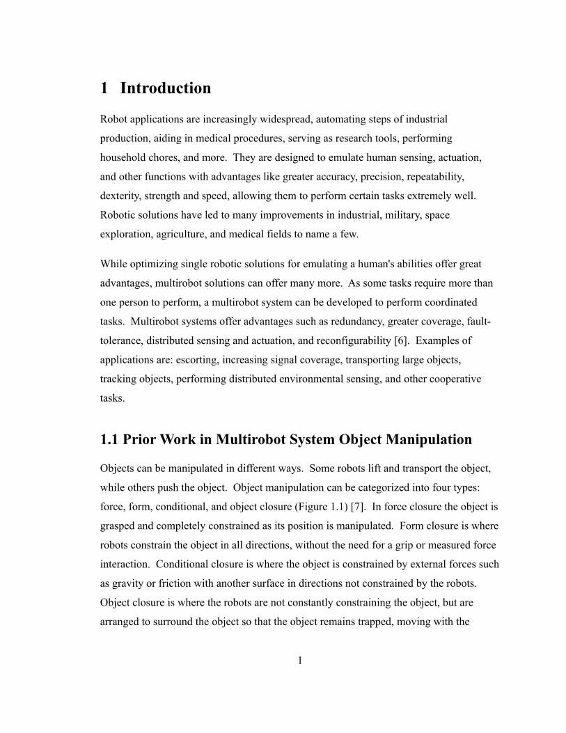
while others push the object. Object manipulation can be categorized into four types:

force, form, conditional, and object closure (Figure 1.1) [7]. In force closure the object is

grasped and completely constrained as its position is manipulated. Form closure is where

robots constrain the object in all directions, without the need for a grip or measured force

interaction. Conditional closure is where the object is constrained by external forces such

as gravity or friction with another surface in directions not constrained by the robots.

Object closure is where the robots are not constantly constraining the object, but are

arranged to surround the object so that the object remains trapped, moving with the

1

robots [24, 27]. Using different resources and approaches, different methods were

developed. Some variations of those four types that have been explored are pusher-

watcher, pusher-puller, pusher-steerer, leader-follower (master-slave), and swarm

manipulation strategies.

The pusher-puller and pusher-steerer strategies are examples of form closure. The

pusher-puller method, from a group at Seoul National University [7], involves two robots

attached to an object at its back and front sides with hook and loop fasteners and which

respectively push and pull the object simultaneously without any force feedback. The

pusher-steerer strategy is attached similarly to an object but the front robot only steers as

the rear robot pushes the object, like a rear wheel drive car [4]. The robots can switch

steering and pushing roles for easier movement of the object.

2

Figure 1.1: Four types of object manipulation. Force closure (a), form closure (b), conditional closure (c), object closure (d)

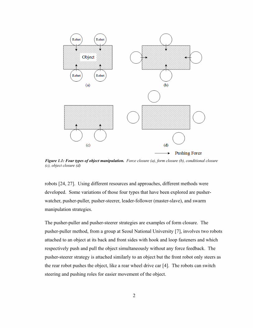
An example of conditional closure comes from [25]. Without explicit knowledge of the

object dynamics and characteristics, a pair of decentralized, six-legged robots,

programmed with a turn-taking control system, pushed on the same side of an elongated

box toward a lighted goal. Some of the same researchers also developed a pusher-

watcher strategy. This strategy mimicked how humans can work together to push large

objects with external direction from another person with a clear point of view of the

object and goal. Two non-holonomic, wheeled robots pushed a long rectangular box

from the same side. A robot on the other side of the rectangular box, at a distance,

tracked the box's angle and position with respect to the goal location (Figure 1.2). That

information was processed through their task-allocation framework, MURDOCH, which

sent updated commands to the pusher robots. The box's dynamics are not being used in

the control system [10]. Another group of researchers used a similar strategy to push an

object in water using autonomous robotic fish [11, 36].

An example of object closure is a decentralized caging strategy. Three robots with 7DOF

manipulator arms use their motorized bases and end effectors to cage an object and move

3

Figure 1.2: Pusher-Watcher experimental setup. Goal, rectangular box, a watcher robot and two pusher robots. The pusher robots push the robot toward the goal with direction from the watcher robot. [1]

it to a goal [35]. To improve the object closure strategy, a potential field approach was

implemented to improve how the robots surround and transport the object [8, 29]. The

robots have knowledge of their neighboring robots' positions to properly trap the object

while avoiding collisions. The cluster space approach also was adapted to cage and

transport an object with object closure [16].

Another method of object manipulation is to use swarms of robots. Taking cues from

nature like ants, swarm manipulation usually consists of a large number of small robots

working independently toward a similar goal with little to no information of their fellow

robots. There are many unique approaches to swarm control. One research group

simulated a task allocation strategy that was improved using an ant colony algorithm

pheromone updating rule [20]. Another group introduced a mediator position to better

organize swarms and reduce flocking and fragmentation [14]. A different group

developed a swarm of 10 robots with light and push sensors. Based on light and touch

sensor input, the robots would independently perform certain subtasks to achieve the

overall goal of moving a large object to a goal location [19].

These strategies are effective in certain conditions but without force or torque sensing,

there is a risk of damaging the object or the robots if unsafe magnitudes of force were to

occur. The following are similar strategies of closure, but include force control or

sensing to move objects. There are examples of force closure with grasping manipulators

such as stationary arms with end effectors using active force control and constrained

motion [15], grasp control from humanoid robots [30], and grippers on mobile platforms

[32, 33]. The NASA Jet Propulsion Laboratory (JPL) developed an autonomous,

multirobot system as part of a plan for constructing structures for exploration on the

moon and Mars. Two holonomic robots with four wheels, a four degree-of-freedom arm,

and a gripper with a 3-axis force-torque sensor operated autonomously with a behavior-

based, leader-follower control architecture called Control Architecture for Multirobot

Planetary OUTposts (CAMPOUT). Transportation of long beams for building structures

is one of the tasks the pair of robots is programmed for. The leader and follower robots,

named SRR and SRR2K, respectively, hold a beam near each end between their grippers.

4

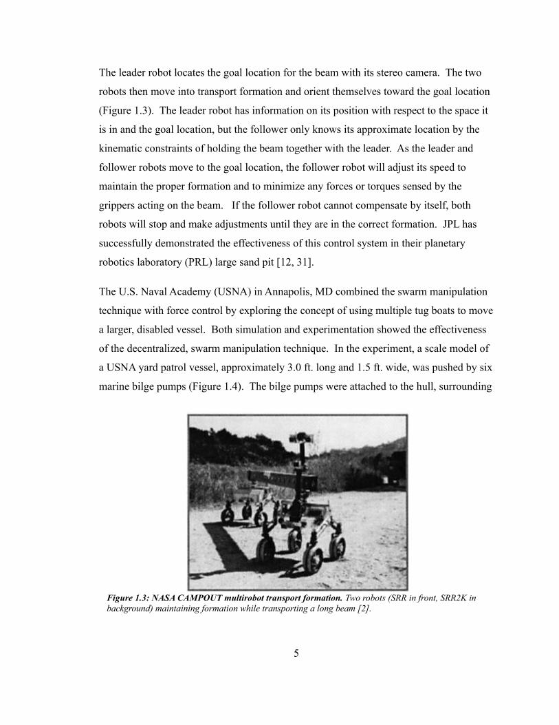
The leader robot locates the goal location for the beam with its stereo camera. The two

robots then move into transport formation and orient themselves toward the goal location

(Figure 1.3). The leader robot has information on its position with respect to the space it

is in and the goal location, but the follower only knows its approximate location by the

kinematic constraints of holding the beam together with the leader. As the leader and

follower robots move to the goal location, the follower robot will adjust its speed to

maintain the proper formation and to minimize any forces or torques sensed by the

grippers acting on the beam. If the follower robot cannot compensate by itself, both

robots will stop and make adjustments until they are in the correct formation. JPL has

successfully demonstrated the effectiveness of this control system in their planetary

robotics laboratory (PRL) large sand pit [12, 31].

The U.S. Naval Academy (USNA) in Annapolis, MD combined the swarm manipulation

technique with force control by exploring the concept of using multiple tug boats to move

a larger, disabled vessel. Both simulation and experimentation showed the effectiveness

of the decentralized, swarm manipulation technique. In the experiment, a scale model of

a USNA yard patrol vessel, approximately 3.0 ft. long and 1.5 ft. wide, was pushed by six

marine bilge pumps (Figure 1.4). The bilge pumps were attached to the hull, surrounding

5

Figure 1.3: NASA CAMPOUT multirobot transport formation. Two robots (SRR in front, SRR2K in background) maintaining formation while transporting a long beam [2].

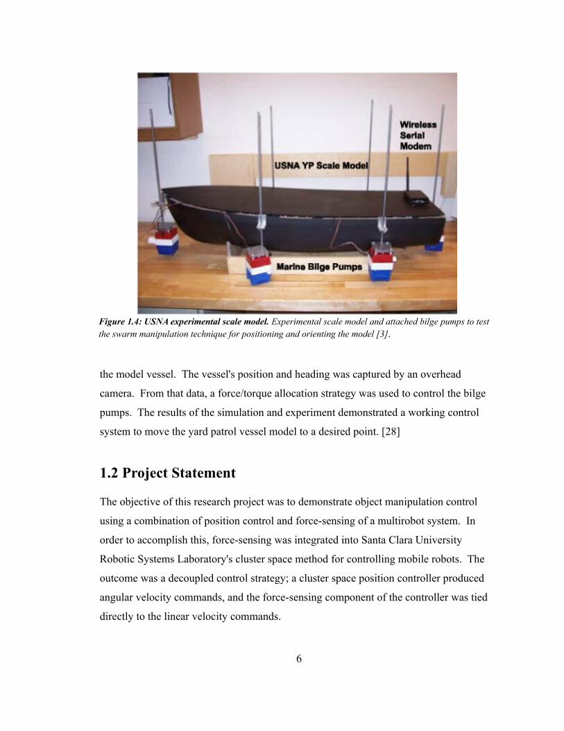
the model vessel. The vessel's position and heading was captured by an overhead

camera. From that data, a force/torque allocation strategy was used to control the bilge

pumps. The results of the simulation and experiment demonstrated a working control

system to move the yard patrol vessel model to a desired point. [28]

1.2 Project Statement

The objective of this research project was to demonstrate object manipulation control

using a combination of position control and force-sensing of a multirobot system. In

order to accomplish this, force-sensing was integrated into Santa Clara University

Robotic Systems Laboratory's cluster space method for controlling mobile robots. The

outcome was a decoupled control strategy; a cluster space position controller produced

angular velocity commands, and the force-sensing component of the controller was tied

directly to the linear velocity commands.

6

Figure 1.4: USNA experimental scale model. Experimental scale model and attached bilge pumps to test the swarm manipulation technique for positioning and orienting the model [3].

A force-sensing system, the controller and the sensor attachment to the mobile robots,

were co-developed with fellow student Jackson Arcade. The result of this research was a

successful demonstration that the cluster space control technique can be modified with

force-sensing to perform controlled manipulation of an object’s position. This is an

example of the expansive possibilities of the cluster control technique, specifically in the

object manipulation field. From this research, further exploration into multirobot

manipulation techniques with cluster space control can be developed, such as the

development of a full hybrid position-force controller.

1.3 Reader's Guide

This thesis is composed of five chapters. The first chapter contains an introduction of

multirobot strategies for object manipulation. The project statement of this thesis is also

stated here. The second chapter describes the previously developed cluster control

technique and how force-sensing was added to the control system. Derivations of the

cluster control variables are stated here. The third chapter discusses the hardware and

experimental setup. The fourth chapter discusses the experiment and the effectiveness of

the control system. The fifth chapter summarizes the thesis project, results, and lists

future work to take this research further.

7

2 Control Methodology

The cluster control method simplifies simultaneous control of multiple robots by using

pose variables to characterize the robots as parts of a single cluster. It allows the user to

focus on a group of robots completing tasks as a single entity. The task for this thesis is

to use a two-robot cluster with force-sensing to implement a controlled push on an object,

following a desired path. The control system translates desired motion for the cluster into

a desired force and torque for the cluster to apply to the object. Force sensor push plates,

mounted on the front of each robot, provide force feedback between the robots and the

object being pushed. The cluster-level force control system uses this sensor data to

achieve the desired force and torque by varying cluster velocity commands, which, in

turn, are converted into individual robot velocity commands. This chapter defines the

cluster control system, describes the relevant transformation equations and the different

reference frames, and explains how the force sensing component is added to a typical

position-based cluster control system.

2.1 Introduction to Cluster Space Control

Instead of controlling a group of robots with a set of variables assigning the positions and

orientations of each individual robot, the robots are treated as a single “virtual” entity,

called a cluster. The cluster has its own defined position, orientation, and shape variables

dictating the positions and orientation of all the robots that are a part of the cluster.

Examples of a cluster's defined position in space could be the cluster's centroid or the

position of one of the robots in the cluster. The orientation of the cluster could be

determined by defining one of its reference axes from the cluster's centroid to the position

of one of the cluster's robots. The robot arrangement is defined through cluster shape

variables. Some examples of these shape variables are the distance a robot is from the

cluster's centroid, the distance between robots in the same cluster, and the angle created

between multiple robots. Cluster variables have a kinematic relationship with the

individual robot position and orientation variables. Forward kinematic equations can

8

transform the individual robot variables to cluster variables. Inverse kinematic equations

reverse the transformation. The partial derivatives of these equations result in equations

that transform individual robot velocity commands to cluster velocity commands and

vice-versa. These equations are factored and expressed in terms of Jacobian matrices.

Defining the robots using cluster space allows planning of the formation and movements

in more abstract cluster space variables related to the task instead of planning the

trajectories of each individual robot. This method was used in other Santa Clara

University teams' research with blimps [2], quadcopters [5], and autonomous surface

vessels [17, 21, 22, 23].

2.2 Global and Cluster Space Variables and Equations for a

two-robot cluster

For the experiments performed in this thesis, two robots operated in a planar test area

approximately 13 by 19 meters in size. A global frame was defined with its origin at the

center of the workspace and with unit vectors oriented using an aerospace convention.

An Ultra Wideband (UWB) tracking system was set up in this test area to track tags

placed on each robot. Its frame was defined with the origin at the same location as the

origin of the global frame, and with unit vectors as per the manufacturer’s specification.

Two robots operated in the plane with two UWB tags each placed across the robots'

centroids. The average of the tags' positions is the origin of the robot frame for each

robot. Velocity commands are transformed into this frame to execute the desired robot

maneuvers. The frames were defined with the x-axis pointing toward the front of the

robot, the y-axis pointing to the left of the robot, and the z-axis pointing upwards from

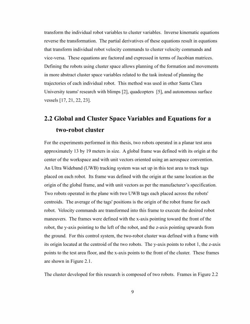
the ground. For this control system, the two-robot cluster was defined with a frame with

its origin located at the centroid of the two robots. The y-axis points to robot 1, the z-axis

points to the test area floor, and the x-axis points to the front of the cluster. These frames

are shown in Figure 2.1.

The cluster developed for this research is composed of two robots. Frames in Figure 2.2

9

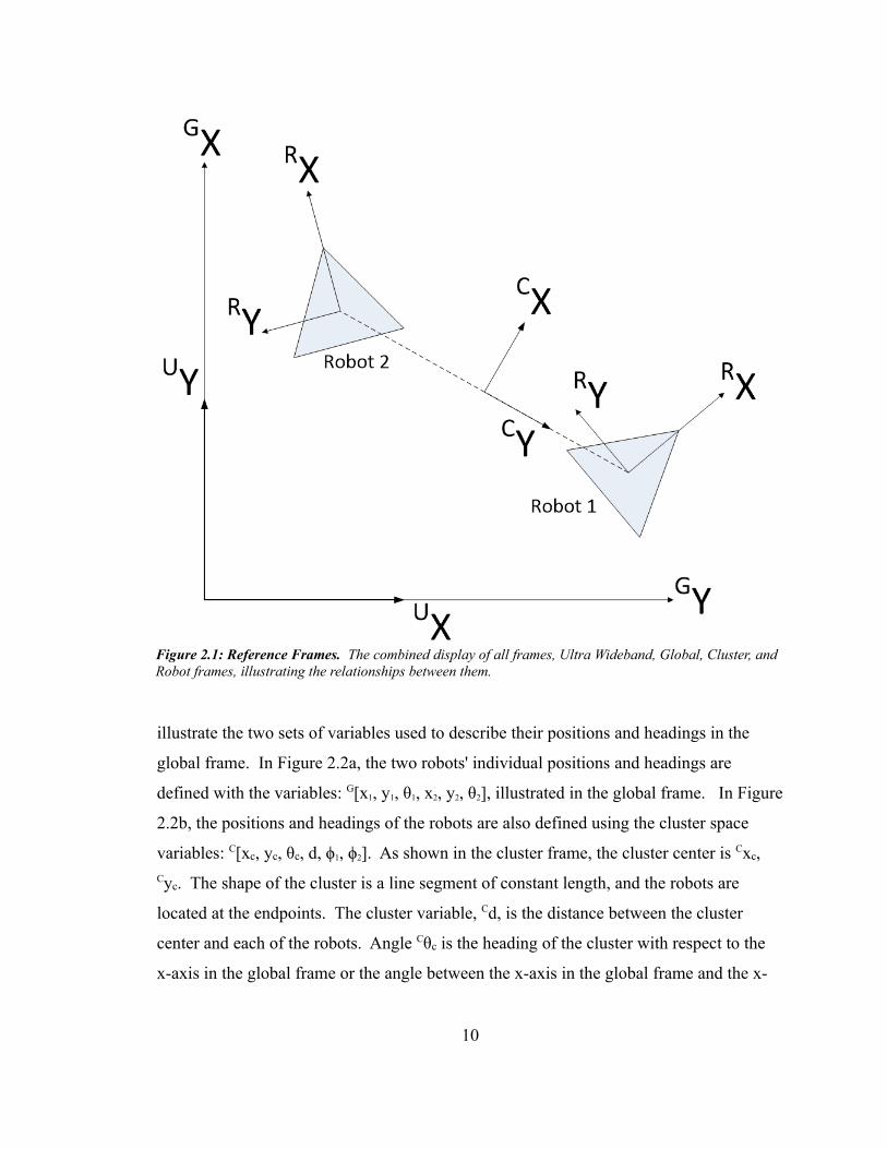
illustrate the two sets of variables used to describe their positions and headings in the

global frame. In Figure 2.2a, the two robots' individual positions and headings are

defined with the variables: G[x1, y1, θ1, x2, y2, θ2], illustrated in the global frame. In Figure

2.2b, the positions and headings of the robots are also defined using the cluster space

variables: C[xc, yc, θc, d, ϕ1, ϕ2]. As shown in the cluster frame, the cluster center is Cxc, Cyc. The shape of the cluster is a line segment of constant length, and the robots are

located at the endpoints. The cluster variable, Cd, is the distance between the cluster

center and each of the robots. Angle Cθc is the heading of the cluster with respect to the

x-axis in the global frame or the angle between the x-axis in the global frame and the x-

10

Figure 2.1: Reference Frames. The combined display of all frames, Ultra Wideband, Global, Cluster, andRobot frames, illustrating the relationships between them.

axis in the cluster frame. Angles Cϕ1 and Cϕ2 are the two robots' individual headings with

respect to the x-axis in the cluster frame. These six cluster variables fully describe the

robots' positions and headings as part of a cluster.

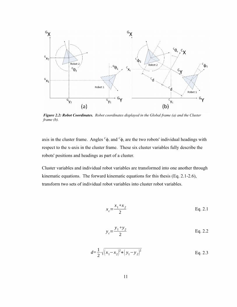
Cluster variables and individual robot variables are transformed into one another through

kinematic equations. The forward kinematic equations for this thesis (Eq. 2.1-2.6),

transform two sets of individual robot variables into cluster robot variables.

xc=x1+x 2

2Eq. 2.1

yc=y1+y2

2Eq. 2.2

d=12⋅√(x1−x2)2+( y1−y 2)2 Eq. 2.3

11

Figure 2.2: Robot Coordinates. Robot coordinates displayed in the Global frame (a) and the Cluster frame (b).

θc =atan( x1−x2y1− y2) Eq. 2.4

ϕ1=θ1−atan( x1−x2y1−y2 ) Eq. 2.5

ϕ2=θ2−atan( x1−x2y1−y2) Eq. 2.6

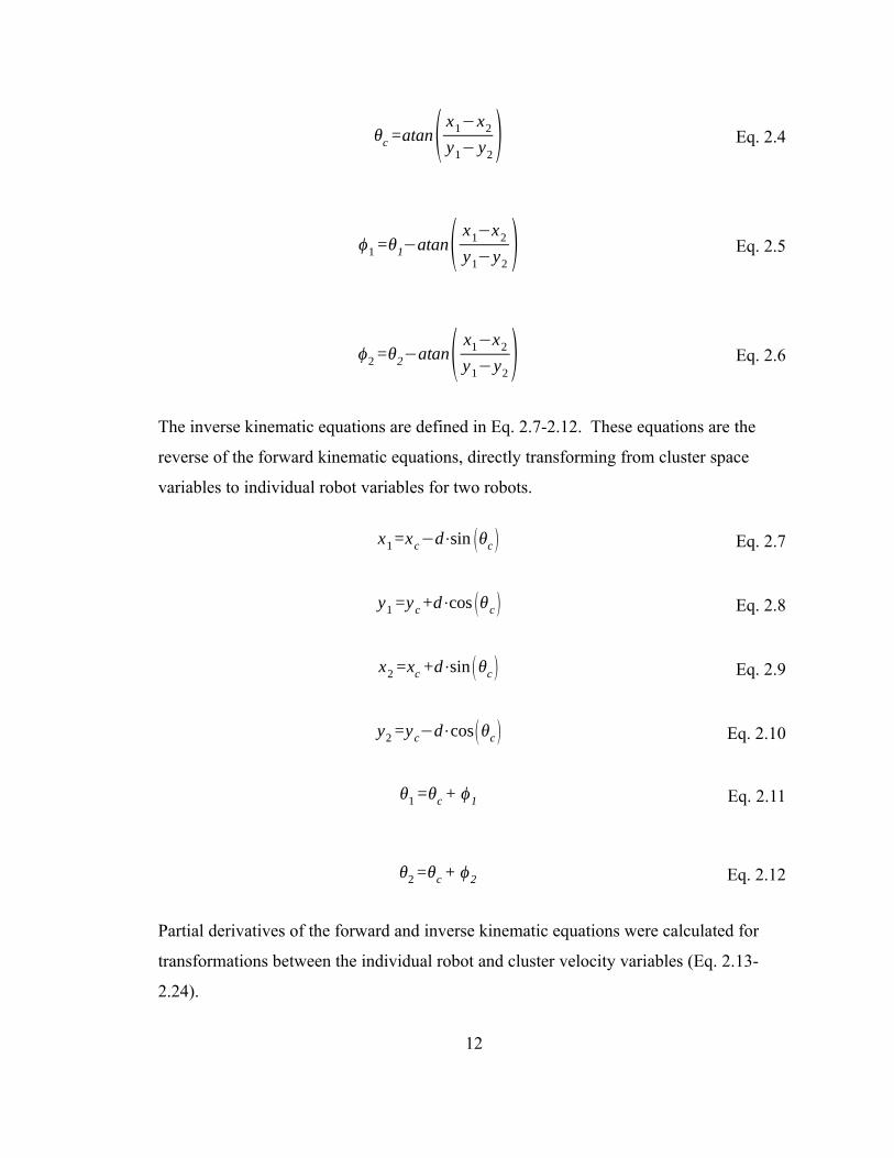
The inverse kinematic equations are defined in Eq. 2.7-2.12. These equations are the

reverse of the forward kinematic equations, directly transforming from cluster space

variables to individual robot variables for two robots.

x1=xc−d⋅sin (θc) Eq. 2.7

y1=yc+d⋅cos (θc) Eq. 2.8

x2=xc +d⋅sin(θc) Eq. 2.9

y2=yc−d⋅cos(θc) Eq. 2.10

θ1=θc + ϕ1 Eq. 2.11

θ2=θc + ϕ2 Eq. 2.12

Partial derivatives of the forward and inverse kinematic equations were calculated for

transformations between the individual robot and cluster velocity variables (Eq. 2.13-

2.24).

12

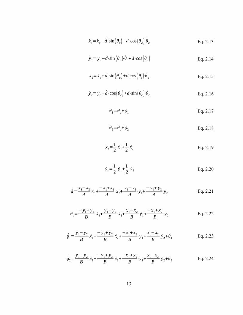
x1= xc−d⋅sin (θc)−d⋅cos (θc)⋅θc Eq. 2.13

y1= yc−d⋅sin (θc )⋅θc+ d⋅cos (θc) Eq. 2.14

x2= xc+ d⋅sin(θc)+d⋅cos (θc)⋅θc Eq. 2.15

y2= yc−d⋅cos(θc)+d⋅sin (θc)⋅θc Eq. 2.16

θ1=θc+ ϕ1 Eq. 2.17

θ2=θc+ ϕ2 Eq. 2.18

xc=12⋅x1+

12⋅x2 Eq. 2.19

yc=12⋅y1+

12⋅y2 Eq. 2.20

d=x1−x2

A⋅x1+

−x1+x2A

⋅x2+y1−y2

A⋅y1+

− y1+ y2A

⋅y2 Eq. 2.21

θc=− y1+ y2

B⋅x1+

y1−y2B

⋅x2+x1−x2

B⋅y1+

−x1+x2B

⋅y2 Eq. 2.22

ϕ1=y1− y2

B⋅x1+

−y1+ y2B

⋅x2+−x1+x2

B⋅y1+

x1−x2B

⋅y2+θ1 Eq. 2.23

ϕ2=y1− y2

B⋅x1+

−y1+ y2B

⋅x2+−x1+x2

B⋅y1+

x1−x2B

⋅y2+θ2 Eq. 2.24

13

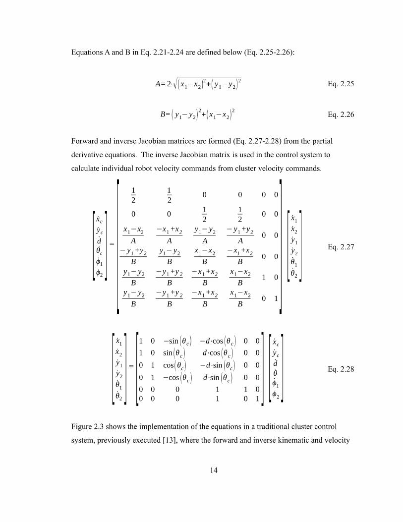
Equations A and B in Eq. 2.21-2.24 are defined below (Eq. 2.25-2.26):

A= 2⋅√(x1−x2)2+( y1−y2)2 Eq. 2.25

B= ( y1− y2)2+(x1−x2)

2Eq. 2.26

Forward and inverse Jacobian matrices are formed (Eq. 2.27-2.28) from the partial

derivative equations. The inverse Jacobian matrix is used in the control system to

calculate individual robot velocity commands from cluster velocity commands.

[xc

yc

dθc

ϕ1ϕ2

] = [12

12

0 0 0 0

0 012

12

0 0

x1−x2A

−x1+x2

A

y1− y2A

− y1+y2

A0 0

− y1+y2

B

y1− y2B

x1−x2B

−x1+x2

B0 0

y1− y2B

−y1+y 2

B

−x1+x2

B

x1−x2B

1 0

y1− y2B

−y1+y 2

B

−x1+x2

B

x1−x2B

0 1

] [x1x2y1y2θ1θ2

] Eq. 2.27

[x1x2y1y2θ1θ2

] = [1 0 −sin (θc) −d⋅cos (θc) 0 0

1 0 sin (θc) d⋅cos (θc) 0 0

0 1 cos(θc) −d⋅sin (θc) 0 0

0 1 −cos (θc) d⋅sin (θc) 0 0

0 0 0 1 1 00 0 0 1 0 1

] [xc

yc

dθϕ1ϕ2

] Eq. 2.28

Figure 2.3 shows the implementation of the equations in a traditional cluster control

system, previously executed [13], where the forward and inverse kinematic and velocity

14

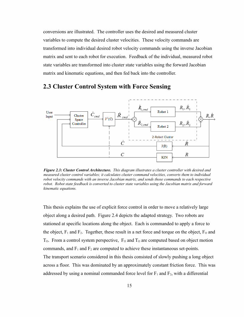
conversions are illustrated. The controller uses the desired and measured cluster

variables to compute the desired cluster velocities. These velocity commands are

transformed into individual desired robot velocity commands using the inverse Jacobian

matrix and sent to each robot for execution. Feedback of the individual, measured robot

state variables are transformed into cluster state variables using the forward Jacobian

matrix and kinematic equations, and then fed back into the controller.

2.3 Cluster Control System with Force Sensing

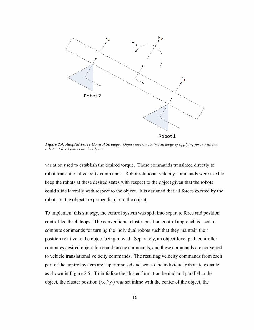
This thesis explains the use of explicit force control in order to move a relatively large

object along a desired path. Figure 2.4 depicts the adapted strategy. Two robots are

stationed at specific locations along the object. Each is commanded to apply a force to

the object, F1 and F2. Together, these result in a net force and torque on the object, FO and

TO. From a control system perspective, FO and TO are computed based on object motion

commands, and F1 and F2 are computed to achieve these instantaneous set-points.

The transport scenario considered in this thesis consisted of slowly pushing a long object

across a floor. This was dominated by an approximately constant friction force. This was

addressed by using a nominal commanded force level for F1 and F2, with a differential

15

Figure 2.3: Cluster Control Architecture. This diagram illustrates a cluster controller with desired and measured cluster control variables; it calculates cluster command velocities, converts them to individual robot velocity commands with an inverse Jacobian matrix, and sends those commands to each respective robot. Robot state feedback is converted to cluster state variables using the Jacobian matrix and forward kinematic equations.

variation used to establish the desired torque. These commands translated directly to

robot translational velocity commands. Robot rotational velocity commands were used to

keep the robots at these desired states with respect to the object given that the robots

could slide laterally with respect to the object. It is assumed that all forces exerted by the

robots on the object are perpendicular to the object.

To implement this strategy, the control system was split into separate force and position

control feedback loops. The conventional cluster position control approach is used to

compute commands for turning the individual robots such that they maintain their

position relative to the object being moved. Separately, an object-level path controller

computes desired object force and torque commands, and these commands are converted

to vehicle translational velocity commands. The resulting velocity commands from each

part of the control system are superimposed and sent to the individual robots to execute

as shown in Figure 2.5. To initialize the cluster formation behind and parallel to the

object, the cluster position (Cxc,Cyc) was set inline with the center of the object, the

16

Figure 2.4: Adapted Force Control Strategy. Object motion control strategy of applying force with two robots at fixed points on the object.

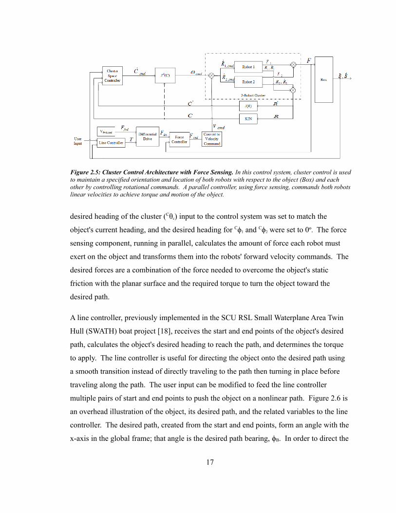
desired heading of the cluster (Cθc) input to the control system was set to match the

object's current heading, and the desired heading for Cϕ1 and Cϕ2 were set to 0º. The force

sensing component, running in parallel, calculates the amount of force each robot must

exert on the object and transforms them into the robots' forward velocity commands. The

desired forces are a combination of the force needed to overcome the object's static

friction with the planar surface and the required torque to turn the object toward the

desired path.

A line controller, previously implemented in the SCU RSL Small Waterplane Area Twin

Hull (SWATH) boat project [18], receives the start and end points of the object's desired

path, calculates the object's desired heading to reach the path, and determines the torque

to apply. The line controller is useful for directing the object onto the desired path using

a smooth transition instead of directly traveling to the path then turning in place before

traveling along the path. The user input can be modified to feed the line controller

multiple pairs of start and end points to push the object on a nonlinear path. Figure 2.6 is

an overhead illustration of the object, its desired path, and the related variables to the line

controller. The desired path, created from the start and end points, form an angle with the

x-axis in the global frame; that angle is the desired path bearing, ϕB. In order to direct the

17

Figure 2.5: Cluster Control Architecture with Force Sensing. In this control system, cluster control is usedto maintain a specified orientation and location of both robots with respect to the object (Box) and each other by controlling rotational commands. A parallel controller, using force sensing, commands both robots linear velocities to achieve torque and motion of the object.

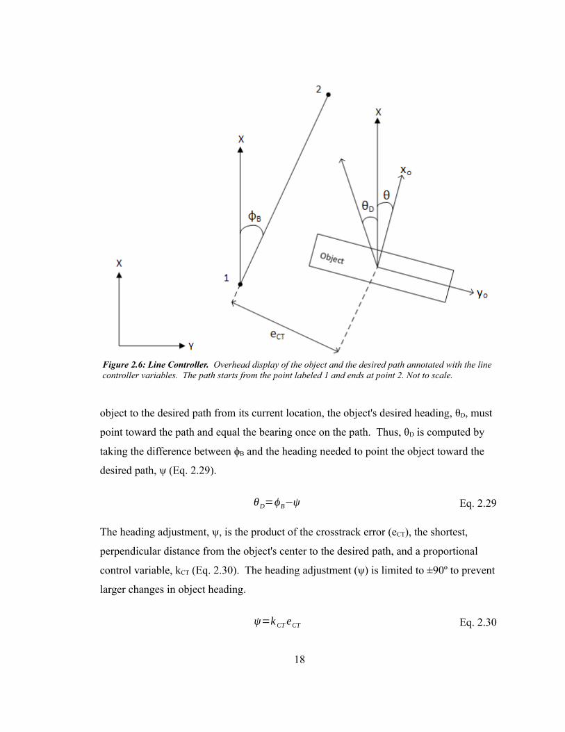
object to the desired path from its current location, the object's desired heading, θD, must

point toward the path and equal the bearing once on the path. Thus, θD is computed by

taking the difference between ϕB and the heading needed to point the object toward the

desired path, ψ (Eq. 2.29).

θD=ϕB−ψ Eq. 2.29

The heading adjustment, ψ, is the product of the crosstrack error (eCT), the shortest,

perpendicular distance from the object's center to the desired path, and a proportional

control variable, kCT (Eq. 2.30). The heading adjustment (ψ) is limited to ±90º to prevent

larger changes in object heading.

ψ=k CT eCT Eq. 2.30

18

Figure 2.6: Line Controller. Overhead display of the object and the desired path annotated with the line controller variables. The path starts from the point labeled 1 and ends at point 2. Not to scale.

A proportional control equation was developed to calculate torque, TO, from the desired

and actual object heading, θO, (Eq. 2.31) with the proportional gain, kH.

TO=k H (θD−θO) Eq. 2.31

The desired torque is converted into the forces needed from each robot to turn and move

the object. Forces are converted into velocity commands. The sum of the velocity

commands and values necessary to overcome the object's static friction, Vfwd,cmd, are the

desired robot velocities. The forward velocity commands derived from force sensing

combined with the rotational commands of the cluster controller create an effective

planar object manipulator. Further research could explore adjusting the location the

robots push on the object for more efficient turning and manipulation of the object's

position.

19

3 Experimental TestbedThis chapter describes the components of the experiment area and the two-robot system

that controls the position of an object in an indoor, planar workspace. The experimental

testbed was developed with fellow graduate student Jackson Arcade.

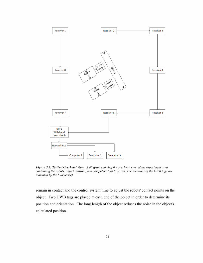
3.1 System Overview

Two robots and a large, rectangular object are placed in an area surrounded by a series of

eight Ultra Wideband (UWB) receivers, creating a rectangular workspace approximately

13 m. by 19 m. A network of computers processes sensor data and controls the robots

using MATLAB®. Equipment mounted on each robot are two, parallel, wireless

communications systems, microcontrollers, a force sensing system, and two UWB tags.

Two UWB tags are mounted to the rectangular object. Figure 3.1 is a photo of the

experiment area containing the robots, the object, and some UWB receivers. Figure 3.2

illustrates an overhead view of the general location of each component in the lab area.

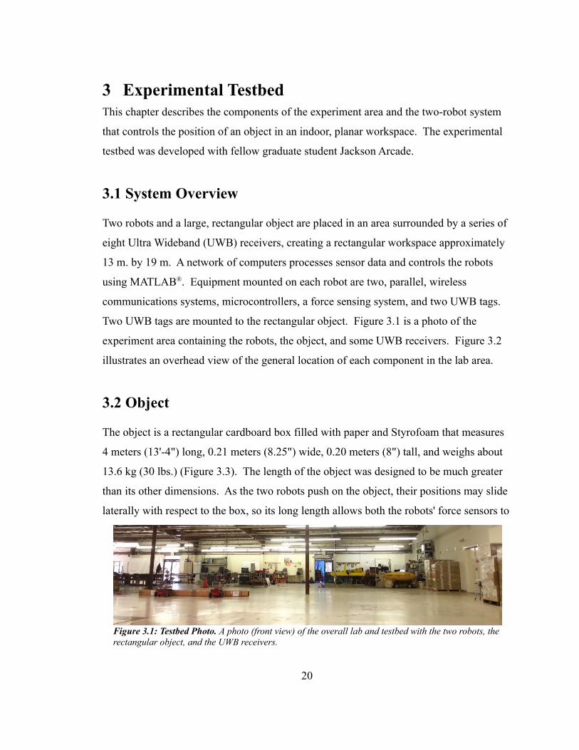
3.2 Object

The object is a rectangular cardboard box filled with paper and Styrofoam that measures

4 meters (13'-4") long, 0.21 meters (8.25") wide, 0.20 meters (8") tall, and weighs about

13.6 kg (30 lbs.) (Figure 3.3). The length of the object was designed to be much greater

than its other dimensions. As the two robots push on the object, their positions may slide

laterally with respect to the box, so its long length allows both the robots' force sensors to

20

Figure 3.1: Testbed Photo. A photo (front view) of the overall lab and testbed with the two robots, therectangular object, and the UWB receivers.

remain in contact and the control system time to adjust the robots' contact points on the

object. Two UWB tags are placed at each end of the object in order to determine its

position and orientation. The long length of the object reduces the noise in the object's

calculated position.

21

Figure 3.2: Testbed Overhead View. A diagram showing the overhead view of the experiment area containing the robots, object, sensors, and computers (not to scale). The locations of the UWB tags are indicated by the * (asterisk).

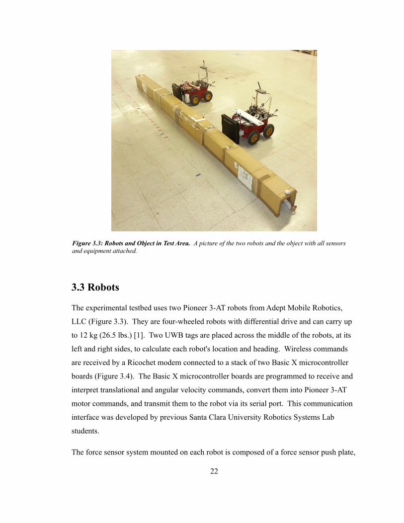
3.3 Robots

The experimental testbed uses two Pioneer 3-AT robots from Adept Mobile Robotics,

LLC (Figure 3.3). They are four-wheeled robots with differential drive and can carry up

to 12 kg (26.5 lbs.) [1]. Two UWB tags are placed across the middle of the robots, at its

left and right sides, to calculate each robot's location and heading. Wireless commands

are received by a Ricochet modem connected to a stack of two Basic X microcontroller

boards (Figure 3.4). The Basic X microcontroller boards are programmed to receive and

interpret translational and angular velocity commands, convert them into Pioneer 3-AT

motor commands, and transmit them to the robot via its serial port. This communication

interface was developed by previous Santa Clara University Robotics Systems Lab

students.

The force sensor system mounted on each robot is composed of a force sensor push plate,

22

Figure 3.3: Robots and Object in Test Area. A picture of the two robots and the object with all sensors and equipment attached.

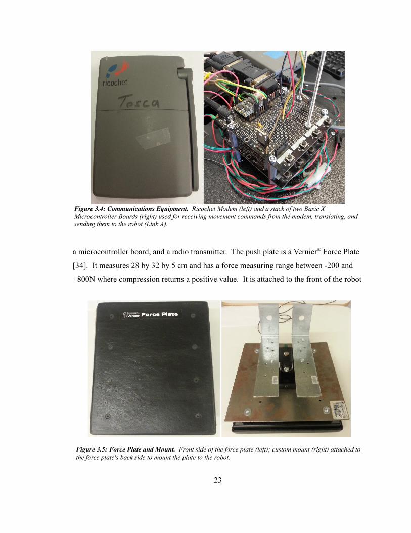
a microcontroller board, and a radio transmitter. The push plate is a Vernier® Force Plate

[34]. It measures 28 by 32 by 5 cm and has a force measuring range between -200 and

+800N where compression returns a positive value. It is attached to the front of the robot

23

Figure 3.4: Communications Equipment. Ricochet Modem (left) and a stack of two Basic X Microcontroller Boards (right) used for receiving movement commands from the modem, translating, and sending them to the robot (Link A).

Figure 3.5: Force Plate and Mount. Front side of the force plate (left); custom mount (right) attached to the force plate's back side to mount the plate to the robot.

with a custom mount, allowing for limited rotation about an axis parallel to the z-axis

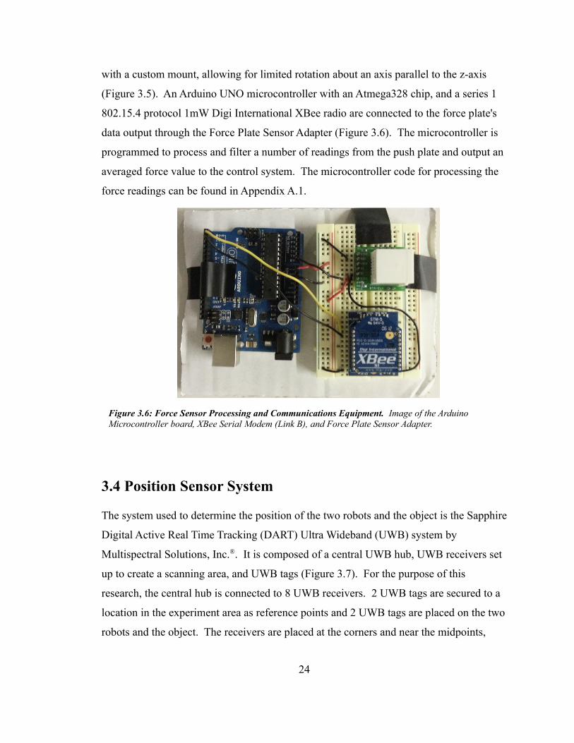
(Figure 3.5). An Arduino UNO microcontroller with an Atmega328 chip, and a series 1

802.15.4 protocol 1mW Digi International XBee radio are connected to the force plate's

data output through the Force Plate Sensor Adapter (Figure 3.6). The microcontroller is

programmed to process and filter a number of readings from the push plate and output an

averaged force value to the control system. The microcontroller code for processing the

force readings can be found in Appendix A.1.

3.4 Position Sensor System

The system used to determine the position of the two robots and the object is the Sapphire

Digital Active Real Time Tracking (DART) Ultra Wideband (UWB) system by

Multispectral Solutions, Inc.®. It is composed of a central UWB hub, UWB receivers set

up to create a scanning area, and UWB tags (Figure 3.7). For the purpose of this

research, the central hub is connected to 8 UWB receivers. 2 UWB tags are secured to a

location in the experiment area as reference points and 2 UWB tags are placed on the two

robots and the object. The receivers are placed at the corners and near the midpoints,

24

Figure 3.6: Force Sensor Processing and Communications Equipment. Image of the Arduino Microcontroller board, XBee Serial Modem (Link B), and Force Plate Sensor Adapter.

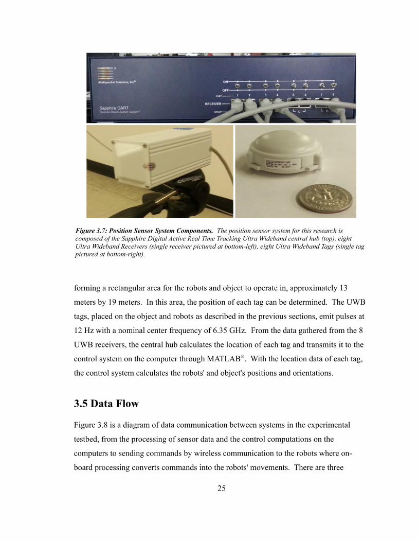
forming a rectangular area for the robots and object to operate in, approximately 13

meters by 19 meters. In this area, the position of each tag can be determined. The UWB

tags, placed on the object and robots as described in the previous sections, emit pulses at

12 Hz with a nominal center frequency of 6.35 GHz. From the data gathered from the 8

UWB receivers, the central hub calculates the location of each tag and transmits it to the

control system on the computer through MATLAB®. With the location data of each tag,

the control system calculates the robots' and object's positions and orientations.

3.5 Data Flow

Figure 3.8 is a diagram of data communication between systems in the experimental

testbed, from the processing of sensor data and the control computations on the

computers to sending commands by wireless communication to the robots where on-

board processing converts commands into the robots' movements. There are three

25

Figure 3.7: Position Sensor System Components. The position sensor system for this research is composed of the Sapphire Digital Active Real Time Tracking Ultra Wideband central hub (top), eight Ultra Wideband Receivers (single receiver pictured at bottom-left), eight Ultra Wideband Tags (single tag pictured at bottom-right).

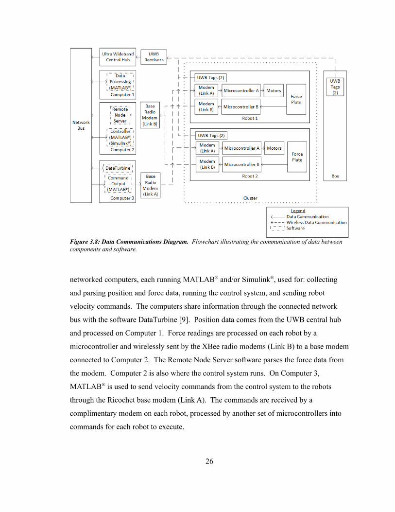
networked computers, each running MATLAB® and/or Simulink®, used for: collecting

and parsing position and force data, running the control system, and sending robot

velocity commands. The computers share information through the connected network

bus with the software DataTurbine [9]. Position data comes from the UWB central hub

and processed on Computer 1. Force readings are processed on each robot by a

microcontroller and wirelessly sent by the XBee radio modems (Link B) to a base modem

connected to Computer 2. The Remote Node Server software parses the force data from

the modem. Computer 2 is also where the control system runs. On Computer 3,

MATLAB® is used to send velocity commands from the control system to the robots

through the Ricochet base modem (Link A). The commands are received by a

complimentary modem on each robot, processed by another set of microcontrollers into

commands for each robot to execute.

26

Figure 3.8: Data Communications Diagram. Flowchart illustrating the communication of data between components and software.

4 Experiment

The performance of the cluster control system with force sensing, to manipulate the

position of an object in two dimensions, was characterized by running a set of

experiments. To test the control system, it was given a linear and circular trajectory path

to follow in the 13 by 19 meter test area. This chapter reviews the key results collected

from performing these experiments.

4.1 Linear Path

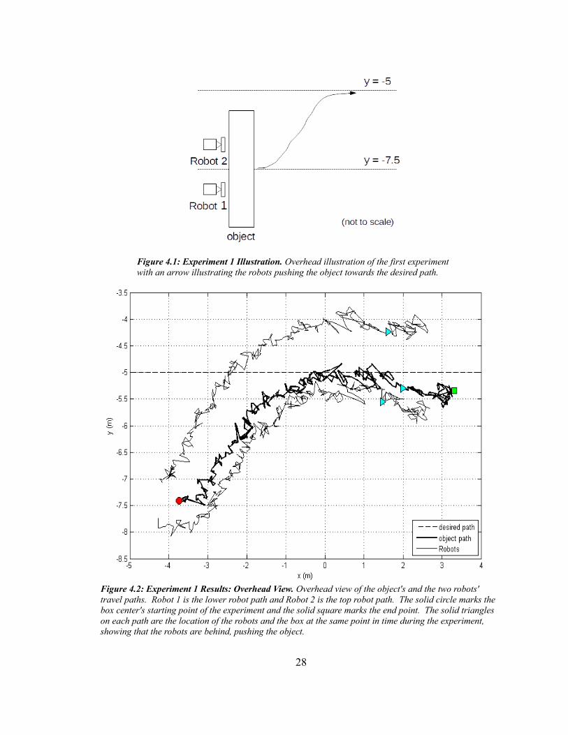
The first experiment was to offset the object and robots from a desired straight line path

and observe the control system command the robots to push the object on a trajectory

toward and onto the desired path. The path was a straight, horizontal line, crossing the y-

axis at y=-5; it served as a step input into the system. The object started in the third

quadrant, near the y=-7.5 horizontal line, pointing in a parallel direction to the desired

path. The control system was tuned to shorten the response time of the system to display

its effectiveness in reaching the desired path within the area allotted. Figure 4.1 is a

notional illustration of the experiment setup with an example trajectory along which the

robots would push the object to reach the desired path. Figure 4.2 displays the overhead

view of the experimental results; the information displayed is the desired path (y=-5), the

measured object (center's) path, and the robots' paths. The robots are set at the

approximate desired starting point with respect to the object.

As the robots push the object from left to right, they successfully push it toward the

desired path. Toward the end of this experiment, the center of the object gets closer to

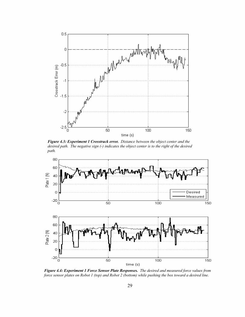
Robot 1 due to the box sliding. Figure 4.3 displays the crosstrack error between the

object center and the desired path. This clearly shows the the controller effectively

pushed the object toward the desired path. The object settled at the desired path within

100 seconds of the start of the experiment with an RMS error of approximately 0.3 m.

The RMS error is on the order of the ±0.3 m. position error reported in the

27

28

Figure 4.1: Experiment 1 Illustration. Overhead illustration of the first experiment with an arrow illustrating the robots pushing the object towards the desired path.

Figure 4.2: Experiment 1 Results: Overhead View. Overhead view of the object's and the two robots' travel paths. Robot 1 is the lower robot path and Robot 2 is the top robot path. The solid circle marks the box center's starting point of the experiment and the solid square marks the end point. The solid triangles on each path are the location of the robots and the box at the same point in time during the experiment, showing that the robots are behind, pushing the object.

29

Figure 4.3: Experiment 1 Crosstrack error. Distance between the object center and the desired path. The negative sign (-) indicates the object center is to the right of the desired path.

Figure 4.4: Experiment 1 Force Sensor Plate Responses. The desired and measured force values from force sensor plates on Robot 1 (top) and Robot 2 (bottom) while pushing the box toward a desired line.

characterization of the UWB system [5]. Figure 4.4 displays the desired and measured

force sensor plate readings during the experiment. Robot 1 is the robot on the right side

of the object's center. Looking at the desired forces of both plates, Robot 1's desired

forces are higher than Robot 2's desired forces to turn the object left toward the desired

path y=-5 line, then become even to push the object straight on the desired path. The

measured force data is noisy.

4.2 Circular Trajectory Path

In the second experiment, the robots were programmed to push the object onto a

30

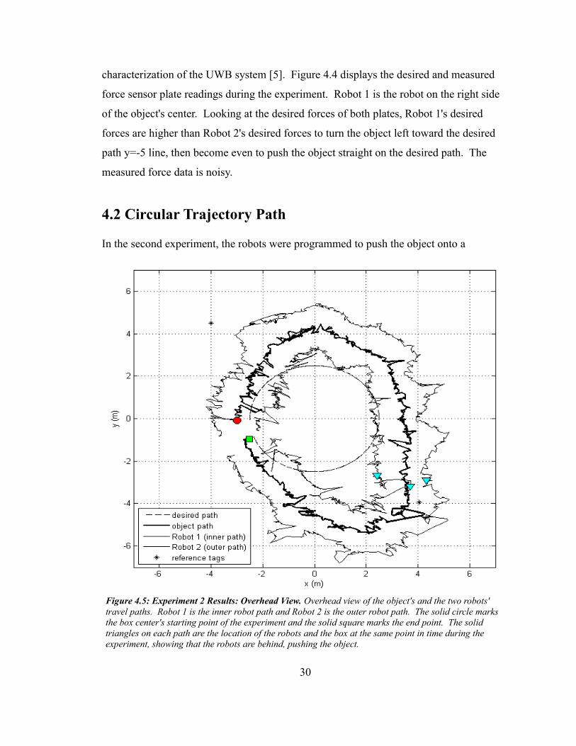
Figure 4.5: Experiment 2 Results: Overhead View. Overhead view of the object's and the two robots' travel paths. Robot 1 is the inner robot path and Robot 2 is the outer robot path. The solid circle marks the box center's starting point of the experiment and the solid square marks the end point. The solid triangles on each path are the location of the robots and the box at the same point in time during the experiment, showing that the robots are behind, pushing the object.

trajectory path of a circle with a 2.5 m radius from the origin of the experiment area. To

do this, a path generator updated the desired trajectory based on the object's current

position and the desired path. The overhead plot in Figure 4.5, shows an excerpt of the

robots’ and the object’s desired and measured paths. The robots were able to push the

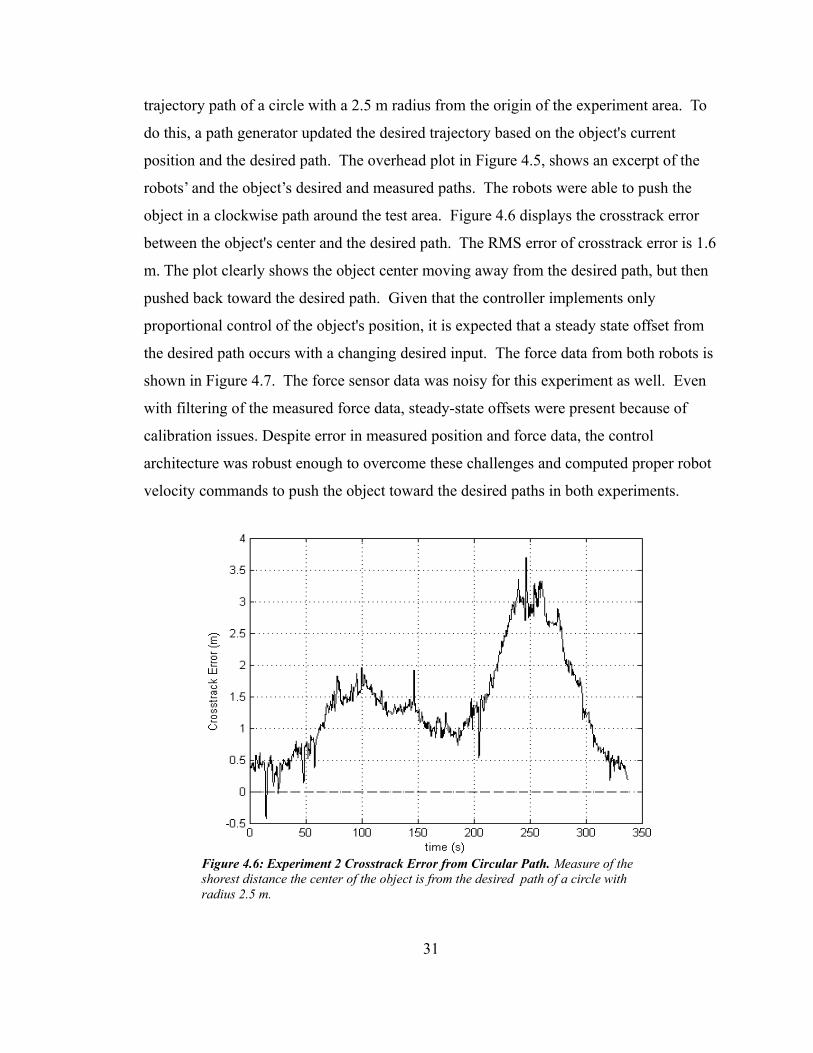
object in a clockwise path around the test area. Figure 4.6 displays the crosstrack error

between the object's center and the desired path. The RMS error of crosstrack error is 1.6

m. The plot clearly shows the object center moving away from the desired path, but then

pushed back toward the desired path. Given that the controller implements only

proportional control of the object's position, it is expected that a steady state offset from

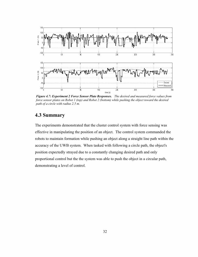
the desired path occurs with a changing desired input. The force data from both robots is

shown in Figure 4.7. The force sensor data was noisy for this experiment as well. Even

with filtering of the measured force data, steady-state offsets were present because of

calibration issues. Despite error in measured position and force data, the control

architecture was robust enough to overcome these challenges and computed proper robot

velocity commands to push the object toward the desired paths in both experiments.

31

Figure 4.6: Experiment 2 Crosstrack Error from Circular Path. Measure of the shorest distance the center of the object is from the desired path of a circle with radius 2.5 m.

4.3 Summary

The experiments demonstrated that the cluster control system with force sensing was

effective in manipulating the position of an object. The control system commanded the

robots to maintain formation while pushing an object along a straight line path within the

accuracy of the UWB system. When tasked with following a circle path, the object's

position expectedly strayed due to a constantly changing desired path and only

proportional control but the the system was able to push the object in a circular path,

demonstrating a level of control.

32

Figure 4.7: Experiment 2 Force Sensor Plate Responses. The desired and measured force values from force sensor plates on Robot 1 (top) and Robot 2 (bottom) while pushing the object toward the desired path of a circle with radius 2.5 m.

5 Conclusion

The objective of this research project was to demonstrate object manipulation control

using a combination of position control and force-sensing in a multirobot system. In

order to accomplish this, a force sensor plate was added to the front of two Pioneer 3-AT

wheeled robots, and the university Robotics Systems Laboratory's multirobot position

control method, cluster control, was modified to include force-sensing. A decoupled

strategy was implemented in the velocity commands of the two robots. Angular velocity

commands for the robots came from the cluster space position controller and the linear

velocity commands were calculated based on data from the force-sensing component of

the controller. These two controllers were wrapped around by a simple object controller

for path keeping.

This research has successfully demonstrated object manipulation using the cluster control

method modified with force-sensing. Results presented in this thesis show a successful

performance of the control system to push the object toward desired trajectory paths of a

straight line and a circle. The robots, spaced apart, pushed an object from the same side

with their attached force plate sensor. Adding force-sensing to the control system

allowed for measured interaction between robots and the object, leading to better control

in object manipulation.

5.1 Future Work

To improve and take this method for object manipulation further, parts of the system

hardware can be made more robust. One direct improvement that can be made is further

calibration of the position and force sensor systems. Increasing accuracy can lead to

better manipulation of the object. Another option would be to use other sensors for

collecting data. For example, a digital compass could replace robot heading data and

reduce the number of RFID tags used. The control system can also be expanded by

developing it into a full hybrid position and force controller. Instead of the decoupling of

33

the linear and angular velocity commands, as presented in this research, a method of

selection can be implemented that would compute a combination of velocity commands

from both the position and force control loops. M.A. Neumann is currently developing

such a hybrid position and force controller. He has also implemented hardware

improvements by preloading and taring the force sensor plates for more accurate data

[26].

Object manipulation using a hybrid position (cluster control method) and force controller

can be expanded in many ways. One of the next steps could be altering the contact

position of the robots to move the object more efficiently. Currently, the robots are set at

positions evenly spaced apart from the center of the object. To turn the object, a torque is

applied by one robot applying more force on the object than the other. By varying the

robots' contact positions on the object they can make more efficient turns; energy

expended by the robots can be minimized and the amount time needed to get the object

on the desired path can be reduced. Additionally, the cluster control method is flexible to

incorporate more robots into its architecture. More complex objects can also be

introduced (e.g. angled objects, objects with hinged joints, etc.). Through the use of state

machines, the control system architecture can be expanded so the robot formation can

autonomously approach, transport, and disengage from an object. Eventually, the control

system could be adapted for environments beyond the indoor testbed such as the marine

environment.

This research is a step towards the greater goal of coordinated, multiple robot

manipulators autonomously manipulating objects with dynamic control. The object could

vary in size, mass, and shape and a system would have the capability to determine the

best parameters for moving said object. Parameters could include the number of robots

necessary to move the object, the most effective path to the desired goal, and how the

robots should approach and exert force on the object to move it to the goal. With

continued development, multirobot object manipulation could be applied to real world

applications in fields of construction, transportation, and more with improved safety and

efficiency.

34

References

1. Adept Technology, Inc. (2012 Aug 13). Pioneer 3-AT [Online]. Available:

http://www.mobilerobots.com/ResearchRobots/P3AT.aspx

2. M. Agnew, P. Dal Canto, C. Kitts, C., and S. Li, "Cluster Space Control of Aerial

Robots," presented at IEEE/ASME Int. Conf. on Advanced Intelligent

Mechatronics. July 2010. [Online]. Available:

http://ieeexplore.ieee.org/xpl/login.jsp?tp=&arnumber=5695814&url=http%3A

%2F%2Fieeexplore.ieee.org%2Fxpls%2Fabs_all.jsp%3Farnumber%3D5695814

3. J. Arcade, “Phase Object Transport Using a Multi-Robot System,” C. Kitts, Adv.,

M.S. thesis, Dept. Mech. Eng., Santa Clara Univ., Santa Clara, CA, 2014.

4. R. G. Brown and J. S. Jennings, “A pusher/steerer model for strongly cooperative

mobile robot manipulation,” in Proc. 1995 IEEE/RSJ Int. Conf. Intell. Robots

Syst. Human Robot Interaction Coop. Robots, Pittsburgh, PA, 1995, vol. 3, pp.

562–568. doi: 10.1109/IROS.1995.525941 Available:

http://ieeexplore.ieee.org/stamp/stamp.jsp?

tp=&arnumber=525941&isnumber=11434

5. J. Cashbaugh, A. Mahacek, C. Kitts, C. Zempel and A. Sherban, "Quadrotor

testbed development and preliminary results," in 2015 IEEE Aerospace

Conference, Big Sky, MT, 2015, pp. 1-12. doi: 10.1109/AERO.2015.7118909

Available: http://ieeexplore.ieee.org/stamp/stamp.jsp?


6. M. Y. Chow, S. Chiaverini and C. Kitts, "Guest Editorial Introduction to the

Focused Section on Mechatronics in Multirobot Systems," in IEEE/ASME

Transactions on Mechatronics, vol. 14, no. 2, pp. 133-140, April 2009. doi:

10.1109/TMECH.2009.2014462 Available:



7. G. Eoh, J.D. Jeon, J. S. Choi and B. H. Lee, “Multi-robot Cooperative Formation

35

http://www.mobilerobots.com/ResearchRobots/P3AT.aspx

http://ieeexplore.ieee.org/stamp/stamp.jsp?tp=&arnumber=4803788&isnumber=4814791






http://ieeexplore.ieee.org/xpl/login.jsp?tp=&arnumber=5695814&url=http%3A%2F%2Fieeexplore.ieee.org%2Fxpls%2Fabs_all.jsp%3Farnumber%3D5695814


for Overweight Object Transportation,” in 2001 IEEE/SICE International

Symposium on System Integration (SII), Kyoto, 2011, pp. 726–731. doi:

10.1109/SII.2011.6147538 Available: http://ieeexplore.ieee.org/stamp/stamp.jsp?


8. J. Fink, M.A. Hsieh, and V. Kumar, “Multi-Robot Manipulation via Caging in

Environments with Obstacles,” in 2008 IEEE Int. Conf. Robot. Autom., Pasadena,

CA, 2008, vol. 8, pp. 1471–1476. doi: 10.1109/ROBOT.2008.4543409 Available:



9. T. Fountain. (2012 Aug. 13). Open Source Data Turbine Initiative. [Online].

Available: http://www.dataturbine.org/

10. B. P. Gerkey and M. J. Matarić, "Pusher-watcher: An approach to fault-tolerant

tightly-coupled robot coordination," in Proc. 2002 of the IEEE Int. Conf. on

Robotics and Automation (Cat. No. 02CH37292), 2002. vol. 1, pp. 464-469. doi:

10.1109/ROBOT.2002.1013403 Available:



11. Y. Hu, L. Wang, J. Liang, T. Wang, “Cooperative box-pushing with multiple

autonomous robotic fish in underwater environment," in IET Control Theory &

Applications, vol. 5, no. 17, pp. 2015–2022, Nov. 17 2011. doi: 10.1049/iet-

cta.2011.0018 Available: http://ieeexplore.ieee.org/stamp/stamp.jsp?


12. T. L.Huntsberger, A. Trebi-Ollennu, H. Aghazarian, P. S. Schenker, P. Pirjanian,

H. D. Nayar, "Distributed Control of Multi-Robot Systems Engaged in Tightly

Coupled Tasks," in Autonomous Robots, vol. 17. 2004, pp. 79-92.

13. R. Ishizu, “The Design, Simulation and Implementation of Multi-Robot

Collaborative Control from the Cluster Perspective,” C. Kitts, Adv., M.S. thesis,

Dept. Elect. Eng., Santa Clara Univ., Santa Clara, CA, 2005.

14. S. Y. Jung and M. A. Goodrich, "Multi-robot perimeter-shaping through mediator-

based swarm control," in 2013 16th International Conference on Advanced

36









Robotics (ICAR), Montevideo, 2013, pp. 1-6. doi: 10.1109/ICAR.2013.6766522

Available: http://ieeexplore.ieee.org/stamp/stamp.jsp?


15. O. Khatib, “A unified approach for motion and force control of robot

manipulators: The operational space formulation,” IEEE J. Robot. Autom., vol. 3,

no. 1, pp. 43–53, Feb 1987. doi: 10.1109/JRA.1987.1087068 Available:



16. C. Kitts and I. Mas, “Cluster Space Specification and Control of Mobile

Multirobot System,” in IEEE/ASME Transactions on Mechatronics, vol. 14, no. 2,

pp. 207–218, April 2009 doi: 10.1109/TMECH.2009.2013943 Available:



17. C. Kitts, P. Mahacek, T. Adamek and I. Mas, "Experiments in the control and

application of Automated Surface Vessel fleets," OCEANS'11 MTS/IEEE KONA,

Waikoloa, HI, 2011, pp. 1-7. doi: 10.23919/OCEANS.2011.6106976 Available:



18. C. A. Kitts, et al., “Field operation of a robotic SWATH boat for shallow water

bathymetric characterization,” in Journal of Field Robotics, vol. 29, no. 6, pp.

924-938, Nov./Dec. 2012.

19. C.R. Kube, H. Zhang, “The Use of Perceptual Cues in Multi-Robot Box-

Pushing,” in Proc. IEEE Intl. Conf. Robot. Autom., Minneapolis, MN, 1996, vol.

3, pp. 2085–2090. doi: 10.1109/ROBOT.1996.506178 Available:



20. J. Li, T. Dong, and Y. Li, “Research on Task Allocation in Multiple Logistics

Robots Based on an Improved Ant Colony Algorithm,” in 2016 Int. Conf. Robot.

Autom. Eng. (ICRAE), Jeju, 2016, vol. 16, pp. 17–20. doi:

10.1109/ICRAE.2016.7738780 Available:

37













21. P. Mahacek, I. Mas, and C. Kitts, "Cluster Space Control of Autonomous Surface

Vessels Utilizing Obstacle Avoidance and Shielding Techniques," presented at

IEEE/OES Autonomous Underwater Vehicles. Sep 2010. [Online]. Available:

http://ieeexplore.ieee.org/xpl/login.jsp?tp=&arnumber=5779668&url=http%3A

%2F%2Fieeexplore.ieee.org%2Fxpls%2Fabs_all.jsp%3Farnumber%3D5779668

22. P. Mahacek, C. A. Kitts and I. Mas, "Dynamic Guarding of Marine Assets

Through Cluster Control of Automated Surface Vessel Fleets," in IEEE/ASME

Transactions on Mechatronics, vol. 17, no. 1, pp. 65-75, Feb 2012. doi:

10.1109/TMECH.2011.2174376F Available:



23. P. Mahacek, “Design and Cluster Space Control of Two Autonomous Surface

Vessels,” C. Kitts, Adv., M.S. thesis, Dept. Mech. Eng., Santa Clara Univ., Santa

Clara, CA, May 2013.

24. I. Mas and C. A. Kitts, “Object manipulation using cooperative mobile multi-

robot systems,” in Proc. World Congr. Eng. Comput. Sci., 2012, vol. 1, pp. 324–

329.

25. M. J. Matarić, M. Nilsson, and K. T. Simsarin, “Cooperative multi-robot box-

pushing,” in Proc. 1995 IEEE/RSJ Int. Conf. Intell. Robot. Syst.: Human Robot

Interaction Coop. Robots, Pittsburgh, PA, 1995, vol. 3, pp. 556–561. doi:

10.1109/IROS.1995.525940 Available: http://ieeexplore.ieee.org/stamp/stamp.jsp?


26. M. A. Neumann and C. A. Kitts, "A Hybrid Multirobot Control Architecture for

Object Transport," in IEEE/ASME Transactions on Mechatronics, vol. 21, no. 6,

pp. 2983-2988, Dec. 2016. doi: 10.1109/TMECH.2016.2580539

27. G.A.S. Pereira, V. Kumar, M.F.M Campos, “Decentralized Algorithms for Multi-

Robot Manipulation via caging,” in The International Journal of Robotics

Research, vol. 23, no. 7-8, pp.783–795, 2004. doi: 10.1177/0278364904045477

38









28. E.T. Smith, M. G. Feemster and J. M. Esposito, "Swarm Manipulation Of An

Unactuated Surface Vessel," in 2007 39th Southeastern Symposium on System

Theory, Macon, GA, 2007, pp. 16-20. doi: 10.1109/SSST.2007.352309 Available:



29. P. Song and V. Kumar, “A potential field based approach to multi-robot

manipulation,” in Proc. 2002 IEEE Int. Conf. Robot. Autom. (Cat.

No.02CH37292), Washington, DC, 2002, vol. 2, pp. 1217–1222. doi:

10.1109/ROBOT.2002.1014709 Available:



30. B.J. Stephens and C.G. Atkenson, “Dynamic Balance Force Control for

Compliant Humanoid Robots,” in 2010 IEEE/RSJ International Conference on

Intelligent Robots and Systems, Taipei, 2010, pp. 1248–1255. doi:

10.1109/IROS.2010.5648837 Available:



31. A. Stroupe, A. Okon, M. Robinson, T. Huntsberger, H. Aghazarian, E.

Baumgartner, “Sustainable cooperative robotic technologies for human outpost

infrastructure construction and maintenance,” in Springer Science + Business

Media, LLC, April 2006, p. 113–123.

32. D. Sun and J.K. Mills, “Manipulating rigid payloads with multiple robots using

compliant grippers,” in IEEE/ASME Trans. Mechatronics, vol. 7, no. 1, pp. 23–

34, Mar. 2002. doi: 10.1109/3516.990884 Available:



33. J. Tan, N. Xi, “Integrated Sensing and Control of Mobile Manipulators,” in Proc.

2001 IEEE/RSJ Int. Conf. Intell. Robots and Syst. Expanding the Societal Role of

Robotics in the Next Millennium (Cat. No.01CH37180), Maui, HI, 2001, vol. 2,

pp. 865–870. doi: 10.1109/IROS.2001.976277 Available:

39











34. Vernier. (2013, Aug 13). Force Plate [Online]. Available:

http://www.vernier.com/products/sensors/force-sensors/fp-bta/

35. Z. Wang, Y. Hirata, and K. Kosuge, “Control Multiple Mobile Robots for Object

Caging and Manipulation,” in Proc. 2003 IEEE/RSJ Int. Conf. Intell. Robot. Syst.

(IROS 2003) (Cat. No.03CH37453), 2003, vol. 2, pp. 1751–1756. doi:

10.1109/IROS.2003.1248897 Available:



36. D. Zhang, L. Wang, J. Yu, M. Tan, “Coordinated transport by Multiple

Biomimetic Robotic Fish in Underwater Environment,” in IEEE Transactions on

Control Systems Technology, vol. 15, no. 4, pp. 658–671, July 2007. doi:

10.1109/TCST.2007.899153 Available:



40





http://www.vernier.com/products/sensors/force-sensors/fp-bta/



Appendix

A.1 Arduino code for collecting and filtering force data

/*--------------------------------------------------------

Program that takes in voltage input from pin A0, 0-5V,

converts it to a count value between 0 and 1023.

Data is using a continuous average of all the data points.

Continuously reads in data into an array. Every 250 points

it will calculate an average, a variance, eliminate outliers

that are a (or many) standard deviation(s), depending on

variable "rule," from the average and will update the average.

At the same time, every 500 milliseconds, it will recalculate the

average. Via experimental data, the count value is put through a

calibration curve to produce a force value.

Converts the numerical value to a string and printed out

serially.

//Matthew Chin

//Michael Vlahos

//updated 2013.05.17

--------------------------------------------------------*/

#include <TimedAction.h>

int analogInPin=A0;

int n = -1;

float mem[251];

int k=0;

double totAverage=0;

double totVar = 0;

double stdDev = 0;

int m = 0;

int rule = 3; //# of standard deviations away I want to eliminate data.

double Force = 0;

TimedAction timedAction = TimedAction(500,outputAverage);

A-1

void setup()

{

Serial.begin(9600);

}

void loop()

{

n=n+1;

if (n>250)

{

n=0;

calAverage();

}

mem[n]=analogRead(analogInPin)/10.0;

k++;

timedAction.check();

}

void calAverage()

{

int sum = 0;

double average = 0;

for (int i = 0; i<250; i++)

{

sum = sum+mem[i];

}

// Serial.println(k);

average = (totAverage*(m)+sum)/(m+250);

// totAverage=average;

// Serial.println(double(average));

double var = 0;

for (int i = 0; i<250; i++)

{

A-2

var = (var*(i)+pow( (mem[i]-average),2) )/(i+1);

}

totVar= totVar*((k-250.0)/(k)) + 250*var/(k);

// Serial.println(double(var));

double dev = pow(totVar,0.5);

for (int i = 0; i<250; i++) //new average

{

if ( (mem[i]>=(average-rule*dev)) && (mem[i]<=(average+rule*dev)) )

{

totAverage = (totAverage*m + mem[i])/(m+1);

m=m+1;

}

}

// Serial.println(float(totAverage/10));

}

void outputAverage()

{

calAverage();

// stdDev = pow(totVar,0.5);

// Serial.println(mem[249]);

/* Multiply totAverage by a factor of 10 to bring it to the correct scale

and 1.24(counts)-182.48 is calibration curve. */

Force = totAverage*12.4-182.48;

/* Uncomment and write Serial.print("!") to robot 1's Arduino

and uncomment and write Serial.print("_") to Arduino on robot 2 */

// Serial.print("!"); // Print the tag ! for sensor 1

// Serial.print("_"); // Print the tag _ for sensor 2

Serial.println(Force);

/* If move calibration curve to control system, then only output

calculated average. */

// Serial.println(totAverage*10);

A-3

/* Testing program outputs */

// Serial.println(stdDev);

// Serial.println(m);

// Serial.println(k);

k=0;

m=0;

totAverage=0;

totVar=0;

Force = 0;

// Serial.println(" ");

// Serial.println(n);

}

A-4

A.2 Simulink Model of the Control System

A-5

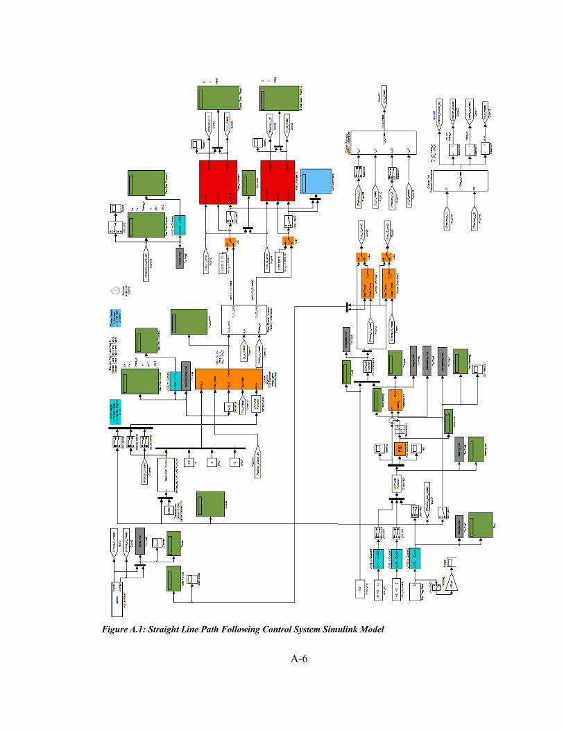
A-6

Figure A.1: Straight Line Path Following Control System Simulink Model

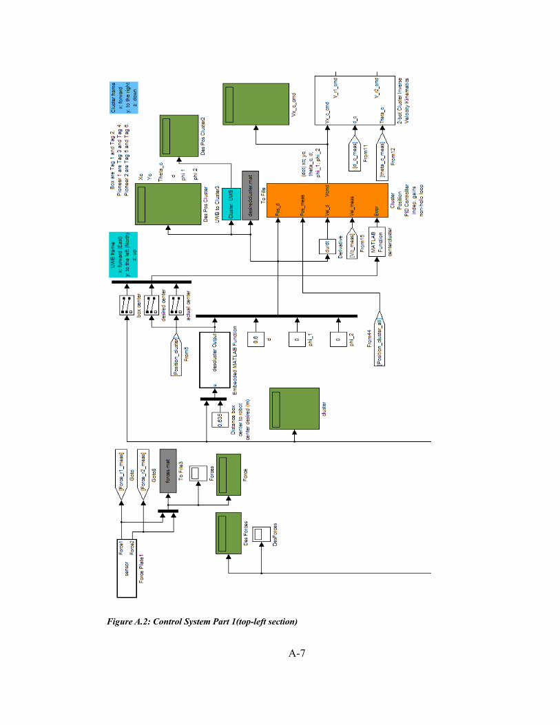
A-7

Figure A.2: Control System Part 1(top-left section)

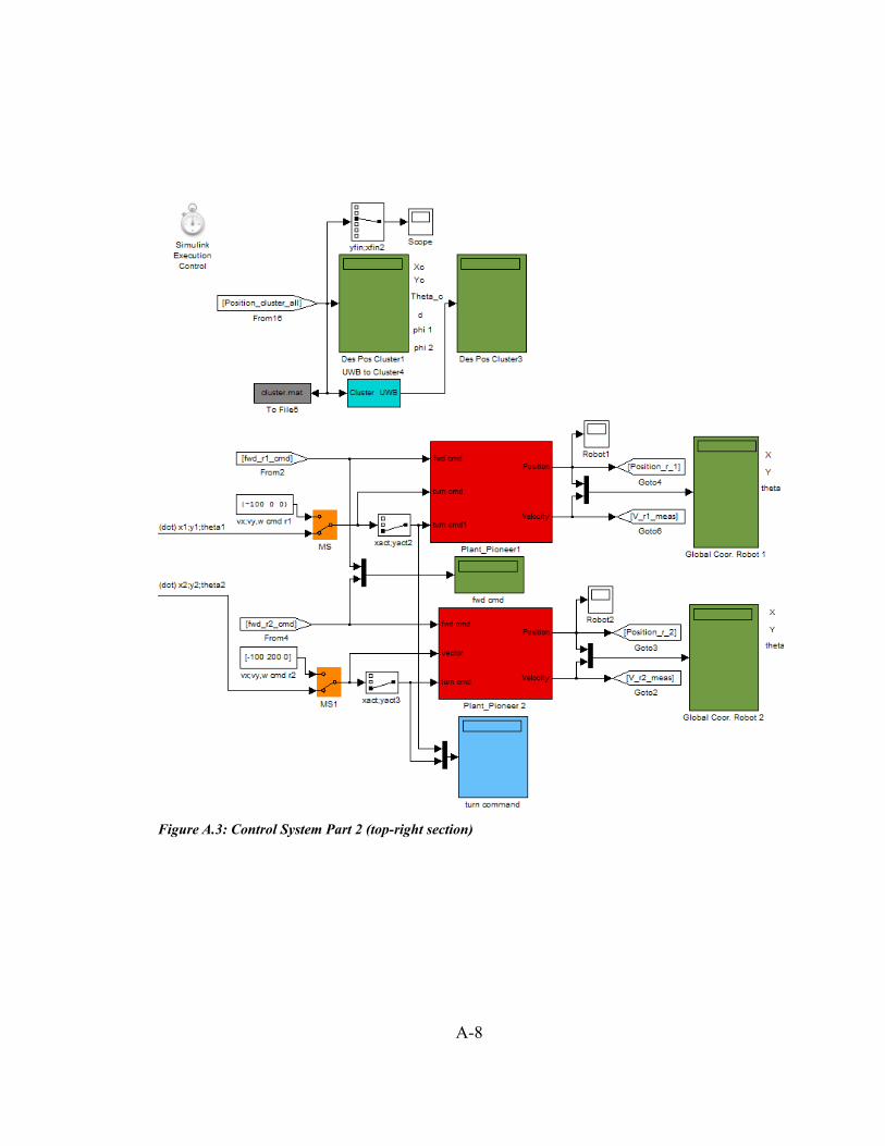
A-8

Figure A.3: Control System Part 2 (top-right section)

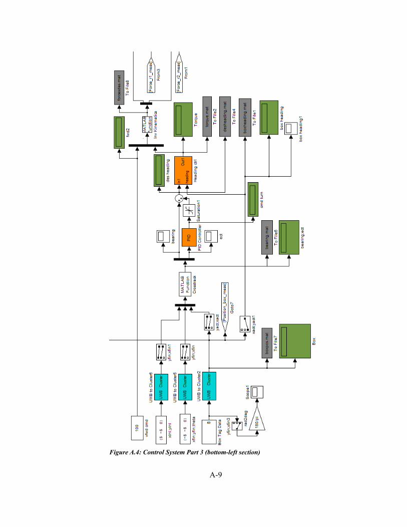
A-9

Figure A.4: Control System Part 3 (bottom-left section)

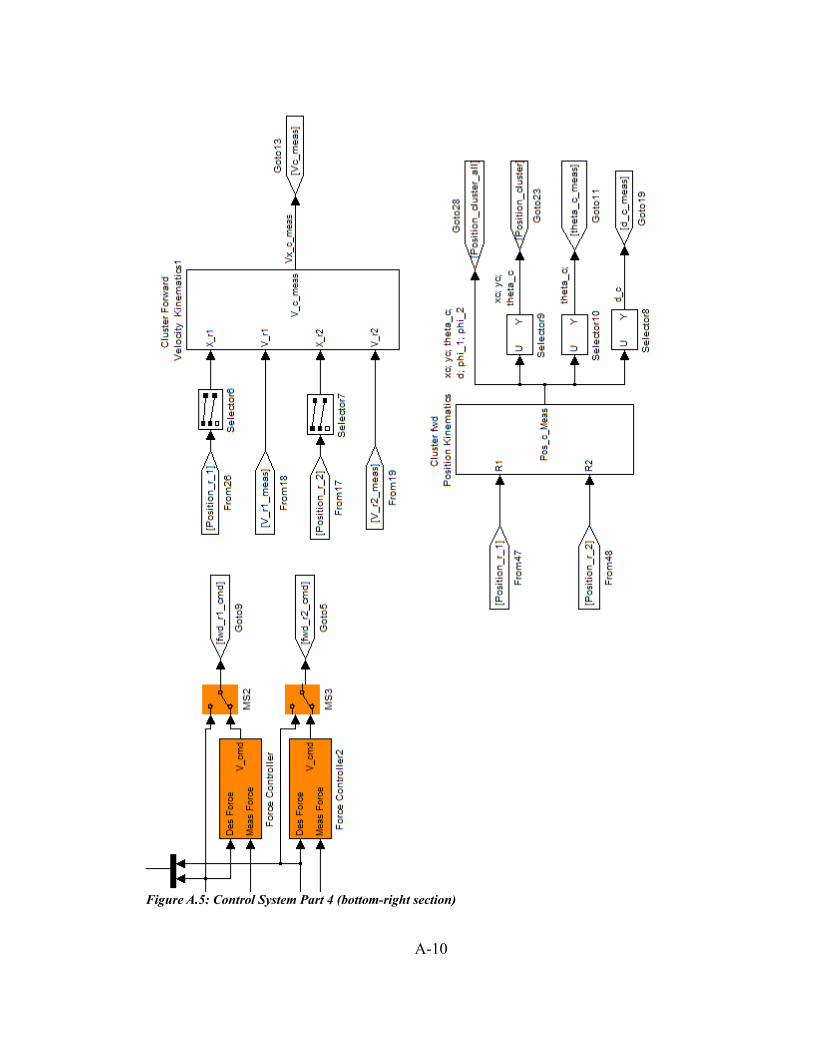
A-10

Figure A.5: Control System Part 4 (bottom-right section)

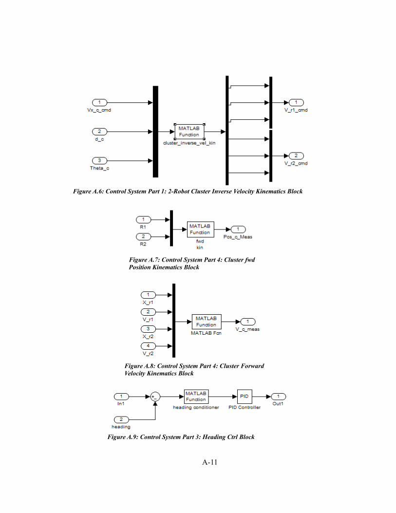
A-11

Figure A.6: Control System Part 1: 2-Robot Cluster Inverse Velocity Kinematics Block

Figure A.8: Control System Part 4: Cluster Forward Velocity Kinematics Block

Figure A.7: Control System Part 4: Cluster fwd Position Kinematics Block

Figure A.9: Control System Part 3: Heading Ctrl Block

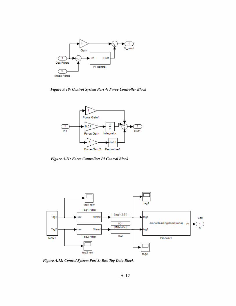
A-12

Figure A.11: Force Controller: PI Control Block

Figure A.12: Control System Part 3: Box Tag Data Block

Figure A.10: Control System Part 4: Force Controller Block

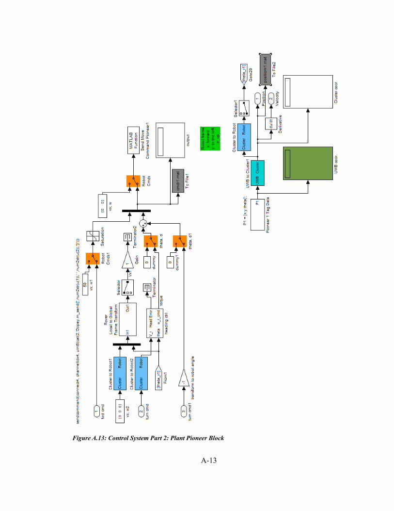
A-13

Figure A.13: Control System Part 2: Plant Pioneer Block

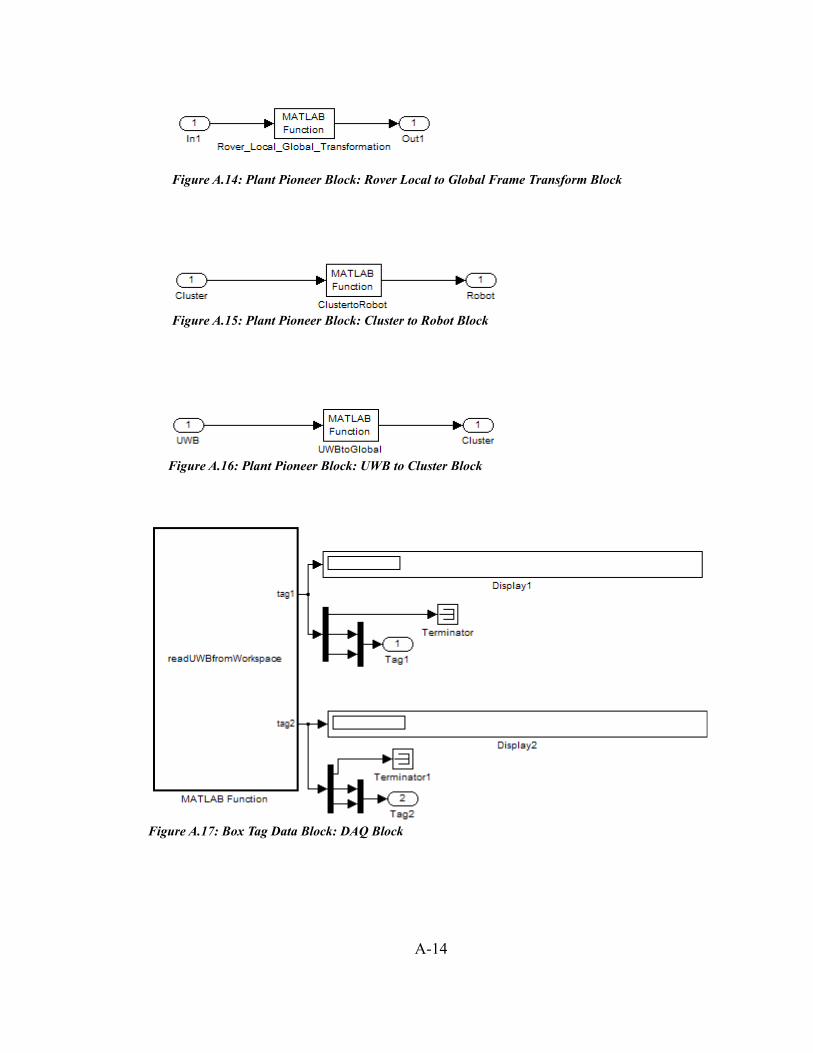
A-14

Figure A.17: Box Tag Data Block: DAQ Block

Figure A.16: Plant Pioneer Block: UWB to Cluster Block

Figure A.14: Plant Pioneer Block: Rover Local to Global Frame Transform Block

Figure A.15: Plant Pioneer Block: Cluster to Robot Block

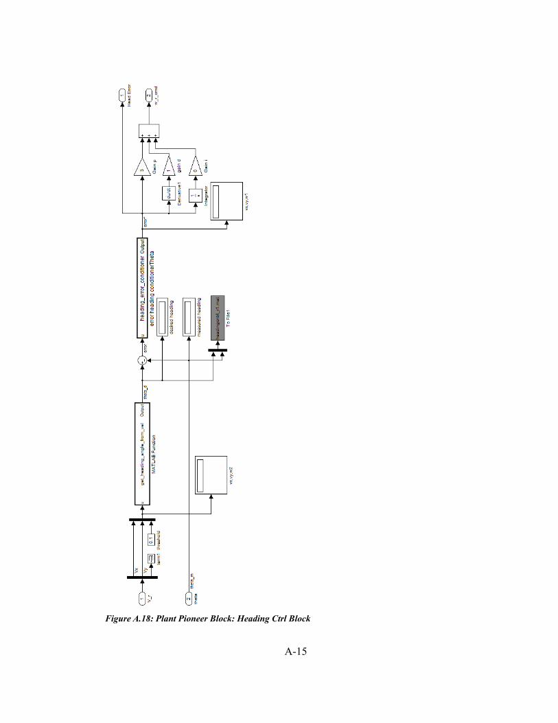
A-15

Figure A.18: Plant Pioneer Block: Heading Ctrl Block

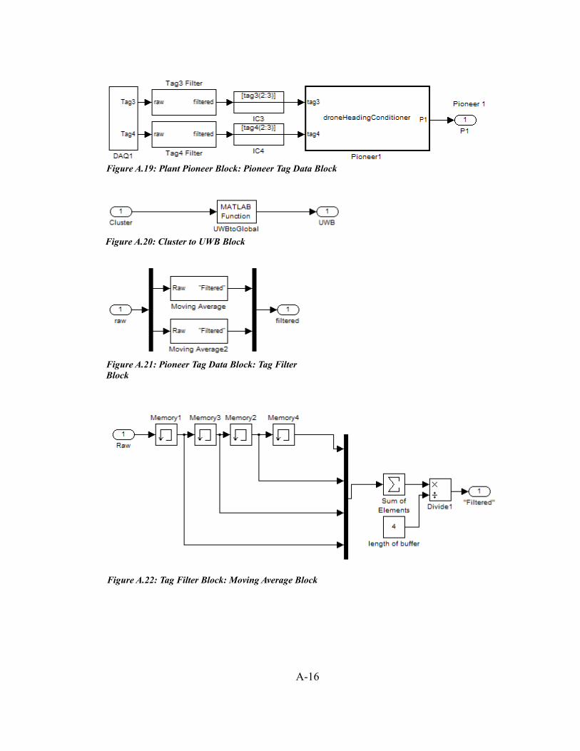
A-16

Figure A.19: Plant Pioneer Block: Pioneer Tag Data Block

Figure A.21: Pioneer Tag Data Block: Tag Filter Block

Figure A.22: Tag Filter Block: Moving Average Block

Figure A.20: Cluster to UWB Block

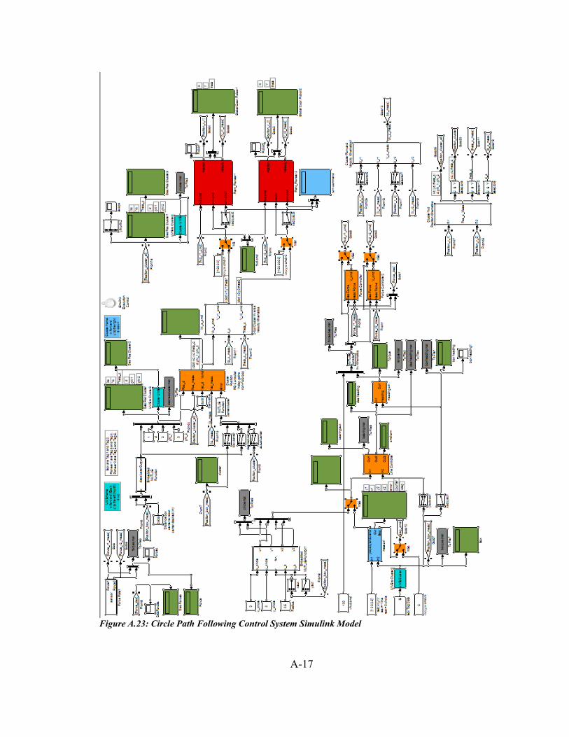
A-17

Figure A.23: Circle Path Following Control System Simulink Model

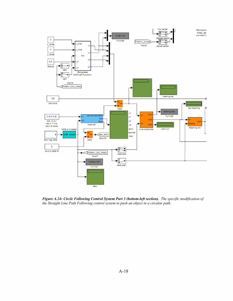
A-18

Figure A.24: Circle Following Control System Part 3 (bottom-left section). The specific modification of the Straight Line Path Following control system to push an object in a circular path.

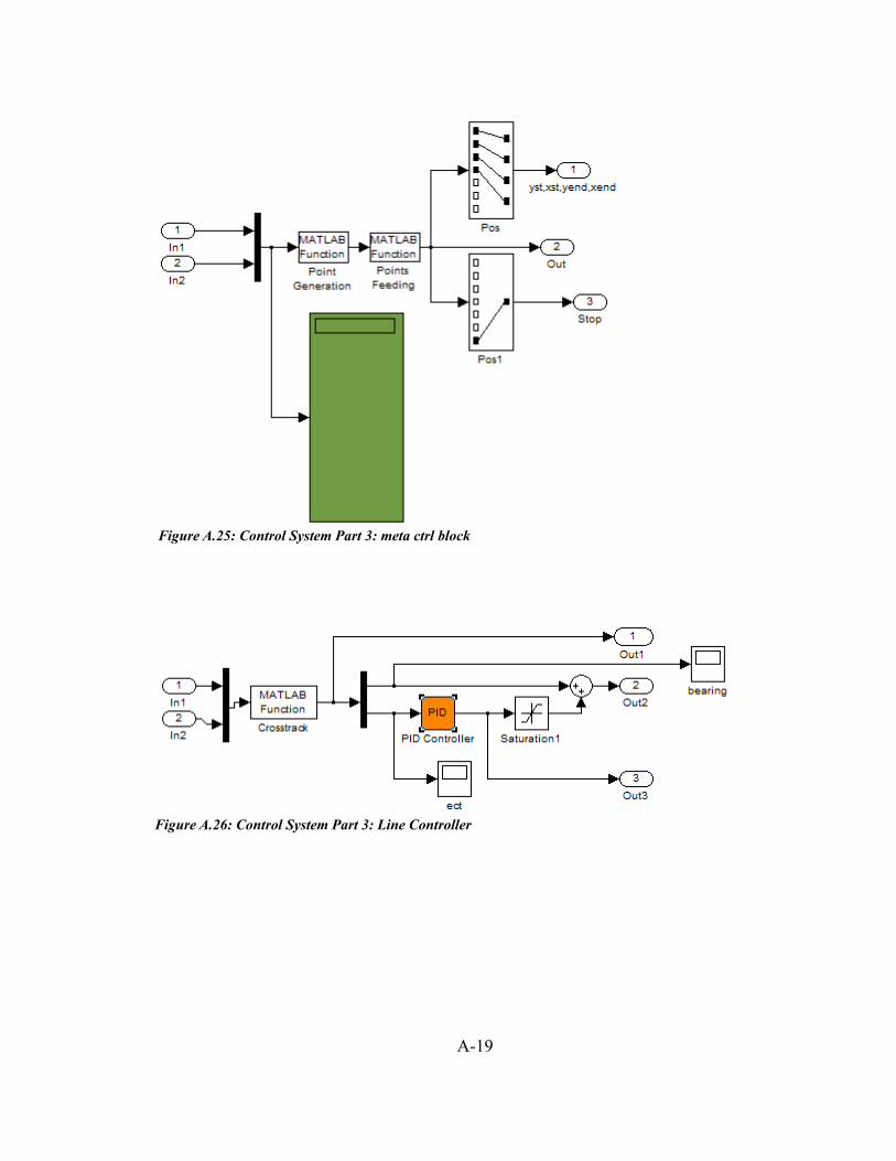
A-19

Figure A.25: Control System Part 3: meta ctrl block

Figure A.26: Control System Part 3: Line Controller

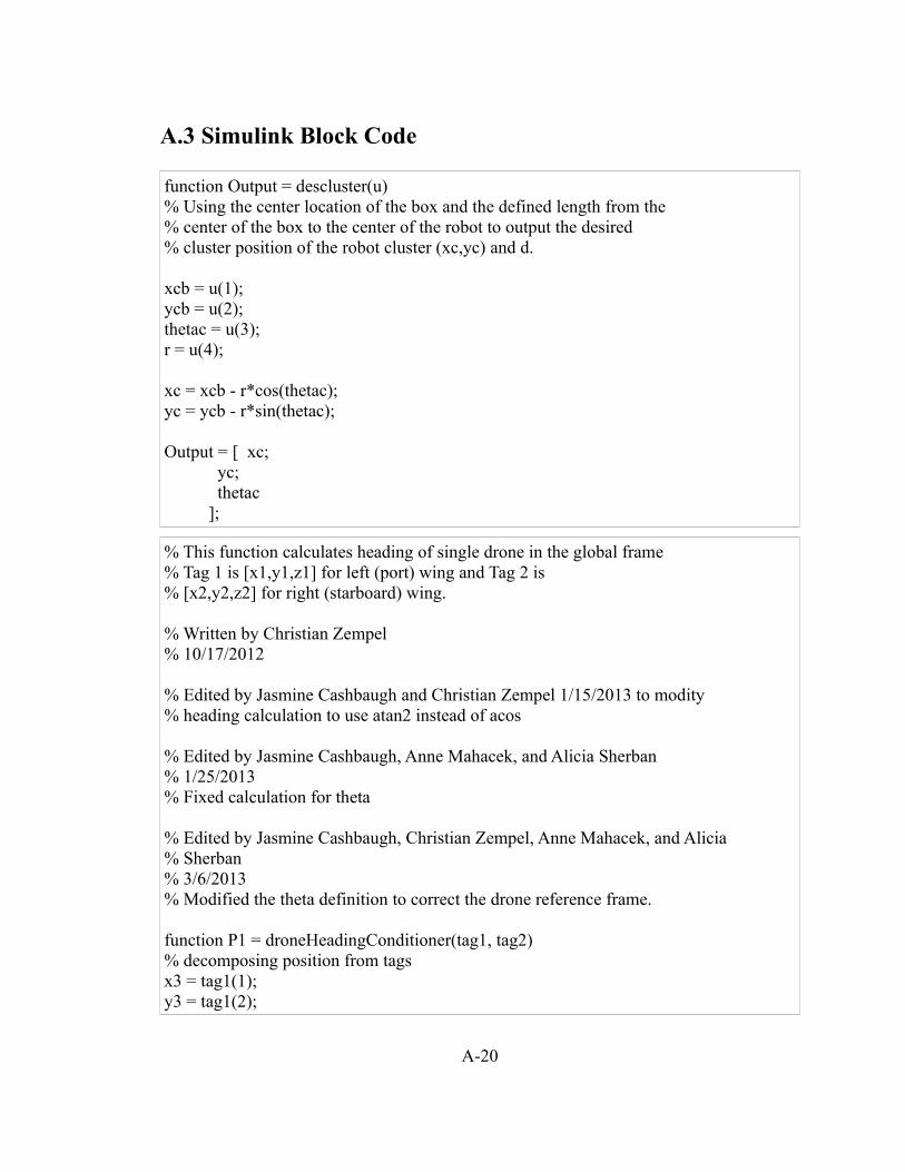
A.3 Simulink Block Code

function Output = descluster(u)% Using the center location of the box and the defined length from the% center of the box to the center of the robot to output the desired% cluster position of the robot cluster (xc,yc) and d.

xcb = u(1);ycb = u(2);thetac = u(3);r = u(4);

xc = xcb - r*cos(thetac);yc = ycb - r*sin(thetac);

Output = [ xc; yc; thetac ];

% This function calculates heading of single drone in the global frame% Tag 1 is [x1,y1,z1] for left (port) wing and Tag 2 is% [x2,y2,z2] for right (starboard) wing.

% Written by Christian Zempel% 10/17/2012

% Edited by Jasmine Cashbaugh and Christian Zempel 1/15/2013 to modity% heading calculation to use atan2 instead of acos

% Edited by Jasmine Cashbaugh, Anne Mahacek, and Alicia Sherban% 1/25/2013% Fixed calculation for theta

% Edited by Jasmine Cashbaugh, Christian Zempel, Anne Mahacek, and Alicia% Sherban% 3/6/2013% Modified the theta definition to correct the drone reference frame.

function P1 = droneHeadingConditioner(tag1, tag2)% decomposing position from tagsx3 = tag1(1);y3 = tag1(2);

A-20

% z3 = tag1(3);

x4 = tag2(1);y4 = tag2(2);% z4 = tag2(3);

% Calculate Drone's Center of Gravity [x,y,z] in Global Frame

x = (x3+x4)/2;y = (y3+y4)/2;% z = (z3+z4)/2;

% Calculate Drone's Heading [theta] in Global Frame

yd_vec = [(x3-x4) (y3-y4)]'; % vector connecting two tagsyd_uvec = yd_vec./sqrt((x3-x4)^2 + (y3-y4)^2); % y-drone unit vector

yg_uvec = [0 1]'; % define y-global unit vectorxg_uvec = [1 0]';

% Calculate theta.%Theta (heading of drone)is angle between x-global and x-drone equal to the%angle between y-drone and negative y-globaltheta = atan2(yd_uvec(1),-yd_uvec(2));

P1 = [x y theta]';

function Output = heading_error_conditioner(u)% This function produces heading angle error conditioning so there's no jump% at angular discontinuities% Converts error: [-360:-180] to [0:180], [-180:180] % to [180:180], and [180:360] to [-180:0].% arguments: u = [angular_error]% output: output = [conditioned_angular_error]

%Initialize variablesthreshold=pi;

e = u(1);e=mod(e,2*pi); % Sets e to remainder of angular error divided by 2pi.

% Changes the error from the current pointing direction of the robot to% be the positive equivalent angle error. -360 to -1 changes to 0 to 359.

A-21

% Positive error values stay the same.

if abs(e) > threshold %checks if absolute value of e is greater than pi if e<0 %if error is negative e=e+2*pi; e=min(e,pi+e);

else %if error is positive e=e-2*pi; e=min(e,pi-e); end end

%e=min(e,pi-e); %outputs angular heading in -pi to pi range

Output = e;

function Output = get_heading_angle_from_vel(u)%This function computes the heading angle for a differential drive based on the cluster velocities of robots%threshold is the min vel that outputs a desired heading, otherwise is zero.%arguments: u = [Vx Vy threshold]%output: output = [theta_des]

%Initialize variablesVx = u(1);Vy = u(2);threshold = u(3);vel_mod = sqrt(Vx^2+Vy^2);if vel_mod <= threshold heading=0;else heading=atan2(Vy,Vx);% heading=atan2(Vx,Vy);end

Output = heading;

function Output = get_heading_angle_from_vel(u)%This function computes the heading angle for a differential drive based on the cluster velocities of robots%threshold is the min vel that outputs a desired heading, otherwise is zero.%arguments: u = [Vx Vy threshold]

A-22

%output: output = [theta_des]

%Initialize variablesVx = u(1);Vy = u(2);threshold = u(3);vel_mod = sqrt(Vx^2+Vy^2);if vel_mod <= threshold heading=0;else heading=atan2(Vy,Vx);% heading=atan2(Vx,Vy);end

Output = heading;

function [tag1,tag2] = readUWBfromWorkspace% Function takes in data stream from 'base' workspace, this is the data% being from the UWB through DT. Segregates data stream into 'n' row% matrices, where 'n' is the numberOfTags.

% Function for TWO DRONE ONLY

% Edited by Christian Zempel 3/22/13 to eliminate 'evalin' function which% does not run with simulinktag1 = zeros(1,3);tag2 = zeros(1,3);

coder.extrinsic('evalin');tag1 = evalin('base', 'tag1');tag2 = evalin('base', 'tag2');

function [Force1,Force2] = sensor% Function takes in data stream from 'base' workspace, this is the data% being from the RemoteNodeServer through DT. Continuously updates the% value of the force for 2 force sensors.

Force1=[0];Force2=[0];

coder.extrinsic('evalin')Force1 = evalin('base','Force1');Force2 = evalin('base','Force2');

A-23

Documents

Object Manipulation using a Multirobot Cluster with Force