Embed Size (px)
Citation preview
Object Localization Using
Deformable Templates
Jonathan Michael Spiller
A dissertation submitted to the Faculty of Engineering and the Built Environment,
University of the Witwatersrand, Johannesburg, in fulfilment of the requirements for
the degree of Master of Science in Engineering.
Johannesburg, April 2007

Declaration
I declare that this dissertation is my own, unaided work, except where otherwise ac-
knowledged. It is being submitted for the degree of Master of Science in Engineering in
the University of the Witwatersrand, Johannesburg. It has not been submitted before
for any degree or examination in any other university.
Signed this day of 20
Jonathan Michael Spiller.
i
Summary
Object localization refers to the detection, matching and segmentation of objects in
images. The localization model presented in this paper relies on deformable templates
to match objects based on shape alone. The shape structure is captured by a prototype
template consisting of hand-drawn edges and contours representing the object to be
localized. A multistage, multiresolution algorithm is utilized to reduce the computational
intensity of the search. The first stage reduces the physical search space dimensions
using correlation to determine the regions of interest where a match it likely to occur.
The second stage finds approximate matches between the template and target image at
progressively finer resolutions, by attracting the template to salient image features using
Edge Potential Fields. The third stage entails the use of evolutionary optimization to
determine control point placement for a Local Weighted Mean warp, which deforms the
template to fit the object boundaries. Results are presented for a number of applications,
showing the successful localization of various objects. The algorithm’s invariance to
rotation, scale, translation and moderate shape variation of the target objects is clearly
illustrated.
ii

Acknowledgements
I would like to thank the following people and cat for their assistance throughout
this...ordeal:
Prof. Tshilidzi Marwala, my supervisor, for his moral and financial support, guidance,
insight, inexhaustible (and believe me I tried) patience, and lunch.
My parents, for their love and support, for letting me move back in without paying rent.
Ma, for proofreading this (I know how painful it was...I had to write it), and Dad, for
the car keys.
Evan “Ed” Hurwitz, for sharing a lane with me or letting me solo mid, whichever was
needed.
The folks at Kentron, for funding this research, and for not requiring phone calls (which
I didn’t want to make), or emails (which I didn’t want to send).
Lynx, for keeping me company working late into the night, and for dfttt666666777777777.........
walking across my keyboard.
Charlene, for posing for the pictures. Without you I would have had to break my camera
photographing Ed!
Angelina. Call me.
iii
Preface
This dissertation is presented to the University of the Witwatersrand, Johannesburg,
South Africa, in fulfilment of the requirements of the degree of Master of Science in
Engineering.
The dissertation is entitled “Object Localization Using Deformable Templates,” and
complies with the university’s “paper-model” format. It consists of three chapters, each
of which comprises a standalone paper written for submission to a conference or journal.
These are:
1. J.M. Spiller and T. Marwala, “Object Localization Using Deformable Templates,”
currently (on date of submission of this dissertation) being prepared for submission
as a journal article.
2. J.M. Spiller and T. Marwala, “Evolutionary Algorithms for Warp Control Point
Placement,” submitted to The 2nd International Symposium on Intelligence Com-
putation and Applications, to take place in Wuhan, China, during September 2007.
3. J.M. Spiller and T. Marwala, “Medical Image Segmentation and Localization using
Deformable Templates,” In Proceedings of the International Federation of Medical
and Biological Engineering, 2006, Vol. 14, pp. 2176-2179, Springer-Verlag, Berlin
Heidelberg, Eds. Sun I. Kim and Tae Suk Sah, ISSN: 1727-1983.
A fourth paper, “Object Localization in Aerial Images Using Deformable Templates,” is
currently in the process of being written and has not been included in this document.
iv

An extended abstract for this paper has been submitted to The First International Sym-
posium on Information and Computer Elements, to take place during September 2007
in Kitakyushu, Japan. The paper details an application of the localization algorithm to
aerial and satellite images and includes a section on predicting affine warps for template
instantiations, based on photogrammetry and aerial geometry techniques.
v
Contents
Declaration i
Summary ii
Acknowledgements iii
Preface iv
Contents vi
List of Figures ix
Nomenclature xii
1 Object Localization Using Deformable Templates 1
1 Introduction . . . . . . . . . . . . . . . . . . . . . . . . . . . . . . . . . . . 3
2 Deformable Templates . . . . . . . . . . . . . . . . . . . . . . . . . . . . . 5
2.1 Free-Form Models . . . . . . . . . . . . . . . . . . . . . . . . . . . 6
vi
2.2 Parametric Models . . . . . . . . . . . . . . . . . . . . . . . . . . . 7
3 The Deformation Model . . . . . . . . . . . . . . . . . . . . . . . . . . . . 9
3.1 The Prototype Template . . . . . . . . . . . . . . . . . . . . . . . . 10
3.2 Control Points . . . . . . . . . . . . . . . . . . . . . . . . . . . . . 11
4 The Multistage Algorithm . . . . . . . . . . . . . . . . . . . . . . . . . . . 12
4.1 Stage One - Regions of Interest . . . . . . . . . . . . . . . . . . . . 13
4.2 Stage Two - Multiresolution Matching . . . . . . . . . . . . . . . . 15
4.3 Stage Three - Template Warping . . . . . . . . . . . . . . . . . . . 20
5 Experimental Results . . . . . . . . . . . . . . . . . . . . . . . . . . . . . . 29
5.1 Search Capability . . . . . . . . . . . . . . . . . . . . . . . . . . . . 29
5.2 Template Convergence . . . . . . . . . . . . . . . . . . . . . . . . . 30
5.3 Rotation Invariance . . . . . . . . . . . . . . . . . . . . . . . . . . 30
5.4 Scale Invariance . . . . . . . . . . . . . . . . . . . . . . . . . . . . 31
5.5 Object Tracking . . . . . . . . . . . . . . . . . . . . . . . . . . . . 31
6 Conclusion and Future Work . . . . . . . . . . . . . . . . . . . . . . . . . 32
References 39
2 Evolutionary Algorithms for Warp Control Point Placement 46
1 Introduction . . . . . . . . . . . . . . . . . . . . . . . . . . . . . . . . . . . 47
2 Registration for Object Localization . . . . . . . . . . . . . . . . . . . . . 48
vii
3 Template Warping . . . . . . . . . . . . . . . . . . . . . . . . . . . . . . . 49
4 Evolutionary Algorithms . . . . . . . . . . . . . . . . . . . . . . . . . . . . 50
4.1 Genetic Algorithm . . . . . . . . . . . . . . . . . . . . . . . . . . . 51
4.2 Particle Swarm Optimization . . . . . . . . . . . . . . . . . . . . . 52
4.3 Simulated Annealing . . . . . . . . . . . . . . . . . . . . . . . . . . 52
5 Results . . . . . . . . . . . . . . . . . . . . . . . . . . . . . . . . . . . . . . 53
6 Conclusion . . . . . . . . . . . . . . . . . . . . . . . . . . . . . . . . . . . 55
References 56
3 Medical Image Segmentation and Localization Using Deformable Tem-
plates 57
I Introduction . . . . . . . . . . . . . . . . . . . . . . . . . . . . . . . . . . . 58
II A Model of Deformation . . . . . . . . . . . . . . . . . . . . . . . . . . . . 58
III The Multi-Stage Algorithm . . . . . . . . . . . . . . . . . . . . . . . . . . 58
IV Experimental Results . . . . . . . . . . . . . . . . . . . . . . . . . . . . . . 60
V Conclusion . . . . . . . . . . . . . . . . . . . . . . . . . . . . . . . . . . . 61
References 61
viii
List of Figures
1 Object Localization Using Deformable Templates 1
1 Deformable template model: (a) A prototype template of a Clownfish,
with control points shown. (b) An image containing a Clownfish to be
localized. . . . . . . . . . . . . . . . . . . . . . . . . . . . . . . . . . . . . 10
2 Defining shape: Different instances of objects with the same shape. . . . . 11
3 Finding the regions of interest: (a) Eye template. (b) Face image. (c)
EPF obtained from (b). (d) NCC surface plot. (e) Binary image mask
obtained by thresholding (d). (f) Regions of interest. . . . . . . . . . . . . 16
4 Edge Potential Fields: (a) Base image of Macaw. (b) Base edge map,
σ = 2 . (c) Distance map, σ = 2. (d) Base edge orientation map. . . . . . 17
5 Multiresolution search: (a) Prototype Macaw template. (b) Coarse EPF,
σ = 4. (c) Medium EPF, σ = 2.5. (d) Fine EPF, σ = 1. (e) Final
template match. (f) 5 Coarse EPF matches. (g) 3 Medium EPF matches.
(h) 1 Fine EPF match. . . . . . . . . . . . . . . . . . . . . . . . . . . . . . 20
6 Control point placement: (a) A prototype template of a hand. (b) Base
image of a hand. (c) Template alignment showing initial (red) and opti-
mized (green) control point locations. . . . . . . . . . . . . . . . . . . . . 22
ix
7 LWM warping: (a) A prototype template of a hand. (b) A deformed
template of the hand bending to the right. (c) A deformed template of
the hand bending to the left. (d) Extreme deformation resulting in an
impractical shape. . . . . . . . . . . . . . . . . . . . . . . . . . . . . . . . 28
8 Search capability: (a) Prototype templates of the letters G O L F and
the VW logo. (b) Image of Golf GTI. (c) Medium resolution localization
showing spurious results, E ≈ 0.2. (d) Fine resolution localization, E ≈0.1. (e) Magnification of (c). (f) Magnification of (d). . . . . . . . . . . . 34
9 Template convergence: (a) Image of a Snowy Owl overlayed with the
prototype template, E = 0.459. (b) Coarse resolution template warp, 20
iterations, E = 0.317. (c) Medium resolution template warp, 50 iterations,
E = 0.223. (d) Fine resolution template warp, 100 iterations, E = 0.086. . 35
10 Rotation invariance: (a) Prototype template of windmill blade. (b) Image
of windmill. (c) Localization of windmill blades at orientations around
360◦. (d) Magnified localization of windmill blades. . . . . . . . . . . . . . 36
11 Scale Invariance: (a) Prototype arch template. (b) Image of the Segovia
Aqueduct. (c) Localization of arches at various scales. (d) Magnified
localization of arches. . . . . . . . . . . . . . . . . . . . . . . . . . . . . . 37
12 Object Tracking: (a) Prototype hand template. (b) Frames showing hand
motion. (c) Object tracking of hands within each frame. . . . . . . . . . . 38
2 Evolutionary Algorithms for Warp Control Point Placement 46
1 Average convergence characteristics of GA, PSO and SA. . . . . . . . . . 54
2 Hand warp using GA: Image sequence showing initial to final template
warps at 15 iteration intervals. . . . . . . . . . . . . . . . . . . . . . . . . 54
3 Fish warp using SA: Template warps at 0, 50, 75 iterations and final
template localization. . . . . . . . . . . . . . . . . . . . . . . . . . . . . . . 55
x
4 Owl warp using PSO: Image sequence shows actual implementation of the
localization algorithm at 0, 20, 50 and 100 iterations. . . . . . . . . . . . . 55
3 Medical Image Segmentation and Localization Using Deformable Tem-
plates 57
1 Deformable template matching: (a) A prototype template of a typical
Corpus Callosum shape with control points. (b) MRI base image where
the Corpus Callosum must be localized and segmented. . . . . . . . . . . 58
2 Corpus Callosum MRI images. (a) Original image. (b) Segmented image. 60
3 Segmentation of aneurysms in ultrasound images. . . . . . . . . . . . . . 61
4 MRI lung segmentation. . . . . . . . . . . . . . . . . . . . . . . . . . . . . 61
5 Carpal bone segmentation from x-ray. . . . . . . . . . . . . . . . . . . . . 61
xi

Nomenclature
EPF - Edge Potential Field
LWM - Local Weighted Mean
PSO - Particle Swarm Optimization
GA - Genetic Algorithm
SA - Simulated Annealing
xii
Chapter 1
Object Localization Using Deformable
Templates
This paper forms the main body of the thesis, to which it also lends its name. It is
currently (on date of submission of this dissertation) being prepared for submission as
a journal article. It comprehensively details the template deformation model and the
multistage algorithm, and presents a number of test results highlighting key features of
the localization paradigm.
1
Object Localization UsingDeformable Templates
J.M. Spiller and T. Marwala
Abstract- A new algorithm is presented for localizing objects in images, using de-
formable templates. Prior knowledge of object shape is described by a prototype tem-
plate, which consists of shape-representative contours and edges, as well as a set of
control points for image warping. Computational efficiency is achieved using a mul-
tistage approach to find a match between the deformed template and objects in the
image, by minimizing a cost function between the template and object boundary. The
first stage of the algorithm reduces the physical search space size by determining the re-
gions of interest using cross-correlation between the template and the edges of the image.
A multiresolution paradigm is adopted for the second and third stages. In the second
stage, an adapted hierarchical Chamfer matching scheme is used to find approximate
matches between the template and the image using directional Edge Potential Fields
(EPFs) of progressively higher resolutions. In the third stage, an innovative method
using Particle Swarm Optimization is employed to find optimal control point placement
at each resolution. A Local Weighted Mean (LWM) warp is also employed at this stage
to facilitate a registration that iteratively deforms the template to fit these optimized
points. The dimensionality of possible warp transformations is overcome by minimizing
a cost function that penalizes extreme warps. The algorithm is succesfully applied to a
number of images and the localization results are given, with each test set highlighting
a different aspect of the algorithm.
2
1 Introduction
Object localization refers to the location and retrieval of objects from complex images. It
is a wide-ranging problem that has importance, both as a final outcome and as a prelim-
inary stage, in many image processing and computer vision tasks. Typical applications
include image database retrieval [1–3], object recognition [4,5], image segmentation [6,7]
and registration [8, 9]. In all such localization applications, a priori information in the
form of an inexact model of an object needs to be matched to the objects present in the
base image. This information typically includes properties such as shape, color, texture,
etc.
This paper addresses the problem of localization based on objects’ 2D shape informa-
tion only. It is approached as a process of matching a deformable template to the object
boundary in an input image. Prior knowledge of an object is defined by a binary tem-
plate, which consists of a rough sketch of shape-representative contours and edges, as
well as a set of control points for image warping. This prototype template is not para-
meterized, but complete shape information is contained in the bitmap image. In order
to find objects similar in shape to the template, deformations of the prototype shape are
required. Deformed templates are obtained by shifting the control points to generate
varying parametric warp transforms.
In order to determine a match, a two term objective function is minimized. The first term
measures the potential energy between the object boundary, specified by the deformable
template, and the edges and gradient directions in the base image. During matching,
this term attracts the template toward salient image features. The second term is a
penalty function that penalizes extreme deformations and helps to maintain a likely
shaped template. The localization model minimizes the objective function by iteratively
adjusting the control point positions and then warping to find the lowest energy fit
between the template and edges in the image.
The majority of non-rigid template matching techniques either require initialization near
the final solution, or are too slow for practical use [10]. This is largely attributed to the
fact that the number of possible transformations that can be applied to the template
is very large, resulting in computationally intractable optimization requirements. In
3
contrast, the method presented here is able to quickly find a global optimal solution,
without any initialization. The objective function that is minimized is non-convex, and in
order to find its minima efficiently, a multistage, multiresolution algorithm is employed.
In the first stage, regions of interest are determined by evaluating the 2D correlation
between the template and the image. In the second stage, approximate matches between
the template and the image are found using multiresolution directional EPFs. Template
matches at coarse resolutions are used to initiate matching at finer ones. The final
stage of the algorithm employs an innovative warping method that uses evolutionary
algorithms to determine the placement of control points on the image, and then utilizes a
LWM warp to deform the template to fit these points. Invariance to rotation, translation
and scale is achieved by applying the template at discrete orientations during each stage.
The robustness of the algorithm is illustrated by experimental results showing the ac-
curate detection of deformable shapes even in highly cluttered images. The algorithm
presented here falls under the pattern theoretic model of Grenander [11, 12], and is
based partially on the work of Zhong and Jain [13,14], who have shown that localization
paradigms such as this exhibit a number of important qualities [14]:
• They can match shapes that are curved or polygonal, closed or open, simply or
multiply connected.
• They can retrieve objects based on shape information alone, even in complex im-
ages.
• They can localize objects independent of their location, orientation, size and num-
ber in the image.
• localization is achieved in a computationally efficient manner using a multistage,
multiresolution approach.
The rest of this paper is set out as follows: Section 2 gives a brief review of deformable
templates, discussing their background, different models and applications and the latest
developments in the field. Section 3 defines the template model used by the presented
algorithm. It discusses the prototype template and the control points used for warping.
The multistage algorithm is detailed in Section 4. This section explains the three stages
4
of the matching technique, from the identification of regions of interest, through the
multiresolution search, and lastly the template warping methodology. Section 5 contains
the results for a number of test scenarios, with each experiment highlighting a different
aspect of the algorithm. Finally, Section 6 gives a conclusion and presents a number of
ideas for future work in this field.
2 Deformable Templates
Literature suggests that the first versatile technique for detection of parameterized
shapes was proposed by Hough in 1962 [15]. Templates were described by a set of
parameters such as the slope and intercept of a line. The Hough Transform (HT) trans-
fers points from spatial space into parameter space, and then finds peaks in this new
domain. The method was later improved by Rosenfeld, Ballard and Brown respectively,
to detect shapes described by an analytic curve as well as to incorporate parameters to
translate, rotate, and scale the template. [16–18]. Although it is relatively insensitive
to noise and occlusion, the applicability of the HT is limited by excessive memory and
computational requirements. It is also unreliable when tasked with finding deformed
shapes, i.e. those that differ from the prototype by more complex transformations than
translations, rotation and scale. Full surveys of the HT, its variants and its applications
can be found in [19] and [20].
Deformable templates are refered to as “active” because of their ability to adjust to fit
given data. Models of this type are useful because of their flexibility, and for their abilities
to both impose geometric constraints on a shape, and integrate local image evidence [13].
Because of their wide-ranging application, substantial research on template modeling has
been done in recent years. Current research can be divided into two catagories:
• Free-form models.
• Parametric models.
This section provides a brief literature survey of influential free-form and parametric
template models. A number of pioneering models are presented, as well as some of the
5
latest developments in the field.
2.1 Free-Form Models
Free-form models refer to models where no global structure is specified. Templates
are constrained only by general regularization constraints such as smoothness and/or
connectivity of the boundary. Free-form models are capable of representing any arbitrary
shape, provided these constraints are satisfied. Templates of this kind are typically
attracted to prominent image features by energy functions of some sort.
An early example of a free-form model is the elastic deformable model of [21]. This
method establishes an elastic model of one of the two images to be matched, and then
uses local forces to iteratively warp it towards the other image. In [22], this model
was successfully extended to the 3D scenario. A popular free-form model known as an
active contour was introduced by Kass, Witkin and Terzopoulos in 1988 [23, 24]. They
presented an energy-minimizing spline, known as a “snake”, controlled by a combination
of three forces that induce regularizing constraints to ensure smoothness, attract the
snake to the desired features, and influence its shape if required. One weakness of snake
models, however, is that they operate on local image information only. As such, they are
susceptible to noise, and highly dependent on initial instantiation position. Numerous,
varying provisions have been made to improve the robustness and stability of snakes.
Notably, in [25], Cohen and Cohen introduced an inflationary “balloon” force to expand
or contract the contour. This helped the snake to escape from local minima formed
by spurious, weak image edges. Spline-based template models provide more structure
than snake models. Templates are expressed as linear combinations of functions, such
as B-spline basis, trigonometric basis and wavelets. Chan and Vese developed an active
contour based on curve evolution and level sets to detect boundaries that are not clearly
defined by gradient information [26].
A number of statistical methods have also been used to improve the robustness of tem-
plate matching schemes. The authors of [27] used hierarchical eigen-shapes and Bayesian
inference with Markov Chain Monte Carlo sampling to recover 3D shape and texture
6
of an object, based on a single 2D view. In [28], a Bayesian probability model of im-
age filter-banks, sampled via Monte Carlo methods, was presented to overcome the
requirements of an exhaustive search. B-splines were used in [29] to estimate parametric
deformable contours. The authors formulated the problem in a statistical framework
with the likelihood function being derived from a region-based image model.
Free-form models have been successfully applied to contour detection [23, 25], object
tracking [30] and segmentation tasks [31]. Free-form models, however, do not inherently
contain knowledge about the shapes they are finding. When such knowledge is available,
it can be incorporated into the search using parametric deformable models.
2.2 Parametric Models
Parametric models are controlled using a set of parameters that encode specific shape
characteristics as well as permissible deformations [13]. Models of this type are useful
when specific shape information is known and can be described by the set of parameters.
Parameterization is accomplished in one of two ways: It is done either by constructing a
set of equations defining the curves in the shape, which can then be controlled by varying
the equations’ parameters, or by developing a prototype model and applying parametric
transformations to it in order to obtain different deformations.
In the first instance - curve parameterization - all prior information is captured in analytic
form, by equations that uniquely describe the constituent curves of a shape. As with
free-form models, the curves evolve to fit the evidence by updating their parameters
so as to minimize some curve energy function. In [32], parametric template models
were used to locate road boundaries by searching for pairs of straight, parallel edges in
radar images. In a facial feature detection application, eye and mouth templates were
constructed using circles and parabolic curves and controlled by parameters such as the
radius of the circle and the intercepts and stationary points of the parabolas [33]. The
authors of [34] used elliptical Fourier descriptors to represent open and closed boundaries
with high degrees of freedom, which matched objects in medical images. Distributions
of Fourier coefficients were used to specify likely shapes, while a Bayesian likelihood
was used to estimate the optimal object boundary. A similar scheme was used in [35],
7
but included region homogeneity and edge strength in the likelihood distribution. The
applicability of curve parameterization is limited because shapes need to be well-defined
and representable by a set of curves with a manageably small set of parameters.
In the second instance - prototype template modeling - parameterization is based on the
pattern theory of Grenander [11,12], who developed a framework for representing classes
of similar structure that are able to accommodate certain variability. Models of this type
consist of a prototype template, which describes an overall architecture and shape, as
well as a parametric mapping which governs variation of that shape. Templates are
chosen based on prior knowledge of the shape, usually described by typical, expected or
average shape and may even be learned from a set of training samples. The associated
parametric mapping is chosen to reflect the particular deformations allowed in a specific
application domain.
The basic idea of prototype-based deformable models can be traced back to 1973. In [36],
Fischler and Elshlager used a number of rigid components, held together by springs to
represent a scene. The springs served as constraints on the relative movements of the
components, and the amount by which they stretched also provided a measure of the
cost of a description. Also in 1973, Widrow used a template drawn on a “rubber sheet”
that could be locally stretched to form a specific shape [37].
In [38], the authors used polygons to construct template models of human hands, and
then used Markov processes to obtain variations of the prototype. Also involving hands,
Amit et al [39] represented a prototype hand as an intensity image and used dynamic
programming to obtain template variance. Training samples were used in [40] to compute
the average shape of a class of objects for use as the prototype. The deformations of the
templates were modeled by using linear combinations of eigenvectors obtained from the
variations of the class individuals from the mean template.
More recently, Jain et al [14] used hand-drawn prototype templates, warped using radial
basis functions to match objects in images. A Bayesian framework was adopted, basing
the likelihood of a match on both the expected shape and image evidence. The author
of [10] used triangulated polygons to approximate the boundaries of objects and then
used dual graphs to embed each triangle independently in the image. The accuracy of
8
the match was evaluated based on the log-anisotropy measure of how far each embedding
was from a similarity transform of that particular triangle.
As can be seen, the pattern theory of Grenander is extremely versatile because of the
different choices for template type and deformation process [12].
3 The Deformation Model
The deformation model presented in this paper falls under the second class of parametric
models. While sharing similarities with many of the prototype template models detailed,
it also incorporates unique characteristics which can be adapted to suit various appli-
cation domains. Based on the pattern-theoretic model of [11, 12], the proposed model
comprizes two parts. The first is a prototype template of the object to be matched,
consisting of characteristic edges and contours. The second part of the model consists
of a set of control points, defined on the template, that facilitates a parametric map-
ping of deformations of the prototype. This deformation is accomplished by a LWM
transformation that preserves the smoothness of the template, as well as any contour
connectivity that might exist. Matching is achieved by the optimization of a two term
objective function similar to the Bayesian model used by [14]. The first term takes into
account image information, and measures the potential energy between the template and
the image. This is similar to a Bayesian likelihood. The second term takes into account
prior shape information, and penalizes extreme warps of the prototype template using
an elastic energy term. This is similar to a Bayesian prior. The first term is based on the
models of [13, 14, 23, 41, 42] but, like [13, 14], it incorporates edge direction in addition
to edge position to provide more robust localization capability. Where models under
the Bayesian framework seek to maximize the posterior probability, this model seeks to
minimize potential energy. This type of model is well suited to applications where inex-
act knowledge of the shape is available and the object can be represented by a template
sketch. It also provides an advantage over the commonly used “snake” models, in that
it inherently contains global structure and deformation information about the object,
making it less susceptible to mismatches caused by weak image features. The model is
extremely flexible and versatile, allowing different template selection and deformation
9
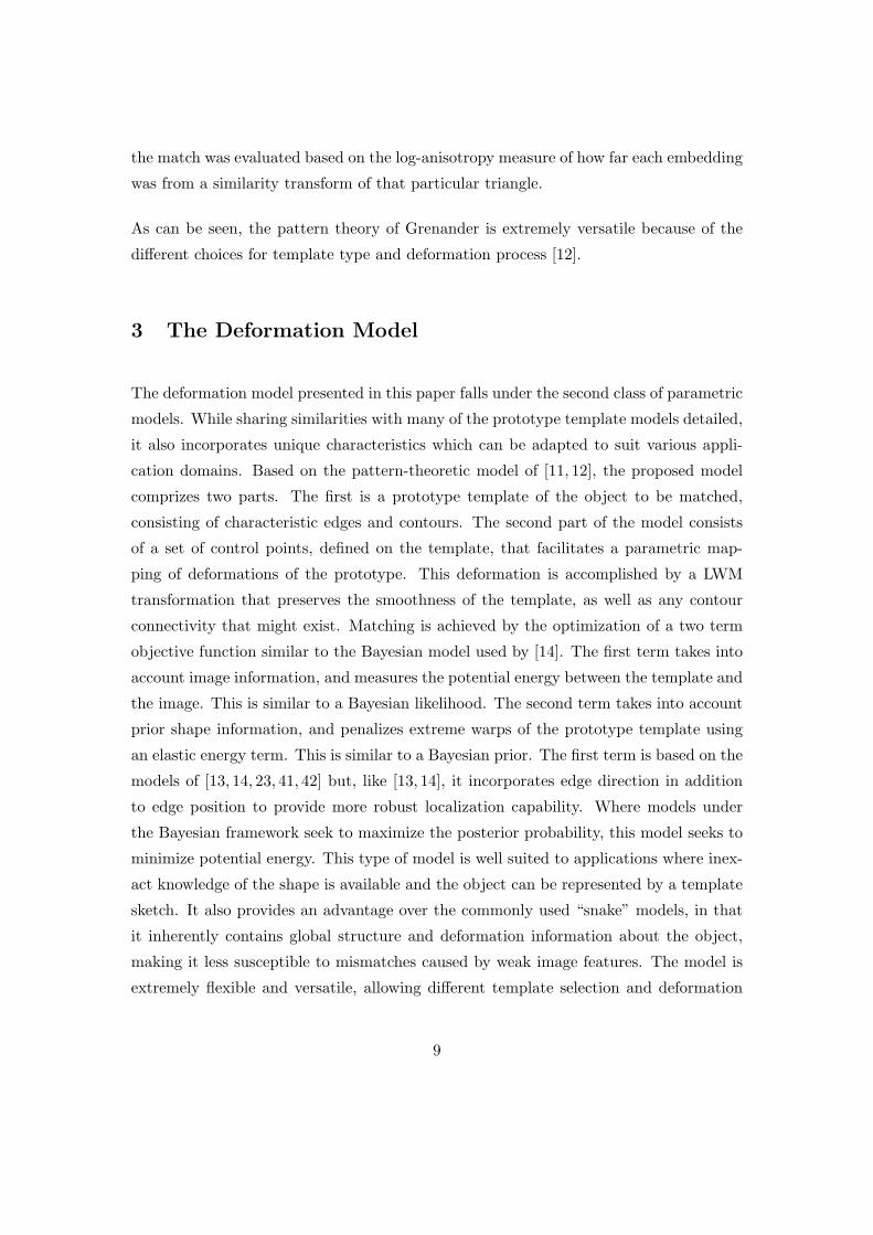
controls to be applied in different application domains. Figure 1 gives an example of a
typical template sketch, with control points, along with an image containing the object
to be localized.
(a) (b)
Figure 1: Deformable template model: (a) A prototype template of a Clownfish, with
control points shown. (b) An image containing a Clownfish to be localized.
The definition for shape given in [43] states that: “Shape is all the geometrical infor-
mation that remains when location, scale and rotational effects are filtered out from an
object.” It is therefore required that an object localization scheme, based on shape, be
invariant to changes in translation, scale and orientation, as well as acceptable deforma-
tions of the object [44]. Invariance to these characteristics is accomplished by utilizing
specific, discrete template instances and orientations at each stage of the algorithm.
Although effective, the requirement to test several discrete instances increases computa-
tional complexity, and is considered the main disadvantage with all template matching
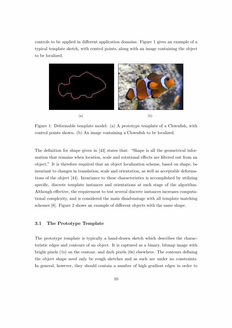
schemes [8]. Figure 2 shows an example of different objects with the same shape.
3.1 The Prototype Template
The prototype template is typically a hand-drawn sketch which describes the charac-
teristic edges and contours of an object. It is captured as a binary, bitmap image with
bright pixels (1s) on the contour, and dark pixels (0s) elsewhere. The contours defining
the object shape need only be rough sketches and as such are under no constraints.
In general, however, they should contain a number of high gradient edges in order to
10
Figure 2: Defining shape: Different instances of objects with the same shape.
represent only similarly shaped objects in an image [44]. Contours do not necessarily
need to be closed or connected, and they may be comprized of several components. This
flexibility allows the template to represent both the boundary and internal structure of
the object. This template scheme captures the global structure of an object without
requiring or specifying a parametric form for each shape class. It allows the embedding
of a priori knowledge of object shape within an intuitive framework and has the further
advantage that the amount of data is reduced significantly while retaining most of the
image information. The inherent structure captured by the deformable template im-
proves the algorithm’s robustness in the incidence of weak, occluded or missing image
features.
3.2 Control Points
The prototype template describes only a single, although most likely, instance of the
object. In order to match similar objects in an image, a set of deformed templates is re-
quired. Therefore, in addition to the template sketch, the deformation model is specified
along with a set of control points to be used for image warping. These control points,
placed at desired coordinates on the template, act as anchors for a LWM transformation
that can be applied to the prototype template to obtain deformations of the typical
shape.
11
Control points in image registration applications are placed at distinct locations on the
images. In [14], the authors used radial basis functions arranged in a grid pattern to
facilitate image warping. LWM warping has the advantage that control points can be
placed anywhere on the template. As such, expert knowledge of deformation can be
incorporated into the model by placing control points to specifically aid the expected
type of deformation. Landmarks such as vertices, midpoints, centroids and centers of
mass are typical of expert knowledge [45], but LWM warping can also utilize control
points placed in a grid pattern, or even at random. If control points are placed on
the actual contour, the warp can be thought of as a bending of the contour at those
specific points, whereas if the control points are placed randomly, or in a grid pattern,
the warping can be visualised as the stretching of a 2D surface such as a rubber mat.
Templates (edges and control points) may be obtained from training samples [46] or, as
in this case, constructed from high-level, expert knowledge.
4 The Multistage Algorithm
One major problem of object localization algorithms is that of search space size. In
typical applications, an object has to be retrieved regardless of translation, rotation and
size. Given that the localization also needs to be invariant to partial shape changes in
the target, this introduces a large number of variables to be determined during optimiza-
tion. Objective functions of the type found in localization applications are typically not
unimodal, and require a significant reduction of search space size in order to be computa-
tionally tractable [14]. A popular method used to accomplish the required search space
reduction is to use a multiresolution algorithm. The algorithm presented in this paper
takes the multiresolution approach one step further: it uses a multistage algorithm to
reduce the search complexity by first reducing the physical size of the search space, and
then iteratively reducing the number of variables to be optimized at each resolution.
The first stage of the algorithm is designed to reduce the physical size of the search
space, the second stage to reduce the number of variables by determining likely values for
template rotation, scale, and translation, and the third stage to determine the required
warp deformation for the template. Although described separately, stages two and three
12
form the multiresolution segment of the algorithm and are performed repeatedly, one
after the other, with an increase in resolution at each repetition.
4.1 Stage One - Regions of Interest
In the first stage of the algorithm, the physical size of the search space is reduced by
identifying regions in the image likely to provide a template match. This is accomplished
using cross-correlation, a standard approach to feature detection. Cross-correlation be-
tween two images can be defined as a comparison of the two image signals at all possible
relative positions [47]. It is used to measure the similarity between the template and the
region of the image with which it is aligned. The image is essentially filtered with the
template by convolving the two together and identifying regions where the overlapping
template and image window share similar values.
The similarity between the template (T) and the base image (I) is evaluated by measuring
the sum of the square of the differences between values in the template and the image.
The sum of the squared Euclidean distance is given by [48]:
d2T,I(u, v) =
N∑x,y
[T (x, y)− I(x− u, y − v)]2 (1)
Where the sum is taken over x, y for the N pixels of the template window positioned
over the image at u, v. Equation 1 can be expanded to:
d2T,I(u, v) =
N∑x,y
[T 2(x, y)− 2T (x, y)I(x− u, y − v) + I2(x− u, y − v)]
or:
d2T,I(u, v) =
N∑x,y
T 2(x, y) +N∑x,y
I2(x− u, y − v)− 2N∑x,y
T (x, y)I(x− u, y − v)
It can now be seen that the term∑
T 2(x, y) depends only on the template, and will
be constant for every pixel in the image. The second term,∑
I2(x− u, y − v), is the
sum of the square of the pixel values in the image that overlap the template. In images
where the target object is well segmented from the background clutter, this remains
13
approximately constant for poorly matching regions [49]. The remaining term is twice
the negative value of the correlation between T and I, and will increase as the Euclidean
distance between them decreases. This yields the cross-correlation term which is used to
measure the similarity between the template and the image window. It is given by [50]:
c(u, v) =N∑x,y
T (x, y)I(x− u, y − v) (2)
This provides an intuitive method for using correlation to match a template to an image,
since places where the correlation is high tend to be locations where the template and
image match well.
Correlation provides simplicity in that it is shift invariant, meaning that the operation
is unchanging for every pixel, and in that it is linear, replacing every pixel with a linear
combination of its neighbors [50]. There are, however, a number of disadvantages to
using (2) for template matching [49]:
• The range of c(u, v) is dependent on the size of the template.
• c(u, v) is susceptible to changes in amplitude such as those caused by varying light
conditions.
• In images where the target is not clearly segmented from a cluttered background,
the image energy term,∑
I2(x− u, y − v), may vary with position. This may
cause matching to fail, since high intensity regions may cause spurious correlation.
These problems can be overcome by normalising the template and image window vectors
to unit length. This yields a cosine-like correlation coefficient, known as the normalised
cross-correlation (NCC), given by [49]:
γ(u, v) =
∑Nx,y[T (x, y)− T ][I(x− u, y − v)− Iu,v]{∑N
x,y[T (x, y)− T ]2∑N
x,y[I(x− u, y − v)− Iu,v]2} 1
2
(3)
Where T is the mean of the template and Iu,v is the mean of the image under the
template window.
14
The peaks of the cross-correlation matrix occur where the template and image are best
correlated. The NCC can be displayed as a surface plot or as an intensity image, the
maxima of which are used to identify areas in the image where localization is likely
to occur. The NCC is thresholded and dilated to isolate these areas, which are then
transformed into a binary image mask. The mask overlaid on the image defines the
regions of interest, forming the output of this stage of the algorithm.
NCC is not an ideal approach to feature matching, since it is not invariant with respect
to scale, rotation, and deformation. However, these properties are overcome at least
to some extent during this stage of the algorithm. Rotation invariance is achieved by
calculating the NCC for a number of templates at discrete rotations. Moderate scale
changes and deformations are accommodated by using an image’s EPF 1, as opposed
to the original image, as the I during NCC. The EPF “blurs” the edges of an image,
essentially allowing for more relaxed matching requirements, while still maintaining ro-
bustness against spurious correlations. This is critical to the algorithm’s ability to locate
objects with significant in-class shape variability. Stage one of the algorithm is graphi-
cally illustrated in Figure 3. This example finds the regions of interest for localizing an
eye in an image of a face.
4.2 Stage Two - Multiresolution Matching
The second stage of the algorithm is tasked with finding approximate matches between
the template and the structures within the image. This stage of the algorithm is based on
the principle of sequential similarity detection [51], which dictates that full precision is
needed only at the peaks of the correlation function, while reduced precision can be used
elsewhere. Template matching is accomplished by use of a modified Chamfer matching
technique [52].
Chamfer matching is an edge matching method, first proposed by Barrow et al [53],
that attempts to find the best fit for edge points from two images by minimizing a
generalized distance between them [44]. In a hierarchical Chamfer scheme, the matching
is performed not only in the original image resolution, but in a series of images, where1EPFs are detailed in the next section
15
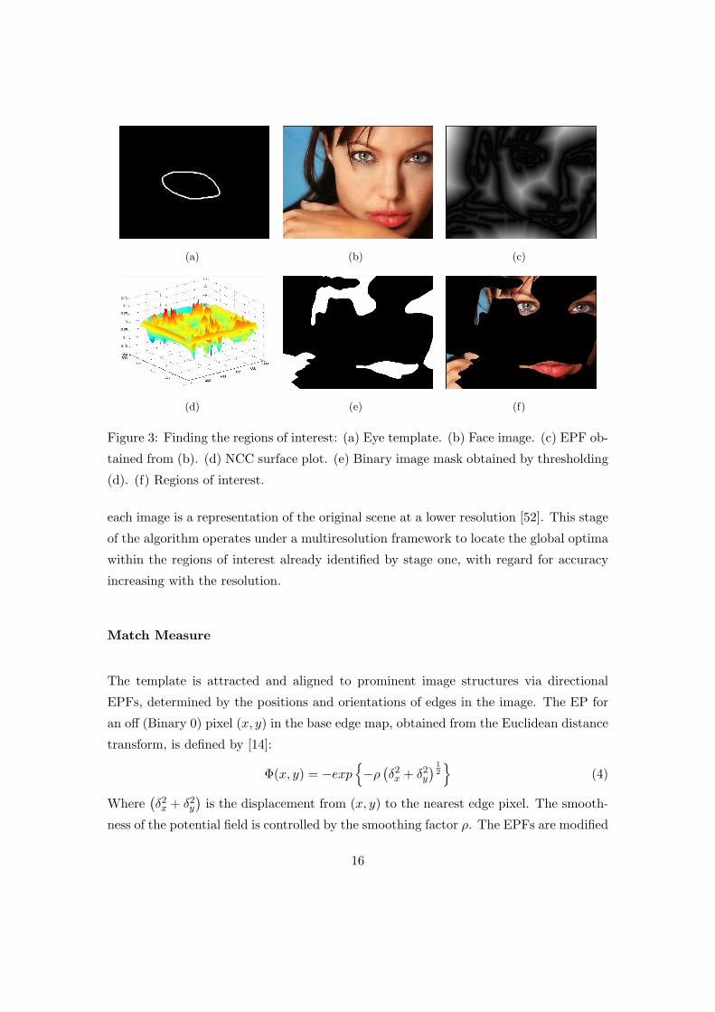
(a) (b) (c)
(d) (e) (f)
Figure 3: Finding the regions of interest: (a) Eye template. (b) Face image. (c) EPF ob-
tained from (b). (d) NCC surface plot. (e) Binary image mask obtained by thresholding
(d). (f) Regions of interest.
each image is a representation of the original scene at a lower resolution [52]. This stage
of the algorithm operates under a multiresolution framework to locate the global optima
within the regions of interest already identified by stage one, with regard for accuracy
increasing with the resolution.
Match Measure
The template is attracted and aligned to prominent image structures via directional
EPFs, determined by the positions and orientations of edges in the image. The EP for
an off (Binary 0) pixel (x, y) in the base edge map, obtained from the Euclidean distance
transform, is defined by [14]:
Φ(x, y) = −exp{−ρ
(δ2x + δ2
y
) 12
}(4)
Where(δ2x + δ2
y
)is the displacement from (x, y) to the nearest edge pixel. The smooth-
ness of the potential field is controlled by the smoothing factor ρ. The EPFs are modified
16
to include a directional component for each pixel (x, y) in edge K by [54]:
θ(x, y) = arctan
(∂K(x, y)
∂y/∂K(x, y)
∂x
)(5)
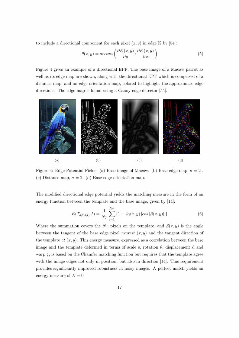
Figure 4 gives an example of a directional EPF. The base image of a Macaw parrot as
well as its edge map are shown, along with the directional EPF which is comprized of a
distance map, and an edge orientation map, colored to highlight the approximate edge
directions. The edge map is found using a Canny edge detector [55].
(a) (b) (c) (d)
Figure 4: Edge Potential Fields: (a) Base image of Macaw. (b) Base edge map, σ = 2 .
(c) Distance map, σ = 2. (d) Base edge orientation map.
The modified directional edge potential yields the matching measure in the form of an
energy function between the template and the base image, given by [14]:
E(Ts,θ,d,ζ , I) =1
NT
NT∑i=1
{1 + Φi(x, y) |cos [β(x, y)]|} (6)
Where the summation covers the NT pixels on the template, and β(x, y) is the angle
between the tangent of the base edge pixel nearest (x, y) and the tangent direction of
the template at (x, y). This energy measure, expressed as a correlation between the base
image and the template deformed in terms of scale s, rotation θ, displacement d and
warp ζ, is based on the Chamfer matching function but requires that the template agree
with the image edges not only in position, but also in direction [14]. This requirement
provides significantly improved robustness in noisy images. A perfect match yields an
energy measure of E = 0.
17
High energy template matches are immediately discarded, while low energy templates
(below an application-specific threshold) identified at this stage are now warped by stage
three of the algorithm to fit the image features more accurately. After the warp, the
energy function is re-evaluated and the warped templates are used as starting templates
for progressively finer resolutions.
Search Technique
The search for template matches is conducted by first finding approximate matches
at the coarsest resolution, with little regard for matching accuracy, and then using
these to initialize the search at progressively finer resolutions. At each resolution, the
search is conducted by windowing a set of discrete template instances and orientations
over the regions of interest in the image EPF and evaluating the match between them.
Only templates with energy below an application-specific threshold are examined at
increasing resolutions. Invariance to translation, rotation and scale is accomplished
at this stage of the algorithm by using varied sets of discrete template instances and
orientations at each resolution, with smaller step sizes between the discretizations at
higher resolutions. Although often application dependent, typical discretizations as well
as the match threshold required at each resolution are compared below.
Coarse Resolution:
Using the initial template Ti.
• Rotation: Templates are discretized to 12 orientations at 30◦ increments to span
the range [0◦; 360◦].
• Translation: These discretizations vary depending on the ratio of the template
size to the image size, ST : SI . Typical windowing step size could be 14ST .
• Scale: Templates are discretized to 3 sizes. As percentages of the initial template
size, these are 70%Ti, 100%Ti, 130%Ti.
• Match Threshold: Thresholds may vary depending on image types and appli-
cations. A typical threshold at this resolution would be E = 0.3.
18
Medium Resolution:
Using final template instances Tc, obtained from the coarse resolution warp.
• Rotation: Templates are discretized to 3 orientations of 15◦ increments to span
the range [θ(Tc)− 15◦; θ(Tc) + 15◦].
• Translation: Typical windowing step size could be 18ST .
• Scale: Templates are discretized to 3 sizes. As percentatges of the coarse template
size Tc, these are 90%Tc, 100%Tc, 110%Tc.
• Match Threshold: A typical threshold would be E = 0.2.
Fine Resolution:
Using final template instances Tm, obtained from the medium resolution warp.
• Rotation: Templates are discretized to 3 orientations at 5◦ increments to span
the range [θ(Tm) − 5◦; θ(Tm) + 5◦]. Any rotation within this range is expected to
be recovered by template deformation.
• Translation: Typical windowing step size could be 116ST .
• Scale: Template scales are not adjusted during this stage. Scale changes at this
resolution are expected to be recovered by template deformation.
• Match Threshold: A typical threshold would be E = 0.1.
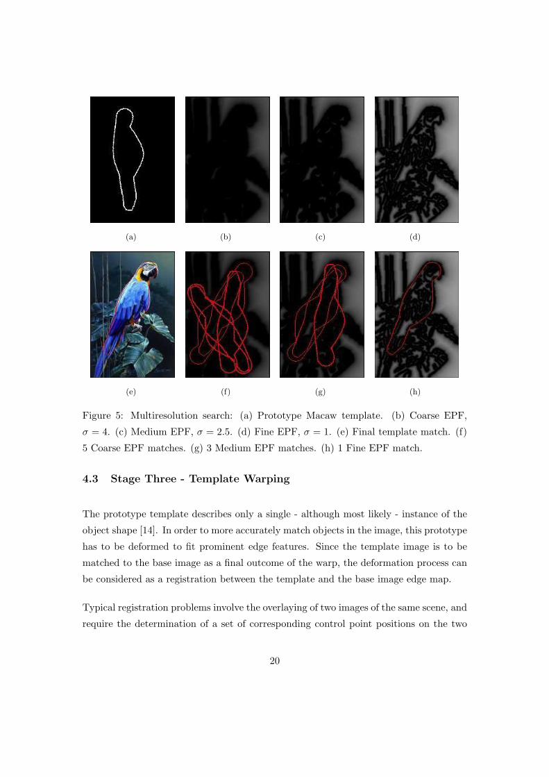
The multiresolution search is graphically illustrated in Figure 5. This example localizes
the Macaw in Figure 4 using the prototype template shown. The coarse, medium and fine
resolution EPFs are displayed along with the final template match and the approximate
matches at each resolution from the intermediate search stages. The EPFs are obtained
from the image edge maps, and their resolution is controlled by adjusting the standard
deviation σ of the Gaussian filter used in the Canny edge detector. No warping of
the template has been performed, and the displayed EPFs have undergone histogram
equalization to enhance their clarity for the benefit of the reader.
19
(a) (b) (c) (d)
(e) (f) (g) (h)
Figure 5: Multiresolution search: (a) Prototype Macaw template. (b) Coarse EPF,
σ = 4. (c) Medium EPF, σ = 2.5. (d) Fine EPF, σ = 1. (e) Final template match. (f)
5 Coarse EPF matches. (g) 3 Medium EPF matches. (h) 1 Fine EPF match.
4.3 Stage Three - Template Warping
The prototype template describes only a single - although most likely - instance of the
object shape [14]. In order to more accurately match objects in the image, this prototype
has to be deformed to fit prominent edge features. Since the template image is to be
matched to the base image as a final outcome of the warp, the deformation process can
be considered as a registration between the template and the base image edge map.
Typical registration problems involve the overlaying of two images of the same scene, and
require the determination of a set of corresponding control point positions on the two
20
images [45]. Once a correspondence between these control points has been established,
they are used to determine a transformation function that maps the rest of the points in
the image. Control point selection can be accomplished either manually or automatically.
Manual selection may require high level, expert knowledge, while automatic methods
typically rely on line intersections, locally maximum variances and curvatures or centers
of gravity as control point positions. Control point placement for the warp used in
this algorithm relies on a different approach, since the required control point locations
on the base image are unknown. The previous two stages of the algorithm have been
tasked with finding the regions of the global minima for localization, and the template
locations identified in stage two are used as starting positions for this stage. As such,
the templates are already partially aligned with the objects in the image and it can
be assumed that a control point on the base image will be in approximately the same
region as its corresponding control point on the template. Using this correspondence,
the alignment between the template and the image can be refined, and the templates can
be deformed to more accurately fit the image edges. The template warp ζ , along with
the stage two discretizations of rotation θ, scale s and translation d, yield deformations
of the prototype template T0 which are matched to the image using equation 6. The
deformed templates are of the form [14]:
Ts,θ,d,ζ(x, y) = T0 {s · [(x, y) + ζ (Rθ(x, y))] + (dx, dy)} (7)
Particle Swarm Optimization
Particle Swarm Optimization, developed in 1995 by Dr Russel Eberhart and Dr James
Kennedy, is a stochastic, population-based optimization method inspired by the social
behaviour of flocking birds and schooling fish [56]. It is an evolutionary technique in
which potential objective function solutions are modeled as particles in a swarm. These
particles (also known as individuals) “fly” through the problem space following the
current optimum particle [57]. During flight, each particle adjusts its trajectory towards
the optimum, according to both its own experience and the experiences of its neighboring
particles, making use of the best position encountered by itself and its neighbors. In this
way, the whole swarm contributes to the solution of the problem [57]. The use of Particle
Swarm optimization to determine control point placement is discussed here.
21
With the template overlaying the base image, the control point locations on the template
are used to approximate sets of corresponding control points on the base edge map. These
sets represent the individuals in the particle swarm. At each iteration of the swarm
optimization, the control points within the sets are shifted and the template is warped
to fit each set. This warp facilitates a registration between the deformed template and
the base image. The accuracy of the registration is determined by once again measuring
the energy between the now deformed template, and the base image edge map. The
optimization can be run for a set number of iterations, or until some termination criteria,
such as a minimum energy, is met. The Particle Swarm Optimization algorithm, its
implementation and its application to control point placement, is detailed extensively
in [58].
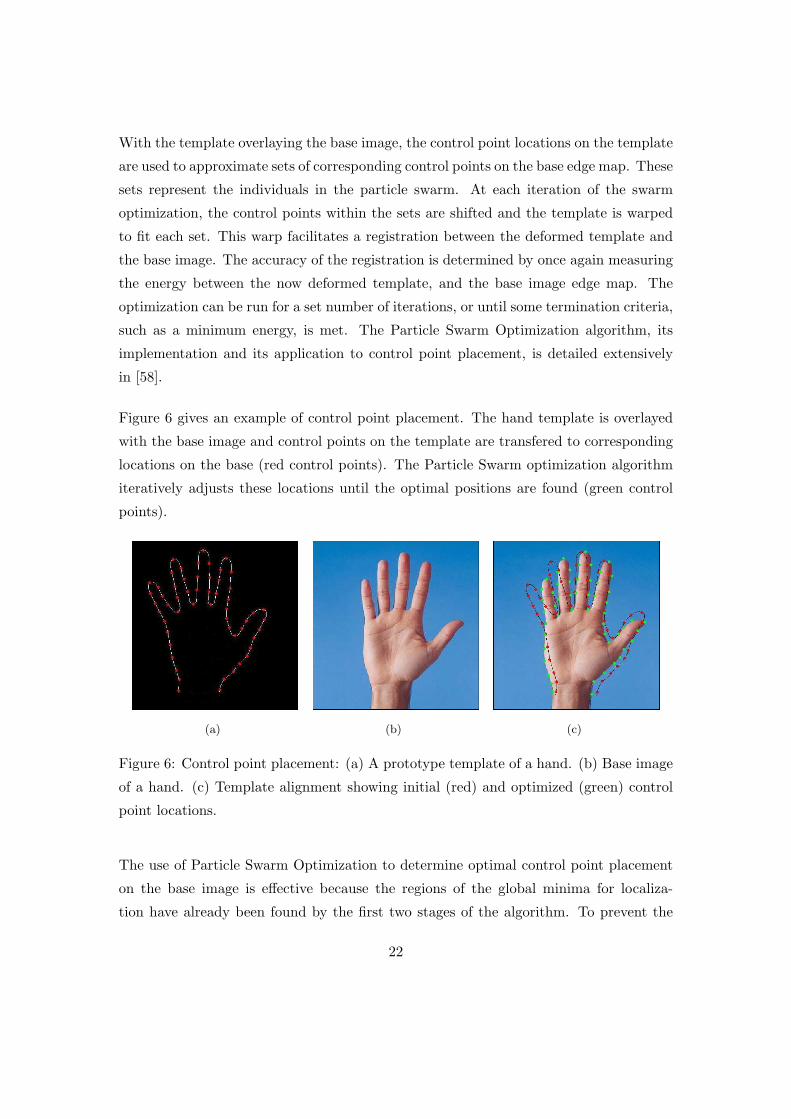
Figure 6 gives an example of control point placement. The hand template is overlayed
with the base image and control points on the template are transfered to corresponding
locations on the base (red control points). The Particle Swarm optimization algorithm
iteratively adjusts these locations until the optimal positions are found (green control
points).
(a) (b) (c)
Figure 6: Control point placement: (a) A prototype template of a hand. (b) Base image
of a hand. (c) Template alignment showing initial (red) and optimized (green) control
point locations.
The use of Particle Swarm Optimization to determine optimal control point placement
on the base image is effective because the regions of the global minima for localiza-
tion have already been found by the first two stages of the algorithm. To prevent the
22
swarm from exploring outside these regions, as well as to limit warp dimensionality,
a penalty function is introduced that penalizes extreme warps that would deform the
template to impractical shapes. This function penalizes the Euclidean distance between
corresponding control points on the template and base images, and ensures that during
optimization, the swarm does not move the control points inordinate distances. The
penalty function is added to the energy measure of equation 6. It is given by equation 8,
where α controls the rigidity of the warp. The initial α is inversely proportional to the
base image diagonal length, and is adjusted to reflect the expected variations in object
shape. An increased α is applied to rigid object structures and decreased α to flexible
ones.
P (x, y) = αN∑
i=1
{(xi −Xi)2 + (yi − Yi)
} 12 (8)
Defining a Warp Transformation Function
Inference of the appropriate transformation function is crucial to the accuracy of regis-
tration. Global transformations are typically used to register images that do not contain
local geometric distortion [45]; however, template registration may require local geo-
metric distortion depending on the local structure of the scene. The locally sensitive
transformation function used for template warping in this algorithm is described here.
Given N corresponding control points (Xi, Yi) on the template and (xi, yi) on the base
image, the LWM warp requires two functions, Xi ≈ f(xi, yi) and Yi ≈ g(xi, yi), that
approximate a mapping between these points as accurately as possible [45]. The problem
is reformulated to give two sets of N 3D points, (xi, yi, Xi) and (xi, yi, Yi), requiring the
determination of the functions f and g [45]. The determination of the function f only
is described here, since the function g can be determined in the same manner.
Given the set of N control points (xi, yi, Xi), a transformation function is required such
that when the coordinates of a control point on the base image are applied to it, it will
approximate the X-component of the corresponding control point on the template. f is
23
typically taken to be a polynomial of order M , of the form [45,59]:
f(x, y) =M∑
j=0
j∑k=0
ajkxkyj−k (9)
The parameters ajk of the polynomial can be determined using the least-squares method
to minimize the error:
E =N∑
i=1
[f(xi, yi)−Xi]2 (10)
Since this equation is a function of the parameters ajk, its solution requires the determi-
nation of the partial derivatives of E with respect to each parameter. Solving for each
partial derivative set equal to zero yields the system of linear equations known as the
normal equations [60]:M∑
j=0
j∑k=0
ajk
[N∑
i=1
xliy
m−1i xk
i yj−ki
]=
N∑i=1
Xixliy
m−li
l = 0, . . . ,M ; m = 0, . . . , l. (11)
Incorporating Orthogonal Polynomials
The system described above consists of T = (M + 2)(M + 1)/2 linear equations and is
solvable provided N ≥ T ; however, as T increases, the system becomes unstable and
inaccurate. To avoid this, a set of N polynomials are constructed by the Gramm-Schmidt
orthogonalization process, using a set of linearly independent functions, hi(x, y), to have
the form [61]:
P0(x, y) = a00h0(x, y)
P1(x, y) = a10P0(x, y) + a11h1(x, y)
P2(x, y) = a20P0(x, y) + a21P1(x, y) + a22h2(x, y)...
PT (x, y) = aT0P0(x, y) + aT1P1(x, y) + . . . + aTT hT (x, y) (12)
Determination of parameters ajk can now be accomplished by fixing values of aj0 and
applying the following orthogonalization property to the polynomials [62]:N∑
i=1
Pk(xi, yi)Pl(xi, yi) = 0 k 6= 1. (13)
24
If aj0 = 1 is assumed for all values of j, then the parameters of the polynomials can be
found using [62]:
ajj = −∑N
i=1[P0(xi, yi)]2∑Ni=1 P0(xi, yi)hj(xi, yi)
j = 1, . . . , T.
ajk = −ajj
∑Ni=1 Pk(xi, yi)hj(xi, yi)∑N
i=1[Pk(xi, yi)]2
j = 1, . . . , T ; k = 1, . . . , T − 1. (14)
Using a combination of orthogonal polynomials yields a transformation function [45]:
f(x, y) =T∑
j=0
ajPj(x, y) (15)
By substituting this new function into equation 10, once again solving for each par-
tial derivative set equal to zero, and again applying the orthogonalization property of
equation 13, it can be shown that the coefficients aj can be found using [45]:
aj =∑N
i=1 XiPj(xi, yi)∑Ni=1[Pj(xi, yi)]2
(16)
As can be seen, if orthogonal polynomials are used, the solution of the system of equations
is not required to determine the parameters of f . Another advantage of using orthogonal
polynomials is that if the required accuracy of the transformation function changes, the
required additional polynomials can simply be added to the system, without the need
to recompute the old ones [45].
Accounting for Local Geometric Difference
A disadvantage with using the least-squares method of error determination is that lo-
cal geometric differences, as well as local control point inaccuracies, are averaged out
equally over the whole image [45]. The effect of geometric difference and/or measure-
ment inaccuracy is the same irrespective of how near or far the control point is to the
approximating point. This is a highly undesirable property for a template warp that
25
requires local geometric distortion to achieve the required deformation. To localize the
least-squares method, a weight function is defined that represents the influence of each
ith control on a point (x, y) by the inverse Euclidean distance between them. The weight
function is give by [63]:
Wi(x, y) = [δ + (x− xi)2 + (y − yi)2]−12 (17)
Where δ defines the influence of control points on the approximating point. The smaller
the value of δ the smaller the influence of distant control points, allowing a more local
warp. Large values of δ decrease the influence of nearby control points, allowing for a
smoother warp. δ also prevents the weight function from becoming infinite where x = xi
and y = yi. As can be seen, different weights Wi(x, y) are obtained for different points
(x, y) and can therefore be considered as a function of the position of points in the base
image. By incorporating the weighting factor into the set of polynomials of equation 12
and again applying the orthogonalization property of equation 13, the parameters can
be shown, through an adaptation of equation 14, to be given by [62]:
ajj(x, y) = −∑N
i=1 Wi(x, y)[P0(xi, yi)]2∑Ni=1 Wi(x, y)P0(xi, yi)hj(xi, yi)
j = 1, . . . , T.
ajk(x, y) = −ajj(x, y)∑N
i=1 Wi(x, y)Pk(xi, yi)hj(xi, yi)∑Ni=1 Wi(x, y)[Pk(xi, yi)]2
j = 1, . . . , T ; k = 1, . . . , T − 1. (18)
Since the approximating transformation is still defined by equation 15, similarly to equa-
tion 16, the new coefficients aj can be found using [45]:
aj(x, y) =∑N
i=1 Wi(x, y)XiPj(xi, yi)∑Ni=1[Wi(x, y)Pj(xi, yi)]2
(19)
Local Weighted Mean Warp
Consider a point (x, y) in the base image, near to control point i. It is expected that
the corresponding point on the template is also near to control point i. Therefore it
26
can be assumed that the X value of a point (x, y) may be determined by the X values
of the nearby control points, according to an appropriate weighting function [45]. The
transformation function, known as the weighted mean, is defined to have the form [64]:
f(x, y) =∑N
i=1 Wi(x, y)Xi∑Ni=1 Wi(x, y)
(20)
Utilizing the weight definition of equation 17, this function generates a surface that
passes through the N 3D points (xi, yi, Xi) [64, 65]. The weighting function favours
measurements from near points over distant ones, but still uses the entire measurement
to determine the values of each point. This means that a local geometric distortion
influences the deformation of the entire template image. In order to obtain a strictly
local geometric warp, a transformation function is required that is influenced only by
the appropriate 3D point and n − 1 of its nearest neighbors [45]. This is accomplished
by adapting the weighting function to be [45]:{Wi(R) = 1− 3R2 + 2R3 0 ≤ R ≤ 1.
Wi(R) = 0 R ≥ 1.(21)
Where R = [δ + (x− xi)2 + (y − yi)2]12 /Rn and Rn is the distance of point (xi, yi) from
its (n− 1)th nearest control point in the base image. This guarantees that polynomial i
has no influence on points whose distance from control point (xi, yi) is larger than Rn.
The weighted sum of the polynomials is continuous and smooth at all values of (x, y),
since [45]:[
dWdR
]R=0
=[
dWdR
]R=1
= 0. This yields the final transformation function which
defines the X value (in the template) of an arbitrary point (x, y) (in the base image) by
the weighted sum of polynomials having a non-zero weight over that point. The Local
Weighted Mean function is given by [45,66]:
f(x, y) =
∑Ni=1 W
{[δ + (x− xi)2 + (y − yi)2]
12 /Rn
}Pi(x, y)∑N
i=1 W{
[δ + (x− xi)2 + (y − yi)2]12 /Rn
} (22)
Where Pi(x, y) is the polynomial passing through point (xi, yi, Xi) and n−1 other points
nearest to it.
LWM warping possesses a number of advantages over other warp methodologies [59]:
• Orthogonal Polynomials: As stated previously, the use of these allows for a
component of the transformation to be obtained directly from the corresponding
27
control points, obviating the need for the solution of a system of equations. More
polynomials can also be added as required, without the need to recompute the
existing ones.
• Approximate Transformation Functions: Since corresponding control points
are not mapped exactly to each other, digital errors in correspondence as well as
mismatch errors are automatically accounted for and smoothed by the warp.
• Adaptive Weight Functions: The rational weight functions adapt to the loca-
tions and densities of the control points. They automatically extend to sparcely
populated areas and increase or decrease in width according to the spacing be-
tween the points. This removes the stringent accuracy requirements typical of
control point selection, and makes it possible to warp templates where the density
of the points varies considerably in the image domain. The width of the weight
functions can also be globally controlled to vary the smoothness or rigidity of the
warp.
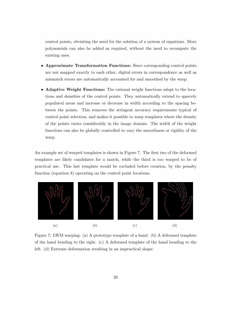
An example set of warped templates is shown in Figure 7. The first two of the deformed
templates are likely candidates for a match, while the third is too warped to be of
practical use. This last template would be excluded before creation, by the penalty
function (equation 8) operating on the control point locations.
(a) (b) (c) (d)
Figure 7: LWM warping: (a) A prototype template of a hand. (b) A deformed template
of the hand bending to the right. (c) A deformed template of the hand bending to the
left. (d) Extreme deformation resulting in an impractical shape.
28
5 Experimental Results
The localization algorithm presented in this paper has been applied to a variety of
different objects in several images. Results are given for a number of test applications
and have been divided into five categories, each illustrating a different aspect of, and
highlighting different capabilities of, the algorithm.
The experimental results presented here vary considerably with respect to a number of
important features. Background clutter in an image influences the effectiveness of the
cross-correlation results from stage one. Image and template sizes, as well as the ratio
of the template size to the image size ST : SI for each application define how long a
particular multiresolution search will take. The complexity of the required template warp
changes the iteration requirements for the Particle Swarm optimization and the LWM
warp. The code platform (MatlabTM in this case) also greatly affects computation time.
A comparative study of these factors is therefore not useful. The time per localization
varies between approximately 5s for low ST : SI and 40s for high.
With the exception of the section regarding scale invariance, all template images have
all been enlarged for clarity.
5.1 Search Capability
The first category of experiments illustrates the search capability of the algorithm, high-
lighting the translation invariance of the localization scheme. The multistage, multireso-
lution approach is used to automatically locate objects of interest within the given image.
A number of small (relative to the image size) objects of different shapes are localized
independently using different prototype templates. The algorithm is able to search a
complex image and successfully identify the required objects. The search capability of
the algorithm is highlighted in Figure 8.
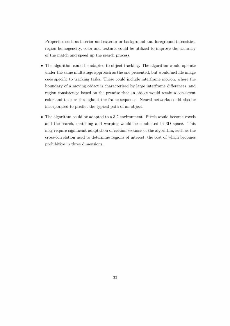
Figure 8a shows five independent templates for the letters G O L and F as well as
for the VW logo. These template structures are to be identified in Figure 8b. Figure
8c (and the magnification in Figure 8e) shows the localization results at the medium
29
resolution, showing the spurious localization of the vehicle’s front right lights and the
T in the licence plate (from the F template). However, at the fine resolution level of
Figure 8d (and the magnification in Figure 8f), the correct localization is achieved.
This experiment also illustrates two further properties of the algorithm. It shows that the
algorithm can localize complex shapes using multiply-connected templates with internal
structure (VW logo), and highlights the ability of the algorithm to identify text within
images. By noting which templates successfully localize letters (and at what locations),
text can effectively be read by the algorithm.
5.2 Template Convergence
The second category of experiments demonstrates the warp capability of the algorithm,
and shows how the templates are able to locally deform to match the objects in the
image. The template is initially overlayed on the coarse resolution image EPF , and
is shifted to obtain the best match. Particle Swarm optimization is then used to warp
the template to fit the object features before increasing the resolution and repeating the
process.
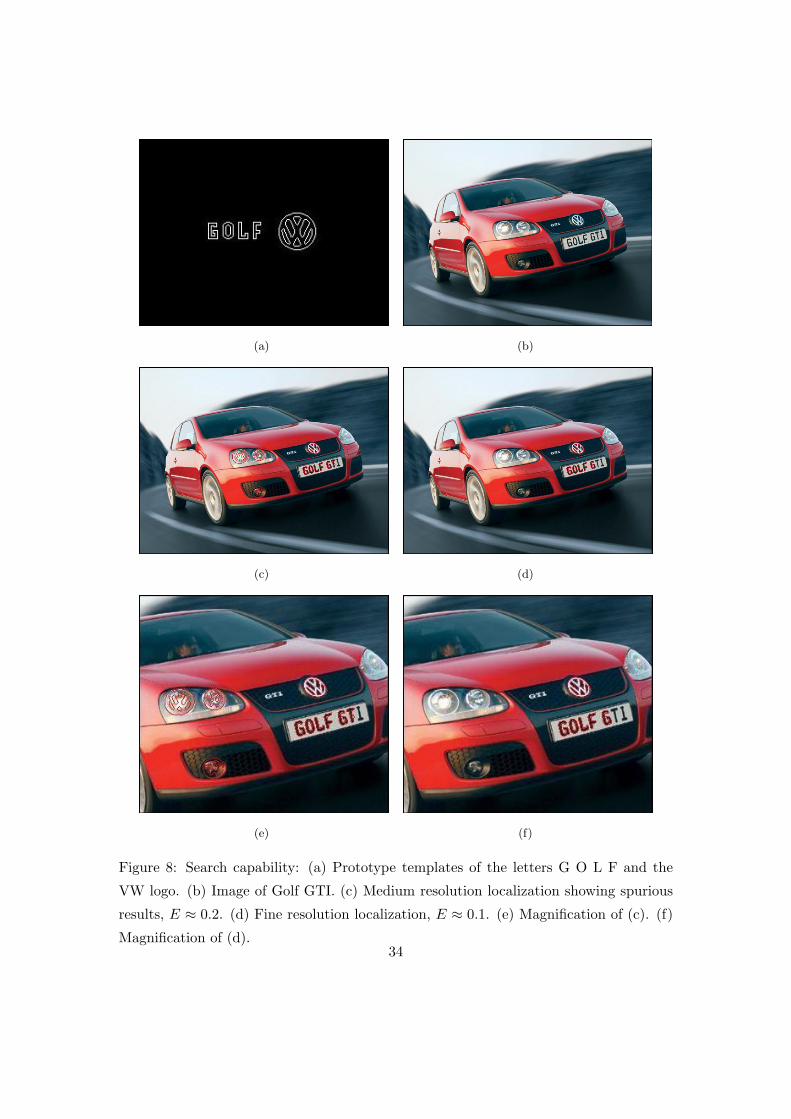
Figure 9 shows the deformation process for localizing a Snowy Owl. The prototype
template match as well as snapshots of the final deformed templates at each resolution are
presented to illustrate how the template evolves to match the salient object structures.
The object is correctly retrieved and template convergence toward the object contours
can be seen clearly.
5.3 Rotation Invariance
The aim of the third category of experiments is to demonstrate the rotation invariance
of the localization algorithm. This is accomplished by utilizing a set of discrete template
instances to find objects at different rotations.
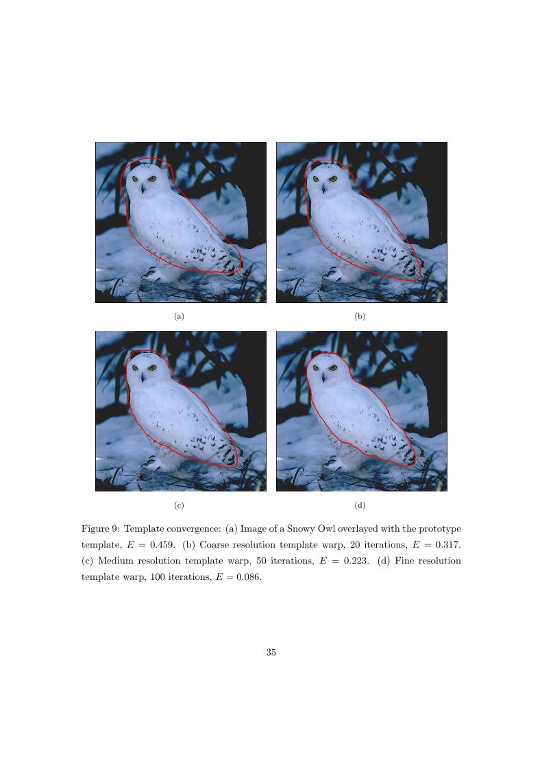
Figure 10 shows the localization of windmill blades at orientations around 360◦. To be
noted in the magnified image of Figure 10c, is the occurance of two spurious localizations
30
of windmill blades at the bottom of the windmill circle (approximately 260◦ and 280◦).
These are due to the edges of windmill base providing the required structure for localiza-
tion. Scale invariance was removed from the algorithm for this experiment by restricting
the template scale to the original size. This was done to exclude the localizations of the
windmill blade shape within the windmill strut.
This experiment also illustrates the algorithm’s ability to identify multiple instances
of the same object. Since this is an inherent property of the search technique, apart
from having to examine these additional matches more closely at each resolution, no
additional computational overhead is involved (this is not true of warping the template
to fit multiple objects).
5.4 Scale Invariance
Category four experimentation results illustrate the scale invariance of the localization
scheme. This is demonstrated by localizing multiple objects of similar shape but varying
scale, using a set of discrete template instances that are scaled versions of the original.
Figure 11 shows the localization of Arches in the Segovia Aqueduct, using the prototype
template shown. The original template is used to localize the arches at the top right
of the image, and a “slanted” affine warp of the original template is used to generate
templates for the narrower arches. The smaller arches in the center of the bottom row
are localized using 25% and 50% scaled versions of the original template. Multiple scaled
localizations are correctly retrieved in this manner.
5.5 Object Tracking
The fifth category of experiments highlights a consequential property of the localization
algorithm, that of object tracking.
The images in Figure 12 show four different hand images, each slightly different from the
next in terms of both shape and orientation. By first using the prototype template to
localize the hand in the first frame of Figure 12b, and then using the final template from
31
each image as the prototype template for the subsequent one, the hand can be tracked
through the four frames. The use of evolving prototype templates allows the algorithm
to accommodate the variations in shape of the hands in each image.
Although the inherent properties of the localization algorithm allow it to track simple
objects by performing a full localization on each frame, it is not as efficient or as effective
as dedicated template tracking schemes that use additional image cues such as region
consistency and interframe motion to reduce computational complexity [67]. This set of
experiments also illustrates the fact that the localization algorithm can handle prototype
templates that consist of open contours.
6 Conclusion and Future Work
An algorithm has been presented for the localization of objects in images using de-
formable templates. The deformable model consists of a hand-drawn, prototype tem-
plate intended to capture a priori knowledge about the object shape, as well as a set of
control points on the template. These points are used in a LWM warp to obtain deforma-
tions of the object shape. A multistage, multiresolution algorithm has been presented,
detailing the different stages used in the search and matching process. The algorithm
reduces computational complexity by first using cross-correlation to reduce the physical
size of the search space, and then reducing the number of variables to be optimized at
each stage using an adapted, hierarchical Chamfer matching scheme. Warping is ac-
complished as a registration between the template and the image, using Particle Swarm
optimization to locate the optimal control point locations. Test results for a number
of images have been given, with each set of results highlighting a different aspect, and
different capabilities, of the algorithm. The quality of the results is a consequence of the
combination of a search technique that can efficiently find a global optimal solution to
the non-rigid matching problem, and a warping method that inherently takes advantage
of the prior shape knowledge.
Future work in this field could proceed along, inter alia, the following lines:
• The algorithm could be adapted to include image attributes other than shape alone.
32
Properties such as interior and exterior or background and foreground intensities,
region homogeneity, color and texture, could be utilized to improve the accuracy
of the match and speed up the search process.
• The algorithm could be adapted to object tracking. The algorithm would operate
under the same multistage approach as the one presented, but would include image
cues specific to tracking tasks. These could include interframe motion, where the
boundary of a moving object is characterised by large interframe differences, and
region consistency, based on the premise that an object would retain a consistent
color and texture throughout the frame sequence. Neural networks could also be
incorporated to predict the typical path of an object.
• The algorithm could be adapted to a 3D environment. Pixels would become voxels
and the search, matching and warping would be conducted in 3D space. This
may require significant adaptation of certain sections of the algorithm, such as the
cross-correlation used to determine regions of interest, the cost of which becomes
prohibitive in three dimensions.
33
(a) (b)
(c) (d)
(e) (f)
Figure 8: Search capability: (a) Prototype templates of the letters G O L F and the
VW logo. (b) Image of Golf GTI. (c) Medium resolution localization showing spurious
results, E ≈ 0.2. (d) Fine resolution localization, E ≈ 0.1. (e) Magnification of (c). (f)
Magnification of (d).34
(a) (b)
(c) (d)
Figure 9: Template convergence: (a) Image of a Snowy Owl overlayed with the prototype
template, E = 0.459. (b) Coarse resolution template warp, 20 iterations, E = 0.317.
(c) Medium resolution template warp, 50 iterations, E = 0.223. (d) Fine resolution
template warp, 100 iterations, E = 0.086.
35
(a) (b)
(c) (d)
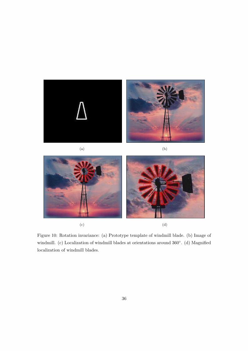
Figure 10: Rotation invariance: (a) Prototype template of windmill blade. (b) Image of
windmill. (c) Localization of windmill blades at orientations around 360◦. (d) Magnified
localization of windmill blades.
36
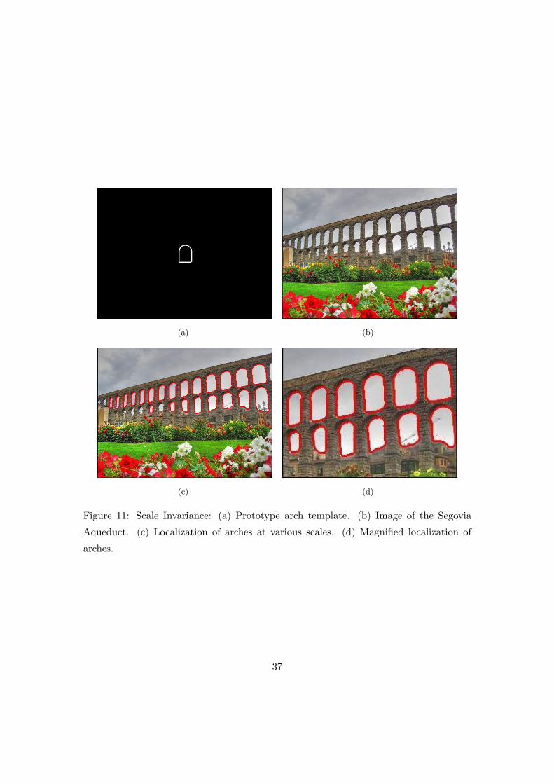
(a) (b)
(c) (d)
Figure 11: Scale Invariance: (a) Prototype arch template. (b) Image of the Segovia
Aqueduct. (c) Localization of arches at various scales. (d) Magnified localization of
arches.
37
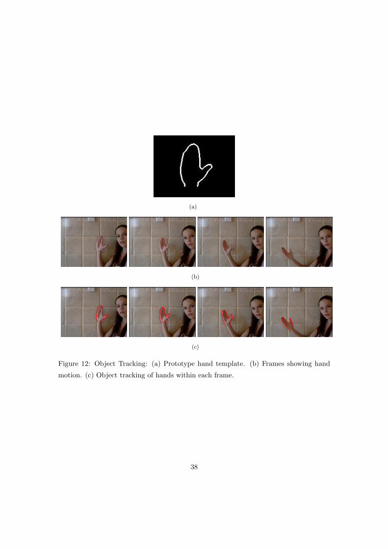
(a)
(b)
(c)
Figure 12: Object Tracking: (a) Prototype hand template. (b) Frames showing hand
motion. (c) Object tracking of hands within each frame.
38
References
[1] C. Faloutos, R. Barber, M. Flicker, J. Hafner, W. Niblack, and W. Equitz, “Effi-
cient and Effective Querying by Image Content,” Journal of Intelligent Information
Systems, vol. 3, no. 3, pp. 231–262, 1994.
[2] T. Kato, “Database Architecture for Content-Based Image Retrieval,” In Proceed-
ings of the SPIE - The International Society for Optical Engineering,, vol. 1662,
pp. 112–123, 1992.
[3] B. Holt and L. Hartwick, “Visual Image Retrieval for Applications in Art and Art
History,” Proc. SPIE, vol. 2185, pp. 70–81, February 1994.
[4] A. Yuille, “Deformable Templates for Face Recognition,” Journal of Cognitive Neu-
roscience, vol. 3, no. 1, pp. 59–70, 1991.
[5] M. P. Dubuisson-Jolly, S. Lakshmanan, and A. K. Jain, “Vehicle Segmentation and
Classification Using Deformable Templates,” PAMI, vol. 18, no. 3, pp. 293–308,
March 1996.
[6] D. Rueckert and P. Burger, “Geometrically Deformable Templates for Shape-Based
Segmentation and Tracking in Cardiac MR Image,” Proceedings of the International
Workshop on Energy Minimization Methods in Computer Vision and Pattern Recog-
nition, pp. 83–98, 1997.
[7] F. Poupon, J. F. Mangin, D. Hasboun, C. Poupon, I. Magnin, and V. Frouin,
“Multi-object Deformable Templates Dedicated to the Segmentation of Brain Deep
Structures,” in Proceedings of the First International Conference on Medical Image
39
Computing and Computer-Assisted Intervention (MICCAI ’98), M. Wells, Ed., vol.
LNCS, no. 1496. Berlin, Heidelberg: Springer-Verlag, 1998, pp. 1134–1143.
[8] E. Suarez, C. F. Westin, E. Rovaris, and J. Ruiz-Alzola, “Nonrigid Registration Us-
ing Regularized Matching Weighted by Local Structure,” in Proceedings of the Fifth
International Conference on Medical Image Computing and Computer-Assisted In-
tervention (MICCAI ’02), T. Dohi and R. Kikinis, Eds., vol. LNCS, no. 2489.
Berlin, Heidelberg: Springer-Verlag, 2002, pp. 581–589.
[9] S. K. Warfield, M. Kaus, F. A. Jolesz, and R. Kikinis, Medical Image Computing
and Computer-Assisted Intervention - MICCAI’98: First International Conference.
Springer Berlin / Heidelberg, W.M. Wells and A. Colchester and S. Delp, Eds.,
1996, vol. 1496, ch. Adaptive Template Moderated Spatially Varying Statistical
Classification, p. 431.
[10] P. Felzenszwalb, “Representation and Detection of Shapes in Images,” Ph.D. dis-
sertation, Massachusetts Institute of Technology, September 2003.
[11] U. Grenander, “Pattern Synthesis: Lectures in Pattern Theory,” Applied Mathe-
matical Sciences, vol. 18, Springer-Verlag, 1976.
[12] U. Grenander and D. M. Keenan, Towards Automated Image Understanding, Ad-
vances in Applied Statistics: Statistics and Images. Carfax Publishing Company,
1993, vol. 1, ch. 6, pp. 89–103.
[13] Y. Zhong, “Object Matching Using Deformable Templates,” PhD Thesis, Depart-
ment of Computer Science, Michigan State University, 1997.
[14] A. K. Jain, Y. Zhong, and S. Lakshmanan, “Object Matching Using Deformable
Templates,” IEEE Transactions on Pattern Analysis and Machine Intelligence,
vol. 18, no. 3, pp. 267–278, MARCH 1996.
[15] P. V. C. Hough, “Methods and Means for Recognising Complex Patterns,” U.S.
Patent 3069654, Tech. Rep., 1962.
[16] A. Rosenfeld, “Picture Processing by Computer: Survey,” Surveys, vol. 1, no. 3,
pp. 147–176, September 1969.
40
[17] D. H. Ballard, “Generalizing the Hough Transform to Detect Arbitrary Shapes,”
Pattern Recognition, vol. 13, pp. 111–122, 1981.
[18] D. H. Ballard and C. M. Brown, Computer Vision. Englewood Cliffs, NJ: Prentice-
Hall, 1982.
[19] J. Illingworth and J. Kitter, “A Survey of Hough Transform,” CVGIP, vol. 44, pp.
87–116, 1988.
[20] V. Leavers, “Survey: Which Hough transform?” CVGIP: Image Understanding,
vol. 58, pp. 250–264, 1993.
[21] D. J. Burr, “Elastic Matching of Line Drawings,” IEEE Transactions on Pattern
Analysis and Machine Intelligence, vol. 3, no. 2, pp. 708–713, November 1981.
[22] M. Moshfeghi, S. Ranganath, and K. Nawyn, “Three-Dimensional Eastic Matching
of Volumes,” IEEE Transactions on Pattern Analysis and Machine Intelligence,
vol. 3, no. 2, pp. 128–138, March 1994.
[23] M. Kass, A. Witkin, and D. Terzopoulos, “Snakes: Active Contour Models,” IJCV,
vol. 1, no. 4, pp. 321–331, 1988.
[24] D. Terzopoulos, A. Witkin, and M. Kass, “Constraints on Deformable Models:
Recovering 3D Shape and Nonrigid Motion,” AI, no. 36, pp. 91–123, 1988.
[25] L. Cohen and I. Cohen, “Finite-Element Methods for Active Contour Models and
Ballons for 2-D and 3-D Images,” IEEE Transactions on Pattern Analysis and
Machine Intelligence, vol. 15, no. 11, pp. 1131–1147, November 1993.
[26] T. F. Chan and L. A. Vese, “Active Contours Without Edges,” IEEE Transactions
on Image Processing, vol. 12, no. 2, pp. 266–277, February 2001.
[27] T. Kostiainen, I. Kalliomaeki, T. Tamminen, and J. Lampinen, “3D Object Recog-
nition Based on Hierarchical Eigen Shapes and Bayesian Inference,” in Proc. SPIE
Vol. 4572, p. 165-173, Intelligent Robots and Computer Vision XX: Algorithms,
Techniques, and Active Vision, D. P. Casasent and E. L. Hall, Eds., vol. 4572,
October 2001, pp. 165–173.
[28] J. Sullivan, A. Blake, M. Isard, and J. MacCormick, “Bayesian Object Localisation
in Images,” IJCV, vol. 44, no. 2, p. 111135, 2001.
41
[29] M. A. T. Figueiredo, J. M. N. Leito, and A. K. Jain, “Unsupervised Contour Rep-
resentation and Estimation Using B-Splines and a Minimum Description Length
Criterion,” IEEE Transactions on Image Processing, vol. 9, no. 6, pp. 1075–1087,
June 2001.
[30] F. Leymarie and M. D. Levine, “Tracking Deformable Objects in the Plane Using
an Active Contour Model,” IEEE Transactions on Pattern Analysis and Machine
Intelligence, vol. 15, no. 6, p. 617634, June 1993.
[31] A. Witkin, D. Terzopoulos, and M. Kass, “Signal Matching Through Scale Space,”
International Journal of Computer Vision, pp. 133–144, 1987.
[32] S. Lakshmanan and D. Grimmer, “A Deformable Template Approach to Detecting
Straight Edges in Radar Images,” IEEE Transactions on Pattern Analysis and
Machine Intelligence, vol. 18, no. 4, pp. 438–443, April 1996.
[33] A. L. Yuille, P. Hallinan, and D. Cohen, “Feature Extraction from Faces Using
Deformable Templates,” International Journal of Computer Vision, vol. 8, no. 2,
pp. 133–144, 1992.
[34] L. Staib and J. Duncan, “Boundary Finding with Parametrically Deformable Mod-
els,” IEEE Transactions on Pattern Analysis and Machine Intelligence, vol. 14,
no. 11, pp. 1061–1075, November 1992.
[35] A. Chakraborty, L. Staib, and J. Duncan, “Deformable Boundary Finding Influ-
enced by Region Homogeneity,” Proceedings of the IEEE conference on Computer
Vision and Pattern Recogntion, pp. 624–627, June 1994.
[36] M. A. Fischler and R. A. Elschlager, “The Representation and Matching of Pictorial
Structures,” IEEE Transactions on Computers, vol. 22, no. 1, pp. 67–92, 1973.
[37] B. Widrow, “The Rubber Mask Technique, Parts I and II,” Pattern Recognition,
vol. 5, pp. 175–211, 1973.
[38] U. Grenander, Y. Chow, and D. M. Keenan, Hands: a Pattern Theoretic Study of
Biological Shapes. New York, NY, USA: Springer-Verlag New York, Inc., 1991.
42
[39] Y. Amit, U. Grenander, and M. Piccioni, “Structural Image Restoration Through
Deformable Templates,” American Statistical Association Journal, vol. 86, no. 414,
pp. 376–387, 1991.
[40] T. Cootes, C. Taylor, and A. Lanitis, “Active Shape Models: Evaluation of a Mul-
tiresolution Method for Improving Image Searches,” Proceedings of the British Ma-
chine Vision Conference, vol. 1, pp. 327–336, 1994.
[41] M. A. T. Figueiredo and J. M. N. Leito, “Bayesian Estimation of Ventricular Con-
tours in Angiographic Images,” IEEE Transactions on Medical Imaging, vol. 11,
no. 11, pp. 416–429, September 1992.
[42] G. Storvik, “A Bayesian Approach to Dynamic Contours Through Stochastic Sam-
pling and Simulated Annealing,” IEEE Transactions on Pattern Analysis and Ma-
chine Intelligence, vol. 16, pp. 976–986, 1994.
[43] M. Leventon, W. Grimson, and O. Faugeras, “Statistical Shape Influence in Geo-
desic Active Contours,” IEEE Transactions on Computer Vision and Pattern Recog-
nition, vol. 1, pp. 316–323, 2000.
[44] L. Ding, A. Goshtasby, and M. Satter, “Volume Image Registration by Template
Matching,” Image and Vision Computing, vol. 19, no. 12, pp. 821–832, October
2001.
[45] A. Goshtasby, “Image Registration by Local Approximation Methods,” Image and
Vision Computing, vol. 6, no. 4, pp. 255–261, November 1988.
[46] C. K. I. Williams, M. Revow, and G. E. Hinton, “Instantiating Deformable Models
with a Neural Net,” Computer Vision and Image Understanding, vol. 68, no. 1, pp.
120–126, October 1997.
[47] A. Goshtasby, S. H. Gage, and J. F. Bartholic, “A Two-Stage Cross-Correlation
Approach to Template Matching,” IEEE Transactions on Pattern Analysis and
Machine Intelligence, vol. 6, no. 3, pp. 374–378, 1984.
[48] J. P. Lewis, “Fast Template Matching,” Vision Interface, pp. 120–123, 1995.
[49] J. Lewis, “Fast Normalized Cross-Correlation,” in Vision Interface. Canadian
Image Processing and Pattern Recognition Society, 1995, pp. 120–123.
43
[50] R. C. Gonzalez and P. Wintz, Digital Image Processing (3rd Edition), R. Woods,
Ed. Reading, Massachusetts: Addison-Wesley, 1992.
[51] D. I. Barnea and H. F. Silverman, “A Class of Algorithms for Fast Digital Image
Registration,” IEEE Transactions on Computers, vol. 21, pp. 179–186, 1972.
[52] G. Borgefors, “Hierarchical Chamfer Matching: A Parametric Edge Matching Algo-
rithm,” IEEE Transactions on Pattern Analysis and Machine Intelligence, vol. 10,
no. 6, pp. 849–865, November 1988.
[53] H. G. Barrow, J. M. Tenenbaum, R. C. Bolles, and H. C. Wolf, “Parametric Cor-
respondence and Chamfer Matching: Two New Techniques for Image Matching,”
Proceedings of the Fifth International Joint Conference on Artificial Intelligence,
pp. 659–663, 1977.
[54] M. Ulrich, C. Steger, and A. Baumgartner, “Real-Time Object Recognition Using
a Modified Generalized Hough Transform,” Pattern Recognition, vol. 36, pp. 2557–
2570, 2003.
[55] J. Canny, “A Computational Approach to Edge Detection,” IEEE Transactions on
Pattern Analysis and Machine Intelligence, vol. 8, no. 6, pp. 679–698, 1986.
[56] R. C. Eberhart, J. Kennedy, and Y. H. Shi., Swarm Intelligence. USA: Kauffman
Publishers, 2001.
[57] J. Kennedy and R. C. Eberhart, “Particle Swarm Optimization,” IEEE Interna-
tional Conference on Neural Networks, vol. 1, no. 1, 1995.
[58] J. Spiller and T. Marwala, “Evolutionary Algorithms for Warp Control Point Place-
ment,” March 2007, submitted to The 2nd International Symposium on Intelligence
Computation and Applications.
[59] L. Zagorchev and A. Goshtasby, “A Comparative Study of Transformation Func-
tions for Nonrigid Image Registration.” IEEE Transactions on Image Processing,
vol. 15, no. 3, pp. 529–538, March 2006.
[60] T. J. Rivlin, An Introduction to the Approximation of Functions. Waltham, MA,
USA: Blaisdell Publishing Co, 1969.
44
[61] H. F. Davis, Fourier Series and Orthogonal Functions. USA: Allyn and Bacon,
1966.
[62] G. E. Forsythe, “Generation and Use of Orthogonal Polynomials for Data Fitting
with a Digital Computer,” Journal of the Society of Industrial Applied Mathematics,
vol. 5, no. 2, pp. 74–88, 1957.
[63] D. H. McLain, Mathematical Methods in Computer Graphics Design, 1980, ch. In-
terpolation Methods for Erroneous Data, pp. 87–104.
[64] D. Shepard, “A Two-Dimensional Interpolation Function for Irregularly Spaced
Data,” Proceedings of the 23rd National Conference. ACM, pp. 517–524, 1968.
[65] I. K. Crain and B. K. Bhattacharyya, “Treatment of Non-Equispaced Two-
Dimensional Data with a Digital Computer,” Geoexploration, vol. 5, pp. 173–194,
1967.
[66] A. D. Maude, “Interpolation for Graph Plotters,” Journal of Computers, vol. 16,
pp. 64–65, 1973.
[67] Y. Zhong, A. K. Jain, and M. P. Dubuisson-Jolly, “Object Tracking Using De-
formable Templates,” IEEE Transactions on Pattern Analysis and Machine Intel-
ligence, vol. 22, no. 5, pp. 544–549, MAY 2000.
45
Chapter 2
Evolutionary Algorithms for Warp
Control Point Placement
This paper has been submitted to The 2nd International Symposium on Intelligence
Computation and Applications, to take place in Wuhan, China, during September 2007.
Accepted papers are to be published by Springer in LNCS. This paper deals with the
warp methodology of the localization algorithm, and presents a comparative analysis of
the evolutionary optimization methods tested for warp control point placement.
46
Evolutionary Algorithms for Warp Control PointPlacement
Jonathan Spiller and Tshilidzi Marwala
School of Electrical and Information Engineering,University of the Witwatersrand,
Johannesburg, South Africa{j.spiller,t.marwala}@ee.wits.ac.za
http://www.wits.ac.za
Abstract. Object localization requires the deformation and registrationof templates with a target image. A warping and registration methodol-ogy is presented to facilitate this task, utilizing evolutionary optimizationroutines to automatically determine optimal control point placement be-tween template and target image. The Local Weighted Mean warp usedto deform the templates to fit these control points is presented, alongwith a discussion of three evolutionary algorithms and their applicationto the problem. The optimization routines of Genetic Algorithm, ParticleSwarm Optimization and Simulated Annealing are compared in terms ofaccuracy, speed and computational requirements, with Particle SwarmOptimization being highlighted as the best method for this task.
Key words: Template Warping, Registration, Genetic Algorithm, Par-ticle Swarm Optimization, Simulated Annealing.
1 Introduction
Prototype-based localization schemes typically require the warping of templatesand their registration with a target image [1]. A general localization scheme ofthis type has been developed, that uses a multistage, multiresolution algorithmto facilitate a computationally efficient search. The initial stages of the algorithmare tasked with reducing the search space and determining approximate templatematches, while the final stage involves warping of the template to fit salient imagefeatures. A novel template warping and registration method, using evolutionaryalgorithms to determine optimal control point placement for template warping,has been developed specifically for this object localization algorithm. The aim ofthis research is to determine which of the evolutionary algorithms is best suitedfor use in the final algorithm implementation.
This paper presents the warp methodology of the localization algorithm,along with a comparison of the three evolutionary optimization techniques testedfor the determination of control point locations. These are:
– Genetic Algorithm (GA).
48 Evolutionary Algorithms for Warp Control Point Placement
– Particle Swarm Optimization (PSO).– Simulated Annealing (SA).
The template deformation method presented is adaptable to a wide vari-ety of warping and registration tasks [2], and the algorithm has already beensuccessfully applied to medical image segmentation [3], target recognition fromaerial images, text recognition, as well as general object localization tasks [2]. Acomprehensive review of the full localization algorithm is beyond the scope ofthis paper, but can be found in [2].
The rest of this paper is set out as follows: Section 2 gives a brief overviewof the registration problem, briefly discussing the algorithm and the registrationrequirements. Section 3 describes the warp methodology, detailing the LocalWeighted Mean warp. The thee evolutionary algorithms are detailed in Section 4.The results of a number of warp tests, as well as a comparison of the performancesof the three algorithms, are given in Section 5.
2 Registration for Object Localization
Typical registration problems involve the overlaying of two images of the samescene, and require the determination of a set of corresponding control pointpositions on the two images [4]. Once a correspondence between these controlpoints has been established, they are used to determine a transformation functionthat maps the rest of the points in the image. Control point selection can beaccomplished either manually or automatically. Manual selection may requirehigh level, expert knowledge, while automatic methods typically rely on lineintersections, locally maximum variances and curvatures or centers of gravityas control point positions. Control point placement for the warp used in thisalgorithm relies on a different approach.
Although control points are manually selected on the template image, thesub-sampled target image is unknown before localization and the required cor-responding control point locations on this image can therefore not be defined.However, the localization algorithm for which this method was developed doesalign the template and target image to some extent. This fact is used to infer therequired control point locations from the template, by overlaying the templateand localized target images. A discussion of the localization algorithm is beyondthe scope of this paper, but it is detailed extensively in [2].
With the template overlaying the sub-sampled target image (as a result ofthe previous stages of the localization algorithm), the control point locations onthe template are used to approximate sets of corresponding control points onthe target edge map. The evolutionary methods of GA, PSO and SA are thenused to shift the control points within each set before the template is warped tofit the new points. This warp facilitates the registration between the deformedtemplate and the target image. The accuracy of the registration is determined bymeasuring the energy between the now deformed template and the sub-sampled
Evolutionary Algorithms for Warp Control Point Placement 49
target edges using the cost function [5]:
E =1
NT
NT∑i=1
{1 + Φi(x, y) |cos [β(x, y)]|} (1)
Where Φi(x, y) is the edge potential (see [5]) of pixel i and the summationcovers the NT pixels on the template. β(x, y) is the angle between the tangentof the target edge pixel nearest (x, y) and the tangent direction of the templateat (x, y).
3 Template Warping
Inference of the appropriate transformation function is crucial to the accuracyof registration. Global transformations are typically used to register images thatdo not contain local geometric distortion [4]; however, template registration mayrequire local geometric distortion depending on the local structure of the scene.The locally sensitive transformation function used for template warping in thisalgorithm is described here.
Given N corresponding control points (Xi, Yi) on the template and (xi, yi)on the sub-sampled target image, the LWM warp requires two functions, Xi ≈f(xi, yi) and Yi ≈ g(xi, yi), that approximate a mapping between these points asaccurately as possible [4]. The problem is reformulated to give two sets of N 3Dpoints, (xi, yi, Xi) and (xi, yi, Yi), requiring the determination of the functionsf and g [4]. The determination of the function f only is described here, sincethe function g can be determined in the same manner. f is typically taken to bea polynomial of order T , of the form [4, 6]:
f(x, y) =T∑
j=0
ajPj(x, y) . (2)
The set of T polynomials Pj(x, y) are constructed by the Gramm-Schmidt or-thogonalization process, using a set of linearly independent functions hi(x, y),to have the form [7]:
PT (x, y) = aT0P0(x, y) + aT1P1(x, y) + . . . + aTT hT (x, y) . (3)
A problem with using the transformation function of (2), is that local geomet-ric differences, as well as local control point inaccuracies, are averaged out equallyover the whole image [4]. The effect of geometric difference and/or measurementinaccuracy is the same irrespective of how near or far the control point is to theapproximating point. This is a highly undesirable property for a template warpthat requires local geometric distortion to achieve the required deformation. Tolocalize the transformation, a weight function is defined that represents the in-fluence of each ith control on a point (x, y) by the inverse Euclidean distancebetween them. The weight function ensures a a strictly local geometric warp
50 Evolutionary Algorithms for Warp Control Point Placement
that is influenced only by the appropriate control point (xi, yi, Xi), and n− 1 ofits nearest neighbors. The weight function is given by [4]:{
Wi(R) = 1− 3R2 + 2R3 0 ≤ R ≤ 1.Wi(R) = 0 R ≥ 1.
(4)
Where: R = [δ + (x − xi)2 + (y − yi)2]12 /Rn and Rn is the distance of point
(xi, yi) from its (n− 1)th nearest control point in the target image. δ defines theinfluence of control points on the approximating point. The smaller the valueof δ the smaller the influence of distant control points, allowing a more localwarp. Large values of δ decrease the influence of nearby control points, allowingfor a smoother warp. δ also prevents the weight function from becoming infinitewhere x = xi and y = yi. The form of the weighting function guarantees thatpolynomial i has no influence on points whose distance from control point (xi, yi)is larger than Rn. The weighted sum of the polynomials is continuous and smoothat all values of (x, y), since [4]:
[dWdR
]R=0
=[
dWdR
]R=1
= 0.As can be seen, different weights Wi(x, y) are obtained for different points
(x, y) and can therefore be considered as a function of the position of points in thetarget image. By incorporating the weighting factor into the set of polynomialsof equation 3, the parameters can be shown to be given by [8]:
ajk(x, y) = −ajj(x, y)PN
i=1 Wi(x,y)Pk(xi,yi)hj(xi,yi)PNi=1 Wi(x,y)[Pk(xi,yi)]2
.
j = 1, . . . , T ; k = 1, . . . , T − 1.
(5)
Since the approximating transformation is still defined by equation (2), the co-efficients aj can be found using [4]:
aj(x, y) =∑N
i=1 Wi(x, y)XiPj(xi, yi)∑Ni=1[Wi(x, y)Pj(xi, yi)]2
. (6)
This yields the final transformation function which defines the X value (in thetemplate) of an arbitrary point (x, y) (in the target image) by the weighted sumof polynomials having a non-zero weight over that point. The Local WeightedMean function is given by [4, 9]:
f(x, y) =
∑Ni=1 W
{[δ + (x− xi)2 + (y − yi)2]
12 /Rn
}Pi(x, y)∑N
i=1 W{
[δ + (x− xi)2 + (y − yi)2]12 /Rn
} . (7)
Where Pi(x, y) is the polynomial passing through point (xi, yi, Xi) and n − 1other points nearest to it.
4 Evolutionary Algorithms
Evolutionary optimization techniques exploit randomness to obtain optimal solu-tions to a problem[10]. Being heuristic, they are not mathematically guaranteed
Evolutionary Algorithms for Warp Control Point Placement 51
to converge, but instead are designed to search a large space and find a numberof good solutions [10]. Various evolutionary methods are used to control andmanipulate a population of possible solutions in order to explore a global searchspace. In this application however, the localization algorithm of [2] aligns thetemplate and target images before warping, so the optimization inherently takesplace within the region of the global minimum. The search space for the problemis therefore modified so that the optimization routines perform a comprehensivesearch within the region of the global minimum, as opposed to the usual globalsearch over the entire search space.
The first step in all the evolutionary algorithms is the initialization of thepopulation. This is achieved by “tracing” the set of control points from thetemplate onto the sub-sampled target image and then shifting the points slightlyto obtain a population of different sets. Each control point is shifted with sub-pixel accuracy to a new position within the local neighborhood of the originalcontrol point. The population is generated to have a normal distribution acrossthe search space in order to cover a wide spectrum of possible solutions. Thenormal distribution ensures a mix of both good and diverse solutions in orderto maximize the chance of locating the global or optimums solution [11]. Onceinitialization is complete, the algorithms begin to evolve the population.
The three evolutionary techniques tested for template registration are de-scribed in this section.
4.1 Genetic Algorithm
Genetic Algorithm (GA) was introduced by John Holland in 1975 and has beendefined as a stochastic algorithm whose search method tries to model the bio-logical phenomena of genetic inheritance and natural selection [12]. The basicconcept of GA is to simulate processes in natural systems necessary for evolution[10], specifically those that follow the principles first laid down by Charles Dar-win, of survival of the fittest. As such they represent an intelligent exploitationof a random search within a defined search space to solve a problem.
Like most evolutionary methods, GA operation is based on a population ofindividuals that represent a number of possible solutions to the problem. Thepopulation is evolved over a number of iterations in order to optimize a givenproblem solution. Terminology is taken directly from genetic theory, with eachindividual (solution) possessing a number of chromosomes (variables), which inturn are made up from a number of genes (bits or real numbers). Evolution ofthe population at each iteration is accomplished through the use of evolutionaryoperators that model natural evolutionary phenomena. The selection operatoris used to determine which individuals in a population are selected to produceoffspring [12]. Crossover models the process of reproduction, and involves theselection of a point or points in two parent individuals and the exchange ofgenes between these individuals about the selected point/s [10]. Mutation isimplemented in GA to maintain diversity within the population and ensure thatthe largest possible search space is explored [10].
52 Evolutionary Algorithms for Warp Control Point Placement
4.2 Particle Swarm Optimization
Particle Swarm Optimization (PSO) was developed in 1995 by Dr Russel Eber-hart and Dr James Kennedy [13]. It is a stochastic, population-based technique,inspired by the social behavior of flocking birds and schooling fish [13]. As withGA, the system is initialized with a population of solutions and searches foroptima by updating generations. However, unlike GA, PSO has no evolutionaryoperators such as crossover and mutation.
In PSO, each potential solution is represented by a particle. Particles flythrough the problem space by following the current optimum particle [14]. Dur-ing flight, each particle adjusts its position according to its own experience, andaccording to the experience of its neighboring particles, making use of the bestposition encountered by itself and its neighbors. In this way, the whole swarmcontributes to the solution of the problem [14].
Each particle in the swarm is initialized in the same manner as the GA indi-viduals, and with a semi-random velocity. During each iteration of the algorithm,each particle’s velocity and position is updated according to Equations 8 and 9respectively. The fitness of each particle is evaluated through the system’s costfunction, and the best fitness, along with its corresponding position, is stored foreach particle. It can be seen that Equation 8 comprizes three terms. The firstterm is a portion of current motion, the second term is an influence of the currentparticle memory, while the third term is an influence of the swarm memory [15].
vik+1 = wvi
k + c1rand(pi − xik) + c2rand(pg
k − xik). (8)
Where:vi − Velocity of ith particle. k − Iteration number.w − Particle inertial factor. pi − Best position of ith particle.xi − Position of ith particle. pg − Best position of any particle.c1 − Cognitive scaling factor. c2 − Social scaling factor.
xik+1 = xi
k + vik+1. (9)
Where:xi − Position of ith particle. vi − Velocity of ith particle.k − Iteration number.
4.3 Simulated Annealing
Simulated Annealing (SA) is an optimization technique based on the physicalprocess of annealing. It exploits an analogy between the energy of a coolingmetal and the cost function of a combinatorial optimization problem [16]. Thealgorithm is based upon the Metropolis method, and was originally proposedas a means of finding the equilibrium configuration of a collection of atomsat a given temperature [17]. The adaptation of this algorithm to the domainof mathematical optimization for combinatorial functions was pioneered by S.Kirkpatrick, C. Gelatt and M. Vecchi in 1983 [16].
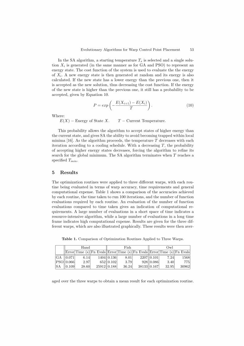
Evolutionary Algorithms for Warp Control Point Placement 53
In the SA algorithm, a starting temperature Ts is selected and a single solu-tion Xi is generated (in the same manner as for GA and PSO) to represent anenergy state. The cost function of the system is used to evaluate the the energyof Xi. A new energy state is then generated at random and its energy is alsocalculated. If the new state has a lower energy than the previous one, then itis accepted as the new solution, thus decreasing the cost function. If the energyof the new state is higher than the previous one, it still has a probability to beaccepted, given by Equation 10.
P = exp
(−E(Xi+1)− E(Xi)
T
). (10)
Where:E(X) − Energy of State X. T − Current Temperature.
This probability allows the algorithm to accept states of higher energy thanthe current state, and gives SA the ability to avoid becoming trapped within localminima [16]. As the algorithm proceeds, the temperature T decreases with eachiteration according to a cooling schedule. With a decreasing T , the probabilityof accepting higher energy states decreases, forcing the algorithm to refine itssearch for the global minimum. The SA algorithm terminates when T reaches aspecified Tmin.
5 Results
The optimization routines were applied to three different warps, with each rou-tine being evaluated in terms of warp accuracy, time requirements and generalcomputational expense. Table 1 shows a comparison of the accuracies achievedby each routine, the time taken to run 100 iterations, and the number of functionevaluations required by each routine. An evaluation of the number of functionevaluations compared to time taken gives an indication of computational re-quirements. A large number of evaluations in a short space of time indicates aresource-intensive algorithm, while a large number of evaluations in a long timeframe indicates high computational expense. Results are given for the three dif-ferent warps, which are also illustrated graphically. These results were then aver-
Table 1. Comparison of Optimization Routines Applied to Three Warps.
Hand Fish OwlError Time (s) Fn Evals Error Time (s) Fn Evals Error Time (s) Fn Evals
GA 0.071 6.14 1404 0.136 8.01 2207 0.101 7.24 1568PSO 0.066 2.97 652 0.102 3.79 928 0.086 3.40 775SA 0.109 28.60 25912 0.188 36.24 38133 0.167 32.95 30962
aged over the three warps to obtain a mean result for each optimization routine.
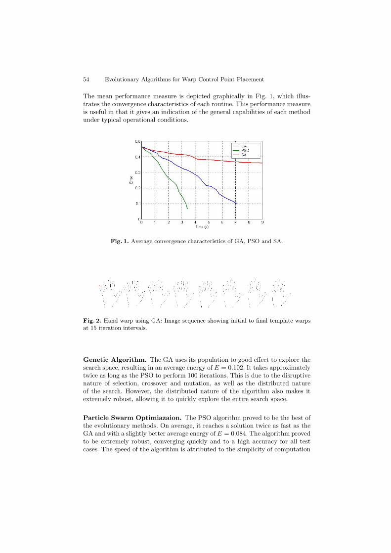
54 Evolutionary Algorithms for Warp Control Point Placement
The mean performance measure is depicted graphically in Fig. 1, which illus-trates the convergence characteristics of each routine. This performance measureis useful in that it gives an indication of the general capabilities of each methodunder typical operational conditions.
Fig. 1. Average convergence characteristics of GA, PSO and SA.
Fig. 2. Hand warp using GA: Image sequence showing initial to final template warpsat 15 iteration intervals.
Genetic Algorithm. The GA uses its population to good effect to explore thesearch space, resulting in an average energy of E = 0.102. It takes approximatelytwice as long as the PSO to perform 100 iterations. This is due to the disruptivenature of selection, crossover and mutation, as well as the distributed natureof the search. However, the distributed nature of the algorithm also makes itextremely robust, allowing it to quickly explore the entire search space.
Particle Swarm Optimiazaion. The PSO algorithm proved to be the best ofthe evolutionary methods. On average, it reaches a solution twice as fast as theGA and with a slightly better average energy of E = 0.084. The algorithm provedto be extremely robust, converging quickly and to a high accuracy for all testcases. The speed of the algorithm is attributed to the simplicity of computation
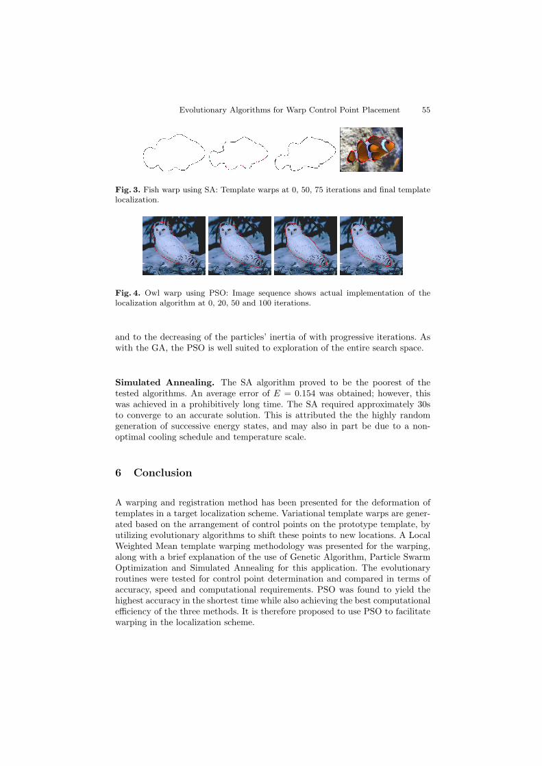
Evolutionary Algorithms for Warp Control Point Placement 55
Fig. 3. Fish warp using SA: Template warps at 0, 50, 75 iterations and final templatelocalization.
Fig. 4. Owl warp using PSO: Image sequence shows actual implementation of thelocalization algorithm at 0, 20, 50 and 100 iterations.
and to the decreasing of the particles’ inertia of with progressive iterations. Aswith the GA, the PSO is well suited to exploration of the entire search space.
Simulated Annealing. The SA algorithm proved to be the poorest of thetested algorithms. An average error of E = 0.154 was obtained; however, thiswas achieved in a prohibitively long time. The SA required approximately 30sto converge to an accurate solution. This is attributed the the highly randomgeneration of successive energy states, and may also in part be due to a non-optimal cooling schedule and temperature scale.
6 Conclusion
A warping and registration method has been presented for the deformation oftemplates in a target localization scheme. Variational template warps are gener-ated based on the arrangement of control points on the prototype template, byutilizing evolutionary algorithms to shift these points to new locations. A LocalWeighted Mean template warping methodology was presented for the warping,along with a brief explanation of the use of Genetic Algorithm, Particle SwarmOptimization and Simulated Annealing for this application. The evolutionaryroutines were tested for control point determination and compared in terms ofaccuracy, speed and computational requirements. PSO was found to yield thehighest accuracy in the shortest time while also achieving the best computationalefficiency of the three methods. It is therefore proposed to use PSO to facilitatewarping in the localization scheme.
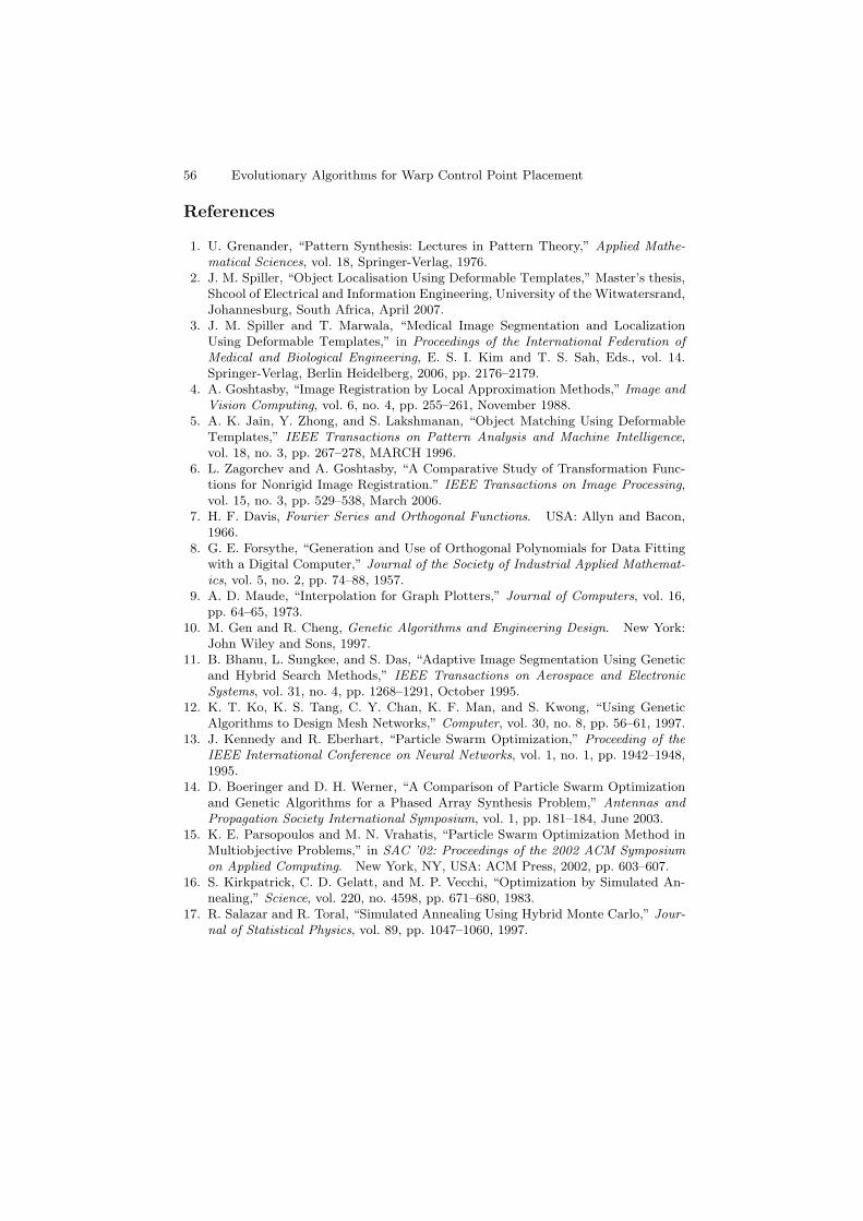
56 Evolutionary Algorithms for Warp Control Point Placement
References
1. U. Grenander, “Pattern Synthesis: Lectures in Pattern Theory,” Applied Mathe-matical Sciences, vol. 18, Springer-Verlag, 1976.
2. J. M. Spiller, “Object Localisation Using Deformable Templates,” Master’s thesis,Shcool of Electrical and Information Engineering, University of the Witwatersrand,Johannesburg, South Africa, April 2007.
3. J. M. Spiller and T. Marwala, “Medical Image Segmentation and LocalizationUsing Deformable Templates,” in Proceedings of the International Federation ofMedical and Biological Engineering, E. S. I. Kim and T. S. Sah, Eds., vol. 14.Springer-Verlag, Berlin Heidelberg, 2006, pp. 2176–2179.
4. A. Goshtasby, “Image Registration by Local Approximation Methods,” Image andVision Computing, vol. 6, no. 4, pp. 255–261, November 1988.
5. A. K. Jain, Y. Zhong, and S. Lakshmanan, “Object Matching Using DeformableTemplates,” IEEE Transactions on Pattern Analysis and Machine Intelligence,vol. 18, no. 3, pp. 267–278, MARCH 1996.
6. L. Zagorchev and A. Goshtasby, “A Comparative Study of Transformation Func-tions for Nonrigid Image Registration.” IEEE Transactions on Image Processing,vol. 15, no. 3, pp. 529–538, March 2006.
7. H. F. Davis, Fourier Series and Orthogonal Functions. USA: Allyn and Bacon,1966.
8. G. E. Forsythe, “Generation and Use of Orthogonal Polynomials for Data Fittingwith a Digital Computer,” Journal of the Society of Industrial Applied Mathemat-ics, vol. 5, no. 2, pp. 74–88, 1957.
9. A. D. Maude, “Interpolation for Graph Plotters,” Journal of Computers, vol. 16,pp. 64–65, 1973.
10. M. Gen and R. Cheng, Genetic Algorithms and Engineering Design. New York:John Wiley and Sons, 1997.
11. B. Bhanu, L. Sungkee, and S. Das, “Adaptive Image Segmentation Using Geneticand Hybrid Search Methods,” IEEE Transactions on Aerospace and ElectronicSystems, vol. 31, no. 4, pp. 1268–1291, October 1995.
12. K. T. Ko, K. S. Tang, C. Y. Chan, K. F. Man, and S. Kwong, “Using GeneticAlgorithms to Design Mesh Networks,” Computer, vol. 30, no. 8, pp. 56–61, 1997.
13. J. Kennedy and R. Eberhart, “Particle Swarm Optimization,” Proceeding of theIEEE International Conference on Neural Networks, vol. 1, no. 1, pp. 1942–1948,1995.
14. D. Boeringer and D. H. Werner, “A Comparison of Particle Swarm Optimizationand Genetic Algorithms for a Phased Array Synthesis Problem,” Antennas andPropagation Society International Symposium, vol. 1, pp. 181–184, June 2003.
15. K. E. Parsopoulos and M. N. Vrahatis, “Particle Swarm Optimization Method inMultiobjective Problems,” in SAC ’02: Proceedings of the 2002 ACM Symposiumon Applied Computing. New York, NY, USA: ACM Press, 2002, pp. 603–607.
16. S. Kirkpatrick, C. D. Gelatt, and M. P. Vecchi, “Optimization by Simulated An-nealing,” Science, vol. 220, no. 4598, pp. 671–680, 1983.
17. R. Salazar and R. Toral, “Simulated Annealing Using Hybrid Monte Carlo,” Jour-nal of Statistical Physics, vol. 89, pp. 1047–1060, 1997.
Chapter 3
Medical Image Segmentation and
Localization Using Deformable
Templates
This paper was presented at the World Congress on Medical Physics and Biomedical
Engineering in Seoul, Korea, in 2006. It presents a specific application of the localization
algorithm to functional medical images.
57
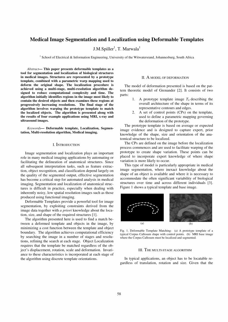
58
Medical Image Segmentation and Localization using Deformable Templates
J.M.Spiller1, T. Marwala
1
1 School of Electrical & Information Engineering, University of the Witwatersrand, Johannesburg, South Africa
Abstract— This paper presents deformable templates as a
tool for segmentation and localization of biological structures
in medical images. Structures are represented by a prototype
template, combined with a parametric warp mapping used to
deform the original shape. The localization procedure is
achieved using a multi-stage, multi-resolution algorithm de-
signed to reduce computational complexity and time. The
algorithm initially identifies regions in the image most likely to
contain the desired objects and then examines these regions at
progressively increasing resolutions. The final stage of the
algorithm involves warping the prototype template to match
the localized objects. The algorithm is presented along with
the results of four example applications using MRI, x-ray and
ultrasound images.
Keywords— Deformable template, Localization, Segmen-
tation, Multi-resolution algorithm, Medical imaging.
I. INTRODUCTION
Image segmentation and localization plays an important
role in many medical imaging applications by automating or
facilitating the delineation of anatomical structures. Since
all subsequent interpretation tasks, such as feature extrac-
tion, object recognition, and classification depend largely on
the quality of the segmented output, effective segmentation
has become a critical step for automated analysis in medical
imaging. Segmentation and localization of anatomical struc-
tures is difficult in practice, especially when dealing with
inherently noisy, low spatial resolution images such as those
produced using functional imaging.
Deformable Templates provide a powerful tool for image
segmentation, by exploiting constraints derived from the
image data together with a priori knowledge about the loca-
tion, size, and shape of the required structures [1].
The algorithm presented here is used to find a match be-
tween a deformed template and objects in the image, by
minimizing a cost function between the template and object
boundary. The algorithm achieves computational efficiency
by searching the image in a number of stages and resolu-
tions, refining the search at each stage. Object Localization
requires that the template be matched regardless of the ob-
ject’s displacement, rotation, scale and deformation. Invari-
ance to these characteristics is incorporated at each stage of
the algorithm using discrete template orientations.
II. A MODEL OF DEFORMATION
The model of deformation presented is based on the pat-
tern theoretic model of Grenander [2]. It consists of two
parts:
1. A prototype template image T0 describing the
overall architecture of the shape in terms of its
representative contours and edges.
2. A set of control points (CPs) on the template,
used to define a parametric mapping governing
the deformation of the prototype.
The prototype template is based on average or expected
image evidence and is designed to capture expert, prior
knowledge of the shape, size and orientation of the ana-
tomical structure to be localized.
The CPs are defined on the image before the localization
process commences and are used to facilitate warping of the
prototype to create shape variation. These points can be
placed to incorporate expert knowledge of where shape
variation is more likely to occur.
This type of model is particularly appropriate in medical
image segmentation, where inexact knowledge about the
shape of an object is available and where it is necessary to
accommodate the often significant variability of biological
structures over time and across different individuals [3].
Figure 1 shows a typical template and base image.
(a)
(b)
Fig. 1. Deformable Template Matching: (a) A prototype template of a
typical Corpus Callosum shape with control points. (b) MRI base image
where the Corpus Callosum must be localized and segmented.
III. THE MULTI-STAGE ALGORITHM
In typical applications, an object has to be locatable re-
gardless of translation, rotation and size. Given that the
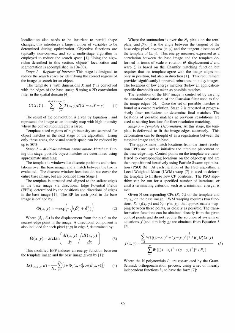
59
localization also needs to be invariant to partial shape
changes, this introduces a large number of variables to be
determined during optimization. Objective functions are
typically non-convex, and so a multi-stage algorithm is
employed to reduce the search space [1]. Using the algo-
rithm described in this section, objects’ localization and
segmentation is accomplished in 10s-30s.
Stage 1 – Regions of Interest: This stage is designed to
reduce the search space by identifying the correct regions of
the image to search for an object.
The template T with dimensions X and Y is convolved
with the edges of the base image B using a 2D convolution
filter in the spatial domain [4].
∑∑==
−−=)(
1
)(
1
),(),(),(Ysize
y
Xsize
x
yYxXByxTYXC (1)
The result of the convolution is given by Equation 1 and
represents the image as an intensity map with high intensity
where the convolution integral is large.
Template-sized regions of high intensity are searched for
object matches in the next stage of the algorithm. Using
only these areas, the visual search space can be reduced by
up to 80%.
Stage 2 – Multi-Resolution Approximate Matches: Dur-
ing this stage, possible object matches are determined using
approximate matching.
The template is windowed at discrete positions and orien-
tations over the base image, and a match between the two is
evaluated. The discrete window locations do not cover the
entire base image, but are obtained from Stage 1.
The template is attracted and aligned to the salient edges
in the base image via directional Edge Potential Fields
(EPFs), determined by the positions and directions of edges
in the base image [1]. The EP for each pixel in the base
image is defined by:
( ))(exp),( 22
yxyx δδ +−−=Φ (2)
Where (δx , δy) is the displacement from the pixel to the
nearest edge point in the image. A directional component is
also included for each pixel (x,y) in edge I, determined by:
=Θ
dx
yxdI
dy
yxdIyx
),(),(arctan),( (3)
This modified EPF induces an energy function between
the template image and the base image given by [1]:
( )∑=
Θ Φ+=TN
i
i
T
ds yxyxN
BTE1
,,, )),(cos(),(11
),( βζ (4)
Where the summation is over the NT pixels on the tem-
plate, and β(x, y) is the angle between the tangent of the
base edge pixel nearest (x, y) and the tangent direction of
the template at (x, y). This energy measure, expressed as a
correlation between the base image and the template de-
formed in terms of scale s, rotation Θ, displacement d and
warp ζ, is based on the Chamfer matching function but
requires that the template agree with the image edges not
only in position, but also in direction [1]. This requirement
provides significantly improved robustness in noisy images.
The locations of low energy matches (below an application-
specific threshold) are taken as possible matches.
The resolution of the EPF image is controlled by varying
the standard deviation σ, of the Gaussian filter used to find
the image edges [5]. Once the set of possible matches is
found at a coarse resolution, Stage 2 is repeated at progres-
sively finer resolutions to determine final matches. The
locations of possible matches at previous resolutions are
used as starting locations for finer resolution matching.
Stage 3 – Template Deformation: At this stage, the tem-
plate is deformed to fit the image edges accurately. This
deformation can be thought of as a registration between the
template image and the base.
The approximate match locations from the finest resolu-
tion EPFs are used to initialize the template placement on
the base edge-map. Control points on the template are trans-
ferred to corresponding locations on the edge-map and are
then repositioned iteratively using Particle Swarm optimiza-
tion (PSO) [6]. At each iteration of the PSO algorithm, a
Local Weighted Mean (LWM) warp [7] is used to deform
the template to fit these new CP positions. The PSO algo-
rithm can be run for a specified number of iterations, or
until a terminating criterion, such as a minimum energy, is
met.
Given N corresponding CPs (Xi, Yi) on the template and
(xi, yi) on the base image, LWM warping requires two func-
tions, Xi ≈ f(xi, yi) and Yi ≈ g(xi, yi), that approximate a map-
ping between these points, as closely as possible. The trans-
formation functions can be obtained directly from the given
control points and do not require the solution of systems of
equations. f (and similarly g) are obtained from Equation 5
[7].
∑
∑
=
=
−+−
−+−
=N
i
nii
N
i
inii
RyyxxW
yxPRyyxxW
yxf
1
2
1
22
1
2
1
22
}/])(){[(
),(}/])(){[(
),( (5)
Where the N polynomials Pi are constructed by the Gram-
Schmidt orthogonalization process, using a set of linearly
independent functions hi, to have the form [7]:
60
),(),(),(),(
),(),(),(),(
),(),(),(
),(),(
1100
2221210202
1110101
0000
yxhayxPayxPayxP
yxhayxPayxPayxP
yxhayxPayxP
yxhayxP
TTTTTT +++=
++=
+=
=
K
M
(6)
Where (x, y) is any arbitrary point in the image. The N
weight functions Wi are given by:
0)(
231)( 32
=
+−=
RW
RRRW
i
i
1
10
>
≤≤
R
R (7)
Where nii RyyxxR /])()[( 2
1
22 −+−= and nR is the
distance of point (xi, yi) from its (n-1)th
nearest control point
in the base image.
Apart from not requiring the solution of a system of
equations at each iteration, this LWM warp implementation
has a number of other advantages over alternate warp meth-
ods [8]:
• Corresponding control points are not mapped exactly to
each other so digital errors in the correspondences as
well as small mismatch errors are smoothed.
• The rational weight functions adapt to the density and
organization of the points and automatically extend to
large gaps between control points.
• Because varied placement of control points is accept-
able, expert knowledge of deformation can be incorpo-
rated.
The use of PSO to determine the optimal placement of
CPs is effective because the regions of the global minima
are known from Stage 2. To prevent the PSO from explor-
ing outside of these regions, and to limit warp dimensional-
ity, a penalty function is introduced that measures the sum
of the squared differences between CPs on the original and
deformed templates. The penalty function is added to the
energy cost given in Equation 4 and penalizes extreme
warps that would leave the region of the global minimum. It
is given by Equation 8, where α controls rigidity of the
warp.
∑=
−+−=N
x
iiii yYxXyxP1
22 )()(),( α (8)
IV. EXPERIMENTAL RESULTS
The deformable template model presented has been ap-
plied to different biological structures in a number of func-
tional medical images. All images were obtained from the
Tagare Medical Image Database [9].
The first test experiment presented involves the segmen-
tation of the Corpus Callosum in four different MRI images.
The prototype template used is the first Corpus Callosum
shape. This experiment is intended to illustrate the warp
capabilities of the algorithm, and the template image is
initialized at the center of the base images. Figure 2 shows
the initial and final base images. As can be seen, all four
Corpus Callosums are localized and segmented, even
though there is considerable shape variation between the
images.
(a)
(b)
Fig. 2. Corpus Callosum MRI images. (a) Original image. (b) Segmented
image.
The second experiment involves the detection of aneu-
rysms in ultrasound images. The search algorithm is illus-
trated in this experiment, where an aneurysm is detected in
two images regardless of template rotation and slight scale
change. The two segmented ultrasound images are shown
in Figure 3.
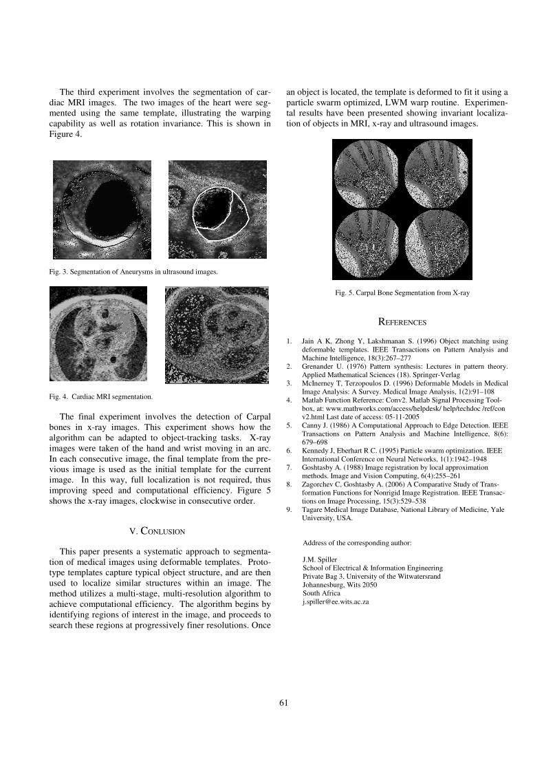
61
The third experiment involves the segmentation of car-
diac MRI images. The two images of the heart were seg-
mented using the same template, illustrating the warping
capability as well as rotation invariance. This is shown in
Figure 4.
Fig. 3. Segmentation of Aneurysms in ultrasound images.
Fig. 4. Cardiac MRI segmentation.
The final experiment involves the detection of Carpal
bones in x-ray images. This experiment shows how the
algorithm can be adapted to object-tracking tasks. X-ray
images were taken of the hand and wrist moving in an arc.
In each consecutive image, the final template from the pre-
vious image is used as the initial template for the current
image. In this way, full localization is not required, thus
improving speed and computational efficiency. Figure 5
shows the x-ray images, clockwise in consecutive order.
V. CONLUSION
This paper presents a systematic approach to segmenta-
tion of medical images using deformable templates. Proto-
type templates capture typical object structure, and are then
used to localize similar structures within an image. The
method utilizes a multi-stage, multi-resolution algorithm to
achieve computational efficiency. The algorithm begins by
identifying regions of interest in the image, and proceeds to
search these regions at progressively finer resolutions. Once
an object is located, the template is deformed to fit it using a
particle swarm optimized, LWM warp routine. Experimen-
tal results have been presented showing invariant localiza-
tion of objects in MRI, x-ray and ultrasound images.
Fig. 5. Carpal Bone Segmentation from X-ray
REFERENCES
1. Jain A K, Zhong Y, Lakshmanan S. (1996) Object matching using
deformable templates. IEEE Transactions on Pattern Analysis and
Machine Intelligence, 18(3):267–277
2. Grenander U. (1976) Pattern synthesis: Lectures in pattern theory.
Applied Mathematical Sciences (18). Springer-Verlag
3. McInerney T, Terzopoulos D. (1996) Deformable Models in Medical
Image Analysis: A Survey. Medical Image Analysis, 1(2):91–108
4. Matlab Function Reference: Conv2. Matlab Signal Processing Tool-
box, at: www.mathworks.com/access/helpdesk/ help/techdoc /ref/con
v2.html Last date of access: 05-11-2005
5. Canny J. (1986) A Computational Approach to Edge Detection. IEEE
Transactions on Pattern Analysis and Machine Intelligence, 8(6):
679–698
6. Kennedy J, Eberhart R C. (1995) Particle swarm optimization. IEEE
International Conference on Neural Networks, 1(1):1942–1948
7. Goshtasby A. (1988) Image registration by local approximation
methods. Image and Vision Computing, 6(4):255–261
8. Zagorchev C, Goshtasby A. (2006) A Comparative Study of Trans-
formation Functions for Nonrigid Image Registration. IEEE Transac-
tions on Image Processing, 15(3):529–538
9. Tagare Medical Image Database, National Library of Medicine, Yale
University, USA.
Address of the corresponding author:
J.M. Spiller
School of Electrical & Information Engineering
Private Bag 3, University of the Witwatersrand
Johannesburg, Wits 2050
South Africa