Embed Size (px)
Citation preview

Object Detection andDense Captioning
You Only Look Once: Unified, Real-Time ObjectDetection. Joseph Redmon, Santosh Divvala,
Ross Girshick, Ali Farhadi, CVPR 2016
DenseCap: Fully Convolutional LocalizationNetworks for Dense Captioning. Justin Johnson,
Andrej Karpathy, Li Fei-Fei, CVPR 2016
Dana Berman and Guy Leibovitz
January 2, 2017

Faster R-CNN
I Region ProposalNetwork (RPN)
• Anchor boxes(xa, ya,wa, ha)
• Predict:k × (tx , ty , tw , th)
x = xa + txwa
w = wa exp(tw)
I ROI pooling → classifierand bbox regression

Faster R-CNN - Limitations
I Training:
• NIPS 2015:alternatingoptimization
• arXiv 2016:end-to-end(approximately)
I Not real-time:0.2sec/image

YOLO

YOLO - Overview
I You only look once
I Trainable end-to-end

YOLO - MethodInput image

YOLO - MethodImage is split into a gridWe split the image into a grid

YOLO - MethodEach cell predicts boxes and confidences: P(object)Each cell predicts boxes and confidences: P(Object)

YOLO - MethodEach cell predicts boxes and confidences: P(object)Each cell predicts boxes and confidences: P(Object)

YOLO - MethodEach cell predicts boxes and confidences: P(object)Each cell predicts boxes and confidences: P(Object)
YOLO - MethodEach cell also predicts a class probabilityEach cell also predicts a class probability.

YOLO - MethodClass probability is conditional: P(class|object)Each cell also predicts a class probability.
Dog
Bicycle Car
Dining Table

YOLO - MethodCombining the box and class predictionsThen we combine the box and class predictions.

YOLO - MethodNon-Maximal Suppression and threshold detectionsFinally we do NMS and threshold detections

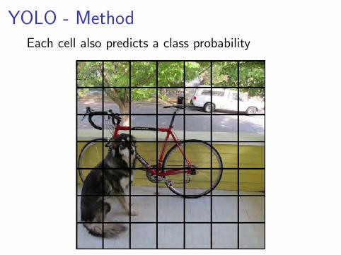
YOLO - MethodThe output size is fixed.Each cell predicts:
I B bounding boxes. For each bounding box:I 4 coordinates (x , y ,w , h)I 1 confidence value P(object)
I N class probabilities P(class|object)
YOLO - MethodEach cell predicts:
- For each bounding box:- 4 coordinates (x, y, w, h)- 1 confidence value
- Some number of class probabilities
For Pascal VOC:
- 7x7 grid- 2 bounding boxes / cell- 20 classes
7 x 7 x (2 x 5 + 20) = 7 x 7 x 30 tensor = 1470 outputs
This parameterization fixes the output size
For Pascal VOC:
I 7× 7 grid
I B = 2 bounding boxes / cell
I N = 20 classes
7× 7× (2× 5 + 20) = 7× 7× 30 tensor

YOLO - MethodNeural Network

YOLO - MethodInspired by Inception from GoogLeNet

YOLO - MethodInception module (CVPR 2015):

YOLO - MethodOne neural network is trained to be the wholedetection pipeline

YOLO - MethodTraining:
I Pre-training conv. layers on ImageNet,using low-res input (1 week)
I For detection: add layers, increase imageresolution
I Normalize bounding box coordinates to [0, 1]
I Data augmentation: random scale, translation,exposure and saturation
I Loss function: L2

YOLO - MethodLoss function:

YOLO - FrameworkDarknet - Open source neural networks in Chttp://pjreddie.com/darknet/
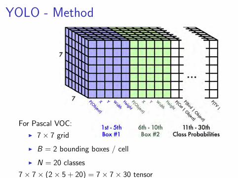
YOLO - ResultsExample of results on natural images:
YOLO works across a variety of natural images

YOLO - ResultsIt also generalizes well to new domains (such as art):
It also generalizes well to new domains (like art)

YOLO - ResultsQuantitative detection and localization results:

YOLO - ResultsLimitations:
I Small objects
I Unusual aspect ratios
I Multiple objects per grid cell

Beyond YOLO
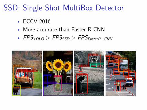
SSD: Single Shot MultiBox Detector
I ECCV 2016
I More accurate than Faster R-CNN
I FPSYOLO > FPSSSD > FPSFasterR−CNN

YOLO9000: Better, Faster, Stronger
I arXiv, 25 Dec 2016
I 9000 object classes

Lessons from SSD and YOLO9000
I Multi-scale feature mapsI Predict anchor box offsets
I NormalizedI h ∼ ha exp(t)I Aspect ratios
I Data augmentation (scale, brightness, etc.)

Dense Captioning

Background: Detection and CaptioningComputer Vision Tasks

Background: Visual Genome DatasetVisual Genome Dataset
108,077 images 5,408,689 regions + captions
Krishna et al, "Visual Genome", 2016
A boy wearing
jeans
A red tricycle
A red flying frisbeeTwo men playing frisbee
Wooden privacy fence
The ground is made of stone
The legsof a man
An athletic shoe on a foot

Overview
Questions?Justin Johnson*, Andrej Karpathy*, Li Fei-Fei
Stanford University
DenseCap: Fully Convolutional Localization Networks for Dense Captioning
Abstract Fully Convolutional Localization and Captioning Architecture Region Search by Text Query
Dense Captioning Results
Quantitative Evaluation
Task. We introduce the dense captioning task, which requires a computer vision system to both localize and describe salient regions in images in natural language. The dense captioning task generalizes object detection when the descriptions consist of a single word, and Image Captioning when one predicted region covers the full image. Model. To address the localization and description task jointly we propose a Fully Convolutional Localization Network (FCLN) architecture that processes an image with a single, efficient forward pass, requires no external regions proposals, and can be trained end-to-end with a single round of optimization. The architecture is composed of a Convolutional Network, a novel dense localization layer, and Recurrent Neural Network language model that generates the label sequences. Experiments. We evaluate our network on the Visual Genome dataset, which comprises 94,000 images and 4,100,000 region-grounded captions. We observe both speed and accuracy improvements over baselines based on current state of the art approaches in both generation and retrieval settings.
Dense Captioning task
Model Description (broken down)
Classification
Cat
Captioning
A cat riding a skateboard
Detection
Cat
Skateboard
Dense CaptioningOrange spotted cat
Skateboard with red wheels
Cat riding a skateboard
Brown hardwood flooring
label densityWhole Image Image Regions
label complexity
SingleLabel
Sequence
CNN
Image: 3 x W x H Conv features:
C x W’ x H’
Region features:B x C x X x Y Region Codes:
B x D
LSTMStriped gray cat
Cats watching TV
Localization Layer
Conv
Region Proposals:4k x W’ x H’
Region scores:k x W’ x H’Conv features:
C x W’ x H’Bilinear Sampler Region features:
B x 512 x 7 x 7
Sampling Grid:B x X x Y x 2
Sampling Grid Generator
Best Proposals:B x 4
Recognition Network
Faster R-CNN: Towards Real-Time Object Detection with Region Proposal Networks, Ren et al., NIPS 2015Spatial Transformer Networks, Jaderberg et al., NIPS 2015
white tennis shoes head of a giraffe red and white sign hands holding a phone
front wheelof a bus
A man and a woman sitting at a table with a cake. A train is traveling down the tracks near a forest.A large jetliner flying through a blue sky. A teddy bear with
a red bow on it.
Our Model:
Full Image RNN:
Image Retrieval by Bag of Text Queries
Better performance (5.39 vs. 4.26 mAP) 13X faster. Runs @ 4-20fps
Open Source Code ReleaseFind the code on Github!https://github.com/jcjohnson/densecap
- A pretrained model- Code to run the model on new images, on either CPU or GPU- Code to run a live demo with a webcam- Evaluation code for dense captioning- Instructions for training the model
Stop by poster #2!

Spatial Transformer Networks
(a) (b)
Figure 3: Two examples of applying the parameterised sampling grid to an image U producing the output V .(a) The sampling grid is the regular grid G = TI(G), where I is the identity transformation parameters. (b)The sampling grid is the result of warping the regular grid with an affine transformation T✓(G).For clarity of exposition, assume for the moment that T✓ is a 2D affine transformation A✓. We willdiscuss other transformations below. In this affine case, the pointwise transformation is
✓xs
i
ysi
◆= T✓(Gi) = A✓
0@
xti
yti
1
1A =
✓11 ✓12 ✓13
✓21 ✓22 ✓23
�0@
xti
yti
1
1A (1)
where (xti, y
ti) are the target coordinates of the regular grid in the output feature map, (xs
i , ysi ) are
the source coordinates in the input feature map that define the sample points, and A✓ is the affinetransformation matrix. We use height and width normalised coordinates, such that �1 xt
i, yti 1
when within the spatial bounds of the output, and �1 xsi , y
si 1 when within the spatial bounds
of the input (and similarly for the y coordinates). The source/target transformation and sampling isequivalent to the standard texture mapping and coordinates used in graphics [8].
The transform defined in (10) allows cropping, translation, rotation, scale, and skew to be appliedto the input feature map, and requires only 6 parameters (the 6 elements of A✓) to be produced bythe localisation network. It allows cropping because if the transformation is a contraction (i.e. thedeterminant of the left 2⇥ 2 sub-matrix has magnitude less than unity) then the mapped regular gridwill lie in a parallelogram of area less than the range of xs
i , ysi . The effect of this transformation on
the grid compared to the identity transform is shown in Fig. 3.
The class of transformations T✓ may be more constrained, such as that used for attention
A✓ =
s 0 tx0 s ty
�(2)
allowing cropping, translation, and isotropic scaling by varying s, tx, and ty . The transformationT✓ can also be more general, such as a plane projective transformation with 8 parameters, piece-wise affine, or a thin plate spline. Indeed, the transformation can have any parameterised form,provided that it is differentiable with respect to the parameters – this crucially allows gradients to bebackpropagated through from the sample points T✓(Gi) to the localisation network output ✓. If thetransformation is parameterised in a structured, low-dimensional way, this reduces the complexityof the task assigned to the localisation network. For instance, a generic class of structured and dif-ferentiable transformations, which is a superset of attention, affine, projective, and thin plate splinetransformations, is T✓ = M✓B, where B is a target grid representation (e.g. in (10), B is the regu-lar grid G in homogeneous coordinates), and M✓ is a matrix parameterised by ✓. In this case it ispossible to not only learn how to predict ✓ for a sample, but also to learn B for the task at hand.
3.3 Differentiable Image Sampling
To perform a spatial transformation of the input feature map, a sampler must take the set of samplingpoints T✓(G), along with the input feature map U and produce the sampled output feature map V .
Each (xsi , y
si ) coordinate in T✓(G) defines the spatial location in the input where a sampling kernel
is applied to get the value at a particular pixel in the output V . This can be written as
V ci =
HX
n
WX
m
U cnmk(xs
i � m;�x)k(ysi � n;�y) 8i 2 [1 . . . H 0W 0] 8c 2 [1 . . . C] (3)
4

Spatial Transformer Networks
]
] ]
]
U V
Localisation net
Sampler
Spatial Transformer
Grid !generator
]T✓(G)✓
Figure 2: The architecture of a spatial transformer module. The input feature map U is passed to a localisationnetwork which regresses the transformation parameters ✓. The regular spatial grid G over V is transformed tothe sampling grid T✓(G), which is applied to U as described in Sect. 3.3, producing the warped output featuremap V . The combination of the localisation network and sampling mechanism defines a spatial transformer.
need for a differentiable attention mechanism, while [14] use a differentiable attention mechansimby utilising Gaussian kernels in a generative model. The work by Girshick et al. [11] uses a regionproposal algorithm as a form of attention, and [7] show that it is possible to regress salient regionswith a CNN. The framework we present in this paper can be seen as a generalisation of differentiableattention to any spatial transformation.
3 Spatial TransformersIn this section we describe the formulation of a spatial transformer. This is a differentiable modulewhich applies a spatial transformation to a feature map during a single forward pass, where thetransformation is conditioned on the particular input, producing a single output feature map. Formulti-channel inputs, the same warping is applied to each channel. For simplicity, in this section weconsider single transforms and single outputs per transformer, however we can generalise to multipletransformations, as shown in experiments.
The spatial transformer mechanism is split into three parts, shown in Fig. 2. In order of computation,first a localisation network (Sect. 3.1) takes the input feature map, and through a number of hiddenlayers outputs the parameters of the spatial transformation that should be applied to the feature map– this gives a transformation conditional on the input. Then, the predicted transformation parametersare used to create a sampling grid, which is a set of points where the input map should be sampled toproduce the transformed output. This is done by the grid generator, described in Sect. 3.2. Finally,the feature map and the sampling grid are taken as inputs to the sampler, producing the output mapsampled from the input at the grid points (Sect. 3.3).
The combination of these three components forms a spatial transformer and will now be describedin more detail in the following sections.
3.1 Localisation Network
The localisation network takes the input feature map U 2 RH⇥W⇥C with width W , height H andC channels and outputs ✓, the parameters of the transformation T✓ to be applied to the feature map:✓ = floc(U). The size of ✓ can vary depending on the transformation type that is parameterised,e.g. for an affine transformation ✓ is 6-dimensional as in (10).
The localisation network function floc() can take any form, such as a fully-connected network ora convolutional network, but should include a final regression layer to produce the transformationparameters ✓.
3.2 Parameterised Sampling Grid
To perform a warping of the input feature map, each output pixel is computed by applying a samplingkernel centered at a particular location in the input feature map (this is described fully in the nextsection). By pixel we refer to an element of a generic feature map, not necessarily an image. Ingeneral, the output pixels are defined to lie on a regular grid G = {Gi} of pixels Gi = (xt
i, yti),
forming an output feature map V 2 RH0⇥W 0⇥C , where H 0 and W 0 are the height and width of thegrid, and C is the number of channels, which is the same in the input and output.
3
(a) (b)
Figure 3: Two examples of applying the parameterised sampling grid to an image U producing the output V .(a) The sampling grid is the regular grid G = TI(G), where I is the identity transformation parameters. (b)The sampling grid is the result of warping the regular grid with an affine transformation T✓(G).For clarity of exposition, assume for the moment that T✓ is a 2D affine transformation A✓. We willdiscuss other transformations below. In this affine case, the pointwise transformation is
✓xs
i
ysi
◆= T✓(Gi) = A✓
0@
xti
yti
1
1A =
✓11 ✓12 ✓13
✓21 ✓22 ✓23
�0@
xti
yti
1
1A (1)
where (xti, y
ti) are the target coordinates of the regular grid in the output feature map, (xs
i , ysi ) are
the source coordinates in the input feature map that define the sample points, and A✓ is the affinetransformation matrix. We use height and width normalised coordinates, such that �1 xt
i, yti 1
when within the spatial bounds of the output, and �1 xsi , y
si 1 when within the spatial bounds
of the input (and similarly for the y coordinates). The source/target transformation and sampling isequivalent to the standard texture mapping and coordinates used in graphics [8].
The transform defined in (10) allows cropping, translation, rotation, scale, and skew to be appliedto the input feature map, and requires only 6 parameters (the 6 elements of A✓) to be produced bythe localisation network. It allows cropping because if the transformation is a contraction (i.e. thedeterminant of the left 2⇥ 2 sub-matrix has magnitude less than unity) then the mapped regular gridwill lie in a parallelogram of area less than the range of xs
i , ysi . The effect of this transformation on
the grid compared to the identity transform is shown in Fig. 3.
The class of transformations T✓ may be more constrained, such as that used for attention
A✓ =
s 0 tx0 s ty
�(2)
allowing cropping, translation, and isotropic scaling by varying s, tx, and ty . The transformationT✓ can also be more general, such as a plane projective transformation with 8 parameters, piece-wise affine, or a thin plate spline. Indeed, the transformation can have any parameterised form,provided that it is differentiable with respect to the parameters – this crucially allows gradients to bebackpropagated through from the sample points T✓(Gi) to the localisation network output ✓. If thetransformation is parameterised in a structured, low-dimensional way, this reduces the complexityof the task assigned to the localisation network. For instance, a generic class of structured and dif-ferentiable transformations, which is a superset of attention, affine, projective, and thin plate splinetransformations, is T✓ = M✓B, where B is a target grid representation (e.g. in (10), B is the regu-lar grid G in homogeneous coordinates), and M✓ is a matrix parameterised by ✓. In this case it ispossible to not only learn how to predict ✓ for a sample, but also to learn B for the task at hand.
3.3 Differentiable Image Sampling
To perform a spatial transformation of the input feature map, a sampler must take the set of samplingpoints T✓(G), along with the input feature map U and produce the sampled output feature map V .
Each (xsi , y
si ) coordinate in T✓(G) defines the spatial location in the input where a sampling kernel
is applied to get the value at a particular pixel in the output V . This can be written as
V ci =
HX
n
WX
m
U cnmk(xs
i � m;�x)k(ysi � n;�y) 8i 2 [1 . . . H 0W 0] 8c 2 [1 . . . C] (3)
4
V ci =
H∑
n
W∑
m
Ucnmk(x si −m)k(y si − n)

∇ Spatial Transformer Networks
where �x and �y are the parameters of a generic sampling kernel k() which defines the imageinterpolation (e.g. bilinear), U c
nm is the value at location (n, m) in channel c of the input, and V ci
is the output value for pixel i at location (xti, y
ti) in channel c. Note that the sampling is done
identically for each channel of the input, so every channel is transformed in an identical way (thispreserves spatial consistency between channels).
In theory, any sampling kernel can be used, as long as (sub-)gradients can be defined with respect toxs
i and ysi . For example, using the integer sampling kernel reduces (3) to
V ci =
HX
n
WX
m
U cnm�(bxs
i + 0.5c � m)�(bysi + 0.5c � n) (4)
where bx + 0.5c rounds x to the nearest integer and �() is the Kronecker delta function. Thissampling kernel equates to just copying the value at the nearest pixel to (xs
i , ysi ) to the output location
(xti, y
ti). Alternatively, a bilinear sampling kernel can be used, giving
V ci =
HX
n
WX
m
U cnm max(0, 1 � |xs
i � m|) max(0, 1 � |ysi � n|) (5)
To allow backpropagation of the loss through this sampling mechanism we can define the gradientswith respect to U and G. For bilinear sampling (5) the partial derivatives are
@V ci
@U cnm
=HX
n
WX
m
max(0, 1 � |xsi � m|) max(0, 1 � |ys
i � n|) (6)
@V ci
@xsi
=HX
n
WX
m
U cnm max(0, 1 � |ys
i � n|)
8<:
0 if |m � xsi | � 1
1 if m � xsi
�1 if m < xsi
(7)
and similarly to (7) for @V ci
@ysi
.
This gives us a (sub-)differentiable sampling mechanism, allowing loss gradients to flow back notonly to the input feature map (6), but also to the sampling grid coordinates (7), and therefore backto the transformation parameters ✓ and localisation network since @xs
i
@✓ and @xsi
@✓ can be easily derivedfrom (10) for example. Due to discontinuities in the sampling fuctions, sub-gradients must be used.This sampling mechanism can be implemented very efficiently on GPU, by ignoring the sum overall input locations and instead just looking at the kernel support region for each output pixel.
3.4 Spatial Transformer Networks
The combination of the localisation network, grid generator, and sampler form a spatial transformer(Fig. 2). This is a self-contained module which can be dropped into a CNN architecture at any point,and in any number, giving rise to spatial transformer networks. This module is computationally veryfast and does not impair the training speed, causing very little time overhead when used naively, andeven speedups in attentive models due to subsequent downsampling that can be applied to the outputof the transformer.
Placing spatial transformers within a CNN allows the network to learn how to actively transformthe feature maps to help minimise the overall cost function of the network during training. Theknowledge of how to transform each training sample is compressed and cached in the weights ofthe localisation network (and also the weights of the layers previous to a spatial transformer) duringtraining. For some tasks, it may also be useful to feed the output of the localisation network, ✓,forward to the rest of the network, as it explicitly encodes the transformation, and hence the pose, ofa region or object.
It is also possible to use spatial transformers to downsample or oversample a feature map, as one candefine the output dimensions H 0 and W 0 to be different to the input dimensions H and W . However,with sampling kernels with a fixed, small spatial support (such as the bilinear kernel), downsamplingwith a spatial transformer can cause aliasing effects.
5
where �x and �y are the parameters of a generic sampling kernel k() which defines the imageinterpolation (e.g. bilinear), U c
nm is the value at location (n, m) in channel c of the input, and V ci
is the output value for pixel i at location (xti, y
ti) in channel c. Note that the sampling is done
identically for each channel of the input, so every channel is transformed in an identical way (thispreserves spatial consistency between channels).
In theory, any sampling kernel can be used, as long as (sub-)gradients can be defined with respect toxs
i and ysi . For example, using the integer sampling kernel reduces (3) to
V ci =
HX
n
WX
m
U cnm�(bxs
i + 0.5c � m)�(bysi + 0.5c � n) (4)
where bx + 0.5c rounds x to the nearest integer and �() is the Kronecker delta function. Thissampling kernel equates to just copying the value at the nearest pixel to (xs
i , ysi ) to the output location
(xti, y
ti). Alternatively, a bilinear sampling kernel can be used, giving
V ci =
HX
n
WX
m
U cnm max(0, 1 � |xs
i � m|) max(0, 1 � |ysi � n|) (5)
To allow backpropagation of the loss through this sampling mechanism we can define the gradientswith respect to U and G. For bilinear sampling (5) the partial derivatives are
@V ci
@U cnm
=
HX
n
WX
m
max(0, 1 � |xsi � m|) max(0, 1 � |ys
i � n|) (6)
@V ci
@xsi
=
HX
n
WX
m
U cnm max(0, 1 � |ys
i � n|)
8<:
0 if |m � xsi | � 1
1 if m � xsi
�1 if m < xsi
(7)
and similarly to (7) for @V ci
@ysi
.
This gives us a (sub-)differentiable sampling mechanism, allowing loss gradients to flow back notonly to the input feature map (6), but also to the sampling grid coordinates (7), and therefore backto the transformation parameters ✓ and localisation network since @xs
i
@✓ and @xsi
@✓ can be easily derivedfrom (10) for example. Due to discontinuities in the sampling fuctions, sub-gradients must be used.This sampling mechanism can be implemented very efficiently on GPU, by ignoring the sum overall input locations and instead just looking at the kernel support region for each output pixel.
3.4 Spatial Transformer Networks
The combination of the localisation network, grid generator, and sampler form a spatial transformer(Fig. 2). This is a self-contained module which can be dropped into a CNN architecture at any point,and in any number, giving rise to spatial transformer networks. This module is computationally veryfast and does not impair the training speed, causing very little time overhead when used naively, andeven speedups in attentive models due to subsequent downsampling that can be applied to the outputof the transformer.
Placing spatial transformers within a CNN allows the network to learn how to actively transformthe feature maps to help minimise the overall cost function of the network during training. Theknowledge of how to transform each training sample is compressed and cached in the weights ofthe localisation network (and also the weights of the layers previous to a spatial transformer) duringtraining. For some tasks, it may also be useful to feed the output of the localisation network, ✓,forward to the rest of the network, as it explicitly encodes the transformation, and hence the pose, ofa region or object.
It is also possible to use spatial transformers to downsample or oversample a feature map, as one candefine the output dimensions H 0 and W 0 to be different to the input dimensions H and W . However,with sampling kernels with a fixed, small spatial support (such as the bilinear kernel), downsamplingwith a spatial transformer can cause aliasing effects.
5

Losses Dense Captioning Architecture
Convolutional Network
Recurrent Network
Localization Layer
Recognition Network
Joint training: Minimize five losses
1. Box regression (position) 2. Box classification (confidence)3. Box regression (position) 4. Box classification (confidence)5. Captioning

Captioning RNNDense Captioning: Prior Work
Region Proposals
Crop
Convolutional Network
START man throwing disc
man throwing disc END
START red frisbee
red frisbee END
START gray stone ground
gray stone ground END
Recurrent NetworkKarpathy and Fei-Fei, CVPR 2015

Results
18
black computer monitorman wearing a blue shirt
sitting on a chair
people are in the background
computer monitor on a desk
silver handle on the wall
man with black hair
black bag on the floor
red and brown chair
wall is white

Additional Application - Finding RegionsGiven Description
21
Finding regions given descriptions“head of a giraffe”
0.1
0.10.2
0.90.9
0.4
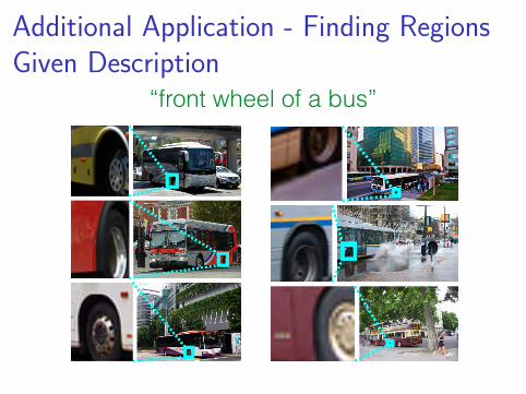
Additional Application - Finding RegionsGiven Description
24
“front wheel of a bus”Finding regions given descriptions