Object Classification from Acoustic Analysis of Impact

Robert S. Durst Eric P. Krotkov

CMU-RI-TR-93-16

The Robotics Instime Camegie Melloo University

Pittsburgh, Pennsylvania 15213

June 1993

Q 1993 Camegie Melloo University

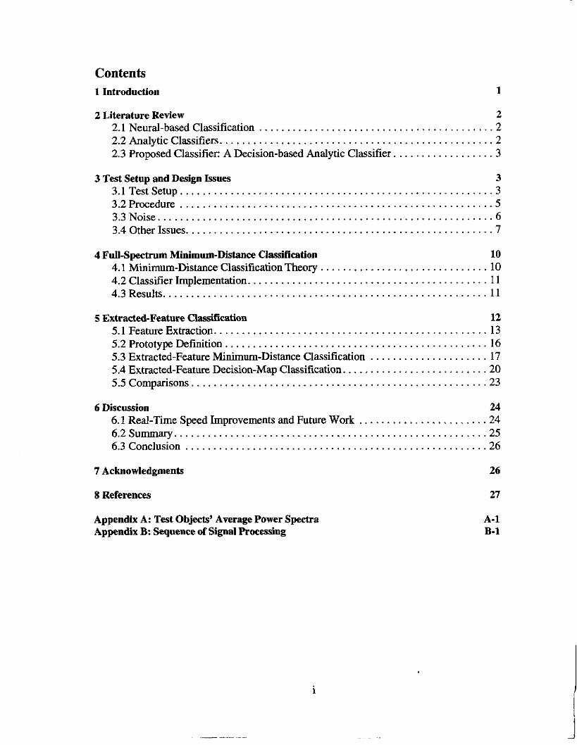
Contents 1 Introduction 1

2 Literature Review 2 2.1 Neural-based Classification .......................................... 2 2.2 Analytic Classifiers . . . . . . . . . . . . . . . . . . . . . . . . . . . . . . . . . . . . . . . . . . . . . . . . . 2 2.3 Proposed Classifier: A Decision-based Analytic Classifier . . . . . . . . . . . . . . . . . . 3

3 3.1TestSetup . . . . . . . . . . . . . . . . . . . . . . . . . . . . . . . . . . . . . . . . . . . . . . . . . . . . . . . . 3 3.2Procedure . . . . . . . . . . . . . . . . . . . . . . . . . . . . . . . . . . . . . . . . . . . . . . . . . . . . . . . . 5 3.3Noise ............................................................ 6 3.4 Other Issues ....................................................... 7

4 Full-Spectrum Minimum-Distance CLassiBcation 10

3 Test Setup and Design Issues

4.1 Minimum-Distance Classification Theory .............................. 10 4.2 Classifier Implementation ........................................... 11 4.3 Results .......................................................... 11

5 Extracted-Feature Classification 12 5.1 Feature Extraction ................................................. 13 5.2 Prototype Definition ............................................... 16 5.3 Extracted-Feature Minimum-Distance Classification ..................... 17 5.4 Extracted-Feature Decision-Map Classification .......................... 20 5.5 Comparisons . . . . . . . . . . . . . . . . . . . . . . . . . . . . . . . . . . . . . . . . . . . . . . . . . . . . . 23

6 Discussion 24 6.1 Real-Time Speed Improvements and Future Work ....................... 24 6.2Su mmary ........................................................ 25 6.3 Conclusion ...................................................... 26

7 Acknowledgments 26

8 References 27

Appendix A: Test Objects’ Average Power Spectra Appendix B: Sequence of Signal Processing

i

...

A-1 B-1

.. 11

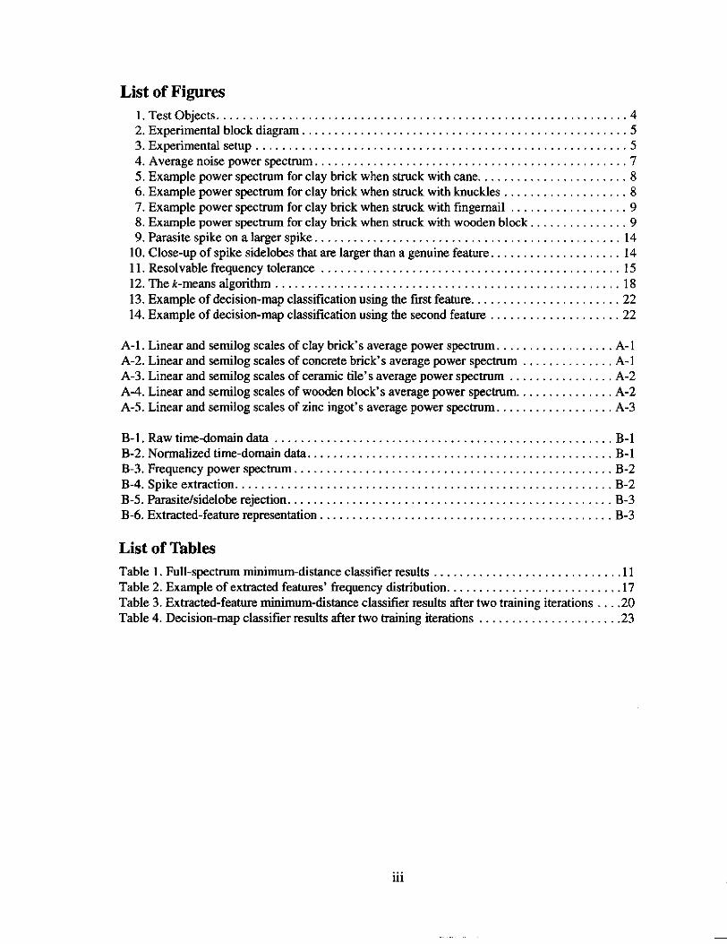
List of Figures 1. Testobjects . . . . . . . . . . . . . . . . . . . . . . . . . . . . . . . . . . . . . . . . . . . . . . . . . . . . . . . . . . . . . . . 4 2 . Experimental block diagram .................................................. 5 3.Experimentalsetup ......................................................... 5 4 . Average noise power spectrum ................................................ 7 5 . Example power spectrum for clay brick when struck with cane ....................... 8 6 . Example power spectrum for clay brick when struck with knuckles . . . . . . . . . . . . . . . . . . . 8 7 . Example power spectrum for clay brick when struck with fingernail . . . . . . . . . . . . . . . . . . 9 8 . Example power spectrum for clay brick when struck with wooden block . . . . . . . . . . . . . . . 9 9 . Parasite spike on a larger spike ............................................... 14

10 . Close-up of spike sidelobes that are larger than a genuine feature .................... 14 11 . Resolvable frequency tolerance .............................................. 15 12 . The k-means algorithm ..................................................... 18 13 . Example of decision-map classification using the first feature ....................... 22 14 . Example of decision-map classification using the second feature .................... 22

A-1 . Linear and semilog scales of clay brick‘s average power spectrum . . . . . . . . . . . . . . . . . . A- 1 A-2 . Linear and semilog scales of concrete brick‘s average power spectrum . . . . . . . . . . . . . . A-1 A-3 . Linear and semilog scales of ceramic tile’s average power spectrum . . . . . . . . . . . . . . . . A-2 A 4 . Linear and semilog scales of wooden block‘s average power spectrum . . . . . . . . . . . . . . . A-2 A-5 . Linear and semilog scales of zinc ingd’s average power spectrum . . . . . . . . . . . . . . . . . . A-3

B-1.Rawtimedomaindata .................................................... B-1 B-2 . Normalized time-domain data ............................................... B-1 B-3 . Frequency power spectrum ................................................. B-2 B-4.Spikeextraction .......................................................... B-2 B-5 . Parasitehidelobe rejection .................................................. B-3 B-6 . Extracted-feature representation ............................................. B-3

List of Tables Table 1 . Full-spectrum minimum-distance classifier results ............................. 11 Table 2 . Example of extracted features’ frequency distribution ........................... 17 Table 3 . Extracted-feature minimum-distance classifier results after two training iterations . . . 2 0 Table 4 . Decision-map classifier results after two training iterations ..................... 2 3

... 111

Abstract

We address the problem of autonomously classifying objects from the sounds they make when struck, and present results from different attempts to classify various items.

Previous work has shown that object classification is possible based on features derived from the frequency content of signals. We develop a moving-maximum algo- rithm to extract the two most significant spikes in the FFT of the sounds of impact, and use these extracted spikes as features. We describe the transformation of the training data’s extracted features into a compilation of representative cluster means. These cluster means are used as labeled inputs to the different classifiers discussed.

We discuss two techniques to classify test vectors based on their extracted feature spikes, and show that accurate classification of objects is possible using these features. The first technique is the familiar minimumdistance classifier that calculates the dis- tance between a given test vector and each cluster mean, and assigns the test vector to the cluster that yields the smallest error. The second technique is one we developed for the task: the decision-map clussijkr: a hybrid minimum-distance classifier and deci- sion-tree classifier, that iteratively finds the closest cluster mean to each test vector and uses multiple features only if it cannot classify the test sample.

Results from classifier trials show that using our moving-maximum feature extractor and decision-map classifier, object classification from the sound of impact can be done as accurately as using the minimum-distance classifier, but at significantly lower com- putational expense.

1

1 Introduction Imagine knocking on two doors, one wood and one metal. People can easily tell which door is which, even if they look the same, based on the sound they make. The purpose of this work is to take the first steps toward enabling machines to do this as well. This has potential applications where other methods, such as vision or force sensing, may fail. One such application is in non-destructive testing: research has been done concerning in situ acoustic detection of defects, but where structures located in hostile environments need to be examined, machines capable of identifying faults can accomplish this task without jeopardizing human safety.

We are interested in the problem of using the sound of impact to learn about the composition of objects. Specifically, we want to see if it is possible to accurately classify different objects based on the sounds they make when struck. Essentially, this is a signal processing and pattern recognition problem. Previous work has shown that acoustic-based classification of certain signals, depending on the application, is feasible using either frequency or time- domain models. We propose to use spikes in the signal‘s frequency spectrum as feature vectors.

One of this project’s design paradigms was simplicity, so we show that classification is possible using a simple minimum-distance classifier. This sort of classification scheme compares a test vector to a prototype vector for each labeled class, calculates the distance between the two samples for every class, and assigns the test vector to the class whose prototype yields the lowest error. We use an obvious prototype definition- the representative vector for each class is simply the mean of the training samples’ spectra. Experimental results suggest that using entire spectra as feature vectors may lead to poor classifier performance, so we develop a featw-extraction algorithm that identifies the N most significant frequency spikes and compiles the class means based on these extracted features.

In addition to the feature-extraction algorithm, we also develop the decision-map classifier, a variant on the standard minimumdistance classifier scheme. The decision-map classifier iteratively finds the nearest class prototypes to the test vector and assigns the test vector to the same class as the closest matching prototype. Preliminary results indicate that both the minimum-distance and decision-map classifiers can accurately classify objects based on the feature-extracted data, demonstrating that object classification from the sound of impact is indeed possible. Furthermore, we propose that the decision-map classifier has a computational advantage over the minimum-distance classifier. The minimum-distance technique calculates the N-dimensional distance between vectors (where Nis the number of features), while the decision-map calculates distance using only as many features as necessary to unequivocally find the closest class prototype. This can result in a significant reduction in computational complexity compared to the miniiumdistance classifier, making the decision-map classifier an attractive alternative.

In order to function autonomously, robots must have some way of extracting information from their surroundings and then applying that information to perform specific tasks. Specifically, the ability to do classification given raw data is an important step towards

n L

machine intelligence. We address the problem of sound-based object classification and speculate that the establishment of a knowledge base of many different objects' acoustic properties can provide clues to help robots infer general material properties about its environment from acoustic tests. This paper provides a necessary starting point for this area of research.

2 Literature Review Previous work has dealt with both analytically-based classifiers (based on mathematical properties of the data) and learning heuristic classifiers (trainable neural networks), and these techniques offer their own advantages to given problems. Acknowledging that classifier performance is not only dependent on the choice of the classifier itself but also on the test data, certain kinds of classifiers are more ideally suited to some problems than to others.

2.1 Neural-based Classication Legitimus and Schwab [2] showed that both a multilayer perceptron (MLP) and an Adaline- like-network performed very well for the problem of classifying underwater transients, but only after significant preprocessing to extract features; the MLYs success rate on raw data was barely better than chance. The authors also showed that the neural network classifiers outperformed an analytical classifier (a factorial discriminant analysis classifier) and a simpler clustering classifier- so called because it looks for natural aggregation within classes and natural separation between classes and assigns test samples to the most similar cluster.

Beck et al. [3] showed that a hybrid classifier composed of two different kinds of classifiers outperformed either type alone, on a set of sample data. Two neural nets, a MLP and a radial basis function (RBF) were tested, along with classical analytic classifiers, the K-nearest neighbor (KNN) and the Fisher linear discriminant function. Each classifier worked perfectly on the training data, but could not reliably classify the test data. The authors found that a parallel implementation of RBF and MLP networks led to perfect classification, as long as the features extracted from the data were chosen carefully. The graph of results from their trials suggests that a hybrid MLPFisher discriminant classifier would yield similar results; again, however, the extracted features must be chosen carefully. The authors note that they got the best results using WVL3 wavelet representation.

2.2 Analytic Classifiers Stewart and Larson [4] addressed the problem of extracting features for classifying objects- in this case, aircraft- based on acoustic emissions. Their feature extraction technique was to observe the spectral content of the signal over time and look for stationary frequencies whose amplitudes exceeded a defined threshold. This has the advantage of weeding out spurious signals, but is computationally expensive to calculate the spectrogram and pick out and analyze time slices of interest. After defining the relevant features, the authors suggested that an appropriate classifier would be a template-matching scheme, which can be implemented as a nearest-neighbor classifier.

3

Perron [5 ] addressed the issue of acoustic classification of feature-reduced signals by proposing a decision tree instead of more analytical or learning-based classifiers. Her conclusion was that decision trees can perform reasonably well and offer a “natural“ classification scheme; that is, one that is more conceptually tangible (and therefore, more physically meaningful to human intelligibility) than abstractions like linear discriminant functions. A moment’s reflection by the reader should confirm thi- people tend to look for obvious differences in discriminating between objects, and this is a direct implementation of a decision tree algorithm: i j it’s block-shaped, rhen it could be a brick or a box; if it’s solid, then it’s a brick.

2.3 Proposed Classier: A Decision-based Analytical Classifier This report describes the decision-map classifier and frequency-domain feature extractor. When taken together, they comprise a classification system that includes elements from the techniques mentioned in Section 2.2: feature extraction based on the N most significant frequency components and classification using a template matching scheme, implemented as a decision-directed minimum-distance classifier. As a driving goal of this research was simplicity, we tried to find the easiest, most logical and most natural way of processing data, extracting features and implementing the classifier. To this end, [4] pmvides the motivation for using a minimum-distance scheme, and [ 5 ] bolsters the natural-interpretation concept underlying the decision map design.

In the final implementation, the decision-map classifier compares test vectors and class prototypes based on the single most significant feature and assigns the test sample to the nearest-neighbor prototype. If a single nearest match cannot be found, the classifier uses the next most significant feature in each vector and repeats the process until it finds a single matching class. It then assigns the test vector to this class. We hypothesize that this decision- based minimum-distance classifier, used in conjunction with our feature-extraction algorithm, can accurately identify each object based on the sound of impact, and will provide a necessary step toward enabling machines to “hear” the compositions of their surroundings.

3 Test Setup and Design Goals Our classification design paradigm was as simple as possible: take many samples of each class, define a prototype for each class based on this training data, and then compare a test vector to the prototype. Thus the true design problems were how to define the prototype and how to do the comparisons. As with any supervised classification scheme, design of the algorithm depends on at least a cursory review of some sample data, so this section describes the test setup and some of the significant characteristics of the data and its analysis.

3.1 Test Setup A guiding hypothesis has been that the power spectrum of the sound of a struck object is sufficient to classify that object. Therefore, the test vectors and prototypes were ultimately derived from frequency characteristics of various data taken.

4

Figure 1. Objects tested in this research project Clockwise. from top left mer: wooden block, concrete brick, clay brick, zinc ingot. ceramic tile.

Five test objects were used

standard clay brick, 7'12" x 3'12" x 2'fc

standard concrete brick, 7'/2" x 3l/$ x 2'14''

small square ceramic tile, 4 '/; x 4'/27, x '/< wooden block, 6 '/$ x 33/," x 1'/;

irregularly-shaped zinc ingot, roughly T x 43/c x 1''

The hardware used included an aluminum cane with a I: stic ti^ which was 3pped onto the test objects; an omnidirectional electret condenser microphone element mounted with amplification circuitry on a circuit boar& a 1TE 40dB Series low-pass filter (proprietary design); and an Intel-80386-based PC with a Keithley Metrabyte DAS-20 A D board, and running Keithley's EasyEST data acquisition and data processing software. The DAS-20's top sample rate was experimentally found to be about 70kHz.

The basic block diagram is shown in Figure 2, and the actual experimental setup is shown in Figure 3. Data was taken by placing a microphone near the object under test, striking it with a cane, and recording the sound of impact. The data was triggered on a rising edge greater than 0.01V and sampled at 40 kHz. To prevent aliasing, a low-pass filter with a -3 dB cutoff frequency of 17.5 kHz and a -40 dB (minimum) cutoff frequency of 22.75 kHz; this was

5

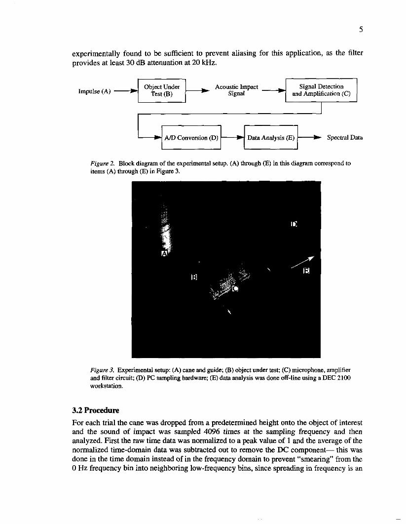
experimentally found to be sufficient to prevent aliasing for this application, as the filter provides at least 30 dB attenuation at 20 kHz.

Object Under Acoustic Impact Signal Detection Impulse (A) and Amplification (C)

AID Conversion @) Data Analysis @) + Spectral Data

Figure 2. Block diagram of the experimental setup. (A) through (E) in this diagram correspond to items (A) through (E) in Figure 3.

Figure 3. Experimental setup: (A) cane and guide; (B) object under test; (C) microphone, amplifier and filter circuit; @) PC sampling bardware; (E) data analysis was done off-line using a DEC 2100 workstation.

3.2 Procedure For each trial the cane was dropped from a predetermined height onto the object of interest and the sound of impact was sampled 4096 times at the sampling frequency and then analyzed. First the raw time data was normalized to a peak value of 1 and the average of the normalized time-domain data was subtracted out to remove the DC component- this was done in the time domain instead of in the frequency domain to prevent “smearing” from the 0 Hz frequency bin into neighboring low-frequency bins, since spreading in frequency is an

inevitable result of taking the Fourier transform of windowed data.’ After normalization and bias removal, the data was windowed with a Hannhg function2 and then the 4096-point fast Fourier transform was taken and stored as a power spectrum, an array with strictly real elements, whose values are the magnitudes of the complex values of each point in the returned FFT.

The raw time-domain data was normalized for the sake of 2-D clustering, using frequency and amplitude as coordinates. By scaling all the data to the same size, the relative amplitudes between frequency components are preserved and clustered together, regardless of what the absolute amplitudes are. For example, suppose. that object X consistently emits a sound whose two main spikes are 2000 Hz and 2400 Hz, and the 2000 Hz spike is always 15 dB higher than the 2400 Hz spike. If object X is struck repeatedly at a variety of amplitudes, the main frequency components will also take on a range of amplitudes, so the high-amplitude 2000 Hz spikes will be more than 15 dB greater than the low-amplitude 2400 Hz spikes. This introduces spread in amplitude and will make classification that is based on spike amplitudes more difficult. However, if the raw data is first normalized, only the relative amplitudes are preserved, and all of the 2400 Hz spikes will again be 15 dB below the 2000 Hz spikes.

3.3 Noise As the microphone element was very sensitive, once the data was triggered the sampling hardware logged everyhng the microphone could pick up. Ideally, this would be only the fading sound of the impact, and this data could be spectrally analyzed and significant spikes could be identified. This brings up the question of noise: how can we ensure that the spikes accepted as features are components of the signal from the struck object and not from environmental or channel noise?

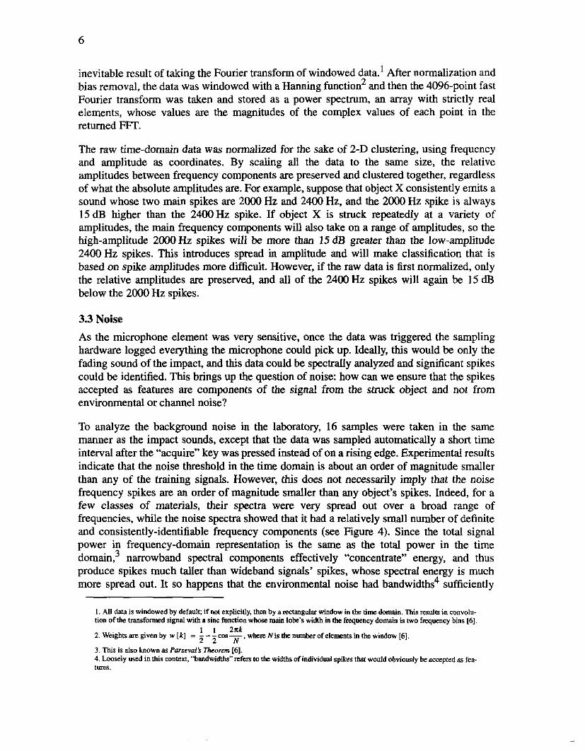
To analyze the background noise in the laboratory, 16 samples were taken in the same manner as the impact sounds, except that the data was sampled automatically a short time interval after the “acquire” key was pressed instead of on a rising edge. Experimental results indicate that the noise threshold in the time domain is about an order of magnitude smaller than any of the training signals. However, this does not necessarily imply that the noise frequency spikes are an order of magnitude smaller than any object’s spikes. Indeed, for a few classes of materials, their spectra were very spread out over a broad range of frequencies, while the noise spectra showed that it had a relatively small number of definite and consistently-identifiable frequency components (see Figure 4). Since the total signal power in frequency-domain representation is the same as the total power in the time domain? narrowband spectral components effectively “concentrate” energy, and thus produce spikes much taller than wideband signals’ spikes, whose spectral energy is much more spread out. It so happens that the environmental noise had bandwidths4 sufficiently

I . All data is windowed by default: ifnat explicitly, them by B ~ g u l a r w h d o r v in the ti= domain. This mulb in convolu- tion ofthe transformed signal with a sinc fundion whose main lobc’s width in the frequency domain i s two frequency bins [6].

1 1 2rk 2.Weighaarpgivenby wLk1 = ---cos-,wwherpNis~nnlonberofelem;nainthewindaw[6].

3 . This i s also known as Porsevdk Theorem [61. 4. Lmsely used in this Conlcxt, “ b a n d w i W rcfers to the widths of individual spiltes that would obviomly bc accepted 85 fea- t W .

2 2 N

7

1. .

w 1 ~ 3

I [ I I

,.-I . L

2.m

0.50

narrow such that the spikes were occasionally taller than those of some wideband signals, and so noise frequencies were sometimes identified as features. Qpically, however, the objects’ signal frequencies were different from noise frequencies, and so the noise could be identified and ignored.

3.4 Other Issues The above paragraph showed that background noise in the laboratory, while numerically significant, could nevertheless be ignored. However, there is a more subtle point that still needs to be addressed on the subject of noise- not the random noise inherent in the system, and not the laboratory background noise, but the causal noise in the signal: how can we distinguish the sound generated by the object from the sound generated by the cane? This section shows that the test objects remain identifiable even when struck with different canes.

We tried to predict what the sound of impact should be under ideal conditions, first by trying to calculate the sound waves emitted by the object based on its composition and shape and then verifying that the experimentally-derived features were close to the predicted values. Some work had been done in this area on a theoretical basis; Kac [7] and Fisher [SI focused on the case of vibrating membranes, which are analyzed much more simply than vibrating rigid objects. Kac suggested that it was not possible to unequivocally infer the topology of the membrane’s bounded edge based on the sound of impact, unless this edge was a circle. Fisher was a little more optimistic, and suggested that it was indeed possible to infer the shape of the membrane, but only if the membrane’s isotropic or anisotropic structure was known.

As we did not know the molecular structure of the test objects, we tried to experimentally determine what frequencies belonged to the objects by looking at intra-class comparisons using diyerent canes: common features between trials using the same material and different canes imply representative object features. Four objects (clay and concrete bricks, tile and

8

1.50

1.00 -

0.50 -

0.00

zinc block) were tested using four canes (aluminum cane with a plastic tip, a wooden block, knuckles and fingernails).

- . I

1.50

1.00 -

0.50 -

0.00 - . I

0.00 5.00 10.00 15.00 20.w

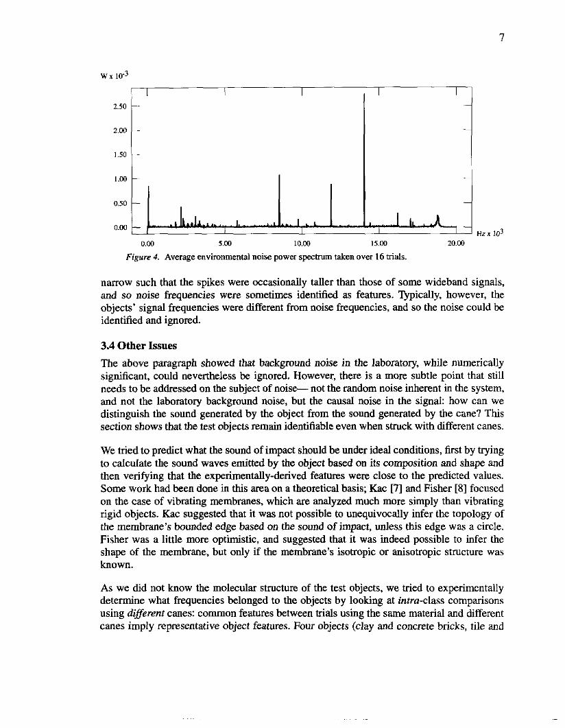
Figure 5. Example of the clay brick's power spectrum when stiuck by the aluminum cane with a plastic tip. Specuurn is auncated at 2OomW m show detail. The most significant exaacted frequency is 2686 Hz, and the second most significant extracted frequency is 6182 Hz.

I I I I I HE x 103 I I I I I HE x 103

800.00

1w.00

m.00

500.00

400.00

300.00

200.00

100.00

0.00

0.00 5.w 10.00 15.00 20.00

Figure 6. Example of the clay brick's power spectrum when struck with knuckles. Spectrum is truncated at 2oOmW to scale to Figure 5. The most significant extracted frequency is 2686 Hz, the same as in Figure 5.

- I I I I I - -

- - I - -

- 1 - - - - - - - -

. i I I I I H e x l d

While each object produced spectra whose major component frequencies changed as the cane changed, it was nevertheless impossible to show that the different canes produced the different frequencies. Every object exhibited&quencyjitter, a slight change in frequency of the main spike, across many trials using the same cane. The best-behaved objects, so called because they produced the most consistently-identifiable spectra, showed frequency jitter of

800.00

1w.00

m.00

500.00

400.00

300.00

200.00

100.00

0.00

- I I I I I - -

- - I - -

- 1 - - - - - - - -

. i I I I I H e x l d

9

100

0.80

0.60

0.40

0.20

0.00

I I I 1 I 1

. , I I I H~ 103

-

-

-

-

-

a00 5.00 10.00 15.00 20.00

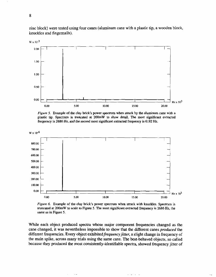
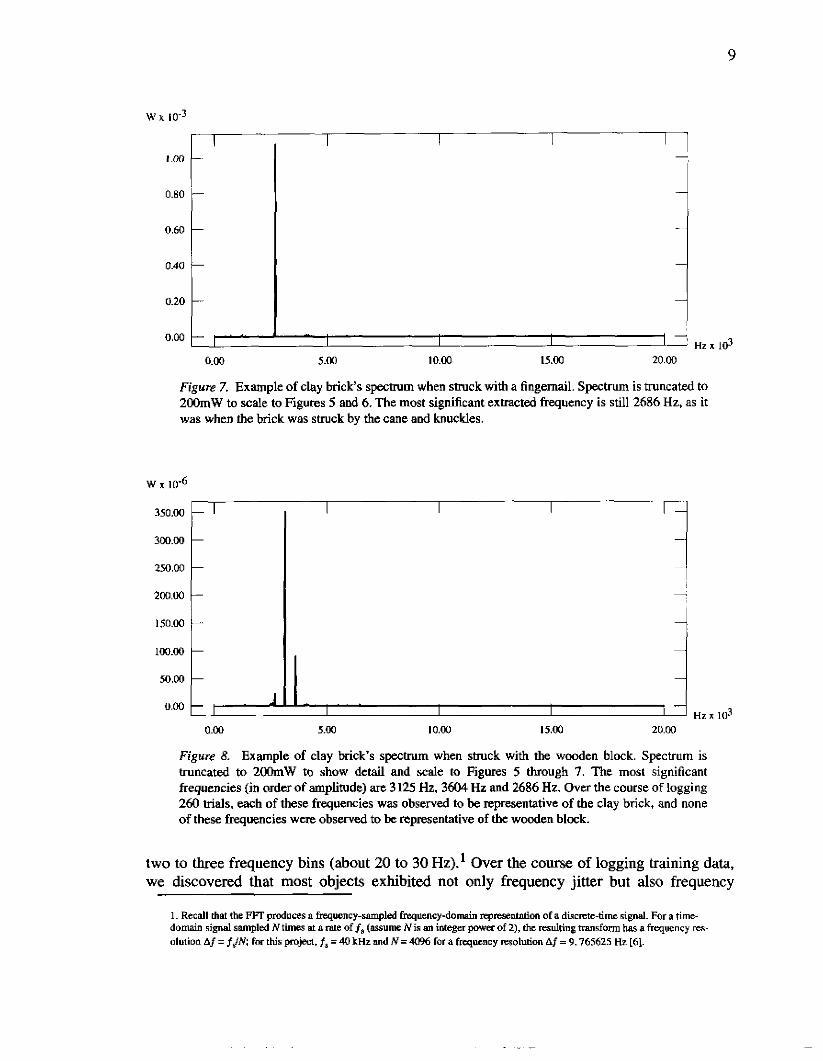
Figure 7. Example of clay brick's s-rn when stluck with a fingernail. Spectrum is truncated to 2OOmW to scale to Figures 5 and 6. The most significant extracted frequency is still 2686 Hz, as it was when the brick was struck by the cane and knuckles.

w x 10-6

0.m 5.00 10.00 15.00 20.00

Figure 8. Example of clay brick's spectrum when struck with the wooden block. Spectrum is truncated to 2oOmW to show detail and scale to Figures 5 through 7. The most significant frequencies (in order of amplitude) are 3 125 Hz, 3604 Hz and 2686 Hz. Over the course of logging 260 bids, each of these frequencies was observed to be representative of the clay brick, and none of these frequencies were observed to be representative of the wooden block.

two to three frequency bins (about 20 to 30 Hz).' Over the course. of logging training data, we discovered that most objects exhibited not only frequency jitter but also frequency

1. Recall that the Wl' produces a frequency-sampled hquency-domain xprcsentation o i a discme-time signal. For a time- domain signalsampledNtimsata~off,(assumNis~integerpwrerof2),thcnsultin~transformhasafrequen~yres ohtion Af = fJN iwthispmjea.f,=40~andN=4096iarafrequcncyresolutionAf =9.765625 Hz[61.

10

scatter: the most significant spike in one hit might be completely different- on the order of thousands of hertz- from the main spike in another hit within the same class; we observed this even when trying to hit the objects consistently. For this reason, the results shown in Figures 5 through 8 suggest that the objects emit their representative frequencies regardless of the cane used to strike them.

Because the only significant frequencies emitted by the best-behaved objects using different canes were the same major frequencies emitted in other trials using the same cane, and because analyzing the crystal structure of the test objects was well beyond the scope of this project, we judged this particular problem to be intractable and assumed that, at least for a small number of significant features, the sound of the cane was not significant compared to the sound of the object.

4 Full-Spectrum Minimum-Distance Classification By comparing the various objects’ example frequency data in Figures A-1 through A-5 (Appendix A), it should be apparent that the simplest classifier is a frequency-based one, since the frequency content of different materials appears to be distinct. This implies an obvious classifier: compare a test object’s entire spectrum with a representative spectrum for each class, and assign the object to the class which provides the closest spectral match. At this brute-force level, the nearest-neighbor (or rninimurn-disrunce) classifier is simple both conceptually and in practice.

4.1 Minimum-Distance Classification Theory In classical nearest-neighbor a test vector is compared with each labeled training sample and is assigned to the same class as the “closest matching” training vector. The concept of a “closest match” usually means some kind of distance measure in feature space, onto which each vector (both test and prototype) is projected. As a simple case, suppose we want to classify several vectors in %’. An obvious feature space is exactly s3, since each element of each vector can be considered a feature of that vector.

If the number of labeled training samples is large, comparing every test sample with every k n i n g sample becomes impractical. In this case minimum-distance classification can be done by comparing test samples with prototypes for each class. An intuitive choice for a class prototype is the class mean (or the cluster mean). Given a set of labeled training data, each vector y, in class ci is assumed to lie in the same general region (a clmter) in the feature space as every other member of ci. and the arithmetic mean of the entire population of cj is the cluster mean pi:

where y’ is the j* vector in ci and Ni is the number of vectors yi, Note that calling p the “cluster mean” as opposed to the “class mean” implies that the vectors in each class are expected to automatically cluster together; this is not necessarily the case.

‘j

Finally, error, or distance, is defined. Duda and Hart [9] note several different distance schemes, some intuitive and some creative. Typically, distance between vectors is simply defined as the Euclidean distance, or

training data 11 20/30 I 18/30 I 23130

(2) 2 T d; = ( x - L q (x--ll$

where x and pi are column vectors and di is a scalar. Going back to the s3 example in Section 4.1, the distance di between the test column vector x and another three-dimensional column vector ~i is

30130 I 19/30 11 1101150

where, again, di is a scalar and xk and pik denote the kh scalar elements of vectors x and pi, respectively.

4.2 Classifier Implementation We used a minimum-distance scheme with a mean-squared error measure (a scaled Euclidean distance measure) as the error criterion, class means as the prototypes and entire spectra as test vectors. The 4096-point FFT returns a 2049-length vector whose indices are frequency bins and whose elements are amplitudes, implying a 2049-dimensional feature space. Training samples for each of five classes were taken by carefully striking each object in the same location 30 times, and these samples were normalized, unbiased, transformed and then averaged' to create the class means. f i e same training samples were then compared with the prototypes for each class and the resulting distance measures were used as final criteria for the classifier: the test vector was assigned to the class that produced the lowest distance measure. We used the training data as a check for the classifier: because the prototypes were. developed directly and only from the training data, the classifier should perform best on training data, and poor performance in this case virtually guarantees even worse performance on test data.

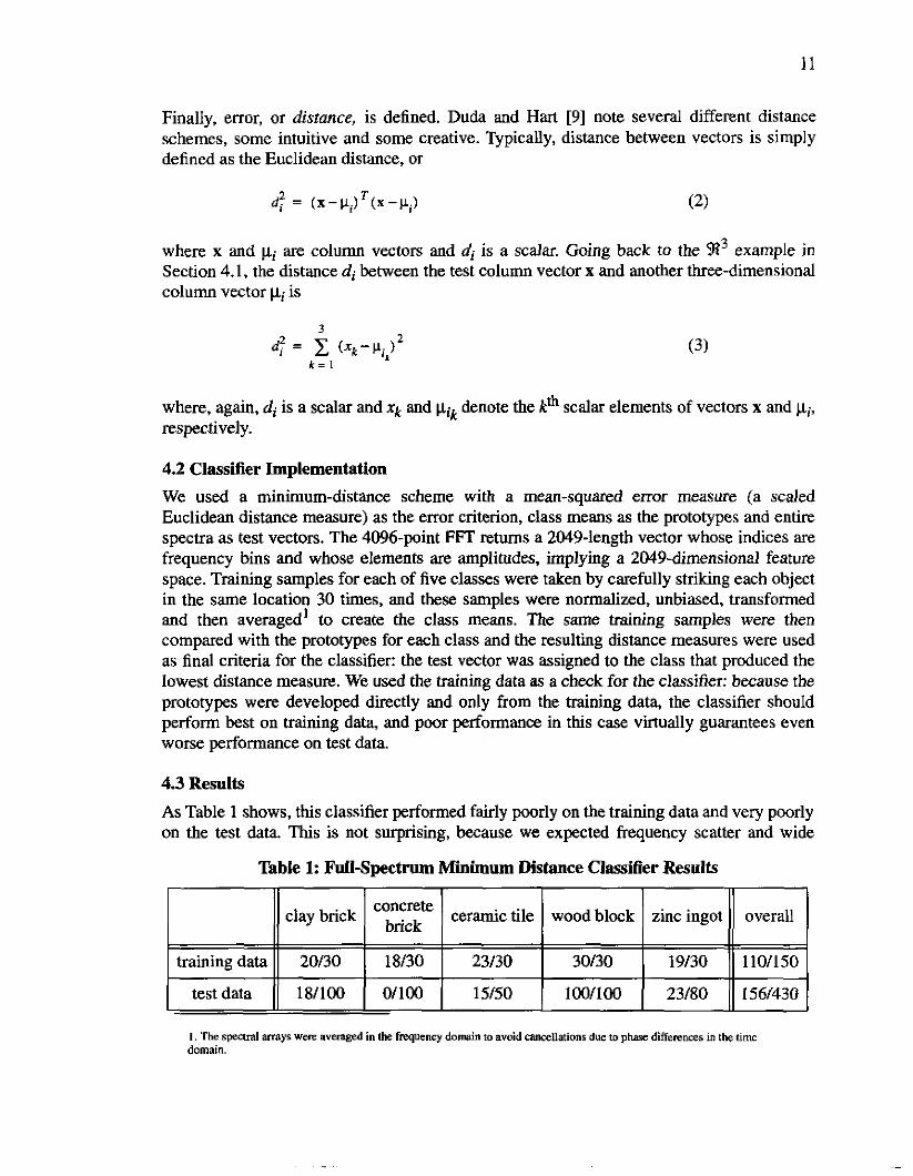
4.3 Results As Table 1 shows, this classifier performed fairly poorly on the training data and very poorly on the test data. This is not surprising, because we expected frequency scatter and wide

Table 1: Full-Spectrum Minimum Distance Classifier Results I 1 I I I I I1 I

test data

I ll I concrete 1) clay brick 1 brick 1 ceramic tile I wood block zinc ingot overall

18/100 0/100 15/50 I00/100 23/80 156/430 I

12

variability in amplitude to create large errors. What is surprising is that it performed as we11 as it did on the training data, and on the wooden block in general. Disregarding the results for wood, the dismal performance for the other four classes indicates that this method is a poor choice for a classifier. Furthermore, that the classifier performs so well on wood while performing so poorly on the other materials suggests that either the wooden block radiates a spectrum whose intraclass variation is low relative to the other objects’, or that there is something wrong with this classifier.

Experimental evidence from logging hundreds of samples has shown that the best-behaved objects exhibit some frequency jitter and significant swings in amplitude in their major spikes. As objects get less well-behaved, they produce frequency scatter and less reproducible spectra, increasing their intraclass variation. Analysis of all of the training and test data suggests that the clay and concrete bricks are the best-behaved objects, while wood is probably the worst. For the minimum mean-squared error classifier to work well on wood alone suggests that it was less a matter of finding the prototype with the best fit than finding the prototype with a low-valued spectrum for all frequencies. Each of the other objects produced sharp, distinct spikes that towered over the surrounding spectra, so energy was concentrated in these spikes and minimized elsewhere. Wood, on the other hand, had a more spread spectrum, with energy distributed over a broad range of frequencies, and so the “spikes” (to be precise, the values of each frequency bin) were forced to be smaller.

In order to test this hypothesis, the wood block’s training data was tested against two random noise samples, one that was uniformly-distributed and one that was normally- distributed. The noise samples were transformed into frequency-domain representation and then scaled such that their total energies were equal to the total energy in wood‘s prototype (this was done instead of normalization because the amplitude of the raw-time random data did not decay over time, unlike the test objects’ time-domain data, so the total energy in the random samples was greater than the energy in wood’s). Out of the 130 training and test samples for wood, it correctly classified only 42, which is no better than chance. These results, coupled with the results for the other materials, confirm that the full-spectrum minimum-distance classifier is insufficient to classify objects based on their acoustic spectra.

5 Extracted-Feature Classification Since the full-spectrum method did not work, we turned to a more sophisticated breed of classifiers and tried to correct the problems that plagued the basic minimum-distance classifier. The drawback to the bruteforce method was a wide dynamic range between samples. Between classes, large absolute differences in amplitude across all frequencies is expected this is what produces large errors when material X is compared with prototype Y. Wide swings in amplitude are nut expected between members of the same class, however, and comparatively moderate differences in amplitude between main spikes may be over an order of magnitude greater than any other spectral component, and thus overwhelm the less significant spikes’ contributions to the classification scheme. This should not happen for materials that consistently radiate predictable frequencies at predictable relative intensities, but even the best-behaved objects under observation exhibited variations in frequency, and

13

these variations, coupled with the sharpness of the peaks, could lead to the type of large differences in spike amplitude as described above.

Figures A-1 through A-5 indicate that the objects emit certain frequencies unique to themselves, which suggests that amplitude differences are not relevant for this line of research. Thus if only the significant frequencies were identified and all else rejected, classification still would be possible. The problem now is to extract the most significant frequencies so we can use these parameters as the classifier’s input data.

5.1 Feature Extraction Extracted-feature classifiers require that a prohibitively large datum (for example, a vector or a signal) be distilled into a meaningful but much smaller representation. Typically, the goal is to model a complex signal as a much simpler signal that can be described by unique parameters, or features. For example, a @,q) +rde.r auto-regressive-moving-average (ARMA) model that minimizes the mean-squared difference between a signal and its estimate can be defined by p+q parameters. These parameters, instead of the entire signal, can be used as input data to the classifier [5 ] .

[3] and [5 ] showed that classifier performance depends not only on how the classifier is defined but also on what features are used. Therefore, cafe must also be taken to ensure that the features used to model the data are appropriate. As the power spectra of our sample data showed consistent frequency components (at least for some classes), it seemed fitting that features be chosen from the frequency-domain representation. The simplest and most intuitive feature-extraction scheme was to take the N tallest spikes in the power spectrum and use their coordinates (in amplitude and frequency) as inputs to the classifier.

For implementation’s sake, a computer had to be programmed to recognize a spike from a non-spike, and to recognize a feature from a non-feature- “spike” and “feature” are not synonymous. The simplest definition of a spike is any data point whose value is greater than both of its neighbors, but spike identification of this sort also picked out “parasitic” spikes: those data points that were spikes in their own right on a microscopic scale but were also obviously part of a macroscopic trend that defined a much larger spike (see Figure 9). Thus we needed a way to smooth out these parasites, which for classification purposes were not signijcunf spikes (that is, potential features). A simple weighted moving-average filter effectively smoothed out small parasites while preserving the significant spikes.

The other problem was to distinguishbetween features and non-features. Originally we used a rectangular window to minimize frequency spread when transforming the time-domain data into the frequency domain. However, this created large sidelobes, and for certain classes of objects, these sidelobes were much taller than other frequency components. Thus additional preprocessing was required to reject sidelobes. An immediate solution was to use a different window for the FFT- we selected a Hanning window, which gave good sidelobe suppression. Still, for spikes whose amplitudes were orders of magnitude larger than other significant spikes (such as in the clay brick‘s spectra), even the suppressed sidelobes were sometimes larger than nearby feature spikes, as shown in Figure 10. Thus the question remained: how to discriminate a spike from another spike’s remnant?

th

14

w x 106 w x llT6

7.00

6.W

5 . 0 0

4.00

3.00

2.00

I .00

0.00

2.00 3.00 2.50 2.60 2.70

Figure 9. Example of a parasite spike (circled) found on a more significant spike. The figure on the left has been enlarged at right to show detail.

w 1106

7.00

6.00

5.00

4.00

3.00

2.00

1 .00

0.00 I 2.40

I H z x l $ 2.60 2.80 3.00 3.20 3.40 3.60 3.60

Figure IO. Close-up of a clay brick sample's power spectrum (main spike at 2696 Hz has been truncated to approximately l/llOOth size to show detail). The main spike's sidelobes, marked by light arrows, are higher in amplitude than the genuine feature at 3604 Hz (dark arrow).

To reliably identify two equal-amplitude signals, they must be different in frequency by some minimum distance. This distance, called the resolvable jkquency tolerance ftol, depends on the degree of separation. We used six frequency bins, or ftol = 58.59375 Hz, to provide 20 dB separation. That is, two signals of the same amplitude 58.6 Hz apart will

15

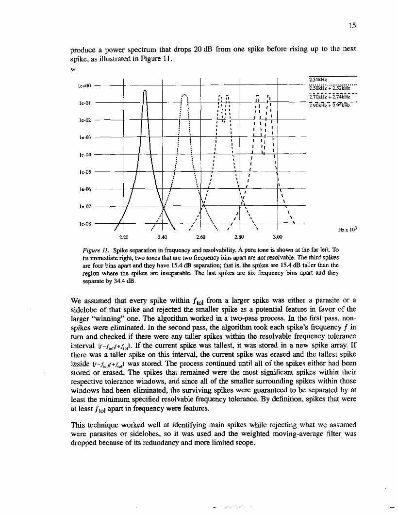
produce a power spectrum that drops 20 dB from one spike before rising up to the next spike, as illustrated in Figure 11. W

2.31kHz 2.50kHz + 2.52kHz

2.701;Hz + 2.74kHz I d 1 2.90Mz + 2.95Mz

.. . . . ... . . . .. . . . .. . . . . . .. ICcOD _ - - - _ - _ _ - - - - - - - - - _ - - - -

IC-02

le43

le-M

le-05

led6

le-07

H z x Id le08

2.20 2.40 2 . m 2.80 3.00

Figure 11. Spike separation in frequency and resolvability. A pure tone is shown at the far left To its immediate right, two tones that are two frequency bins apart are not resolvable. The third spikes are four bins apart and they have 15.4dB separation; that is, the spikes are 15.4 dB taller than the region where the spikes are inseparable. The last spikes are six frequency bins apart and they separate by 34.4 dB.

We assumed that every spike within ftol from a larger spike was either a parasite or a sidelobe of that spike and rejected the smaller spike as a potential feature in favor of the larger “winning” one. The algorithm worked in a two-pass process. In the first pass, non- spikes were eliminated. In the second pass, the algorithm took each spike’s frequency f in turn and checked if there were any taller spikes within the resolvable frequency tolerance interval W - ~ ~ , J + ~ J . If the current spike was tallest, it was stored in a new spike array. If there was a taller spike on this interval, the current spike was erased and the tallest spike inside @ - f i m , f + f , o ~ was stored. The process continued until all of the spikes either had been stored or erased. The spikes that remained were the most significant spikes within their respective tolerance windows, and since all of the smaller surrounding spikes within those windows had been eliminated, the surviving spikes were guaranteed to be separated by at least the minimum specified resolvable frequency tolerance. By definition, spikes that were at least ftOl apart in frequency were features.

This technique worked well at identifying main spikes while rejecting what we assumed were parasites or sidelobes, so it was used and the weighted moving-average filter was dropped because of its redundancy and more limited scope.

16

5.2 Prototype Definition As in Section 4.1, we needed to generate a small set of representative vectors (prototypes) for each class given the much larger set of training data. Because each test object exhibited frequency scatter, we could not use the class means as prototypes. Instead, we used cluster means. While the most significant extracted features from a given object’s trials might not all be the same (even within acceptable limits of frequency jitter), we observed that typically the features naturally separated into several distinct frequency clusters across the spectrum, so we used each cluster’s mean as one of several class prototypes. This simply meant that instead of comparing a test vector to each of five class prototypes, where the prototypes were class means, we had to compare the test vector to several prototypes for each class. In keeping with minimumdistance classifier theory, the test vector was still assigned to the same class as the prototype that yielded the lowest error. This section describes how we identified clusters and generated class prototypes from the featureextracted training data.

For all i classes with k samples in every class, N features were extracted, sorted by amplitude and tagged with ordinal feature numbers. The “first feature” was the most significant (highest-amplitude) spike in the frequency domain, the “second feature” was the second-highest, and so on. Once labeled, the features were compiled in a database of frequency-amplitude pairs for each feature number for every class, making a total of Ni databases with k elements in each. Then each database was sorted by frequency and obvious frequency clusters were identified: clusters were separated by at least fml and were taken to be about 2f,,l in scope, and single features that did not belong to any obvious cluster were ignored as anomalies. Features were separated according to frequency cluster, and the two- dimensional (frequency and amplitude) cluster means and variances were found and stored in a protoqpe file for that class’ ordinal feature.

For example, suppose 24 samples of training data are taken from the clay brick and one feature is extracted from each sample. This feature is the largest-amplitude spike in each sample’s spectrum, and these 24 “first features” would be compiled in a database. Suppose the representative frequencies in this database break down as shown in Table 2.

In this example, there are three obvious clusters (-2000 Hz, 3000 Hz and 3200 Hz) and one anomaly (3400 Hz). The single feature identified at 1980 Hz is not rejected as an anomaly, because it is within the resolvable frequency tolerance (fto, = 60 Hz) of the 2000 Hz cluster. Thus the prototype for the clay brick‘s first features contains three records, one for each cluster identified above, and each record contains the frequency mean and variance and the

17

1980

amplitude mean and variance. Note that the prototype data depends on only 23 samples, not 24, since the outlying 3400 Hz feature is ignored.

Table 2: Example of Extracted Features’ Frequency Distribution

1

Number of

that Produced Features

Identified Frequency

(Hz)

2010 6

3400

For some classes the features did not separate cleanly by at least the resolvable frequency tolerance ftol. These cases required that a clustering algorithm more sophisticated than a single cursory review be used; in this case, we used the k-means algorithm [9], whose block diagram is shown in Figure 12. Acknowledging that the k-means algorithm depends on user- defined, fixed parameters- the number of clusters and starting guesses for cluster means- and thus is not guaranteed to cluster all the data to optimize classifier performance [9], nevertheless it proved satisfactory for this problem.

We used this algorithm on the low-frequency features for the wood block. Features were spread out in frequency from about 458Hz to 976Hz. and there were no obvious boundaries to frequency clusters. We assumed there were five clusters and applied the k- means algorithm. After six iterations it stabilized and yielded the final clusters that were analyzed and stored in the appropriate prototype.

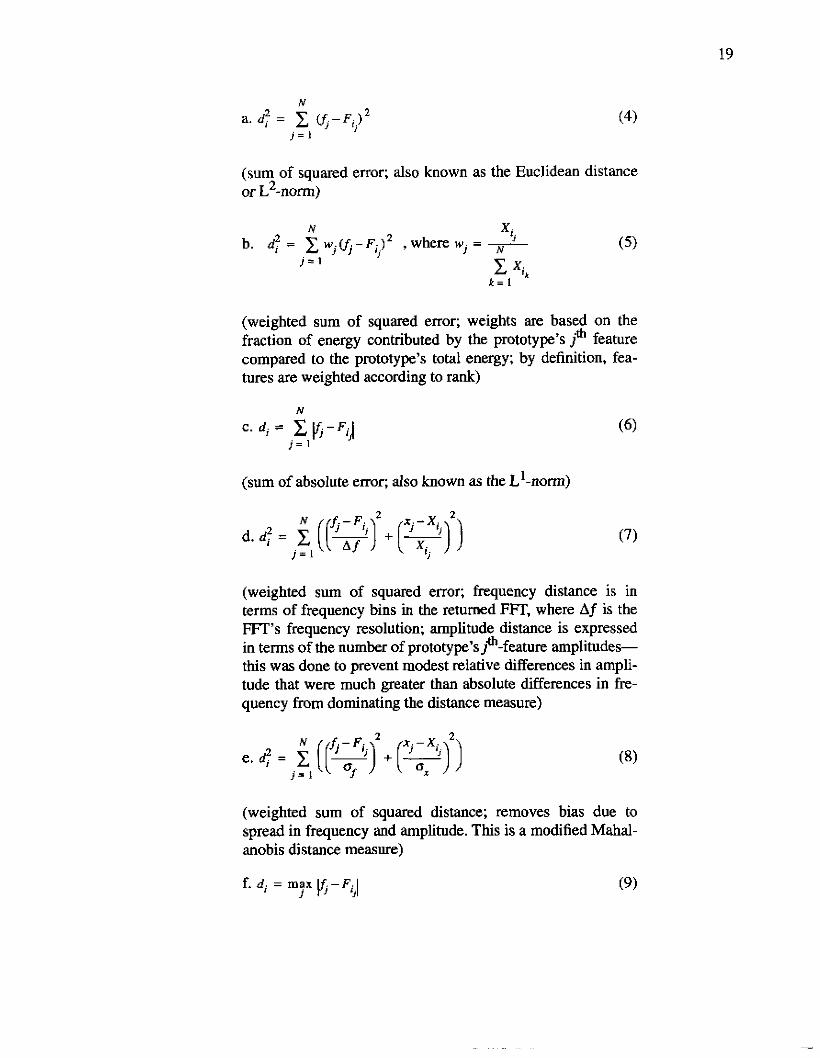
5.3 Extracted-Feature Minimum-Distance Classification We experimented with six minimum-distance classifiers on the feature-extracted data. Since we extracted only the first two features from the training and test data, the minimum- distance classifiers used two-dimensional distance measures, one dimension per feature.’ Each classifier differed only in its definition of distance, given in Equations 4 through 9.

During program execution, the classifier first read in a test sample and extracted the first two features as described in Section 5.1. Then it read the first class’ prototype file and found the

I . The number off.ml”res eithcr single-mordinate dala (fraycncy) a ordered pairs (hequency and amplimde). each of which defines a single fealu- determines the dimnsion of the Classifier. While a classifier might calculate the distance bcoveen 2-D vectors whose components were hemselves ordered pairs, ii is sal considemd a 2-D distance measure for rhe purpose of this repepoR.

18

I choose number of clusters k

cboose cluster means IhrP2. .... Pk

l or

I classify each test

vector xj

have pi’s Changed? stop

Figure 12. The k-means algorithm.

nearest-neighbor prototypes (one for each feature number) to the sample’s extractel features; these nearest neighbors were stored in a distilled prototype vector. Finally, the test sample’s feature vector and the distilled prototype were passed to an error calculator, which found the distance between the test sample’s features and the distilled prototype. The distance was stored along with the prototype’s class number and the classifier read in the next class’s database, repeating the procedure, until a minimum distance had been found for each class’ nearest-neighbor (to the test sample) prototype. The minimum of these minimum distances was taken to be the nearest neighbor to the test sample, and its associated class was taken to be the best match.

Each of the six minimumdistance classifiers used a different distance measure. The formulas used were’

I . The distances d, between a vector and class q‘s Pmtotype are given f a N Fcahues: fj is the hqwncy cowdinate of the test sample’s j” feature; F,. is the frequency d i n a t e of c;s prototype'^^^ featut: xj is the amplitude mmdinate of the test s ~ m -

ple’sj* featwe; and X i . is the amplitude wordinate of c;s prmtype’sj* featore. I

J

19

N 2 2 a. d, = ( . - F i )

I j = 1

(4)

(sum of squared error; also known as the Euclidean distance or L2-norm)

(weighted sum of squared error; weights are based on the fraction of energy contributed by the prototype's j' feature compared to the prototype's total energy; by definition, fea- tures are weighted according to rank)

N .. C. di = K - F ; J

j = l J

(sum of absolute error; also known as the L'-norm)

2 N f . - F . x . - x . d.dj)= ((%) +(-"I) xi.

j = l (7)

(weighted sum of squared error; frequency distance is in terms of frequency bins in the returned FFT, where Af is the FFT's frequency resolution; amplitude distance is expressed in terms of the number of prototype'sj&-feature amplitudes- this was done to prevent modest relative differences in ampli- tude that were much greater than absolute differences in fre- quency from dominating the distance measure)

j = l

(weighted sum of squared distance; removes bias due to spread in frequency and amplitude. This is a modified Mahal- anobis distance measure)

20

(maximum single-feature distance; also known as the L-- norm)

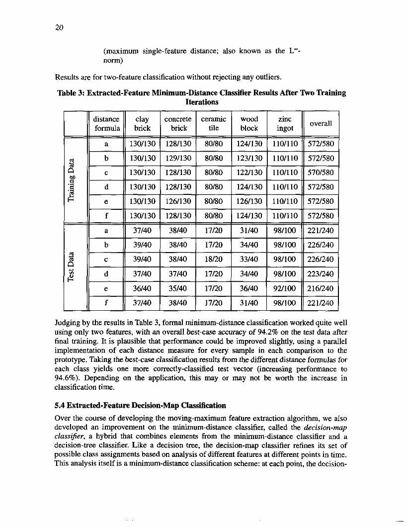
Results are for two-feature classification without rejecting any outliers.

Table 3 Extracted-Feature Minimum-Distance classifier Results After lko Training Iterations

130/130 I 128/130 I SOB0 I 124130 I 110/110 11 572/580 I I I I I I II

a \I 37/40 I 38/40 I 17/20 I 31/40 I 98/100 1) 221/240

Judging by the results in Table 3, formal minimum-distance classification worked quite well using only two features, with an overall best-case accuracy of 94.2% on the test data after final training. It is plausible that performance could be improved slightly, using a parallel implementation of each distance measure for every sample in each comparison to the prototype. Taking the best-case classification results from the different distance formulas for each class yields one more correctly-classified test vector (increasing performance to 94.6%). Depending on the application, this may or may not be worth the increase in classification time.

5.4 Extracted-Feature Decision-Map Classification Over the course of developing the moving-maximum feature extraction algorithm, we also developed an improvement on the minium-distance classifier, called the decision-map classi$er, a hybrid that combines elements from the minimum-distance classifier and a decision-tree classifier. Like a decision tree, the decision-map classifier refines its set of possible class assignments based on analysis of different features at different points in time. This analysis itself is a minimum-distance classification scheme: at each point, the decision-

-

21

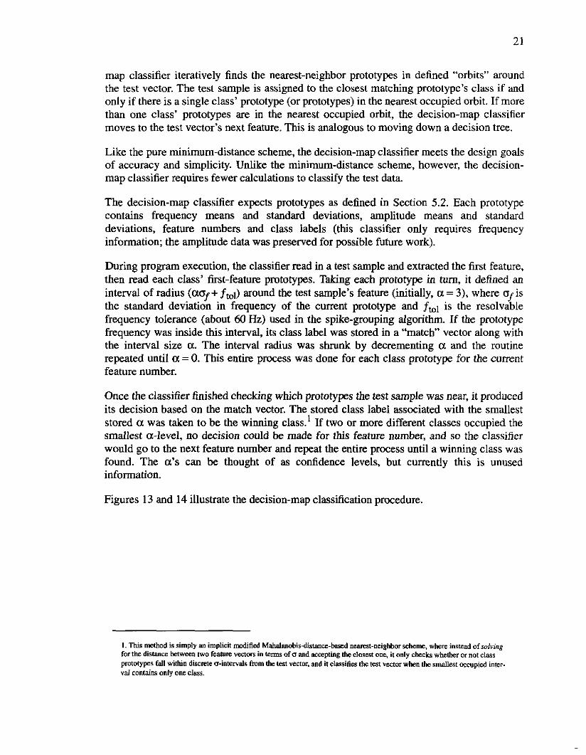
map classifier iteratively finds the nearest-neighbor prototypes in defined “orbits” around the test vector. The test sample is assigned to the closest matching prototype’s class if and only if there is a single class’ prototype (or prototypes) in the nearest occupied orbit. If more than one class’ prototypes are in the nearest occupied orbit, the decision-map classifier moves to the test vector’s next feature. This is analogous to moving down a decision tree.

Like the pure minimum-distance scheme, the decision-map classifier meets the design goals of accuracy and simplicity. Unlike the minimum-distance scheme, however, the decision- map classifier requires fewer calculations to classify the test data.

The decision-map classifier expects prototypes as defined in Section 5.2. Each prototype contains frequency means and standard deviations, amplitude means and standard deviations, feature numbers and class labels (this classifier only requires frequency information; the amplitude data was preserved for possible future work).

During program execution, the classifier read in a test sample and extracted the first feature, then read each class’ first-feature prototypes. Taking each prototype in turn, it defined an interval of radius (aaf+ ft,l) around the test sample’s feature (initially, a = 3), where of is the standard deviation in frequency of the current prototype and fml is the resolvable frequency tolerance (about 60 Hz) used in the spike-grouping algorithm. If the prototype frequency was inside this interval, its class label was stored in a “match” vector along with the interval size a. The interval radius was shrunk by decrementing a and the routine repeated until a = 0. This en& process was done for each class prototype for the current feature number.

Once the classifier finished checking which prototypes the test sample was near, it produced its decision based on the match vector. The stored class label associated with the smallest stored a was taken to be the winning class.’ If two or more different classes occupied the smallest a-level, no decision could be made for this feature number, and so the classifier would go to the next feature number and repeat the entire process until a winning class was found. The a’s can be thought of as confidence levels, but currently this is unused information.

Figures 13 and 14 illustrate the decision-map classification procedure.

I T h ~ s nlechod ip rirnpl) an implicil mcdficd M ~ d a n o b i ~ d i b m c e - b d nrmt-neighbor &mr. ukrr inwad of re/.mp for thc dislanur &ween 1-0 feature wxm in Vrm~ ofa and accepting lhe c l m c ~ one. i t only checks whether or no! cl.1~1 prototypes fall uitluo dtscme a-inunak fmm the cest vector. and it classilia the 1 6 1 vector when Ihc sc~Lllles1 occup~cd mer. val conwum only onc class.

22

power 1

++++I frequency a 3 203 -

202 0 2

Figure 13. Example of decision-map classification using the first feature. Class A (denoted by solid gray arrows) has a single first-feature prototype and class B (bollow gray arrows) has two. The test vector (solid black armw) is inside the a = 1 interval to both class A's prototype (spike 1) and one of class B's prototypes (spike 2). Since the test vector is equidistant (in a) to both class' prototypes, classification is not possible using this feature.

power

Test

- frequency 204 0 4 I 4

I

2% D5

Figure 14. Decision-map classification using the second feature. As classification was not possible using the first feature in Figure 13, the decision-map uses the next f e a m . Class A is denoted by solid gray arrows and has one second-feature prototype; class B is denoted by hollow gray mows and also has one second-feature prototype. The test vector's second feature (solid black arrow) is inside the a = 2 interval to class A's prototype (spike 4) and is inside the a = 1 interval to class B s prototype (spike 5 ) . Since the test veztor is closer in a to class B s prototype, the test sample is assigned to class B.

23

Table 4 shows the classifier's results.

Table 4: Decision-Map Classifier Results After ' b o a a i n h g Iterations

The decision-map classifier worked as well as the minimum-distance classifier, with an overall accuracy of 93.8% on the extracted-feature test data. Even though it was implicitly based on a Mahalanobis distance measure, the decision map misclassified fewer samples than the formal Mahalanobis minimum-distance classifier did, performing as well as the best formal minimum-distance classifier, which was based on the L'-norm.

Certain details could be modified to potentially improve performance. One of these is, naturally, the expansion of prototypes to higher feature numbers. Another reasonable improvement would be to optimize the interval size around the current feature when identifying the prototypes closest to it. Currently, this interval takes on only three discrete values that depend on a variable datum for each prototype, namely, of. If this variable were optimized for all prototrpes based on the training data, there might be some slight improvement in classification. Both of these changes would occur before the classifier ran, so execution time compared to the nearest neighbor's would not change for the worse.

5.5 Comparisons Both kinds of extracted-feature classifiers outperformed the full-spectrum minimum- distance classifier, so this section compares the two with each other. As there was no significant difference in classifier performance, the choice of one method over another rests on secondary specifications. One such specification is computational complexity. The minimum-distance approach had to evaluate its distance function once for every cluster mean stored in each prototype file (recall that the class prototypes stored all cluster means per feature number and the classifier determined which feature number's cluster mean to use). Assume each class ci has Nil first-feature clusters, Ni2 second-feature clusters, and so on to N ~ K clusters at the fl-feature level. TO select the closest cluster within class cis

prototype to the test sample, the distance equation must be evaluated N, times. This is

only to select the nearest cluster mean for this particular class; to find the appropriate cluster

means for all P classes requires x ( N.. ,,] evaluations. Finally, P more K-feature evaluations

are required to perform the actual classification, for a total of

K

i = 1

P Kt

i=, j = ,

24

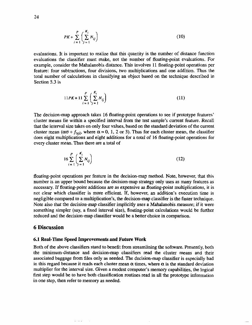
PK+ (2 N i j ) i = l j = l

evaluations. It is important to realize that this quantity is the number of distance function evaluations the classifier must make, not the number of floating-point evaluations. For example, consider the Mahalanobis distance. This involves 11 floating-point operations per feature: four subtractions, four divisions, two multiplications and one addition. Thus the total number of calculations in classifying an object based on the technique described in Section 5.3 is

The decision-map approach takes 16 floating-point operations to see if prototype features’ cluster means lie within a specified interval from the test sample’s current feature. Recall that the interval size takes on only four values, based on the standard deviation of the current cluster mean (no + fml, where a = 0, 1, 2 or 3). Thus for each cluster mean, the classifier does eight multiplications and eight additions for a total of 16 floating-point operations for every cluster mean. Thus there are a total of

floating-point operations per feature in the decision-map method. Note, however, that this number is an upper bound because the decision-map strategy only uses as many features as necessary. If floating-point additions are as expensive as floating-point multiplications. it is not clear which classifier is more efficient. If, however, an addition’s execution time is negligible compared to a multiplication’s, the decision-map classifier is the faster technique. Note also that the decision-map classifier implicitly uses a Mahalanobis measure; if it were something simpler (say, a fixed interval size), floating-point calculations would be further reduced and the decision-map classifier would be a better choice in comparison.

6 Discussion

6.1 Real-Time Speed Improvements and Future Work Both of the above classifiers stand to benefit from streamlining the software. Presently, both the minimum-distance and decision-map classifiers read the cluster means and their associated baggage from files only as needed. The decision-map classifier is especially had in this regard because it reads each cluster mean a times, where a is the standard deviation multiplier for the interval size. Given a modest computer’s memory capabilities, the logical first step would be to have both classification routines read in all the prototype information in one step, then refer to memory as needed.

25

The other immediate improvement would be to trade speed for functionality. Currently the classifier is at a functional point between a complete “black box” system and a basic classifier. In its complete form, the black box would accept raw time-amplitude data and take care of all preprocessing internally before classifying. The basic classifier, on the other hand, expects reduced feature vectors that were produced from external preprocessing steps. Right now the system accepts the full-spectrum array for each sample, extracts the features and then passes the feature vector to the classifier module. Both the minimum-distance and decision-map classifier systems work this way, and each classifies an object in roughly two seconds.

Based on the results of the classifier trials, two-dimensional minimum-distance schemes deserve another chance. Because the problem that dogged 2-D classification was amplitude spread, elementary amplitude transformations (e.g. logarithms) should provide tighter clustering in that dimension, and we hope to see results comparable to the I-D version explored here.

We would also like to determine how the spectra of the test objects varies with force. If different force magnitudes excite different frequency components in each object, this would establish a larger base of information to search for appropriate features. Hopefully, this would improve classification by providing additional significant features (such as force knowledge) for test samples that otherwise cannot be classified with the current extracted- feature minimum-distance and decision-map schemes.

6.2 Summary

We are interested in the problem of classifying objects based on their acoustic emissions when physically struck. To this end we sampled five different objects: a clay brick, a concrete brick, a ceramic tile, a wooden block and a zinc ingot. Dropping a cane onto each, we hit the objects at various locations on their surfaces, and sampled and stored the resulting sound of impact. As previous work has shown that spectral elements of acoustic signals are sufficient for certain classification schemes, we used spikes in the frequency domain as classifier features.

A fundamental design goal of this project was simplicity, but one of the simplest pattern recognition techniques- a minimum-distance classifier that used entire spectra as input vectors- could not classify four of the five classes. We assumed this was due to joint effects of intraclass variation, large-valued spikes and the large size of the input vectors, so we developed a moving-maximum window to extract the N largest spikes in the frequency domain and used these spikes as feature vectors. After identifying clusters of each class’ representative frequencies, we created class prototypes, vectors whose elements were the cluster means of the training data’s extracted features. We then passed the prototypes and test samples’ extracted-feature data to two kinds of classifiers, the minimum-distance classifier and the decision-map classifier.

The minimum-distance classifier calculated the error between a test vector and each prototype using every vector element (feature), and assigned the test sample to the prototype that yielded the lowest error measure. The decision-map classifier, a variant on the standard

26

minimum-distance classifier, iteratively found the nearest prototype vector to the test sample based on each vector’s most significant feature. If a single best match was found, the test vector was assigned to the same class. Otherwise, the classifier repeated the process using additional features as necessary.

While the decision-map classifier performed as well on feature-extracted data as the minimum-distance classifier, with 94% accuracy, it has a computational advantage. The minimum-distance classifier calculates its distance measure a fixed number of times that is a function of the number of features. The decision-map classifier, on the other hand, uses only as many features as necessary, so it often does significantly fewer calculations than the minimum-distance classifier does.

6.3 Conclusion In order to function autonomously, robots must have some way of extracting information from their surroundings and then applying that information to perform specific tasks. Specifically, the ability to do classification given raw data is an important step towards machine intelligence. We address the problem of sound-based object classification and speculate that the establishment of a knowledge base of many different objects’ acoustic properties can provide clues to help robots infer general material properties about its environment from acoustic tests. This paper provides a necessary starting point for this area of research.

7 Acknowledgments This report was originally written as a project thesis, in partial fulfillment of the requirements for the Master of Science degree in the department of Electrical and Computer Engineering at Cmegie Mellon University. The following people were especially helpful in support of that work.

Foremost, I am indebted to Professor Eric P. Krotkov for many months of encouragement, criticism, guidance and support. Without his help I would have foundered long ago. I also gratefully acknowledge Professor Take0 h a d e for his many helpful comments and suggestions.

I wish to thank Professor Robert T. Schumacher, for explaining problems inherent in the analysis of vibrating rigid bodies and providing additional sources for analyzing shape from acoustics. Also, I appreciate Professor Richard M. Stern’s and Melvin W. Siegel’s graciously lending specialized test equipment.

Finally, I thank Dr. Erik K. Witt for all his help with coding, signal processing and pattern recognition concepts.

27

8 References [l] Stewart, Clayton, et al. “Classification of Atmospheric Acoustic Signals from Fixed-

Wing Aircraft,” Signal Processing, Sensor Fusion and Target Recognition (SPIE Proceedings), vol. 1699, pp. 136-43, 1992.

[2] Legitimus, D. and Schwab, L. “Experimental Comparison between Neural Networks and Classical Techniques of Classification Applied to Natural Underwater Transients Identification,” IEEE Conference on Neural Networks for Ocean Engineering, pp. 113-120, 1991.

[3] Beck, Steven, et al. “A Hybrid Neural Network Classifier of Short Duration Acoustic Signals,” International Joint Conference on Neural Networks, vol. 1, pp. 119-24, 1991.

[4] Stewart, C. and Larson, V. “Detection and Classification of Acoustic Signals from Fixed-Wing Aircraft,” IEEE International Conference on Systems Engineering, pp. 25-8, 1991.

[5] Perron, Marie-Claude. “Feature Extraction and Learning Decision Rules from Ultrasonic Signals; Applicability in Non-Destructive Testing,” ZEEE 1988 Ultrasonics Symposium Proceedings, vol. 1, pp, 533-6, 1988.

[6] Oppenheim, Alan V. and Schafer, Ronald W. Discrete-Time Signal Processing. Englewood C l i s , NJ: Prentice Hall, 1989.

[7] Kac, Mark. “Can One Hear the Shape of a Drum?” American Mathematical Monthly, vol. 73, number 4, part Il, pp. 1-23,1966.

[8] Fisher, Michael E. “On Hearing the Shape of a Drum,” Journal of Combinarorial %OV, VOI. 1, pp. 105-125, 1966,

[9] Duda, Richard 0. and Hart, Peter E. Patfern Classijcation and Scene Analysis. New York John Wiley and Sons, 1973.

Appendix A- Test Objects' Average Spectra

Linear Scale w 10-3

4.00

3.50

3.00

2.50

2 . 0

1 .so I .00

0.50

0.00

W

1e03

1e-04

1e05

1c-06

1c-07 i 1c08

Semilog Scale

A- 1

10.00 0.m 5.00 10.00 0.00 5.00

Figure A-1. Clay brick's average spectrum, taken over 30 trials.

Linear Scale w i 10-6 W

HZ x 103

1ed3

1e44

1c05

1c-06

1d7

1e-08

1e-09

1c-10

Semilog Scale

0.00 5.00 1o.m 0.0 5.03 10.00

Figure A-2. Concrete brick's average spectrum, taken over 30 trials.

A-2

Linear Scale wY.106

600.00

400.00

W

le-03

led4

l e45

le-06

l d l

le-OS

Semilog Scale

t I

wx 104

30.00

25.w

20.w

15.00

10.00

5.00

0.00

Linear Scale W

- I I I

I I H r x I d 5.00 10.00 0.00 5.00 10.00 0.00

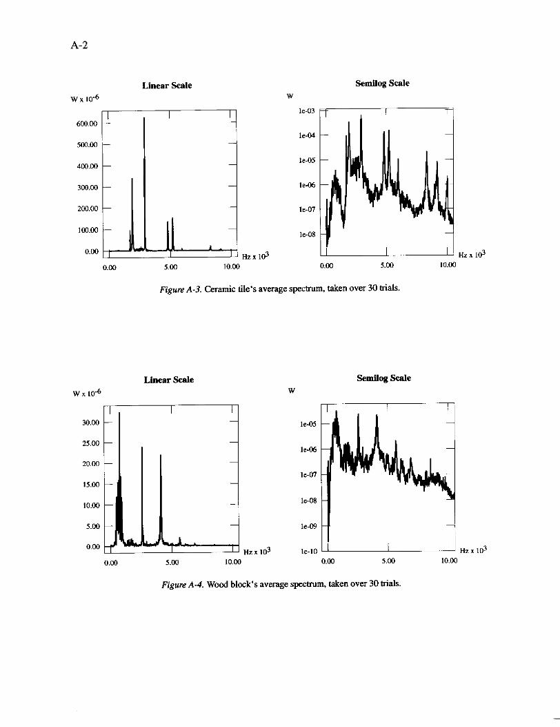
Figure A-3. Ceramic tile's average spectrum, taken over 30 trials.

Hzrld

led6

le-W

le-os

1 4 9

le-10 0.00 5.W 10.00 000 5.00 10.00

Figure A-4. Wood block's average spectrum, taken over 30 bids.

A-3

I I I 1.60 -

1.40 -

1.20 -

1.00 -

-

-

-

-

0.80 - -

0.60 - -

0.40 - 4

0.20 -

0.0 - i 1 Ii I Hzxld

Semilog Scale W

le43 ' I I

k-04

l e 4 5

IS46

IC-W

IC-08

1s-IO = I0.W HZXl 0.0 5.00

Figure A-5. Zinc ingot's average spectrum, taken over 30 bials.

Appendix B- Sequence of Signal Processing B-1

Raw Time Data

v 10-3

40.00

30.00

20.00

10.00

0.00

-10.00

-20.00

-30.00

-40.00 s x 10-3 0.00 20.00 40.00 60.00 80.00 100.00

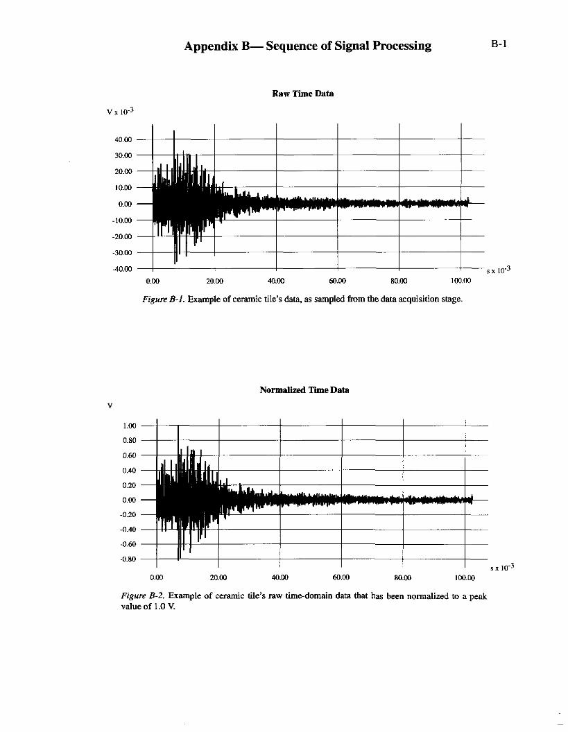
Figure B-1. Example of ceramic tile’s data, as sampled from the data acquisition stage.

Normalized T i e Data

v

1 .00

0.80

0.60

0.40

0.20

0.00

-020

-0.40

-0.60

-0.80 I

I 10-3 0.00 20.00 40.00 m.00 80.00 1OO.M

Figure B-2. Example of ceramic tile’s raw timedomain data tbat has been normalized to a peak value of 1 .O V.

B-2

_. -L -_.-. ~~ -A ~~ ~

J

Frequency Power Spectrum

H Z X 103

w x 10-6

120.00

100.00

80.00

60.00

40.00

20.00

0.00 3 H~ 103 0.00 2.00 4.00 6.00 8.00 10.00 12.00

Figure 8-3. Example of ceramic tile’s frequency-domain data. The power spectrum was obtained by taking the W p o i n t FFT of the normalized data (shown in Figure B-2).

Spike Extraction

w x 10-6

120.00

100.00

80.00

60.00

20.00

0.00 c I --.--

B-3

w x 10-6

120.w

60.00

4o.w ‘T 20.00

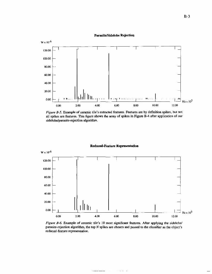
Parasite/Sidelobe Rejection

I I I I

0.00 2.00 4.00 6.00 8.00 10.00 12.00

Figure B-5. Example of ceramic tile’s extracted features. Features are by definition spikes, but not all spikes are features. This figure shows lhe m y of spikes in Figure B-4 after application of our sidelobe/parasitere.jection algorithm.

w x 10-6

120.w

80.00

40.00 60.00 L I I I I I I ,

0.00 2.00 4.00 6.00 8.00 10.00 12.00

Figure 8-6. Example of ceramic tile’s 10 most significaot features. After applying the sidelobe/ parasite-rejection algorithm, the top N spikes are chosen and passed to the classifier as the object’s reduced-feature representation.