OBBTree: A Hierarchical Structure for

Rapid Interference Detection

Gottschalk, M. C. Lin and D. Manocha

Department of Computer Science, University of N.

Carolina, Chapel Hill.

Presenter: Tao Ju

Spring, 2001

Introduction

OBBTree: A tight-fitting hierarchical structure and an efficient overlap-testing algorithm for interference detection amongst complex models undergoing rigid motion.

 

Bounding Volume: OBB (Oriented Bounding Box)

Overlap test algorithm for OBBs: Separating Axis Algorithm

Computing Tight Fitting OBB O(n Log(n))

Triangulate polygons. ( O(n) )

Compute the convex hull of the vertices of the triangles. ( O(n Log(n)) )

Orientation of OBB: Covariance Matrix. ( O(n) )

Position and dimension of OBB. ( O(n) )

Compute Orientation of OBB

Let the i’th triangle of the convex hull have vertices pi, qi, and ri. Let the number of triangles in the convex hull be n.

The area of i’th triangle is denoted as Ai,

Ai = | (pi － qi) × (pi － ri) | / 2

The surface area of the convex hull is denoted as AH,

AH = ∑i Ai

Compute Orientation of OBB

The centroid of the i’th triangle is denoted by vector mi,

mi = ( pi + qi + ri ) / 3

The centroid of the entire convex hull is a weighted mean of the triangle centroids, denoted by mH,

mH = ∑i Aimi / AH

Compute Orientation of OBB

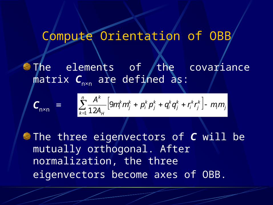
The elements of the covariance matrix Cn×n

are defined as:

Cn×n =

The three eigenvectors of C will be mutually orthogonal. After normalization, the three eigenvectors become axes of OBB.

ji

n

k

kj

ki

kj

ki

kj

ki

kj

ki

H

k

mmrrqqppmmA

A

1

912

Compute Dimension of OBB

Find the maximum and minimum extents of the original triangle set along each axis, and size the OBB.

Computing Tight Fitting OBB

Why using covariance matrix?

Second order statistics summarizing the data points.

Why using convex hull?

Avoid arbitrary influences from interior vertices of the model.

Why computing areas?

Infinitely dense sampling.

Constructing a hierarchical

OBBTree: Top-down Approach Subdivision method: Split the longest axis of an OBB with a plane orthogonal to one of its axes, partitioning the polygons according to which side of the plane their center point lies on.

The subdivision coordinate along that axis was then chosen to be that of the mean point of the vertices.

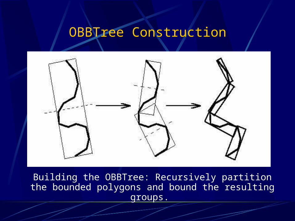
OBBTree Construction

Building the OBBTree: Recursively partition the bounded polygons and bound the resulting groups.

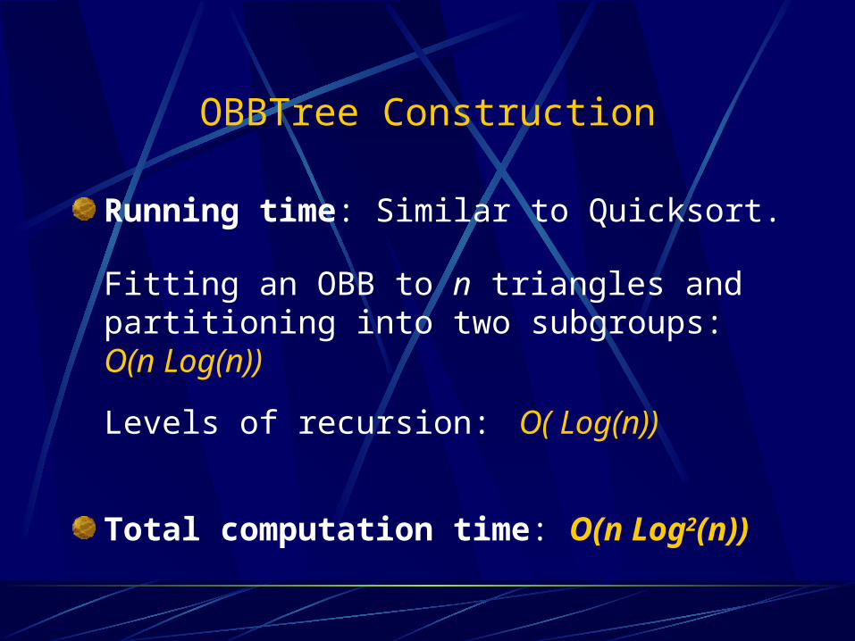
OBBTree Construction

Running time: Similar to Quicksort.

Fitting an OBB to n triangles and partitioning into two subgroups: O(n Log(n))

Levels of recursion: O( Log(n))

Total computation time: O(n Log2(n))

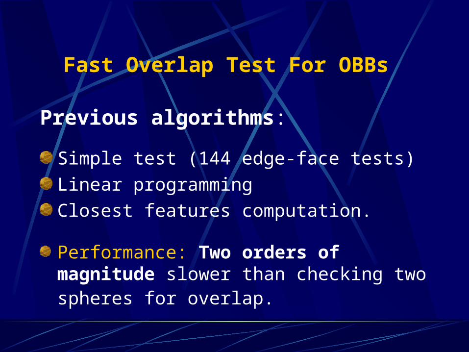
Fast Overlap Test For OBBs

Previous algorithms:

Simple test (144 edge-face tests)

Linear programming

Closest features computation.

Performance: Two orders of magnitude slower than checking two spheres for overlap.

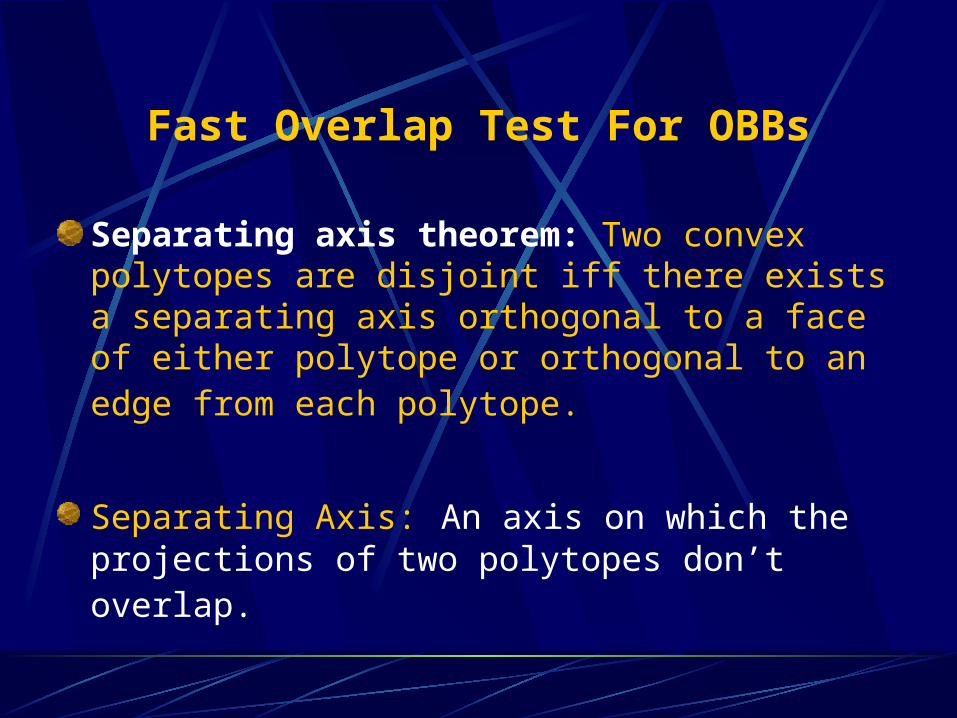
Fast Overlap Test For OBBs

Separating axis theorem: Two convex polytopes are disjoint iff there exists a separating axis orthogonal to a face of either polytope or orthogonal to an edge from each polytope.

Separating Axis: An axis on which the projections of two polytopes don’t overlap.

Fast Overlap Test For OBBs

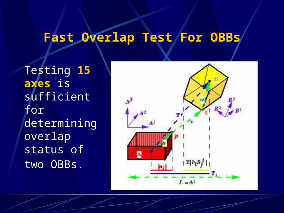
Testing 15 axes is sufficient for determining overlap status of two OBBs.

Fast Overlap Test For OBBs

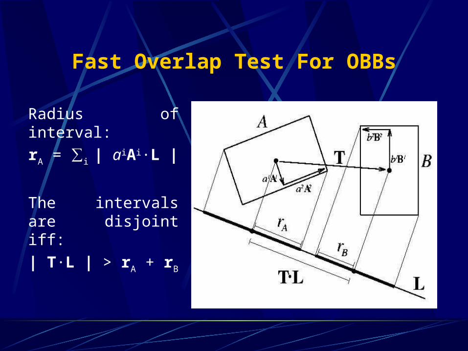
Radius of interval:

rA = ∑i | aiAi·L |

The intervals are disjoint iff:

| T·L | > rA + rB

Fast Overlap Test For OBBs

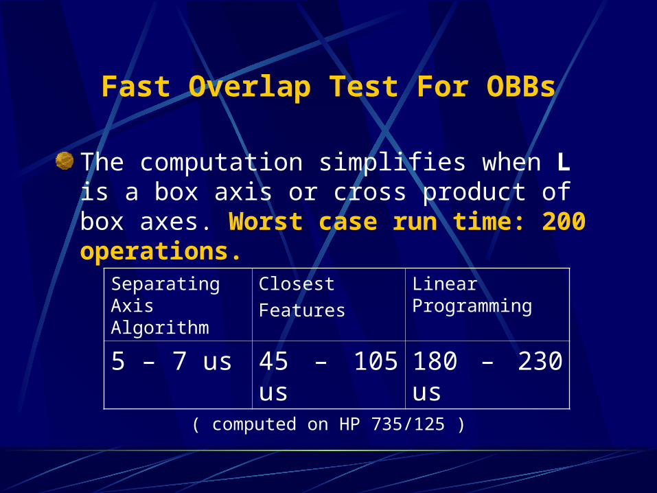
The computation simplifies when L is a box axis or cross product of box axes. Worst case run time: 200 operations.

( computed on HP 735/125 )

Separating Axis Algorithm

Closest

Features

Linear Programming

5 – 7 us 45 – 105 us 180 – 230 us

Comparison Of Bounding Volumes

Bounding volumes:

Spheres AABBs ( Axis Aligned Bounding Boxes ) OBBs ( Oriented Bounding Boxes )

Comparison Of Bounding Volumes

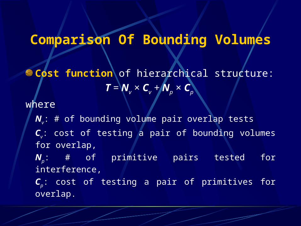
Cost function of hierarchical structure:

T = Nv × Cv + Np × Cp

where

Nv: # of bounding volume pair overlap tests

Cv: cost of testing a pair of bounding volumes for overlap,Np: # of primitive pairs tested for interference,

Cp: cost of testing a pair of primitives for overlap.

Comparison Of Bounding Volumes

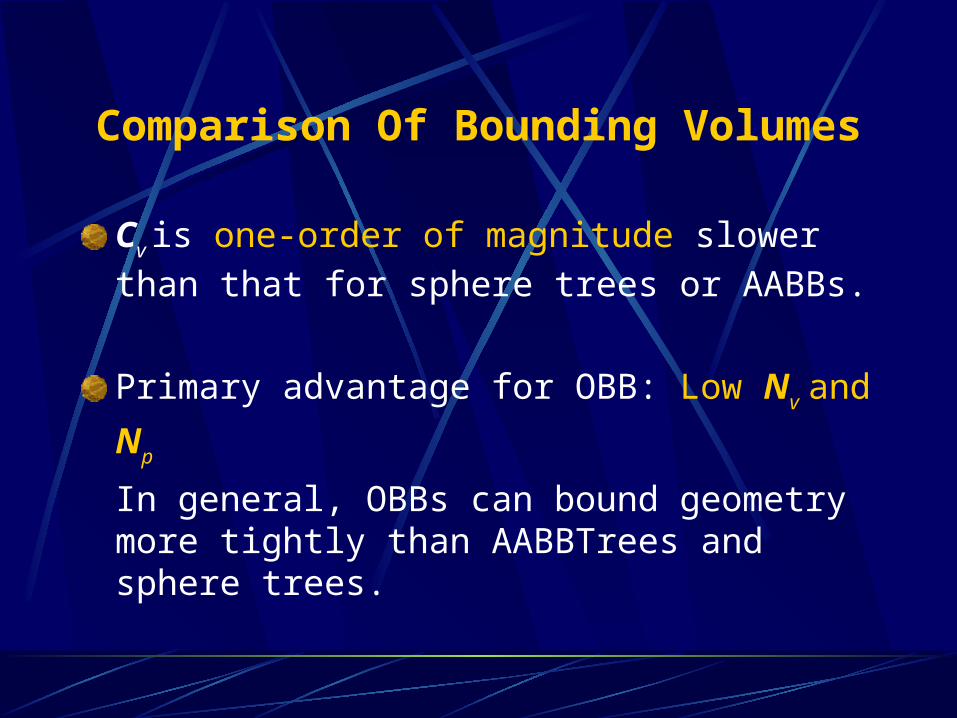
Cv is one-order of magnitude slower than that

for sphere trees or AABBs.

Primary advantage for OBB: Low Nv and Np

In general, OBBs can bound geometry more tightly than AABBTrees and sphere trees.

Comparison Of Bounding Volumes

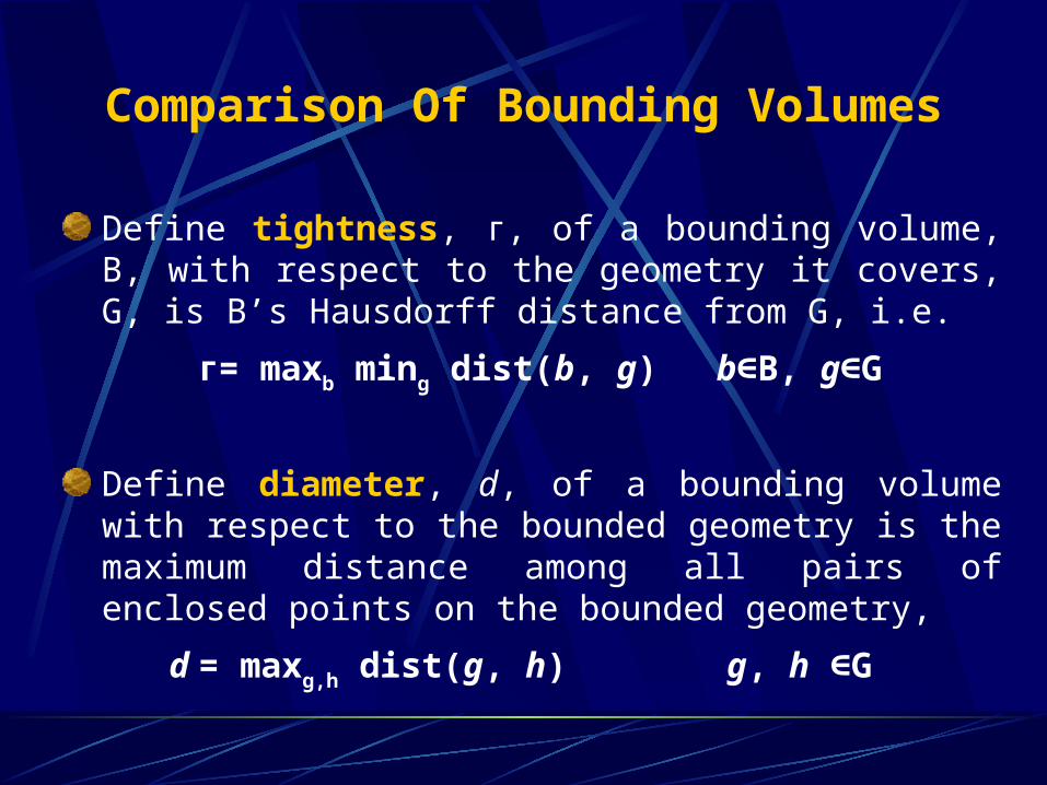
Define tightness, г, of a bounding volume, B, with respect to the geometry it covers, G, is B’s Hausdorff distance from G, i.e.

г= maxb ming dist(b, g) b∈B, g∈G

Define diameter, d, of a bounding volume with respect to the bounded geometry is the maximum distance among all pairs of enclosed points on the bounded geometry,

d = maxg,h dist(g, h) g, h ∈G

Comparison Of Bounding Volumes

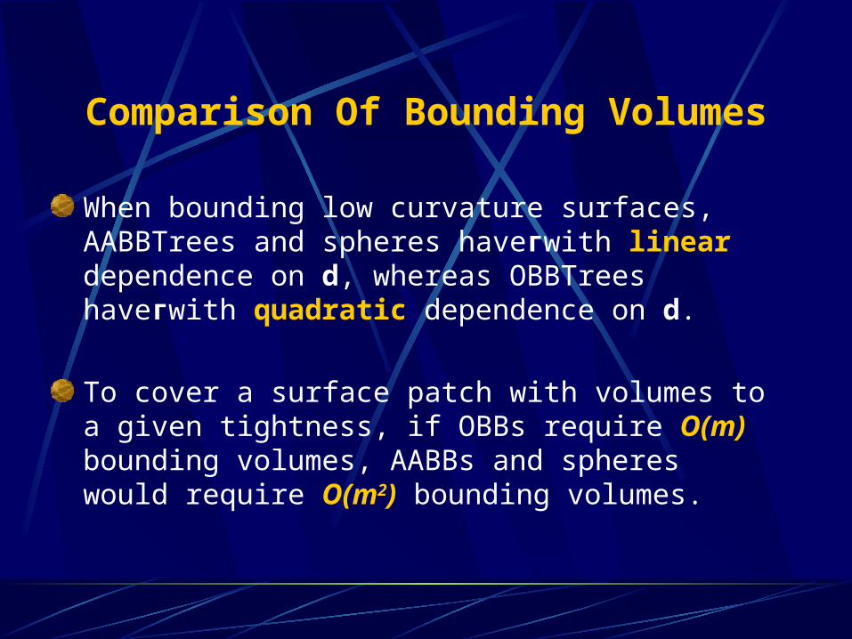
When bounding low curvature surfaces, AABBTrees and spheres haveгwith linear dependence on d, whereas OBBTrees haveгwith quadratic dependence on d.

To cover a surface patch with volumes to a given tightness, if OBBs require O(m) bounding volumes, AABBs and spheres would require O(m2) bounding volumes.

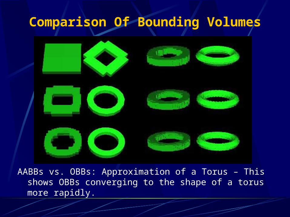
Comparison Of Bounding Volumes

AABBs vs. OBBs: Approximation of a Torus – This shows OBBs converging to the shape of a torus more rapidly.

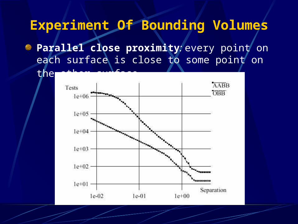
Experiment Of Bounding Volumes

Parallel close proximity: every point on each surface is close to some point on the other surface.

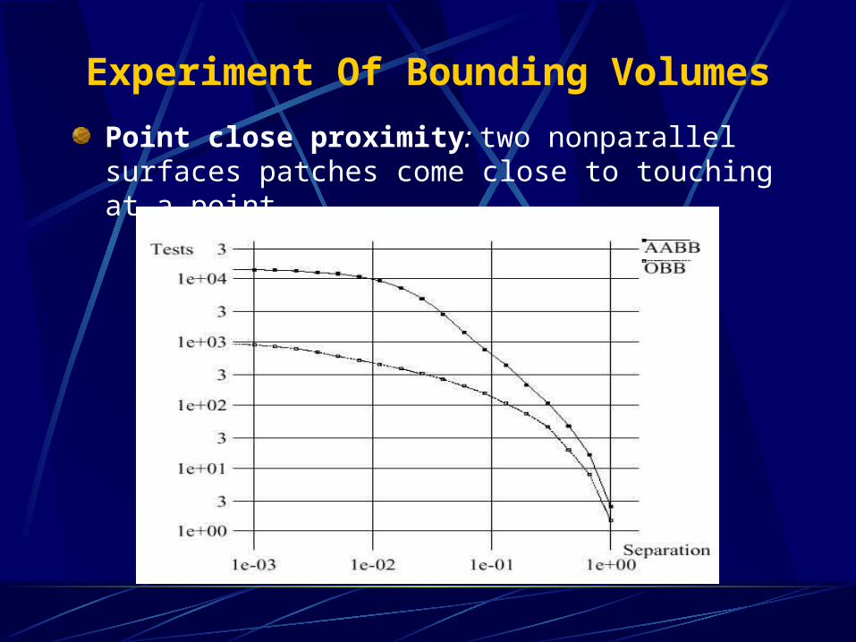
Experiment Of Bounding Volumes

Point close proximity: two nonparallel surfaces patches come close to touching at a point.

Comparison Of Performance

With AABBs: Improvement from 1/7 – 1/5 of a second for computation of all contacts between models to 1/75 – 1/25 of a second. ( on SGI Indigo2

Extreme ).

With spheres: Improvement of one order of

magnitude.

Interference Detection In Action

RAPID

V-COLLIDE

H-COLLIDE

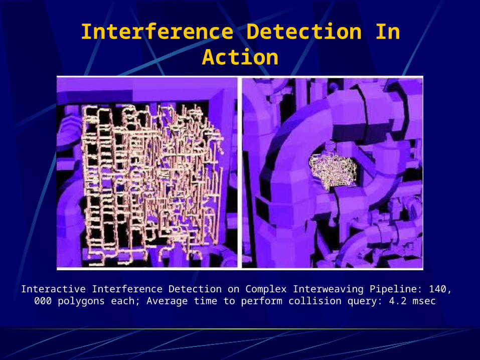
Interference Detection In Action

Interactive Interference Detection on Complex Interweaving Pipeline: 140, 000 polygons each; Average time to perform collision query: 4.2 msec

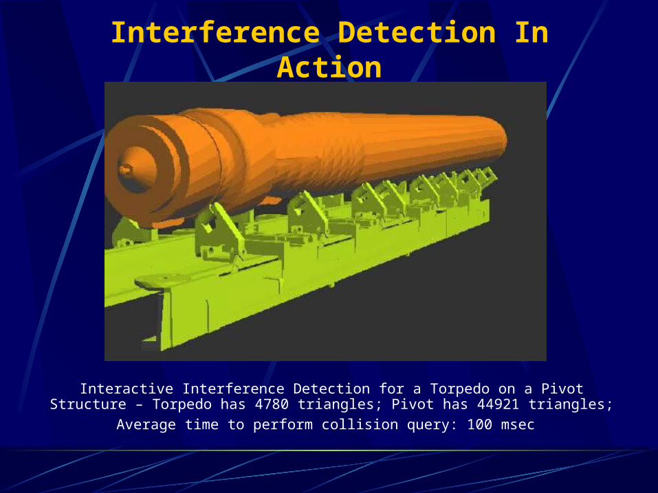
Interference Detection In Action

Interactive Interference Detection for a Torpedo on a Pivot Structure – Torpedo has 4780 triangles; Pivot has 44921 triangles; Average time to perform collision query: 100

msec

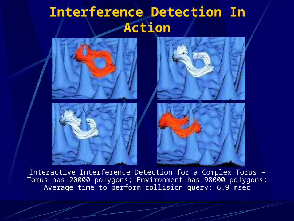
Interference Detection In Action

Interactive Interference Detection for a Complex Torus – Torus has 20000 polygons; Environment has 98000 polygons; Average time

to perform collision query: 6.9 msec

Conclusion

New efficient algorithms for hierarchical representation using tight-fitting OBBs.

Use of a “separating axis” theorem to check two OBBs for overlap in about 100 operations on average.

By comparison with AABBs, show that for many close proximity situations, OBBs are asymptotically much faster.