O-Snap: Optimization-Based Snapping for Modeling …

O-Snap: Optimization-Based Snapping forModeling ArchitectureMURAT ARIKANVienna University of TechnologyMICHAEL SCHWARZLERVRVis Research CenterSIMON FLORY and MICHAEL WIMMERVienna University of TechnologyandSTEFAN MAIERHOFERVRVis Research Center

In this paper, we introduce a novel reconstruction and modeling pipelineto create polygonal models from unstructured point clouds. We propose anautomatic polygonal reconstruction that can then be interactively refined bythe user. An initial model is automatically created by extracting a set ofRANSAC-based locally fitted planar primitives along with their boundarypolygons, and then searching for local adjacency relations among parts ofthe polygons. The extracted set of adjacency relations is enforced to snappolygon elements together, while simultaneously fitting to the input pointcloud and ensuring the planarity of the polygons. This optimization-basedsnapping algorithm may also be interleaved with user interaction. This al-lows the user to sketch modifications with coarse and loose 2D strokes, asthe exact alignment of the polygons is automatically performed by the snap-ping. The generated models are coarse, offer simple editing possibilities bydesign and are suitable for interactive 3D applications like games, virtualenvironments etc. The main innovation in our approach lies in the tightcoupling between interactive input and automatic optimization, as well asin an algorithm that robustly discovers the set of adjacency relations.

Categories and Subject Descriptors: I.3.5 [Computer Graphics]: Com-putational Geometry and Object Modeling—Geometric algorithms, lan-

Authors’ addresses: M. Arikan, Vienna University of Technology, Instituteof Computer Graphics and Algorithms, Favoritenstrasse 9-11/E186, A-1040Vienna, Austria; email: [email protected]; M. Schwarzler, VRVisResearch Center, Donau-City-Strasse 1, A-1220 Vienna, Austria; S. Flory,Vienna University of Technology, Vienna, Austria; M. Wimmer, ViennaUniversity of Technology, Institute of Computer Graphics and Algorithms,Favoritenstrasse 9-11/E186, A-1040 Vienna, Austria; S. Maierhofer, VRVisResearch Center, Donau-City-Strasse 1, A-1220 Vienna, Austria.Permission to make digital or hard copies of part or all of this work forpersonal or classroom use is granted without fee provided that copies arenot made or distributed for profit or commercial advantage and that copiesshow this notice on the first page or initial screen of a display along withthe full citation. Copyrights for components of this work owned by othersthan ACM must be honored. Abstracting with credit is permitted. To copyotherwise, to republish, to post on servers, to redistribute to lists, or to useany component of this work in other works requires prior specific permis-sion and/or a fee. Permissions may be requested from Publications Dept.,ACM, Inc., 2 Penn Plaza, Suite 701, New York, NY 10121-0701 USA, fax+1 (212) 869-0481, or [email protected]© YYYY ACM 0730-0301/YYYY/12-ARTXXX $10.00

DOI 10.1145/XXXXXXX.YYYYYYYhttp://doi.acm.org/10.1145/XXXXXXX.YYYYYYY

guages, and systems; I.3.5 [Computer Graphics]: Computational Geome-try and Object Modeling—Modeling packages

General Terms: Algorithms

Additional Key Words and Phrases: surface reconstruction, geometric opti-mization, interactive modeling

ACM Reference Format:Arikan, M., Schwarzler, M., Flory, S., Wimmer, M., and Maierhofer, S.YYYY. O-Snap: Optimization-based snapping for modeling architecture.ACM Trans. Graph. VV, N, Article XXX (Month YYYY), 15 pages.DOI = 10.1145/XXXXXXX.YYYYYYYhttp://doi.acm.org/10.1145/XXXXXXX.YYYYYYY

1. INTRODUCTION

Modeling and reconstruction of buildings poses a challenge forboth current research efforts as well as industrial applications.While data acquisition processes and techniques have experiencedenormous advances over the last years, the ensuing processing andmodeling steps are by far not as sophisticated and unproblematicto handle. Reasons for this are on the one hand the large size andnoisiness of the point cloud data gathered from laser scans, pho-togrammetric approaches or stereo cameras, and on the other handthe absence of suitable modeling tools and techniques that can han-dle the complexity of large 3D point clouds.

Converting raw input data into 3D models suitable for applica-tions like games, GIS systems, simulations, and virtual environ-ments therefore remains a complex and time-consuming task suit-able for skilled 3D artists only. Modeling applications like GoogleSketchUp and its Pointools plugin [2011] address this issue byproposing simplified user interfaces and interoperability with otherproducts like Street View (from where the artist can for exampleretrieve photogrammetric data). However, the modeling process re-mains cumbersome and time-consuming, as the accuracy of the re-construction depends on the skills and patience of the user. In con-trast, our system automatically maintains the fitting to the inputpoint cloud during the whole reconstruction and modeling process.Fully automatic reconstruction approaches may omit any user inter-action, but can hardly deliver satisfying results in case of erroneousand/or partly missing data. We overcome these limitations by let-ting a user guide the geometry completion. Although our system is

ACM Transactions on Graphics, Vol. VV, No. N, Article XXX, Publication date: Month YYYY.

2 • Arikan et al.

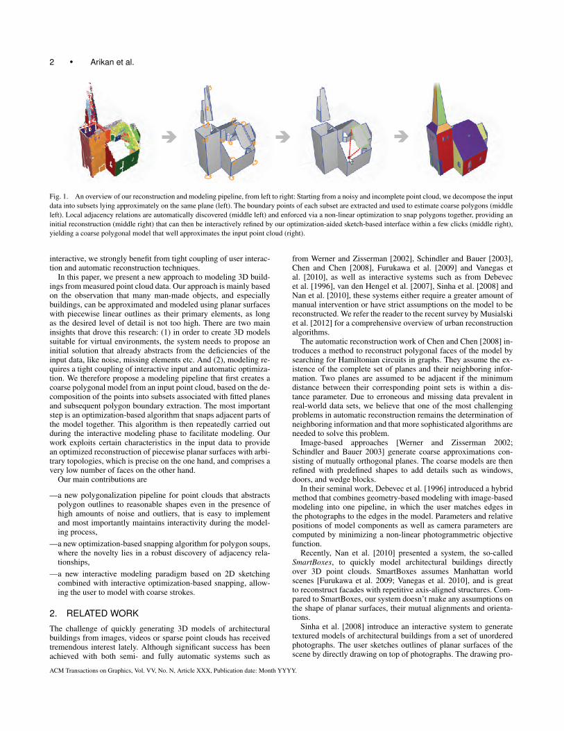
Fig. 1. An overview of our reconstruction and modeling pipeline, from left to right: Starting from a noisy and incomplete point cloud, we decompose the inputdata into subsets lying approximately on the same plane (left). The boundary points of each subset are extracted and used to estimate coarse polygons (middleleft). Local adjacency relations are automatically discovered (middle left) and enforced via a non-linear optimization to snap polygons together, providing aninitial reconstruction (middle right) that can then be interactively refined by our optimization-aided sketch-based interface within a few clicks (middle right),yielding a coarse polygonal model that well approximates the input point cloud (right).

interactive, we strongly benefit from tight coupling of user interac-tion and automatic reconstruction techniques.

In this paper, we present a new approach to modeling 3D build-ings from measured point cloud data. Our approach is mainly basedon the observation that many man-made objects, and especiallybuildings, can be approximated and modeled using planar surfaceswith piecewise linear outlines as their primary elements, as longas the desired level of detail is not too high. There are two maininsights that drove this research: (1) in order to create 3D modelssuitable for virtual environments, the system needs to propose aninitial solution that already abstracts from the deficiencies of theinput data, like noise, missing elements etc. And (2), modeling re-quires a tight coupling of interactive input and automatic optimiza-tion. We therefore propose a modeling pipeline that first creates acoarse polygonal model from an input point cloud, based on the de-composition of the points into subsets associated with fitted planesand subsequent polygon boundary extraction. The most importantstep is an optimization-based algorithm that snaps adjacent parts ofthe model together. This algorithm is then repeatedly carried outduring the interactive modeling phase to facilitate modeling. Ourwork exploits certain characteristics in the input data to providean optimized reconstruction of piecewise planar surfaces with arbi-trary topologies, which is precise on the one hand, and comprises avery low number of faces on the other hand.

Our main contributions are

—a new polygonalization pipeline for point clouds that abstractspolygon outlines to reasonable shapes even in the presence ofhigh amounts of noise and outliers, that is easy to implementand most importantly maintains interactivity during the model-ing process,

—a new optimization-based snapping algorithm for polygon soups,where the novelty lies in a robust discovery of adjacency rela-tionships,

—a new interactive modeling paradigm based on 2D sketchingcombined with interactive optimization-based snapping, allow-ing the user to model with coarse strokes.

2. RELATED WORK

The challenge of quickly generating 3D models of architecturalbuildings from images, videos or sparse point clouds has receivedtremendous interest lately. Although significant success has beenachieved with both semi- and fully automatic systems such as

from Werner and Zisserman [2002], Schindler and Bauer [2003],Chen and Chen [2008], Furukawa et al. [2009] and Vanegas etal. [2010], as well as interactive systems such as from Debevecet al. [1996], van den Hengel et al. [2007], Sinha et al. [2008] andNan et al. [2010], these systems either require a greater amount ofmanual intervention or have strict assumptions on the model to bereconstructed. We refer the reader to the recent survey by Musialskiet al. [2012] for a comprehensive overview of urban reconstructionalgorithms.

The automatic reconstruction work of Chen and Chen [2008] in-troduces a method to reconstruct polygonal faces of the model bysearching for Hamiltonian circuits in graphs. They assume the ex-istence of the complete set of planes and their neighboring infor-mation. Two planes are assumed to be adjacent if the minimumdistance between their corresponding point sets is within a dis-tance parameter. Due to erroneous and missing data prevalent inreal-world data sets, we believe that one of the most challengingproblems in automatic reconstruction remains the determination ofneighboring information and that more sophisticated algorithms areneeded to solve this problem.

Image-based approaches [Werner and Zisserman 2002;Schindler and Bauer 2003] generate coarse approximations con-sisting of mutually orthogonal planes. The coarse models are thenrefined with predefined shapes to add details such as windows,doors, and wedge blocks.

In their seminal work, Debevec et al. [1996] introduced a hybridmethod that combines geometry-based modeling with image-basedmodeling into one pipeline, in which the user matches edges inthe photographs to the edges in the model. Parameters and relativepositions of model components as well as camera parameters arecomputed by minimizing a non-linear photogrammetric objectivefunction.

Recently, Nan et al. [2010] presented a system, the so-calledSmartBoxes, to quickly model architectural buildings directlyover 3D point clouds. SmartBoxes assumes Manhattan worldscenes [Furukawa et al. 2009; Vanegas et al. 2010], and is greatto reconstruct facades with repetitive axis-aligned structures. Com-pared to SmartBoxes, our system doesn’t make any assumptions onthe shape of planar surfaces, their mutual alignments and orienta-tions.

Sinha et al. [2008] introduce an interactive system to generatetextured models of architectural buildings from a set of unorderedphotographs. The user sketches outlines of planar surfaces of thescene by directly drawing on top of photographs. The drawing pro-


O-Snap: Optimization-Based Snapping for Modeling Architecture • 3

cess is made easier by snapping edges automatically to vanishingpoint directions and to previously sketched edges. Compared to ourapproach, their system still needs a precise drawing of polygons,since they do not automatically estimate polygon boundaries, andsnapping is induced by a simple proximity criteria, while our sys-tem reliably extracts adjacency relations between elements of thepolygons.

The VideoTrace system proposed by van den Hengel et al. [2007]interactively generates 3D models of objects from video. The usertraces polygon boundaries over video frames. While in the work ofSinha a single image is sufficient to accurately reconstruct polyg-onal faces, VideoTrace repeatedly re-estimates the 3D model byusing other frames.

A large number of mesh reconstruction methods have beenproposed over the years: popular approaches include Extendedmarching cubes by Kobbelt et al. [2001], the Delaunay refine-ment paradigm [Boissonnat and Oudot 2005] and implicit ap-proaches [Kazhdan et al. 2006; Alliez et al. 2007; Schnabel et al.2009]. Typically, all these methods need to generate high resolu-tion meshes in order to recover sharp edges. More recently, Salmanet al. [2010] have improved the accuracy of reconstructions for aprescribed mesh size while ensuring a faithful representation ofsharp edges. Still, their method does not yield models of low facecount and visual quality as required in this work (cf. Figure 15).Instead of applying an extensive post-processing pipeline (e.g. cen-tered around Cohen-Steiner et al.’s shape approximation [2004]),we propose to integrate all requirements into a single optimized al-gorithm: our method fits median planes to the input data, accuratelyreconstructs sharp edges from the intersection of these planes andgenerates coarse polygonal models (with the complexity definedby the number of planes). Most importantly, our method is good athandling surfaces with boundaries: all our input data is incomplete,with missing parts and holes due to the acquisition process.

Recent commercial systems such as SketchUp have been de-signed to quickly create 3D models from users’ sketches. ThePointools plugin for SketchUp [2011] allows users to model di-rectly over 3D point clouds, but the accuracy of the reconstructiondepends on the skills and patience of the user, since the sketchedgeometry has to be manually aligned to the point cloud by visualinspection. In addition, the plugin offers a simple snapping tool thatallows snapping the endpoint of a sketched line to a nearby pointin the point cloud. In practice, this feature can be used to coarselysketch the floorplan of a building, but is impractical for more de-tailed modeling tasks due to the noise inherent in point clouds, asthere is no way to align a primitive to a set of points. Furthermore,gaps that appear in the modeling process have to be closed man-ually by moving edges. In contrast, we optimally reconstruct pla-nar primitives by least-median fitting to the point data. Moreover,we automatically discover adjacency relations, which allows us torun a planarity-preserving optimization-based snapping algorithmto close the model.

GlobFit, recently introduced by Li et al. [2011], iteratively learnsmutual relations among primitives obtained by the RANSAC algo-rithm [Schnabel et al. 2007]. Their system seems to be complemen-tary to ours: While they focus on discovering global relations (likeorthogonality, coplanarity, etc.) among parts of the model to correctthe primitives, our strength lies in the automatic discovery of localadjacency relations between polygon elements. To produce a finalmodel (which is not their primary goal), Li et al. only extrapolateand compute pairwise primitive intersections. While it is relativelyeasy to locally extend individual polygons, intersections of multi-ple primitives can be highly complex and reconstruction becomesnon-trivial.

3. OVERVIEW

Our system takes as input a set of 3D points, for example froma laser scanner, photogrammetric reconstruction or similar source.The goal is to create a polygonal model suitable for interactive ap-plications and not influenced by the noise and holes inherent in theinput data. The reconstructed polygonal model will be watertightwherever feasible – in this paper we shall denote such a model aclosed model. It is important to emphasize that we do not assumeour target surfaces to be closed in a topological sense.

Modeling consists of two phases: an automatic phase that cre-ates an initial model, and an interactive phase that is aided byoptimization-based snapping.

3.1 Automatic Phase

In the automatic phase, the input data is decomposed into subsetslying approximately on the same plane (Figure 1, left). Through-out the paper, we refer to these subsets as segments. For each suchsegment, boundary polygons are estimated in the polygonalizationstep (Section 4, Figures 1 middle left and 3). The resulting modelstill has holes and is not well aligned.

We therefore introduce an intelligent snapping algorithm (Sec-tion 5) that constrains and optimizes the locally fitted planes andtheir corresponding polygons. The local fit of the planes is de-termined by how well the planes approximate the observed pointcloud data, while the mutual spatial relations, i.e., adjacency rela-tions between polygon elements, are iteratively computed and en-forced through a non-linear optimization. This “intelligent snap-ping” is a crucial part of our approach: Instead of simply snappingto existing geometry or features within a given distance [Sinha et al.2008; van den Hengel et al. 2007], we define a feature-sensitivematching and pruning algorithm to discover a robust set of adja-cency relations among parts of the polygons (Figure 1, middle left).The polygons are then aligned by enforcing the extracted relations,while best fitting to the input data and maintaining the planarity ofthe polygons (Figure 1, middle right).

Note that while a completely automatic reconstruction of a wholebuilding can hardly be achieved due to erroneous and missing data,our automatic phase produces results that are comparable to previ-ous automatic systems, for example Chen and Chen [2008], whoassume the existence of a complete set of planes.

3.2 Interactive Phase

Since the initial geometry proposal from the automatic phase cannot guarantee a perfect solution in all cases, the interactive phaseprovides a simple and intuitive sketch-based user interface (Sec-tion 6) that directly interoperates with the optimization routines.Even though such manual interventions can not be completelyomitted, the novel system differs significantly from other 3D mod-eling techniques by exploiting the previous analysis: Due to theknown supporting planes, the modeling complexity is reduced froma 3D to a 2D problem. This allows the user to model the neces-sary changes with a few simple and loose strokes on a flat layer, asthe exact alignment is performed interactively by the optimization-based snapping algorithm (Figure 1 middle right).

4. POLYGONALIZATION

We use a local RANSAC-based method [Schnabel et al. 2007] todecompose the input point cloud into subsets (referred to as seg-ments), each lying approximately on a plane, and a set of unclaimedpoints. Even though the decomposition requires normal informa-


4 • Arikan et al.

Fig. 2. The first step of the automatic reconstruction pipeline, a localRANSAC-based method, may capture nearby parallel structures (e.g. win-dows and facade) as a single segment (left). The least-median of squaresmethod is used to fit a plane to the points of the dominant structure (mid-dle left). By applying k-means clustering (k = 2) (and subsequent auto-matic polygonalization and optimization) in the interactive modeling phase,a more detailed hierarchical reconstruction (middle right, right) is achieved.

tion, the correctness of normals close to sharp edges is not criticalfor the subsequent estimation of plane primitives (Section 4.1.1)and the rest of our pipeline. Hence, our implementation approxi-mates 3D normal vectors from point positions by applying a localPCA [Jolliffe 2002] with fixed size neighborhoods.

A segment may consist of multiple connected components (e.g.,front faces of all individual balconies on a facade), which are laterseparated by the boundary extraction algorithm (Section 4.1.2).

The goal of the polygonalization step is to divide the segmentsfrom the RANSAC stage into connected components, and approx-imate their outlines by coarse polygons. In the first step, we divideeach segment into one or several connected components, and ex-tract their ordered boundary points (Figure 3 top left), which act asinitial polygons. Since the extracted boundaries are generally noisy,we cannot assume that we have high-quality vertex normal orienta-tions. In the second step, we compute a smooth region around eachpoint (Figure 3 top right), to which we then apply a local PCA toestimate initial 2D vertex normals (Figure 3 middle left). Finally,we reconstruct 2D vertex normals based on their initial values anda neighborhood relationship derived from the smooth regions (Fig-ure 3 middle right), and use the reconstructed normal vectors tocompute consistent vertex positions (Figure 3 bottom left). Thisprocess straightens the initial boundaries and thus provides a polyg-onal approximation of the 2D components on a coarse scale (Fig-ure 3 bottom right).

4.1 Initialization

4.1.1 Plane fitting. The polygonalization is computed in 2Dspace defined by the segment plane. The first step is therefore fit-ting a plane to all the points contained in a segment obtained byRANSAC. As depicted in Figure 2 (left), nearby parallel structures(e.g., main facade and windows) may have been detected as a singlesegment. We therefore apply a Least Median of Squares (LMS) es-timator [Rousseeuw and Leroy 1987], which consistently finds themain structure (see Figure 2 middle left), as it is capable of fittinga model to data that contains up to 50% outliers.

4.1.2 Boundary extraction. In order to divide each segmentinto connected components and extract their ordered boundarypoints, we employ 2D α-shapes [Edelsbrunner and Mucke 1994](with α controlling the number of connected components and thelevel of detail of their boundaries) on the segment points projectedto the median plane. The family of 2D α-shapes of the set of pro-

p

Qp

Fig. 3. Overview of our polygonalization pipeline. Ordered boundarypoints (initial polygon) of a connected component are extracted (top left).By applying PCA to smooth regions Q (top right), vertex normals are ini-tialized (middle left). Initial vertex normals are smoothed over neighboringvertices (with p and q neighboring if they are mutually contained in theirrespective smooth regions) (middle right) and used to compute consistentvertex positions (bottom left). Finally, a corner detection algorithm extractsthe approximating polygon.

jected segment points S is implicitly represented by the Delaunaytriangulation of S. Each element (vertices, edges and faces) of theDelaunay triangulation is associated with an interval that specifiesfor which values of α the element belongs to the α-shape. The con-nectivity of the Delaunay triangulation and the classification of itselements with respect to the α-shape is then used to extract the con-nected components and their ordered boundary points. We estimateα using the average distance between neighboring points.

4.2 Polygon Straightening

The goal of this step is to robustly estimate for each boundary acoarse polygon that approximates the original shape’s outline. Mostsurfaces used in architecture, especially at the level of detail rel-evant for polygonal modeling, are bounded by straight lines thatmeet in sharp corners. We also require from our method that it isfast, since we need interactivity during the modeling process (seeSection 6.6).

Our method is inspired by the `1-sparse method [Avron et al.2010] for the reconstruction of piecewise smooth surfaces. How-ever, we found the `1 formulation computationally too expensive,compared to our `2 approach counting only a few or even no re-weighted iterations (the `1 formulation’s second-order cone pro-gramming solver needs to solve a series of linear systems of com-parable dimension to our setting). We tackle stability issues inher-ent to least-squares approaches (such as sensitivity to outliers) withstatistical methods. In particular, we rely on the forward searchmethod [Atkinson and Riani 2000] and present a novel methodcombining the simplicity of least-squares minimization with thestrength of robust statistics.



4.2.1 Neighborhood estimation. Similar to Fleishman et al.’sapproach [2005], we classify a locally smooth region around eachvertex by applying the forward search method, which preservessharp features and is robust to noise and outliers. The main ideain forward search is to start from a small outlier-free neighborhoodQ and to iteratively extend the set Q until a termination criterionis met. Starting from Q and the model (in our case, a line) that isfitted to the points in Q, one iteratively adds one point to the setQ (the point with lowest residual) and updates the model at eachiteration, until the diameter of Q exceeds a threshold dmax. Fig-ure 3, top right, shows an example of a smooth region around apoint p computed with forward search. Two polygon vertices pand q are said to be neighboring, if q ∈ Qp and vice versa. The di-ameter threshold dmax is the only parameter that affects the outputof our polygonalization method. Since dmax controls the local re-gion sizes, we avoid high values of dmax (usually set to minimumexpected feature size) to prevent oversmoothing of sharp features.

4.2.2 2D Normal estimation. We then estimate consistentlyoriented vertex normal vectors (Figure 3, middle right) based onthe neighborhood relationship computed by the prior step. As inAvron et al. [2010], our least-squares minimization to reconstructvertex normals consists of two terms and is formulated as:

E1 =∑

(p,q)∈N

wp,q‖np − nq‖2 + λ∑p

‖np − n0p‖2. (1)

The first term minimizes the normal differences and extends overthe set N of all neighboring vertices. The second term prevents thevertex normals n from deviating too much from their initial orien-tations n0. The weighting function wp,q in Equation 1 penalizesvariations in normal directions, and is given by the Gaussian filter:

wp,q = e−(θp,q/σ)2, (2)

where θp,q is the angle between the normal vectors np and nq andσ is a parameter set to 20 degrees in all our examples.

The normal vectors are initialized (cf. Figure 3 middle left) byapplying PCA to the local smooth regions computed by the priorstep. The consistency of the initial normal orientations is providedby the order of the boundary points.

4.2.3 2D Polygon smoothing. We then compute consistent ver-tex positions (Figure 3, bottom left) by displacing polygon verticesin normal direction, i.e.,

p′ = p + tpnp.

Similar to Avron et al. [2010], the new vertex positions p′ are com-puted as the minimizer of the energy function

E2 = E2,s +E2,init (3)

with

E2,s =∑

(p,q)∈N

wp,q

(∣∣(p′ − q′) · nq∣∣2 +

∣∣(q′ − p′) · np∣∣2)

and

E2,init = µ∑p

t2p.

The first term smoothes (straightens) the polygon boundary by min-imizing the deviation of q from the tangent through p weightedaccording to the confidence measure wp,q (Equation 2) and viceversa. The second term prevents the polygon vertices from devi-ating too much from their initial positions and as a consequenceavoids shrinking of the polygon.

Both functionals E1 and E2 (Equations 1 and 3) are minimizedusing a Gauss-Newton method. Since we use forward search to re-construct outlier-free regions, we require only three re-weighted it-erations to minimize E1 and a single iteration to minimize E2. Theweight parameters λ and µ are set to 0.1 in our data sets.

4.3 Polygon Extraction

The process described above provides us with a set of straightenedboundary points with high-quality vertex normals, which are thenused by a simple corner detection algorithm to extract approximat-ing coarse polygons (Figure 3, bottom right).

We classify a vertex as an edge vertex if its normal vector isalmost parallel to the normal vector of the succeeding and preced-ing vertex, respectively. Then we approximate sequences of edgevertices in a least-squares sense and obtain edge lines. A corner isdetected at the intersection point of two successive lines. Note thatvertices that are isolated in our neighborhood relationship graphare potential outliers or influenced by noise inherent in the initialboundaries, and thus not used by the corner detection algorithm.

5. POLYGON SOUP SNAPPING

The result of the polygonalization step is a soup of unconnectedpolygons P = {P1, . . . , Pn}. The snapping process aims at clos-ing the holes between the polygons of the polygon soup, and isused both in the initial automatic reconstruction and during interac-tive modeling. Snapping iteratively pulls polygon vertices towardsother polygons, while simultaneously re-fitting P to the underlyingpoint cloud and preserving the planarity of polygons. Each iterationconsists of the following two steps:

—Robust search for adjacencies, which for each vertex identifiesthe possible matches to other vertices, edges or faces and dis-cards false ones.

—Optimization, which enforces the set of discovered adjacency re-lations to snap the polygon soup together.

The process terminates when the polygon soup stabilizes, i.e., it be-comes a closed model and satisfies the requirements given by theconstraints. Our snapping process is related to Botsch et al. [2006]and Kilian et al. [2008], however our system requires the optimiza-tion for various other constraints and in particular, the relations be-tween the polygons are not known a priori. We now describe thesteps in detail.

5.1 Robust Search for Adjacencies

The problem of matching the elements of the polygon soup to aclosed model in a feature-aware manner is inherently ill-defined.The expected bad quality of the real-world data sets and the lackof any high-level input to the reconstruction pipeline (such asshape templates or semantic information) prevent a rigorous math-ematical definition. Instead, we propose an automatic and robustalgorithm based on stable vertex-vertex/edge/face and edge-edgematches.

Adjacencies in the model are discovered by searching formatches between polygon elements. There are five mechanismsthat constrain the allowed matches: (1) An auxiliary global parame-ter rmax defines the maximal gap size to be closed in the model. (2)Intrinsic stability locally avoids self-intersections, flip-overs, edgeand diagonal collapses. (3) An extended set of matching candidatesallows more degrees of freedom (thus a more connected model)where (2) is too restrictive. (4) Local pruning fixes problems mostlyintroduced by (3), and (5) global pruning prevents degeneration of


6 • Arikan et al.

polygons (especially of thin features) by considering global issuesof matches affecting more than two polygons. We first describe thedifferent match types, constrained by (1-3), and then show localand global pruning. Please note that the choice of rmax doesn’t in-fluence the stability of the pruning algorithms, but only defines themaximal gap size.

5.1.1 Vertex-vertex matching. We define an adaptive searchradius for each vertex of the model. The requirement of intrin-sic stability bounds the search radius to half the minimal distancefrom p to the polygon’s boundary, d∂(p) := mine∈∂P \p d(p, e),where ∂P \ p denotes the polygon boundary after removal of pand its incident edges. Half the distance d∂ prevents vertices be-ing matched across polygon edges (self-intersections, flip-overs) orvertices (edge or diagonal collapses). To respect the given upperbound, we define r(p) := min(rmax, d∂(p)/2) as the adaptivesearch radius of p.

The candidate set of matches for a vertex p comprises all verticesof P \P within search distance r(p). If this candidate set is empty,the closest vertex in P\P (if not further than rmax) is included. Bydoing so, we may violate intrinsic stability intentionally to maintainsufficient degrees of freedom. A subsequent pruning step, describedbelow, will restore validity at a later stage, if necessary. We definerc(p) := max(r(p),min(dc, rmax)) (with dc being the distanceof p to its closest vertex in P \P ) as the extended search radius ofp.

A priori, two vertices p and q are considered matching, if theyare mutually included in their respective extended search radii,

‖p− q‖ ≤ min(rc(p), rc(q)).

Finally, two matching vertices are supposed to collapse into a cor-ner point at the later optimization stage. Such a corner point is inci-dent to the intersection line l of the two corresponding supportingplanes. Consequently, we further require a pair of matching verticesto be in feasible distance to l,

d(l,p) ≤ rc(p) and d(l,q) ≤ rc(q).

Please note that the computation of l is numerically stable, as theRANSAC stage gives a priori knowledge about polygons in thesame supporting plane.

5.1.2 Vertex-edge matching. In a similar fashion to vertex-vertex matches, we establish correspondences between ver-tices and edges. We assign a search radius to each edgee = (p0,p1) as the minimal search radius of its end points,r(e) = min(r(p0), r(p1)). A vertex p is matched to an edgee if its orthogonal projection onto the line spanned by e is in theedge’s interior, and – analogous to a vertex-vertex match – the twofollowing expressions hold true:

d(p, e) ≤ min(r(p), r(e)),

and

d(l,p) ≤ r(p) and d(l, e) ≤ r(e),

where l is the common intersection line of the corresponding sup-porting planes.

5.1.3 Other matches. To complete the survey of matches, avertex p is paired with a face f if its orthogonal projection ontothe plane spanned by f is in the face’s interior and no further thansearch radius r(p).

Based on the vertex-vertex and vertex-edge matches, we mayfurther derive edge-edge matches: Two edges are said to match if

p q

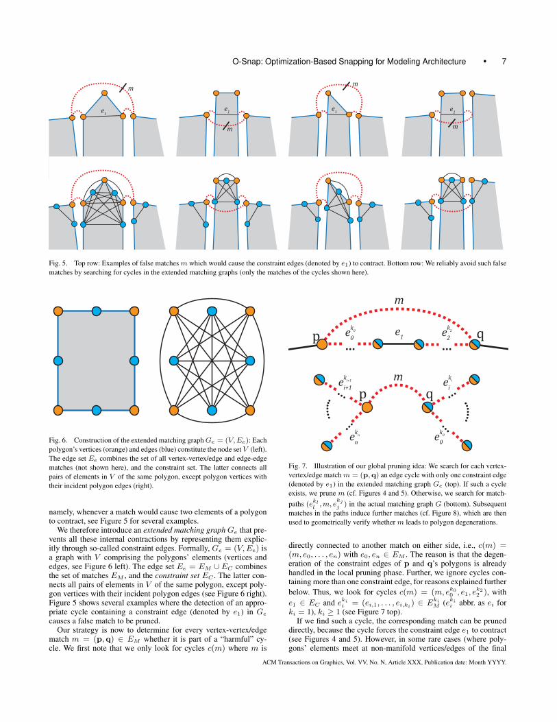
m

e0 e2e1

Fig. 4. The false match m = (p,q), which forces the center polygon’sedge e1 to collapse and thus violates the intrinsic stability, is reliably de-tected by our global pruning strategy.

their endpoints either induce two vertex-vertex matches, a vertex-vertex and a vertex-edge match or two vertex-edge matches. Edge-edge matches are used only in the matching and global pruningstage and not for optimization, as their contribution to reconstruc-tion is implicitly included through vertex-vertex/edge matches.The same holds in an even stricter sense for edge-face and face-face matches, which are either implied by vertex-vertex/edge/facematches or are not present in the data due to occlusion in the acqui-sition process.

5.1.4 Local pruning. The vertex-vertex matching yields gen-erally stable results. A few false matches, which result from theinclusion of closest vertices in candidate sets, are corrected in thefollowing pruning step: Consider two or more vertices qi of poly-gon Q being matched to a vertex p ∈ P . This clearly violatesthe intrinsic stability requirement for Q and we remove all but theclosest matching pair. This and all subsequent pruning steps are im-plemented on a graph representationG = (V,EM ) of the matches,with all vertices and edges of P comprising V and the edge setEMbeing given by the set of all matches obtained from above (exceptvertex-face matches). Pruning at this point boils down to investi-gating all one-ring neighborhoods of G.

Similar to vertex-vertex matching, intrinsic stability demands thepruning of those vertex-edge matches where a vertex correspondsto multiple non-adjacent edges of a polygon. This can naturallyhappen due to overlapping search cylinders (with radii r(e)) aroundedges. Using the graph G, we compress this subset of matches tothe closest vertex-edge match.

5.1.5 Global pruning. Up to now, the matches have been ob-tained on a local level only. They disregard any global issues af-fecting more than two polygons. Consider the situation in Fig-ure 4, with three polygons stringing together and several of thecorner points being matched. The vertex-vertex match between pand q, jumping the center polygon, is not feasible, as it impliesa degeneration of the center polygon’s edge. Such a degenerationhappens when certain polygon elements (vertices/edges) are con-nected through matches so that they form a cycle. The reason isthat we have to assume that all polygon elements connected throughmatches might be joined to the same location during the optimiza-tion phase. In this section we therefore present our approach to de-fine and find such cycles. We also show a second approach basedon geometric tests for cases where the detection of cycles doesn’tnecessarily imply a degeneration.

For the example in Figure 4, to detect the contraction of theedge e1, it would be sufficient to extend the edge set EM in thematching graph G defined earlier by the actual polygon edges, andfind the cycle (m, e0, e1, e2) in the resulting graph. However, thereare many other cases that would lead to a polygon degeneration,



e1e1e1e1

m

m

m

m

Fig. 5. Top row: Examples of false matches m which would cause the constraint edges (denoted by e1) to contract. Bottom row: We reliably avoid such falsematches by searching for cycles in the extended matching graphs (only the matches of the cycles shown here).

Fig. 6. Construction of the extended matching graph Ge = (V,Ee): Eachpolygon’s vertices (orange) and edges (blue) constitute the node set V (left).The edge set Ee combines the set of all vertex-vertex/edge and edge-edgematches (not shown here), and the constraint set. The latter connects allpairs of elements in V of the same polygon, except polygon vertices withtheir incident polygon edges (right).

namely, whenever a match would cause two elements of a polygonto contract, see Figure 5 for several examples.

We therefore introduce an extended matching graphGe that pre-vents all these internal contractions by representing them explic-itly through so-called constraint edges. Formally, Ge = (V,Ee) isa graph with V comprising the polygons’ elements (vertices andedges, see Figure 6 left). The edge set Ee = EM ∪ EC combinesthe set of matches EM , and the constraint set EC . The latter con-nects all pairs of elements in V of the same polygon, except poly-gon vertices with their incident polygon edges (see Figure 6 right).Figure 5 shows several examples where the detection of an appro-priate cycle containing a constraint edge (denoted by e1) in Gecauses a false match to be pruned.

Our strategy is now to determine for every vertex-vertex/edgematch m = (p,q) ∈ EM whether it is part of a “harmful” cy-cle. We first note that we only look for cycles c(m) where m is

m

ek0

0ek2

2

... ...e

1p q

m

ek0

0

...p q

...

eki

i

ekn

n

eki+1

i+1

.......

...

...

.......

Fig. 7. Illustration of our global pruning idea: We search for each vertex-vertex/edge match m = (p,q) an edge cycle with only one constraint edge(denoted by e1) in the extended matching graph Ge (top). If such a cycleexists, we prune m (cf. Figures 4 and 5). Otherwise, we search for match-paths (e

kll ,m, e

kjj ) in the actual matching graph G (bottom). Subsequent

matches in the paths induce further matches (cf. Figure 8), which are thenused to geometrically verify whether m leads to polygon degenerations.

directly connected to another match on either side, i.e., c(m) =(m, e0, . . . , en) with e0, en ∈ EM . The reason is that the degen-eration of the constraint edges of p and q’s polygons is alreadyhandled in the local pruning phase. Further, we ignore cycles con-taining more than one constraint edge, for reasons explained furtherbelow. Thus, we look for cycles c(m) = (m, ek00 , e1, e

k22 ), with

e1 ∈ EC and ekii = (ei,1, . . . , ei,ki) ∈ EkiM (ekii abbr. as ei forki = 1), ki ≥ 1 (see Figure 7 top).

If we find such a cycle, the corresponding match can be pruneddirectly, because the cycle forces the constraint edge e1 to contract(see Figures 4 and 5). However, in some rare cases (where poly-gons’ elements meet at non-manifold vertices/edges of the final


8 • Arikan et al.

m

mi

e0

e1

e2

e3

e4

m

mi

e0

e1 e2

e3 e4

Fig. 8. Cycles (here (m, e0, e1, e2, e3, e4)) in the extended matchinggraphs Ge containing more than one constraint edge can be “harmful”(right) or not (left), and thus are not a good indicator for pruning. Insteadwe geometrically verify whether the induced matches (denoted in green bymi) resulting from subsequent matches (e0,m, e4) in the matching graphsG cause polygon degenerations. Please note that in the right image, m is se-lected in the matching phase due to large search radii of the correspondingvertices (we show only a part of the polygons here).

model) we also observed the pruning of a few “correct” matches.For the convergence of n polygon elements to the same location,(n2

)connections (matches) are possible, but only n − 1 involving

all those n elements are sufficient. Thus in practice, the pruning ofa few “correct” matches doesn’t indicate a problem.

Most of the degenerations in the model can already be avoidedby pruning cycles with one constraint edge. However, there are alsosome cases involving several constraint edges, see Figure 8 right.Unfortunately, this situation cannot be detected unambiguously bysearching for cycles, as can be seen in Figure 8 left. To solve thisproblem, we present a more general approach that is based on in-vestigating sequences of matches. Such sequences induce furthermatches between the elements they connect, in the sense that inthe optimization phase, these elements will also be joined. We thusneed to verify whether the induced matches do not cause polygondegenerations.

Formally, for a matchm, we search for paths (ekll ,m, e

kjj ) (with

kl, kj ≥ 0) in the actual matching graph G (see Figure 7 bottom).We then check whether all of the induced matches mi are in EMas well. For every match that is not in EM , we need to verify ge-ometrically whether it would lead to a polygon degeneration. Herewe note that an induced match does not necessarily join the at-tached elements directly (e.g., two subsequent vertex-edge matchesm1 = (p, e) and m2 = (e,q) do not induce the vertex-vertexmatch m3 = (p,q), but both vertices project to the same edge).To geometrically verify whether an induced match leads to any de-generation, we project the vertices and/or edge endpoints of thematch onto the common intersection line l of the polygons’ sup-porting planes. We prune m if one of the thus-modified polygons(with projected vertices/edges) has a flipped normal vector orien-tation (flip-over) or has self-intersections. Note that the number ofpaths to investigate is typically low because paths containing onlymatches stay localized.

5.2 Optimization

Based on the discovered adjacencies, we transform the polygonsto optimally align with each other, while preserving their planarityand fitting to the input point cloud.

As in Kilian et al. [2008], we introduce a Cartesian coordinatesystem in the plane of each P ∈ P , with origin o and basis vec-tors f1 and f2, and represent a point p ∈ P by the coordinates(px, py), so that p = o + pxf1 + pyf2. During the optimization,

in order to reduce the spatial gaps between adjacent polygons, thecoordinates (px, py) are displaced, while the Cartesian coordinatesystems undergo a spatial motion. We linearize the spatial motionof each coordinate system by representing the displacement of eachpoint through the velocity vector field of an instantaneous motion,given by v(x) = c + c × x. Thus the position of a vertex p ∈ Piduring the optimization can be written as

p = oi+ ci+ci×oi+px(fi1 +ci×fi1)+py(fi2 +ci×fi2) (4)

in the unknown parameters ci, ci ∈ R3 of the velocity vector fieldattached to Pi and in the unknown coordinates (px, py) (this canbe derived by applying the displacement x′ = x + v(x) for x ∈{oi,oi + fi1 ,oi + fi2}).

5.2.1 Snapping. With the adjacency relations discovered bythe prior step, we measure the snapping error as

Esnap =∑i,j,k,l

d2(pi,pj) + d2(pi, ek) + d2(pi, Pl),

where d2(pi, ·) denotes the distance of vertex pi to the vertex pj ,edge ek and face Pl, respectively.

5.2.2 Point cloud deviation. For the polygon soup P not to de-viate too much from the input point cloud, we use the referenceterm

Eref =

|P|∑l=1

|Pl |∑i=1

d2(pi(l), Pinitl ). (5)

The above equation minimizes the sum of squared distances of ver-tices pi(l) ∈ Pl to the initial planes P initl (see Section 4.1.1). Man-ually sketched polygons without underlying segments (Section 6.3)are excluded from Equation 5.

5.2.3 Orthogonality. In order to meet orthogonality con-straints that naturally exist in urban environments, we include thefollowing two terms

E⊥1=∑i,j

wij(ni · nj)2 (6)

and

E⊥2=

|P|∑l=1

|Pl |∑i=1

wi(l)(ei(l) · e(i+1)(l) mod |Pl |)2, (7)

which measure the orthogonality of adjacent polygons and succes-sive polygon edges, respectively. With the unit normal vector of Pgiven by n = f1 × f2, Equation 6 extends over all pairs of poly-gons, with wij = 1 for adjacent polygons with normals deviatingfrom orthogonality by less than π

9, and zero otherwise. Optimizing

for orthogonality of polygon boundary edges ei(l) in Equation 7(with wi(l) defined similar to wij for polygons) might result in de-generating edges of vanishing length. This problem is in particularevident in case of missing geometry and is overcome by minimiz-ing the sum of squared distances to current vertex positions p′i asfollows:

Ecur =∑i

d2(pi,p′i).

5.2.4 Global energy and weights. The above energy terms arecombined into the objective function

E = λsnapEsnap + λrefEref + λ⊥(E⊥1+E⊥2

) + λcurEcur,



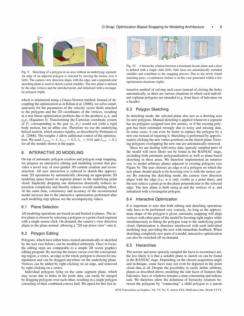
eye

Fig. 9. Sketching of a polygon in an area without an underlying segment:An edge of an adjacent polygon is selected by moving the mouse over it(left). The camera view direction aligns with the edge, and a perpendicularsketching plane is used to sketch a point (middle). The new plane is definedby the edge vertices and the sketched point, and initialized with a rectangu-lar polygon (right).

which is minimized using a Gauss-Newton method. Instead of de-coupling the optimization as in Kilian et al. [2008], we solve simul-taneously for the parameters of the velocity vector fields attachedto the polygons and the 2D coordinates of the vertices, resultingin a non-linear optimization problem due to the products pxci andpyci (Equation 4). Transforming the Cartesian coordinate systemof Pi corresponding to the pair (ci, ci) would not yield a rigidbody motion, but an affine one. Therefore we use the underlyinghelical motion, which ensures rigidity, as described by Pottmann etal. [2006]. The weights λ allow additional control of the optimiza-tion. We used λsnap = 1, λref = 0.5, λ⊥ = 0.01 and λcur = 0.1for all the models shown in the paper.

6. INTERACTIVE 2D MODELING

On top of automatic polygon creation and polygon soup snapping,we propose an interactive editing and modeling system that pro-vides a novel way of user-guided 3D content creation and recon-struction. All user interaction is reduced to sketch-like approxi-mate 2D operations by automatically choosing an appropriate 2Dmodeling space based on segment planes in the underlying pointcloud. Implicitly dropping one dimension drastically reduces in-teraction complexity and thereby reduces overall modeling effort.At the same time, consistency and accuracy of the reconstructedmodel increase due to the interactive optimization performed aftereach modeling step (please see the accompanying video).

6.1 Plane Selection

All modeling operations are based on and limited to planes. The ac-tive plane is chosen by selecting a polygon or a point cloud segmentwith a single mouse click. On demand, the camera’s view directionaligns to the plane normal, allowing a “2D top-down view” onto it.

6.2 Polygon Editing

Polygons, which have either been created automatically or sketchedby the user (see below), can be modified arbitrarily. Once in focus,the editing steps are comparable to a simple 2D vector graphicsediting program: By moving the mouse cursor over the correspond-ing region, a vertex, an edge or the whole polygon is chosen for ma-nipulation and can be dragged anywhere on the underlying plane.Vertices can be added by right-clicking on an edge, and removedby right-clicking on a vertex.

Individual polygons lying on the same segment plane, whichmay occur due to holes in the point data, can easily be mergedby dragging polygons over each other, resulting in a single polygonconsisting of their combined convex hull. We opted for this fast in-

Fig. 10. A hierarchy relation between a dominant facade plane and a dooris defined with a single click (left). Side faces are automatically extruded(middle) and contribute to the snapping process: Due to the newly foundmatching pairs, a continuous surface is in this case generated within a fewoptimization iterations (right).

teractive method of solving such cases instead of closing the holesautomatically, as there are various situations in which such individ-ual coplanar polygons are intended (e.g. front faces of balconies ona facade).

6.3 Polygon Sketching

In sketching mode, the selected plane also acts as a drawing areafor new polygons. Manual sketching is applied whenever a segmenthas no polygons assigned (too few points), or if the existing poly-gon has been estimated wrongly due to noisy and missing data.In some cases, it can even be faster to replace the polygon by anew one instead of repairing it. Sketching is performed by approxi-mately clicking the new vertex positions on the sketch plane. Exist-ing polygons overlapping the new one are automatically removed.

Since we are dealing with noisy data, sparsely sampled parts ofthe model will most likely not be found in the RANSAC stage,excluding both automatic polygonalization as well as plane-basedsketching in these areas. We therefore implemented an intuitiveway to model arbitrary planes adjacent to existing polygons (seeFigure 9): The user chooses an edge e of a polygon on which thenew plane should attach to by hovering over it with the mouse cur-sor. By entering the sketching mode, the camera view directionaligns with the edge (i.e., e is only visible as a point then), andthe user selects a point p on the plane perpendicular to the selectededge. The new plane is built using p and the vertices of e, andinitialized with a rectangular polygon.

6.4 Interactive Optimization

It is important to note that both editing and sketching operationsonly have to be performed very coarsely. As long as the approxi-mate shape of the polygon is given, automatic snapping will alignvertices with other parts of the model by favoring right angles whilesimultaneously re-fitting the polygon soup to the underlying pointcloud. Optimization is therefore interleaved with each individualmodeling step, providing the user with immediate feedback. Whensketching completely new parts of a model, interactive optimizationcan also be switched off on-demand.

6.5 Hierarchies

The noisier and more sparsely sampled the faces to reconstruct are,the less likely it is that a suitable plane to sketch on can be foundin the RANSAC stage. Depending on the chosen acquisition angleand technique, some faces may not even be depicted in the pointcloud data at all. Despite the possibility to easily define arbitraryplanes as described above, modeling the side faces of features likebalconies, bays or windows remains a time-consuming and tedioustask. We therefore allow the definition of hierarchy relations be-tween the polygons by “connecting” a child polygon to a parent


10 • Arikan et al.

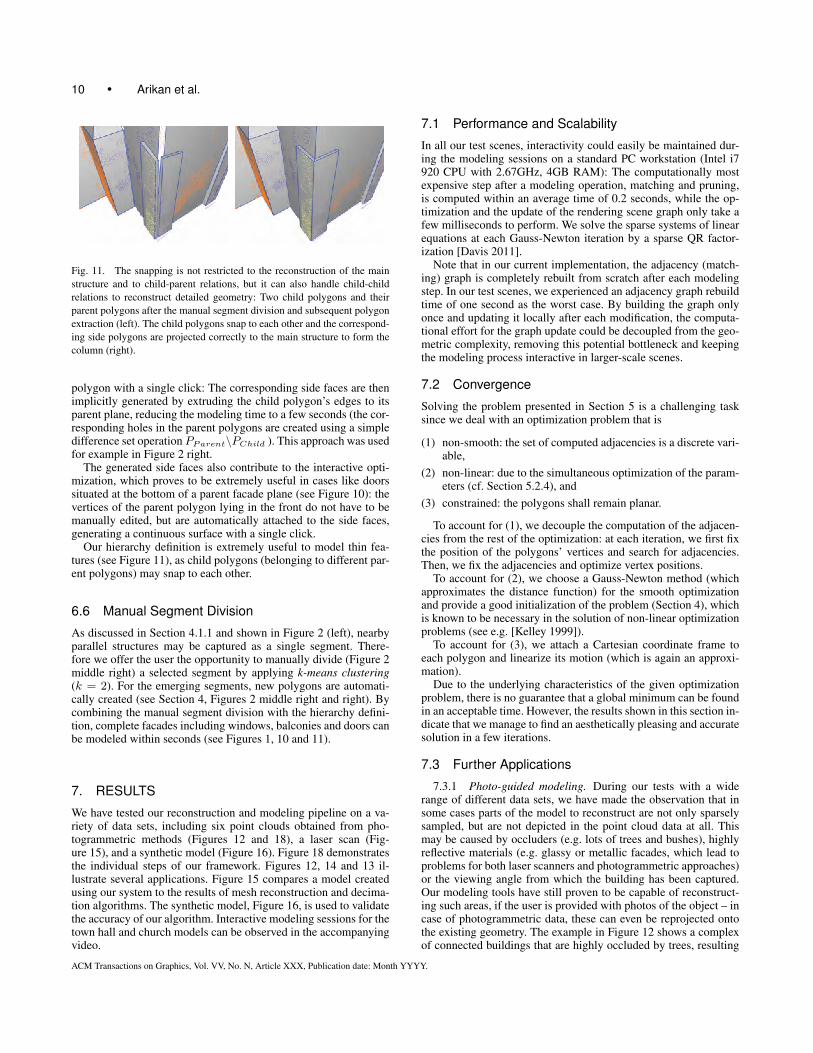
Fig. 11. The snapping is not restricted to the reconstruction of the mainstructure and to child-parent relations, but it can also handle child-childrelations to reconstruct detailed geometry: Two child polygons and theirparent polygons after the manual segment division and subsequent polygonextraction (left). The child polygons snap to each other and the correspond-ing side polygons are projected correctly to the main structure to form thecolumn (right).

polygon with a single click: The corresponding side faces are thenimplicitly generated by extruding the child polygon’s edges to itsparent plane, reducing the modeling time to a few seconds (the cor-responding holes in the parent polygons are created using a simpledifference set operation PParent\PChild ). This approach was usedfor example in Figure 2 right.

The generated side faces also contribute to the interactive opti-mization, which proves to be extremely useful in cases like doorssituated at the bottom of a parent facade plane (see Figure 10): thevertices of the parent polygon lying in the front do not have to bemanually edited, but are automatically attached to the side faces,generating a continuous surface with a single click.

Our hierarchy definition is extremely useful to model thin fea-tures (see Figure 11), as child polygons (belonging to different par-ent polygons) may snap to each other.

6.6 Manual Segment Division

As discussed in Section 4.1.1 and shown in Figure 2 (left), nearbyparallel structures may be captured as a single segment. There-fore we offer the user the opportunity to manually divide (Figure 2middle right) a selected segment by applying k-means clustering(k = 2). For the emerging segments, new polygons are automati-cally created (see Section 4, Figures 2 middle right and right). Bycombining the manual segment division with the hierarchy defini-tion, complete facades including windows, balconies and doors canbe modeled within seconds (see Figures 1, 10 and 11).

7. RESULTS

We have tested our reconstruction and modeling pipeline on a va-riety of data sets, including six point clouds obtained from pho-togrammetric methods (Figures 12 and 18), a laser scan (Fig-ure 15), and a synthetic model (Figure 16). Figure 18 demonstratesthe individual steps of our framework. Figures 12, 14 and 13 il-lustrate several applications. Figure 15 compares a model createdusing our system to the results of mesh reconstruction and decima-tion algorithms. The synthetic model, Figure 16, is used to validatethe accuracy of our algorithm. Interactive modeling sessions for thetown hall and church models can be observed in the accompanyingvideo.

7.1 Performance and Scalability

In all our test scenes, interactivity could easily be maintained dur-ing the modeling sessions on a standard PC workstation (Intel i7920 CPU with 2.67GHz, 4GB RAM): The computationally mostexpensive step after a modeling operation, matching and pruning,is computed within an average time of 0.2 seconds, while the op-timization and the update of the rendering scene graph only take afew milliseconds to perform. We solve the sparse systems of linearequations at each Gauss-Newton iteration by a sparse QR factor-ization [Davis 2011].

Note that in our current implementation, the adjacency (match-ing) graph is completely rebuilt from scratch after each modelingstep. In our test scenes, we experienced an adjacency graph rebuildtime of one second as the worst case. By building the graph onlyonce and updating it locally after each modification, the computa-tional effort for the graph update could be decoupled from the geo-metric complexity, removing this potential bottleneck and keepingthe modeling process interactive in larger-scale scenes.

7.2 Convergence

Solving the problem presented in Section 5 is a challenging tasksince we deal with an optimization problem that is

(1) non-smooth: the set of computed adjacencies is a discrete vari-able,

(2) non-linear: due to the simultaneous optimization of the param-eters (cf. Section 5.2.4), and

(3) constrained: the polygons shall remain planar.

To account for (1), we decouple the computation of the adjacen-cies from the rest of the optimization: at each iteration, we first fixthe position of the polygons’ vertices and search for adjacencies.Then, we fix the adjacencies and optimize vertex positions.

To account for (2), we choose a Gauss-Newton method (whichapproximates the distance function) for the smooth optimizationand provide a good initialization of the problem (Section 4), whichis known to be necessary in the solution of non-linear optimizationproblems (see e.g. [Kelley 1999]).

To account for (3), we attach a Cartesian coordinate frame toeach polygon and linearize its motion (which is again an approxi-mation).

Due to the underlying characteristics of the given optimizationproblem, there is no guarantee that a global minimum can be foundin an acceptable time. However, the results shown in this section in-dicate that we manage to find an aesthetically pleasing and accuratesolution in a few iterations.

7.3 Further Applications

7.3.1 Photo-guided modeling. During our tests with a widerange of different data sets, we have made the observation that insome cases parts of the model to reconstruct are not only sparselysampled, but are not depicted in the point cloud data at all. Thismay be caused by occluders (e.g. lots of trees and bushes), highlyreflective materials (e.g. glassy or metallic facades, which lead toproblems for both laser scanners and photogrammetric approaches)or the viewing angle from which the building has been captured.Our modeling tools have still proven to be capable of reconstruct-ing such areas, if the user is provided with photos of the object – incase of photogrammetric data, these can even be reprojected ontothe existing geometry. The example in Figure 12 shows a complexof connected buildings that are highly occluded by trees, resulting



Fig. 12. Reconstruction of a building complex occluded by trees andbushes. Top left: An example photo of the data set. Top right: The seg-ments extracted from the sparse point cloud (obtained from a photogram-metric approach) and the main structures after approximately three min-utes of optimization-aided modeling. Bottom left: The reprojected imageshelp the user to modify the polygon boundaries and to sketch new polygonsforming the balconies. Bottom right: The final model after 20 minutes usingthe additional image information.

in a noisy and sparse point cloud in which details like the balconiesare not present. The image information reprojected on the basicshapes helps the user to modify the boundaries accordingly, andlets him or her accurately add any missing polygons as explained inSection 6.3. Please note that no reprojection of images was appliedduring the modeling process of the objects displayed in Figure 18.

7.3.2 Manufacturing. Precise reconstructions with low facecount are of interest to applications beyond architecture, in par-ticular to manufacturing. Simple production patterns are valu-able, e.g. for upfolding planar cut patterns from paper or sheetmetal. We shortly outline here how to implement the reverse op-eration to upfolding in our pipeline to generate production data.

Fig. 13. A paper model of Town Hall.

Unfolding a polyhedronto a planar, connectedshape without any self-intersections by onlycutting along edges is awell surveyed researcharea (cf. [Demaineand O’Rourke 2007]).Interestingly, it is stillunknown if any convexpolyhedron allows suchan edge-unfolding,whereas it is known thatthere exist non-convexpolyhedra where this isnot possible. Basically,the solution space for

a given mesh is given by all spanning trees of the mesh’s facedual. By relaxing the constraints and requesting not a single but asmall number of connected components, we determine a feasiblespanning tree by heuristically searching the solution space. Anexample of a folded paper version of the town hall model is shownin Figure 13.

Fig. 14. By design, the reconstructed models offer the generation of shapevariations by exploiting the underlying adjacency graph.

7.3.3 Advanced editing. Besides the modeling features intro-duced in Section 6, our models offer (by using the underlying ad-jacency graph) further editing possibilities to create different looksof reconstructed shapes: The user selects a single face of a chimneyand applies an affine transformation to it. The connected compo-nent of the adjacency graph (containing the chimney’s transformedface) undergoes the same affine transformation and the optimiza-tion is applied to reestablish a closed model (see Figure 14). Whileour main task is still reconstruction from point clouds, our pipelineleads to interesting ways for shape manipulation. Although havingdifferent objectives, the idea of optimization coupled editing hasbeen extensively studied in the shape manipulation framework in-troduced by Gal et al. [2009].

7.4 Evaluation

To evaluate our method, we compared the visual quality of the mod-els generated using our system and various other mesh reconstruc-tion and decimation algorithms, performed a test to validate theaccuracy of our results compared to using an existing interactivetool, and conducted a user study with non-expert users to show theease of use of our method.

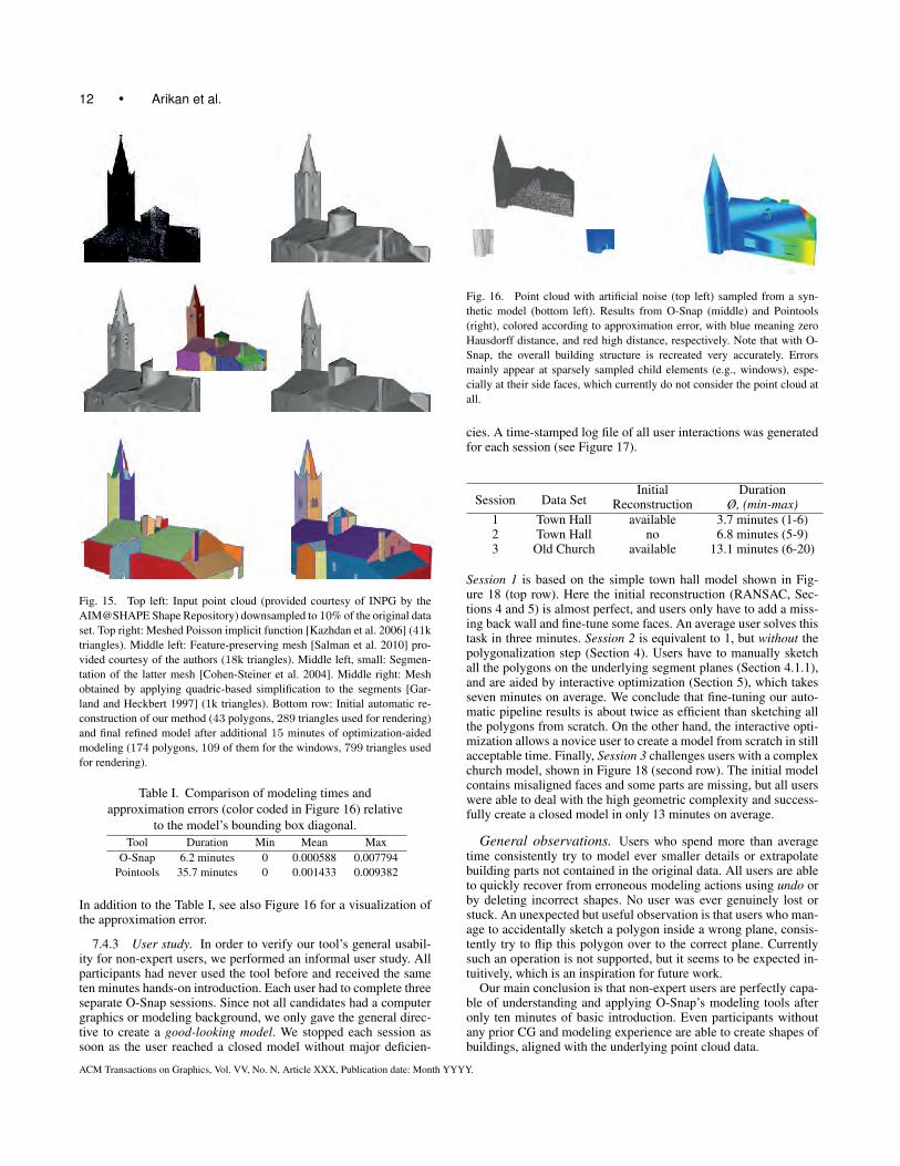
7.4.1 Comparison with meshing methods. To evaluate the vi-sual quality of our reconstructions, we applied our method and var-ious other meshing techniques to the laser scan of the Church ofLans le Villard (Figure 15 top left). Figure 15 compares the dif-ferent approaches: MeshLab’s [2008] implementation of PoissonSurface Reconstruction [Kazhdan et al. 2006] (top right), Salmanet al.’s feature-preserving mesh generation [2010] (middle left),the latter method followed by Graphite’s [2010] implementationof geometry segmentation [Cohen-Steiner et al. 2004] (middle left,small image), and the same model with quadric-based mesh deci-mation [Garland and Heckbert 1997] applied to each segment withfixed boundary, for which we used MeshLab [2008] again (middleright). The third row shows the results of our reconstruction andmodeling pipeline.

7.4.2 Accuracy comparison. We used our system and a com-mercial point-based modeling tool, the Pointools plugin forSketchUp [2011], on a point cloud sampled from a synthetic housemodel. Noise was added to sample positions in the amount of 0.5%of the bounding box diagonal. Modeling was performed by a skilledartist, who was instructed to create the most accurate model possi-ble in the two tools, both of which he had used before. There wereno time constraints. After completion the artist reported to be con-fident having created perfectly accurate models in both tools, butalso that he needed considerably more time and patience for mod-eling in Pointools. In order to quantify this feedback, we comparedHausdorff distances for each result to the original synthetic model(measured using the Metro tool [Cignoni et al. 1996]), and model-ing times (see Table I). The results indicate that our method outper-forms the commercial tool in terms of accuracy and modeling time.



Fig. 15. Top left: Input point cloud (provided courtesy of INPG by theAIM@SHAPE Shape Repository) downsampled to 10% of the original dataset. Top right: Meshed Poisson implicit function [Kazhdan et al. 2006] (41ktriangles). Middle left: Feature-preserving mesh [Salman et al. 2010] pro-vided courtesy of the authors (18k triangles). Middle left, small: Segmen-tation of the latter mesh [Cohen-Steiner et al. 2004]. Middle right: Meshobtained by applying quadric-based simplification to the segments [Gar-land and Heckbert 1997] (1k triangles). Bottom row: Initial automatic re-construction of our method (43 polygons, 289 triangles used for rendering)and final refined model after additional 15 minutes of optimization-aidedmodeling (174 polygons, 109 of them for the windows, 799 triangles usedfor rendering).

Table I. Comparison of modeling times andapproximation errors (color coded in Figure 16) relative

to the model’s bounding box diagonal.Tool Duration Min Mean Max

O-Snap 6.2 minutes 0 0.000588 0.007794Pointools 35.7 minutes 0 0.001433 0.009382

In addition to the Table I, see also Figure 16 for a visualization ofthe approximation error.

7.4.3 User study. In order to verify our tool’s general usabil-ity for non-expert users, we performed an informal user study. Allparticipants had never used the tool before and received the sameten minutes hands-on introduction. Each user had to complete threeseparate O-Snap sessions. Since not all candidates had a computergraphics or modeling background, we only gave the general direc-tive to create a good-looking model. We stopped each session assoon as the user reached a closed model without major deficien-

Fig. 16. Point cloud with artificial noise (top left) sampled from a syn-thetic model (bottom left). Results from O-Snap (middle) and Pointools(right), colored according to approximation error, with blue meaning zeroHausdorff distance, and red high distance, respectively. Note that with O-Snap, the overall building structure is recreated very accurately. Errorsmainly appear at sparsely sampled child elements (e.g., windows), espe-cially at their side faces, which currently do not consider the point cloud atall.

cies. A time-stamped log file of all user interactions was generatedfor each session (see Figure 17).

Session Data SetInitial Duration

Reconstruction Ø, (min-max)1 Town Hall available 3.7 minutes (1-6)2 Town Hall no 6.8 minutes (5-9)3 Old Church available 13.1 minutes (6-20)

Session 1 is based on the simple town hall model shown in Fig-ure 18 (top row). Here the initial reconstruction (RANSAC, Sec-tions 4 and 5) is almost perfect, and users only have to add a miss-ing back wall and fine-tune some faces. An average user solves thistask in three minutes. Session 2 is equivalent to 1, but without thepolygonalization step (Section 4). Users have to manually sketchall the polygons on the underlying segment planes (Section 4.1.1),and are aided by interactive optimization (Section 5), which takesseven minutes on average. We conclude that fine-tuning our auto-matic pipeline results is about twice as efficient than sketching allthe polygons from scratch. On the other hand, the interactive opti-mization allows a novice user to create a model from scratch in stillacceptable time. Finally, Session 3 challenges users with a complexchurch model, shown in Figure 18 (second row). The initial modelcontains misaligned faces and some parts are missing, but all userswere able to deal with the high geometric complexity and success-fully create a closed model in only 13 minutes on average.

General observations. Users who spend more than averagetime consistently try to model ever smaller details or extrapolatebuilding parts not contained in the original data. All users are ableto quickly recover from erroneous modeling actions using undo orby deleting incorrect shapes. No user was ever genuinely lost orstuck. An unexpected but useful observation is that users who man-age to accidentally sketch a polygon inside a wrong plane, consis-tently try to flip this polygon over to the correct plane. Currentlysuch an operation is not supported, but it seems to be expected in-tuitively, which is an inspiration for future work.

Our main conclusion is that non-expert users are perfectly capa-ble of understanding and applying O-Snap’s modeling tools afteronly ten minutes of basic introduction. Even participants withoutany prior CG and modeling experience are able to create shapes ofbuildings, aligned with the underlying point cloud data.


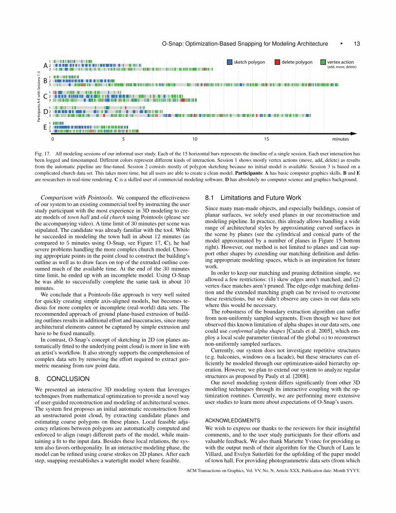
O-Snap: Optimization-Based Snapping for Modeling Architecture • 13Pa

rtic

ipan

ts A

-E w

ith S

essi

ons

1-3

0

delete polygon vertex action(add, move, delete)

sketch polygon

minutes105 15

E

D

C

B

A1

32

1

32

1

32

1

32

1

32

Fig. 17. All modeling sessions of our informal user study. Each of the 15 horizontal bars represents the timeline of a single session. Each user interaction hasbeen logged and timestamped. Different colors represent different kinds of interaction. Session 1 shows mostly vertex actions (move, add, delete) as resultsfrom the automatic pipeline are fine-tuned. Session 2 consists mostly of polygon sketching because no initial model is available. Session 3 is based on acomplicated church data set. This takes more time, but all users are able to create a clean model. Participants: A has basic computer graphics skills. B and Eare researchers in real-time rendering. C is a skilled user of commercial modeling software. D has absolutely no computer science and graphics background.

Comparison with Pointools. We compared the effectivenessof our system to an existing commercial tool by instructing the userstudy participant with the most experience in 3D modeling to cre-ate models of town hall and old church using Pointools (please seethe accompanying video). A time limit of 30 minutes per scene wasstipulated. The candidate was already familiar with the tool. Whilehe succeeded in modeling the town hall in about 12 minutes (ascompared to 5 minutes using O-Snap, see Figure 17, C), he hadsevere problems handling the more complex church model. Choos-ing appropriate points in the point cloud to construct the building’soutline as well as to draw faces on top of the extruded outline con-sumed much of the available time. At the end of the 30 minutestime limit, he ended up with an incomplete model. Using O-Snaphe was able to successfully complete the same task in about 10minutes.

We conclude that a Pointools-like approach is very well suitedfor quickly creating simple axis-aligned models, but becomes te-dious for more complex or incomplete (real-world) data sets. Therecommended approach of ground plane-based extrusion of build-ing outlines results in additional effort and inaccuracies, since manyarchitectural elements cannot be captured by simple extrusion andhave to be fixed manually.

In contrast, O-Snap’s concept of sketching in 2D (on planes au-tomatically fitted to the underlying point cloud) is more in line withan artist’s workflow. It also strongly supports the comprehension ofcomplex data sets by removing the effort required to extract geo-metric meaning from raw point data.

8. CONCLUSION

We presented an interactive 3D modeling system that leveragestechniques from mathematical optimization to provide a novel wayof user-guided reconstruction and modeling of architectural scenes.The system first proposes an initial automatic reconstruction froman unstructured point cloud, by extracting candidate planes andestimating coarse polygons on these planes. Local feasible adja-cency relations between polygons are automatically computed andenforced to align (snap) different parts of the model, while main-taining a fit to the input data. Besides these local relations, the sys-tem also favors orthogonality. In an interactive modeling phase, themodel can be refined using coarse strokes on 2D planes. After eachstep, snapping reestablishes a watertight model where feasible.

8.1 Limitations and Future Work

Since many man-made objects, and especially buildings, consist ofplanar surfaces, we solely used planes in our reconstruction andmodeling pipeline. In practice, this already allows handling a widerange of architectural styles by approximating curved surfaces inthe scene by planes (see the cylindrical and conical parts of themodel approximated by a number of planes in Figure 15 bottomright). However, our method is not limited to planes and can sup-port other shapes by extending our matching definition and defin-ing appropriate modeling spaces, which is an inspiration for futurework.

In order to keep our matching and pruning definition simple, weallowed a few restrictions: (1) skew edges aren’t matched, and (2)vertex-face matches aren’t pruned. The edge-edge matching defini-tion and the extended matching graph can be revised to overcomethese restrictions, but we didn’t observe any cases in our data setswhere this would be necessary.

The robustness of the boundary extraction algorithm can sufferfrom non-uniformly sampled segments. Even though we have notobserved this known limitation of alpha shapes in our data sets, onecould use conformal alpha shapes [Cazals et al. 2005], which em-ploy a local scale parameter (instead of the global α) to reconstructnon-uniformly sampled surfaces.

Currently, our system does not investigate repetitive structures(e.g. balconies, windows on a facade), but these structures can ef-ficiently be modeled through our optimization-aided hierarchy op-eration. However, we plan to extend our system to analyze regularstructures as proposed by Pauly et al. [2008].

Our novel modeling system differs significantly from other 3Dmodeling techniques through its interactive coupling with the op-timization routines. Currently, we are performing more extensiveuser studies to learn more about expectations of O-Snap’s users.

ACKNOWLEDGMENTSWe wish to express our thanks to the reviewers for their insightfulcomments, and to the user study participants for their efforts andvaluable feedback. We also thank Mariette Yvinec for providing uswith the output mesh of their algorithm for the Church of Lans leVillard, and Evelyn Sutterluti for the upfolding of the paper modelof town hall. For providing photogrammetric data sets (from which



Fig. 18. Results from five point cloud data sets (generated from photos) shown from top to bottom: town hall, old church (Photos courtesy of RainerBrechtken), mountain house (Photos courtesy of Sinha et al. [2008]), castle-P19 (Photos courtesy of Strecha et al. [2008]) and playhouse (Photos courtesyof Sinha et al. [2008]). Left to right: input point cloud, initial automatic reconstruction, refined model, final model with advanced details added, final tex-tured model (with the photos simply back-projected onto the model, more sophisticated methods for seamless texturing exist, e.g., Sinha et al.’s graph-cutoptimization [2008]).

we generated the data sets used in the paper), we thank SudiptaSinha (mountain house, playhouse), Rainer Brechtken (old church)and Strecha et al. [2008] (castle-P19). We also acknowledge theAim@Shape Shape Repository for the laser scan of the Church ofLans le Villard.

This work was partially supported by the Austrian Research Pro-motion Agency (FFG) through the FIT-IT project “Terapoints”,project no. 825842. The competence center VRVis is funded byBMVIT, BMWFJ, and City of Vienna (ZIT) within the scope ofCOMET – Competence Centers for Excellent Technologies. Theprogram COMET is managed by FFG.

REFERENCES

ALLIEZ, P., COHEN-STEINER, D., TONG, Y., AND DESBRUN, M. 2007.Voronoi-based variational reconstruction of unoriented point sets. In Pro-ceedings of the fifth Eurographics symposium on Geometry processing.Eurographics Association, Aire-la-Ville, Switzerland, Switzerland, 39–48.

ATKINSON, A. C. AND RIANI, M. 2000. Robust Diagnostic RegressionAnalysis. Springer-Verlag.

AVRON, H., SHARF, A., GREIF, C., AND COHEN-OR, D. 2010. `1-sparsereconstruction of sharp point set surfaces. ACM Trans. Graph. 29, 135:1–135:12.

BOISSONNAT, J.-D. AND OUDOT, S. 2005. Provably good sampling andmeshing of surfaces. Graph. Models 67, 405–451.

BOTSCH, M., PAULY, M., GROSS, M., AND KOBBELT, L. 2006. Primo:coupled prisms for intuitive surface modeling. In Proceedings of thefourth Eurographics symposium on Geometry processing. 11–20.

CAZALS, F., GIESEN, J., PAULY, M., AND ZOMORODIAN, A. 2005. Con-formal alpha shapes. Proceedings Eurographics/IEEE VGTC SymposiumPoint-Based Graphics 0, 55–61.

CHEN, J. AND CHEN, B. 2008. Architectural modeling from sparselyscanned range data. IJCV 78, 2-3, 223–236.

CIGNONI, P., CORSINI, M., AND RANZUGLIA, G. 2008. Meshlab: anopen-source 3d mesh processing system.

CIGNONI, P., ROCCHINI, C., AND SCOPIGNO, R. 1996. Metro: measuringerror on simplified surfaces. Tech. rep., Paris, France.

COHEN-STEINER, D., ALLIEZ, P., AND DESBRUN, M. 2004. Variationalshape approximation. ACM Trans. Graph. 23, 905–914.

DAVIS, T. A. 2011. Algorithm 915, SuiteSparseQR: Multifrontal multi-threaded rank-revealing sparse QR factorization. ACM Transactions onMathematical Software 38, 1.

DEBEVEC, P. E., TAYLOR, C. J., AND MALIK, J. 1996. Modeling andrendering architecture from photographs: a hybrid geometry- and image-based approach. In Proceedings of SIGGRAPH 96. 11–20.



DEMAINE, E. AND O’ROURKE, J. 2007. Geometric Folding Algorithms:Linkages, Origami, Polyhedra. Cambridge University Press.

EDELSBRUNNER, H. AND MUCKE, E. P. 1994. Three-dimensional alphashapes. ACM Trans. Graph. 13, 43–72.

FLEISHMAN, S., COHEN-OR, D., AND SILVA, C. T. 2005. Robust movingleast-squares fitting with sharp features. ACM Trans. Graph. 24, 544–552.

FURUKAWA, Y., CURLESS, B., SEITZ, S. M., AND SZELISKI, R. 2009.Manhattan-world stereo. In IEEE Conference on Computer Vision andPattern Recognition (2009). 1422–1429.

GAL, R., SORKINE, O., MITRA, N. J., AND COHEN-OR, D. 2009.iWIRES: An analyze-and-edit approach to shape manipulation. ACMTransactions on Graphics (Siggraph) 28, 3, #33, 1–10.

GARLAND, M. AND HECKBERT, P. S. 1997. Surface simplification usingquadric error metrics. In Proceedings of the 24th annual conference onComputer graphics and interactive techniques. SIGGRAPH ’97. ACMPress/Addison-Wesley Publishing Co., New York, NY, USA, 209–216.

GRAPHITE. 2010. http://alice.loria.fr/index.php/software.

html.JOLLIFFE, I. T. 2002. Principal Component Analysis, 2nd ed. Springer,

New York.KAZHDAN, M., BOLITHO, M., AND HOPPE, H. 2006. Poisson surface

reconstruction. In Proceedings of the fourth Eurographics symposium onGeometry processing. SGP ’06. Eurographics Association, Aire-la-Ville,Switzerland, Switzerland, 61–70.

KELLEY, C. T. 1999. Iterative Methods for Optimization. Society forIndustrial and Applied Mathematics, Philadephia, PA.

KILIAN, M., FLORY, S., CHEN, Z., MITRA, N. J., SHEFFER, A., AND

POTTMANN, H. 2008. Curved folding. ACM Transactions on Graph-ics 27, 3, #75, 1–9.

KOBBELT, L. P., BOTSCH, M., SCHWANECKE, U., AND SEIDEL, H.-P.2001. Feature sensitive surface extraction from volume data. In Proceed-ings of the 28th annual conference on Computer graphics and interactivetechniques. SIGGRAPH ’01. ACM, New York, NY, USA, 57–66.

LI, Y., WU, X., CHRYSANTHOU, Y., SHARF, A., COHEN-OR, D., AND

MITRA, N. J. 2011. GlobFit: Consistently fitting primitives by discover-ing global relations. ACM Transactions on Graphics 30, 4, to appear.

MUSIALSKI, P., WONKA, P., ALIAGA, D. G., WIMMER, M., VAN GOOL,L., AND PURGATHOFER, W. 2012. A Survey of Urban Reconstruction.In EUROGRAPHICS 2012 State of the Art Reports. Eurographics Asso-ciation, 1–28.

NAN, L., SHARF, A., ZHANG, H., COHEN-OR, D., AND CHEN, B. 2010.SmartBoxes for interactive urban reconstruction. ACM Trans. Graph. 29,93:1–93:10.

PAULY, M., MITRA, N. J., WALLNER, J., POTTMANN, H., AND GUIBAS,L. 2008. Discovering structural regularity in 3D geometry. ACM Trans-actions on Graphics 27, 3, #43, 1–11.

POINTOOLS LTD. 2011. Pointools plugin for sketchup. http://www.

pointools.com/pointools-plug-in-for-sketchup.php.POTTMANN, H., HUANG, Q.-X., YANG, Y.-L., AND HU, S.-M. 2006.

Geometry and convergence analysis of algorithms for registration of 3Dshapes. Int. J. Comput. Vision 67, 277–296.

ROUSSEEUW, P. J. AND LEROY, A. M. 1987. Robust regression and outlierdetection. John Wiley & Sons, Inc., New York, NY, USA.

SALMAN, N., YVINEC, M., AND MERIGOT, Q. 2010. Feature preservingmesh generation from 3D point clouds. Computer Graphics Forum 29, 5,1623–1632.

SCHINDLER, K. AND BAUER, J. 2003. A model-based method for buildingreconstruction. In Proceedings of the First IEEE International Workshopon Higher-Level Knowledge in 3D Modeling and Motion Analysis. 74–82.

SCHNABEL, R., DEGENER, P., AND KLEIN, R. 2009. Completion andreconstruction with primitive shapes. Computer Graphics Forum (Proc.of Eurographics) 28, 2 (Mar.), 503–512.

SCHNABEL, R., WAHL, R., AND KLEIN, R. 2007. Efficient RANSAC forpoint-cloud shape detection. Computer Graphics Forum 26, 2, 214–226.

SINHA, S. N., STEEDLY, D., SZELISKI, R., AGRAWALA, M., AND

POLLEFEYS, M. 2008. Interactive 3D architectural modeling from un-ordered photo collections. ACM Trans. Graph. 27, 159:1–159:10.

STRECHA, C., VON HANSEN, W., GOOL, L. J. V., FUA, P., AND THOEN-NESSEN, U. 2008. On benchmarking camera calibration and multi-viewstereo for high resolution imagery. In CVPR.

VAN DEN HENGEL, A., DICK, A., THORMAHLEN, T., WARD, B., AND

TORR, P. H. S. 2007. VideoTrace: rapid interactive scene modellingfrom video. ACM Trans. Graph. 26.

VANEGAS, C. A., ALIAGA, D. G., AND BENES, B. 2010. Building recon-struction using Manhattan-world grammars. In CVPR. 358–365.

WERNER, T. AND ZISSERMAN, A. 2002. New techniques for automatedarchitectural reconstruction from photographs. In Proceedings of ECCV2002. 541–555.


Documents

O-Snap: Optimization-Based Snapping for Modeling …