O ptimum L ocation of DG U nits C onsidering O peration C ... · losses, distributed generation units have been spread out in the power distribution systems. In the literature review,

International Journal of Computer Applications Technology and Research

Volume 7–Issue 09, 370-375, 2018, ISSN:-2319–8656

www.ijcat.com 370

Optimum Location of DG Units Considering Operation Conditions

Soheil Dolatiary

Islamic Azad University

Central of Tehran,

Tehran, Iran.

Javad Rahmani

Digital electronics Engineering

Islamic Azad University

Science and Research Branch

Tehran, Iran.

Zahra Khalilzad

Digital electronics department,

Shahed university of Tehran

Tehran, Iran.

Abstract: The optimal sizing and placement of Distributed Generation units (DG) are becoming very attractive to researchers these

days. In this paper a two stage approach has been used for allocation and sizing of DGs in distribution system with time varying load

model. The strategic placement of DGs can help in reducing energy losses and improving voltage profile. The proposed work

discusses time varying loads that can be useful for selecting the location and optimizing DG operation. The method has the potential to

be used for integrating the available DGs by identifying the best locations in a power system. The proposed method has been

demonstrated on 9-bus test system.

Keywords: Distribution Generation (DG), Optimal placement, Time-varying load, Load profile, Energy losses

1. INTRODUCTION In the restructured power systems, in order to considering

losses, distributed generation units have been spread out in the

power distribution systems. In the literature review, DG is a

small scale power generation that is usually connected to a

distribution system. DGs mainly consist of renewable energy

resources such as photovoltaics (PV), wind turbines, and fuel

cells. Among them PVs and fuel cells are DC resources and

they are connecting to the power grid by DC/DC and DC/AC

converters. DC/DC converters are mainly used to provide a

controlled output voltage under different load variation [1].

The term DG also implies the use of generation units to lower

the cost of services. A potential advantage of DG over

conventional generations is that the energy production takes

place near the consumer, which can minimize the power

losses in the distribution lines.

Naresh Acharya et al suggested a heuristic method in [2] to

select appropriate location and to calculate DG size for

minimum real power losses. Though the method is effective in

selecting location, it requires more computational efforts. The

optimal value of DG for minimum system losses is calculated

at each bus. Placing the calculated DG size for the buses one

by one, corresponding system losses are calculated and

compared to decide the appropriate location. Moreover, the

heuristic search requires exhaustive search for all possible

locations which may not be applicable to more than one DG.

This method is used to calculate DG size based on

approximate loss formula may lead to an inappropriate

solution [3].

Go swami et al, [4] have analyzed load voltage sensitivity

considering load models of voltage dependent load, whereas

this method has been done by genetic algorithm. Singh et al

[5] unlike other studies which dealt with the constant load

models have studied on the effect of different load and

sensitive to voltage and frequency and then they found the

best location for DG units.

Authors of [6] have used and analytical method for optimal

DG allocation, this method is based on power flow for the

radial network and calculate loss sensitivity factor and priority

list, which causes reduction on the search space. In [7] are

proposed a heuristic method for optimal sizing and placement

of DG in order to reduce economic costs, like energy cost,

investment, operational cost, loss cost and technical aspect

such as energy loss and voltage level.

In [8] optimal DG location is obtained considering economic

and operational limits of DG and distribution system. Optimal

DG placement is accomplished in [9] to maximize DG

application benefit and minimize the costs for both utility and

customers. A loss minimization approach is used in [10] too

find optimal DG location.

There are so many DG placement methods in hand though

each of these methods only focuses on some parameters. The

optimal DG placement defined in [11] takes reliability, loss

reduction, and load prediction into account while it fails to

account for other parameters such as productivity, cost

effectiveness, and type of DG. The optimal DG placement

defined in [12] takes productivity, cost, effectiveness, loss

reduction, and reliability and DG type into account and fails

to consider other parameters.

In [13], a Newton-Raphson algorithm based load flow

program is used to solve the load flow problem. The

methodology for optimal placement of only one DG type 1 is

proposed. Moreover, the heuristic search requires exhaustive

search for all possible locations which may not be applicable

to more than one DG. Therefore, in this paper, PSO method is

proposed to determine the optimal location and sizes of multi-

DGs to minimize total real power loss of distribution systems.

Whether DG is properly planned and operated it may provide

benefits to distribution networks (e.g., reduction of power

losses and/or deferment of investments for network enforcing,

etc.), otherwise it can cause degradation of power quality,

reliability, and control of the power system [14]. Also,

placement of different DG units in the power system should



www.ijcat.com 371

be done considering interactions of the different units under

primary and secondary frequency regulation carefully to

prevent power system instability [15]. Thus, DG offers an

alternative that planners should explore in their search for the

best solution to electric supply problems and requires new

planning paradigms and procedures able to face a more

complex and uncertain scenario [16], [17], [18], [19].

Ault et al. in [20] have pointed out the dichotomy between the

advanced status of academic researches on planning and the

unwillingness of companies to resort to such algorithms.

Indeed, the planners need tools to deal with uncertainties,

risks, and multiple criteria. The final choice will be

subjectively operated in the set of good solutions. To consider

uncertainties of parameters and system inputs, [21] uses

reachability analysis which is a mathematical analysis based

on uncertain matrices. Reachability analysis can also be used

to study DG integration and planning uncertainties.

An optimization technique should be employed for the design

of engineering systems, allowing for the best allocation of

limited financial resources. In electric power systems, most of

the electrical energy losses occur in the distribution systems.

It is a tool that can be used both for the design of a new

distribution system and for the resizing of an existing system

[22]. In [23] application of robust MPC provides an optimal

solution to handle the system uncertainties. In [24] Monte-

Carlo method is used to take uncertainties into account for

renewable generation.

Distributed generation is not limited to conventional

generation of electricity. A controlled reduction in demand

can play the same role as distributed generation. For instance,

[25] studies the possibility of using aggregation of small

{ON/OFF} loads as a compensation for renewables variations.

It was shown that only in Texas, 1.5 GW of flexible demand

can act as distributed generation when controlled over the

WiFi network.

Distributed Generation sometimes provides the most

economical solution to load variations. Under voltages or

overloads that are created by load growth may only exist on

the circuit for a small number of hours per day or/ month or/

year. There may be many locations where DGs can be located

and provide the necessary control [26]. Also, the authors

address this issue for small size distributed generators in [27].

In [28] UPFC acts like a DG, and leads to power swing

reduction and enhancing the system stability by reactive

power injection.

However, the current research lacks the complete solution to

the determination of DG allocation and operation, together

with considering load voltage profile and time varying loads.

For example too much emphasis on power loss cost and

construction expenses but ignorance of the time varying loads

and energy loss factors.

Moreover, the absence of the consideration about operation of

DGs in the network structure may lead to the confusion of the

benefit of placing DGs and dispatching policy.

The optimal placement and dispatching investigated in this

paper are divided into two major parts, namely optimal

allocation and optimal sizing of DGs. In firs part of section 2,

placement of DGs is done based on the summation of energy

losses during 24 hour and for time varying loads. In second

part of section 2 sizing of DGs is determined in each time

interval. In section 3 simulation network is explained.

Simulation results on the test system are illustrated in section

4. Then the conclusion is given in section 5.

2. PROPOSED METHOD

2.1 Optimal Allocation of DGs Optimal DG placement achieved to gain the optimal DG

location to minimize or maximize a particular objective

function. The optimal allocation model of DG is used to solve

the problem of sizing and siting of various DGs [29,30].

Here, an energy based approach is explained for placement of

a conventional DG in a distribution system. In this work

conventional DGs are supposed to be diesel generators and

fossil fuels producers. Wind turbines and solar panels have

some limitations that cannot be used everywhere in

distribution network and should be place in some particular

locations. By considering these facts, only conventional DGs

will be placed.

Loads that are studied here, are time varying that have

different values at each time of day and night. Thus, the goal

is minimizing the energy loss of distribution network. Load

model are usually considered to be constant in a time period,

while in reality, loads are function of the ambient temperature

and human behavior [31,32]

So, considering energy losses instead of power losses seems

better and therefore, minimizing the energy losses is the final

goal. Using medium-voltage and high-voltage dc collection

system would further improve the efficiency [33]. In [34] and

[35], a new method for application in communication circuit

system is proposed that it causes increasing the efficiency,

PAE, output power and gain.

In order to minimizing the energy losses, load modeling is

inevitable. As the load varies along time in 24 hour of a day,

the time period should be divided into some appropriate

intervals in order to approximate the load to be constant in

each interval based on load profile. For instance, load profile

in 24 hours is considered as follows:

Figure 1: Load profile in 24 hours

Considering magnitude and variation of load during 24 hours

of a day, sometime-intervals seem appropriate for the

proposed method. Depending on the accuracy needed in a



www.ijcat.com 372

power network, the number of time intervals are computed. In

each interval, load is being estimated by the average of load

during at that interval with trapezoid method.

It should be noted that the duration of time intervals should

not be the same. For example in the first times of a day that

the demands are low and the variation is low enough to be

neglected, the duration of that interval could be large enough

to estimate the load at that interval. Although, in peak hours

the variation of demands are high and the time interval should

be considered small.

Here, in each interval in order to reduce energy losses of total

network, the generation energy of each bus is computed. The

proposed energy loss factor due to line currents can be defined

as:

Where:

Rk are the kth line total resistance.

N is the number of lines in the network.

T is the number of intervals for load modeling.

Ikj is the current for kth line in jth interval.

tj is the duration of kth interval.

With this in mind, the optimization objective and the

constraints are as follows:

Where, and

In this section, the goal is siting the DGs in special buses in

order to minimizing the energy loss. For this purpose, it is

assumed that in each bus of the network, there is possibility to

generate electrical energy and so, DGs could be place

anywhere in the power network.

Power generated in each interval by each DG could be

varying from 0 MW to the total load at that interval. The step

of variation is considered 2 MW. In other words, DGs are

available at sizes of 2 MW and in each bus, there is possibility

to place any number of DGs.

The result of optimizing this problem is the power generated

by each DG at each interval. The output power of each DG is

given by:

Where, Kij is the number of 2 MW steps in ith bus and jth time

interval. The total energy produced by each bus during the 24

hours is as follows:

As there is limitation in producing energy at all buses,

selecting the buses that generate more energy is important.

Therefore, by selecting the buses with bigger Ei and based on

the number of buses needed for generating energy, placement

of DGs is finished. For example if just 4 buses have this

ability to be placed by DGs, 4 buses with higher total energy

producing will be selected.

2.2 Optimal Sizing of DGs In this section, after optimal DG placement and selecting the

generator buses, the power generated by each DG in the

selected buses for each time interval should be determined. In

other words, Operation of DGs contributes in minimizing the

total energy losses of the network. Thus, scheduling the

energy produced by each DG should be done.

For this purpose, the minimizing objective is as mentioned

before. The difference is just the number of buses producing

energy. In the previous section, the placement of DGs is done

in all the buses of the network and based on the total energy

produced in each bus, buses with higher Ei was selected. In

this section, placement of DGs is just done in the selected

buses of the previous section.

In optimizing the size of the DGs in order to improve

computational accuracy, steps of variation in the power

generated is considered 0.5 MW. In other words, DGs are

available at sizes of 0.5 MW and in each bus, there is

possibility to place any number of DGs. It should be

considered that increasing the steps of variation is possible,

due to reduction in the number of buses generating energy and

so the computational time will not increase so much.

With this consideration, the objective function and

optimization problem is as mentioned before. The difference

is just the output. The output of this optimization is generated

power matrix in each bus.

The matrix is as follows:

Where Pij is the generated power of ith bus producer energy

and time interval and is computed as follows:

In this formula, Kij is the number of 0.5 MW steps.

According to this goal optimization, the loss reduces when

DGs are placed. Also, the voltage limits that mentioned

before, shows that the appropriate voltage of a certain bus

depends on the minimum and maximum voltages of the bus

which considered 0.95 and 1.05 p.u, respectively.



www.ijcat.com 373

3. SIMULATION NETWORK In the proposed work, in order to implement the suggested

method and compare the results with the network without

DGs, a 9-bus distribution ring network has been selected as a

sample. It should be noted that the specified algorithm can be

used for all distribution networks with any number of buses

and there is no limitation in implementing this algorithm. The

single line diagram of the sample network is illustrated in

figure 2.

Figure 2: Single line diagram of the sample network

According to figure 2, the nine-bus system contains two

sections. Section 1 is buses 1, 2, and 3 with voltage of 63 kV.

These buses get connected to the other section by

transformers with the ratio of 63/20. The other section is

buses 4 to 9 with voltage of 20 kV. Placement of DGs is done

in section 2, in the ring network with buses of 20 kV.

Table 1 shows the data of the lines of the network.

Table 1: Data of the lines of the network

Line R (pu) X (pu)

1 0.01 0.085

2 0.032 0.161

3 0.017 0.092

4 0.039 0.17

5 0.085 0.072

6 0.0119 0.1008

For load modeling, it is considered that the load variation

curve is as plotted in figure 1. So, 7 time interval could be

appropriate for this purpose. These time intervals are as

follows:

Figure 3 shows the load profile estimation for load number 1

in 24 hours of a day.

Figure 3: Load profile

In table 2, data of the loads of the system is shown.

Table 2: Data of loads of the network

Time

interva

l

Load

1

Load

2

Load

3

Load

4

Load

5

Load

6

0-5 2 2 1 0.5 1.2 1

5-7 2.5 2 1.2 1 1.5 1.1

7-12 3.2 2.7 1.8 1.5 2 1.4

12-16 2.6 2.1 1.2 0.9 1.4 1.2

16-20 5 4 3 3 3 2

20-22 4 3.5 2.7 2.8 3 1.8

22-24 2.5 2.1 1.3 1.1 1.4 1.5

4. SIMULATION RESULTS This study aims to optimize the placement and operation of

DGs by taking energy losses into account. It should be noted

that siting the DGs is done in 20 kV buses.

The peak demand in this network is 20 MW. Thus, the

maximum total power generated by these 3-DG, are

considered to be nearly 20 MW in peak hours. In other time

intervals, also the total energy produced by DGs is near the

total load at that interval.

In the first step, the goal is the placement of DGs in the

network. By implementing the proposed method on the

sample network, these results are achieved.

In this case, it is assumed that only 3 buses can produce

energy. By this consideration, buses 1, 5 and 6 which have the

biggest Ei are selected.

In the second step, the goal is optimal operation of DGs in the

selected buses. Here, the algorithm of sizing the DGs is

implemented on the buses 1, 5 and 6.

The following matrix is achieved for power generated at each

time interval.



www.ijcat.com 374

Time interval E1 E2 E3

0-5 1.5 2 2

5-7 1.5 2 2

7-12 2 2.5 3

12-16 1.5 2 2.5

16-20 2.5 4 4

20-22 2.5 3.5 3

22-24 1.5 2 2

The above matrix shows that some DGs produce more energy

than the other one in some intervals and in the other intervals

it is vice versa. For example, DG 3 in times 7 to 16 produce

more energy than DG 2, but in times 20 to 22 produce less

energy than DG 2.

By considering the results of the above matrix, it is shown that

placement of the DGs should not be based on the peak

demand which is done in many of the research.

This method schedules the DGs based on the minimization of

energy loss and gives a generating profile to each DG.

Table 3 compares the energy losses of the proposed method

with the case that sizes of DGs are equal. Table 4 compares

the results with other placement of DGs. The results of the

tables show that the proposed method has the optimal

solution.

Table 3: Comparison of the proposed method with equally

dispatch

methods Energy loss(MWh)

Proposed method 14.636

Equally dispatched 20.742

Table 4: Comparison of the proposed method with other

placement of DGs

DG placement at buses Energy loss(MWh)

1,5,6 14.636

1,4,3 17.892

2,4,6 15.465

1,2,5 20.886

2,3,4 22.846

2,5,6 17.632

By considering the results that shown in table 3 and 4, it is

obvious that placement of DGs should not be based on the

peak load, which is done in many of the research.

5. CONCLUSION This paper has discussed a two stage methodology of finding

the optimal location and sizes of DGs for maximum energy

loss reduction of distribution systems. First stage is DG placement method which is proposed to find optimal DG

location. Second stage is optimal DG operation based on load

varying. Voltage constraints are included in the algorithm.

This methodology is tested on 9 bus system. By installing

DGs at all the potential locations and optimizing the size at

each time interval, the total energy loss of the system has been

reduced and the voltage profile of the system is also

considered.

Inclusion of the non-linear loads and power quality constraints

is the future scope of this work.

6. REFERENCES [1] P. M. Shabestari, G. B. Gharehpetian, G. H. Riahy, and S.

Mortazavian, "Voltage controllers for DC-DC boost

converters in discontinuous current mode," International

Energy and Sustainability Conference, Framingdale, NY,

2015, pp. 1-7.

[2] Naresh Acharya, Pukar Mahat, N. Mithulanathan, “An

analytical approach for DG allocation in primary distribution

network”, Electric Power and Energy System, vol. 28.

[3] M. Padma Lalitha, V.C. Veera Reddy, V. Usha, “Optimal

DG placement for minimum real power loss in radial

distribution systems using PSO”, Journal of Theoretical and

Applied Information Technology, pp. 107-116, 2010

[4] R.K. Singh, et al., “Optimal Allocation of Distributed

Generation in Distribution Network with Voltage and

Frequency Dependent Loads,” ICIIS, 2008, pp. 1-5.

[5] R.K. Singh and S.K. Goswami, “Optimal Siting and Sizing

of Distributed Generations in Radial and Networked Systems

Considering Different Voltage Dependent Static Load

Models,” IEEE International Conference on Power and

Energy, 2008, pp. 1535-1540.

[6] P. Alemi and G.B. Gharehpetian, “DG Allocation Using

an Analytical Method to Minimize Losses and to Improve

Voltage Security,” International conference on Power and

Energy, Malaysia, IEEE, 2008, pp. 1575-1580.

[7] C. Tautiva, “Optimal Placement of Distributed Generation

on Distribution Networks,” Universities power engineering

conference, 2009, pp. 1-5.

[8] Rosehart W, Nowicki E, “ Optimal Placement of

Distributed Generation”, Proceeding of 14th Power Systems

ComputationConference section 11, Sevilllaa 2002 ,pp.1-5

[9] Silvestri a, Berrizi A, Buonanno S, “Distributed

Generation Planning Using GA”, IEEE PowerTech, 1999.

[10] Celli G, Pilo F., “Optimal Distributed Generation

Allocation in MV Distribution Networks”, IEEE PES

Conference on Power Industry Computer Applications, 2001.



www.ijcat.com 375

[11] P. P. Barker and R. W. de Mello, “Determining the Im-

pact of Distributed Generation on Power Systems. I. Ra-dial

Distribution Systems,” IEEE Power Engineering So-ciety

Summer Meeting, Seattle, 16-20 July 2000, pp. 1645-1656.

[12] N. Hadisaid, J.-F. Canard and F. Dumas, “Dispersed

Gen-eration Impact on Distribution Networks,” IEEE

Computer Applications in Power, Vol. 12, No. 2, 1999.

[13] Kennedy J and Eberhart R, “Particle Swarm Optimizer,”

IEEE International Conference on Neural Networks (Perth,

Australia), IEEE Service Center Piscataway, NJ, IV,1995.

[14] N. Jenkins, R. Allan, P. Crossley, D. Kirschen, and G.

Strbac, Embedded Generation. London, U.K.: IEE, 2000.

[15] M. Amini and M. Almassalkhi, “Investigating delaysin

frequency-dependent load control,” in InnovativeSmart Grid

Technologies-Asia (ISGT-Asia), 2016 IEEE. IEEE, 2016, pp.

448–453.

[16] P. P. Barker and R.W. de Mello, “Determining the

impact of distributed generation on power systems: Part 1—

Radial distribution systems,” in Proc. IEEE Power Eng. Soc.

Summer Meeting, vol. 3, Seattle, WA, Jul. 16–20, 2000.

[17] R. C. Dugan and S. K. Price, “Issues for distributed

generation in the US,” in Proc. IEEE Power Eng. Soc. Winter

Meeting, vol. 1, New York, Jan. 2002, pp. 121–126.

[18] R. C. Dugan, T. E. McDermott, and G. J. Ball, “Planning

for distributed generation,” IEEE Ind. Appl. Mag, 2001.

[19] G. W. Ault and J. R. McDonald,“Planning for distributed

generation within distribution networks in restructured

electricity markets,”IEEE Power Eng. Rev., 2000.

[20] M. H. Imani, et al., "Simultaneous presence of wind farm

and V2G in security constrained unit commitment problem

considering uncertainty of wind generation," in Texas Power

and Energy Conference (TPEC), 2018, pp. 1-6.

[21] P. M. Shabestari, S. Ziaeinejad and A. Mehrizi-Sani,

"Reachability analysis for a grid-connected voltage-sourced

converter (VSC)," IEEE Applied Power Electronics

Conference and Exposition (APEC), San Antonio, TX,

March, 2018, pp. 2349-2354.

[22] Eduardo G. Carrano, et al., “Electric Distribution

Network Multi objective Design using a Problem Specific

Genetic Algorithm” IEEE Transactions on Power Delivery,

Vol. 21, No. 2, April 2006.

[23] M. Ghanaatian; S. Lotfifard, "Control of Flywheel

Energy Storage Systems in Presence of Uncertainties" IEEE

Transactions on Sustainable Energy, 2018.

[24] S. Jafarishiadeh, M. Farasat “Modeling and Sizing of an

Undersea Energy Storage System”, IEEE Transactions on

Industry Applications, vol. 54, no. 3, pp. 2727-2739, 2018.

[25] M. S. Modarresi, L. Xie, and C. Singh “Reserves from

Controllable Swimming Pool Pumps: Reliability Assessment

and Operational Planning,” in Proc. 51st Hawaii International

Conference on System Sciences (HICSS), January 2018.

[26] N. Ghanbari, H. Mokhtari, S. Bhattacharya, “Optimizing

Operation Indices Considering Different Types of Distributed

Generation in Microgrid Applications”, Energies 2018, 11,

894.

[27] N. Ghanbari, H. Golzari, H. Mokhtari and M. Poshtan,

"Optimum location for operation of small size distributed

generators," IEEE International Conference on Renewable

Energy Research and Applications, CA, 2017, pp. 300-303.

[28] H. Gharibpour, H. Monsef, M. Ghanaatian, "The

comparison of two control methods of power swing reduction

in power system with UPFC compensator" 20th Iranian

Conference on Electrical Engineering (ICEE) 2012.

[29]K. Yousefpour,et al., "Dynamic Approach for Distribution

System Planning Using Particle Swarm Optimization."

International Journal of Control Science and Engineering.

[30] H. Pourgharibshahi, et al., "Verification of computational

optimum tilt angles of a photovoltaic module using an

experimental photovoltaic system," Environmental Progress &

Sustainable Energy, vol. 34, no. 4, pp. 1156-1165, 2015.

[31] M. Amini and M. Almassalkhi, "Trading off robustness

and performance in receding horizon control with uncertain

energy resources," in 2018 Power Systems Computation

Conference (PSCC), 2018, pp. 1-7.

[32] F. Rassaei, W. Soh, K. Chua, and M.S. Modarresi,

“Environmentally-friendly demand response for residential

plug-in electric vehicles”, in Proc. Power and Energy

Conference (TPEC), College Station, TX, 2017.

[33] S. Jafarishiadeh, et al., "Grid-connected operation of

direct-drive wave energy converter by using HVDC line and

undersea storage system" in Proc. Energy Conversion

Congress and Exposition (ECCE), Cincinnati, OH , 2017.

[34] F. Rahmani, F. Razaghian, and A. Kashaninia, "High

Power Two-Stage Class-AB/J Power Amplifier with High

Gain and Efficiency," Journal of Academic and Applied

Studies (JAAS), vol. 4, pp. 56-68, 2014.

[35] F. Rahmani, F. Razaghian, and A. Kashaninia, "Novel

Approach to Design of a Class-EJ Power Amplifier Using

High Power Technology," World Academy of Science,

Engineering and Technology, International Journal of

Electrical, Computer, Energetic, Electronic and

Communication Engineering, vol. 9, pp. 541-546, 2015.



www.ijcat.com 376

Performance Evaluation of VANETs for Evaluating Node

Stability in Dynamic Scenarios

Vani Malagar

Assistant Professor

Model Institute of Engineering

and Technology

Kotbhalwal,India

Manoj Kumar

Assistant Professor

Shri Mata Vaishno Devi

University

Katra, India

Sonakshi Gupta

Assistant Professor

Model Institute of Engineering

and Technology

Kotbhalwal,India

Abstract: Vehicular ad hoc networks (VANETs) are a favorable area of exploration which empowers the interconnection amid the

movable vehicles and between transportable units (vehicles) and road side units (RSU). In Vehicular Ad Hoc Networks (VANETs),

mobile vehicles can be organized into assemblage to promote interconnection links. The assemblage arrangement according to

dimensions and geographical extend has serious influence on attribute of interaction .Vehicular ad hoc networks (VANETs) are

subclass of mobile Ad-hoc network involving more complex mobility patterns. Because of mobility the topology changes very

frequently. This raises a number of technical challenges including the stability of the network .There is a need for assemblage

configuration leading to more stable realistic network. The paper provides investigation of various simulation scenarios in which

cluster using k-means algorithm are generated and their numbers are varied to find the more stable configuration in real scenario of

road.

Keywords: VANET; RSU; Clustering; K-means; CBR; Cluster Head;

1. INTRODUCTION

VANET is the preeminent element in the intelligent transport system (ITS) constitutes with the basic requirements such as the number of nodes that acts as vehicles, embedded OBU i.e. a communication device and RSUs that are considered as the a group of fixed constituents along the road, literally called road side units (RSUs) [1][3]. A vehicle unit that contains OBU has a group of interconnection unit’s linkage that grants the straight connection between the node (vehicles) and RSUs within its vicinity range. In order to connect with other networks for communications such as Internet, RSUs behave as gateway. This system allows the vehicles to warn from collisions, sudden breakage by allowing them to communicate with the movable units and the roadside infrastructures[6].ITS used for traffic management, for retrieving the vehicle owner’s information, check on the mobility of the vehicles, in management of railway services. In ITS speed, position, velocity types of information are communicated [10].

VANETs platforms a broad category of usage in paved surface safety, user preference entertainment, and optimization of mobile trade in conformity to vehicle-to-0vehicle (V2V) and vehicle-to-RSU (V2R) interconnections. Communication is a means through which different components communicate with each other[2].In VANET communication is between different vehicles ,between vehicles and RSU or the vehicle & the RSU .Communication in Vanet can be categorized into various communication patterns such as Vehicle –to-Vehicle (V2V), Vehicle –to –Infrastructure(V2I) and Cluster-to-Cluster[12]. The

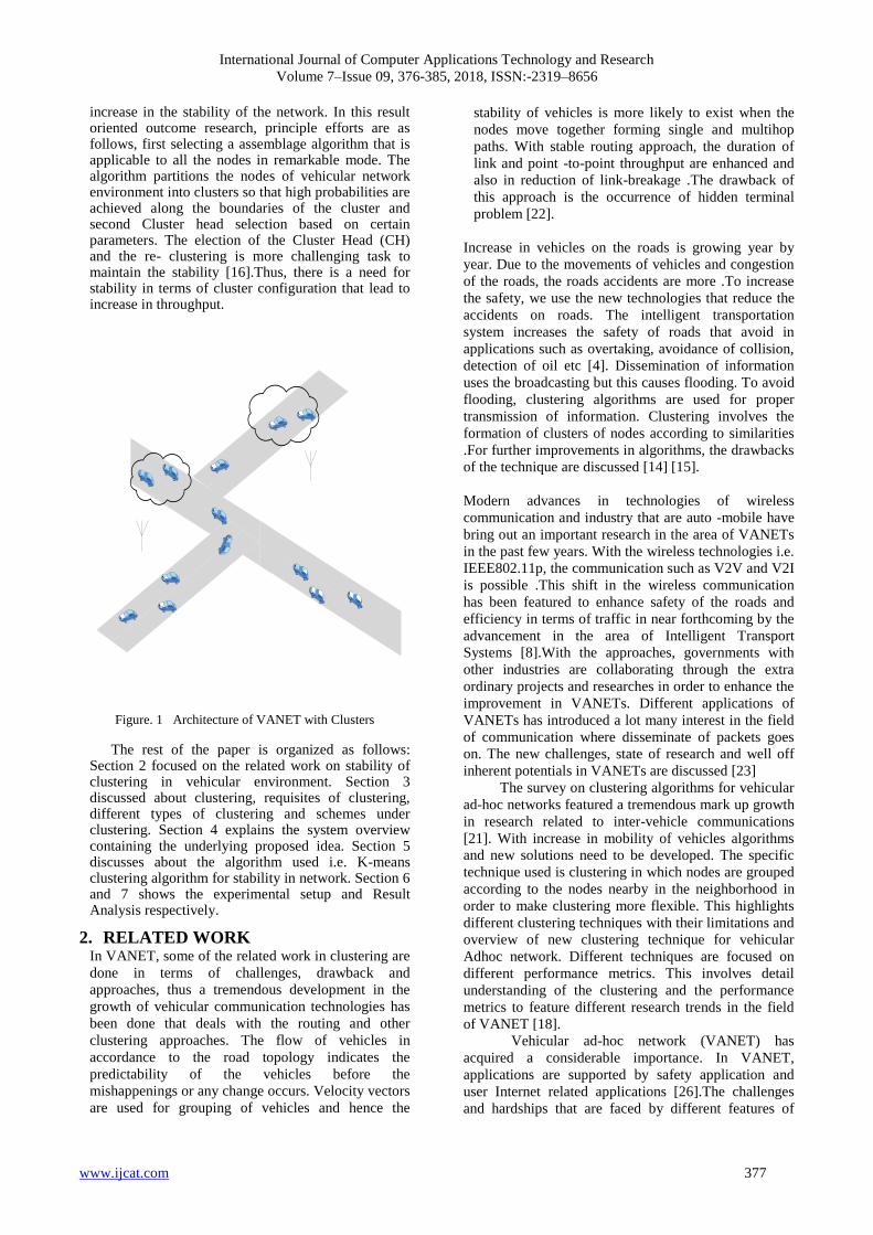
V2V as a type of vehicle to vehicle communication is for cooperative driving .V2I is a type of vehicle to infrastructure communication in which no. of Access points are positioned with the static infrastructures [4][7]. Similarly C2C is the type of cluster to cluster communication in which different vehicles group together forming a self clusters that communicate with other clusters of vehicles as shown in figure 1[3]. The cluster consists of cluster members and the cluster heads for communication. The route of packets within a given range or area using different routing algorithms are used .The establishment of route is significant as links are important for communication between the nodes [27]. Due to the wide range of the mobility, the stability of network is very challenging task.

As per, United States of Federal Communication Commission (USFCC), DSRC has allotted 75-MHz radio spectrum in the 5.9-GHz band for V2V and V2R communication, inspired from the vehicular communication[10][13].The spectrum of the DSRC consists of the control channel and the service channel. The service channel i.e. 6 in no. are considered to be for both types of applications i.e. safety and non-safety. For controlling of information, control channel is used to deliver the priority based safety short messages [5] [11].

According to the Analysis, there is great demand for high throughput that includes in it a great challenge to the safety applications in VANETs as communication are more complex as shown in Figure 1[2][5]. Therefore a clustering approach, deals with the



www.ijcat.com 377

increase in the stability of the network. In this result oriented outcome research, principle efforts are as follows, first selecting a assemblage algorithm that is applicable to all the nodes in remarkable mode. The algorithm partitions the nodes of vehicular network environment into clusters so that high probabilities are achieved along the boundaries of the cluster and second Cluster head selection based on certain parameters. The election of the Cluster Head (CH) and the re- clustering is more challenging task to maintain the stability [16].Thus, there is a need for stability in terms of cluster configuration that lead to increase in throughput.

Figure. 1 Architecture of VANET with Clusters

The rest of the paper is organized as follows: Section 2 focused on the related work on stability of clustering in vehicular environment. Section 3 discussed about clustering, requisites of clustering, different types of clustering and schemes under clustering. Section 4 explains the system overview containing the underlying proposed idea. Section 5 discusses about the algorithm used i.e. K-means clustering algorithm for stability in network. Section 6 and 7 shows the experimental setup and Result Analysis respectively.

2. RELATED WORK In VANET, some of the related work in clustering are

done in terms of challenges, drawback and

approaches, thus a tremendous development in the

growth of vehicular communication technologies has

been done that deals with the routing and other

clustering approaches. The flow of vehicles in

accordance to the road topology indicates the

predictability of the vehicles before the

mishappenings or any change occurs. Velocity vectors

are used for grouping of vehicles and hence the

stability of vehicles is more likely to exist when the

nodes move together forming single and multihop

paths. With stable routing approach, the duration of

link and point -to-point throughput are enhanced and

also in reduction of link-breakage .The drawback of

this approach is the occurrence of hidden terminal

problem [22].

Increase in vehicles on the roads is growing year by

year. Due to the movements of vehicles and congestion

of the roads, the roads accidents are more .To increase

the safety, we use the new technologies that reduce the

accidents on roads. The intelligent transportation

system increases the safety of roads that avoid in

applications such as overtaking, avoidance of collision,

detection of oil etc [4]. Dissemination of information

uses the broadcasting but this causes flooding. To avoid

flooding, clustering algorithms are used for proper

transmission of information. Clustering involves the

formation of clusters of nodes according to similarities

.For further improvements in algorithms, the drawbacks

of the technique are discussed [14] [15].

Modern advances in technologies of wireless

communication and industry that are auto -mobile have

bring out an important research in the area of VANETs

in the past few years. With the wireless technologies i.e.

IEEE802.11p, the communication such as V2V and V2I

is possible .This shift in the wireless communication

has been featured to enhance safety of the roads and

efficiency in terms of traffic in near forthcoming by the

advancement in the area of Intelligent Transport

Systems [8].With the approaches, governments with

other industries are collaborating through the extra

ordinary projects and researches in order to enhance the

improvement in VANETs. Different applications of

VANETs has introduced a lot many interest in the field

of communication where disseminate of packets goes

on. The new challenges, state of research and well off

inherent potentials in VANETs are discussed [23]

The survey on clustering algorithms for vehicular

ad-hoc networks featured a tremendous mark up growth

in research related to inter-vehicle communications

[21]. With increase in mobility of vehicles algorithms

and new solutions need to be developed. The specific

technique used is clustering in which nodes are grouped

according to the nodes nearby in the neighborhood in

order to make clustering more flexible. This highlights

different clustering techniques with their limitations and

overview of new clustering technique for vehicular

Adhoc network. Different techniques are focused on

different performance metrics. This involves detail

understanding of the clustering and the performance

metrics to feature different research trends in the field

of VANET [18].

Vehicular ad-hoc network (VANET) has

acquired a considerable importance. In VANET,

applications are supported by safety application and

user Internet related applications [26].The challenges

and hardships that are faced by different features of



www.ijcat.com 378

VANET such as mobility, quality of service, channel

fading property, and channel competition mechanism

etc on data transmission in VANET. Thus it involves

the clustering and the idea of election of cluster head

with different clustering techniques for transmission of

data. The proposed idea of clustering considers the

difference in the velocities of the nodes in their vicinity,

cluster members and the node degrees in a cluster. The

requirements of QoS of delay and throughput sensitive

service considered by the clustering [17]. Some of the

related work are also discussed.

In DDMAC i.e. distributed multichannel and

mobility aware cluster based MAC protocol aims to

overcome high collision rate and the latency and

increases the high stability. The creation of more stable

cluster is based on the channel scheduling and

mechanism known as adaptive learning in which they

both combine within fuzzy-logic interference system.

The hidden terminal problem eliminated, when each

cluster use different sub channel from its neighbors in

distributed manner [28].

To accomplish stable cluster, node having high

mobility contrasted with its neighboring nodes can't be

chosen as a cluster head. In the event that such a node is

chosen as cluster head, the likelihood of cluster

breakage and even re-grouping is immense.

Subsequently, MOBIC suggests that a node with

slightest versatile nature contrasted with neighboring

nodes ought to be chosen as the cluster head. MOBIC is

fundamentally intended for versatile especially mobile

ad-hoc network works for VANET. It utilizes versatility

metric for determination of cluster heads. It relies on

upon lowest ID algorithms. The clusters framed by

utilizing this technique are more stable when contrasted

with the Lowest-ID algorithm with slightest cluster

head .The rate of cluster head modifications is

decreased by 33 percent when contrasted with the

Lowest-ID clustering algorithm [24]

Zhenxia Zhang et al. review about a novel

clustering plan where clusters are chosen in view of the

relative versatility between vehicles at multi-hop level.

This method utilizes transmission of packet delay in

order to produce distance between two vehicle nodes in

the system. It is acquired from beacon delay on every

node transmitted and reached to different nodes.

Vehicle nodes having low total mobility can be chosen

as the cluster head nodes. In the wake of getting two

beacon messages, the vehicles can ascertain the vehicles

relative mobility. In situations, where two cluster heads

are in same range, the re-clustering of nodes is deferred

for a little measure of time which helps in enhancing

stability of cluster. One of the upsides of this method is

that it stays away from irrelevant re- clustering [25].

3. CLUSTERING IN VANET Clustering or assemblage is the formation of small

groups of nodes known as clusters in order to split the

network. A cluster in VANET elaborates the concept of

the set of nodes in one group and the communication

that takes place between the nodes. The nodes in a

particular cluster elect one Cluster Head (CH) from all

the nodes in a cluster [16] [18].

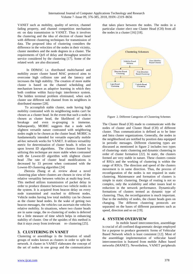
Figure 2. Different Categories of Clustering Schemes

The Cluster Head (CH) made to communicate with the

nodes of cluster and Cluster Head (CH) of different

cluster. Thus communication is defined as to be Inter

and Intra cluster organizations. Generally, the nodes in

the neighborhood are notified by position data equipped

in periodic messages. Different clustering types are

discussed as mentioned in figure 2 includes two types

of clustering- static clustering and dynamic clustering in

order of cluster formation [22]. In static, the clusters

formed are very stable in nature. These clusters consist

of RSUs and the working of clustering is within the

range of RSUs. The direction and speed of the clusters

movement is in same direction. Thus, the process of

reconfiguration of the nodes is not required in static

clustering. Maintenance and formation of clusters is

simple in static clustering. Design of routing is not so

complex, only the scalability and other issues lead to

reduction in the network performance. Dynamically

formations of clusters termed as dynamic type of

clustering. Thus, the reconfiguration is much important.

Due to the mobility of nodes, the cluster heads goes on

changing. The different clustering protocols are

separated on the bases of different parameters such as

speed, direction and so on [19].

4. SYSTEM OVERVIEW In mobile based interconnection, assemblage

is crucial of all confined diagrammatic design employed

for a purpose to produce geometric forms of Vehicular

Based Network which is least consistent [12]. Most of

the assemblage implementation of vehicular based

interconnection is featured from mobile Adhoc based

networks (MANET). Nevertheless, VANET peripherals



www.ijcat.com 379

are represented by their considerable distinguished

feature, and the presence of mobile interconnections in

the identical platform area didn’t imply that they show

the identical area stage. Therefore, in Vehicular based

interconnection, grouping design should be taken into

process with defining parameters as mobility and non-

mobility schemes to create stable cluster structure with

other metrics in comparison.

Figure 3: Steps for creating the mobility file for location

Stability of a network can be dimensioned with

different categories in vehicular Adhoc network. The

first criteria are to be considered in terms of packet

delivery that involves the estimation of the flow of

packets by taking different performance metrics. The

second criteria are the need of topology of network to

be maintained for any stability or instability of the

network. The other one are route of packets by using

various protocols for enhancing the stability in the

network [26].

In dynamic vehicular environment, cluster re-

configuration and selection of the cluster head cannot

be neglected. For dynamic environment, to increase the

stability of network in clustering can be traced in view

of certain metrics such as position, speed, and initial

source, destination of mobile nodes, distance and

direction. Thus, operating on the number of clusters

used and the cluster heads for coordination in order to

reduce the drop to increase throughput with the suitable

metrics for performance.

Figure 4. Selected area of Jammu region using open street

map and SUMO

Figure 5. Movement of vehicles in real scenario of road

In the considered scenario, the numbers of nodes are

100 with random movement of the vehicles. For

localization in VANET, to estimate the location,

direction of the mobile nodes using Global Positioning

System (GPS) is utilized where each vehicle is known

by its different parameters as discussed .This is

measured by mobility trace file that is created to trace

the real scenario of the road exporting the selected

small area of Jammu region as in figure 3[22]. The

mobility based file consists of the longitudes and

latitudes for exact location of the mobile nodes by using

open street map and SUMO to create traffic and

exporting in NS2, steps as shown in figure 3. The open

street map provides the xml based .osm file for any

selected area chosen. The SUMO is simulation of urban

mobility software that empowers to simulate the street

movement .The SUMO then used .osm file to its local

xml document and then traffic is created and then

ported in NS2.So as the simulation can be done in NS2

using the locations as traced by mobility file.

Table1. Showing various Notations and Description

Notation Description

N Number of nodes

CHᵢ Cluster Head

CMᵢ Cluster Member

K Total clusters to be formed

Cᵢ Centroid

sᵢ Total Packets send

rᵢ Total Packets receive

S Source

T Transmission time



www.ijcat.com 380

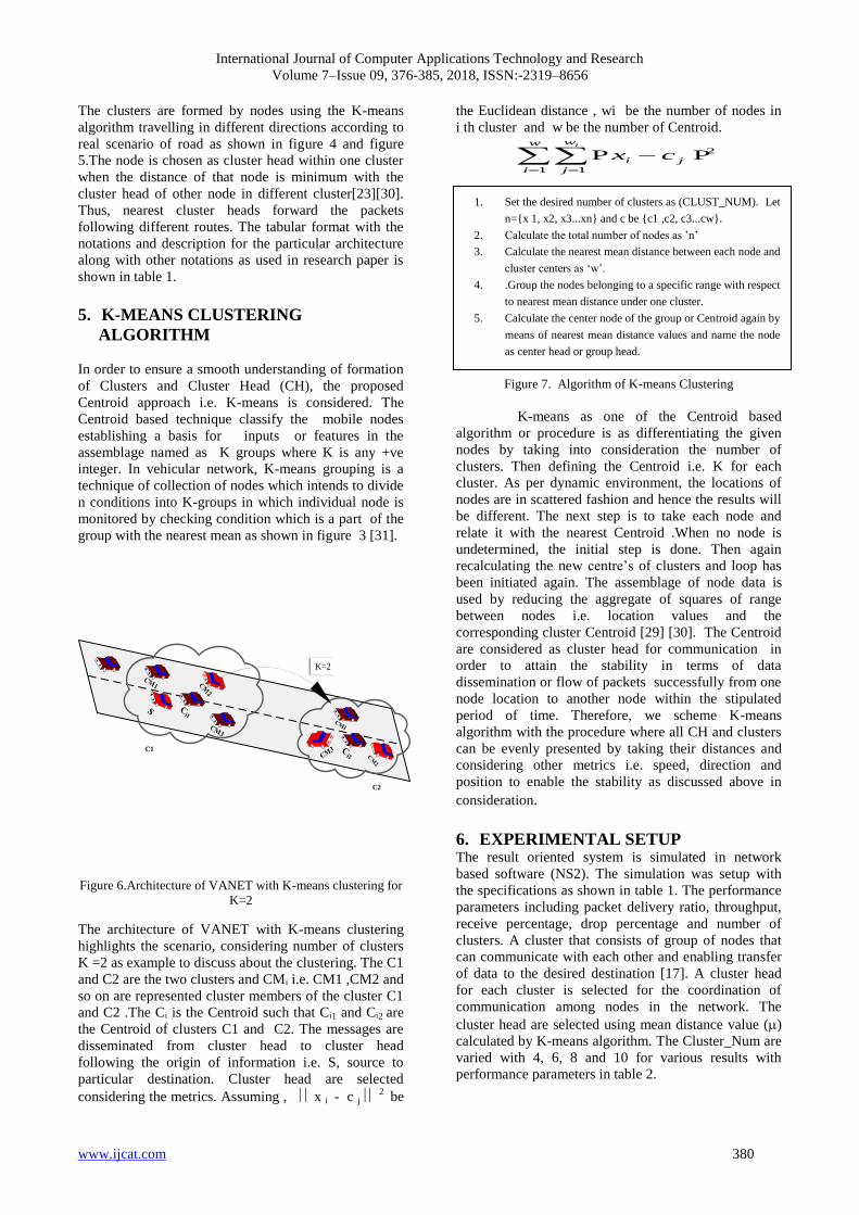
The clusters are formed by nodes using the K-means

algorithm travelling in different directions according to

real scenario of road as shown in figure 4 and figure

5.The node is chosen as cluster head within one cluster

when the distance of that node is minimum with the

cluster head of other node in different cluster[23][30].

Thus, nearest cluster heads forward the packets

following different routes. The tabular format with the

notations and description for the particular architecture

along with other notations as used in research paper is

shown in table 1.

5. K-MEANS CLUSTERING

ALGORITHM

In order to ensure a smooth understanding of formation

of Clusters and Cluster Head (CH), the proposed

Centroid approach i.e. K-means is considered. The

Centroid based technique classify the mobile nodes

establishing a basis for inputs or features in the

assemblage named as K groups where K is any +ve

integer. In vehicular network, K-means grouping is a

technique of collection of nodes which intends to divide

n conditions into K-groups in which individual node is

monitored by checking condition which is a part of the

group with the nearest mean as shown in figure 3 [31].

K=2

C1

C2

Figure 6.Architecture of VANET with K-means clustering for

K=2

The architecture of VANET with K-means clustering

highlights the scenario, considering number of clusters

K =2 as example to discuss about the clustering. The C1

and C2 are the two clusters and CMᵢ i.e. CM1 ,CM2 and

so on are represented cluster members of the cluster C1

and C2 .The Cᵢ is the Centroid such that Cᵢ1 and Cᵢ2 are

the Centroid of clusters C1 and C2. The messages are

disseminated from cluster head to cluster head

following the origin of information i.e. S, source to

particular destination. Cluster head are selected

considering the metrics. Assuming , x i - c j 2

be

the Euclidean distance , wi be the number of nodes in

i th cluster and w be the number of Centroid.

2

1 1

iww

i j

i j

x c

P P

Figure 7. Algorithm of K-means Clustering

K-means as one of the Centroid based

algorithm or procedure is as differentiating the given

nodes by taking into consideration the number of

clusters. Then defining the Centroid i.e. K for each

cluster. As per dynamic environment, the locations of

nodes are in scattered fashion and hence the results will

be different. The next step is to take each node and

relate it with the nearest Centroid .When no node is

undetermined, the initial step is done. Then again

recalculating the new centre’s of clusters and loop has

been initiated again. The assemblage of node data is

used by reducing the aggregate of squares of range

between nodes i.e. location values and the

corresponding cluster Centroid [29] [30]. The Centroid

are considered as cluster head for communication in

order to attain the stability in terms of data

dissemination or flow of packets successfully from one

node location to another node within the stipulated

period of time. Therefore, we scheme K-means

algorithm with the procedure where all CH and clusters

can be evenly presented by taking their distances and

considering other metrics i.e. speed, direction and

position to enable the stability as discussed above in

consideration.

6. EXPERIMENTAL SETUP The result oriented system is simulated in network

based software (NS2). The simulation was setup with

the specifications as shown in table 1. The performance

parameters including packet delivery ratio, throughput,

receive percentage, drop percentage and number of

clusters. A cluster that consists of group of nodes that

can communicate with each other and enabling transfer

of data to the desired destination [17]. A cluster head

for each cluster is selected for the coordination of

communication among nodes in the network. The

cluster head are selected using mean distance value ()

calculated by K-means algorithm. The Cluster_Num are

varied with 4, 6, 8 and 10 for various results with

performance parameters in table 2.

1. Set the desired number of clusters as (CLUST_NUM). Let

n={x 1, x2, x3...xn} and c be {c1 ,c2, c3...cw}.

2. Calculate the total number of nodes as ’n’

3. Calculate the nearest mean distance between each node and

cluster centers as ‘w’.

4. .Group the nodes belonging to a specific range with respect

to nearest mean distance under one cluster.

5. Calculate the center node of the group or Centroid again by

means of nearest mean distance values and name the node

as center head or group head.



www.ijcat.com 381

Table 1.Showing the Setup with Specifications

Attributes Type

Channel

Channel/WirelessChannel

Network interface

Phy/WirelessPhy

Radio propogation

Propogation/TwoRayGround

Interface queue

Queue/DropTail/PriQueue

MAC

Mac/802_11

Antenna

Antenna/OmniAntenna

Link layer

LL

Max packet in ifq

100

Routing protocol

AODV

X dimension of topography

3500m

Y dimension of topography

3500m

Simulation time

60s

7. RESULT ANALYSIS A comprehensive simulations study was regulated to

evaluate the performance of the clusters. In our

simulation, we consider the road traffic and the network

parameters. We simulated a real scenario of road with

particular area coverage includes intersection of roads,

turns, curves and vehicles as shown in figure 4. In

simulation, we investigate 100 vehicles on real world.

The more stable configuration is calculated using the

various parameters quality parameters with their

expected formulas for evaluation of results. The

different parameters includes the packet delivery ratio,

throughput, receive percentage and the drop percentage.

The Cluster_Num are simulated with cluster_ Num 4, 6,

8 and 10. The different colors depicts the clusters in

NS2 with the mobility based file along with the cluster

heads numbered as CH (1), CH (2), CH (3) ….so on are

shown in figure 8, 9, 10 and 11 according to Cluster

_Num 4, 6, 8 and10. The channel to channel

communication and channel to destination

communication in order to deliver the packets following

the different routes. The routing protocol used is AODV

and the topology dimension used is a 3500-3500 meter

with simulation time for each of cluster configuration is

50 s. The mobility file generated with the open street

map and SUMO and exported in NS2 for simulation is

used in the simulation containing the positions of the

nodes.

Table 2.Showing the formulas for packet delivery ratio,

throughput, receive percentage and drop percentage

Parameters Formulae

packet delivery ratio (pdr)

throughput (tp) where t

is

transmis

sion

time

receive percentage (rp)

drop percentage (D)

When the density was zero, the flow was zero, the flow

as observed to be zero against s, r, D. When the flow of

packets gradually increases the density against each

parameter also start increasing. When more and more

packets get added to flow, it reaches saturation point

and gradual drop in density is observe d in each case.

The numbers of clusters are varied & performance is

evaluated based on the parameters as shown in table 3.



www.ijcat.com 382

The density plots are formed in R studio that

includes s, r, f and D for each of the cluster

configuration. The figure 12, figure 13, figure 14 and

figure 15 show the plots for cluster configuration 4, 6, 8

and 10 respectively.

Figure 8. Showing simulation for Cluster_Num 4



Figure 11: Showing simulation for Cluster_Num 10

When the number of mobile nodes were set to 4. The

total number of packets send were 1827 and the total in

density is observed in each case packets received were

found to be 1728. The packet delivery ratio was

105.729 and while the throughput was observed to

276.48 as shown in table 3 and can clearly be observed

in the density plot as shown in Figure12.



www.ijcat.com 383

Table 3: Showing parameters used in comparison as total packets sent, receive, forward, packet delivery ratio, throughput, receive

percentage and drop percentage




found to be 1789. The packet delivery ratio was 10.788

and while the throughput was observed to 286.24 as

shown in table (3) and can clearly be observed in the

density plot as shown in Figure13

Figure 12. Showing density plot for total packets sent (s),

total packets receive(r), total packets forward (f) and total

packets dropped (D) for cluster 4




found to be 2978. The packet delivery ratio was 2295

and while the throughput was observed to 476.48 as

shown in table (3) and can clearly be observed in the

density plot as shown in figure14.







found to be 3203. The packet delivery ratio was

110.240 and while the throughput was observed to

512.48 as shown in table (3) and can clearly be

observed in the density plot as shown in Figure15

Cluster_Num

sent (s)

receive (r)

forward (f)

packet delivery

ratio

(pdr)

throughput

(tp)

receive%

(rp)

drop %

(D)

4 1827 1728 4383 105.729 276.48 94.581 5.419

6 1982 1789 6129 110.788 286.24 90.262 9.737

8 3168 2978 2295 106.380 476.48 94.002 5.997

10 3531 3203 3919 110.240 512.48 90.71 9.289



www.ijcat.com 384







8. CONCLUSION Vehicular Ad-hoc network is an encouraging

technology for facilitating the communication among

the nodes in real environment with Roadside Units

(RSU) that leads to complexity in mobility patterns.

With the movement of nodes, the topology of the

network goes on changing. The dynamic nature of the

nodes in network promotes a lot of technical issues

including the stability of the network in terms of stable

configuration in clusters using real scenario of road

SUMO, open street map and NS2 with K-means

clustering. The simulation shows that the maximum

packet density was observed to <=1.5 in case the

number was set to 4. The density was observed to <=2.0

in case the number of clusters were set to 6,8 and 10 as

illustrated in Figure 12, Figure 13, Figure 14 and Figure

15 respectively. Different performance parameters

which include throughput receive percentage, packet

delivery ratio and drop percentage for evaluating the

performance. This clearly depicts that the flow of

packets optimized with increase in the number of

clusters.

9. REFERENCES [1] EE. C. Eze, S. Zhang and E. Liu, "Vehicular ad hoc

networks (VANETs): Current state, challenges, potentials and

way forward," 2014 20th International Conference on

Automation and Computing, Cranfield, 2014

[2] C. Jeremiah and A. J. Nneka, "Issues and possibilities in

Vehicular Ad-hoc Networks (VANETs)," 2015 International

Conference on Computing, Control, Networking, Electronics

and Embedded Systems Engineering (ICCNEEE), Khartoum,

2015

[3] B. Ayyappan and P. M. Kumar, "Vehicular Ad Hoc

Networks (VANETS): Architectures, methodologies and

design issues," 2016 Second International Conference on

Science Technology Engineering and Management

(ICONSTEM), Chennai, 2016

[4] S. M. AlMheiri and H. S. AlQamzi, "MANETs and

VANETs clustering algorithms: A survey," 2015 IEEE 8th

GCC Conference & Exhibition, Muscat, 2015

[5] Sabih ur Rehman, Lihong Zheng,”Vehicular Adhoc

network & their challenges”, IEEE Vehicular Networking

Conference (VNC), Spain,2014

[6] Mowaesh Zaver and zang li , “VANETS Routing

Protocols and Mobility Models: A Survey” ,2016 Second

International Conference on Science Technology Engineering

and Management (ICONSTEM), vol. 197,2011

[7] Kevin C. Lee and Weijh Lish “Survey of Routing

Protocols in Vehicular Ad Hoc Networks, in IEEE Vehicular

Technology Magazine vol. 21,March 2011

[8] Leize ,IEEE Journal of Information Science and

Engineering “Routing Protocols in Vehicular Ad Hoc

Networks: A Survey and Future Perspectives” vol .26, 913-

932 (2012)

[9] Qi-wu Wu, Wen and Qingzi Liu, "Comparative study of

VANET routing protocols," International Conference on

Cyberspace Technology (CCT 2014), Beijing, 2014.

[10] M. Hassan, H. Vu, and T. Sakurai, “Performance

Analysis of the IEEE 802.11 MAC Protocol for DSRC Safety

Applications,” IEEE Trans. Vehicular Technology, vol. 60,

no. 8, pp. 3882-3896, Oct. 2011.

[11] Y. Gongjun and S. Olariu, “A probabilistic analysis of

link duration in vehicular ad hoc networks,” IEEE Trans.

Intell. Transp. Syst., vol. 12, no. 4, pp. 1227–12

[12]R. Santos, RM Edwards, NL Seed, “ Inter vehicular data

exchange between fast moving road traffic using ad-hoc

cluster based location algorithm and 802.11b direct sequence

spread spectrum radio” , (Post-Graduate Networking

Conference, 2003)



www.ijcat.com 385

[13] F. Yu and S. Biswas, “Self-configuring TDMA protocols

for enhancing vehicle safety with DSRC based vehicle-to-

vehiclecommunications,” IEEE J. Sel. Areas Communication.,

vol. 25, no. 8, pp. 1526–1537, Oct. 2007.

[14] Q. Xu, T. Mak, J. Ko, and R. Sengupta, “Vehicle-to-

vehicle safety mes-saging in DSRC,” in Proc. ACM VANET,

Oct. 2004.

[15] J. Yin, T. ElBatt, G. Yeung, B. Ryu, S. Habermas, H.

Krishnan and T. Talty, Performance Evaluation of Safety

Applications over DSRC Vehicular Ad Hoc Networks, 1st

ACM Workshop on Vehicular Ad Hoc Networks (VANET),

Oct. 2004.

[16] S. Vodopivec, J. Bešter and A. Kos, "A survey on

clustering algorithms for vehicular ad-hoc networks," 2012

35th International Conference on Telecommunications and

Signal Processing (TSP), Prague, 2012.

[17] M. Sood and S. Kanwar, "Clustering in MANET and

VANET: A survey," 2014 International Conference on

Circuits, Systems, Communication and Information

Technology Applications (CSCITA), Mumbai, 2014.

[18] Rong Chai, Bin Yang, Lifan Li, Xiao Sun and Qianbin

Chen, "Clustering-based data transmission algorithms for

VANET," 2013 International Conference on Wireless

Communications and Signal Processing, Hangzhou, 2013.

[19] S. Xu, B. Shen and S. Lee, "A study on clustering

algorithm of VANET environment," 2012 3rd IEEE

International Conference on Network Infrastructure and

Digital Content, Beijing, 2012

[20] S. M. AlMheiri and H. S. AlQamzi, "MANETs and

VANETs clustering algorithms: A survey," 2015 IEEE 8th

GCC Conference & Exhibition, Muscat, 2015.

[21] S. Banerjee and S. Khuller, “A Clustering Scheme for

Hierarchical Control in Multi-hop Wireless Networks,” in

Proceedings of IEEE INFOCOM, April 2001.

[22] T. Taleb, E. Sakhaee, A. Jamalipour, and K.Hashimoto,

“A Stable Routing Protocol to Support ITS Services in

VANET Networks”, IEEE Trans. on Vehicular Technology,

vol. 56, no. 6, Nov. 2007.

[23] S. Almalag and C. Weigle, “Using Traffic Flow for

Cluster Formation in Vehicular Ad-hoc Networks”, IEEE

Trans. Veh. Technol., vol. 77, no. 4, pp. 2440–2450, oct.

2011.

[24] P.Basu,”A Mobility Based metric for clustering in

mobile Ad-hoc Networks,” International Conference on

Distributed Systems workhop,413-418,2011

[25] Zhenxia Zhang ,Azzedine Boukerche and Richard

W.Pazzi,”A novel Multihop Clustering Scheme for vehicular

Ad-hoc networks”, In : Proceedings of the 9th ACM

international symposium on mobility management and

wireless access,19-26,2011.

[26] Y.Rawashdeh and M.Mahmud, “A Novel Algorithm to

form Stable Clusters in Vehicular ad hoc Networks on

highways”, Journal on wireless communications and

networking , jan 2012, springer.

[27] M. Khabazian, S. Aïssa, and M. Mehmet-Ali,

“Performance Modelling of Safety Messages Broadcast in

Vehicular Ad Hoc Networks”, IEEE Trans. on Intelligent

Transportation Systems, vol. 14, no. 1, Mar. 2013.

[28] K. Hafeez, L. Zhao and Z. Niu, “Distributed

Multichannel and Mobility-Aware Cluster-Based MAC

Protocol for Vehicular Ad Hoc Networks”,IEEE Trans. On

Vehicular Technology, vol. 62, no. 8, oct 2013.

[29]Qingwei Zhang, Mohammed Almulla, Yonglin Ren, and

Azzedine Boukerche, “An Efficient Certificate Revocation

Validation Scheme with k-Means Clustering for Vehicular Ad

hoc Networks”, IEEE Symposium on Computers and

Communications (ISCC), 862-867, 2012.

[30] D. Asir Antony Gnana Singh, A. Escalin Fernando, E.

Jebamalar Leavline , “ Performance Analysis on Clustering

Approaches for Gene Expression Data “, International Journal

of Advanced Research in Computer and Communication

Engineering Vol. 5, Issue 2, February2016

Documents

O ptimum L ocation of DG U nits C onsidering O peration C ... · losses, distributed generation units have been spread out in the power distribution systems. In the literature review,