On the Time-optimal Trajectory Planning and Control of Robotic

Manipulators Along Predefined Paths†

Pedro Reynoso-Mora1, Wenjie Chen1, and Masayoshi Tomizuka1

Abstract— In this paper we study the problem of time-optimal trajectory planning and control of robotic manipu-lators along predefined paths. An algorithm that generatesdynamically feasible time-optimal trajectories and controls ispresented, which considers the complete dynamic model withboth Coulomb and viscous friction. Even though the effectsof viscous friction for fast motions become more significantthan Coulomb friction, in previous formulations viscous frictionwas ignored. We propose a formulation that naturally leadsto a convex relaxation which solves exactly the original non-convex formulation. In order to numerically solve the proposed

formulation, a discretization scheme is also developed. Throughsimulation and experimental studies on the resulting trackingerrors, applied torques, and accelerometer readings for a 6-axis manipulator, we emphasize the significance of penalizing ameasure of total jerk. The importance of imposing accelerationconstraints at the initial and final transitions of the trajectoryis also studied.

I. INTRODUCTION

Time-optimality in robotic manipulators is crucial for

maximizing robot productivity. In many industrial applica-

tions of robotic arms, such as palletizing and pick-and-

place, an operator specifies a collision-free path that the

robot must follow in order to accomplish a particular task.

This path specification is usually done through a so-called

teach-pendant or through a path planning algorithm [1].

Once the path has been specified, it is important to find out

how to move the robot along that path in the shortest time

dynamically feasible; first successful approaches to tackle

this problem date back to the 1980s [2], [3], [4]. In the

approaches [2], [3], search algorithms were proposed that

find switching points in the so-called velocity limit curve.

At these switching points, instant changes from maximum

acceleration to maximum deceleration and vice versa must

occur. In [4], additional properties of the velocity limit

curve were pointed out, which allow for simplification in

the computation of the switching points.

Over the past decades, a prominent approach to numerical

optimal control has emerged [5], in which the original

optimal control problem is transcribed directly to a non-

linear optimization problem. In the specific context of time-

optimal trajectories and controls for robotic manipulators

along predefined paths, a modern formulation that uses

tools from convex optimization was proposed in [6]. Even

†The first author acknowledges UC MEXUS-CONACYT for providinghim with a fellowship to support his PhD studies. Also, the financial andtechnical supports from FANUC Corporation are acknowledged.

1Department of Mechanical Engineering, University of Californiaat Berkeley, 94720 CA, USA, {preynoso, wjchen,tomizuka}@me.berkeley.edu

though the effects of viscous friction become noticeably

more significant than Coulomb friction, none of the existing

formulations take into account the complete dynamic model.

In this paper, we propose a formulation that incorporates

the complete dynamic model, which results in a non-convex

optimal control problem. It is then shown how to relax the

referred non-convex formulation so as to obtain a convex

optimal control problem. Because of the way in which both,

the non-convex and the convex formulations are constructed,

it turns out the convex relaxation solves exactly the original

non-convex problem.

Aided by simulations and experimental studies of the

tracking errors, applied torques, and accelerometer readings

on a 6-axis manipulator, we point out the importance of:

(i) penalizing a measure of total jerk, and (ii) imposing

acceleration constraints at the initial and final transitions of

the trajectory. Likewise, a discretization scheme is presented

that allows a straightforward incorporation of these acceler-

ation constraints. Thus, optimal trajectories and controls that

are more realistic than the purely time-optimal solutions are

generated, at the cost of modest increase in the traversal time.

The optimal trajectories and controls are termed dynamically

feasible since the complete dynamic model is incorporated

into the formulation. It is thus verified that the solutions

produced by the algorithm are indeed dynamically feasible

with respect to the complete dynamic model.

In Section II the problem formulation as a mathematical

optimization is presented. Then in Section III a discretiza-

tion scheme is presented that allows to obtain a numerical

solution. In Section IV an application to a 6-axis industrial

manipulator is presented; from simulations on a realistic

simulator, it is argued that pure time-optimal solutions need

to be slightly modified before being implemented on the real

robot. Then, in Section V, specific details for incorporating

acceleration constraints and for penalizing a measure of total

jerk are presented; experimental results are also presented

to report on the benefits of the proposed methodology.

Conclusions are presented in Section VI.

II. PROBLEM FORMULATION

In order to generate trajectories and open-loop controls

that are dynamically feasible, the dynamic model should

take into account the most significant effects present in the

physical system. For an n−DOF manipulator, the equations

of motion take the following standard form [7]:

M(q)q +C(q, q)q+ g(q) +Dvq+ FC sgn(q) = τ , (1)

2013 American Control Conference (ACC)Washington, DC, USA, June 17-19, 2013

978-1-4799-0178-4/$31.00 ©2013 AACC 371

where q, q, q ∈ Rn are the joint-space positions, velocities,

and accelerations, respectively; τ ∈ Rn is the vector of

applied joint torques; M(q),C(q, q) ∈ Rn×n are the inertia

and Coriolis/centrifugal matrices, respectively; g(q) ∈ Rn

represents the vector of gravitational torques; diagonal ma-

trices Dv,FC ∈ Rn×n represent the coefficients of viscous

and Coulomb friction, respectively.

A. Mathematical Formulation

Assume that the geometric path, along which the robot is

required to move, has been determined using for example a

teach-pendant or a path planning algorithm [1]. Then the goal

is to determine how to move along that path in the shortest

time possible. The reference trajectory is denoted by qd ∈R

n, it is then desired to obtain a 4-tuple (qd, qd, qd, τd)that is dynamically feasible with respect to (1) and that

guaranties motion in the shortest time possible. In this

paper, the geometric path is represented by h(s), where sis a monotonically increasing parameter s(t) ∈ [0, 1]. It is

required that h(s) be twice continuously differentiable in s.

It is readily shown from the equality constraint qd = h(s),that qd = h′(s)s and qd = h′′(s)s2 + h′(s)s, where

h′(s) and h′′(s) denote the first and second derivatives

of h(s) with respect to s, respectively. Since the 4-tuple

(qd, qd, qd, τd) must be dynamically feasible with respect

to (1), the expressions for qd and qd are substituted into

(1). Using standard properties of dynamic model (1), and

after some algebraic manipulations, it is obtained:

τd = a1(s)s+ a2(s)s2 + a3(s)s+ a4(s), (2)

where ai(s) ∈ Rn, i = 1, . . . , 4, are defined as:

a1(s) := M (h(s))h′(s)

a2(s) := M (h(s))h′′(s) +C (h(s),h′(s))h′(s)

a3(s) := Dvh′(s)

a4(s) := FC sgn (h′(s)) + g (h(s)) .

Note that ai(s), i = 1, . . . , 4, are entirely known since h(s),h′(s), and h′′(s) are known. The unknowns in parametriza-

tion (2) are s, s2, s, and τd. Consider therefore defining

a(s) := s, b(s) := s2, c(s) := s, and τd(s), which are to be

determined as functions of s. Since a one-to-one relationship

between s and t will be enforced (i.e., s > 0), finding

the unknowns as functions of s implies that they can be

unambiguously recovered as functions of t.

In this manner, τd(s) has a simple affine parametrization

in a(s), b(s), and c(s), namely, τd(s) = a1(s)a(s) +a2(s)b(s)+a3(s)c(s)+a4(s). Likewise, with the definitions

of a(s), b(s), and c(s), two additional constraints must be

incorporated: (i) b(s) = b′(s)s = 2ss ⇔ b′(s) = 2a(s)if s > 0, (ii) c(s) =

√

b(s). On the other hand, the total

traversal time is denoted by tf and can be rewritten in a

different manner, using the fact that s > 0:

tf =

∫ tf

0

dt =

∫ 1

0

(

ds

dt

)−1

ds =

∫ 1

0

1

c(s)ds. (3)

It is important to consider the case when the initial and final

pseudo-speeds are zero, i.e., s0 = sf = 0. In that case, it is

clear that the objective functional (3) is unbounded above.

In order to overcome this limitation, the integral in (3) is

defined instead in the interval [0α, 1α], where 0α = 0+ and

1α = 1− will be formally defined in Section III.

Consider therefore the following optimization problem:

minimizea(s),b(s),c(s),τd(s)

∫ 1α

0α

1

c(s)ds

subject to b(0) = s20, b(1) = s2f

c(0) = s0, c(1) = sf

τd(s) = a1(s)a(s) + a2(s)b(s)

+ a3(s)c(s) + a4(s)

τ ≤ τd(s) ≤ τ

∀s ∈ [0, 1]

b′(s) = 2a(s), c(s) =√

b(s)

b(s), c(s) > 0 (4)

∀s ∈ [0α, 1α]

where τ , τ ∈ Rn represent the lower and upper bounds on

the torques, and s0, sf represent the initial and final pseudo-

speeds along the path, respectively.

It can be argued that formulation (4) is a non-convex

optimal control problem [5], [6], [8]. The non-convexity of

(4) is due to the non-linear equality constraint c(s) =√

b(s)∀s ∈ [0, 1], which shows up because of viscous friction.

For fast motions, viscous friction has a significant effect

in mechanical systems. Therefore instead of ignoring this

term, a convex relaxation that solves exactly the non-convex

formulation (4) is proposed.

B. Convex Relaxation

Since b(s), c(s) > 0 for all s ∈ [0α, 1α], the following

chain of equivalences is true:

√

b(s) = c(s) ⇔1

√

b(s)=

1

c(s)

⇔1

√

b(s)≤

1

c(s),

1

c(s)≤

1√

b(s)

⇔ c(s)2 − b(s) ≤ 0, − c(s)2 + b(s) ≤ 0,

where the inequality constraint c(s)2 − b(s) ≤ 0 is convex

since f(b, c) = c2 − b is a convex function of b, c [8].

On the other hand, −c(s)2 + b(s) ≤ 0 is a concave

inequality constraint. Having concave inequality constraints

in an optimization problem implies that the problem is non-

convex. It is then proposed to drop the concave constraint,

and replace the equality constraint c(s) =√

b(s) in (4) with

the convex inequality constraint 1/√

b(s) ≤ 1/c(s).Because the functional in problem (4) is minimized and

since c(s) > 0, at optimum the inequality 1/√

b(s) ≤ 1/c(s)must be active, i.e., 1/

√

b⋆(s) = 1/c⋆(s) ∀s ∈ [0α, 1α]. This

entails that for all s ∈ [0, 1] the solution a⋆(s), b⋆(s), c⋆(s),τ⋆d (s) to the convex relaxation solves exactly the non-convex

372

problem (4). In order to obtain a convenient formulation of

the convex relaxation, note that ∀s ∈ [0α, 1α] [9]:

1√

b(s)≤

1

c(s)⇔ c(s)2 ≤ b(s) · 1

⇔

∥

∥

∥

∥

[

2c(s)b(s)− 1

]∥

∥

∥

∥

2

≤ b(s) + 1.

Likewise, in order to have a linear objective functional,

assume ∃d(s) > 0 satisfying d(s) ≥ 1/c(s) ∀s ∈ [0α, 1α],then note that:

d(s) ≥1

c(s)⇔ 1 ≤ c(s)d(s)

⇔

∥

∥

∥

∥

[

2c(s)− d(s)

]∥

∥

∥

∥

2

≤ c(s) + d(s).

Therefore, the relaxed problem results in:

minimizea(s),b(s),c(s),τd(s),d(s)

∫ 1α

0α

d(s) ds

subject to b(0) = s20, b(1) = s2f

c(0) = s0, c(1) = sf

τd(s) = a1(s)a(s) + a2(s)b(s)

+ a3(s)c(s) + a4(s)

τ ≤ τd(s) ≤ τ

∀s ∈ [0, 1]

b′(s) = 2a(s)∥

∥

∥

∥

[

2c(s)b(s)− 1

]∥

∥

∥

∥

2

≤ b(s) + 1

∥

∥

∥

∥

[

2c(s)− d(s)

]∥

∥

∥

∥

2

≤ c(s) + d(s)

b(s), c(s) > 0 (5)

∀s ∈ [0α, 1α],

which is a convex optimization problem.

III. PROBLEM DISCRETIZATION

In order to obtain a numerical solution to problem (5),

a discretization scheme should be developed. As discussed

later in Section V, it is important to impose acceleration

constraints, so that smooth acceleration transitions from/to

zero are guaranteed at the initial/final points of the trajectory.

Unlike the approach in [6], where a mid grid had to be de-

fined since a(s) was assumed piecewise constant, we follow

the approach to solve optimal control problems presented in

[10]. This approach, known as cubic collocation at Lobatto

points, will allow us to incorporate the required acceleration

constraints in a straightforward manner.

A. Cubic Collocation at Lobatto Points

First, a grid is created by discretizing the path parameter sinto N points, s1 = 0 < s2 < · · · < sN = 1. Then, it is as-

sumed that b(s) and a(s) are piecewise cubic and piecewise

linear, respectively. Finally, the optimization variables are de-

fined in the following manner: a1 = a(s1), . . . , aN = a(sN ),b1 = b(s1), . . . , bN = b(sN ), c1 = c(s1), . . . , cN = c(sN ),

d1 = d(s1), . . . , dN = d(sN ), τ1 = τd(s1), . . . , τ

N =τd(sN ), which represent the functions a(s), b(s), c(s), d(s),and τd(s) evaluated at the grid points s1 < s2 < · · · < sN .

The pseudo-acceleration a(s) in (5) is chosen as piecewise

linear, i.e.,

a(s) = aj+(aj+1−aj)

(

s− sjsj+1 − sj

)

, s ∈ [sj , sj+1] (6)

j = 1, 2, . . . , N − 1, from which it is noticed that indeed

a(sj) = aj and a(sj+1) = aj+1. The squared pseudo-speed

b(s) is chosen as piecewise cubic, i.e.,

b(s) =

3∑

k=0

βj,k

(

s− sjsj+1 − sj

)k

, s ∈ [sj , sj+1] (7)

j = 1, 2, . . . , N − 1, where the polynomial coefficients

βj,0, βj,1, βj,2, and βj,3 need to be determined explicitly.

The above representation for b(s) must satisfy b(sj) =bj , b(sj+1) = bj+1, b′(sj) = 2a(sj), and b′(sj+1) =2a(sj+1), which gives 4 equations for the four unknowns

βj,0, βj,1, βj,2, and βj,3. After solving, it is obtained:

βj,0 = bj, βj,1 = 2∆sjaj

βj,2 = 3(bj+1 − bj)− 2∆sj(aj+1 + 2aj)

βj,3 = 2∆sj(aj+1 + aj)− 2(bj+1 − bj),

where ∆sj := sj+1 − sj , j = 1, 2, . . . , N − 1.

The approximating functions of a(s) and b(s) in (6)-

(7) must satisfy b′(s) = 2a(s) at the grid points sj , j =1, . . . , N , and at the middle points sj := (sj + sj+1)/2,

j = 1, . . . , N − 1. The coefficients βj,0, βj,1, βj,2, and βj,3

given above already guarantee fulfillment of the constraints

at grid points sj . Therefore, the only constraints that need

to be incorporated result from requiring b′(sj) = 2a(sj),j = 1, . . . , N − 1. After standard algebraic simplifications,

it is shown that this is equivalent to:

bj+1 − bj = ∆sj(aj+1 + aj), j = 1, . . . , N − 1. (8)

Note that enforcing these constraints implies that the coeffi-

cients βj,3 above are zero, which means that actually b(s) is

piecewise quadratic. Since c(s)2 = b(s), it is then reasonable

to assume c(s) is piecewise linear.

Define 0α := (1 − α)s1 + αs2 and 1α := (1 − α)sN +αsN−1, with α > 0 being a small adjustable parameter. Since

d(s) is assumed piecewise linear, the objective functional is

discretized as follows:∫ 1α

0α

d(s) ds =

∫ s2

0α

d(s) ds

+

N−2∑

k=2

∫ sk+1

sk

d(s) ds+

∫ 1α

sN−1

d(s) ds

≈1

2[(1− α)∆s1(d(0α) + d2)

+

N−2∑

k=2

∆sk(dk + dk+1) (9)

+ (1− α)∆sN−1(dN−1 + d(1α))] ,

373

where d(0α) = (1 − α)d1 + αd2 and d(1α) = αdN−1 +(1−α)dN . The constraints in problem (5) are discretized by

simply being evaluated at the grid points sj , j = 1, . . . , N .

For those constraints that are not defined at s1 = 0 and

sN = 1, they are evaluated at 0α and 1α instead. Therefore,

the following convex optimization problem is obtained:

minimizeak,bk,ck,τk,dk

1

2[(1− α)∆s1(d(0α) + d2)

+

N−2∑

k=2

∆sk(dk + dk+1)

+ (1− α)∆sN−1(dN−1 + d(1α))]

subject to b1 = s20, bN = s2f

c1 = s0, cN = sf

τk = a1(sk)ak + a2(sk)bk

+ a3(sk)ck + a4(sk)

τ ≤ τk ≤ τ

∥

∥

∥

∥

[

2ckbk − 1

]∥

∥

∥

∥

2

≤ bk + 1

for k = 1, . . . , N

bj+1 − bj = ∆sj(aj+1 + aj)

for j = 1, . . . , N − 1

bl > 0, cl > 0∥

∥

∥

∥

[

2cl − dl

]∥

∥

∥

∥

2

≤ cl + dl (10)

for l = 2, . . . , N − 1∥

∥

∥

∥

[

2c(0α)− d(0α)

]∥

∥

∥

∥

2

≤ c(0α) + d(0α)

∥

∥

∥

∥

[

2c(1α)− d(1α)

]∥

∥

∥

∥

2

≤ c(1α) + d(1α)

where c(0α) = (1−α)c1 +αc2 and c(1α) = αcN−1 +(1−α)cN . The discretized problem (10) is a Second Order Cone

Program (SOCP), which is a special class of convex opti-

mization problems [6], [8], [9]. This optimization problem is

readily coded and solved using CVX, which is a MATLABr

software for discipline convex optimization.

Notice that by solving problem (10), the optimal functions

a⋆(s), b⋆(s), c⋆(s), d⋆(s), and τ⋆d (s), evaluated at s1 = 0 <

s2 < · · · < sN = 1, are obtained. The optimal 4-

tuple (q⋆d(t), q

⋆d(t), q

⋆d(t), τ

⋆d (t)) is simply recovered from

q⋆d = h′(s)c⋆(s), q⋆

d = h′′(s)b⋆(s) + h′(s)a⋆(s). Likewise,

the corresponding time t(s) can be recovered from d(s)as follows: initialize t(s1) = 0, then for k = 2, . . . , N ,

compute:

t(sk) = t(sk−1) +1

2∆sk−1(dk−1 + dk). (11)

IV. APPLICATION TO A 6-AXIS MANIPULATOR

The time-optimal 4-tuple (q⋆d(t), q

⋆d(t), q

⋆d(t), τ

⋆d (t)) is

generated for a 6-axis industrial manipulator, namely,

FANUC M-16iB. A non-trivial path with non-constant ori-

entation of the end effector is designed. The Cartesian-space

0.80.9

11.1

1.21.3

−1

−0.5

0

0.5

1

0.5

1

1.5

x (m)

y (m)

z(m

)

(a) Cartesian-space path

0 0.2 0.4 0.6 0.8 1

−1

0

1

2

3

0 0.2 0.4 0.6 0.8 1

−20

0

20

0 0.2 0.4 0.6 0.8 1

−1000

0

1000

s (-)

h(s)

(rad

)h′(s)

h′′(s)

h1 h2 h3 h4 h5 h6

(b) Joint-space path

Fig. 1. Non-trivial path used to test the algorithm

path is shown in Fig. 1(a), where the initial and final points

are marked with ‘*’ and ‘o’, respectively. Both the position

and orientation (Euler angles) are interpolated using cubic

splines to satisfy the differentiability requirement on h(s).

A total of N = 1200 points are used to discretize the

parameter s. The Robotics Toolbox for MATLABr is used

to carry out kinematics and dynamics computations [11]. In

Fig. 1(b), the corresponding joint-space path h(s) together

with h′(s) and h′′(s) are presented.

The initial and final speeds are enforced to be zero,

i.e., s0 = sf = 0. The torque constraints τ are com-

puted as follows: for the jth motor, τ j = (1/4)rjkjimaxj ,

where rj is the gear ratio, kj is the torque-current con-

stant, and imaxj the maximum current. Therefore, τ =

(1782.4 1789.7 1647.2 97.2 108.5 79.1)⊤ Nm, which rep-

resents the maximum torques at the link-side, i.e., after

the reducers. The corresponding maximum torques at the

motor-side, i.e., before the reducers, are u = R−1τ =

(10.21 10.21 8.60 4.30 1.58 1.58)⊤ Nm, where R is a

374

0 0.5 1 1.5 2 2.5 3

−10

−5

0

5

10

0 0.5 1 1.5 2 2.5 3

−2

0

2

τ⋆1 τ⋆2 τ⋆3

τ⋆4 τ⋆5 τ⋆6

R−1τ⋆ d(t)

(Nm

)R

−1τ⋆ d(t)

(Nm

)

t (sec)

(a) Time-optimal torques in motor-side, R−1τ⋆

d(t)

0 0.5 1 1.5 2 2.5 30

0.5

1

0 0.2 0.4 0.6 0.8 10

0.5

0 0.2 0.4 0.6 0.8 1

−5

0

5

c⋆(s)√

b⋆(s)

s (-)

s (-)

s(-

)

t (sec)

s(1

/sec

)s

(1/s

ec2)

(b) Pseudo-speed and pseudo-acceleration

Fig. 2. Numerical time-optimal solutions

0 0.5 1 1.5 2 2.5 3

−1

0

1

2

3

0 0.5 1 1.5 2 2.5 3

−2

0

2

0 0.5 1 1.5 2 2.5 3

−40

−20

0

20

t (sec)

q⋆ d(t)

(rad

)q⋆ d(t)

q⋆ d(t)

q⋆1 q⋆2 q⋆3 q⋆4 q⋆5 q⋆6

Fig. 3. Time-optimal trajectory(

q⋆

d(t), q⋆

d(t), q⋆

d(t)

)

diagonal matrix with the gear ratios.

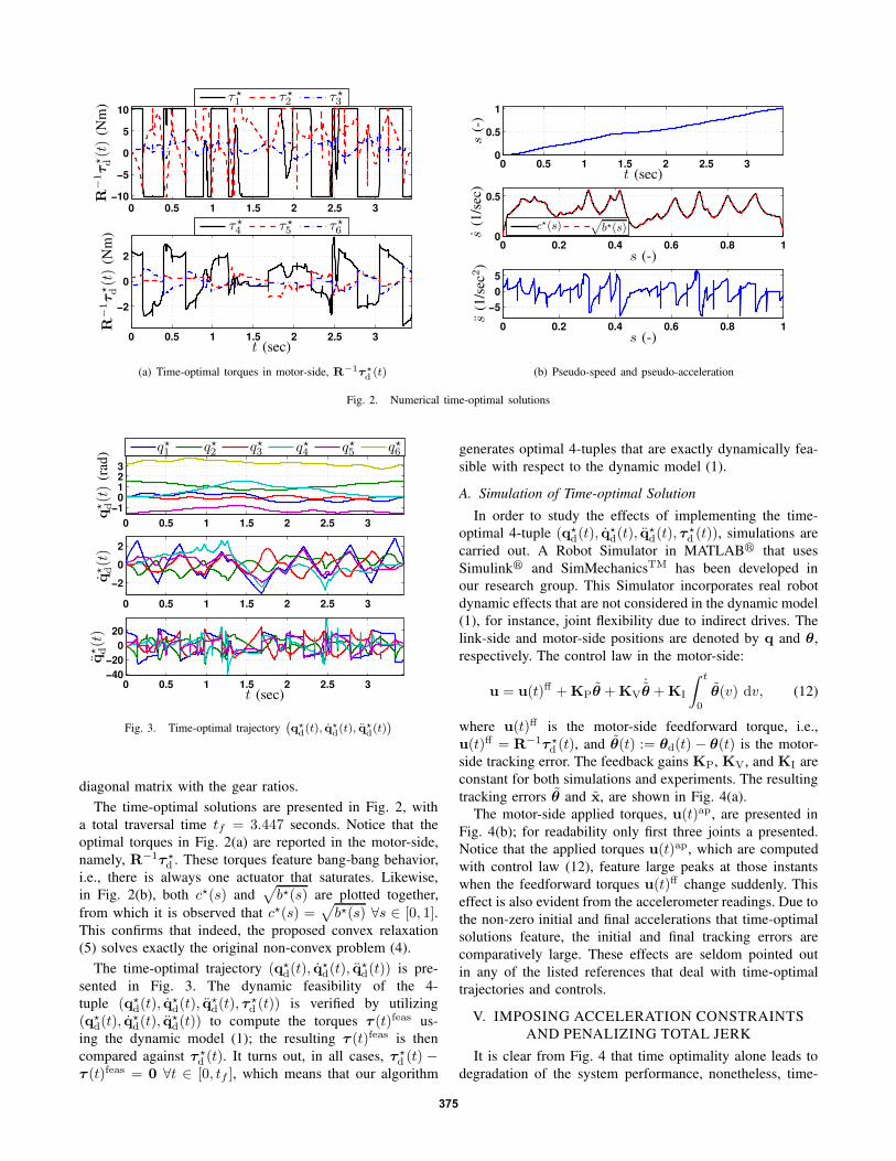
The time-optimal solutions are presented in Fig. 2, with

a total traversal time tf = 3.447 seconds. Notice that the

optimal torques in Fig. 2(a) are reported in the motor-side,

namely, R−1τ⋆d . These torques feature bang-bang behavior,

i.e., there is always one actuator that saturates. Likewise,

in Fig. 2(b), both c⋆(s) and√

b⋆(s) are plotted together,

from which it is observed that c⋆(s) =√

b⋆(s) ∀s ∈ [0, 1].This confirms that indeed, the proposed convex relaxation

(5) solves exactly the original non-convex problem (4).

The time-optimal trajectory (q⋆d(t), q

⋆d(t), q

⋆d(t)) is pre-

sented in Fig. 3. The dynamic feasibility of the 4-

tuple (q⋆d(t), q

⋆d(t), q

⋆d(t), τ

⋆d (t)) is verified by utilizing

(q⋆d(t), q

⋆d(t), q

⋆d(t)) to compute the torques τ (t)feas us-

ing the dynamic model (1); the resulting τ (t)feas is then

compared against τ ⋆d (t). It turns out, in all cases, τ ⋆

d (t) −τ (t)feas = 0 ∀t ∈ [0, tf ], which means that our algorithm

generates optimal 4-tuples that are exactly dynamically fea-

sible with respect to the dynamic model (1).

A. Simulation of Time-optimal Solution

In order to study the effects of implementing the time-

optimal 4-tuple (q⋆d(t), q

⋆d(t), q

⋆d(t), τ

⋆d (t)), simulations are

carried out. A Robot Simulator in MATLABr that uses

Simulinkr and SimMechanicsTM has been developed in

our research group. This Simulator incorporates real robot

dynamic effects that are not considered in the dynamic model

(1), for instance, joint flexibility due to indirect drives. The

link-side and motor-side positions are denoted by q and θ,

respectively. The control law in the motor-side:

u = u(t)ff +KPθ +KV˙θ +KI

∫ t

0

θ(v) dv, (12)

where u(t)ff is the motor-side feedforward torque, i.e.,

u(t)ff = R−1τ⋆d (t), and θ(t) := θd(t) − θ(t) is the motor-

side tracking error. The feedback gains KP, KV, and KI are

constant for both simulations and experiments. The resulting

tracking errors θ and x, are shown in Fig. 4(a).

The motor-side applied torques, u(t)ap, are presented in

Fig. 4(b); for readability only first three joints a presented.

Notice that the applied torques u(t)ap, which are computed

with control law (12), feature large peaks at those instants

when the feedforward torques u(t)ff change suddenly. This

effect is also evident from the accelerometer readings. Due to

the non-zero initial and final accelerations that time-optimal

solutions feature, the initial and final tracking errors are

comparatively large. These effects are seldom pointed out

in any of the listed references that deal with time-optimal

trajectories and controls.

V. IMPOSING ACCELERATION CONSTRAINTS

AND PENALIZING TOTAL JERK

It is clear from Fig. 4 that time optimality alone leads to

degradation of the system performance, nonetheless, time-

375

0 0.5 1 1.5 2 2.5 3

−0.05

0

0.05

0 0.5 1 1.5 2 2.5 3

−0.04

−0.02

0

θ1 θ2 θ3 θ4 θ5 θ6

x y z

θ(t)

(rad

)x(t)

(m)

t (sec)

(a) Motor-side and Cartesian tracking errors

0 0.5 1 1.5 2 2.5 3

−10

0

10

20

0 0.5 1 1.5 2 2.5 3

−40

−20

0

20

40

uap1 uap

2 uap3

x y z

u(t)a

p(N

m)

x(t)

(m/s

ec2)

t (sec)

(b) Applied torques and accelerometer readings

Fig. 4. Simulation results for the time-optimal solution

qi(s)

qMaxi

0 1s ss

Fig. 5. Profile of joint-space acceleration constraints

optimal trajectories and controls are important for increase of

robot productivity. Therefore, it is still desirable to consider

problem (10), and incorporate acceleration constraints that

guarantee smooth acceleration growth (resp. decay) from

zero (resp. to zero) at the the initial (resp. final) point of

the trajectory. Additionally, a term that penalizes a measure

of total jerk will prove to be useful.

A. Acceleration Constraints

Consider imposing joint-space acceleration constraints

with the profile shown in Fig. 5, for each qi(s), i = 1, . . . , n,

where qMaxi represents the maximum acceleration at interme-

diate points. In vector form, −q(s) ≤ qd(s) ≤ q(s), which

is readily discretized as:

−q(sk) ≤ h′′(sk)bk + h′(sk)ak ≤ q(sk) (13)

for k = 1, . . . , N . Inequality constraints (13) are therefore

incorporated to problem (10).

B. Penalizing a Measure of Total Jerk

We are interested in...q , but the forthcoming derivation

follows similar lines for τ (see [6]).

λ

∫ tf

0

‖...q‖1 dt = λ

n∑

i=1

∫ tf

0

|...q i| dt

= λ

n∑

i=1

∫ tf

0

∣

∣

∣

∣

dqidt

∣

∣

∣

∣

dt

= λ

n∑

i=1

∫ 1

0

∣

∣

∣

∣

dqids

∣

∣

∣

∣

ds

≈ λ

n∑

i=1

N−1∑

j=1

|qi(sj+1)− qi(sj)|

∝ λ

n∑

i=1

N−1∑

j=1

|qi(sj+1)− qi(sj)|

qMaxi

. (14)

By introducing the slack variables eij , i = 1, . . . , n, j =1, . . . , N − 1, such that |qi(sj+1)− qi(sj)| ≤ qMax

i eij , (14)

can be replaced with the linear objective function

Jjerk = λn∑

i=1

N−1∑

j=1

eij , (15)

which is incorporated into the objective of problem

(10) to trade off the traversal time. The constraints

|qi(sj+1)− qi(sj)| ≤ qMaxi eij , are expressed compactly by

defining ej := (e1j e2j · · · enj)⊤ ∈ R

n. Therefore,

−ej ∗ qMax ≤ h′′(sj+1)bj+1 + h′(sj+1)aj+1

− h′′(sj)bj − h′(sj)aj ≤ ej ∗ qMax,

for j = 1, . . . , N − 1, where ej ∗ qMax means element-wise

multiplication. These are the final constraints that need to be

incorporated to problem (10).

C. Experimental Results

We generate optimal 4-tuples (q⋆d(t), q

⋆d(t), q

⋆d(t), τ

⋆d (t))

for the 6-axis manipulator FANUC M-16iB. Here we present

the results for λ = 0.02, and for the acceleration con-

straint parameters s = 0.02, s = 0.98, and qMax =(60 60 60 30 30 30)⊤ rad/sec2. Some representative variables

that the algorithm generates are shown in Fig. 6. Notice

that exact zero acceleration is indeed enforced at the be-

ginning/end of the trajectory, with a smooth growth/decay.

Also notice that at the intermediate points sudden changes

376

0 0.5 1 1.5 2 2.5 3 3.5 4

−10

−5

0

5

10

0 0.5 1 1.5 2 2.5 3 3.5 4

−10

0

10

q⋆1 q⋆2 q⋆3 q⋆4

q⋆ d(t)

(rad

/sec

2)

τ⋆1 τ⋆2 τ⋆3R

−1τ⋆ d(t)

(Nm

)

t (sec)

Fig. 6. Representative variables from algorithm results for λ = 0.02

0 0.5 1 1.5 2 2.5 3 3.5 4

−10

−5

0

5

10

0 0.5 1 1.5 2 2.5 3 3.5 4

−20

0

20

uap1 uap

2 uap3 uap

4 uap5 uap

6

x y z

u(t)a

p(N

m)

x(t)

(m/s

ec2)

t (sec)

Fig. 7. Experimental applied torques and accelerometer readings

are eliminated. These benefits come at the cost of a modest

increase in the traversal time, i.e., tf = 4.238 seconds,

which means that this solution is slower than the purely time-

optimal by only 0.791 seconds. Nonetheless, the benefits in

terms of performance become a crucial factor to justify our

development.

Experimental results are presented in Figs. 7 and 8. Note

that the applied torques u(t)ap are close to the feedforward

torques u(t)ff in Fig. 6, and therefore u(t)ap do not exceed

the torque limits. Also, the accelerometer readings of Fig. 7

should be compared against the ones in Fig. 4(b). The corre-

sponding motor-side and Cartesian-space tracking errors are

presented in Fig. 8, all of which are comparatively better than

the ones in Fig. 4(a). Our methodology therefore generates

the fastest solutions that can actually be implemented in the

real system, without degrading its performance.

VI. CONCLUSIONS

An algorithm that generates optimal trajectories and con-

trols was studied. Initially, pure time-optimality was con-

0 0.5 1 1.5 2 2.5 3 3.5 4

−0.01

0

0.01

0 0.5 1 1.5 2 2.5 3 3.5 4

−5

0

5

x 10−3

θ1 θ2 θ3 θ4 θ5 θ6

x y z

θ(t)

(rad

)x(t)

(m)

t (sec)

Fig. 8. Experimental motor-side and Cartesian-space tracking errors

sidered. Then, acceleration constraints and penalization of

a measure of total jerk were incorporated, both of which

proved useful from real experiments on a 6-axis industrial

manipulator. In all cases, the resulting optimal trajectories

and controls are always dynamically feasible with respect

to the complete dynamic model (1), which brings a modest

theoretical and practical extension to existing algorithms.

REFERENCES

[1] S. M. LaValle, Planning Algorithms. Cambridge, U.K.: CambridgeUniversity Press, 2006, available at http://planning.cs.uiuc.edu/.

[2] J. Bobrow, S. Dubowsky, and J. Gibson, “Time-Optimal Controlof Robotic Manipulators Along Specified Paths,” The International

Journal of Robotics Research, vol. 4, no. 3, pp. 3–17, 1985.[3] K. G. Shin and N. D. McKay, “Minimum-time control of robotic

manipulators with geometric path constraints,” IEEE Transactions on

Automatic Control, vol. 30, no. 6, pp. 531–541, 1985.[4] F. Pfeiffer and R. Johanni, “A concept for manipulator trajectory

planning,” Robotics and Automation, IEEE Journal of, vol. 3, no. 2,pp. 115–123, April 1987.

[5] J. T. Betts, Practical methods for optimal control using nonlinear

programming, ser. Advances in Design and Control. Philadelphia,PA: Society for Industrial and Applied Mathematics (SIAM), 2001,vol. 3.

[6] D. Verscheure, B. Demeulenaere, J. Swevers, J. De Schutter, andM. Diehl, “Time-optimal path tracking for robots: a convex optimiza-tion approach,” IEEE Transactions on Automatic Control, 2008.

[7] B. Siciliano, L. Sciavicco, L. Villani, and G. Oriolo, Robotics:

Modelling, Planning and Control, 1st ed., ser. Advanced Textbooksin Control and Signal Processing. Springer-Verlag, 2009.

[8] S. Boyd and L. Vandenberghe, Convex Optimization, 1st ed.Cambridge University Press, 2004, [Online]. Available:http://www.stanford.edu/ boyd/cvxbook/.

[9] L. I, L. Vandenberghe, H. Lebret, and S. Boyd, “Appli-cations of second-order cone programming,” Linear Algebra

and its Applications, pp. 193–228, 1998, [Online]. Available:http://www.stanford.edu/ boyd/papers/socp.html.

[10] O. V. Stryk, “Numerical solution of optimal controlproblems by direct collocation,” 1993. [Online]. Available:http://citeseer.ist.psu.edu/69756.html; http://www-m2.mathematik.tu-muenchen.de/ stryk/paper/1991-dircol.ps.gz

[11] P. Corke, “A robotics toolbox for MATLAB,” IEEE Robotics and

Automation Magazine, vol. 3, no. 1, pp. 24–32, March 1996.

377