O n th e b eh a v io r o f a n eu ra l o scilla to r ... · O n th e b eh a v io r o f a n eu ra l o scilla to r electrica lly co u p led to a b ista b le elem en t Nancy Kopell a

ELSEVIER Physica D 121 (1998) 367-395

On the behavior of a neural oscillator electrically coupled to a bistable element

Nancy Kopell a,, , L.F. Abbot t b, Cristina Soto-Trevifio a a Department of Mathematics, Boston University, Boston, MA 02215, USA

b Volen Center for Complex Systems, Brandeis University, Waltham, MA 02254, USA

Received 11 July 1997; received in revised form 28 January 1998; accepted 4 February 1998 Communicated by C.K.R.T. Jones

Abstract

We study the periodic solutions of a two-cell network consisting of a relaxation oscillator and a bistable element. The aim is to understand how the frequency and wave form of the network depend on the intrinsic properties of the cells and on the strength of the coupling between them. The network equations constitute a fast-slow system; we show that there are four curves of saddle-node points of the fast system whose geometry in parameter space encodes information about the wave form and frequency. These curves give information about the value of the variables at which transitions are made between high and low voltage states for either of the elements, and how those transition points in phase space depend on the coupling strength. Furthermore, we develop a new geometric method to construct the curves of saddle-nodes from families of curves associated with the equations for each of the two cells. The construction allows one to see how changes in either of the elements affects the wave form of the network output. The analysis also shows that the network can produce unintuitive behavior. For example, though electric coupling may keep the network pinned longer at a higher or lower voltage level than the uncoupled oscillator, larger values of the coupling strength may be less effective at this pinning. © 1998 Elsevier Science B.V. All rights reserved.

Keywords: Oscillations; Wave form; Bistable element; Electrical coupling

I. Introduction

Electrical coupling between neurons is often modeled by discrete diffusion. If the cells being coupled are identical, it is clear that synchronous behavior is possible. The effect of the coupling is less clear when the interacting cells are fundamentally different in their uncoupled dynamics. This paper focuses on the interaction of an oscillator and a bistable cell; the oscil lator is of a relaxation type, mimicking the envelope of spikes of a bursting neuron. The study is motivated by a subnetwork in the crustacean stomatogastric ganglion in which the pacemaker is a pair of such electrically coupled cells [ 1,2]. One purpose of this paper is to clarify how the interactions of the dynamics and the

* Corresponding author. Tel.: +1 617 353 5210; fax: +1 617 353 8100; e-mail: [email protected].

0167-2789/98/$19.00 © 1998 Elsevier Science B.V. All rights reserved. PII: S01 67-27 89(98)0003 1- 1

368 N. Kopell et al . /Physica D 121 (1998) 367-395

w increas ing

A

v

Fig. 1. Graphs of v ~ f ( v , w) for different values of w. The graphs are higher for lower values of w, and the shapes are not necessarily the same, though they are all assumed to be qualitatively cubic.

f(v, w ~ h ( v , = o w) = 0

Fig. 2. Eq. ( 1.1 ) has a stable limit cycle with two fast and two slow pieces.

coupling leads to changes in relative timing of the on and off portions of a burst. The clarifications will allow us to make detailed predictions about the range of possible behaviors of such a network.

We shall use simple descriptions of the oscillator and the bistable element, but the analysis can be extended to more complicated systems with the same basic features. The oscillator will be described by a system of the form

cAl dv / dt = f'(v, w), (l . la)

d w / dt = ~h(v, w), e << 1. (1.1b)

In these equations, the v represents the voltage, b"l is the capacitance and the slow variable w is a measure of some recovery process. For each fixed w, the function v ~ 7(v, w) is assumed to have a qualitatively cubic shape, and Of/Ow < 0 (see Fig. I). The nullcline f ( v , w) = 0 is also "cubic," with f > 0 below the cubic and f < 0 above the cubic (see Fig. 2.). (For example, if f ( v , w) -- f ( v ) - w then all the curves of Fig. 1 are vertical translations

N. Kopell et al./Physica D 121 (1998) 367-395

x

x

Fig. 3. The graph o f x ~ g(x) is also qualitatively cubic and has three zeros.

369

of w = .f(v).) The function h is chosen to be positive on the right-hand branch of v ~ f ( v , w) over the range of relevant w, and negative over the left-hand branch. This insures that (1.1) has a stable periodic limit cycle; in the limit ~ ~ 0, the periodic trajectory is as in Fig. 2. An example of a system such as (1.1) is the Morris-Lecar equations [3], often used to model the envelope of a bursting neuron.

The bistable cell is described even more simply: In the absence of coupling, it is given by ~'2 d x / d t = ~(x), where x is the voltage of the cell and ~'(x) is a cubic shaped function with three zeros, the outer two of which correspond to stable critical points for the uncoupled x equation (see Fig. 3). Its recovery processes are omitted, and the equation describes only the fast dynamics of the voltage between two stable states.

The cells are coupled via diffusion of electrical current; this is modeled by discrete diffusion of the voltage variables. Thus, the full equations are

d d ~ l d v / d t = f ' ( v , w ) + - ( x - v ) , d w / d t = ~ h ( v , w ) , ~ 2 d x / d t = g ( x ) + (v - x),

p l - p

where ~ << 1. Here p represents the ratio of the surface area of the oscillator to the total surface area of the two cells, and d is the strength of the electrical synapse.

The above equations can be simplified by letting c] = P~'I, c2 = (1 - P)~2, f = p f , and g = (1 - p)~'. The equations then become

Cl dv/dt = f ( v , w) + d(x - v), dw/dt = ~h(v, w), c2 dx/dt = g(x) + d(v - x). (1.2)

These equations have two fast and one slow variable, and a parameter d. We are interested in finding the periodic solutions of the coupled system (1.2), and in understanding how the coupling and the intrinsic properties of the cells determine the wave forms of the output of the coupled network. We shall construct the periodic solutions by first constructing singular solutions in the limit ~ --+ 0.

Singular solutions to ( 1.2) are constructed as the union of solutions to simpler equations. The "fast equations", whose solutions are the jumps between the slow segments of the trajectory, are

c l d v / d t = f ( v , w ) + d ( x - v ) , c2dx/dt = g ( x ) + d ( v - x ) . (1.3)

In (1.3), w and d both act as parameters. The slow segments are determined by

dw/dt = Eh(v, w), (1.4)

where v = v (w, d) is the v-component of a (w, d) dependent critical point of the fast equations (1.3). The "matching condition" is that each fast solution has as its limit points (as t ~ ±c~) the end points of adjacent slow segments.

There are different kinds of singular solutions for different classes of singularly perturbed equations such as (1.2), depending on the stability of the relevant critical points of the fast system. In our case, the relevant critical points of

370 N. Kopell et al./Physica D 121 (1998) 367-395

( 1.3) turn out to be the stable ones, which will be shown to be bounded by curves (in the w, d plane) of parameters at which (1.3) has a saddle-node point. It will be shown that each fast segment begins at a saddle-node; equivalently, each slow segment ends when the trajectory reaches a saddle-node for ( 1.3). For such singular solutions, it is proved in [4] that for ~ << 1, there are nearby solutions to the full equation (1.2). Thus, we are free to concentrate on the behavior of the singular solutions. We note that the periodic solutions that we construct are asymptotically stable. This is discussed more in Remark 2.4 below.

For two-dimensional relaxation oscillators, as in Fig. 2, it is easy to construct the singular solution from the cubic-shaped nullclines of the fast variable. The singular solution moves along that nullcline and jumps at each of its "knees"; each knee, or local extremum of the nullcline, is a saddle-node for the fast dynamics. In (1.2), the singular periodic solutions again move along a one-dimensional submanifold, which is the "slow manifold" of the system, and jump at points on the slow manifold that are saddle-nodes for the fast dynamics. However, these slow manifolds and their saddle-node boundaries are now no longer as evident from the equations.

In this paper, we give two kinds of results. One set of results (Section 3) concerns the construction of the saddle- node boundaries from the shapes of the v --+ f ( v , w), x ~ - g ( x ) curves and their relative placement. The other set (given in Section 2) shows how one can deduce the wave forms and frequency of the periodic solutions from these saddle-node boundaries. Using the two sets of results, we can see how changing f or g or the coupling strength d can change the periodic solution.

More specifically, Section 2 contains the construction of the periodic solution, once the saddle-node curves are known (e.g. from numerical calculation or the construction of Section 3). Some technical points are only stated there, with details postponed to Section 4. Without further information, this gives the shape of the trajectory in phase space, but not necessarily the time dependence. However, if the nullcline h(v, w) is relatively flat over the slow branches of the trajectory (as in Fig. 2), the saddle-node curves also turn out to give qualitative information about the times spent on each branch. We show that for some classes of functions f , g there is a finite value of d for which the periodic trajectory is held for the longest time on a given branch. Thus, though the electrical coupling can act to pin the network trajectory to its low or high branch for a longer or shorter time than the trajectory of the uncoupled oscillator, larger values of the coupling will not necessarily be more efficient at doing this.

We are also able to deduce conditions on the saddle-node boundary curves for which the behavior is even less intuitive. For example, we see how changes in either of the circuit elements, without changing coupling strength, can drastically change the behavior of the circuit, e.g. acting to functionally couple or uncouple the circuit. We also show that there are conditions under which the bistable element jumps ahead of the oscillator that is "causing" the jump. There are other conditions for which there is an interval in d such that the oscillator is unable to get the bistable to jump with it, while at both higher and lower values of d, the elements do jump together. Another unexpected conclusion is that electrical coupling can act to turn the bistable element permanently to its low or high position. Depending on the properties of h, coupling with the bistable element may also keep the oscillator permanently in its low or high position.

One difficult part of Section 2 is the determination of where each fast portion of a singular trajectory goes when it leaves a saddle-node point of ( 1.3). It is not hard to show, for these equations, that the fast portion must go (as t -+ ~ ) to another critical point. However, for some regions of the d, w plane, there is more than one stable critical point of (1.3). For general equations, the t --~ ~ limit of particular trajectories cannot be deduced simply from the position of the critical points of the fast equation. By contrast, for equations of the form (1.3) we show that, at a non-degenerate saddle-node of the system, the unique unstable manifold must tend to the "nearest" other critical point in the "correct" direction, which is shown to be well-defined. Using this, we are able to provide some rules governing the fast jumps between the slow manifolds.

N. Kopell et al./Physica D 121 (1998) 367-395 371

In Section 3, we show how the shapes of the curves v --~ f ( v , w) and x ~ g(x) , as well as their placement with respect to one another, determine important features of the saddle-node boundary curves in the d, w plane. The techniques also show how the ratio p of the surface area of the oscillator to the total surface area of the two cells affects the position of the curves. To construct the curves of saddle-nodes, we introduce a new geometric method for reading off the qualitative shape of the saddle-node curves from the shapes of v ~ f ( v , w), x ~ g(x) and their placement. Though we are interested in the value of w at which a saddle-node of (1.3) is reached for a fixed d, it turns out to be easier to construct the sets of stable critical points of (1.3) for fixed w and varying d; the curves we seek are the boundaries of these sets. The construction makes strong use of the structure of (1.3), particularly the fact that the coupling currents are equal and opposite. Section 3 states the results connecting the equations to the shapes of the saddle-node curves, and gives the main ideas of the proofs; the technical points are again postponed to Section 4.

Section 4 contains mathematical details postponed from previous sections. Section 4.1 discusses the construction of the saddle-node curves via the implicit function theorm, and makes explicit the conditions for having non- degenerate saddle-nodes. It also contains the proof that, along a slow trajectory, stability for the fast system is lost at a saddle-node, not through a Hopf bifurcation. Section 4.2 shows that for the electrically coupled system, the projection of the full trajectory to the v, w plane is qualitatively like that of the uncoupled system. Section 4.3 proves assertions in Section 2 about the destinations of the fast jumps. Section 4.4 gives the proofs of the assertions in Section 3 connecting the geometry of the equations with the shapes of the trajectories in phase space (and therefore the times in the high and low voltage modes).

The discussion in Section 5 contains two parts. The first concerns a motivating example from the perspective of the theory developed in the paper. The example, from [2], deals with a pair of cells in the crustacean stomatogastric ganglion that are electrically coupled, and that have been modeled in simulations by equations having the form (1.2) plus a slow current added to the bistable element. The simulation in [2] shows how that coupled pair, but not the oscillator alone, is capable of regulating itself so that the proportion of time the cells burst does not change when the frequency is modified (e.g. by current injected into the oscillator). This regulation is known as "constant duty cycle" behavior. The theory of this paper addresses the prior question of how the extra slow current can modulate the times in the active position to compensate for imposed changes in the time spent in the inactive period. We also show, from the geometry, why the equilibrium produced in [2] is a stable one. The second part of Section 5 discusses related work and extensions of the current work.

2. Saddle-node curves and singular solutions

We first give some information (to be proved in Section 5.1 ) about the saddle-node curves. We then show how the singular solutions are constructed once the saddle-node curves are known. Finally, we discuss the kind of information that can be read off from knowledge of the saddle-node curves.

2.1. The four saddle-node curves

There are four curves in d, w space that are of particular interest. These are the projections to d, w space of the boundaries of four two-dimensional surfaces in v, x, d, w space that are the stable critical points of (1.3). (The latter corresponds to the "slow manifold" of (1.2).) The projected curves are bounded at d = 0 by four points that we now describe. Assume that f ( v , w) and g(x) are cubic as in Figs. 1 and 3. Let XL and XH denote the two stable critical points of dx /d t = g(x). (see Fig. 3.) We denote by w = WL and w = WH the two values at which v ~ f ( v , w) has a "knee" (i.e., Of~Or = 0), where f = 0, see Figs. 4(A) and (B). Let VL denote the value of v on the lower


A)

B)

v ~ f(v, WL)

v

v

Fig. 4. The graphs of v ---* f ( v , w) at w = WL, WH. (A) At w = tVL, the local m i n i m u m of f takes the value f = 0. (B) At w = WH, the local m a x i m u m takes the value f = 0.

branch corresponding to this knee for w --//3 L. Similarly, OH is the value of v on the higher branch corresponding to the value w = wn. At d = 0 there are four saddle-nodes. They are:

HH: V=VH, X = X H , W = W H , LL: V = V L , X----XL, W = W E , (2.1) HL: v = o H , X = X L , W = W H , LH: V = V L , X = X H , W = W L .

It will be proved in Section 5.1 that there is a curve of saddle-nodes (in v, x, d, w space) ending at each of the points of (2.1). These curves can be parametrized by d, and are smooth at almost all points. We shall refer to those curves by the name of the point at d = 0: HH, LL, HL or LH. Sometimes, when the meaning is clear, we shall also use HH, etc. to refer to the projection of the curve to the d, w space. For LH and HL, the boundary consists of more than one section parametrized by d. When we say saddle-node, we shall always mean a critical point of (1.3) with one negative and one zero eigenvalue.

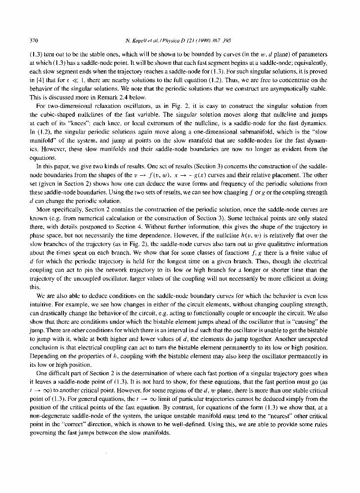
In Section 3, we give conditions on f and g under which the HH curve, projected to the d, w plane, may have any of the shapes in Fig. 5. In each of the cases, the curve begins at d = 0, w = WH, can be written as the graph of w = w(d), and has a vertical asymptote. Depending on the choices of f and g, the curves may have w decreasing as d increases (case A), w increasing as d increases (case B), or w not monotonic in d (cases C and D). The vertical asymptote can be either to the left of w = WH (cases A, D) or to the right (cases B, C). The filled in area denotes the parameter values for which (1.3) has stable critical points. For the LL curve, possible cases are the mirror images of those in Fig. 5, with the initial point at w = WL, d ---- 0. As discussed in Section 3, the pictures in Fig. 5 are not a complete classification; they are intended to illustrate some of the possible behaviors of the curve. As will be seen below, a change of shape of one or more of these curves (by changing f and/or g) changes the singular trajectories. In case D, the singular solution can have peculiar properties, described in Section 2.3.

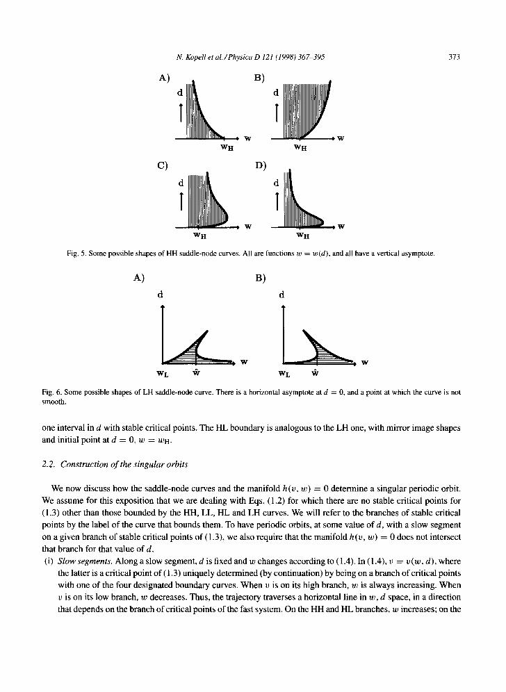
The LH and HL curves are more complicated. Under conditions specified in Section 3, the LH curve begins at d = 0, w = W L and is parametrized smoothly by d for d < dmax < oo. There is another branch of the boundary curve, also parametrized by d for 0 < d < dmax (see Fig. 6(A) and (B)). For some values of w, there is more than

N. Kopell et aL/Physica D 121 (1998) 367-395 373

A) B)

W I W WH WH

c) D)

WH WH W

Fig. 5. Some possible shapes of HH saddle-node curves. All are functions w = w(d), and all have a vertical asymptote.

A) B) d d

w w

WL ~r WL

Fig. 6. Some possible shapes of LH saddle-node curve. There is a horizontal asymptote at d = 0, and a point at which the curve is not smooth.

one interval in d with stable critical points. The HL boundary is analogous to the LH one, with mirror image shapes and initial point at d = 0, w = WH.

2.2. Construction of the singular orbits

We now discuss how the saddle-node curves and the manifold h(v, w) = 0 determine a singular periodic orbit. We assume for this exposition that we are dealing with Eqs. (1.2) for which there are no stable critical points for (1.3) other than those bounded by the HH, LL, HL and LH curves. We will refer to the branches of stable critical points by the label of the curve that bounds them. To have periodic orbits, at some value of d, with a slow segment on a given branch of stable critical points of (1.3), we also require that the manifold h(v, w) = 0 does not intersect that branch for that value of d. (i) Slow segments. Along a slow segment, d is fixed and w changes according to (1.4). In (1.4), v = v(w, d), where

the latter is a critical point of (1.3) uniquely determined (by continuation) by being on a branch of critical points with one of the four designated boundary curves. When v is on its high branch, w is always increasing. When v is on its low branch, w decreases. Thus, the trajectory traverses a horizontal line in w, d space, in a direction that depends on the branch of critical points of the fast system. On the HH and HL branches, w increases; on the


L L s a d d l e - n o d e s H H saddle-nodes

d

stable p o i n t s - -

1 I I I I I I I I I I I I I I I I I I I I I I I I I I I

I " I I , , I ' ,I ,," I t" , , I I I I I I I I I I I . . . . . . . . . . t ' , t " I I I I I I I I I l I I I I I I I I I I I I I I I I I

I I I I I I I I I I I

~ l k l l I I I I I I I I . . . . . . . . ,,,,,,, ~ , ' " I l l l I I I I I I I I I I ii , , I I I , , ,

~ WL

I I I I I I I 1 ~ I I I I I I I I m I l l l l l l l l I I I I I I 1 | I I I I I I I I I I I I I l l I I I I I I I I I I I I I I

I I I I I I I I I I ~ . . . . . L L . . . . stable ~" I < points

WH Wl

Fig. 7. Projection onto d,w space for a periodic trajectory whose slow portions traverse between the LL and HH branches. On HH (resp. LL) the slow portion moves with w increasing (resp. decreasing).

LL and LH branches, w decreases. Unlike the case of a single two-dimensional relaxation oscillator, the slow trajectory does not follow a nullcline or even any of the cubics of Fig. 1. However, it is qualitatively similar, in that the projection of the trajectory to v, w space satisfies dv /dw < 0 along slow segments, as in Fig. 2. The proof of this is given in Section 4.2.

To put together the slow segments and the fast jumps, we start with the case in which the only stable critical points are those bounded by HH and LL. (For many equations, including those whose saddle-node curves are given in Fig. 6, there are no HL or LH stable points for d large enough.) For definiteness, we illustrate one possible set of HH and LL curves in Fig. 7. The region filled in with vertical (resp. horizontal) lines are the values of d, w for which (1.3) has a stable critical point corresponding to both v and x high (resp. low). For a fixed value o l d , the value of w in a slow segment travels along the dark horizontal line segment in Fig. 7, with end points at w = w0 and w = Wl on the saddle-node curves. While w is moving to the right, v = v(w, d) and x = x(w, d) are coordinates of the stable critical point of (1.3) that is a continuation of the point on the saddle-node curve HH; while w is moving to the left, they are coordinates of the critical point that is the continuation of the point on the saddle-node curve LL. If h(v, w) = 0 does not intersect the HH or LL slow manifold (in 4-space) along the slow segment, the trajectory of the slow system must exit at a saddle-node curve. At w = w0 the trajectory jumps; the values of d and w remain fixed, but the values of v and x jump from the coordinates of the LL saddle-node point to those of the HH stable point, and similarly in the other direction. This statement is a special case of the more general rules discussed below (and proved in Section 4.2) concerning the behavior of the fast segments.

(ii) The fast jumps. For some values of d and w, there may be more than one stable critical point to which the fast trajectory might go. Furthermore, it is not clear, without analysis of the fast dynamics (1.3), that the system must jump to another critical point. In this section, we describe the rules that constrain the fast behavior; the proofs are in Section 4.2.

The main result of this section says that, on leaving a slow segment at a saddle-node for (1.3), the fast dynamics takes the trajectory to the "nearest" other critical point in the "correct" direction. More precisely, a non-degenerate saddle-node (~, 2) has a unique unstable manifold, which is the jump trajectory (Fig. 8). The lines v = ~ and x = 2 divide the v, x plane into quadrants. Another critical point is "in the correct direction" if it is in the same quadrant as the unstable manifold. We say that a critical point (vl, xt) is a neighboring point if it is in the same direction and it is a closest such one: there is no other critical point (v2, x2) in that quadrant having either Jv2 - ~1 < Ivj - ~1 or Ix2 - xl < Ix1 - xl. The desired information is the t ~ c~ limit point of the jump trajectory. The following theorem gives that information, showing that the closest point in the x-coordinate is also the closest point in the v-coordinate, and that this is the limit point.

N. Kopell et al./Physica D 121 (1998)367-395 375

f

%

I> s SS

I $ 4, I s

s ~- s

J

i X

Fig. 8. Phase plane diagram near non-degenerate saddle-nodes for (1.3). There is only one trajectory exiting the critical point.

Theorem 2.1. (a) For Eqs. ( 1.3) any non-degenerate saddle-node has exactly one neighboring critical point, which is itself either

a sink or a saddle-node. (b) The unstable manifold of the non-degenerate saddle-node critical point tends to the neighboring critical point.

Theorem 2.1 gives a characterization that allows the jump destination to be easily determined by computing only some local behavior at the saddle-node and the critical points of (1.3) for the values of d, w at which the jump occurs; no global computations of the dynamics need to be made. The following corollaries say that, in many cases, the outcome can be predicted from knowledge of the saddle-node curves (which tells us, for given d, w, which of the HH, LL, LH or HL sets have a stable critical point at that d. w) without doing even those computations. These corollaries are proved in Section 4.3.

Corollary 2.2. Suppose that there are no stable critical points other than those bounded by HH, HL, LH and LL. The characterization in Theorem 2.1 implies the following: (1) If d is sufficiently small, the unstable manifold from an HH (resp. LL) saddle-node tends to an LH (resp. HL)

stable critical point. (That is, with small coupling, the v variable jumps to a different branch, and the x-variable stays on the same branch.)

(2) For some fixed d and w at which there is a non-degenerate HH saddle-node, suppose that an LH or HL stable point exists and is in the third "quadrant" with respect to the HH saddle node (i.e. both the x and v coordinates are lower than those of the HH point). Then the unstable manifold from the HH saddle-node tends to a point in the LH or HL branch, as opposed to LL. (In other words, if it is possible for only one variable to jump to a stable point, rather than both, this is what happens.) A similar statement holds for a non-degenerate LL saddle-node point.

(3) Suppose the LH curve is as in Fig. 6 (i.e. consists of two smooth curves, continuous at the boundary point). Also assume that cl/c2 is sufficiently close to 1 or d is sufficiently small. Then a fast trajectory, which leaves LH on the left-hand part of the curve, tends to a HH stable point. Similarly, a fast trajectory leaves HL on the right-hand part of the curve and tends to a LL stable point.

376 N. Kopell et al./Physica D 121 (1998)367-395

Remark 2.3. When Cl ----- c2, the point at which the LH or HL curve is not smooth is also the only point on the curve at which a saddle-node may be degenerate. (This is proved in Section 4.1.) The non-degeneracy of the other saddle-node points is used to determine the direction of its unstable manifold, to use Theorem 2.1. For Cl/c2 near 1, this direction can still be found for points outside a neighborhood of the non-smooth points, e.g., saddle-node points with a small d coordinate (depending on cl/c2).

Remark 2.4. The solutions described above are asymptotically stable. To see this, we consider a two-dimensional slice in x, v, w space transverse to a slow portion of the orbit, which lies along a piece of a one-dimensional slow manifold for (1.2). Each periodic orbit is a fixed point of the singular Poincar6 map P defined on such a slice. By construction, away from the jump points, the points of the slow portion of a periodic orbit are stable critical points for (1.3), and hence the slow manifold is attracting. That the constructed fixed point of P is asymptotically stable then follows from the work in [4].

2.3. Some implications

From the behavior of the slow segments and the rules governing jumps between them, we can read off many facts about the possible singular orbits of (1.2), and how these can change as parameter values (including coupling strength) are varied. We list some of these conclusions here. For all of these cases, we are assuming that h(v, w) = 0 does not intersect the slow manifolds in question, so it does not impose a barrier to motion. (1) Suppose the curves v ~ f ( v , w) and x ~ - g ( x ) and the value of d are such that the HL and LH slow

manifolds do not exist. Then the singular orbit goes back and forth between the HH and LL manifolds, moving to the right on HH and to the left on LL. That is, v and x jump simultaneously, with the jump points given by the saddle-node boundaries associated with the given value of d, as in Fig. 7.

(2) If d is sufficiently small, the singular orbit travels between HH and LH or between LL and HL. That is, the oscillator continues to oscillate, but does not affect the bistable element enough to cause the latter to jump. We can see this as follows: In Fig. 9, a possible configuration of the HH stable points and LH points is illustrated.

WL

~ d d n L H

wit

d

Fig. 9. Superimposed saddle-node curves for HH and LH. For d < ddn, trajectories leaving HH enter LH. For d > ddn the LH region does not exist for the values of d, w along the HH curve. The LL region does exist at those values, since the LL curve lies to the left of the HH one, and the LL region consists of points to the right of the LL curve (see Fig. 7).


For d < ddn, a slow segment leaving the HH regime will go to the LH critical point, in which x remains high; for d > ddn, the latter regime does not exist and the slow segment goes to the LL critical point. Similarly, there is a value d --- dup below which the slow segments from LL go to HL, and above which they go to HH.

Assume that d < ddn and d is sufficiently small that Corollary 2.2 (3) holds. Then the slow segment on HH goes next to LH. On LH, v is in the low state, which implies from ( 1.4) that on this segment w must decrease. Hence, the trajectory leaves LH at the left-hand boundary of the possible LH points. At this boundary, there is a stable HH point, and by Corollary 2.2 (3), this is the destination of the fast jump. Thus the orbit is of the form HH ~ LH ~ HH. For d < dup, we get an orbit LL ~ HL ~ LL.

(3) For d sufficiently small, both orbits HH --+ LH --+ HH and LL ~ HL ~ LL are stable. It should be emphasized that "sufficiently small" depends on the configuration of the curves v ~ f ( v , w) and x ~ - g ( x ) . Hence, a change of the circuit elements, without changing d, can change the orbits from those in point (1) above to orbits in which the oscillator jumps but the bistable does not, thus having a circuit that is functionally decoupled.

(4) One unexpected property of electrical coupling is the ability of the oscillator to permanently switch the bistable element to its high or low position for some ranges of coupling strength d. In general, ddn -¢ duo, e.g. ddn < dup. For ddn < d < duo, x can jump down but not up. (This follows from Corollary 2.2 (3).) Hence the coupling with the oscillator will turn x permanently to its low position after one full cycle. Similarly, if dup < ddn, there is a range o f d in which the coupling can turn x permanently to its high position within one cycle. (By "permanently low" we mean that x has only small oscillations at low voltage.)

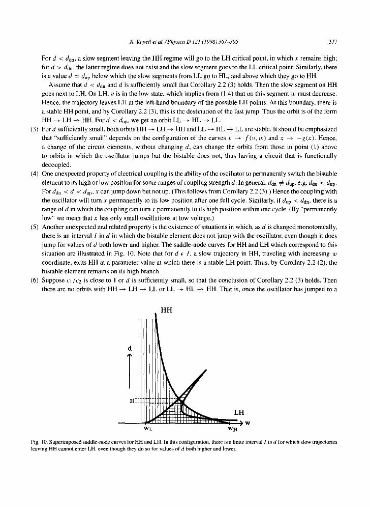
(5) Another unexpected and related property is the existence of situations in which, as d is changed monotonically, there is an interval I in d in which the bistable element does not jump with the oscillator, even though it does jump for values of d both lower and higher. The saddle-node curves for HH and LH which correspond to this situation are illustrated in Fig. 10. Note that for d ~ I, a slow trajectory in HH, traveling with increasing w coordinate, exits HH at a parameter value at which there is a stable LH point. Thus, by Corollary 2.2 (2), the bistable element remains on its high branch.

(6) Suppose cj /c2 is close to 1 or d is sufficiently small, so that the conclusion of Corollary 2.2 (3) holds. Then there are no orbits with HH ~ LH --+ LL or LL ~ HL --+ HH. That is, once the oscillator has jumped to a

HH

d

T l l - -

WL

L H I [ l l L l l l l l L I I I I I I I l l q " l ~ l l h " a ~ W

WH

Fig. 10. Superimposed saddle-node curves for HH and LH. In this configuration, there is a finite interval I in d for which slow trajectories leaving HH cannot enter LH, even though they do so for values of d both higher and lower.

378 N. Kopell et aL/Physica D 121 (1998) 367-395

d

SSL

H H

I l l l l l l l l l l l [ l l l l l l

wit ~ w

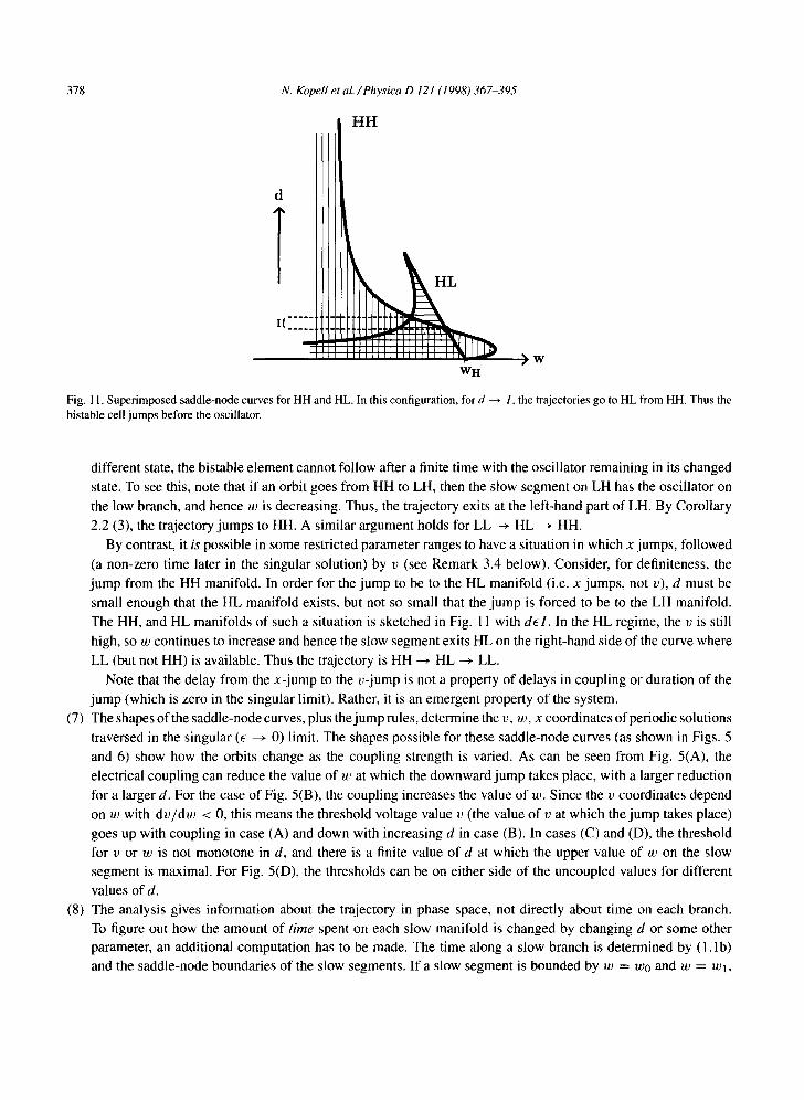
Fig. 11. Superimposed saddle-node curves for HH and HL. In this configuration, for d ~ 1, the trajectories go to HL from HH. Thus the bistable cell jumps before the oscillator.

different state, the bistable element cannot follow after a finite time with the oscillator remaining in its changed state. To see this, note that if an orbit goes from HH to LH, then the slow segment on LH has the oscillator on the low branch, and hence w is decreasing. Thus, the trajectory exits at the left-hand part of LH. By Corollary 2.2 (3), the trajectory jumps to HH. A similar argument holds for LL ~ HL --+ HH.

By contrast, i t /s possible in some restricted parameter ranges to have a situation in which x jumps, followed (a non-zero time later in the singular solution) by v (see Remark 3.4 below). Consider, for definiteness, the jump from the HH manifold. In order for the jump to be to the HL manifold (i.e. x jumps, not v), d must be small enough that the HL manifold exists, but not so small that the jump is forced to be to the LH manifold. The HH, and HL manifolds of such a situation is sketched in Fig. 11 with dEl. In the HL regime, the v is still high, so w continues to increase and hence the slow segment exits HL on the right-hand side of the curve where LL (but not HH) is available. Thus the trajectory is HH --~ HL ~ LL.

Note that the delay from the x-jump to the v-jump is not a property of delays in coupling or duration of the jump (which is zero in the singular limit). Rather, it is an emergent property of the system.

(7) The shapes of the saddle-node curves, plus the jump rules, determine the v, w, x coordinates of periodic solutions traversed in the singular (~ --~ 0) limit. The shapes possible for these saddle-node curves (as shown in Figs. 5 and 6) show how the orbits change as the coupling strength is varied. As can be seen from Fig. 5(A), the electrical coupling can reduce the value of w at which the downward jump takes place, with a larger reduction for a larger d. For the case of Fig. 5(B), the coupling increases the value of w. Since the v coordinates depend on w with dv /dw < 0, this means the threshold voltage value v (the value of v at which the jump takes place) goes up with coupling in case (A) and down with increasing d in case (B). In cases (C) and (D), the threshold for v or w is not monotone in d, and there is a finite value of d at which the upper value of w on the slow segment is maximal. For Fig. 5(D), the thresholds can be on either side of the uncoupled values for different values of d.

(8) The analysis gives information about the trajectory in phase space, not directly about time on each branch. To figure out how the amount of time spent on each slow manifold is changed by changing d or some other parameter, an additional computation has to be made. The time along a slow branch is determined by (1. lb) and the saddle-node boundaries of the slow segments. If a slow segment is bounded by w = wo and w = wt,

N. Kopell et al. / Physica D 121 (1998) 367-395 379

then (1. l b) implies that the time to traverse that segment is given by

/ *

T : ] [ 1 / E h ( v , w)]dw, (2.2) 71!(I

where v = v ( w , d) is the v-coordinate of the branch of critical points on that slow segment. As can be seen from (2.2), the time depends not only on w0 and wl but also on v(w, d), which in turn depends

on information not in the saddle-node curves. In some important cases, however, h (v, w) is essentially independent of v. For example, in the Morris-Lecar equations, h(v , w) has the form

h(v , w) = W~c(V) - w, (2.3)

where w = woo(v) is a saturating sigmoidal function as in Fig. 2. For v in the range of the slow segments of the periodic trajectory, woo(v) can almost be constant in v.

For such cases, we can read off from the saddle-node curves how the time on a given slow segment changes with d. For example, in Fig. 7 both boundaries of the slow segment move outward as d increases; this implies that the time on the HH slow segment increases with d. In Fig. 5(C) and (D), depending on the shape of the LL saddle-node curves, there can be afinite value of d at which the periodic trajectory is held longest on the HH slow segment.

The same analysis holds in establishing the effects of changing the equations. If f and/or g is changed without changing h, the time on a segment is again given by (2.2), with boundaries given by the saddle-node curves. If h is again independent of v in the relevant regions, the change of shape of the saddle-node curves changes the time on the slow segments in a predictable manner. We return to this theme in Section 5, where we show how changes in ionic currents of the bistable element change the shapes of the saddle-node curves, and hence affect the duty cycle.

In the previous part of this section, we have assumed that the surface h = 0 does not intersect the surface HH, LL, LH or HL of critical points of (1.3). If there is such an intersection, in general it will be a curve in v, x, w, d space. Such a point corresponds to a critical point for the full system (1.2). Thus, a slow trajectory approaching such a point will stop, and there will be no oscillation.

3. Equations and the saddle-node curves

In this section, we give results that connect the shapes of the curves v --> f ( v , w), x ~ - g ( x ) and their placement to the shapes of the saddle-node curves (or, more specifically, the projection to the d, w plane of the boundaries of the sets of stable critical points of (1.2)). We start with the HH saddle-node curve; the results and proofs for the LL curve are similar.

Theorem 3.1 below gives conditions that lead to the saddle-node curves in Fig. 5. As we will see, for d small, the behavior is determined just by the positions of VH and XH (as in Fig. 12). But for larger d, more global aspects of the graphs v ~ . f (v , w) and x ~ - g ( x ) come into play. Before we state the theorem, whose formal proof is in Section 4.4, we discuss its central ideas.

We can prove directly (Lemma 4.1) that the saddle-node curves are smooth except at isolated points, and they can be parametrized by d. However, the proof of that iemma does not provide information about the shapes of the saddle-node curves. To determine this, we construct the surface of stable critical points for which the HH curve is the boundary.

To construct the curve of saddle-nodes, we consider vertical slices in the d, w plane. We look for the (w-dependent) set o f d within each slice for which there are HH critical points; the boundaries of these sets form the curve d = d ( w )


A)

v----) f ( v , w ) I x--- ) - g ( x )

I !

v ~ x

v--) f(v,w)

B) ,' I

J

! x ---) - g ( x )

v ~ x

Fig. 12. Parts of a curve v --+ f ( v , w) and x ~ - g ( x ) . A critical point of (1.3) corresponds to a pair (v, x) for which f ( v , w) = - g ( x ) . The value of d for which that pair is a critical point is the aspect ratio (height/width) of the box drawn in figures A and B.

that we seek. The visual technique we use exploits the fact that, for a critical point of (1.3), the x and v coordinates must satisfy f (v, w) = - g ( x ) . Furthermore,

d = f ( v , w ) / ( v - x) = g ( x ) / ( x - v). (3.1)

Thus, a critical point of (1.3) with a given w can be visualized by drawing v ~ f ( v , w) and x ~ - g ( x ) on the same graph, with v, x on the same axis (Fig. 12); a solution corresponds to a pair of points (v, x) with f ( v , w) and g(x ) at the same height, and d is given by the aspect ratio (3.1) of the small rectangle in Fig. 12. Note that d > 0 implies that if v > x, then f ( v ) , - g ( x ) > 0, as in Fig. 12; if v < x, then f ( v ) , - g ( x ) < 0, as in Fig. 12.

A simple example is shown in Fig. 12 corresponding to solutions for all d > 0 (i.e. all aspect ratios); d = 0 corresponds to the pair of points on the v, x axis, and d --- oo to the point with x -- v. A more complicated situation is shown in Fig. 13, corresponding to values of w for which there are solutions only for some values of d. The key lemma (Lemma 4.3) says that the interval in d (for fixed w) can be parametrized by v or x; it can be constructed by continuation from a point known to correspond to a stable critical point of (1.3) up to a point at which d' (x) = 0 or d'(v) = 0. Lemma 4.2 says that such a point must be a saddle-node.

Fig. 13 shows a situation with OH > Xn, and some curves v ~ f ( v , w), w < WH filled in. At d = 0, there is a stable critical point for (1.3) with components x -- xH, and v = oH. For d > 0, the interval in d in which there are stable critical points can be parametrized by v, and this is indicated on each v ~ f ( v , w) curve as the darker interval. The value of d is computed for each point in the dark interval as the aspect ratio (3.1) of pairs of points (v, x) at the same height. The bullets not on the v- or x-axis correspond to points where d ' (v ) ---- 0. Note that the local maximum of the curve v --+ f ( v , w) is not in general the point at which d(v) reaches its local maximum; indeed, this can be seen from the geometry of the curves, as in Fig. 13, or by calculating the Jacobian of the right-hand side of (1.3), and seeing that the eigenvalues are strictly negative at the point at which v --~ f ( v , w) has its local maximum.

The geometrical construction of the w-dependent intervals in d is done separately for each w. It then remains to argue that the intervals can be put together to form a curve such as the ones in Figs. 5 or 6. Here the crucial point is that, by Lemma 4.1, the curve is known to be parametrized by d, i.e., each smooth piece of each of the curves is

N. Kopell et al . /Physica D 121 (1998) 367-395 381

x - - ) - g(x) w i n c r e a s i n g

!

v -9 f ( v . ~ ) - ~ / ~ ~ l . . v-) f(v..)_ 4 ~ ~ ~

S • • %

- " "

I ~, s

I

Fig. 13. Parts of curves v -* f ( v , w) and x --+ - g ( x ) in the case XH < OH. The curves v ~ f ( v , w) can be parametrized by v. The dark portion of each curve corresponds to the stable critical points for (1.3). At w = ~, the local maximum of v ~ f ( v , (o) intersects x ~ - g ( x ) . These curves are schematic, as are the dark portions and the bullets.

A) I

s ~ V ~ X x ~ l t • % X L s "

• ~ V ~ X

x - - ) - g (x) f(v.w~ ) f(v.w*)

B) x--)- g(x) I

s

X L d S %% V H ~ X 11][,,,/'J V X 9

t v - - ) f ( v , w . ) ~ ,, s

v - ~ f ( v , ~ v ) - - / ~ ~ "" v - ~ f ( v , ~ ) J I "

Fig. 14. Some schematic curves v ~ f ( v , w) in the case that XH > OH. For pairs (v, x) such that f, - g < 0, the requirement that d > 0 forces v < x. As w increases, the curves v -* f ( v , w) pull off the graph of x ~ - g ( x ) on the right-hand branch (A) or the middle branch (B) ofx -* - g ( x ) .

the graph of a funct ion w = w ( d ) . This creates constraints on the curves in d, w plane and forces the intervals to fit together in ways shown in Figs. 5 and 6.

Us ing these techniques, we can prove the fol lowing:

T h e o r e m 3.1. (i) Suppose that XH < VH and, as w decreases f rom w = WH, the curves v ~ f ( v , w ) intersect the right branch of

x ~ - g ( x ) . Assume that, as some value ~ of w, the intersection is at the local m a x i m u m of v ~ f ( v , w ) . (see Fig. 13.) Then the associated saddle-node curve is quali tat ively like that in Fig. 5(A). The vert ical asymptote occurs for a value of w greater than tb.

(ii) Suppose XH > VH and, as w increases f rom wH, there is a value w* such that the curve v - * f ( v , w ) is tangent to the right branch of x ~ - g ( x ) (see Fig. 14(A)). Then the associated saddle-node curve is qual i tat ively like

that in Fig. 5(B). The asymptote is at w = w*.

382

(iii)


Suppose that xH > VH and, as w increases from WH, there is a value of w such that the curve v -+ f ( v , w) is tangent to x -+ - g ( x ) along the middle branch of the latter. Suppose that as w increases further, the local maximum of v ~ f ( v , w) decreases below the local minimum of x -+ - g ( x ) (see Fig. 14(B)). Then the saddle-node curve is as in Fig. 5(C) or (D). In particular, it takes its maximum in w at a finite value of d. The maximum occurs at the value ~ of w for which the local max of v --+ f ( v , w) equals the local min of x -+ - g ( x ) . The asymptote of the saddle-node curve may be larger than WH (as in Fig. 5(C)) or less than WH (Fig. 5(D)). The asymptote occurs at a value w* of w larger than ~ , where ~ is such that v ~ f ( v , w) intersects the minimum o f x ~ - g ( x ) . Fig. 14(B) corresponds to the case w* > WH.

Remark 3.1. The behavior of the saddle-node curves for d small is intuitively clear. At d = 0 the saddle-node point is at w = WH, where v -+ f ( v , w) has its local max at f = 0. The x-component at d = 0 is xH, the high stable critical point. For 0 < d << 1 the slope of the saddle-node curve is determined by whether the v- or x-component is larger at d = 0; if, e.g. (as in Fig. 13) the v component is larger, then the electrical coupling pulls the v-component downward and causes the jump to the low voltage state at a lower value of w. The behavior for large d is much less intuitive.

Remark 3.2. Theorem 3.1 gives information about how the value of w at the saddle-node curve changes with d. The same techniques show how that value of w changes as the functions v --~ f ( v , w) and x -+ - g ( x ) change for fixed d. We return to this in Section 5, in which we show how changing g ( x ) can change the saddle-node curves.

Remark 3.3. The above techniques can be used to see the effects on the saddle-node curves of changing the relative proportions of the surface areas of the two cells. Going back to Eq. (1.2), expressed in terms of ~'l, f , ~', and p, it is possible to see that, for p2 > pl (i.e. increased proportion of surface area of the oscillator), the HH curve is moved toward WH. This agrees with the intuition that a smaller surface area for the bistable cell relative to the oscillator makes it more difficult for the bistable cell to change the point at which the oscillator jumps to the lower voltage (which is WH when there is no coupling). A similar statement holds for the LL curves. Conversely, for larger p, the pinning effect of the electrical coupling is larger.

Remark 3.4. Each case of Theorem 3.1 describes a set of hypotheses about the curves v ~ f ( v , w) in relation to x -+ - g ( x ) . It is possible to construct a family v ~ f ( v , w) whose behavior combines elements of the hypotheses of (i)-(iii), e.g., satisfying one of these for w small and another for w larger. Though the specific conclusions of Theorem 3.1 do not hold for such combinations, the methods in the proof remain valid, and can be used to find the saddle-node curves for arbitrary families v --+ f ( v , w) .

The next theorem describes the LH saddle-node curve; similar results hold for the HL curve. As will be shown in Section 4.1, all the saddle-node curves are piecewise smooth and parametrized by d. In addition, we have:

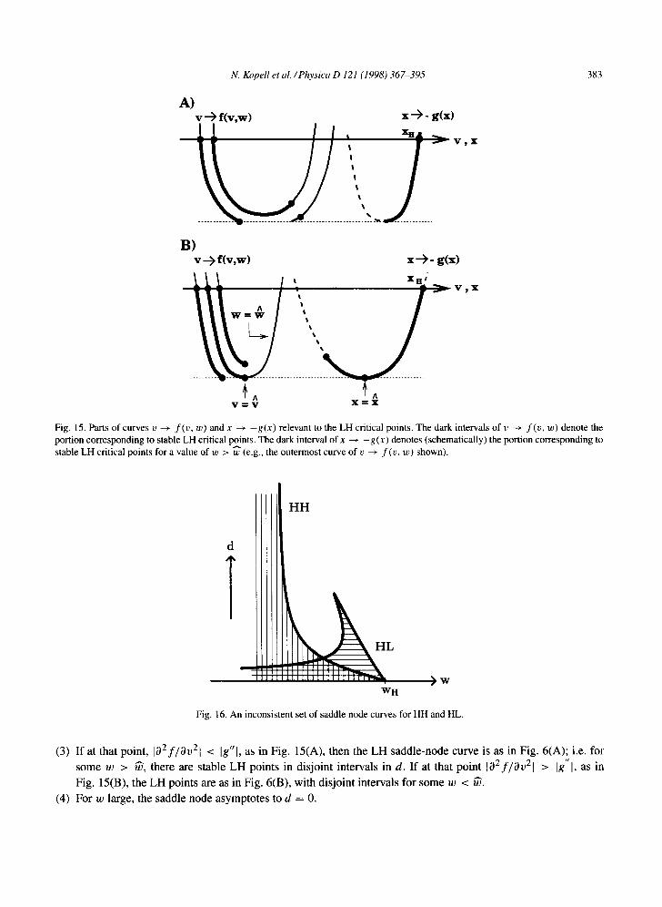
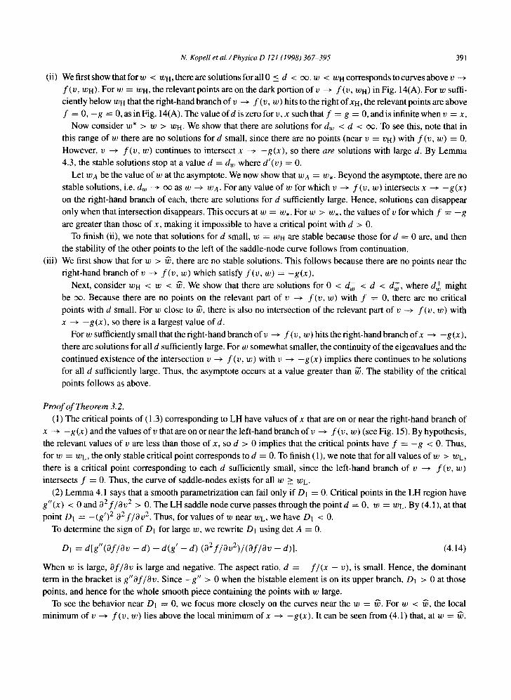
Theorem 3.2. the value o f x at which the local minimum o f x ~ - g ( x ) occurs (see Fig. 15). Then (1) The LH saddle-node curve extends for all values of w > WL. (2) Smooth parametrization fails only for points at which Dl = 0, where

Ol -~ d g ' [ O f /Ov - d] - [g' - d]Z[oZ f /Ov2].

Assume that for each w, the value v at which the local minimum of v ~ f ( v , w) occurs is less than

(3.2)

For w small, Dj < 0, for w large Dt > 0. Thus, there is a point at which D1 = 0. Let ~ be the value of w and @, x~ the values of (v, x) such that f (U, N) = - g ( x ~ and Of/Or = 0, g ' = 0. If at ~ , ~', ~', we have 0 2 f / O v 2 = - g " , then Di = 0 at that point.

N. Kopell et al . /Physica D 121 (1998) 367-395 383

A ) v --') f ( v , w ) x " ) - g ( x ) ~ v ~ x

B ) v --> f ( v , w ) x --') - g ( x )

~ 1 ~ I , x~, v ~ x

v ~ - v x m x

Fig. 15. Parts of curves v --+ f ( v , w) and x ~ - g ( x ) relevant to the LH critical points. The dark intervals of v ~ f ( v , w) denote the portion corresponding to stable LH critical points. The dark interval o f x --~ - g ( x ) denotes (schematically) the portion corresponding to stable LH critical points for a value of w > ~ (e.g., the outermost curve of v --+ f ( v , w) shown).

IIIII

d

T H H

~ H L

i ~ I I I I I I i i i i ,,r,m-,~.~. 1 1 I I I I I

W H ) w

Fig. 16. An inconsistent set of saddle node curves for HH and HL.

(3) If at that point, 102f/Oo2l < Ig"l, as in Fig. 15(A), then the LH saddle-node curve is as in Fig. 6(A); i.e. for t t

some w > O, there are stable LH points in disjoint intervals in d. If at that point 102f/Ov21 > Ig I, as in Fig. 15(B), the LH points are as in Fig. 6(B), with disjoint intervals for some w < O.

(4) For w large, the saddle node asymptotes to d -- 0.


x ~ - g ( x )

"/li e

xi 7 ¢ N , \ ," xH ) V~X

Fig. 17. Curves v ~ f ( v , w) and x ~ - g ( x ) that give rise to the saddle-node curves in Fig. 11.

Remark 3.5. The saddle-node curves HH, LH, HL and LL are partially, but not totally independent of one another. (By independent we mean that, given the curves, functions f and g can be constructed that have those curves.) As can be seen from the statements of Theorems 3.1 and 3.2, different parts of each of the saddle-node curves depend on different aspects of the functions v ~ f ( v , w) and x ~ - g ( x ) . There is an overlap, however. Consider, for example, Fig. 16; which has an HH curve that is decreasing in w as d increases. This pair of saddle-node curves is not achievable for any choice of f and g. The reason is essentially that both the HH and HL saddle-nodes depend on the shape of v ~ f ( v , w) on their right-hand branches. For d small, the relevant stable points of HH have x-components that lie much to the right of the x-components of the points of HL; this forces the saddle-node curves HH to lie to the right of the HL curve, contradicting Fig. 16. Fig. 11 however, is achievable. Functions f and g with the appropriate qualitative properties necessary to produce Fig. 11 are given in Fig. 17. We leave to the reader the exercise of verifying this last assertion; practice in going between functions such as in Fig. 17 and the associated saddle-node curves can be obtained by going through the proofs of Theorems 3.1 and 3.2 in Section 4.4.

Remark 3.6. The configuration in Fig. 11 is compatible with the sequence of jumps HH ~ LH ~ HH, in which the oscillator jumps down, then up again, leaving the bistable on its high branch. To be certain that the HH piece of the trajectory next enters HL instead of LH, we can arrange that the right hand boundary of the LH saddle-node curve fall below the bottom of the interval I. This can be done because that part of the curve depends on the position of the left branch of v ~ f ( v , w) , which can be manipulated independently of the parts of these curves that determine the HH curve and HL curve.

Remark 3. 7. The techniques of the proof again give results about the effects of changing p. As before, increasing p changes the saddle-node curve in the direction of decreasing the pinning effect of the bistable cell.

4. Proofs

4.1. The saddle-node curves

We start by showing (Lemma 4.1) that there are four saddle-node curves as described in Section 2.1. This allows us to see that the LL and HH curves exist for all d. Then we show (Lemma 4.2) that the ends of the slow segments lie on the saddle-node curves. Lemma 4.3 gives the critical characterization of the saddle-node points, which allows us to read offthe saddle-node curves from the curves v ~ f ( v , w) and x --~ - g ( x ) . Finally, Lemma 4.4 gives the condition for a saddle-node to be non-degenerate, which we use in deducing the rules for jumping from one slow segment to another.


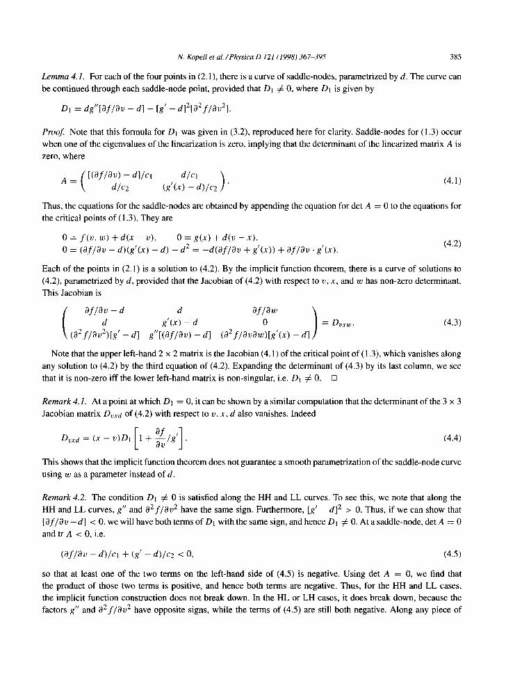
Lemma 4.1. For each of the four points in (2.1), there is a curve of saddle-nodes, parametrized by d. The curve can be continued through each saddle-node point, provided that Dl # 0, where D1 is given by

D1 = d g ' [ O f /Ov - d] - [ f - d]2[O2 f /Ov2].

Proof Note that this formula for Dt was given in (3.2), reproduced here for clarity. Saddle-nodes for (1.3) occur when one of the eigenvalues of the linearization is zero, implying that the determinant of the linearized matrix A is zero, where

A = ( [ ( O f / O r ) - d]/cl d / c l ) (4.1) \ d/c2 (g'(x) - d) /c2 "

Thus, the equations for the saddle-nodes are obtained by appending the equation for det A = 0 to the equations for the critical points of (1.3). They are

0 = f ( v , w) + d(x - v), 0 = g(x) + d(v - x) , 0 = (Of/Ov - d ) ( f ( x ) - d) - d 2 = - d ( O f / O p + g '(x)) + Of/Oo. g'(x) . (4.2)

Each of the points in (2.1) is a solution to (4.2). By the implicit function theorem, there is a curve of solutions to (4.2), parametrized by d, provided that the Jacobian of (4.2) with respect to v, x, and w has non-zero determinant. This Jacobian is

( O f / O d - d d O f /Sw ) g ' (x) - d 0 = Dvxw. (4.3)

\ (oz f /OvZ)[g - d] gr'[(Of/Ov) - d] (02 f /avOw)[g ' ( x ) - d]

Note that the upper left-hand 2 x 2 matrix is the Jacobian (4.1) of the critical point of ( 1.3), which vanishes along any solution to (4.2) by the third equation of (4.2). Expanding the determinant of (4.3) by its last column, we see that it is non-zero iff the lower left-hand matrix is non-singular, i.e. D1 5 ~ 0. []

Remark 4.1. At a point at which D1 = 0, it can be shown by a similar computation that the determinant of the 3 x 3 Jacobian matrix Dvxd of (4.2) with respect to v, x, d also vanishes. Indeed

O f , ,] Dvxd = (x - v )Dj l + ~ v / g j . (4.4)

This shows that the implicit function theorem does not guarantee a smooth parametrization of the saddle-node curve using w as a parameter instead of d.

Remark 4.2. The condition Dl # 0 is satisfied along the HH and LL curves. To see this, we note that along the HH and LL curves, g" and 02 f /Ov 2 have the same sign. Furthermore, [g' - d] 2 > 0. Thus, if we can show that [Of/8 v - d] < 0, we will have both terms of D1 with the same sign, and hence D1 # 0. At a saddle-node, det A = 0 and tr A < 0, i.e.

(Of~Or - d ) / c l + (gl _ d)/c2 < O, (4.5)

so that at least one of the two terms on the left-hand side of (4.5) is negative. Using det A = 0, we find that the product of those two terms is positive, and hence both terms are negative. Thus, for the HH and LL cases, the implicit function construction does not break down. In the HL or LH cases, it does break down, because the factors g" and 8 e f / o v 2 have opposite signs, while the terms of (4.5) are still both negative. Along any piece of


the LH curve which is smoothly parametrized by d, the sign of D1 does not change, a fact that will be used in Section 4.4.

In general, critical points can lose stability either by a saddle-node bifurcation or a Hopf bifurcation. In the case of ( 1.3), only the first can happen, as shown in the next lemma.

Lemma 4.2. Along any curve of stable critical points of (1.3) in v, x, d, w space, the critical point does not encounter a Hopf bifurcation before it encounters a saddle-node.

Proof A critical point (v, x) of (1.3) is stable iff the matrix (4.2) has negative eigenvalues. At a boundary of stability given by saddle-nodes, one of the eigenvalues is zero, so the determinant must vanish. The determinant is

Det a -- [(Of/Or - d)(g' (x) - d) - d2]/clc2 = [ - d ( O f / O v + g ' (x)) + Of~Or. g'(x)]/ClC2. (4.6)

Hopf bifurcations occur where the eigenvalues are pure imaginary, i.e. where the trace of the Jacobian determinant is zero and the determinant is positive. Thus, for (4.1) the conditions for a Hopf to occur first are Tr A = 0 and det A > 0. Using Tr A = 0 we have det A = - (Cl /C2)(g t - d) 2 - d 2 < 0. This contradicts encountering a Hopf bifurcation before a saddle-node. []

We now go to the key lemma. For a fixed value of d, the construction of a singular periodic orbit involves finding the values of w at which a slow segment hits a saddle-node boundary curve. The geometric construction (discussed briefly in Section 3) for getting the S-N curves from the functions f and g does not allow us to find those points directly. In that construction, we fix w and find the values of d that lie on the boundary curves. Each of these vertical "slices" in the d - w plane is more conveniently parametrized by v and/or x than by w, with d = d(v) or d = d(x) . The following lemma characterizes the saddle-node points as those for which the function d = d(v) or d = d(x) (along a "slice" w = constant) has a local maximum or minimum. This characterization is the heart of the geometrical construction.

Lemma 4.3. For any fixed w, there is an interval (perhaps empty or a single point) in d >_ 0, parametrized by v and/or x, for which there are stable critical points for (1.3). Each of these curves of critical points (in v, x, d, w space) can be parametrized by v (resp. x), providing the curve does not touch a point at which g~(x) = 0 (resp. Of(v, w) /Ov # 0) or the set v = x. If the curve is parametrized by v (i.e., is described by v, x (v ) , d(v)) , then the critical point ~, x (~), d(~) is a saddle-node if and only if d ~ (~) = 0. For a curve parametrized by x the critical point 2, v(2), d(2) is a saddle-node if and only if d'(-£) = O.

Proof. To see if a curve of critical points in v, x, d, w space can be parametrized by v (with w fixed), we consider the Jacobian matrix of (1.3) with respect to d and x. The determinant of this matrix is (1 /c l c2)(v - x)g1(x). Thus the curve can be parametrized by v away from the points at which g~(x) = 0 or v = x. Similarly, for parametrization with respect to x, the determinant of the relevant Jacobian matrix is ( l / c l c2)(x - v)Of/Ov, so the parametrization is valid when this product is non-zero.

To find the saddle-node boundary, we write d = f ( v , w) / [v - x]. Then d'(v) = {(v - x ) O f / S v - f ( v , w) • (1 - x~(v))}/(v - x) 2. Differentiating 0 = g(x) + d(v - x), we find that 0 = g'(x)x~(v) + d[1 - x'(v)] or x ' (v ) = d / [d - g'(x)]. Substituting (v - x) = - g ( x ) / d into the formula for d'(v) we thus get

d ' ( v ) = O iff - g 8 f ( d ) d 8v f 1 d - g ' = 0 " (4.7)


At a critical point, we must have f = - g , so (4.7) reduces to [Of/Ov]/d - 1 + [d/(d - g'(x))] = 0. Sim- plifying this expression, we get that d(Of/Ov + g ' (x) ) = Of~Or • g', which says that the determinant of the Jacobian (4.1) is zero, so there is a saddle-node. An identical argument works if the curve is parametrized by x. []

Non-degenerate saddle-nodes have a half-plane of trajectories approaching the critical point, and a unique trajectory (unstable manifold) leaving the critical point. The following lemma implies that all the critical points on HH or LL are nondegenerate. For LH or LH, there are isolated degeneracies which coincide, if cl = c2, with the points at which the curve cannot be smoothly parametrized by d.

Lemma 4.4. The non-degeneracy condition for a saddle-node is (g' - d)D2 ~ 0, where

D 2 =~ dg" [(Of/Or) - d] [g' -- d]2(O2f /Ov 2) C2 Cl

Remark 4.3. Note that if cl ---- c2, then Dj = D2 up to a positive constant multiple.

(4.8)

Proof o f Lemma 4.4. Let e denote the eigenvector for the zero eigenvalue of some saddle-node, and Q the vector of quadratic terms in the Taylor expansion around the saddle node. The general non-degeneracy condition for a saddle-node is that Q(e, e) • e :fi O. In the case of (1.3), let (ev, ex) denote the components ofe. The vector Q(e, e) is given by [(O2f/Ov2)e2/2Cl, g"e2x/2C2]. Thus

O Z f e 3 / c l g ' te3/c2 . (4.9) 2 Q ( e , e ) . e = ~ v 2 ~,, +

Now e~ and ex can easily be computed (up to a constant) from (4.1). In particular, we may take (e~,, ex) to be (d - g' , d), which points in the first quadrant. We may then rewrite (4.9) as

oZ f (d 2Q(e, e) • e = ~ - g ' )3 /c I + g 'd3 /c2 . (4.10)

Using det A = 0 along a saddle-node, we have that 2Q(e, e ) . e = (g' - d)D2. []

4.2. A proper~ o f the slow segments

We now show that along any given slow segment, the variables v and w = w(v) satisfy d v / d w < 0. This implies that the projection of the trajectory to the v, w plane is qualitatively like the outer branches of the v' = 0 nullcline in Fig. 2.

The critical points of (1.2) satisfy the first two equations of (5.2). Differentiating with respect to w, we get the equations

( ( 1 A d x / d w =

where A is given in (4.1). (Note that, since we are concerned with critical points of (5.2), the scaling factors cl, c2 play no role.) At a stable critical point, the eigenvalues of A are negative. To find the sign of dv /dw , we solve (4.11):

d x / d w ] -- d ~ A - d O f / O v - d " (4.12)


Hence, d v / d w = - ( 1 / d e t A) Of/Ow (g'(x) - d). Since det A > 0 and Of/Ow < 0, we find that sign d v / d w = sign (g' - d). To determine the latter, we note that (4.5) is valid since the eigenvalues are both negative. Hence, as in Remark 4.2, at least one of the terms is negative. Using (4.5), (4.6) and det A > 0, we get that both (Of~Or - d) and (g' - d) are negative.

4.3. The destination o f the fas t jumps and some consequences

We now prove the assertions made in Section 2.2, including Theorem 2.1. The proof requires some information about the geometry of the fast equations near a non-degenerate critical point. At a non-degenerate saddle-node (~, 2) there is a half-plane of trajectories that approach the saddle-node as t --~ ~ , and a unique (unstable manifold) trajectory that approaches the critical point as t -+ - ~ (see Fig. 8). We first show that the unstable manifold must be in the first or third quadrants generated by (~, ~-).

Lemma 4.5. Let (~, Y) denote a non-degenerate saddle-node of (1.3). (i) The eigenvector associated with the zero eigenvalue of (~, 2) has positive slope (i.e. is in the first and third

quadrants). (ii) Let D2 be as in (4.8). Then the unstable manifold trajectory is in the first quadrant if D2 < 0 and in the third

quadrant if D2 > 0.

Proof (i) The eigenvector (d - gt, d) of (4. l) corresponding to the zero eigenvalue has a slope

(d - Of / O v ) / d = d / ( d - g'). (4.13)

As in Remark 4.2, g ' - d and 3 f fOv - d are both negative, so that the slopes in (4.13) are positive. (ii) From the proof of Lemma 4.2, we know that 2 Q (e, e). e = (gt _ d) D2, so D2 has the opposite sign of Q (e, e). e.

The sign of Q(e, e ) . e says whether the unstable manifold is in the same or the opposite direction from the vector e. Hence, D2 < 0 (resp. D2 > 0) implies that it is in the same (resp. opposite) direction. Since (d - gl, d) points in the first quadrant, the conclusion follows. []

We now show that the unstable manifold of a non-degenerate critical point (~, 2) must tend to the neighboring critical point (_v, x). Let R denote the rectangle in v, x space bounded by v --= ~, x -= 2, v - v, x = x. The definition of neighboring given in Section 2 is equivalent to saying that (_v, x) is in the appropriate direction, and that there are no other critical points of (1.3) in 7?.. We may then restate Theorem 2.1 in a slightly stronger manner:

Theorem 2.1a. For Eqs. (1.3), any non-degenerate saddle-node has exactly one neighboring critical point. All trajectories in 7~ tend to that critical point; in particular, the unstable manifold tends to that point.

Proof We first show that there is at least one critical point in the appropriate quadrant. Note that, by the cubic nature of f and g, f ( v , w) and g(x) are bounded above uniformly for v -+ o¢, x -~ cx~ and bounded below uniformly for v -+ - c e , x -~ - o o . Suppose, for definiteness, the unstable manifold is in the third quadrant. It follows from (1.3) that, for v, x sufficiently negative, v' > 0 and x I > 0. Thus trajectories cannot go to infinity.

For any critical point ~, ~- (not just a saddle-node) the vector field of (1.3) points into the third quadrant on the lines v = ~ ,x < 2 and x = 2, v < ~. (This follows immediately from v r = 0, x r = 0 at v = ~ ,x = 2 and the form of the coupling.) Thus, the trajectories cannot leave the closure of the third quadrant or become unbounded. In a two-dimensional phase space, this implies that there is at least one critical point in the closure of the third


x i

.............................................. t t i t i i i l / " , :

~ V

(v,, x,)

(v,, x~)

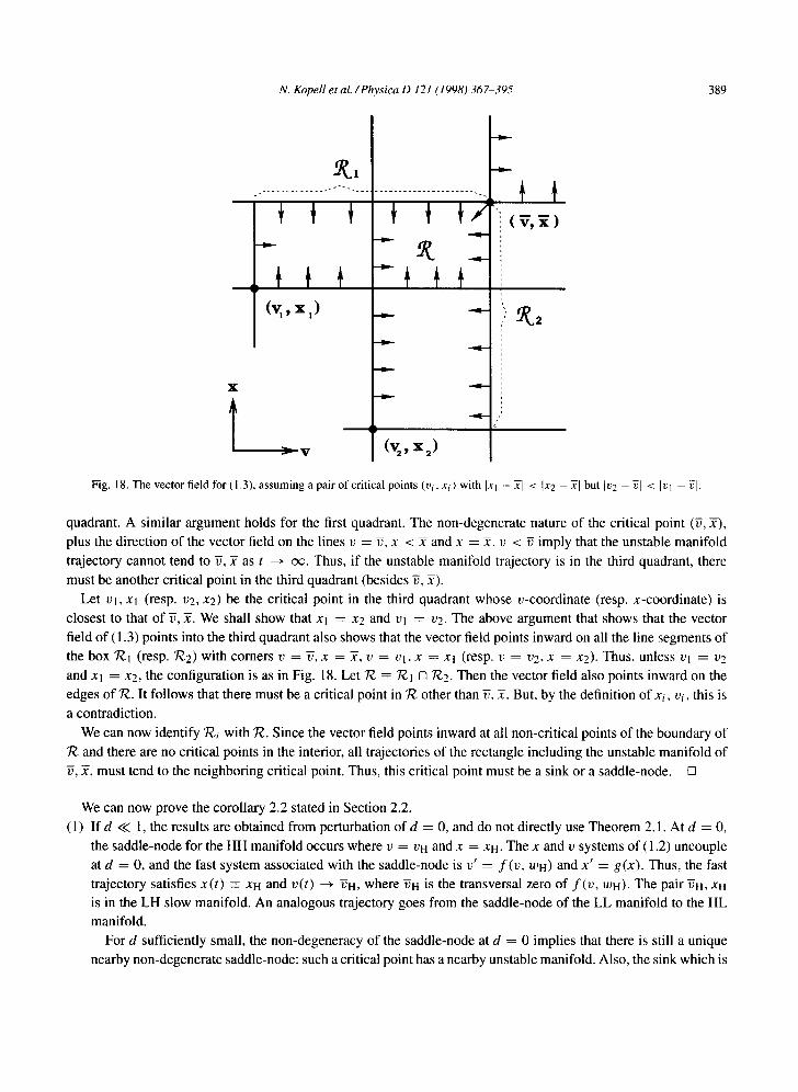
Fig. 18. The vector field for (1.3), assuming a pair of critical points (vi, xi) with Ixj - ~l < Ix2 - Y[ but Iv2 - ~l < IVl - ~l-

quadrant. A similar argument holds for the first quadrant. The non-degenerate nature of the critical point (~, Y), plus the direction of the vector field on the lines v = ~, x < Y and x = Y, v < ~ imply that the unstable manifold trajectory cannot tend to v, x as t ~ ~ . Thus, if the unstable manifold trajectory is in the third quadrant, there must be another critical point in the third quadrant (besides ~, Y).

Let Vl, Xl (resp. v2, x2) be the critical point in the third quadrant whose v-coordinate (resp. x-coordinate) is closest to that of ~, 2. We shall show that Xl = x2 and vl = v2. The above argument that shows that the vector field of (1.3) points into the third quadrant also shows that the vector field points inward on all the line segments of the box 7~1 (resp. 7~2) with comers v = ~, x = Y, v = Vl, x = xl (resp. v = v2, x = x2). Thus, unless Vl = v2 and Xl = x2, the configuration is as in Fig. 18. Let 7~ ----- 7~1 N 7~2. Then the vector field also points inward on the edges of R. It follows that there must be a critical point in 7~ other than ~, Y. But, by the definition of xi, vi, this is a contradiction.

We can now identify Ri with R. Since the vector field points inward at all non-critical points of the boundary of and there are no critical points in the interior, all trajectories of the rectangle including the unstable manifold of

v, x, must tend to the neighboring critical point. Thus, this critical point must be a sink or a saddle-node. []

We can now prove the corollary 2.2 stated in Section 2.2. (1) I f d << 1, the results are obtained from perturbation o f d = 0, and do not directly use Theorem 2.1. At d = 0,

the saddle-node for the HH manifold occurs where v = VH and x = XH. The x and v systems of ( 1.2) uncouple at d = 0, and the fast system associated with the saddle-node is v' -- f ( v , WH) and x ' ---- g(x) . Thus, the fast trajectory satisfies x ( t ) =--- xH and v(t) ~ ~H, where ~H is the transversal zero of f ( v , wH). The pair ~H, XH is in the LH slow manifold. An analogous trajectory goes from the saddle-node of the LL manifold to the HL manifold.

For d sufficiently small, the non-degeneracy of the saddle-node at d = 0 implies that there is still a unique nearby non-degenerate saddle-node; such a critical point has a nearby unstable manifold. Also, the sink which is


the t ~ ~ limit for d = 0 perturbs to a nearby sink with a nearby basin of attraction. Hence it is still true that the unstable manifold of the HH (resp. LL) saddle node goes to the LH (resp. HL) slow manifold. That is, for sufficiently small coupling, the oscillator changes its branch (between high and low) but the bistable element does not.

(2) Theorem 2.1 says that the unstable manifold of the HH saddle node must tend to the nearest critical point in the correct direction. By hypothesis, the LH or HL stable critical point is in the correct direction. Furthermore, the x-coordinate (resp. v coordinate) of the LH (resp. HL) critical point is closer to that of the HH critical point than that of the LL critical point. By Theorem 2.1a, if either coordinate is closer, so is the other. Thus, if an LH or HL stable critical point exists for a fixed w, d, the HH state at that w, d may not jump to the LL state.

(3) For definiteness, consider LH; the argument is the same for HL. For fixed d, there is a finite interval in w for which there are LH stable critical points (see Fig. 6). We focus on the end points w_ < w+ of the interval. Each end point corresponds to a saddle-node for (1.3). At a saddle-node, at least one of Of~Or and g~ must be positive, since the determinant of (4.1) is positive if both those quantities are negative. Indeed, for w < O, the saddle-node has Of/Or > 0, and for w > O, the saddle-node has g~ > 0. Thus, the end point with w = w_ (resp. w = w+) corresponds to a critical point of (1.3) with O f l a y > 0 (resp. gt > 0) (see Fig. 15). For the unstable manifold of a non-degenerate saddle-node to go to HH (resp. LL), its tangent must point into the first (resp. third) quadrant. By Lemma 4.5, the tangent points into quadrant 1 (resp. quadrant 3) if D2 < 0 (resp. D2 > 0). We also know that if cj/c2 = 1, then D2 = 0 implies DI = 0. Thus, for Cl/C2 sufficiently close to 1 (depending on d), sgn D2 = sgn DI at w = w_ and w ---- w+. We know that D1 > 0 for w > • by Theorem 3.2. Hence, for Cl/C2 close enough to 1, we have that D2 < 0 at w_ and D2 > 0 at w+. Hence, if the slow trajectory exits at w_, the trajectory goes to HH, and if it exits at w+, it goes to LL.

4.4. From geometry of equations to geometry of trajectories

Proof of Theorem 3.1. For each fixed w, we construct an interval of critical points for a range of d, with the end points established to be saddle-nodes of the fast system. The saddle-node curve we want is the union of the end points of those intervals. The stablity of the critical points to the left of the saddle-node curve is established by continuation, starting from some points known to be stable. For example it is easy to see from (4.1) that the four basic d = 0 solutions are stable, using the slopes of v ~ f ( v , w) and x ~ - g ( x ) at the points where f = 0 = g. From Lemma 4.2, any curve in w, d space that starts at a stable point and does not pass through the saddle-node curve has points that are the parameters for stable fixed points.

(i) First consider d << 1. For this case, there are no stable critical points for w > WH. To see this, we note that for w > wn, the points near v = OH on v ~ f ( v , w) are below the line f = 0. Recall that a critical point corresponds to a pair v, x with f ( v , w) = - g ( x ) and associated d = f / ( v - x). With f < 0, we must have (v - x) < 0 to have d > 0. But the points near OH = 0 on v ~ f ( v , w) are to the right ofxH.

For w < wH and close to wH, there is a part of v ~ f ( v , w) for which d = f / ( v - x) > 0. By continuity of stability, these are all stable for d sufficiently small. As proved in Lemma 4.3, the stability ends where d ' (v ) = 0. By direct calculation using (4.1), the point on a curve v -+ f ( v , w) satisfying Of~Or = 0 corresponds to a stable point, so the saddle node occurs at a lower value of v (see Fig. 13).

The asymptote occurs at the highest value of w for which there are solutions for all 0 < d < cx~. This value, w = w*, is the value at which the saddle-node point lies on the intersection of the curves v --+ f ( v , w) and curve x --+ -g ( x ) . If at some w = ~ , the local max of v --+ f ( v , ~) is on x ~ -g ( x ) , we have W * > ~ .


(ii) We first show that for w < 1/)H, there are solutions for all 0 < d < oc. w < to H corresponds to curves above v --+ f ( v , WH). For w = wn, the relevant points are on the dark portion of v ~ f ( v , WH) in Fig. 14(A). For w sufficiently below wn that the right-hand branch of v --+ f (v, w) hits to the right of XH, the relevant points are above f = 0, - g = 0, as in Fig. 14(A). The value o f d is zero for v, x such that f ---- g = 0, and is infinite when v = x.

Now consider w* > w > WH. We show that there are solutions for dw < d < c~. To see this, note that in this range of w there are no solutions for d small, since there are no points (near v = vn) with f ( v , w) = O. However, v ~ f ( v , w) continues to intersect x --~ - g ( x ) , so there are solutions with large d. By Lemma 4.3, the stable solutions stop at a value d = dw where d'(v) = O.

Let WA be the value of w at the asymptote. We now show that WA = W,. Beyond the asymptote, there are no stable solutions, i.e. d~ ~ o~ as w ~ ~/3 A. For any value of w for which v ~ f ( v , w) intersects x --+ - g ( x ) on the right-hand branch of each, there are solutions for d sufficiently large. Hence, solutions can disappear only when that intersection disappears. This occurs at w = w.. For w > w. , the values of v for which f = - g are greater than those of x, making it impossible to have a critical point with d > 0.

To finish (ii), we note that solutions for d small, w = wrt are stable because those for d = 0 are, and then the stability of the other points to the left of the saddle-node curve follows from continuation.

(iii) We first show that for w > O, there are no stable solutions. This follows because there are no points near the right-hand branch of v ~ f (v, w) which satisfy f (v, w) = - g ( x ) .

Next, consider wn < w < O. We show that there are solutions for 0 < d~ < d < d +, where d + might be oo. Because there are no points on the relevant part of v ~ f ( v , w) with f = 0, there are no critical points with d small. For w close to O, there is also no intersection of the relevant part of v -9, f ( v , w) with x ~ - g ( x ) , so there is a largest value of d.

For w sufficiently small that the right-hand branch of v --+ f (v, w) hits the right-hand branch o fx ~ - g (x), there are solutions for all d sufficiently large. For w somewhat smaller, the continuity of the eigenvalues and the continued existence of the intersection v --+ f ( v , w) with v ~ - g ( x ) implies there continues to be solutions for all d sufficiently large. Thus, the asymptote occurs at a value greater than ~ . The stability of the critical points follows as above.

Proof of Theorem 3.2. (1) The critical points of (1.3) corresponding to LH have values of x that are on or near the right-hand branch of

x --+ - g (x) and the values of v that are on or near the left-hand branch of v --+ f (v, w) (see Fig. 15). By hypothesis, the relevant values of v are less than those of x, so d > 0 implies that the critical points have f = - g < 0. Thus, for w = WL, the only stable critical point corresponds to d = 0. To finish (1), we note that for all values of w > WL, there is a critical point corresponding to each d sufficiently small, since the left-hand branch of v ~ f ( v , w) intersects f = 0. Thus, the curve of saddle-nodes exists for all w > WL.

(2) Lemma 4.1 says that a smooth parametrization can fail only if D1 = 0. Critical points in the LH region have g"(x) < 0 and 02f /Ov 2 > 0. The LH saddle node curve passes through the point d = 0, w = WL. By (4.1), at that point D1 = _(g , )2 ozf/ov2. Thus, for values of w near WL, we have Dl < 0.

To determine the sign of Dl for large w, we rewrite D1 using det A = 0.

Ol = d[g" (Of /Ov - d) - d(g' - d) (oz f / ov2 ) / (O f /Ov - d)]. (4.14)

When w is large, Of~Or is large and negative. The aspect ratio, d = - f / ( x - v), is small. Hence, the dominant term in the bracket is g"Of/Ov. Since - g " > 0 when the bistable element is on its upper branch, D1 > 0 at those points, and hence for the whole smooth piece containing the points with w large.

To see the behavior near D1 = 0, we focus more closely on the curves near the w = O. For w < O, the local minimum of v --+ f ( v , w) lies above the local minimum o f x ~ - g ( x ) . It can be seen from (4.1) that, at w = O,


the associated point ~', ~ corresponds to a saddle-node. Suppose that at 3 , ~', ~ we have 0 2 f / O v 2 : - g " . From (3.2), we have

DI = - d Z g '' - d 2 oz f /ov 2 : O.

(3) The pairs of points (x, v) with f = - g , Of~Or < 0 and _g l > 0 correspond to stable critical points. As in the HH case, there are also some points with Of~Or > 0 or - g < 0. The stability of a pair depends on the sign of det A = Of~Or. g' - d[Of/Ov + g']. For points near v = ~, x = Z, the dominant term in det A is - d [ O f / O v + g'].

First suppose that [oZf/ov21 < gt,, as in Fig. 15(A). Then for pairs near ~', ~" satisfying f ( v , 3 ) = g(x), the curvature implies that IOf/Ov[ < Ig'l. It follows that there are some stable points with v > ~" and x > ~" (see Fig. 15(A)). By continuity, for w > ~ (but close enough) there are also points with v > ~', x > ~" satisfying f ( v , w) = - g ( x ) and the stability condition. These give rise to values of d in an interval disjoint from the set of d ' s associated with v < ~'.

Now suppose 102f/Ov21 > g,t, as in Fig. 15(B). This time, at w ---- 3 , the stability criterion is satisfied for points with v < ~', x < ~'. For w < ~ (but close enough) continuity again implies there are stable solutions with v < ~" and x < ~'. As above, the associated set of d 's for these solutions lie in an interval disjoint from that corresponding t ox > x .

(4) As w increases, the left-hand branch of the curve v --+ f ( v , w) moves to the left, further from x -+ - g ( x ) . At the saddle-node, If[ is bounded by J min g (x)l, where the minimum is taken over the points of the middle and fight branches o fx ~ - g ( x ) (see Fig. 15). Since d = - f / ( x - v), and the numerator is bounded while the denominator increases without bound, we have that d --~ 0 as w increases.

5. Discussion

5.1. A geometric look at duty cycle regulation

The analysis in this paper was motivated partly by the simulations in [2] concerning the regulation of "duty cycle", described in Section 1. When current is injected into the oscillator cell ("AB cell"), the period of the cell changes, mainly by a change in the time the cell is quiet. Thus, the proportion of time the cell is bursting (the duty cycle) changes with injected current. When the cell is coupled to the bistable element ("PD cell"), the resulting network is able to keep a fairly constant duty cycle. Abbott et al. [2] suggested a mechanism involving a slowly changing current added to the PD cell. In that model, the maximum conductance ~ of the current increases linearly on the active branch and decreases linearly on the other branch; equilibrium occurs at a value of ~ for which the change over a full cycle is zero. Abbott et al. [2] showed that for a linear change in the slow conductance, the duty cycle is independent of the injected current in the AB cell.

The geometry in this paper does not say more about the mechanism for the regulation. Rather, it sheds light on how a change of properties of the bistable element can change the time on the active part of the cycle enough to balance the changes in the inactive part, so as to maintain the constant burst proportion. It also shows why the equilibrium produced by this method is stable.

Over one cycle, ~ is almost a constant. Thus, to consider its effects, we replace the third equation of (1.2) by

C2 dx / dt = g(x) + -~G(x). (5.1)

Here, x --> G(x) is qualitatively as in Fig. 19(A), with a zero at a lower value than the lowest critical point of x' = g(x) and negative for x larger than that value. The new current is ~G(x) . By including some of the term -~G(x) in the definition of g(x), we can, with no physical contradiction, allow ~ to be negative as well as positive.


A)

393

• --~ G(x) ~ x . ,

B) x---~ - g(x) ~ Z

S S

S

Fig. 19. (A) Graph of x ~ - G ( x ) . (B) Graphs of x ~ - g ( x ) and x ~ -lg(x) + ~G(x)] for two values of ~, one positive and one negative. The graph of x --~ - [g (x) + ~G (x)] is obtained from that of x -~ - g (x) by pivoting the latter around a point near its left zero. For ~ > 0, the points to the right of the pivot point are moved upward.

Changing the value of ~ can then be thought of as modulating the conductance of an outward current with a low reversal potential. The graphs of x ~ - g ( x ) and x --+ - g ( x ) + -~G(x) are as in Fig. 19(B) for a pair of values of ~, one positive and one negative. We also assume that h is chosen so that the speed w' is relatively independent of the value of v on each of the branches (see Section 2.3).

For ~ > 0, the graph of x ~ - [ g ( x ) + ~G(x)] is perturbed from that of x ~ - g ( x ) by being pivoted upward around the point x -- x0. Since the pivot point is near the lower critical point XL, the choice of ~ has only a small effect on the length of time spent on the lower branch. Thus, we focus on the time spent on the high (HH) branch.

In the context of the example of [2], we are interested in d large enough so that there are no HL or LH stable critical points. Hence, we restrict to d large (e.g., large enough to be on the asymptote of the HH saddle-node curve). In order for a change in ~ to change the wave form, it must change the position of the vertical asymptote. More explicitly, we will show (with some restrictions) that, as ~ increases, the position of the asymptote decreases. Hence the trajectory stays in the HH region for a shorter distance in w, and hence for a shorter amount of time. Similarly, as ~ decreases, the time on the high branch increases.

Before we show that, we note that this implies the stability of the equilibrium point. Suppose, for example, that the trajectory starts by spending too much time on the high branch relative to the low one. Then ~ increases on this branch during a trajectory. The increase in ~ reduces the time spent on this branch in the next cycle of the trajectory, bringing the trajectory closer to the equilibrium.

We now show that the increased ~ decreases the time on the HH branch, at least for cases (i) and (ii) of Theorem 3.1. To see the effect of tilting the curve x -+ - g ( x ) on the positions of the asymptote of the saddle-node


curve, we argue by these cases. Case (i) of Theorem 3.1 is illustrated in Fig. 13. The geometric reasoning in the proof of Theorem 3.1 shows that, for fixed w, the saddle-node plot occurs at a lower value of d. Because of the slope of the saddle-node curve this implies that, for fixed d, the saddle-node point is at a lower value of w. In case (ii), the geometric reasoning shows that, for ~ > 0, the tangency to a curve v ~ f ( v , w) occurs at a lower value of w. Since this gives the value w at which there is a saddle-node for large d, we see that increasing ~ leads to a saddle node at a lower value of w for fixed (large) d. As discussed above, this implies the stability of the critical point, at least in those cases.

We recall that for small d, the relative position of xH and vH is the determining factor in deciding if increasing increases or decreases the time on the HH branch, since increasing ~ (i.e. tilting x ~ - g ( x ) upward to the

fight of x0) decreases xH. Intuitively, this reduces the ability of the bistable element to pin the oscillator to the high branch, and reduces the time spent on that branch. (The techniques from the proof of Theorem 3.1 can be used to prove that statement.) Thus, the large d behavior is the same as that for small d, at least in cases (i) and (ii) of Theorem 3.1.

5.2. Re la t ed work

Electrical coupling between neurons or other electrically excitable cells has been treated in related papers. Kepler et al. [5] treated the interaction of a bursting cell with a passive cell to show that the coupling can increase or decrease the frequency of the oscillation. The current paper deals with similar issues, replacing the passive cell with a bistable cell, and introducing new techniques to handle the resulting new complexity.

Other papers that deal with electrical coupling between two dissimilar cells are [6,7]. Those papers explore how the interaction of non-oscillating cells can produce network oscillations via electrical coupling. Simulations on a mathematically related system of equations describing chemical oscillations are in [8].

The equations describing a pair of electrically coupled cells are identical in form to those describing the interaction of two compartments in a compartmental model of a single cell. Papers describing consequences of separations of currents in a compartmental model are [9-12].

The current paper uses, in a critical manner, the assumption that the oscillator is of relaxation type. The specific results depend on the simple one-dimensional nature of the bistable equations. However, the methods developed here can be extended [ 13] to deal with higher-dimensional descriptions of the cells [7], provided the equations are taken to be in the relaxation range. The current method can also be extended [ 13] to deal with networks, such as a larger subset of the crustacean stomatogastric ganglion that uses both electrical and chemical synapses [ 14].

The methods of this paper do not hold if the individual cells of the network are far from a relaxation regime. Thus, they do not capture phenomenon such as antiphase coupling between identical oscillators coupled electrically [ 15], which is more naturally understood in the context of averaging methods [ 16,17].

Acknowledgements

We wish to thank Eve Marder for many helpful conversations, Michael Neubig and Michael Hayes for their contributions to creating the figures, Jon Rubin for a close reading of this manuscript, and Frances Skinner for simulations at the start of this project. Work of LFA and NK is supported by the National Science Foundation (DMS-9503261 for LFA, DMS-9200131 for NK) and the National Institute of Mental Health (MH47150 to NK). Work of CS is supported by a CONACyT-Fulbright Fellowship.


References

[1] B.R. Johnson, S.L. Hooper, Overview of the stomatogastric nervous system, in: R. Harris-Warrick, E. Marder, A. Selverston, M. Moulins (Eds.), Dynamical Biological Networks, MIT Press, Cambridge, MA, 1992.

[2] L. Abbott, E. Marder, S. Hooper, Oscillating networks: Control of burst duration by electrically coupled neurons, Neural Comput. 3 (1991) 487497.

[3] C. Morris, H. Lecar, Voltage oscillations in the barnicle giant muscle fiber, Biophys. J. 35 (1981) 193-213. [4] E.E Mischenko, N.Kh. Rozov, Differential Equations With Small Parameters and Relaxation Oscillations, Plenum Press, New York,

1980. [5] T. Kepler, E. Marder, L. Abbott, The effect of electrical coupling on the frequency of model neuronal oscillators, Science 248 (1990)

83-85. [6] A. Sherman, J. Rinzel, A model for synchronization of pancreatic beta cells by gap-junction coupling, Biophys. J. 59 (1991 ) 547-559. [7] Y. Manor, J. Rinzel, I. Segev, Y. Yarom, Low amplitude oscillations in the inferior olive: A model based on electrical coupling of

neurons with heterogeneous channel densities, J. Neurophysiol. 77 (1997) 2736-2752. [8] C.G. Hocker, I.R. Epstein, Analysis of a four-variable model of coupled chemical oscillators, J. Chem. Phys. 90 (1989) 3071-3080. [91 V. Booth, J. Rinzel, A minimal compartmental model for a dendritic origin of bistability of motoneuron firing patterns, J. Comput.

Neuroscience 2 (1995) 1-14. I101 X.Y. Li, R. Bertram, J. Rinzel, Modeling N-Methyl-D-Aspartate induced bursting in dopamine neurons, Neuroscience 71 (1996)

397410. [ 11 ] Z. Mainen, T.J. Sejnowski, Influence of dendritic/structure on firing pattern in model neocortical neurons, Nature 382 (1996) 363-366. [12] P.E Pinsky, J. Rinzel, Intrinsic and network rhythmogenesis in a reduced Traub model for CA3 neurons, J. Comput. Neuro. 1 (1994)

39-60. [13] C.S. Trevino, N. Kopell, in preparation, [14] R. Harris-Warrick, E. Marder, A. Selverston, M. Moulins, Dynamic Biological Networks: The Stomatogastric Nervous System, MIT

Press, Cambridge, MA, 1992. [15] A. Sherman, J. Rinzel, Novel rhythmogenic effects of weak electrotonic coupling in neuronal models, Proc. Nat. Acad. Sci. U.S.A.

89 (1992) 2471-2474. l 161 G.B. Ermentrout, N. Kopell, Frequency plateaus in a chain of weakly coupled oscillators, I", SIAM J. Math. Anal. 15 (1984) 215-237. I17] N. Kopell, Toward a theory of modeling central pattern generators, in: A. Cohen, S. Grillner, S. Rossignol (Eds.), Neural Control of

Rhythmic Movements, Wiley, New York, 1987, pp. 369-413.

Documents

O n th e b eh a v io r o f a n eu ra l o scilla to r ... · O n th e b eh a v io r o f a n eu ra l o scilla to r electrica lly co u p led to a b ista b le elem en t Nancy Kopell a