O(m log n) Split Decomposition of Strongly

Connected Graphs

Benson L. Joeris, Scott Lundberg, and Ross M. McConnell

Colorado State University

Abstract

In the early 1980’s, Cunningham described a unique decomposition of a strongly-connected graph. A linear time bound for finding it in the special case of an undi-rected graph has been given previously, but up until now, the best bound knownfor the general case has been O(n3). We give an O(m log n) bound.

Key words: split decomposition, graph decomposition, join decompositionPACS:

1 Introduction

Split decomposition is a unique decomposition of arbitrary strongly-connecteddigraphs described by Cunningham in 1982 [1]. Because connected undirectedgraphs are a special case of strongly-connected digraphs, a special case of thedecomposition applies to arbitrary undirected graphs. Also known as join de-composition, it is useful in many areas ranging from recognition of certaingraph classes [2] to optimizations of NP-hard problems [3]. It is a proper gen-eralization of the well known modular decomposition, also called substitutiondecomposition [4,5].

As a convention we denote the number of vertices of a graph as n = |V | andthe number of edges m = |E|. If X is a nonempty subset of V , by G[X] wedenote the subgraph of G induced by X. If x ∈ V , by deg(x), we denote thedegree of x.

Cunningham gave the first algorithm for computing the decomposition onarbitrary strongly-connected digraphs, which runs in O(n4) time [1]. Bouchetimproved this to O(n3) [6]. This solves an interesting special case, which isdetermining whether a graph is prime with respect to the split decomposition,which means that it can be decomposed only in trivial ways (explained further

Preprint submitted to Elsevier 19 May 2011

Fig. 1. The edges crossing a split induce a complete bipartite graph.

below). Spinrad gave an O(n2) algorithm for determining whether an arbitrarydirected graph is prime [7], but not for finding the decomposition tree if it has anontrivial decomposition. Since then, much work has focused on the special onthe special case of undirected graphs. This work includes an O(nm) algorithmby Gabor, Supowit, and Hsu [2], an O(n2) algorithm by Ma and Spinrad [8],and, finally, a linear-time (O(n + m)) algorithm by Dahlhaus [9].

This leaves open the possibility of improving on the previous best bound ofO(n3) for finding the decomposition of strongly-connected digraphs. In thispaper, we give an O(m log n) bound.

Our approach borrows generously from techniques developed by Ma and Spin-rad for their O(n2) algorithm for undirected graphs [8]. In particular, we makeuse of a technique called graph partitioning or partition refinement.

As an historical note, it is worth noting that techniques for implementingpartition refinement efficiently, and many well-known applications of it, werefirst described by Spinrad [10], [11], [12]. We get the O(m log n) boundby modifying a type of clever charging argument for graph partitioning, alsodue to Spinrad, which was circulated widely in the mid-1980’s in a workingmanuscript about modular decomposition written by him [13]. Many of thesetechniques have been surveyed since in papers that mistakenly attribute theirorigins to subsequent papers that, like ours, borrow heavily from Spinrad’searly work on the subject.

In Section 2 we give a brief overview of split decomposition. In Section 3 wenote some interesting applications of split decomposition to other problems ingraph theory. In Section 4 we give a special case of our algorithm for undirectedgraphs. In Section 5 we show how to generalize this algorithm to strongly-connected digraphs.

2

No "Leaks"

Insiders

Connectors

Neighbors Adding this edge would

disqualify the split set.

Outsiders

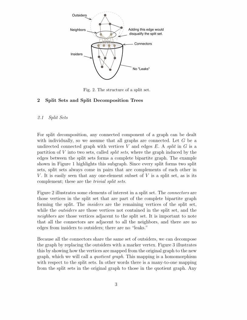
Fig. 2. The structure of a split set.

2 Split Sets and Split Decomposition Trees

2.1 Split Sets

For split decomposition, any connected component of a graph can be dealtwith individually, so we assume that all graphs are connected. Let G be aundirected connected graph with vertices V and edges E. A split in G is apartition of V into two sets, called split sets, where the graph induced by theedges between the split sets forms a complete bipartite graph. The exampleshown in Figure 1 highlights this subgraph. Since every split forms two splitsets, split sets always come in pairs that are complements of each other inV . It is easily seen that any one-element subset of V is a split set, as is itscomplement; these are the trivial split sets.

Figure 2 illustrates some elements of interest in a split set. The connectors arethose vertices in the split set that are part of the complete bipartite graphforming the split. The insiders are the remaining vertices of the split set,while the outsiders are those vertices not contained in the split set, and theneighbors are those vertices adjacent to the split set. It is important to notethat all the connectors are adjacent to all the neighbors, and there are noedges from insiders to outsiders; there are no “leaks.”

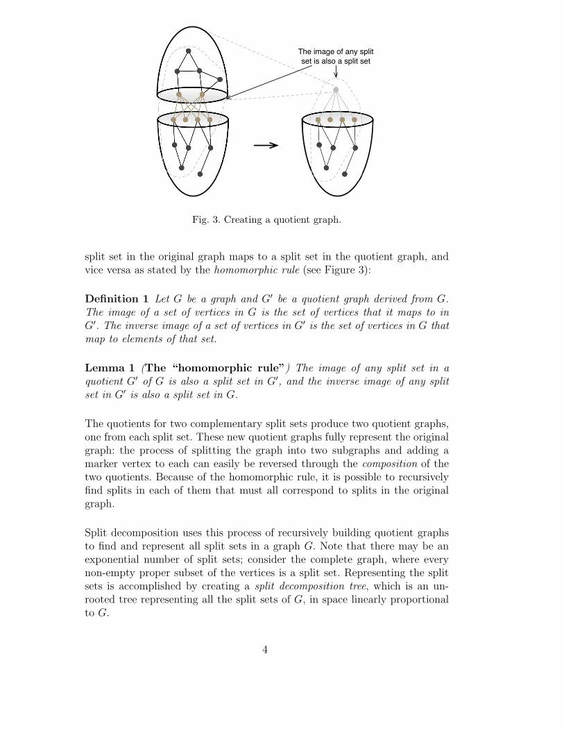
Because all the connectors share the same set of outsiders, we can decomposethe graph by replacing the outsiders with a marker vertex. Figure 3 illustratesthis by showing how the vertices are mapped from the original graph to the newgraph, which we will call a quotient graph. This mapping is a homomorphismwith respect to the split sets. In other words there is a many-to-one mappingfrom the split sets in the original graph to those in the quotient graph. Any

3

The image of any split

set is also a split set

Fig. 3. Creating a quotient graph.

split set in the original graph maps to a split set in the quotient graph, andvice versa as stated by the homomorphic rule (see Figure 3):

Definition 1 Let G be a graph and G′ be a quotient graph derived from G.The image of a set of vertices in G is the set of vertices that it maps to inG′. The inverse image of a set of vertices in G′ is the set of vertices in G thatmap to elements of that set.

Lemma 1 (The “homomorphic rule”) The image of any split set in aquotient G′ of G is also a split set in G′, and the inverse image of any splitset in G′ is also a split set in G.

The quotients for two complementary split sets produce two quotient graphs,one from each split set. These new quotient graphs fully represent the originalgraph: the process of splitting the graph into two subgraphs and adding amarker vertex to each can easily be reversed through the composition of thetwo quotients. Because of the homomorphic rule, it is possible to recursivelyfind splits in each of them that must all correspond to splits in the originalgraph.

Split decomposition uses this process of recursively building quotient graphsto find and represent all split sets in a graph G. Note that there may be anexponential number of split sets; consider the complete graph, where everynon-empty proper subset of the vertices is a split set. Representing the splitsets is accomplished by creating a split decomposition tree, which is an un-rooted tree representing all the split sets of G, in space linearly proportionalto G.

4

a

b

c

d

e f

g

hi

j

k

npqr

stu

x

w

v

y

g h

rs

t

j k

np

i

q

f

bd

ea

cuv

w

yx 5

7

31

4

2

6

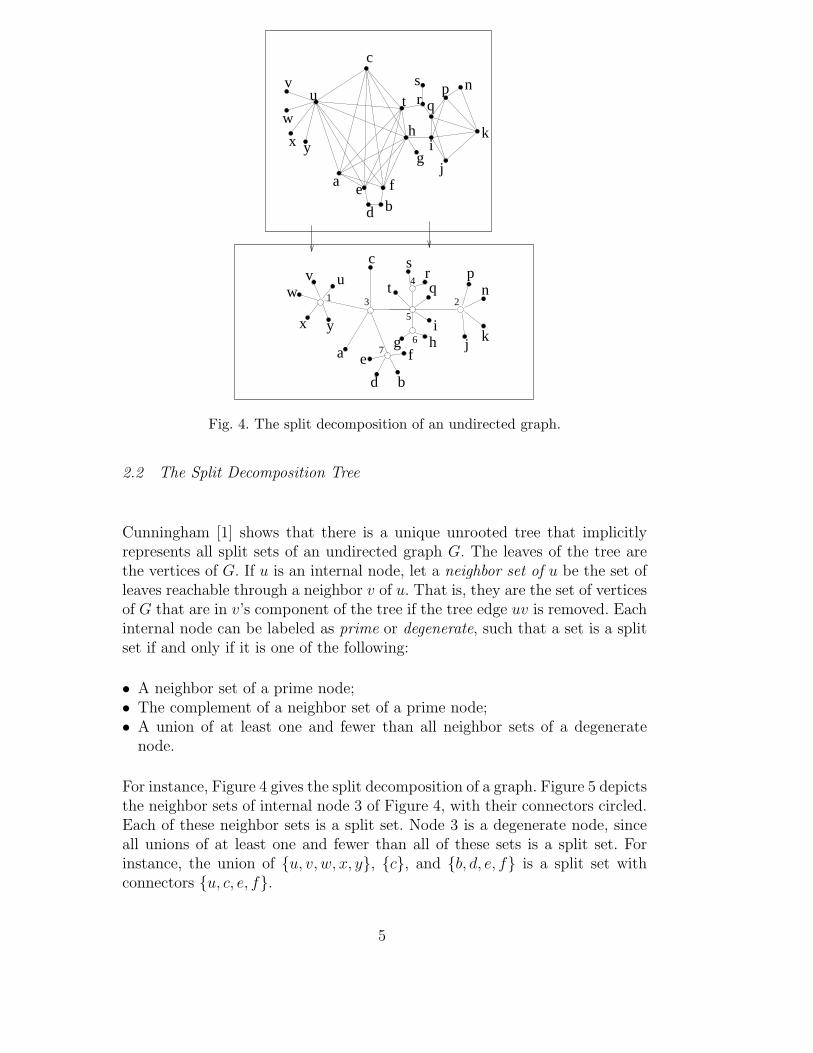
Fig. 4. The split decomposition of an undirected graph.

2.2 The Split Decomposition Tree

Cunningham [1] shows that there is a unique unrooted tree that implicitlyrepresents all split sets of an undirected graph G. The leaves of the tree arethe vertices of G. If u is an internal node, let a neighbor set of u be the set ofleaves reachable through a neighbor v of u. That is, they are the set of verticesof G that are in v’s component of the tree if the tree edge uv is removed. Eachinternal node can be labeled as prime or degenerate, such that a set is a splitset if and only if it is one of the following:

• A neighbor set of a prime node;• The complement of a neighbor set of a prime node;• A union of at least one and fewer than all neighbor sets of a degenerate

node.

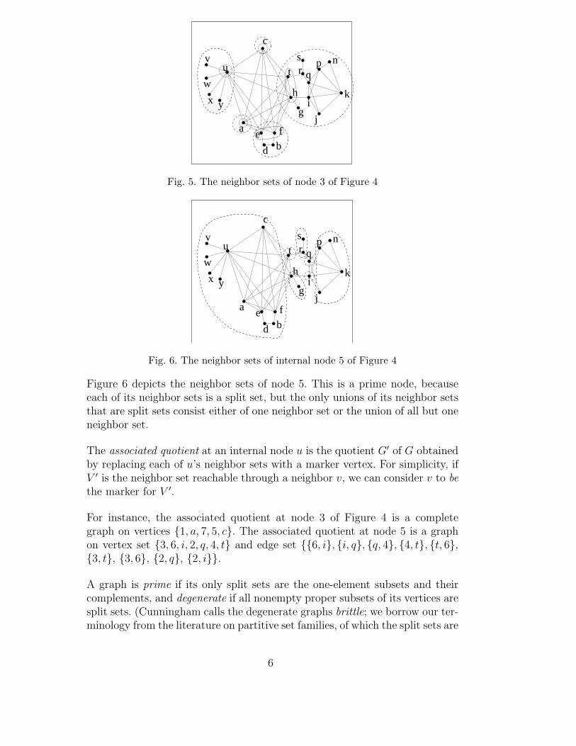
For instance, Figure 4 gives the split decomposition of a graph. Figure 5 depictsthe neighbor sets of internal node 3 of Figure 4, with their connectors circled.Each of these neighbor sets is a split set. Node 3 is a degenerate node, sinceall unions of at least one and fewer than all of these sets is a split set. Forinstance, the union of {u, v, w, x, y}, {c}, and {b, d, e, f} is a split set withconnectors {u, c, e, f}.

5

a

bd

e f

g

hi

j

k

npqr

stu

x

w

v

y

c

Fig. 5. The neighbor sets of node 3 of Figure 4

a

b

c

d

e f

g

hi

j

k

npqr

stu

x

w

v

y

Fig. 6. The neighbor sets of internal node 5 of Figure 4

Figure 6 depicts the neighbor sets of node 5. This is a prime node, becauseeach of its neighbor sets is a split set, but the only unions of its neighbor setsthat are split sets consist either of one neighbor set or the union of all but oneneighbor set.

The associated quotient at an internal node u is the quotient G′ of G obtainedby replacing each of u’s neighbor sets with a marker vertex. For simplicity, ifV ′ is the neighbor set reachable through a neighbor v, we can consider v to bethe marker for V ′.

For instance, the associated quotient at node 3 of Figure 4 is a completegraph on vertices {1, a, 7, 5, c}. The associated quotient at node 5 is a graphon vertex set {3, 6, i, 2, q, 4, t} and edge set {{6, i}, {i, q}, {q, 4}, {4, t}, {t, 6},{3, t}, {3, 6}, {2, q}, {2, i}}.

A graph is prime if its only split sets are the one-element subsets and theircomplements, and degenerate if all nonempty proper subsets of its vertices aresplit sets. (Cunningham calls the degenerate graphs brittle; we borrow our ter-minology from the literature on partitive set families, of which the split sets are

6

Complete Star

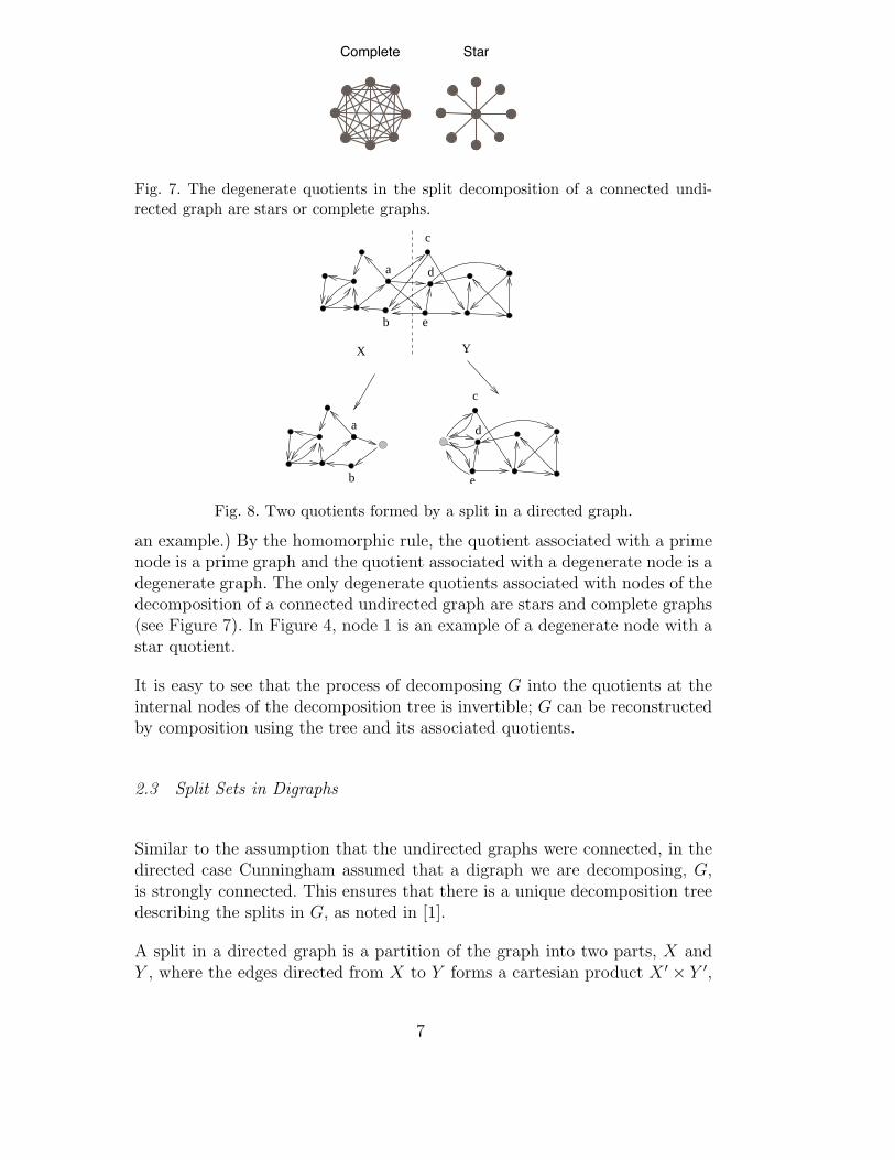
Fig. 7. The degenerate quotients in the split decomposition of a connected undi-rected graph are stars or complete graphs.

b

a

c

d

e

b

a

c

d

e

X Y

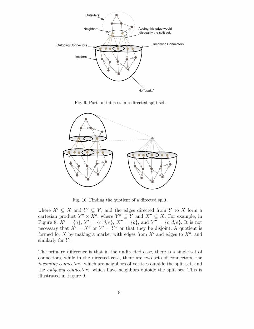
Fig. 8. Two quotients formed by a split in a directed graph.

an example.) By the homomorphic rule, the quotient associated with a primenode is a prime graph and the quotient associated with a degenerate node is adegenerate graph. The only degenerate quotients associated with nodes of thedecomposition of a connected undirected graph are stars and complete graphs(see Figure 7). In Figure 4, node 1 is an example of a degenerate node with astar quotient.

It is easy to see that the process of decomposing G into the quotients at theinternal nodes of the decomposition tree is invertible; G can be reconstructedby composition using the tree and its associated quotients.

2.3 Split Sets in Digraphs

Similar to the assumption that the undirected graphs were connected, in thedirected case Cunningham assumed that a digraph we are decomposing, G,is strongly connected. This ensures that there is a unique decomposition treedescribing the splits in G, as noted in [1].

A split in a directed graph is a partition of the graph into two parts, X andY , where the edges directed from X to Y forms a cartesian product X ′ × Y ′,

7

No "Leaks"

Insiders

Outgoing Connectors

Neighbors Adding this edge would

disqualify the split set.

Outsiders

Incoming Connectors

Fig. 9. Parts of interest in a directed split set.

Fig. 10. Finding the quotient of a directed split.

where X ′ ⊆ X and Y ′ ⊆ Y , and the edges directed from Y to X form acartesian product Y ′′ × X ′′, where Y ′′ ⊆ Y and X ′′ ⊆ X. For example, inFigure 8, X ′ = {a}, Y ′ = {c, d, e}, X ′′ = {b}, and Y ′′ = {c, d, e}. It is notnecessary that X ′ = X ′′ or Y ′ = Y ′′ or that they be disjoint. A quotient isformed for X by making a marker with edges from X ′ and edges to X ′′, andsimilarly for Y .

The primary difference is that in the undirected case, there is a single set ofconnectors, while in the directed case, there are two sets of connectors, theincoming connectors, which are neighbors of vertices outside the split set, andthe outgoing connectors, which have neighbors outside the split set. This isillustrated in Figure 9.

8

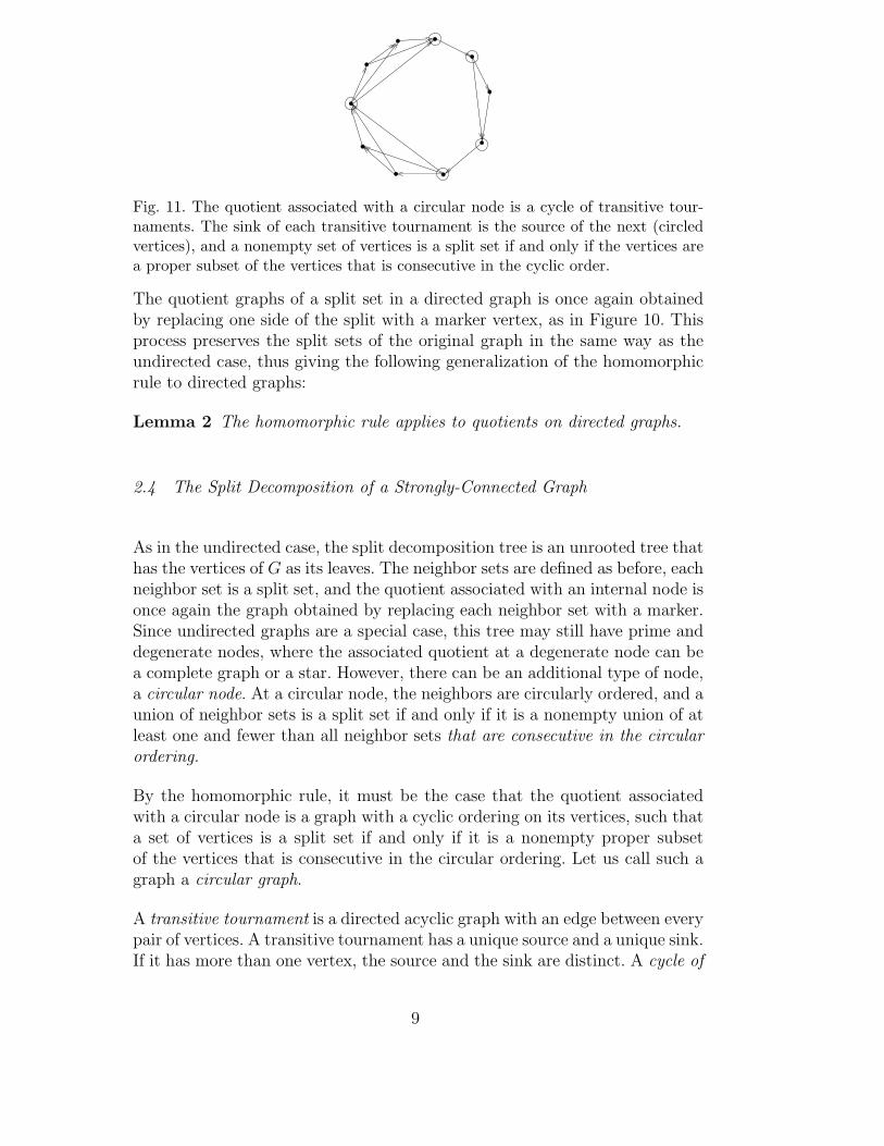
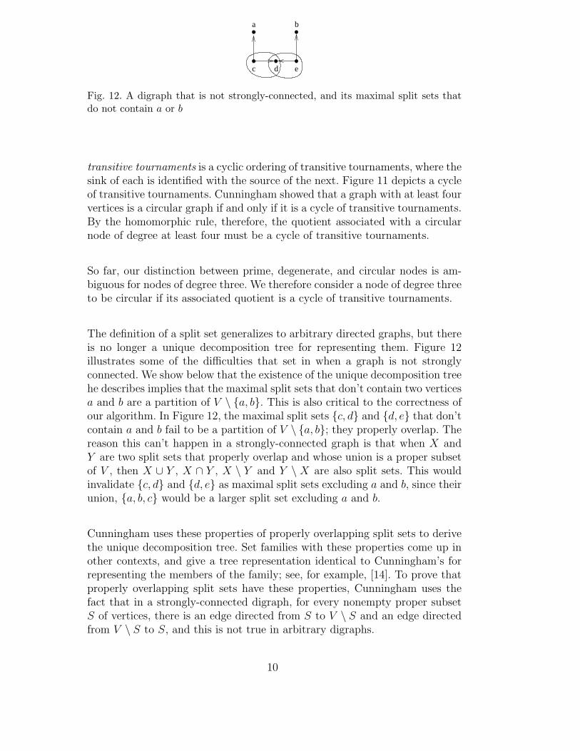
Fig. 11. The quotient associated with a circular node is a cycle of transitive tour-naments. The sink of each transitive tournament is the source of the next (circledvertices), and a nonempty set of vertices is a split set if and only if the vertices area proper subset of the vertices that is consecutive in the cyclic order.

The quotient graphs of a split set in a directed graph is once again obtainedby replacing one side of the split with a marker vertex, as in Figure 10. Thisprocess preserves the split sets of the original graph in the same way as theundirected case, thus giving the following generalization of the homomorphicrule to directed graphs:

Lemma 2 The homomorphic rule applies to quotients on directed graphs.

2.4 The Split Decomposition of a Strongly-Connected Graph

As in the undirected case, the split decomposition tree is an unrooted tree thathas the vertices of G as its leaves. The neighbor sets are defined as before, eachneighbor set is a split set, and the quotient associated with an internal node isonce again the graph obtained by replacing each neighbor set with a marker.Since undirected graphs are a special case, this tree may still have prime anddegenerate nodes, where the associated quotient at a degenerate node can bea complete graph or a star. However, there can be an additional type of node,a circular node. At a circular node, the neighbors are circularly ordered, and aunion of neighbor sets is a split set if and only if it is a nonempty union of atleast one and fewer than all neighbor sets that are consecutive in the circularordering.

By the homomorphic rule, it must be the case that the quotient associatedwith a circular node is a graph with a cyclic ordering on its vertices, such thata set of vertices is a split set if and only if it is a nonempty proper subsetof the vertices that is consecutive in the circular ordering. Let us call such agraph a circular graph.

A transitive tournament is a directed acyclic graph with an edge between everypair of vertices. A transitive tournament has a unique source and a unique sink.If it has more than one vertex, the source and the sink are distinct. A cycle of

9

b

e

a

dc

Fig. 12. A digraph that is not strongly-connected, and its maximal split sets thatdo not contain a or b

transitive tournaments is a cyclic ordering of transitive tournaments, where thesink of each is identified with the source of the next. Figure 11 depicts a cycleof transitive tournaments. Cunningham showed that a graph with at least fourvertices is a circular graph if and only if it is a cycle of transitive tournaments.By the homomorphic rule, therefore, the quotient associated with a circularnode of degree at least four must be a cycle of transitive tournaments.

So far, our distinction between prime, degenerate, and circular nodes is am-biguous for nodes of degree three. We therefore consider a node of degree threeto be circular if its associated quotient is a cycle of transitive tournaments.

The definition of a split set generalizes to arbitrary directed graphs, but thereis no longer a unique decomposition tree for representing them. Figure 12illustrates some of the difficulties that set in when a graph is not stronglyconnected. We show below that the existence of the unique decomposition treehe describes implies that the maximal split sets that don’t contain two verticesa and b are a partition of V \ {a, b}. This is also critical to the correctness ofour algorithm. In Figure 12, the maximal split sets {c, d} and {d, e} that don’tcontain a and b fail to be a partition of V \ {a, b}; they properly overlap. Thereason this can’t happen in a strongly-connected graph is that when X andY are two split sets that properly overlap and whose union is a proper subsetof V , then X ∪ Y , X ∩ Y , X \ Y and Y \ X are also split sets. This wouldinvalidate {c, d} and {d, e} as maximal split sets excluding a and b, since theirunion, {a, b, c} would be a larger split set excluding a and b.

Cunningham uses these properties of properly overlapping split sets to derivethe unique decomposition tree. Set families with these properties come up inother contexts, and give a tree representation identical to Cunningham’s forrepresenting the members of the family; see, for example, [14]. To prove thatproperly overlapping split sets have these properties, Cunningham uses thefact that in a strongly-connected digraph, for every nonempty proper subsetS of vertices, there is an edge directed from S to V \ S and an edge directedfrom V \ S to S, and this is not true in arbitrary digraphs.

10

3 Examples of Applications

A well known application of split decomposition in graph theory is the recog-nition and isomorphism testing of circle graphs [15,2]. Circle graphs are thosegraphs whose vertices are each a chord of the circle, and whose edges are thepairs of chords that intersect. Equivalently, given a set of arcs on the circle,the pairs of arcs that properly overlap is a circle graph, as two arcs properlyoverlap if and only if the chord joining one arc’s endpoints intersects the chordjoining the other’s endpoints. Any circle graph that is prime with respect tosplit decomposition has a unique chord representation, that is, the order ofendpoints of chords about the circle is uniquely constrained up to reversal oftheir order. Conversely, any split represents two sets of chords, one of whoseendpoint placements is not uniquely constrained by the other’s. The split de-composition yields a gadget, analogous to the so-called PQ tree for intervalgraphs, that represents all possible arc endpoint placements.

Parity graphs can also be recognized using split decomposition [16,9], and ithas been shown recently that split decomposition can be used when computingthe coloring of a graph [3]. A graph is perfect if and only if every prime graphin the split decomposition is perfect [17].

Distance hereditary graphs are those undirected graphs that can be built byadding pendant vertices or duplicating existing vertices [18]. An alternativecharacterization is that all induced paths between any two vertices have thesame length. A third characterization is in terms of forbidden subgraphs: theyare the class of graphs that have no gem, house, domino, or hole as an inducedsubgraphs [19]. A fourth is that they are precisely the class of undirectedgraphs whose split decompositions have no prime nodes. (Their role in splitdecomposition is analogous to that of the so-called cographs in modular de-composition.)

Split decomposition has the potential to speed up hard computations by run-ning the process on each component of the decomposed graph, and then com-bining the results to create the final answer. Finding the maximum weightedindependent set is one example of an NP-hard problem on undirected graphsthat can be optimized on graphs with non-trivial split decompositions. For abrief description of how to accomplish this see [1]. In the directed case, theexample mentioned by Cunningham is the minimum-weight dominating setfor directed graphs. The running time using this strategy is exponential in themaximum degree of a prime node, rather than exponential in the number ofvertices, providing a heuristic that only fails to be useful if the graph is prime.

11

a

b c

u

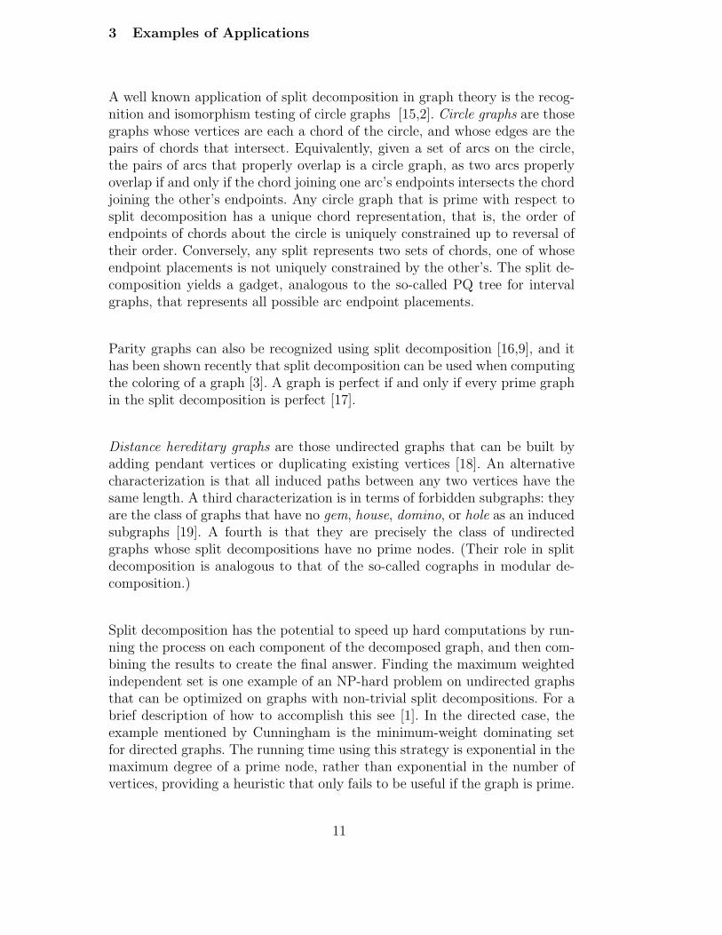
Fig. 13. The paths connecting a, b, and c cross at a node u.

4 Finding the Decomposition Tree of an Undirected Graph

To simplify the discussion, let us assume for the moment that all internalnodes of the decomposition tree are prime.

4.1 The Strategy

We have two methods at our disposal that are described below: S(a, b,G)which returns the partition of V consisting of {a}, {b}, and the maximal splitsets in G that don’t contain a or b, and L(a, b, c, G) which finds the maximalsplit set in G that doesn’t contain a or b but does contain c. We show belowthat S(a, b,G) is, in fact, a partition of V , and, because L(a, b, c, G) is themember of S(a, b,G) that contains c, it is unique. We could get L(a, b, c, G) byrunning S(a, b,G) and removing all returned sets except the one that containsc, but we use a separate procedure for efficiency reasons. Using these methodswe can show how to construct the entire split decomposition tree of G.

The first step is to pick three vertices a, b, c of G. Because they are verticesof G, they must be leaf nodes of G’s split decomposition tree. We don’t yetknow what the G’s decomposition tree looks like, but we do know that thepaths connecting a, b, and c in the tree must intersect at single internal node,which we will call u. Figure 13 shows u in relation to the nodes we have chosenin the final, still unknown, decomposition tree. Let A, B, and C denote theneighbor sets of u that contain a, b, and c, respectively.

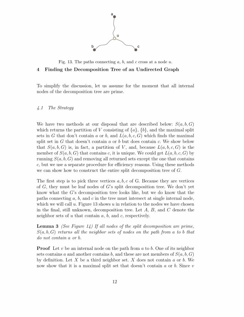
Lemma 3 (See Figure 14) If all nodes of the split decomposition are prime,S(a, b,G) returns all the neighbor sets of nodes on the path from a to b thatdo not contain a or b.

Proof Let v be an internal node on the path from a to b. One of its neighborsets contains a and another contains b, and these are not members of S(a, b,G)by definition. Let X be a third neighbor set. X does not contain a or b. Wenow show that it is a maximal split set that doesn’t contain a or b. Since v

12

a

b

u

c

A

B

Fig. 14. What we get from calling S(a, b, G).

!

"

u

c

!

"

u

c

!

"

u

c

Fig. 15. Completing the decomposition tree through recursion.

is prime, the minimal split sets that properly contain X are unions of all butone neighbor set of v, hence each of them contains at least one of a and b,which reside in different neighbor sets. ¤

Equivalently, S(a, b,G) finds all neighbor sets of u that correspond to neigh-bors that are not on the path from a to b, but are adjacent to nodes on thepath. Therefore these sets are a partition of V \ {a, b}, hence S(a, b,G) is apartition of V . By Lemma 3, A is a union of {a} and neighbor sets of thosenodes on the path from a to u in the decomposition tree that correspond toneighbors that do not lie on this path. Similarly, B is a union of {b} andneighbor sets adjacent to the path from b to u.

From S(a, b,G), we cannot tell which members of S(a, b,G) are neighbor setsof u, which are subsets of A and which are subsets of B. To find which aresubsets of A and B, it suffices to call L(b, c, a,G) and L(a, c, b, G), respectively.The remaining sets are neighbor sets of u, and, since we now know A and B,we now know all neighbor sets of u.

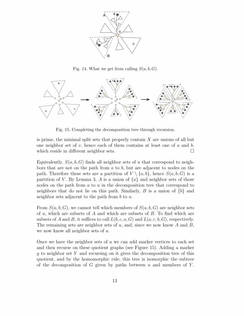
Once we have the neighbor sets of u we can add marker vertices to each setand then recurse on these quotient graphs (see Figure 15). Adding a markery to neighbor set Y and recursing on it gives the decomposition tree of thisquotient, and by the homomorphic rule, this tree is isomorphic the subtreeof the decomposition of G given by paths between u and members of Y .

13

Repeating this operation on all neighbor sets Y and identifying the markervertex therefore gives the full decomposition tree of G.

4.2 Introducing degenerate nodes

Let us now relax the assumption that u is prime. Because any nonemptyproper subset of a degenerate node’s neighbor sets is also a split set, andbecause S(a, b,G) finds maximal split sets that don’t contain a or b, if v is adegenerate node on the path from a to b in the tree, the union of all neighborsets of v, other than the ones that contain a and b, are a single member ofS(a, b,G). Lemma 3 must be modified:

Lemma 4 S(a, b,G) returns {a}, {b}, and a partition of V \{a, b} where eachpartition class consists of the neighbor sets of a prime node on the path from a

to b that do not contain a or b, or the union of all neighbor sets of a degeneratenode on the path from a to b that do not contain a or b.

Proof The characterization of neighbor sets of prime nodes is given byLemma 3. Let v be an internal degenerate node on the path from a to b.One of its neighbor sets contains a and another contains b, and these are notmembers of S(a, b,G) by definition. Let X be the union of all other neighborsets of v. Because v is degenerate, X is a split set. Because there is no largerunion of neighbor sets that excludes a and b, it is a set returned by S(a, b,G).

¤

If u is degenerate, let X be the union of neighbor sets of u other than A and B

returned by S(a, b,G). By induction, we may assume that a recursive call onthe quotient consisting of X and a marker produces the split decompositionof this graph. Let w be the marker. Making w be a neighbor of u, and doingthe same for the results of recursive calls on A and B makes u a tree nodeof degree three. If X is the union of more than one neighbor set of u in theactual decomposition of G, then this is incorrect, because u should have oneneighbor for each of these, instead of just w. We resolve this in a way thatis described by Cunningham [1]. The quotient associated with u identifiesone of its markers with w and the quotient at w identifies one of its markerswith u. This situation is detected by checking whether the composition of thequotients associated with u and w give rise to a larger degenerate quotient (acomplete graph or a star). If so, then we contract tree edge uw, and replacethe quotient at the resulting node with this composition. Since A and B areeach a single neighbor set of u and the recursive call on X produces the correcttree for X’s quotient, no other contraction is required to produce the correcttree for G.

14

Finished NeighborsUnfinished Neighbors

InternalVertices

Connectors

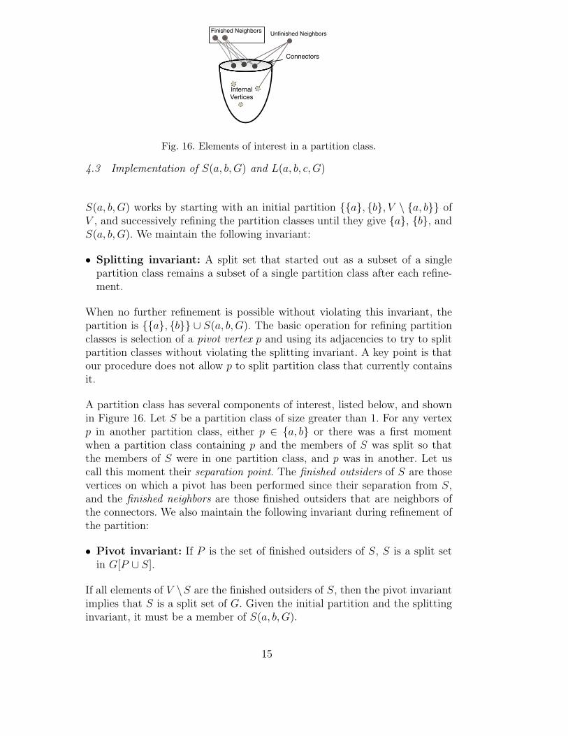
Fig. 16. Elements of interest in a partition class.

4.3 Implementation of S(a, b,G) and L(a, b, c, G)

S(a, b,G) works by starting with an initial partition {{a}, {b}, V \ {a, b}} ofV , and successively refining the partition classes until they give {a}, {b}, andS(a, b,G). We maintain the following invariant:

• Splitting invariant: A split set that started out as a subset of a singlepartition class remains a subset of a single partition class after each refine-ment.

When no further refinement is possible without violating this invariant, thepartition is {{a}, {b}} ∪ S(a, b,G). The basic operation for refining partitionclasses is selection of a pivot vertex p and using its adjacencies to try to splitpartition classes without violating the splitting invariant. A key point is thatour procedure does not allow p to split partition class that currently containsit.

A partition class has several components of interest, listed below, and shownin Figure 16. Let S be a partition class of size greater than 1. For any vertexp in another partition class, either p ∈ {a, b} or there was a first momentwhen a partition class containing p and the members of S was split so thatthe members of S were in one partition class, and p was in another. Let uscall this moment their separation point. The finished outsiders of S are thosevertices on which a pivot has been performed since their separation from S,and the finished neighbors are those finished outsiders that are neighbors ofthe connectors. We also maintain the following invariant during refinement ofthe partition:

• Pivot invariant: If P is the set of finished outsiders of S, S is a split setin G[P ∪ S].

If all elements of V \S are the finished outsiders of S, then the pivot invariantimplies that S is a split set of G. Given the initial partition and the splittinginvariant, it must be a member of S(a, b,G).

15

Finished NeighborsFinished Neighbors

Unfinished Neighbors

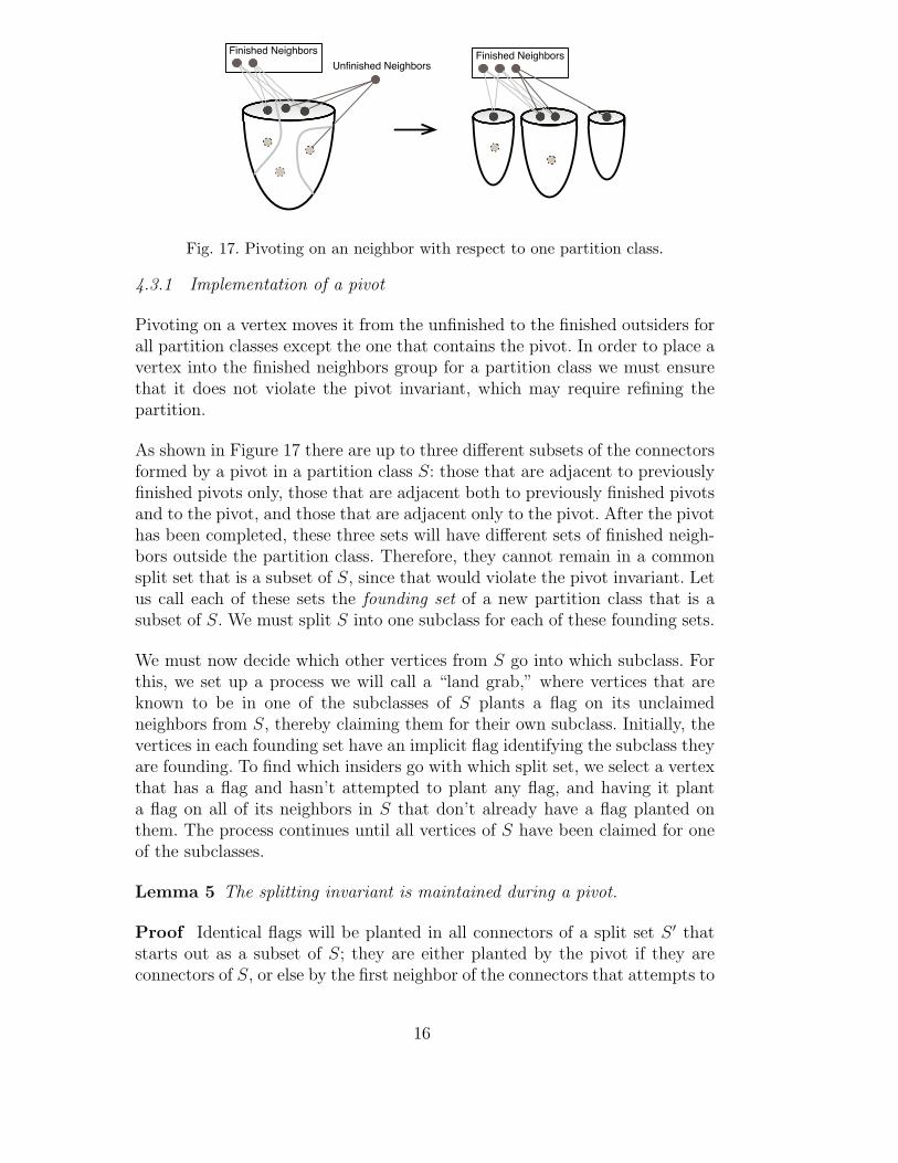
Fig. 17. Pivoting on an neighbor with respect to one partition class.

4.3.1 Implementation of a pivot

Pivoting on a vertex moves it from the unfinished to the finished outsiders forall partition classes except the one that contains the pivot. In order to place avertex into the finished neighbors group for a partition class we must ensurethat it does not violate the pivot invariant, which may require refining thepartition.

As shown in Figure 17 there are up to three different subsets of the connectorsformed by a pivot in a partition class S: those that are adjacent to previouslyfinished pivots only, those that are adjacent both to previously finished pivotsand to the pivot, and those that are adjacent only to the pivot. After the pivothas been completed, these three sets will have different sets of finished neigh-bors outside the partition class. Therefore, they cannot remain in a commonsplit set that is a subset of S, since that would violate the pivot invariant. Letus call each of these sets the founding set of a new partition class that is asubset of S. We must split S into one subclass for each of these founding sets.

We must now decide which other vertices from S go into which subclass. Forthis, we set up a process we will call a “land grab,” where vertices that areknown to be in one of the subclasses of S plants a flag on its unclaimedneighbors from S, thereby claiming them for their own subclass. Initially, thevertices in each founding set have an implicit flag identifying the subclass theyare founding. To find which insiders go with which split set, we select a vertexthat has a flag and hasn’t attempted to plant any flag, and having it planta flag on all of its neighbors in S that don’t already have a flag planted onthem. The process continues until all vertices of S have been claimed for oneof the subclasses.

Lemma 5 The splitting invariant is maintained during a pivot.

Proof Identical flags will be planted in all connectors of a split set S ′ thatstarts out as a subset of S; they are either planted by the pivot if they areconnectors of S, or else by the first neighbor of the connectors that attempts to

16

plant flags. This is because all connectors of S ′ have identical neighborhoodsoutside of S ′. Once this happens, the flags on the connectors block access toall competing land grabs, as S ′ has no leaks. At this point, all of S ′ is destinedto end up with identical flags, hence in the same partition class. ¤

Lemma 6 The pivot invariant is maintained during a pivot.

Proof Let P be the finished outsiders before the pivot that splits class S. Theconnectors of the class all have P as their neighbor set outside S before thepivot. The connectors of the new subclasses are the connectors of S that haveonly P as their finished neighbor set outside of S, P ∪ {p} as their finishedneighbor set outside of S, or {p} as their neighbor finished neighbor set outsideof S. Each of the three subclasses satisfies the pivot invariant. ¤

L(a, b, c, G) performs a subset of the operations of S(a, b,G). Since we are onlyinterested in the class S that contains c, we keep only this class instead of apartition of V \ {a, b}. Whenever this class splits, we discard the subclassesthat do not contain c.

4.4 Bounding the number and density of marker elements

Definition 2 A marker vertex is one that was inserted as a marker at anypoint during execution of the algorithm. A non-marker vertex is thereforea vertex that existed in the adjacency-list representation of the original graph.The vertex size measure of a partition class is the number of non-markervertices in the class. The edge size measure is the number of non-markervertices plus the sum of sizes of their adjacency lists.

Lemma 7 The degree of a non-marker vertex in a recursive call is nevergreater than its degree in the main call.

Proof If the vertex is a connector of the split set passed to a recursive call,it gains a marker neighbor, but this marker replaces one or more neighbors ina separate split set that got passed to a separate recursive call. It gained atmost one (marker) neighbor and lost at least one neighbor. If it is an internalnode of the split set, then all of its neighbors were also neighbors in the parentcall. In each case, its degree in a recursive call is bounded by its degree in theparent call. ¤

Note that for the correctness, there is no restriction on the choice of a and b.Therefore, we adopt the following rule:

• Suppose in a recursive call on G′ = (V ′, E ′) (which might be G), we make acall to S(a, b,G′). Inside the recursive call GA on the split set A containing

17

a, we constrain the choice of parameters to S() by calling S(a,m,GA), wherem is the new marker representing V ′ \A. Similarly, inside the recursive callGB on the split set B containing b, we constrain the choice of parameters toS() by calling S(b,m′, GB), where m′ is the new marker representing V ′ \B.The choice of parameters to S() in all other recursive calls is unconstrained.

Lemma 8 There are at most two markers in any recursive call G′, and ifthere are any, they are used as a or b in the call to S(a, b,G′).

Proof The proof is by induction on the depth of the call. Suppose that itis true for the call on G′. Then only a and b can be markers. a and b arepassed to different calls, one on GA, with added marker m, and one on GB,with added marker m′, so in GA, only a and m can be markers and they areused as parameters for the call on S() in GA, and in GB, only b and m′ canbe markers, and they are used as parameters for the call on S() in GB. ¤

Corollary 1 In a recursive call or partition class with at least three verticesthat occurs during a call to S(a, b,G) or L(a, b, c, G), let k be the sum of degreesof the vertices and let k′ be the edge size measure for the call. Then k = O(k′).

Proof By Lemma 8, at most one edge fails to be incident to a non-marker,and there is at least one non-marker. ¤

4.5 Recurring implementation tricks

4.5.1 The ripe rule

Execution of S() involves incremental refinement a partition of the vertices ofG. A recurring trick in what follows is to charge vertices and their adjacency-list elements for time spent by the algorithm. A key element of the chargingscheme is to charge at intervals that ensure that they are not charged toooften. In particular, we charge an element for O(1) time only if one of the sizemeasures of the class that currently contains it has half the same size measureof the class that contained it the last time the was charged. Whether we use thevertex size measure or the edge size measure depends on the circumstances. Akey requirement of the size measure of the class containing an element neverincreases, and can decrease if the class containing the element is split into twoclasses, in which case the element finds itself in a smaller class.

Since the size measure of a class containing an element can halve O(log m) =O(log n2) = O(log n) times, and there are O(m) vertices and adjacency-listelements, this ensures that the total charges are O(m log n). We obtain theO(m log n) bound by charging in this way all costs that are difficult to boundby a simpler method.

18

The reason for using the non-marker vertices as a measure of the size of aclass is that it satisfies the requirement that the size measure of the classcontaining a vertex never grows. A measure based on all vertices in a classfails this criterion, since marker vertices are added to classes when they becomerecursive calls, giving rise to moments when the class grows.

To make the accounting easier, whenever we charge an element in a class, wecharge all elements to the class. This maintains the invariant that all elementsof a class become eligible to be charged at the same time.

Definition 3 A partition class is ripe if the last time its members werecharged, they were in a partition class that had at least twice the size mea-sure of their current class. A vertex and its adjacency-list elements are ripe

if it is a member of a ripe partition class.

The rule can be summarized as charging only elements that are in ripe classes.The measure of the size of a partition class depends on the circumstances. Letus refer to this as the ripe rule.

Proposition 1 Whenever a partition class is split into two partition classes,at least one of the subclasses becomes ripe.

When a class S splits into two smaller classes, S1 and S2, at least one of themhas at most half the size measure of S. This is the motivation for including onlynon-marker vertices in the size measures. If marker vertices were included, theproposition could fail if S1 and S2 then have marker vertices added to themand both could have more than half the size measure of S.

Even though the non-marker vertices determine whether a class becomes ripe,it allows us to charge marker vertices and their adjacency lists in a ripe class;this presents no problem for the argument, as we show below that the numberof marker elements and their adjacency-list elements that are added in allrecursive calls is O(m), and the ripe rule ensures that each of them is chargedO(log n) times.

4.5.2 The complement trick

When we wish to perform some operation on a class S that is not ripe, forinstance, removing adjacency-list elements from it that point to vertices inother partition classes, we often find that S is the only class that is not ripe,because of Proposition 1. Since all elements in the complement of S are ripe,we can operate on S by traversing all adjacency lists of all vertices not in S,charging them according to the ripe rule. In the process we can identify alledges from elements outside of S to elements inside of S, which identifies edgesof S to elements outside of S without traversing adjacency-list elements in S

19

or charging to them. These can then be removed from S if the adjacency listsare implemented with doubly-linked lists.

The complement trick comes up in various guises in what follows. On occasion,we touch elements in a class that is not ripe; this is allowed as long as we cancharge the cost of touching them to elements in a different class that is ripe.

4.6 Data Structures

For the graph, we use a dynamic adjacency-list representation of the graph G

where each adjacency-list element is in a doubly-linked list, and where eachvertex is labeled with its current degree, and each adjacency-list element hasa pointer to the vertex whose adjacency list it resides in. In addition, if v is anelement in u’s adjacency list, then this element has a pointer to its twin edge,that is, the occurrence of u in v’s adjacency list. We do this when we splitG into induced subgraphs for the recursive calls. Clearly, we can perform theinverse of this operation in O(1) time, which we do when we insert a marker.

Proposition 2 When we remove a vertex v from the adjacency list of u, ittakes O(1) time to remove u from the adjacency list of v. It takes O(1) timeto look up the current degree of a vertex, given a pointer to it.

Definition 4 Partition Class: We use the following data structure to im-plement a partition class:

• A doubly-linked list of known connectors of the class, where each elementhas a pointer to the header of this list and the header has a pointer to thelast element of the list.

• A doubly-linked list of internal vertices in the class, where each element hasa pointer to the header of this list and the header has a pointer to the lastelement.

• A pointer from the header of each of these two lists to a class header, whichkeeps a count of its degree sum, number of vertices, number of non-markervertices, number of known connectors, and other counters as needed.

Proposition 3 Using the above data structure to implement a partition class,we get the following operations:

• Remove a connector or an internal vertex from a class, given a pointer toit in O(1) time;

• Add a known connector or an internal vertex to a class by inserting it atthe end of the appropriate doubly-linked list in O(1) time;

• Identify the class that a vertex belongs to and to determine whether it is aknown connector, given a pointer to the vertex in O(1) time;

20

• Retrieve the current vertex size measure of the class in O(1) time;• Retrieve the current edge size measure of the class in O(1) time;• Merge two instances of Partition Class in time proportional to the num-

ber of vertices in the smaller of the two, where the new set of connectorsis the union of the two old sets of connectors, and the new set of internalvertices is the union of the two old sets of internal vertices.

• Support a next-vertex iterator, which returns a vertex that next-vertexhasn’t already returned since the last time that the iterator was initialized orthe vertex was inserted to the class. It returns null if such a vertex doesn’texist. Each iteration takes O(1) time.

The next-vertex iterator is implemented with a pointer to the next un-returned element in the list of known connectors and the next unreturnedelement in the list of internal vertices. Since newly inserted elements are ap-pended to the lists, the iterator can return elements that were inserted afterthe iterator was initialized.

4.7 Preparing recursive calls

When we generate recursive calls on a set of split sets, we remove eachadjacency-list element corresponding to an edge that goes from a vertex inone recursive call to a vertex in another. We then add a marker to create thesubgraph that is passed to the recursive call. This avoids passing any extra-neous edges to a recursive call that are not part of the recursive subproblem.Let us call this the cleanup operation.

The operation serves as an illustration of an application of both the ripe ruleand the complement trick. For this operation, we use the vertex size measure(Definition 3) in applying the ripe rule.

The sets {S1, S2, . . . , Sk} passed to recursive calls are split sets. By Proposi-tion 3, we can identify the split set Si with the largest number of non-markervertices in O(k) time. We traverse all adjacency lists in each class Sj 6= Si,removing all adjacency-list elements that go to a vertex in a class other thanSj. Sj is ripe. By Proposition 3, it takes O(1) time to identify whether anadjacency-list element goes to a vertex in another class. When we remove v

from u’s adjacency list, we remove u from v’s adjacency list in O(1) time,by Proposition 2. When we have done this for all classes other than Si, Si

has no vertex v with an adjacency-list element pointing to a vertex u in anySj 6= Si, as this was removed when v was removed from u’s adjacency list.Si was cleaned up even though it may not have been ripe; this illustrates anexample of the complement trick.

21

4.8 Properties of the largest partition class when no vertex is ripe

We use the edge size measure in determining ripeness of a class when perform-ing pivots in a call to S(). We perform pivots on ripe vertices until no vertexis ripe.

Whenever we perform a pivot on a vertex p, we must traverse its adjacencylist. Whenever we find an adjacency-list element that points to a vertex q

in another class from the one that contains p, we move its twin element tothe front of q’s adjacency list. This takes O(1) time given the doubly-linkedrepresentation of the adjacency lists, the twin pointers, and pointer of eachadjacency-list element to the vertex whose list it is in. Therefore, the cost ofthis reshuffling of adjacency lists is subsumed by the other costs of the pivot.Let us call this the reshuffling operation.

Lemma 9 If all vertices outside a class S have performed a pivot since thelast time they were in the same class as members of S, then the neighborsoutside the class of occupy prefixes of the adjacency lists of connectors of S.

Proof Let c be a connector of S. When each neighbor of S performed apivot, it was moved to the front of c’s adjacency list. No other vertices aremoved forward in c’s adjacency list. Since a pivot has been performed on allneighbors of S, they occupy a prefix of c’s adjacency list. ¤

Lemma 10 Let S be a partition class with the largest edge size measure whenno vertex is ripe. A pivot has been performed on all vertices outside of S sincethe last time they were in the same class as members of S.

Proof Each vertex v outside of S is in a class with at most the size measureas S has, hence at most half the size measure of the class that most recentlycontained both v and S. Therefore, v must have become ripe since splittingfrom S, and since it is no longer ripe, a pivot has been performed on v. ¤

Corollary 2 When no vertex is ripe, a partition class S with the largest sizemeasure is a member of S(a, b,G).

Proof By Lemma 10, a pivot has been performed on all vertices outsideof S since the time they last shared a partition class with members of S.All neighbors of S are therefore known neighbors. That S is a valid split setfollows from the pivot invariant, and that it is a member of S(a, b,G) followsfrom the split invariant and the fact that it is a subset of the partition classV − {a, b} that contained it at the beginning of the call to S(a, b,G). ¤

22

4.9 Bounding the cost of finding founding sets in all calls to S()

Since each partition class has at most two markers, we use as a base case aclass with two vertices, which can be handled trivially.

To select pivots, we select a ripe class P and perform a pivot on all members ofthe class. We then label the class with a last-touched label that gives its currentsize measure, which takes O(1) time to retrieve, by Proposition 3. Recall thatnone of these pivots are allowed to split P , but they can split other partitionclasses. When a class is split by a pivot, the resulting subclasses inherit its last-touched label. By Proposition 3, for each subclass, we can retrieve its currentsize measure sum in O(1) time, and by comparing this with its last-touchedlabel, we can determine whether the class is ripe in O(1) time and insert it ina list of ripe classes if it is. Since the ripe classes are kept in a list, it takesO(1) time to find a ripe class when one is needed or else determine that noclass is ripe.

By Proposition 3, given a vertex p, it takes O(deg(p)) time to find the foundingsets in each partition class S that p has neighbors in. This is a matter ofremoving neighbors of p from the connectors and starting a founding set andremoving the neighbors of p from the internal vertices and starting a foundingset. The third founding set is what remains of the connectors of S. We createa fourth instance of Partition Class by moving the list I of internal verticesof S to it, in O(1) time. Since p is ripe when this happens, the total numberof times p can be used as a pivot is O(log n), and since the sum of degrees ofvertices at all times is O(m), the cost of finding founding sets in all calls toS() is O(m log n), by Lemma 1.

Below, we show how to bound the cost of all land grabs in all calls to S().First, let us examine the consequences of only pivoting on ripe vertices. Arisk is that this constraint might cause the partition refinement to halt beforethe partition classes are split sets. However, by Corollary 2, a class with thelargest edge size measure is a member of S(a, b,G).

We then pivot once on a connector c from this X (it doesn’t matter whichone, since they all have the same neighbors outside of X), and then remove X

from consideration. This pivot may split some more classes, generating moreripe sets, and restarting the partitioning.

To charge the cost of a restarting pivot on c, observe that only edges of c toneighbors lying outside of S are relevant to the pivot on c, since a pivot is notallowed to split the class that contains the pivot vertex. By Lemma 9, theseedges form a prefix of the adjacency list for c, so we may perform the pivotby traversing only this prefix. Because the removed class containing c nowconstitutes a recursive call, these elements are removed from the adjacency

23

list of c by the cleanup operation before a recursive call is started. We cancharge the cost of the restarting pivot to elements that are removed from c’slist, ensuring that no edge of c is charged twice during execution of the splitdecomposition algorithm.

4.10 Bounding the cost of land grabs in calls to S()

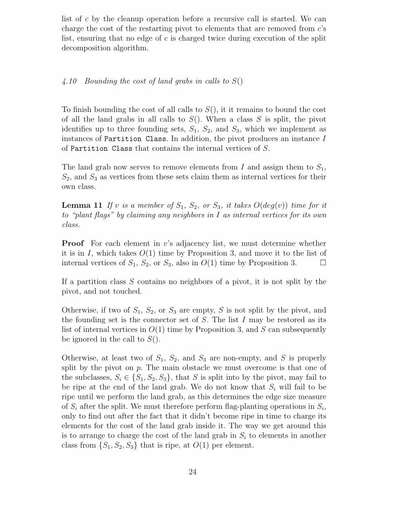
To finish bounding the cost of all calls to S(), it it remains to bound the costof all the land grabs in all calls to S(). When a class S is split, the pivotidentifies up to three founding sets, S1, S2, and S3, which we implement asinstances of Partition Class. In addition, the pivot produces an instance I

of Partition Class that contains the internal vertices of S.

The land grab now serves to remove elements from I and assign them to S1,S2, and S3 as vertices from these sets claim them as internal vertices for theirown class.

Lemma 11 If v is a member of S1, S2, or S3, it takes O(deg(v)) time for itto “plant flags” by claiming any neighbors in I as internal vertices for its ownclass.

Proof For each element in v’s adjacency list, we must determine whetherit is in I, which takes O(1) time by Proposition 3, and move it to the list ofinternal vertices of S1, S2, or S3, also in O(1) time by Proposition 3. ¤

If a partition class S contains no neighbors of a pivot, it is not split by thepivot, and not touched.

Otherwise, if two of S1, S2, or S3 are empty, S is not split by the pivot, andthe founding set is the connector set of S. The list I may be restored as itslist of internal vertices in O(1) time by Proposition 3, and S can subsequentlybe ignored in the call to S().

Otherwise, at least two of S1, S2, and S3 are non-empty, and S is properlysplit by the pivot on p. The main obstacle we must overcome is that one ofthe subclasses, Si ∈ {S1, S2, S3}, that S is split into by the pivot, may fail tobe ripe at the end of the land grab. We do not know that Si will fail to beripe until we perform the land grab, as this determines the edge size measureof Si after the split. We must therefore perform flag-planting operations in Si,only to find out after the fact that it didn’t become ripe in time to charge itselements for the cost of the land grab inside it. The way we get around thisis to arrange to charge the cost of the land grab in Si to elements in anotherclass from {S1, S2, S3} that is ripe, at O(1) per element.

24

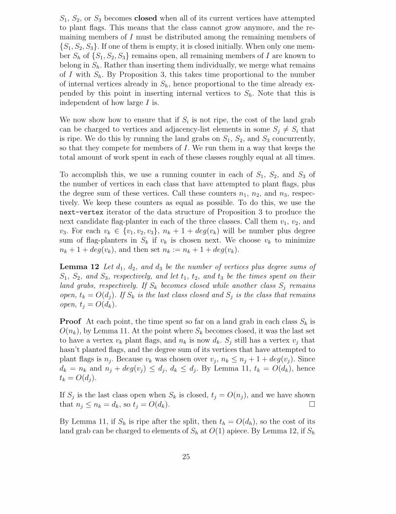
S1, S2, or S3 becomes closed when all of its current vertices have attemptedto plant flags. This means that the class cannot grow anymore, and the re-maining members of I must be distributed among the remaining members of{S1, S2, S3}. If one of them is empty, it is closed initially. When only one mem-ber Sh of {S1, S2, S3} remains open, all remaining members of I are known tobelong in Sh. Rather than inserting them individually, we merge what remainsof I with Sh. By Proposition 3, this takes time proportional to the numberof internal vertices already in Sh, hence proportional to the time already ex-pended by this point in inserting internal vertices to Sh. Note that this isindependent of how large I is.

We now show how to ensure that if Si is not ripe, the cost of the land grabcan be charged to vertices and adjacency-list elements in some Sj 6= Si thatis ripe. We do this by running the land grabs on S1, S2, and S3 concurrently,so that they compete for members of I. We run them in a way that keeps thetotal amount of work spent in each of these classes roughly equal at all times.

To accomplish this, we use a running counter in each of S1, S2, and S3 ofthe number of vertices in each class that have attempted to plant flags, plusthe degree sum of these vertices. Call these counters n1, n2, and n3, respec-tively. We keep these counters as equal as possible. To do this, we use thenext-vertex iterator of the data structure of Proposition 3 to produce thenext candidate flag-planter in each of the three classes. Call them v1, v2, andv3. For each vk ∈ {v1, v2, v3}, nk + 1 + deg(vk) will be number plus degreesum of flag-planters in Sk if vk is chosen next. We choose vk to minimizenk + 1 + deg(vk), and then set nk := nk + 1 + deg(vk).

Lemma 12 Let d1, d2, and d3 be the number of vertices plus degree sums ofS1, S2, and S3, respectively, and let t1, t2, and t3 be the times spent on theirland grabs, respectively. If Sk becomes closed while another class Sj remainsopen, tk = O(dj). If Sk is the last class closed and Sj is the class that remainsopen, tj = O(dk).

Proof At each point, the time spent so far on a land grab in each class Sk isO(nk), by Lemma 11. At the point where Sk becomes closed, it was the last setto have a vertex vk plant flags, and nk is now dk. Sj still has a vertex vj thathasn’t planted flags, and the degree sum of its vertices that have attempted toplant flags is nj. Because vk was chosen over vj, nk ≤ nj + 1 + deg(vj). Sincedk = nk and nj + deg(vj) ≤ dj, dk ≤ dj. By Lemma 11, tk = O(dk), hencetk = O(dj).

If Sj is the last class open when Sk is closed, tj = O(nj), and we have shownthat nj ≤ nk = dk, so tj = O(dk). ¤

By Lemma 11, if Sh is ripe after the split, then th = O(dh), so the cost of itsland grab can be charged to elements of Sh at O(1) apiece. By Lemma 12, if Sh

25

is a member of {S1, S2, S3} that is unripe after the split, the cost th of the landgrab in Sh can be charged to the dℓ vertices and adjacency-list elements insome other member of {S1, S2, Sk}. Since only one of the three is unripe, thischarges all costs to elements in a ripe set at O(1) apiece. Identifying whichof the other two is large enough to charge the costs to takes O(1) time byProposition 3.

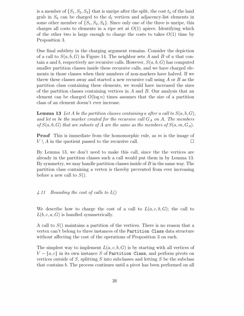
One final subtlety in the charging argument remains. Consider the depictionof a call to S(a, b,G) in Figure 14. The neighbor sets A and B of u that con-tain a and b, respectively are recursive calls. However, S(a, b,G) has computedsmaller partition classes inside these recursive calls, and we have charged ele-ments in those classes when their numbers of non-markers have halved. If wethrew these classes away and started a new recursive call using A or B as thepartition class containing these elements, we would have increased the sizesof the partition classes containing vertices in A and B. Our analysis that anelement can be charged O(log n) times assumes that the size of a partitionclass of an element doesn’t ever increase.

Lemma 13 Let A be the partition classes containing a after a call to S(a, b,G),and let m be the marker created for the recursive call GA on A. The membersof S(a, b,G) that are subsets of A are the same as the members of S(a,m,GA).

Proof This is immediate from the homomorphic rule, as m is the image ofV \ A in the quotient passed to the recursive call. ¤

By Lemma 13, we don’t need to make this call, since the the vertices arealready in the partition classes such a call would put them in by Lemma 13.By symmetry, we may handle partition classes inside of B in the same way. Thepartition class containing a vertex is thereby prevented from ever increasingbefore a new call to S().

4.11 Bounding the cost of calls to L()

We describe how to charge the cost of a call to L(a, c, b, G); the call toL(b, c, a,G) is handled symmetrically.

A call to S() maintains a partition of the vertices. There is no reason that avertex can’t belong to three instances of the Partition Class data structurewithout affecting the cost of the operations of Proposition 3 on each.

The simplest way to implement L(a, c, b, G) is by starting with all vertices ofV − {a, c} in its own instance S of Partition Class, and perform pivots onvertices outside of S, splitting S into subclasses and letting S be the subclassthat contains b. The process continues until a pivot has been performed on all

26

vertices outside of S. By the pivot and splitting invariants, S is now the max-imal split set B containing b and excluding a and c, as required. L(b, c, a,G)is implemented similarly.

Lemma 14 L(a, c, b, G) takes time proportional to the degree sum of verticesthat lie outside of the set B that it returns.

Proof A pivot on p takes O(1+deg(p)) and so does using a vertex v to plantflags. Each vertex outside of B is used once as a pivot and once to plant flags.

¤

Definition 5 A boulder is a recursive call whose size measure is more thanhalf the size measure of the parent.

Note that there can be at most one boulder. The boulder could be an elementof S(a, b,G), or it could be A or B. As in the discussion above on prepar-ing recursive calls, we can touch all elements except those that reside in theboulder, as the boulder is the only partition class that might not be ripe.

If the boulder is a member of S(a, b,G), this can be detected in O(1) timewhen it is produced in the call to S(a, b,G), by Proposition 3. To avoid havingthe call to L(a, c, b, G) touch elements internal to the boulder, we replace theboulder with a marker, yielding a quotient G′. The edges incident to the markerare generated in O(1) time apiece by Lemma 9. We remove the elements ofthe boulder from the initial partition class V \ {a, c} employed by L(a, c, b, G)by traversing elements of S(a, b,G) other than the boulder, removing themfrom this partition class, and forming a new partition class from them thatexcludes the boulder. This takes O(1) time for each element not in the boulder,thereby avoiding charging elements of the boulder. The remaining elements ofthe partition class are kept so that they can be passed into the recursive callon the boulder for use as the initial instance of Partition Class by one ofthe two calls to L() in that call. This is necessary, because assembling the classat the beginning of the call would incur charges to elements of the boulderbefore they were ripe.

Let us call this operation a boulder extraction.

We then run L(a, c, b, G′). By the homomorphic rule and the fact that theboulder is disjoint from B this call generates B, as required. By Corollary 1,the cost of generating and touching edges incident to the marker during the callto L(a, c, b, G′) can be charged to elements outside of the boulder. L(b, c, a,G)is handled similarly, and it generates a second partition class consisting of theelements of the boulder, for use by the second call to L() inside the recursivecall on the boulder.

The remaining case is when no member of S(a, b,G) is a boulder. This leaves

27

open the possibility that A or B is a boulder. Suppose B, is the boulder. If wecall L(a, c, b, G) before L(b, c, a,G), then we can charge all costs to elementsexternal to B. We can then perform a boulder extraction on B for the callto L(b′, c, a,G′), which yields A by the homomorphic rule, avoiding charges toelements internal to B.

Unfortunately, we could call L(b, c, a,G) before L(a, c, b, G), since we have noway of knowing initially which of A or B might turn out to be the boulder.Suppose B turns out to be the boulder. The call to L(b, c, a,G) would chargeelements internal to B, and we would realize this too late to undo the dam-age to the time bound. To prevent this possibility, we run L(b, c, a,G) andL(a, c, b, G) in parallel, keeping the degree sum of vertices touched so far ineach call equal to each other, using the technique we used for running landgrabs in parallel during a call to S(). That is, if the next vertex to be oper-ated on in L(b, c, a,G) has degree d1 and the next one to be operated on inL(a, c, b, G) has degree d2, add 1 + d1 to the sum of degrees of vertices oper-ated on so far in L(b, c, a,G) and add 1 + d2 to the sum of degrees of verticesoperated on so far in L(a, c, b, G), and choose the vertex that minimizes thissum to be the next operation. When L(a, c, b, G) returns the boulder, we candetect this by Proposition 3. L(a, c, b, G) has charged no elements internal tothe boulder.

If the parallel call to L(b, c, a,G) is still running, we charge the costs that ithas incurred so far to elements charged by the call to L(a, c, b, G), which hascharged at least as many elements. We undo the refinement it has performedso far so that once again PA is in its initial state, {V ′ \ b, c}. As this takesno longer than refining the classes, we may also charge its cost to elementscharged by L(a, c, b, G). We then perform a boulder extraction on B, replacingit with a marker. Let G′ be the resulting quotient. L(b, c, a,G′), which chargesto no element that is internal to the boulder, returns A, as required, by thehomomorphic rule, without charging to elements internal to the boulder.

5 Generalizing to Strongly-Connected Digraphs

Given the undirected version of the split decomposition algorithm describedabove, the directed version can be described as a set of modifications to theundirected case. Recall that the homomorphic rule still applies. The only mod-ifications that are nontrivial are the modification of the high-level strategy ofSection 4.1 to incorporate the possibility of circular nodes, and the modifi-cation to the low-level pivot operation. Once these are addressed, all otherelements of the algorithm are straightforward.

28

5.1 The Strategy

Suppose for the moment that all nodes of the decomposition tree are primeor degenerate. Since the reduction of the problem to procedures for findingS(a, b,G) and L(a, b, c, G) is based on the homomorphic rule, the reduction inthe directed case is identical to the undirected case as long as all nodes of thetree are prime or degenerate.

5.1.1 Introducing circular nodes

Let us now relax the assumption that all nodes are prime or degenerate. Letu be a circular node on the path from a to b in the decomposition tree. Be-cause any nonempty proper subset of a circular node’s neighbor sets that isconsecutive in the circular ordering of neighbor sets, the union X1 of neighborsets that lie clockwise from A and counterclockwise from B is a maximal splitset that excludes a and b, hence one member of S(a, b,G). The same is true ofthe union X2 of neighbor sets that lie counterclockwise from A and clockwisefrom B. One of X1 or X2 may be empty, in which case we ignore it.

A similar argument applies to any circular node on the path from a to b. Asin the undirected case, all members of S(a, b,G) are unions of neighbor setsof nodes on the path from a to b in the decomposition tree, and partition V \{a, b}. By induction, we may assume that recursing on the quotient consistingof X1 and a marker produces the split decomposition of this quotient. Let w1

be the neighbor of the marker. Replacing the marker with u makes w1 be aneighbor of u, and doing the same for the results of recursive calls on A, B,and X2 makes u a tree node of degree at most four (depending on whetherone of X1 and X2 is empty).

Since the quotient at u has at most four vertices, it takes O(1) time to deter-mine that it is a cycle of transitive tournaments (that is, that u is a circularnode). By induction, we may assume that the recursive calls on X1 and X2

determine whether w1 and w2 are circular nodes.

As described by Cunningham, the composition of two cycles of transitive tour-naments is a cycle of transitive tournaments, so we contract the edge uw1 andperform the composition on their quotients if they are both circular. We do thesame for uw2. This has the effect of making each neighbor set that comprisedX1 be a neighbor set of u in the final tree, and similarly for X2.

We select a and b as before. The proof of Lemma 8 goes through withoutchange; each recursive call has at most two markers. There are still at mosttwo directed edges that are not incident to non-marker vertices. Since G isstrongly-connected, Corollary 1 therefore still applies; at any point, the total

29

number of directed edges in recursive calls, counting those incident to markers,is O(m), where m is the number of directed edges of G.

5.1.2 Implementation of a pivot

We must now use two types of pivots, incoming pivots, and outgoing pivots.Below is a breakdown of how this ends up affecting the structure of a partitionclass. Since there are two types of pivots, a vertex outside a partition class S

is said to have been finished if both types of pivots have been performed on itsince the time that it was separated from S.

Of interest in a partition class S are the following:

• Known incoming connectors - These are vertices in S that have incomingedges from finished outsiders.

• Known outgoing connectors - These are vertices in S that have outgoingedges to finished outsiders.

• Finished incoming neighbors - These are outside vertices that are known tohave edges to known incoming connectors.

• Finished outgoing neighbors - These are outside vertices that are known tohave edges to known incoming connectors.

• Insiders internal to the split set - Vertices inside the S that don’t have anyedges incident finished neighbors.

Note that the outgoing and incoming connector sets may overlap.

Our incoming pivot invariant is that the known incoming connectors allhave incoming edges from the same set of finished outsiders. Our outgoing

pivot invariant is that the known outgoing connectors all have outgoingedges to the same set of finished outsiders.

Assume that both the incoming and outgoing pivot invariants apply before anoutgoing pivot on a vertex p. The goal of an outgoing pivot on a vertex p isto turn p into a known incoming neighbor of all partition classes in which p

has neighbors, partitioning the classes in order to satisfy both the incomingand outgoing pivot invariant while observing the split invariant. The goal ofan incoming pivot on p is defined symmetrically.

The way we accomplish this for an outgoing pivot is to perform the pivotexactly as we did in the directed case, performing the same operations on theadjacency lists as we did before. For an outgoing pivot, we do this on thetranspose of the graph, where the adjacency list of each vertex v is its list ofvertices that have directed edges to v. We show that performing pivots in thisway preserves both the incoming and outgoing pivot invariants.

30

Recall that in the undirected case, when no vertex is ripe in a call to S(),all vertices outside of a largest class S have been used as pivots since the lasttime they were in a common class with S. This will still be true for our versionof the algorithm for strongly-connected digraphs. As before, this ensures thatall connectors and neighbors are known, except that now we say that allincoming and outgoing connectors and all incoming and outgoing neighborsare known. Because the incoming and outgoing pivot invariants apply, S mustbe a split set. Because the split invariant applies, S must be a largest splitset that started in a single partition class, hence a member of S(a, b,G) orL(a, b, c, G).

5.2 Data Structures

For the graph, we use a dynamic adjacency-list representation of the graph G

where each vertex v carries two doubly-linked adjacency lists: one that givesthe neighbors of v (the out-neighbors) and one that gives the vertices that havev as a neighbor (the in-neighbors). Given an adjacency-list representation ofthe graph where only the lists of out-neighbors are given, it takes O(m) timeto find the in-neighbors of each vertex, by radix sorting a copy of the list ofedges using destination vertex as the primary key and vertex of origin as thesecondary key, and then cutting the list into segments that share the samedestination vertex. If (u, v) is an edge, then the occurrence of v in u’s out-neighbor list carries a pointer to the occurrence of u in v’s in-neighbor list, andthe occurrence of u in v’s in-neighbor list carries a pointer to the occurrenceof v in u’s out-neighbor list. When v is removed from u’s out-neighbor list,this allows u to be removed from v’s in-neighbor list, or vice versa, in O(1)time.

The degree of a vertex v, denoted deg(v), is the number of in-neighbors andout-neighbors, and each vertex is labeled with its current degree. Let deg+(v)denote the out-degree, that is, the number of out-neighbors, and deg−(v) de-note the in-degree, that is, the number of in-neighbors.

Definition 6 The edge size measure of a partition class in a directed graphis the number of non-marker vertices plus the sum of their degrees.

The structure of partition classes is similar to those in the undirected case.However, in the directed case, there are two types of connectors, the outgoingconnectors and the incoming connectors. There are also internal vertices thatare not connectors. We modify the Partition Class structure of Definition 4by giving it three lists, one for the outgoing connectors, one for the incomingones, and one for the internal vertices. As before, these lists are doubly-linked,the elements have pointers to the list headers, the list headers have pointers

31

to a class header, which keeps track which keeps a count of its vertex sizemeasure, edge size measure, and other counters as needed.

Proposition 4 Using the above data structure to implement a partition class,it takes O(1) time to perform any of the following operations:

• Remove an outgoing connector, an incoming connector, or an internal vertexfrom a class, given a pointer to it;

• Add an outgoing connector, an incoming connector, or an internal vertexto a class by inserting it at the end of the appropriate doubly-linked list;

• Identify the class that a vertex belongs to and to determine whether it is aknown connector, given a pointer to the vertex;

• Retrieve any of the counters stored in the class header;• Merge two instances of Partition Class in time proportional to the num-

ber of vertices in the smaller of the two, where the new set of incomingconnectors is the union of the two old sets of incoming connectors, the newset of outgoing connectors is the union of the old ones, and the new set ofinternal vertices is the union of the old ones.

• Support a next-vertex iterator, which returns a vertex that next-vertexhasn’t already returned since the last time that the iterator was initialized orthe vertex was inserted to the class. It returns null if such a vertex doesn’texist.

5.3 Preparing recursive calls

As before, when we generate recursive calls on a set of split sets, we removeedges that go from elements in one recursive call to another, and we use thevertex size measure in determining when a class is ripe.

Lemma 7 goes through with trivial changes:

Lemma 15 The in-degree and out-degree of a non-marker vertex in a recur-sive call is never greater than these degrees in the main call.

Proof If the vertex is an incoming connector of the split set passed to arecursive call, it gains a marker neighbor, but this marker replaces one or morein-neighbors in a separate split set that got passed to a separate recursive call.It gained at most one (marker) neighbor and lost at least one neighbor. Bya symmetric argument, if it is an outgoing connector, its out-degree does notincrease. If it is an internal node of the split set, then all of its in-neighborswere also in-neighbors in the parent call and all of its out-neighbors were alsoout-neighbors in the parent call. In each case, its degree in a recursive call isbounded by its degree in the parent call. ¤

32

The sets {S1, S2, . . . , Sk} passed to recursive calls are still split sets. By Propo-sition 4, we can identify the split set Si with the largest number of non-markervertices in O(k) time. We traverse all out-neighbor and in-neighbor lists ineach class Sj 6= Si, removing all elements residing in a class Sk other thanSj, and, while we’re at it, we remove the twin adjacency elements in Sk. Thistakes O(1) time for each adjacency-list element in all sets other than Si, butremoves all adjacency-list elements in Si that reside in classes other than Si.Since each class other than Si has half the non-marker vertices that the parentcall has, each adjacency-list is traversed O(log n) times in all calls to cleanupoperations.

5.4 Implementation of a pivot

We describe how an outgoing pivot on vertex v and partition class S works;an incoming pivot is defined symmetrically. It works just as in an undirectedgraph, where the outgoing adjacency lists assume the role of the undirectedadjacency lists and the known incoming connectors assume the role of theknown connectors. With this change, the founding sets are defined as before:those known incoming connectors that have the pivot as an in-neighbor thoseknown incoming connectors that don’t have the pivot as an in-neighbor, andthose that are in neither of these categories, but have the pivot as an in-neighbor.

Once again, a pivot is not allowed to split the partition class that contains it.By Proposition 4, it takes O(deg+(p)) time to obtain instances S1, S2, S3 ofthe Partition Class data structure for representing these the founding setsfor each partition class S, as well as an instance of the Partition Class datastructure representing the set I = S \ (S1 ∪ S2 ∪ S3).

As before, in traversing the adjacency list of p, whenever we find an adjacency-list element that points to a vertex in another class from the one that containsp, we move it to the front of the adjacency list for p and we move its twin ele-ment to the front of its adjacency list. This takes O(1) time given the doubly-linked representation of the adjacency lists, the twin pointers, and pointer ofeach adjacency-list element to the vertex whose list it is in. Therefore, thecost of this reshuffling of adjacency lists is subsumed by the other costs of thepivot. Let us again call this the reshuffling operation.

Lemma 16 If pivots have been performed on each vertex outside of a class S

since it was last in the same class as members of S, all in-neighbors occupya prefix of each incoming connector’s in-neighbor list, and all out-neighborsoccupy a prefix of each outgoing connector’s out-neighbor list.

The proof is a trivial variant of the proof of Lemma 9.

33

An outgoing flag planting is the operation of allowing a vertex v of S1, S2, andS3 to move its out-neighbors in I to the partition class in {S1, S2, S3} thatcontains v.

An outgoing pivot on class S once again consists of finding the incomingfounding sets {S1, S2, S3}, then letting these sets grow by planting outgoingflags until all vertices in the three sets have planted outgoing flags.

Lemma 17 If the incoming and outgoing pivot invariants are observed by S

before an outgoing pivot, then the partition classes vertices of S1, S2, and S3

have planted outgoing flags, these three partition classes observe the incomingand outgoing pivot invariants.

Proof Let P be the finished incoming outsiders before the outgoing pivotthat splits class S. The connectors of the class all have P as their in-neighborsoutside S before the pivot. The incoming connectors of the new subclasses arethe connectors of S that have only P , P∪{p}, or {p} as their finished incomingneighbors outside of S. They thus satisfy the incoming pivot invariant. Theoutgoing connectors of the new classes are subsets of the outgoing connectors ofS. If Q is the set of known out-neighbors of S, it remains the set of known out-neighbors of each of {S1, S2, S3}. All out-connectors of each of the classes haveQ as their known out-neighbors, so they satisfy the outgoing pivot invariant.

¤

Lemma 18 After all vertices of S1, S2, and S3 have planted outgoing flags,the partition of S observes the splitting invariants.

Proof Identical flags will be planted in all incoming connectors of a split set S ′

that starts out as a subset of S; they are either planted by the pivot if they areconnectors of S, or else by the first neighbor of the connectors that attempts toplant flags. This is because all connectors of S ′ have identical neighborhoodsoutside of S ′. Once this happens, the flags on the connectors block access toS ′ to all competing land grabs, as S ′ has no incoming edges other than thoseinto its incoming connectors. Because G is strongly-connected, there are pathsfrom every incoming connector of S ′ to all other members of S ′. The land grabwill expand out along these paths, giving all of S ′ identical flags, hence S ′ willreside in a single partition class. ¤

An incoming pivot is defined symmetrically, and symmetric versions of Lem-mas 17 and 18 apply. It follows from Lemma 17 and its symmetric version thatwhen all outside in-neighbors and out-neighbors of a class are known, it sat-isfies the requirements of a split set. It therefore follows from Lemma 18 andits symmetric version that when all outside in-neighbors and out-neighbors ofa class are known, it is a member of S(a, b,G).

34

5.5 Bounding the cost of finding founding sets in all calls to S()

As before, we perform a pivot on a vertex p only if the edge-size measure ofits class has halved since the last time it was used as a pivot.

When we perform a incoming or outgoing pivot on p, we perform both in-coming and outgoing pivots on all vertices in its class. By Proposition 4, ittakes O(deg+(p)) to find the founding sets in all partition classes that con-tain neighbors of p and do not contain p. We use last-touched labels on theclasses, just as before, to identify classes of vertices that are ripe. Since atall times the number of edges in all recursive calls is O(m) and the eligibilityrequirement ensures that each time O(1) time is spent on the adjacency-listelements of a vertex, the number of non-marker vertices in its class halves, ittakes O(m log n) time to find founding sets in all calls to S() made during thecourse of the algorithm.

The risk in observing this eligibility requirement is once again that there maybe no eligible vertices at some point before S(a, b,G) has been computed.However, once again, at this point, a class S with a largest number of non-marker vertices must be a valid split set.

Performing one pivot on an outgoing c1 connector of S and one on an incomingconnector c2 of S restarts the partitioning, and S can be removed, as it is aknown member of S(a, b,G). As before, Lemma 16 ensures that the adjacency-list elements of each class S that point to vertices outside of S are prefixes ofthe outgoing adjacency list of c1 and the incoming adjacency list of c2. Theseare the only edges that are relevant to performing the partition, and since S

is a split set, it constitutes a recursive call, and these edges are discarded fromthese adjacency lists before the recursive calls start, by the cleanup operation.Therefore, no edge of c1 or c2 is charged twice for a restarting pivot duringexecution of the algorithm.

5.6 Bounding the cost of land grabs in all calls to S()

By Proposition 4, Lemma 11 generalizes to the directed case, except thatplanting the flags takes time proportional to the out-degree of the flag planterif the pivot is an outgoing pivot and time proportional to the in-degree if thepivot is an ingoing pivot.

We discuss the cost of bounding the cost of outgoing pivots; the bound isobtained in a symmetric way for incoming pivots. As before, class S is splitinto instances S1, S2, S3 and I of the Partition Class data type by anincoming neighbor p, where S1, S2, and S3 are the founding sets, and I is the

35

set of vertices that will be claimed by the land grab. S1, S2, and S3 are theincoming connectors of the new subclasses that will form. I is formed in O(1)time by moving the lists of outgoing connectors and internal vertices of S toa new instance of the Partition Class data type.

The flag-planting operation is similar to the one in the undirected case, exceptthat the vertices in I are classified as outgoing connectors or internal vertices,and they retain this status when moved to S1, S2, and S3. In addition, if theflag planter is an incoming connector that is also an outgoing connector, itmoves its occurrence in I as an outgoing connector to the list of outgoingconnectors of its own class. This adds O(1) to the cost of flag-planting, whichis subsumed by other costs.

A class becomes closed when all vertices have been used as outgoing flagplanters. When all but one class, Si, is closed, the remaining vertices in I aremoved to the open class by transferring the two lists of outgoing connectors andinternal vertices to Si, and then appending the current outgoing connectorsand internal vertices to these lists, just as before. The cost of moving the listsis O(1) and the cost of appending is ones that are already there is subsumedby the cost incurred before all but Si was closed.

As before, we let a class become ripe each time the number of vertices plus thedegree sum halves. We let n1, n2, and n3 be the number of flag-planters usedso far, plus the degrees of these flag planters in S1, S2, and S3, respectively. Weuse an iterator from each class to produce the three candidates, v1, v2, and v3

to be the next flag-planters, and choose vk that minimizes nk + 1 + deg+(vk).

For the generalization of Lemma 12, we let d1, d2, and d3 be the number ofvertices plus degree sums of the vertices. The times t1, t2, t3 spent at anypoint are O(d1), O(d2), and O(d3) as before, as the number of vertices plusout-degrees in a class is bounded by the number of vertices plus degrees. Withthese observations, the proof of Lemma 12 goes through unchanged. Therefore,if one of S1, S2, and S3 is not ripe after the land grab, we can charge the timespent on the land grab to elements of one of the other classes, which is ripe,by the fact that Corollary 1 applies also in the directed case.

We again consider the depiction of a call to S(a, b,G) in Figure 14. The neigh-bor sets A and B of u that contain a and b, respectively, are recursive calls.However, S(a, b,G) has computed smaller partition classes inside these recur-sive calls, and we have charged elements in those classes when their numbers ofnon-markers have halved. Because it is based on the homomorphic rule, whichis general to strongly-connected digraphs, Lemma 13 continues to apply.

As before, if G′ is GA in the parent call, then we use the call S(a,m,GA).By Lemma 13, we don’t need to make this call, since the vertices are alreadyin the partition classes such a call would put them in by Lemma 13. By

36

Lemma 8, there are at most two markers to choose from in selecting a andb. By symmetry, we may handle partition classes inside of B in the sameway. The partition class containing a vertex is thereby prevented from everincreasing before a new call to S().

5.7 Bounding the cost of calls to L()

As before, we implement L(a, c, b, G) as the subset of operations of S(a, b,G)that lay claim to vertices in the set that contains b. The argument is the sameas the one before, except that we perform both an outgoing and incomingpivot on a vertex after it is known not to be in the class containing b that theoperation is going to be returned. Instead of being used once as a pivot andonce as a flag-planter, each vertex is used twice for each of these operation:once as an outgoing pivot and once as an outgoing flag planter, and once asan incoming pivot and once as an incoming flag planter. We have establishedthat each outgoing pivot takes O(1) time for each element in its outgoingadjacency list and each flag-planter takes O(1) time for each element in itsoutgoing adjacency list. The same is true for incoming adjacency-list elementson incoming pivots and incoming flag planters. Lemma 14 therefore applieswithout change.

Because the splitting and pivot invariants are maintained on the class con-taining b, the algorithm halts when we have the maximal split set containingb and excluding a and c, as required.

To avoid charging elements internal to a boulder, we run L(a, c, b, G) andL(b, c, a,G) in parallel, as before, keeping the work equal in both calls bychoosing from the next vertex in each call to be operated on and choosing theone that will minimize the amount of work for its call after the operation. Wecalculate this by 1 plus the out-degree to the work so far for the call if the nextoperation is an outward pivot or outward flag planting, and 1 plus the in-degreeif the next operation is an inward pivot or inward flag planting. If L(a, c, b, G)returns a boulder, it will again halt in time to extract the boulder in the callto L(b, c, a,G), and to charge the cost of incurred by L(b, c, a,G) touchingelements internal to the boulder to operations performed in L(a, c, b, G), asbefore.

6 Acknowledgments

We would like to acknowledge Haim Kaplan for helpful discussions and feed-back on this work.

37

References

[1] W. H. Cunningham. Decomposition of directed graphs. SIAM J. Algebraic

Discrete Methods, 3:214–228, 1982.

[2] C.P. Gabor, K.J. Supowit, and W.-L. Hsu. Recognizing circle graphs inpolynomial time. Journal of the ACM, 36:435–473, 1989.

[3] M. Rao. Solving some NP-complete problems using split decomposition.Discrete Applied Mathematics, 2007.

[4] R. H. Mohring and F. J. Radermacher. Substitution decomposition for discretestructures and connections with combinatorial optimization. Annals of Discrete

Mathematics, 19:257–356, 1984.

[5] R. H. Mohring. Algorithmic aspects of the substitution decomposition inoptimization over relations, set systems and boolean functions. Annals of

Operations Research, 4:195–225, 1985.

[6] A. Bouchet. Digraph decompositions and eulerian systems. SIAM Journal on

Algebraic and Discrete Methods, 8, 1987.

[7] J. Spinrad. Prime testing for the split decomposition of a graph. SIAM Journal

on Discrete Mathematics, 2:590–599, 1989.

[8] T.H. Ma and J. Spinrad. An O(n2) algorithm for undirected splitdecomposition. Journal of Algorithms, 16:145–160, 1994.

[9] E. Dahlhaus. Parallel algorithms for hierarchical clustering, and applicationsto split decomposition and parity graph recognition. Journal of Algorithms,36:205–240, 2000.

[10] J. P. Spinrad. Two Dimensional Partial Orders. PhD thesis, PrincetonUniversity, 1982.

[11] J. P. Spinrad and J. Valdes. Recognition and isomorphism of two-dimensional partial orders. In Proceedings of the 10th Colloquium on Automata,

Languages, and Programming, Lecture Notes in Computer Science, pages 676–686. Springer-Verlag, Berlin, 1983.

[12] J. P. Spinrad. On comparability and permutation graphs. Siam J. Comput.,14:658–670, 1985.

[13] J. P. Spinrad. Graph partitioning. unpublished manuscript, 1985.

[14] W.L. Hsu and R.M. McConnell. PC trees and circular-ones arrangements.Theoretical Computer Science, 296:59–74, 2003.

[15] A. Bouchet. Reducing prime graphs and recognizing circle graphs.Combinatorica, 7:243–254, 1987.

[16] S. Cicerone and di Stefano G. On the extension of bipartite to parity graphs.Discrete Applied Mathematics, 95:181–195, 1999.

38

[17] G. Cornuejols and W.H. Cunningham. Compositions for perfect graphs.Discrete Math., 55:245–254, 1985.

[18] H.J. Bandelt and H.M. Mulder. Distance-hereditary graphs. Journal of

Combinatorial Theory Series B, 41:182–208, 1986.

[19] P. L. Hammer and F. Maffray. Completely separable graphs. Discrete Applied

Mathematics, 27:85–99, 1990.

39