Embed Size (px)
Citation preview
A SunCam online continuing education course
WHAT EVERY ENGINEER SHOULD KNOW ABOUT ENGINEERING STATISTICS I
by
O. Geoffrey Okogbaa, Ph.D., PE
WHAT EVERY ENGINEER SHOULD KNOW ABOUT ENGINEERING STATISTICS I
A SunCam online continuing education course
www.SunCam.com Copyright 2017 O. Geoffrey Okogbaa, PE Page 2 of 50
TableofContentsIntroduction: The Role of Statistics and Probability in Engineering Design ................................................. 5
1.1 Probability ..................................................................................................................................... 5
1.2 Statistics ........................................................................................................................................ 5
1.3 Relationship Between Probability and Statistics .......................................................................... 5
Data Handling and Data Storage ................................................................................................................... 6
2.1 Data Analytics and ‘Big Data’ ........................................................................................................ 7
Descriptive Measures of Data ....................................................................................................................... 7
3.1 Central Tendency‐‐Mean, Median, Mode, and Mid‐Range .......................................................... 7
3.1.1 Special Case of the Equality of the Mean, Median and Mode .............................................. 9
3.1.2 Significance of Sample Statistics as Estimators of the Population Parameters .................... 9
3.1.3 The Sample Mean as the Best Estimator of the Population Mean ..................................... 10
3.2 Dispersion –Variance, Standard Deviation, Range, Interquartile Range .................................... 10
3.2.1 The Range ............................................................................................................................ 10
3.2.2 The Inter‐quartile range ...................................................................................................... 11
3.2.3 The Standard Deviation ....................................................................................................... 12
Data (Graphical) Displays ............................................................................................................................ 12
4.1 Quantitative versus Qualitative Data .......................................................................................... 12
4.2 Quantitative Data Graphs ........................................................................................................... 13
4.3 Qualitative Data Graphs .............................................................................................................. 15
Early Development of the Concept of Uncertainties and Randomness ..................................................... 17
5.1 Uncertainty and Probability Methods ........................................................................................ 18
5.1.1 Parameter uncertainty ........................................................................................................ 18
5.1.2 Data uncertainty ................................................................................................................. 18
5.1.3 Operational Uncertainties ................................................................................................... 18
Definitions ................................................................................................................................................... 18
6.1 Experiment .................................................................................................................................. 18
6.2 Sample space (S) ......................................................................................................................... 18
6.3 Outcome ..................................................................................................................................... 19
6.4 Multiple Outcomes ..................................................................................................................... 19
6.5 Events .......................................................................................................................................... 19
WHAT EVERY ENGINEER SHOULD KNOW ABOUT ENGINEERING STATISTICS I
A SunCam online continuing education course
www.SunCam.com Copyright 2017 O. Geoffrey Okogbaa, PE Page 3 of 50
6.6 Definition of A Random variable ................................................................................................. 20
Definitions of Probability ............................................................................................................................ 21
7.1 Classical Definition of Probability ............................................................................................... 21
7.2 Relative Frequency Definition/Approach ................................................................................... 21
7.3 Modern Definition/Approach ..................................................................................................... 21
7.4 Axioms (or Laws) of Probability—Addition, Multiplication, Inverse ........................................... 22
7.5 Venn Diagram Representation of the Axioms ............................................................................ 22
7.6 Mutually Exclusive Events ........................................................................................................... 24
7.7 Non‐Mutually Exclusive Events ................................................................................................... 25
7.8 Multiplication Law (Dependent Law) .......................................................................................... 25
7.9 Multiplication Law (Independent Law) ....................................................................................... 25
Counting Techniques .................................................................................................................................. 26
8.1 Multiplication or the m x n Rule ................................................................................................. 26
8.2 Permutation ................................................................................................................................ 26
8.3 Combination ................................................................................................................................ 27
8.4 General Enumeration .................................................................................................................. 28
8.5 The Tree Diagram Approach ....................................................................................................... 28
Probability Distributions ............................................................................................................................. 31
9.1 Random Variables ....................................................................................................................... 32
9.2 Domain and Range of a Random Variable .................................................................................. 32
9.3 Rules or Equations for Mapping/Assignment ............................................................................. 33
Discrete Random variables ......................................................................................................................... 34
10.1 Distribution Functions and Density Functions for Discrete Random Variables .......................... 35
10.2 Common Discrete Probability Distributions ............................................................................... 35
10.2.1 Binomial Distribution .......................................................................................................... 35
10.2.2 Negative Binomial (The Random variable is the number of trials) ..................................... 37
10.2.3 Geometric Distribution ....................................................................................................... 38
10.2.4 Hypergeometric Distribution .............................................................................................. 40
10.2.5 The Poisson Distribution or the Poisson Process ................................................................ 41
Continuous Random Variables .................................................................................................................... 43
11.1 Common Continuous Distributions ............................................................................................. 44
WHAT EVERY ENGINEER SHOULD KNOW ABOUT ENGINEERING STATISTICS I
A SunCam online continuing education course
www.SunCam.com Copyright 2017 O. Geoffrey Okogbaa, PE Page 4 of 50
11.1.1 The Normal Distribution ..................................................................................................... 44
11.1.2 Properties of the Standard Normal Distribution ................................................................. 45
11.1.3 Exponential Distribution ..................................................................................................... 47
11.1.4 The Uniform Distribution .................................................................................................... 47
Conclusion ................................................................................................................................................... 49
REFERENCES ................................................................................................................................................ 50
WHAT EVERY ENGINEER SHOULD KNOW ABOUT ENGINEERING STATISTICS I
A SunCam online continuing education course
www.SunCam.com Copyright 2017 O. Geoffrey Okogbaa, PE Page 5 of 50
Introduction:TheRoleofStatisticsandProbabilityinEngineeringDesign1.1 Probability
The concept of probability was developed to describe the property of an experimental situation in which it is impossible to tell what outcome to expect from any one experiment but yet in a series of trials (experiments), the proportion yielding a particular outcome seems fairly stable. Probability theory provides a formal basis for quantifying risk or uncertainty in engineering designs. According to Ang and Tang (1975), the role of probability methods in engineering design can be broadly categorized as – a) The modeling of engineering problems and evaluation of systems performance under conditions of uncertainty; b) Systemic development of design criteria, explicitly taking into account the significance of uncertainty, and c). The logical framework for risk assessment and risk benefit trade-off analysis relative to decision making. 1.2 Statistics
Statistics is the art and science of gathering data and making inference from such data. Statistical techniques are useful for describing and understanding variability. By variability, we mean that successive observations of the outcome from a system or phenomenon do not produce exactly the same results. Statistics gives us a framework for describing this variability and for learning about the potential sources of variability.
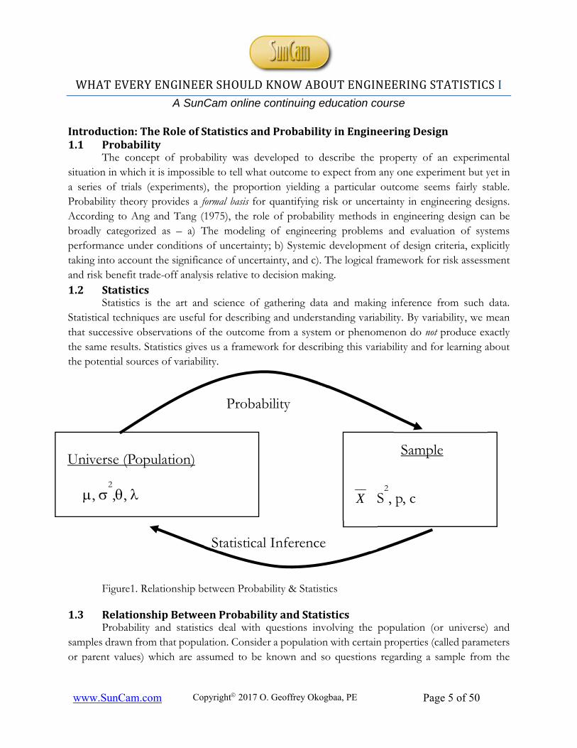
Figure1. Relationship between Probability & Statistics
1.3 RelationshipBetweenProbabilityandStatisticsProbability and statistics deal with questions involving the population (or universe) and
samples drawn from that population. Consider a population with certain properties (called parameters or parent values) which are assumed to be known and so questions regarding a sample from the
Probability
Statistical Inference
Universe (Population) Sample
, 2,, S
2, p, c X
WHAT EVERY ENGINEER SHOULD KNOW ABOUT ENGINEERING STATISTICS I
A SunCam online continuing education course
www.SunCam.com Copyright 2017 O. Geoffrey Okogbaa, PE Page 6 of 50
population or universe are posed and then answered. The problem is that because of the nature of the population, the values of the parameters are unknown but assumed and it is only by collecting samples from the population via random experiments that we can truly know the properties of a population or have an idea about the values of the parameters. For example, the probability of getting a head in a toss of a coin is assumed to be ½ and a way to verify this is through an experiment involving infinite number of trials.
Probability deals with the population with its parameters (parent values) while statistics deal with the sample and its statistic (values computed from the sample used as true representation of the population or universe parameters). Thus, while probability and statistics both deal with questions involving populations and samples, they do so in an “inverse manner” as shown in figure 1. From the point of view of the population, information about the sample can be obtained by probability analyses. On the other hand, given some sample statistics, one can use those values to make inference about the nature of the population parameters. Statistics really is about statistical inference, namely,
trying to infer whether the sample statistic (such as sample mean 𝑋 versus the population mean or
the sample standard deviation S2 versus the population variance 2 ) can reasonably be assumed to be good estimates of the parameters of the parent population. Thus, probability projects information from the population to the sample via deductive reasoning, while Statistics tend to project information from the sample to the population via inductive reasoning DataHandlingandDataStorage Data handling is one of the major activities that engage the time of engineers and scientists in general but more so engineers. Engineering activities and processes generate considerable data that have been gathered in different contexts and situations for the purpose of understanding the behaviors and patterns of the underlying distribution so that reasonable assumptions and hence engineering decisions, which are the real motive the data have been generated and gathered in the first place, can be made. In its complete form, data handling involves data collection, data recording and data presentation. Properly organized and displayed data make it easy to understand and hence interpret the data for engineering decisions. Thus, there is universal agreement among engineers that data handling is perhaps one of the most important activities of any engineer.
More recently, new developments and growth in information technology (the internet in particular) and instrumentation have resulted in the generation of massive amounts of data. Consequently, engineers and scientists are inundated with unusual amount of data, most of that generated unwittingly. New storage platforms of such unimaginable sizes have been developed over the past few years. We have gone from Kilobytes, and Megabytes just a few decades ago to now Gigabytes and Terabytes. By way of perspective, a computer Bit is the smallest unit of data that a computer uses. It can be used to represent two states of information, such as go, no-go. On a higher scale than the Bit is the
WHAT EVERY ENGINEER SHOULD KNOW ABOUT ENGINEERING STATISTICS I
A SunCam online continuing education course
www.SunCam.com Copyright 2017 O. Geoffrey Okogbaa, PE Page 7 of 50
Byte. A Byte is equal to 8 Bits. A Byte can represent 256 states of information, for example, numbers or a combination of numbers and letters. Kilobyte is yet on a higher scale than Byte. A Kilobyte is approximately 1,000 Bytes. A Megabyte is approximately 1,000 Kilobytes. A Gigabyte is approximately 1,000 Megabytes. A Gigabyte is now a common term used to refer to computer disk space or drive storage. A 500 Gigabyte hard drive computer seems to be the basic standard these days. 1 Gigabyte of data is almost twice the amount of data that a CD-ROM can hold. A Terabyte is approximately one trillion bytes, or 1,000 Gigabytes. One and two Terabyte drives are the normal specs for many new computers. As an example, a Terabyte could hold close to 1,000 copies of the Encyclopedia Britannica. It is estimated that 85,899,345 pages of Word documents would fill one Terabyte [Source: The Information Umbrella, Musings on Applied Information Management, 2014] 2.1 DataAnalyticsand‘BigData’
Thus there is now a new area of concern and study commonly referred as "Big Data." and an accompanying new methodology of data Analytics and data mining. Big data is used to describe data sets that are so large or complex that traditional data processing applications are inadequate to deal with them. Some of the challenges to Big Data handling include analysis, capture, search, sharing, storage, transfer, visualization, querying, updating and privacy.
Analytics is the discovery, interpretation, and communication of meaningful patterns in data. Data analytics have become an important tool in most engineering disciplines and are especially valuable in areas rich with recorded data. Data analytics combines basic theories and applications in statistics, computer programming and operations research to quantify performance and hence to support engineering decision making. DescriptiveMeasuresofData
For any given data, the goal is to extract some information or some of summary statistic about the data in terms of its central location and its variability. The natural tendency is to try and locate the center of the data and to know where the data is anchored. Another common measure is the dispersion or variability in the data. In other words, the measure of dispersion gives an idea about the type of variability inherent in the data. The central tendency represents a single value that attempts to describe a set of data by identifying the central position within that set of data. As such, measures of central tendency are sometimes called measures of central location and are often referred to as summary statistics. The measures of dispersion focus on different measures of variability.
3.1 CentralTendency‐‐Mean,Median,Mode,andMid‐Range
The Mean, Mode, Median and the Mid-Range are used as measures of the Central Tendency of a data set.
Mean The arithmetic means or the Mean is one statistic that describes the central tendency of a dataset and is typically denoted as 𝑋 . The population mean is denoted as .
The general formula for the sample mean is given as:
WHAT EVERY ENGINEER SHOULD KNOW ABOUT ENGINEERING STATISTICS I
A SunCam online continuing education course
www.SunCam.com Copyright 2017 O. Geoffrey Okogbaa, PE Page 8 of 50
sampleselforf
XfX
samplessmallforn
X
n
XXXXXX
i
ii
n
ii
n
arg
... 14321
Where fi is the frequency (or the number of occurrences) associated with the ith data point. Median
The Median refers to the ‘middle’ value when the data is arranged in increasing or decreasing
order. Thus, the Median is computed from ranked data and is denoted as 𝑋 (referred to as X curly) and the corresponding population value is denoted as 𝜇. For a set of values X1, X2, …..Xn, the Median is computed as shown depending on whether the sample size n is even or odd.
For n odd, The Median value is denoted as 𝑋2
1nposition
For n even, The Median 𝑋 is given by the average of the values of 2
nand
1
2
n position.
Mode The Mode of a set of observations is the observation in the data that occurs most often. Not every set of numbers has a mode. If no numbers repeat {3,5,6,9,12,8} then there is no mode. Sometimes we might have more than one mode. For example, for the set {1, 4, 4, 6, 8, 9, 9}, the modes are 4 and 9. As another example, the mode of the sample [1, 3, 4,5, 5, 6, 6, 7, 7, 7, 11, 11, 16] is 7. Given the list of data [4, 4, 2, 9, 9] the mode is not unique - the dataset may be said to be bimodal, while a set with more than two modes may be described as multimodal.
Mid-Range The Mid-Range defined [(XL+XS)/2] can also be considered as a central tendency, where XL and XS refer to the largest and smallest number in the dataset respectively. Regardless of which is used, the Central tendency is typically a point estimate of the data.
Numerical Examples for Central Tendency Set of numbers: {2, 5, 7, 8, 12, 13, 16} Mean={2+5+7+8+12+13+16}/7 Mean=63/7 Mean=9 Median={2,5,7,8,12,13,16} =8 Mode: There is no mode (No number occurs more than once) Midrange=2+16/2=9.
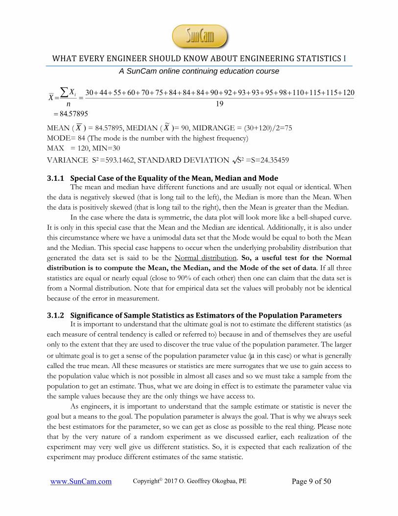
Given the set of 19 data points: 30,44,55,60,70,75,84,84,84, 90,92,93,93,95,98,110,115,115,120
WHAT EVERY ENGINEER SHOULD KNOW ABOUT ENGINEERING STATISTICS I
A SunCam online continuing education course
www.SunCam.com Copyright 2017 O. Geoffrey Okogbaa, PE Page 9 of 50
57895.8419
120115115110989593939290848484757060554430
n
XX i
MEAN ( X ) = 84.57895, MEDIAN ( X~
)= 90, MIDRANGE = (30+120)/2=75 MODE= 84 (The mode is the number with the highest frequency) MAX = 120, MIN=30
VARIANCE S2 =593.1462, STANDARD DEVIATION √S2 =S=24.35459
3.1.1 SpecialCaseoftheEqualityoftheMean,MedianandModeThe mean and median have different functions and are usually not equal or identical. When
the data is negatively skewed (that is long tail to the left), the Median is more than the Mean. When the data is positively skewed (that is long tail to the right), then the Mean is greater than the Median.
In the case where the data is symmetric, the data plot will look more like a bell-shaped curve. It is only in this special case that the Mean and the Median are identical. Additionally, it is also under this circumstance where we have a unimodal data set that the Mode would be equal to both the Mean and the Median. This special case happens to occur when the underlying probability distribution that generated the data set is said to be the Normal distribution. So, a useful test for the Normal distribution is to compute the Mean, the Median, and the Mode of the set of data. If all three statistics are equal or nearly equal (close to 90% of each other) then one can claim that the data set is from a Normal distribution. Note that for empirical data set the values will probably not be identical because of the error in measurement.
3.1.2 SignificanceofSampleStatisticsasEstimatorsofthePopulationParameters It is important to understand that the ultimate goal is not to estimate the different statistics (as each measure of central tendency is called or referred to) because in and of themselves they are useful only to the extent that they are used to discover the true value of the population parameter. The larger
or ultimate goal is to get a sense of the population parameter value ( in this case) or what is generally called the true mean. All these measures or statistics are mere surrogates that we use to gain access to the population value which is not possible in almost all cases and so we must take a sample from the population to get an estimate. Thus, what we are doing in effect is to estimate the parameter value via the sample values because they are the only things we have access to. As engineers, it is important to understand that the sample estimate or statistic is never the goal but a means to the goal. The population parameter is always the goal. That is why we always seek the best estimators for the parameter, so we can get as close as possible to the real thing. Please note that by the very nature of a random experiment as we discussed earlier, each realization of the experiment may very well give us different statistics. So, it is expected that each realization of the experiment may produce different estimates of the same statistic.
WHAT EVERY ENGINEER SHOULD KNOW ABOUT ENGINEERING STATISTICS I
A SunCam online continuing education course
www.SunCam.com Copyright 2017 O. Geoffrey Okogbaa, PE Page 10 of 50
3.1.3 TheSampleMeanastheBestEstimatorofthePopulationMean As indicated earlier, the mean is prone to the effects of outliers since it is simply the arithmetic average with no weighting involved. This means that other measure of the central tendency may be preferable. The median as a measure of central tendency for example is resistant to the effect of outliers. However, while this may be the case, it has been shown that in most situations the sample Mean tends to be a more stable estimator of the population mean. So, what we need more than anything in order to determine the most preferable estimator is the properties of unbiasedness and efficiency. So, a statistic that is both unbiased and efficient is the one that we must use to represent or estimate the parameter value. So, in the case of the central tendency while the other estimators are unbiased, the sample mean is most efficient of the group of estimators and so it is commonly
used as the estimator of the population mean (). 3.2 Dispersion–Variance,StandardDeviation,Range,InterquartileRange The measure of central tendency gives us an idea about where the data is located or anchored. However, while that information is useful, it is incomplete because as we noted earlier different samples from the population will likely give us different estimates of the central tendency. While we could have the same estimates for the Mean and Median for different samples, realistically the spread or dispersion for the different data set could be significant and hence cannot be ignored. Thus, it is important that we not only look at the central tendency but equally important, we must also look at the dispersion or the variability to a get a true sense of what the data is about. Again, it is important to realize that because of the random nature of an experiment, there is inherent variability and so it is important that we understand and estimate that variability in order to be able to get a true estimate of the population parameter. Thus, the central tendency estimates alone do not tell us the complete story and we must of necessity get a measure of the variability or dispersion to get an accurate picture of the data. The known measures of dispersion or variability are; the Variance, Standard Deviation, Range, Inter-quartile Range.
3.2.1 TheRange The sample range is the simplest measure of variability but only based on two values. It is simply the difference between the smallest value XS and XL for a given data set (. i.e., XS - XL). Because of variability, each sample from the population will have different range values. The range is a good measure of variability when the sample size is small, less than 5 and greater than or equal to 2. A good rule of thumb is to use the range as an estimator of variability if the sample size is less than 5, and to use standard deviation if the sample size is 5 or more. As we will see later, in the computation of the standard deviation, the numerator or divisor is (n-1), so the standard deviation is not a suitable estimator of variability for small sample sizes especially for sample sizes that are 2 or less. Of course, if the sample size is one (n=1), we will not be talking about variability because practically we cannot
WHAT EVERY ENGINEER SHOULD KNOW ABOUT ENGINEERING STATISTICS I
A SunCam online continuing education course
www.SunCam.com Copyright 2017 O. Geoffrey Okogbaa, PE Page 11 of 50
measure it. Of course, for very large samples, the sample variance or the square of the sample standard deviation is the most unbiased and efficient estimator of the population variance.
3.2.2 TheInter‐quartilerangeBefore discussing the inter-quartile range, it is important to we identify what quartiles are and
how they are computed to guide our discussion. The quartile is the name given to segments of the data when they are divided into fourths. The reason is that it is easy to look at such segments to see where and how the data is located
• 1st Quartile (Q1) = 25th percentile • 2nd Quartile (Q2)= 50th percentile= The Median • 3rd Quartile (Q3) = 75th percentile
The 100pth percentile for a sample set is a value such that at least 100p% of the observations in the data set are below this value and (100(1-p)% are at or above this value.
position
nQposition
nQposition
nQ
4
13,
2
1,
4
1321
Interpolations are often needed when the quartiles are not integers. For example, if n is odd, then there is no interpolation needed. However, if n is even, then for Q1 the
value will be between 4
nand
1
4
n position. For Q2 the value will be between
2
nand
1
2
n
position and for Q3 the value will be between 4
3nand
1
4
3n position. For n odd, The Median
value is 𝑋 𝑄 and corresponds to the value of the 2
1n position
For n even, The Median 𝑋 is given by the average of the values of the 2
nand
1
2
n positions
The Inter-quartile range is a measure that indicates the extent to which the central 50% of values within the dataset are dispersed. It is based upon, and related to, the median. As indicated the data can be further divided into quarters by identifying the upper and lower quartiles. The lower quartile is one-quarter of the way along a ranked or ordered dataset whereas the upper quartile or 3rd quartile is found three-quarters from the top of the dataset or one-quarter of the way from the bottom. Therefore, the upper quartile lies half way between the median and the highest value in the dataset whilst the lower quartile lies halfway between the median and the lowest value in the dataset. The inter-quartile range is the difference between the 3rd and 1st quartiles that is (Q3-Q1). Like the range however, the inter-quartile range is a measure of dispersion that is based upon only two values from the dataset.
WHAT EVERY ENGINEER SHOULD KNOW ABOUT ENGINEERING STATISTICS I
A SunCam online continuing education course
www.SunCam.com Copyright 2017 O. Geoffrey Okogbaa, PE Page 12 of 50
3.2.3 TheStandardDeviation Statistically, the standard deviation is a more powerful measure of dispersion because unlike the range and the inter-quartile range, it takes into account every value in the dataset. The square of the sample standard deviation, also known as the sample variance, is an unbiased estimator of the population variance. Please note that the sample standard deviation is NOT an unbiased estimator of the population variance, but the sample variance is.
)1(
,1
)(
22
2
2
2
nn
XXnSisformnalcomputatioThe
meansampleXwheren
XXSVariancesampleThe
ii
i
Data(Graphical)Displays The purpose of data display is to convey the data to the viewers in pictorial form that is easily understood. Data displays in the form of a graph are much more visually appealing than a table or list. A graph should be able to stand alone, without the original data. It is easier for most people to comprehend the meaning of data presented graphically than data presented numerically in the form of tables. This is especially the case for those with limited background and knowledge of engineering and statistics. More specifically, data is displayed graphically to
To describe the data set
To analyze the data set (Distribution of data set)
To summarize a data set
To discover a trend or pattern in a situation over a period of time As an important aside, several statistical packages have been created as standalone packages or as part of a main software package and are used to construct graphical displays of data. MINITAB and MATLAB are two packages that are very familiar to engineers. Also, SAS and SPSS are major packages that are universally used. Microsoft EXCEL also has graphing capability and has been found to be very useful and sufficient for this type of analyses as it contains most of the statistical tables needed for the common distributions. As a result, we will not spend a lot of time on graphing techniques or on table lookup for probabilities resulting from common distributions. 4.1 QuantitativeversusQualitativeDataData comes to us in two different forms, namely, qualitative and quantitative. a) Quantitative data is numerical and acquired through counting or measuring. There are a variety of ways that quantitative data arise in statistics. Each of the following is an example of quantitative data:
The size of steel beam ion a construction site
The dimensions of different electronic boards
The values of homes in a neighborhood
WHAT EVERY ENGINEER SHOULD KNOW ABOUT ENGINEERING STATISTICS I
A SunCam online continuing education course
www.SunCam.com Copyright 2017 O. Geoffrey Okogbaa, PE Page 13 of 50
The lifetime of a batch of a certain electronic component. b). Qualitative data sets are data sets that are not numerical. They are typically in categories separated by traits are attributes such as physical traits, gender, colors or anything that does not have a number associated to it. Qualitative data is sometimes referred to as categorical data. Qualitative data sets do not contain numbers that we can perform mathematics upon. 4.2 QuantitativeDataGraphsThe three most commonly used graphs for quantitative data include: 1. The histogram. 2. The frequency polygon. 3. The Cumulative Frequency Graph, or the Ogive 4.2.1 Histograms
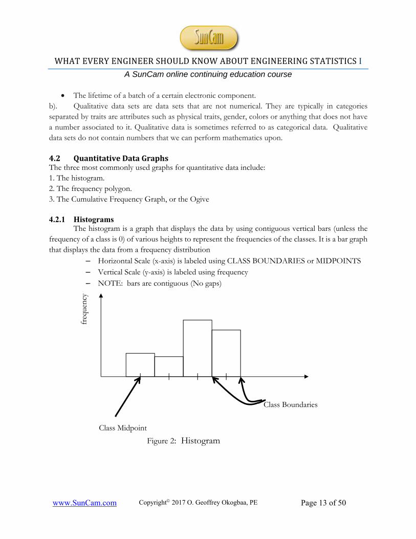
The histogram is a graph that displays the data by using contiguous vertical bars (unless the frequency of a class is 0) of various heights to represent the frequencies of the classes. It is a bar graph that displays the data from a frequency distribution
– Horizontal Scale (x-axis) is labeled using CLASS BOUNDARIES or MIDPOINTS – Vertical Scale (y-axis) is labeled using frequency – NOTE: bars are contiguous (No gaps)
Figure 2: Histogram
freq
uenc
y
Class Boundaries
Class Midpoint
WHAT EVERY ENGINEER SHOULD KNOW ABOUT ENGINEERING STATISTICS I
A SunCam online continuing education course
www.SunCam.com Copyright 2017 O. Geoffrey Okogbaa, PE Page 14 of 50
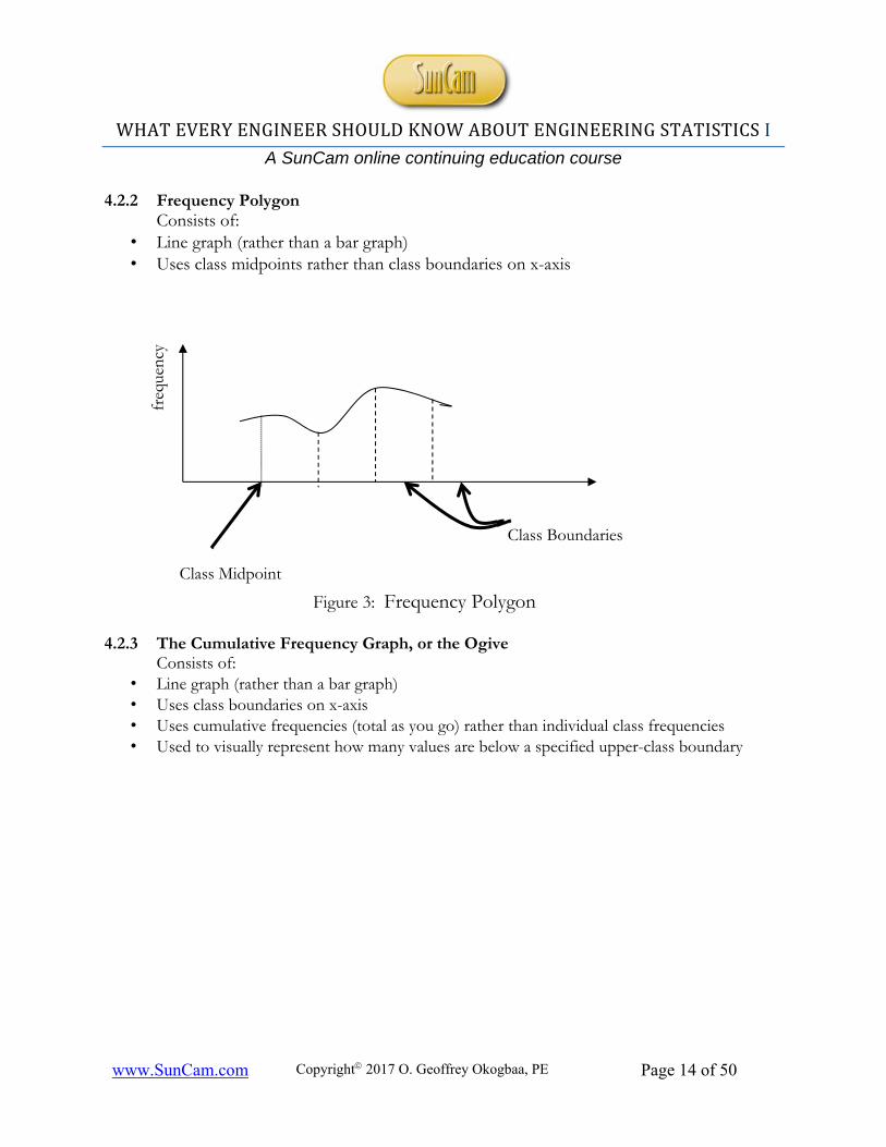
4.2.2 Frequency Polygon Consists of:
• Line graph (rather than a bar graph) • Uses class midpoints rather than class boundaries on x-axis
Figure 3: Frequency Polygon
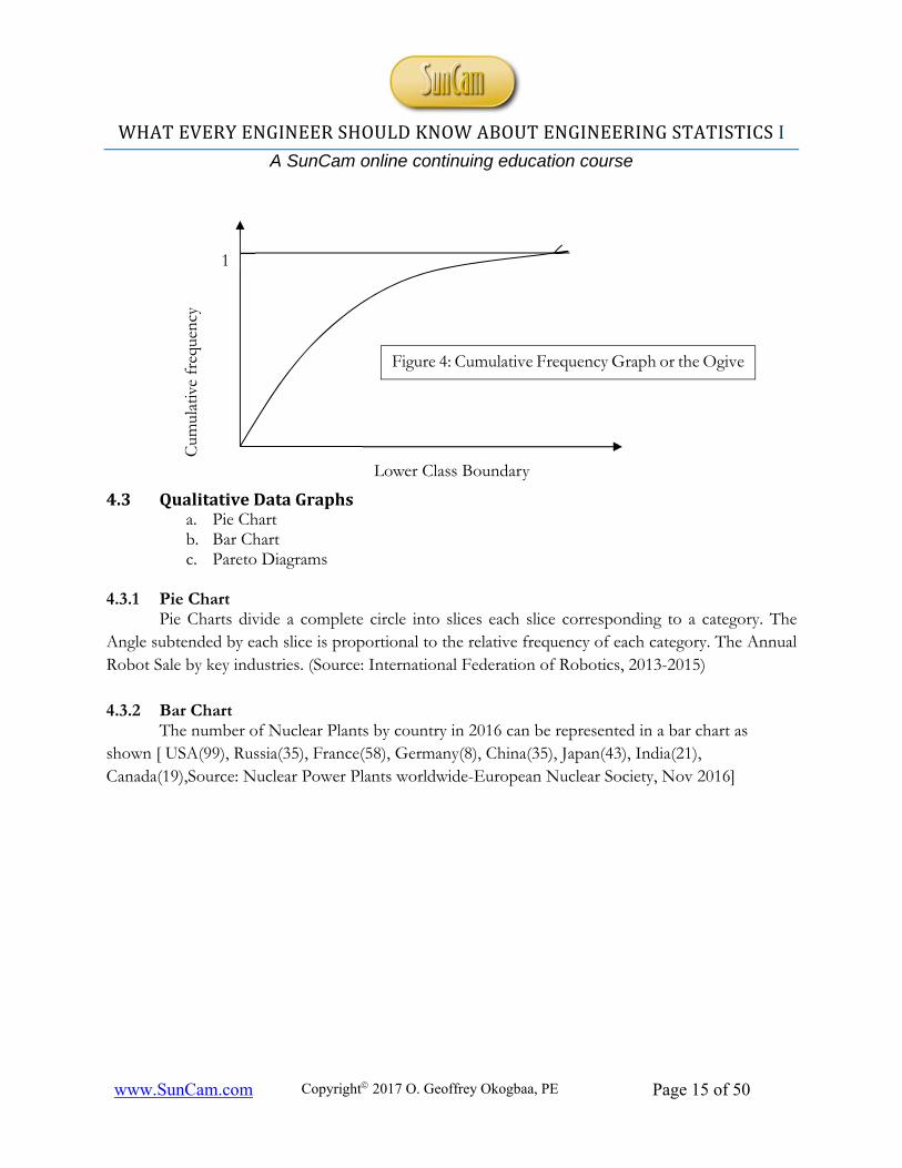
4.2.3 The Cumulative Frequency Graph, or the Ogive Consists of:
• Line graph (rather than a bar graph) • Uses class boundaries on x-axis • Uses cumulative frequencies (total as you go) rather than individual class frequencies • Used to visually represent how many values are below a specified upper-class boundary
freq
uenc
y
Class Boundaries
Class Midpoint
WHAT EVERY ENGINEER SHOULD KNOW ABOUT ENGINEERING STATISTICS I
A SunCam online continuing education course
www.SunCam.com Copyright 2017 O. Geoffrey Okogbaa, PE Page 15 of 50
4.3 QualitativeDataGraphs
a. Pie Chart b. Bar Chart c. Pareto Diagrams
4.3.1 Pie Chart
Pie Charts divide a complete circle into slices each slice corresponding to a category. The Angle subtended by each slice is proportional to the relative frequency of each category. The Annual Robot Sale by key industries. (Source: International Federation of Robotics, 2013-2015) 4.3.2 Bar Chart
The number of Nuclear Plants by country in 2016 can be represented in a bar chart as shown [ USA(99), Russia(35), France(58), Germany(8), China(35), Japan(43), India(21), Canada(19),Source: Nuclear Power Plants worldwide-European Nuclear Society, Nov 2016]
Cum
ulat
ive
freq
uenc
y
Lower Class Boundary
1
Figure 4: Cumulative Frequency Graph or the Ogive

WHAT EVERY ENGINEER SHOULD KNOW ABOUT ENGINEERING STATISTICS I
A SunCam online continuing education course
www.SunCam.com Copyright 2017 O. Geoffrey Okogbaa, PE Page 16 of 50
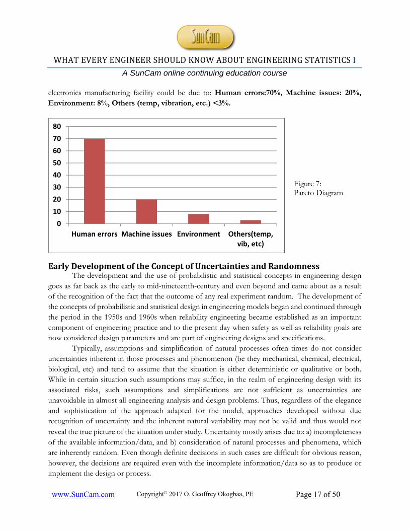
Figure 6: Bar Chart of Number of Nuclear Plants by Country, 2016 4.3.3 Pareto Diagram
Also known as ABC analysis in inventory analysis, the technique is importance because it is sometimes physically impossible (even with the use of computers) to track the hundreds of thousands of items that make up typical inventory systems. In more general terms, it is used to rank occurrences based on their significance or contribution. For example, the cause of errors or defects in an
020406080
100
USA
RUSSIA
FRANCE
GER
MANY
CHINA
JAPAN
INDIA
CANADA
1 2 3 4 5 6 7 8
Number
Country
Number of Nuclear Power Plants by Country 2016
Figure 5: Pie Chart
WHAT EVERY ENGINEER SHOULD KNOW ABOUT ENGINEERING STATISTICS I
A SunCam online continuing education course
www.SunCam.com Copyright 2017 O. Geoffrey Okogbaa, PE Page 17 of 50
electronics manufacturing facility could be due to: Human errors:70%, Machine issues: 20%, Environment: 8%, Others (temp, vibration, etc.) <3%.
EarlyDevelopmentoftheConceptofUncertaintiesandRandomnessThe development and the use of probabilistic and statistical concepts in engineering design
goes as far back as the early to mid-nineteenth-century and even beyond and came about as a result of the recognition of the fact that the outcome of any real experiment random. The development of the concepts of probabilistic and statistical design in engineering models began and continued through the period in the 1950s and 1960s when reliability engineering became established as an important component of engineering practice and to the present day when safety as well as reliability goals are now considered design parameters and are part of engineering designs and specifications.
Typically, assumptions and simplification of natural processes often times do not consider uncertainties inherent in those processes and phenomenon (be they mechanical, chemical, electrical, biological, etc) and tend to assume that the situation is either deterministic or qualitative or both. While in certain situation such assumptions may suffice, in the realm of engineering design with its associated risks, such assumptions and simplifications are not sufficient as uncertainties are unavoidable in almost all engineering analysis and design problems. Thus, regardless of the elegance and sophistication of the approach adapted for the model, approaches developed without due recognition of uncertainty and the inherent natural variability may not be valid and thus would not reveal the true picture of the situation under study. Uncertainty mostly arises due to: a) incompleteness of the available information/data, and b) consideration of natural processes and phenomena, which are inherently random. Even though definite decisions in such cases are difficult for obvious reason, however, the decisions are required even with the incomplete information/data so as to produce or implement the design or process.
0
10
20
30
40
50
60
70
80
Human errors Machine issues Environment Others(temp,vib, etc)
Figure 7: Pareto Diagram
WHAT EVERY ENGINEER SHOULD KNOW ABOUT ENGINEERING STATISTICS I
A SunCam online continuing education course
www.SunCam.com Copyright 2017 O. Geoffrey Okogbaa, PE Page 18 of 50
Decisions in such situations are taken under the condition of uncertainty and thus are understood as such. Hence proper assessment of associated uncertainty is essential, and the effects of such uncertainty in engineering design problems are very crucial in order to quantify the risk envisaged in terms of safety factors and safety margins.
According to Ang and Tang (1975), the role of probability methods in engineering design can be broadly categorized as - a) The modeling of engineering problems and evaluation of systems performance under conditions of uncertainty; b) Systemic development of design criteria, explicitly taking into account the significance of uncertainty, and c) The logical framework for risk assessment and risk benefit trade-off analysis relative to decision making. 5.1 UncertaintyandProbabilityMethods
There are three major types of types of uncertainties that can be associated with any engineering design problem, namely– a) Parameter uncertainties; b) Data uncertainties; c) Operational uncertainties.
5.1.1 Parameteruncertainty Inability to quantify the accuracy of model parameters and inherent variability in model inputs lead to the parameter uncertainty. Moreover, different descriptive statistics, such as the, mean, standard deviation, skewness, among others also vary from one sample data to another. Thus, uncertainties are also associated with these descriptive statistics.
5.1.2 Datauncertainty Error in measurements, problems in consistency and homogeneity of data are known as data uncertainty. Limitations in adequate representation of sample data are addressed by quantifying data uncertainty. Generally, histograms are basic graphical representation of such uncertainty and probability density functions (pdf) are fitted with the histograms to assess the uncertainty associated with the data. These details would be discussed later.
5.1.3 OperationalUncertainties These arise from changes in the operational conditions of structures and errors associated with construction, manufacture, deterioration, maintenance, human activities etc. All the uncertainties are assessed with the help of the concept embodied in the theory of probability. Definitions6.1 Experiment
An experiment is any process or operation that generates raw data, the nature or outcome of which cannot be predicted with certainty. 6.2 Samplespace(S)
A sample space S is the set of all possible outcomes of an experiment.
WHAT EVERY ENGINEER SHOULD KNOW ABOUT ENGINEERING STATISTICS I
A SunCam online continuing education course
www.SunCam.com Copyright 2017 O. Geoffrey Okogbaa, PE Page 19 of 50
6.3 OutcomeAn outcome is one of the set of possible observations which results from the experiment.
One and only one outcome results from one realization of the experiment, e.g., the toss of a fair coin results in the realization of only one outcome, namely, either a head or a tail Examples:
Roll a single die one time. The experiment is the roll of the die. A sample space for this experiment is: S= {1, 2, 3, 4, 5, 6}
A process for making pharmaceutical bottle caps produces 4 types of cap each time the process is completed: the sample space S= {c1, c2, c3, c4}
Select 1 card at random from a deck of 52 cards. The experiment is the selection of the card. If the cards are numbered in a specific order from 1 to 52, then the sample space would be. S= {1, 2, 3, 4, 5, 6, 7,…….., 52 }
6.4 MultipleOutcomesOften an experiment will yield more than one piece of information or more than one outcome
which we may want to use. If we observe 2 pieces of information every time the experiment is performed, we would reasonably want a sample space that is a collection of 2-tuples or two pairs, with the two positions corresponding to the two pieces of information, i.e.
S= {(X1, X2):X1=….., X2=…. } Suppose an experiment consists of one roll of two dice (one red-R, the other green-G). The sample space will be the collection of all possible 2-tuples (X1, X2), where: The number on the first position of the 2-tuple corresponds to the number on the face of the Red die and the other is the number on the face of the Green die, that is
S= DR x DG, where DR = {1, 2, 3, 4, 5, 6} and DG = {1, 2, 3, 4, 5, 6} S= {(X1, X2,): X1=1,2,3,4,5,6; X2=1,2,3,4,5,6}
The total element in this sample space S is 36 (or 6x6) 6.5 Events
An event is a subset of the sample space. Every subset of a sample space is an event. For any experiment, an event occurs if any one of the elements of the event an outcome of the experiment. Consider the toss of a 6-faced die (labeled 1- 6, dice is plural) as an experiment. The sample space is: S = {1, 2, 3, 4, 5, 6} Each of the following subset of the experiment is ALSO AN EVENT, that is:
Let A= {1}, that is the occurrence of a face with 1 Let B= {1,3,5}, that is the occurrence of the faces 1, or 3 or 5 Let C= {2,4,6}, that is the occurrence of the faces 2, 4, 6 or even numbers Let D= {4,5,6}, that is the occurrence of 4, 5, 6 or numbers greater than 3 Let E= {1,3,4,6}, that is any numbers except 2 and 5.
WHAT EVERY ENGINEER SHOULD KNOW ABOUT ENGINEERING STATISTICS I
A SunCam online continuing education course
www.SunCam.com Copyright 2017 O. Geoffrey Okogbaa, PE Page 20 of 50
Please Note: These are not the only events since they are not the only subsets of S. However, note that these events are distinct since no two are equal. For this example, if one were to perform the experiment (roll the die) and get a 1, then the events A, B, and E have occurred since each of these subsets of the experiment contains the number 1. Another example: If we roll a pair of dice one time, the sample space S is the set of all 2-tuples: S = {(X1, X2): X1=1, 2, …6; X2=1, 2..6} One can define the following events, namely:
A: sum of the faces of the two dice is 3,
B: the sum of the faces of the two dice is 7
C: the two dice show the same face. A= {(1,2), (2,1)}, B={(1,6), (2,5), (3,4), 4,3), (5,2),( 6,1)}, C={(1,1), (2,2), (3,3), 4,4), (5,5), 6,6)}
6.6 DefinitionofARandomvariable
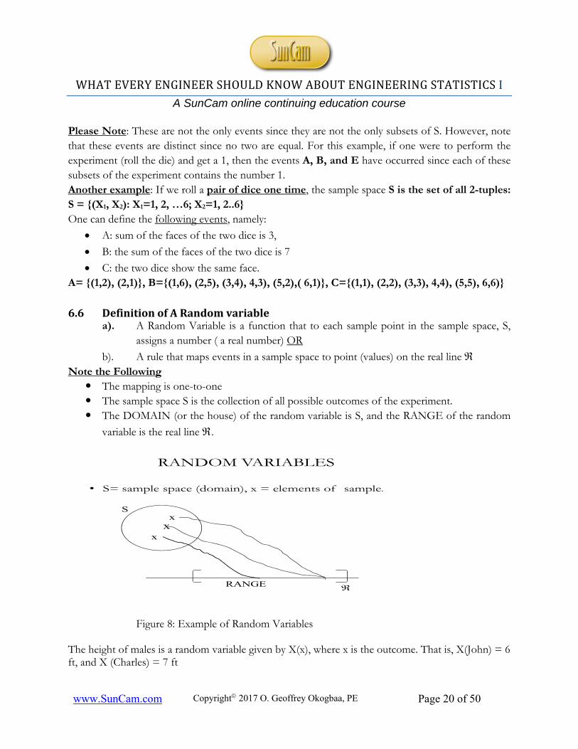
a). A Random Variable is a function that to each sample point in the sample space, S, assigns a number ( a real number) OR
b). A rule that maps events in a sample space to point (values) on the real line Note the Following
The mapping is one-to-one The sample space S is the collection of all possible outcomes of the experiment. The DOMAIN (or the house) of the random variable is S, and the RANGE of the random
variable is the real line .
RANDOM VARIABLES
• S= sample space (domain), x = elements of sample.
x
xx
S
RANGE
Figure 8: Example of Random Variables
The height of males is a random variable given by X(x), where x is the outcome. That is, X(John) = 6 ft, and X (Charles) = 7 ft
WHAT EVERY ENGINEER SHOULD KNOW ABOUT ENGINEERING STATISTICS I
A SunCam online continuing education course
www.SunCam.com Copyright 2017 O. Geoffrey Okogbaa, PE Page 21 of 50
Note: The height of Charles cannot be 7 ft and then 8 ft. Hence, we say that the mapping is unique. Charles can be 7 ft. and so can Andrew. Hence the mapping is unique in one direction (from the domain to the range and not the other way)
DefinitionsofProbability7.1 ClassicalDefinitionofProbability
The classical definition of probability presupposes knowledge of the exact nature of the population from which the sample is drawn. Thus, in a population of N items, if n of those are labeled as successes, then the probability of success is given by: P(success)= n/N Practical Problem with this classical definition approach: We may not know or have access to the population. Quite often only the sample is available. 7.2 RelativeFrequencyDefinition/Approach
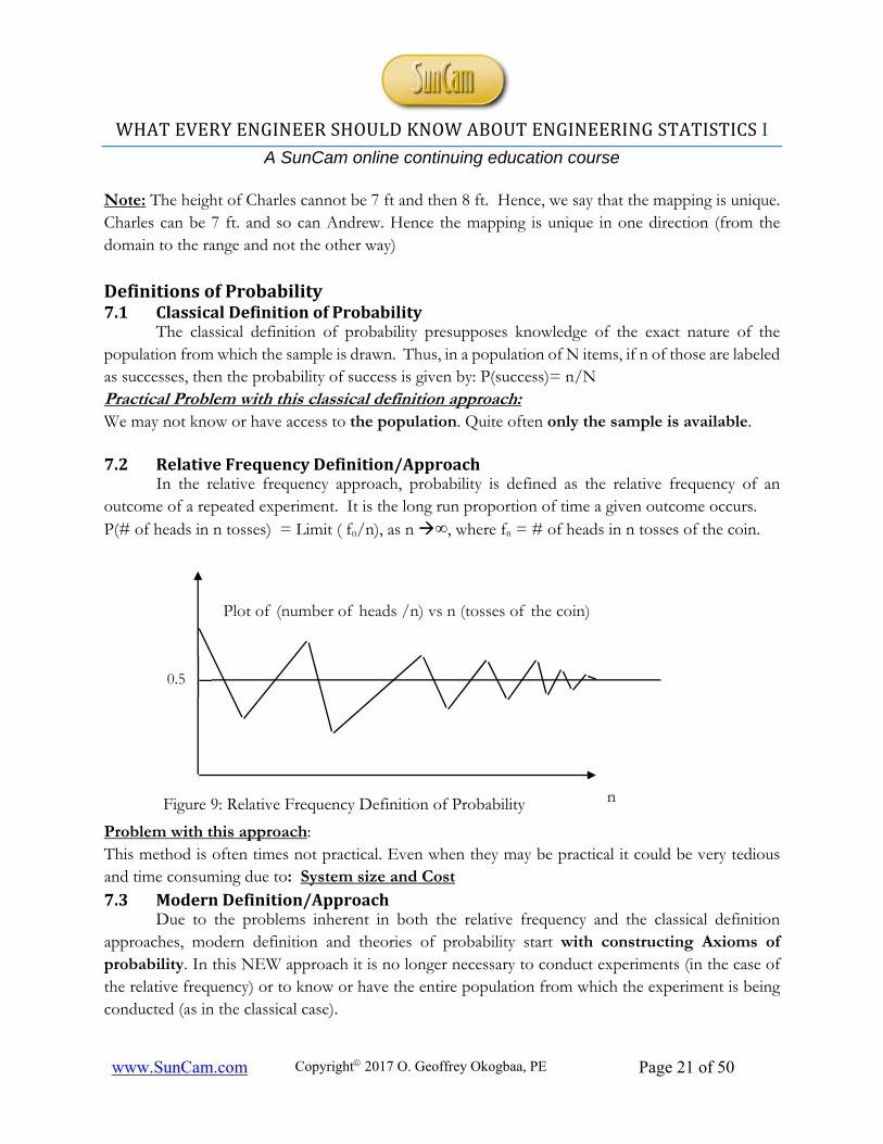
In the relative frequency approach, probability is defined as the relative frequency of an outcome of a repeated experiment. It is the long run proportion of time a given outcome occurs. P(# of heads in n tosses) = Limit ( fn/n), as n ∞, where fn = # of heads in n tosses of the coin.
Problem with this approach: This method is often times not practical. Even when they may be practical it could be very tedious and time consuming due to: System size and Cost 7.3 ModernDefinition/Approach
Due to the problems inherent in both the relative frequency and the classical definition approaches, modern definition and theories of probability start with constructing Axioms of probability. In this NEW approach it is no longer necessary to conduct experiments (in the case of the relative frequency) or to know or have the entire population from which the experiment is being conducted (as in the classical case).
n
0.5
Plot of (number of heads /n) vs n (tosses of the coin)
Figure 9: Relative Frequency Definition of Probability
WHAT EVERY ENGINEER SHOULD KNOW ABOUT ENGINEERING STATISTICS I
A SunCam online continuing education course
www.SunCam.com Copyright 2017 O. Geoffrey Okogbaa, PE Page 22 of 50
7.4 Axioms(orLaws)ofProbability—Addition,Multiplication,InverseThe axioms are then used to construct the general laws of probability.
Let A be an event, and let S be the sample space then. i) 0 ≤ Pr(A) ≤ 1, ii) Pr (s) = 1 7.4.1 Addition Laws Consider two events A and B in S
General Law: P(AՍB) = P(A) + P(B) -P(A∩ B)
Mutually Exclusive Law: P(AՍ B) = P(A) + P(B) In an experiment, two events A, B are Mutually Exclusive if and only if: A ∩ B = Ø, This means that the intersection of A and B is the null set. Hence P (A ∩ B )= 0
so that P(AՍ B) = P(A) + P(B) Note: Mutually Exclusive events are associated with the outcomes of a SINGLE experiment. Also, If the occurrence of one event does not preclude the occurrence of another event in the same experiment, then the two events are mutually exclusive. Note: The events of an experiment forma set for that experiment and the resulting sample space. If the intersection of two or more events associated with the outcome of an experiment is the empty or null set, then the events are said to mutually exclusive. 7.4.2 Multiplication Laws Consider two events A and B in S
Dependent Law: P(A ∩ B)= P(A)P(B|A) Independent Law: P(A ∩ B)= P(A)P(B)
Two events A, B are independent if and only if: P (A ∩ B ) = P(A) P(B). In other words A, B are independent if P(B|A) = P(B). i.e., the occurrence of B does not depend on the occurrence of A. The occurrence of A does not preclude the occurrence of B. Independent events are usually associated with the outcome of two or more experiments 7.4.3 Inverse Law Consider two events A and B in S
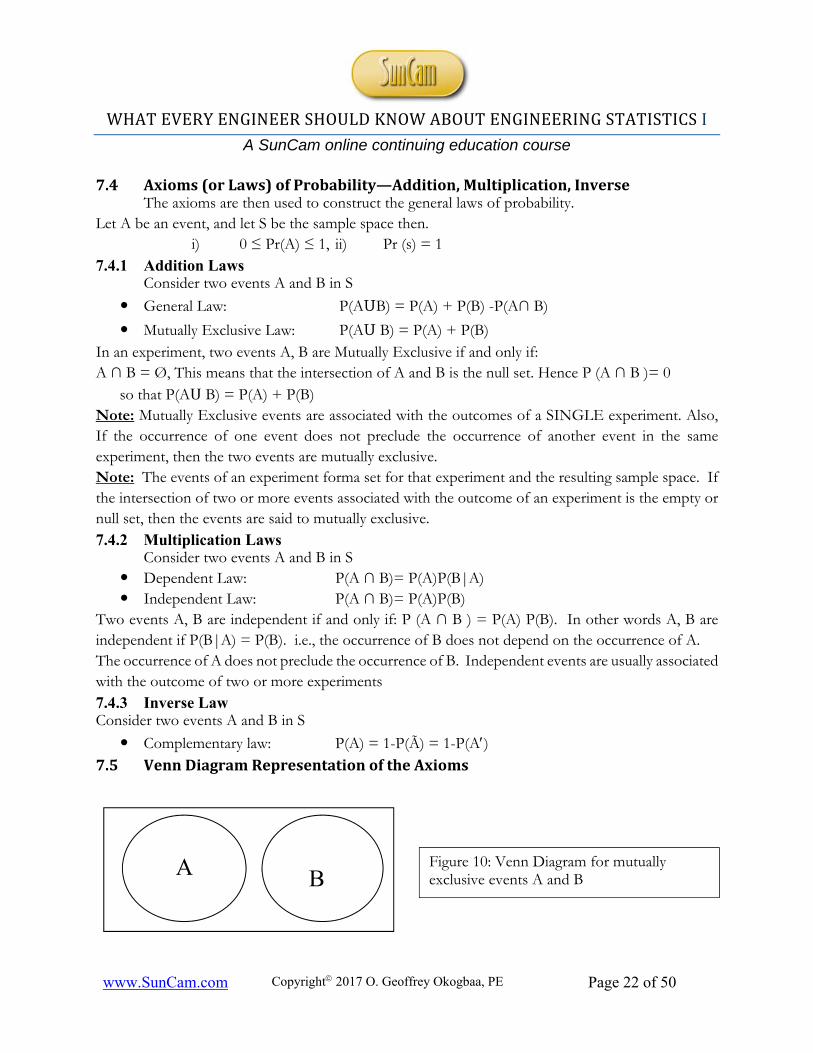
Complementary law: P(A) = 1-P(Ã) = 1-P(A) 7.5 VennDiagramRepresentationoftheAxioms
A B
Figure 10: Venn Diagram for mutually exclusive events A and B
WHAT EVERY ENGINEER SHOULD KNOW ABOUT ENGINEERING STATISTICS I
A SunCam online continuing education course
www.SunCam.com Copyright 2017 O. Geoffrey Okogbaa, PE Page 23 of 50
A and B are mutually exclusive since (AB)=. Hence P(AB )=0. That is to say that ‘A’ intersection ‘B’ is the null set hence the probability of A intersection ‘B’ is zero.
0, DCPDC Analysis with Venn Diagrams
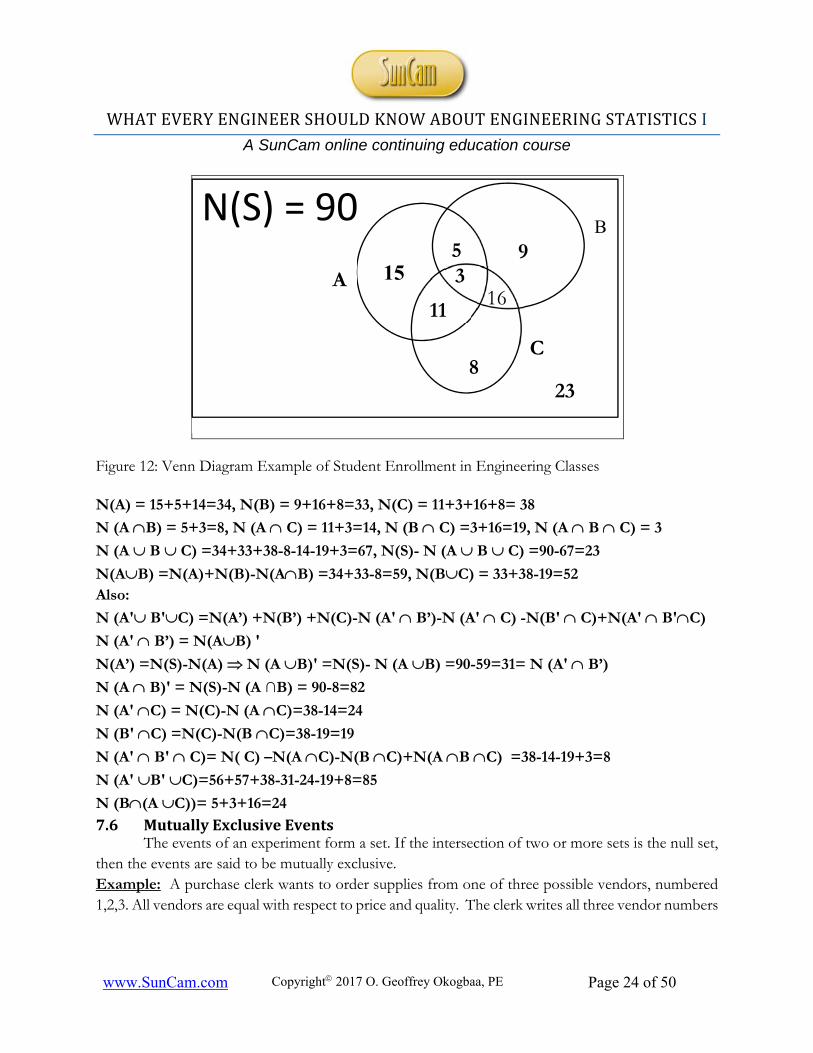
Assume that there 90 members of the engineering honors group Tau Beta PI and we have interest in looking at the different classes taken by the members. Let: Engineering Statistics=A, Linear Systems =B, Computational Methods =C Let the number of students enrolled in A=34, in B=33, in C=38. Those enrolled in A and B=8, and those in A and C=14, and those in B and C=19. Let those enrolled in all three classes=3 Question: Draw the Venn Diagram to represent this scenario. From the Venn Diagram determine how many are not enrolled in any of the three classes?
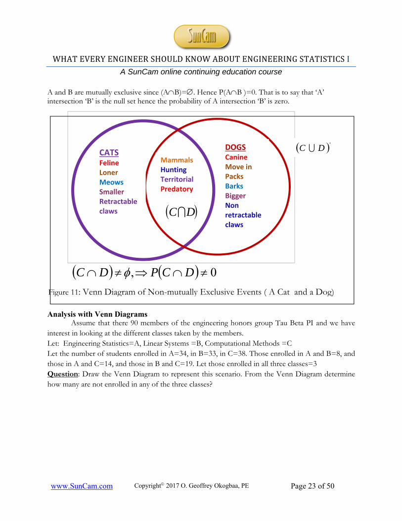
Figure 11: Venn Diagram of Non-mutually Exclusive Events ( A Cat and a Dog)
CATS Feline Loner Meows Smaller Retractable claws
Mammals Hunting Territorial Predatory
DOGS Canine Move in Packs Barks Bigger Non retractable claws
DC
'DC
WHAT EVERY ENGINEER SHOULD KNOW ABOUT ENGINEERING STATISTICS I
A SunCam online continuing education course
www.SunCam.com Copyright 2017 O. Geoffrey Okogbaa, PE Page 24 of 50
Figure 12: Venn Diagram Example of Student Enrollment in Engineering Classes N(A) = 15+5+14=34, N(B) = 9+16+8=33, N(C) = 11+3+16+8= 38
N (A B) = 5+3=8, N (A C) = 11+3=14, N (B C) =3+16=19, N (A B C) = 3
N (A B C) =34+33+38-8-14-19+3=67, N(S)- N (A B C) =90-67=23
N(AB) =N(A)+N(B)-N(AB) =34+33-8=59, N(BC) = 33+38-19=52 Also:
N (A' B'C) =N(A’) +N(B’) +N(C)-N (A' B’)-N (A' C) -N(B' C)+N(A' B'C)
N (A' B’) = N(AB) '
N(A’) =N(S)-N(A) N (A B)' =N(S)- N (A B) =90-59=31= N (A' B’)
N (A B)' = N(S)-N (A ∩B) = 90-8=82
N (A' C) = N(C)-N (A C)=38-14=24
N (B' C) =N(C)-N(B C)=38-19=19
N (A' B' C)= N( C) –N(A C)-N(B C)+N(A B C) =38-14-19+3=8
N (A' B' C)=56+57+38-31-24-19+8=85
N (B(A C))= 5+3+16=24
7.6 MutuallyExclusiveEventsThe events of an experiment form a set. If the intersection of two or more sets is the null set,
then the events are said to be mutually exclusive. Example: A purchase clerk wants to order supplies from one of three possible vendors, numbered 1,2,3. All vendors are equal with respect to price and quality. The clerk writes all three vendor numbers
N(S) = 90
A
B
C
15 35 9
16
8
11
23
WHAT EVERY ENGINEER SHOULD KNOW ABOUT ENGINEERING STATISTICS I
A SunCam online continuing education course
www.SunCam.com Copyright 2017 O. Geoffrey Okogbaa, PE Page 25 of 50
on a piece of paper, mixes paper in a bowl and picks one piece of paper at a time at random. An order is placed with the vendor whose number was selected. Let ei represent vendor i (i=1 to 3). Let B be the event that vendor 1 or 3 is selected and C the event vendor 1 is not selected. Find the following probabilities a). P(Ei), P(B), P(C)
3
2)()()()(
0)(,3
2
3
1
3
1)()()()(
3
1)()()(
)(:
23231
321
3131
3131
21
321
321
EPEPEEPEP
EEEC
EEPEESince
EPEPEEPBP
EEBDefinitionBy
EPEPEP
capabilityequalhavevendorsallEEEGiven
7.7 Non‐MutuallyExclusiveEventsPieces of paper numbered 1 through 9 are mixed together in a bowl. Find the probability that
a number drawn is either even or divisible by 3. Solution Define A= event, number is even Define C=event number is divisible by 3 Based on the sample space S of 9 elements, where S={ 1, 2, 3, 4, 5, 6, 7, 8, 9 } we have: A ε S={2,4,6,8}, C ε S={3,6,9} P(C) =3/9, P(A)= 4/9
AC ={6}, hence P(AC )=1/9
P(AC)= P(A)+P(C)- P(AC )=4/9+3/9-1/9=6/9 7.8 MultiplicationLaw(DependentLaw) From a deck of cards, select 2 cards without replacement. What is the probability that the two cards are Aces? Define A= event Ace in the first draw, Define B= event Ace in the second draw
P(AB)= P(A)P(B|A)= (4/52)(3/51) 7.9 MultiplicationLaw(IndependentLaw) Independent events are associated with the outcome of more than one experimental trial. Thus, the outcome of the present trial does not depend on the outcome of the previous trial. Example: A toss of two coins is made. Show that the events: a) Heads on the 1st coin, and b). Coins fall alike; are independent. S= {HH, HT, TH, TT}, P(HH)=P(HT)=P(TH)=P(TT)=1/4 Event head on 1st coin =A = {HH, HT}, Event head fall alike= B= {HH, TT}
WHAT EVERY ENGINEER SHOULD KNOW ABOUT ENGINEERING STATISTICS I
A SunCam online continuing education course
www.SunCam.com Copyright 2017 O. Geoffrey Okogbaa, PE Page 26 of 50
AB= {HH}=P(A B)=1/4 P(A)= P(HH or HT) = P(HH)+P(HT)=1/4+1/4=1/2 P(B)= P(HH or TT)= P(HH)+P(TT)= 1/4+1/4=1/2, P(A)P(B)=1/2(1/2)=1/4
hence P(AB)=P(A)P(B)=1/4, Thus A and B are independent.
CountingTechniquesOften times it can become tedious if not impossible to determine the number of elements or
the outcomes of a sample space by direct enumeration. Counting techniques are ways in which these enumerations are made without complete listing of all the possibilities. There are several rules that are used to implement such counting, including.
• Multiplication or the m x n rule • Permutation • Combination • General Enumeration • Tree Diagram approach
8.1 MultiplicationorthemxnRuleIf there is an operation that consists of k parts and the 1st can be performed in n1 ways, the
second in n2 ways, the 3rd in n3 way, and…., then the total possible ways of performing the operation is: knnxnxn .....321 If choosing a meal, there
– 5 types of sandwiches or burgers – 4 types of salads – 6 types of fountain drinks – 6 types of desserts
The number of ways of choosing the meal is: 5(4)(6)(6)=720 ways 8.2 Permutation
In general, if r objects are to be chosen from n distinct objects, then any particular arrangement or order of these objects is called permutation.
Thus, in permutation order is important. In the case of telephone numbers or license plates,
the order of the digits is important. For example, the set of digits: 1234 1324 1432 The formula for permutation of r things out of n is given by:
1!1,1!0:
)1)....(3)(2)(1(!:
)!(
!
)!(
)!)(1)...(2)(1(
andNote
nnnnnnnWhere
rn
n
rn
rnrnnnnPr
n
Some quick notes on permutation: 0! =1, 1! =1 , 2! =2(1)=2, 6!=(6)5!=6(5)4!, and so on, 6!= 6(5)(4)(3)(2)(1)= 720
WHAT EVERY ENGINEER SHOULD KNOW ABOUT ENGINEERING STATISTICS I
A SunCam online continuing education course
www.SunCam.com Copyright 2017 O. Geoffrey Okogbaa, PE Page 27 of 50
How many different ways can a local chapter of ASCE schedule 3 speakers for three different meetings if they are all available on any of 5 possible dates.
60!2
!2)3)(4)(5(
)!35(
!53
5
P
Example: Suppose we want to find the total count of the 4-digit numbers that can be formed from the digits: 1,2,3,4,5 if no digit is repeated
Using the formula for permutation, we have: 120)1)(2)(3)(4(5!5)!45(
!54
5
P
There will be 120 4-digit numbers with no repeats. If repeats are allowed, then the no. of 4-digit numbers will be 54. 8.3 Combination If in the enumeration or counting, there is no regard for the order then we have combination instead of permutation. For example, in combination: 123=231=321=312. Because of the disregard for order, combination is numerically less than permutation. The formula for combination is given as:
!)!(
!
rrn
nn
r
Suppose want to select 3 out of five of my favorite books on the shelf (labeled A-E) to read on a weekend trip. In how many ways can this be done?
10!3!2
!3)4(5
!3!)35(
!5
!!)(
! 5
3
rrn
nn
r
The 10 Combinations are:
CADCDEBCEBCDBDE
ACEABDADEABEABC
WHAT EVERY ENGINEER SHOULD KNOW ABOUT ENGINEERING STATISTICS I
A SunCam online continuing education course
www.SunCam.com Copyright 2017 O. Geoffrey Okogbaa, PE Page 28 of 50
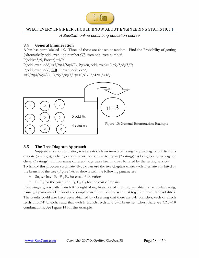
8.4 GeneralEnumerationA bin has parts labeled 1-9. Three of these are chosen at random. Find the Probability of getting (Alternatively odd, even odd number OR even odd even number) P(odd)=5/9, P(even)=4/9 P(odd, even, odd)=(5/9)(4/8)(4/7), P(even, odd, even)=(4/9)(5/8)(3/7) P(odd, even, odd) OR P(even, odd, even) =(5/9)(4/8)(4/7)+(4/9)(5/8)(3/7)=10/63+5/42=(5/18)
8.5 TheTreeDiagramApproach
Suppose a consumer testing service rates a lawn mower as being easy, average, or difficult to operate (3 ratings); as being expensive or inexpensive to repair (2 ratings); as being costly, average or cheap (3 ratings). In how many different ways can a lawn mower be rated by the testing service? To handle this problem systematically, we can use the tree-diagram where each alternative is listed as the branch of the tree (Figure 14). as shown with the following parameters
• So, we have E1, E2, E3 for ease of operation • P1, P2 for the price, and C1, C2, C3 for the cost of repairs
Following a given path from left to right along branches of the tree, we obtain a particular rating, namely, a particular element of the sample space, and it can be seen that together there 18 possibilities. The results could also have been obtained by observing that there are 3-E branches, each of which feeds into 2-P branches and that each P branch feeds into 3–C branches. Thus, there are 3.2.3=18 combinations. See Figure 14 for this example.
1 2 3
4 5 6
7 8 9
n=3
5 odd #s
4 even #s Figure 13: General Enumeration Example

WHAT EVERY ENGINEER SHOULD KNOW ABOUT ENGINEERING STATISTICS I
A SunCam online continuing education course
www.SunCam.com Copyright 2017 O. Geoffrey Okogbaa, PE Page 29 of 50
Figure 14: Tree Diagram for rating lawn Mowers
E1
E2
E3
P1
P2
P1
P2
P1
P2
C1
C2
C3
C3
C2
C1
C1
C2 C3
C1
C2
C3
C1
C2
C3
C1
C2
WHAT EVERY ENGINEER SHOULD KNOW ABOUT ENGINEERING STATISTICS I
A SunCam online continuing education course
www.SunCam.com Copyright 2017 O. Geoffrey Okogbaa, PE Page 30 of 50
Upper Branch
Game Wins
4 1 5 4 6 10
7 20 35
2 Branches =2x35=70
8 Wins in 5 games
NNNAN NNANN Upper NANNN NAAAA
AAANA AANAA Lower ANAAA ANNNN
Win in 6 games Upper Branch
NNNAAN NNANAN NNAANN NNAAAA NANNAN NANANN NANAAA NAANNN NAANAA NAAANA
game game game game game game game 1 2 3 4 5 6 7
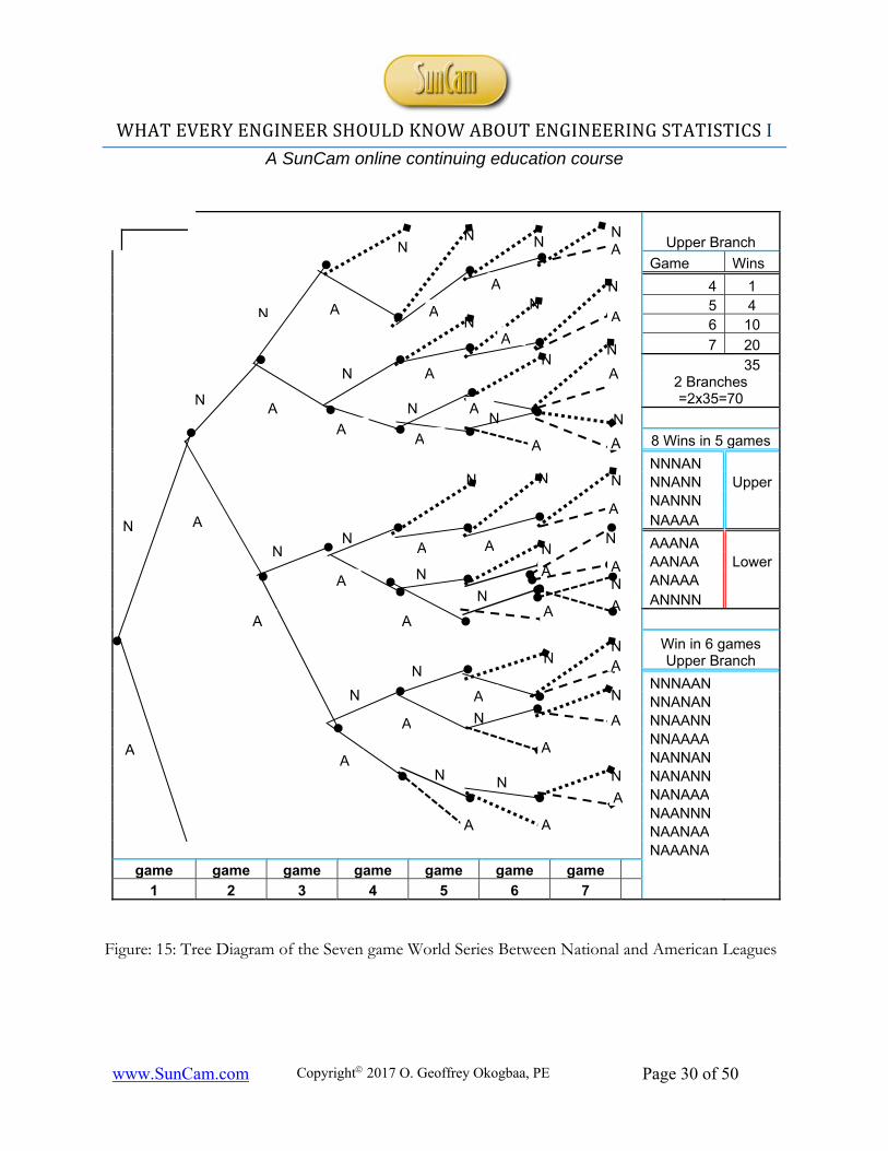
Figure: 15: Tree Diagram of the Seven game World Series Between National and American Leagues
N
N
N
N
A
A
A
A
A
A
N
N
N
N
N
A
AN
A
A
N
N
A
N
A
N
A
NA
A
N
A
A
N
N
A
N A
A
N
N
A
A
N
A
A
AN
N
N
A
N
A
N
A
NA
A
N N
A
N
A
N
A
A
N
A
N
N
WHAT EVERY ENGINEER SHOULD KNOW ABOUT ENGINEERING STATISTICS I
A SunCam online continuing education course
www.SunCam.com Copyright 2017 O. Geoffrey Okogbaa, PE Page 31 of 50
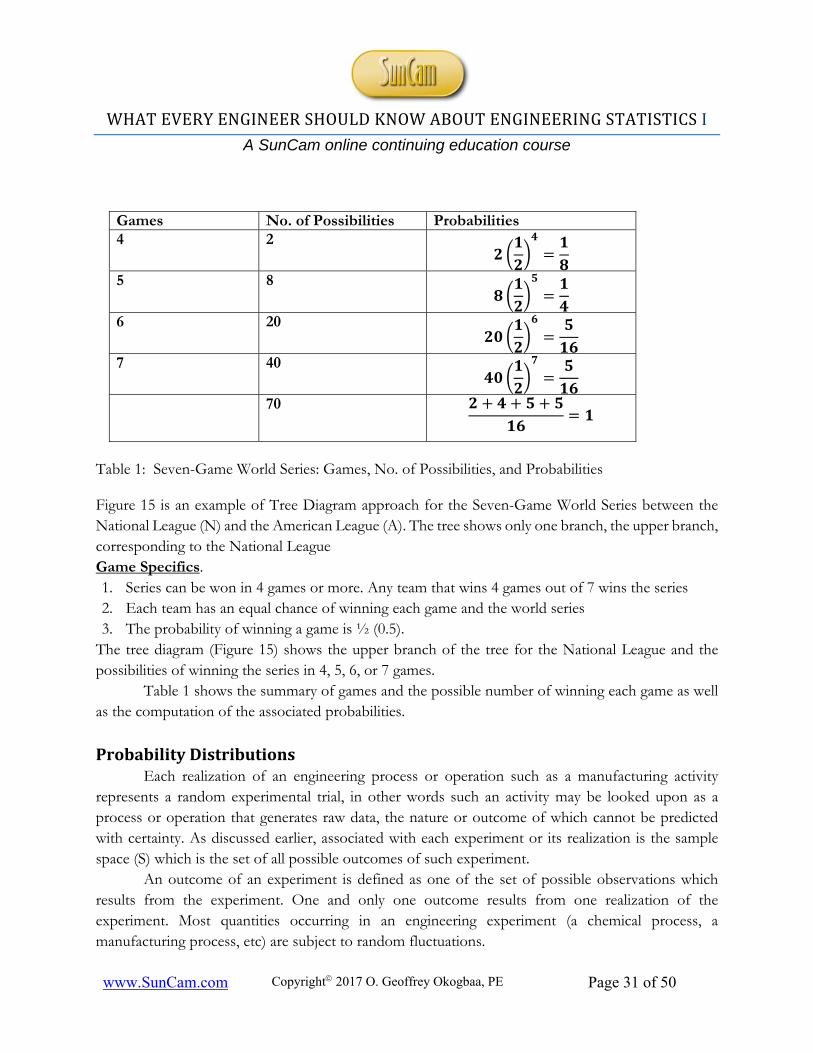
Games No. of Possibilities Probabilities 4 2
𝟐𝟏𝟐
𝟒 𝟏𝟖
5 8 𝟖
𝟏𝟐
𝟓 𝟏𝟒
6 20 𝟐𝟎
𝟏𝟐
𝟔 𝟓𝟏𝟔
7 40 𝟒𝟎
𝟏𝟐
𝟕 𝟓𝟏𝟔
70 𝟐 𝟒 𝟓 𝟓𝟏𝟔
𝟏
Table 1: Seven-Game World Series: Games, No. of Possibilities, and Probabilities Figure 15 is an example of Tree Diagram approach for the Seven-Game World Series between the National League (N) and the American League (A). The tree shows only one branch, the upper branch, corresponding to the National League Game Specifics. 1. Series can be won in 4 games or more. Any team that wins 4 games out of 7 wins the series 2. Each team has an equal chance of winning each game and the world series 3. The probability of winning a game is ½ (0.5).
The tree diagram (Figure 15) shows the upper branch of the tree for the National League and the possibilities of winning the series in 4, 5, 6, or 7 games.
Table 1 shows the summary of games and the possible number of winning each game as well as the computation of the associated probabilities.
ProbabilityDistributionsEach realization of an engineering process or operation such as a manufacturing activity
represents a random experimental trial, in other words such an activity may be looked upon as a process or operation that generates raw data, the nature or outcome of which cannot be predicted with certainty. As discussed earlier, associated with each experiment or its realization is the sample space (S) which is the set of all possible outcomes of such experiment.
An outcome of an experiment is defined as one of the set of possible observations which results from the experiment. One and only one outcome results from one realization of the experiment. Most quantities occurring in an engineering experiment (a chemical process, a manufacturing process, etc) are subject to random fluctuations.
WHAT EVERY ENGINEER SHOULD KNOW ABOUT ENGINEERING STATISTICS I
A SunCam online continuing education course
www.SunCam.com Copyright 2017 O. Geoffrey Okogbaa, PE Page 32 of 50
Because of the fluctuation and the randomness of the experiments, the outcomes are random variables. In order to characterize these random variables so that they can become useful tools in describing an engineering operation or process, it is important to understand what random variables really are. 9.1 RandomVariables
Definition
A random variable is a function that to each sample point in the sample space, S, assigns a number (a real number) Or
A rule that maps events in a sample space to point (values) on the real line Random variables in general are subject to random fluctuations and they exhibit certain
regularities and sometimes they may have well defined forms. In some cases, they are also of a given form or belong to some class or family. Thus, depending on the type of random experiment that
generated the domain of the random variable, the mapping or assignment to the real line can be generalized into closed form expressions, formulas, equations, rules or graphs that describe how the values are assigned. Note the following
The mapping is one-to-one
The sample space S is the collection of all possible outcomes of the experiment.
The DOMAIN of the random variable is S, and the RANGE of the random variable
is the real line . An intuitive definition of a random variable is that it is a quantity that takes on real values randomly.
An operating definition of a random variable is that it is a function that, to each sample point
in the sample space S, assigns a real value a number on the real line. In other words, the random
variable maps the sample space onto a real value on the real line. Because of its nature and the inherent characteristics, such a variable can be described as
random. Thus, the random variable can be expressed as the function: X ( x) = a numerical value equal to the height of a unique individual male named x, i.e., X
(John1) = 6 ft, X (Paul20) = 7ft, X (Don10) =6 ft, where in this case X is the random variable that assigns the value 6ft to John1, and 7ft. to Paul20.
Please note that two elements from the sample space can have the same real values assigned to them. In our example, John1 and Don10 have the same height. However, John1 cannot have heights of 6 ft. and 7 ft. at the same time, hence the mapping is unique in one direction, why? 9.2 DomainandRangeofaRandomVariable
The domain of the random variable is the sample space (S) and the range of the random
variable is the real line . It is the range of the random variable that determines the types of values that are assigned to the random variable under consideration. A more general definition of a random
WHAT EVERY ENGINEER SHOULD KNOW ABOUT ENGINEERING STATISTICS I
A SunCam online continuing education course
www.SunCam.com Copyright 2017 O. Geoffrey Okogbaa, PE Page 33 of 50
variable (RV) is that it can take on any values on the real line . A real-valued random variable may assume one of the following:
(a) Two possible values. For example, in the case of product quality, the values could be 1 if the product is conforming and 0 if it does not conform.
(b) A finite number of values. If the face of a die is assumed to be random variable in some experiment, then the possible numbers are 1 through 6.
(c ) Also in the case of product quality, the number of nonconforming items in a lot is finite and will never be more than the lot size even in the worst case scenario.
(d) Countably infinite discrete values. (The number of telephone calls made in a given time epoch all over the world).
(e ) Any value on the interval on the real line . For example, the weight of a container in a filling operation
(f) Any value in a half infinite interval on the real line (the strength of a component may take values in the interval (0, infinity]. These values that are possible for any random variable determine whether a random variable
can be classified as discrete or continuous. A typical discrete random variable is one that takes on the first three values (a-c), whereas continuous random variables take on values as defined in the last three, namely, (d-f). 9.3 RulesorEquationsforMapping/Assignment
These rules or equations for mapping or assignment from the domain to the real line are known as probability density functions (for continuous random variables) and probability mass functions (for discrete random variables). In other words, probability density or mass functions are simply closed form expressions or rules that indicate how assignments to values on the real line are made from the domain of the random variable.
The nature of the experiment ultimately determines the type of equations or rules that apply. For example, one of the problems associated with using the density function to characterize a manufacturing process or chemical process is that in some cases such closed form expression or equation are difficult to come by. Hence one is often left to make assumptions using the average value from the data obtained from the experiment or some measure of the variability obtained from which is often measured with the variance or standard deviation or the range. The mean and standard deviation from the experimental data are referred to as the first and second moments.
Usually the first and second moments (the mean and variance) do provide enough useful insight as to the behavior of the random variable. However, in some cases these parameters (the mean and the standard deviation or variance) are not enough to completely characterize the underlying random variable and so one has to look to other approaches that would provide the confidence needed to ensure that indeed the equation or function assumed is the appropriate one.
WHAT EVERY ENGINEER SHOULD KNOW ABOUT ENGINEERING STATISTICS I
A SunCam online continuing education course
www.SunCam.com Copyright 2017 O. Geoffrey Okogbaa, PE Page 34 of 50
These are closed form expressions or equation that is used to characterize the ransom variable. Probability distribution or Probability Density or mass Functions are closed form expressions that used to typify the behavior of a particular random variable. Based on our definition of the range of random variables, we have two distinct type, namely, discrete and continuous. We will examine those subsequently. DiscreteRandomvariables
Discrete Random variables are those that assume: i) Finite or ii)Countably infinite values. (The number of telephone calls made in all over the world in a
given year). A typical discrete random variable is one that takes finite values on the real line, eg. 0 or 1, good bad,
go-no-go, etc. A random variable X is called discrete if its range x is a discrete set of real numbers. Example: We roll a pair of dice 1 time. Let x be the sum of the 2 numbers that occur. Then we have the sample space:
S={(x1,, x2): x1=1, 2, …6; x2=1, 2,…6}, X()= x1,+x2, for =(x1,,x2) S
The range of X is x ={2, 3, …12} so X is a discrete R.V
Example: A sample of 3 people is selected at random from the list of registered voters in Hillsborough County, FL. Let Y be the number of Republicans that occur in that sample of 3. For convenience, we use as our sample space the following: S= {(x1, x2 , x3): x1=0, 1; x2 =0,1; x3=0, 1} Let the proportion of Republican voters Hillsborough County be 0.4. Also, assume that the number of registered voters is large very large compared to the sample and so the probability of selecting a Republican equal to 0.4. Therefore,
P{x=1(prob. of Republican)}=0.4; and P{(x=0(prob. not Republican)} =0.6 Then we have the following probabilities:
P{(0,0,0)}=(0.6)3 , P{(1,0,0)}=(0.4)(0.6)2 P{(0,1,0)}=(0.6)(0.4)(0.6), P{(1,1,1)}=(0.4)3
The range of Y, the Republicans who appear in the sample is {0,1,2,3}, we define the following: A (0)= {(0,0,0)} ; A(1)= {(1,0,0), (0,1,0), (0,0,1)}, A(2)= {(1,1,0), (1,0,1), (0,1,1)} ; A (3)= {(1,1,1)} The probability function Y which gives the number of Republicans selected in the sample is given by:
Y=0, pY(y=0) = (0.6)3=0.216= P[A(0)] No Republican selected
Y=1, pY(y=1)= P[A(1)]=(0.4)(0.6)2+(0.6)(0.4)(0.6)+(0.6)2(0.4)=0.432 One Republican Selected
Y=2, pY(y=2)= P[A(2)]=(0.4)2(0.6) +(0.4)(0.6)(0.4)+(0.6) (0.4)2=0.288 Only two selected
Y=3, pY(y=3)=P[A(3)]=(0.4)3 =0.064 Three Republicans selected.
WHAT EVERY ENGINEER SHOULD KNOW ABOUT ENGINEERING STATISTICS I
A SunCam online continuing education course
www.SunCam.com Copyright 2017 O. Geoffrey Okogbaa, PE Page 35 of 50
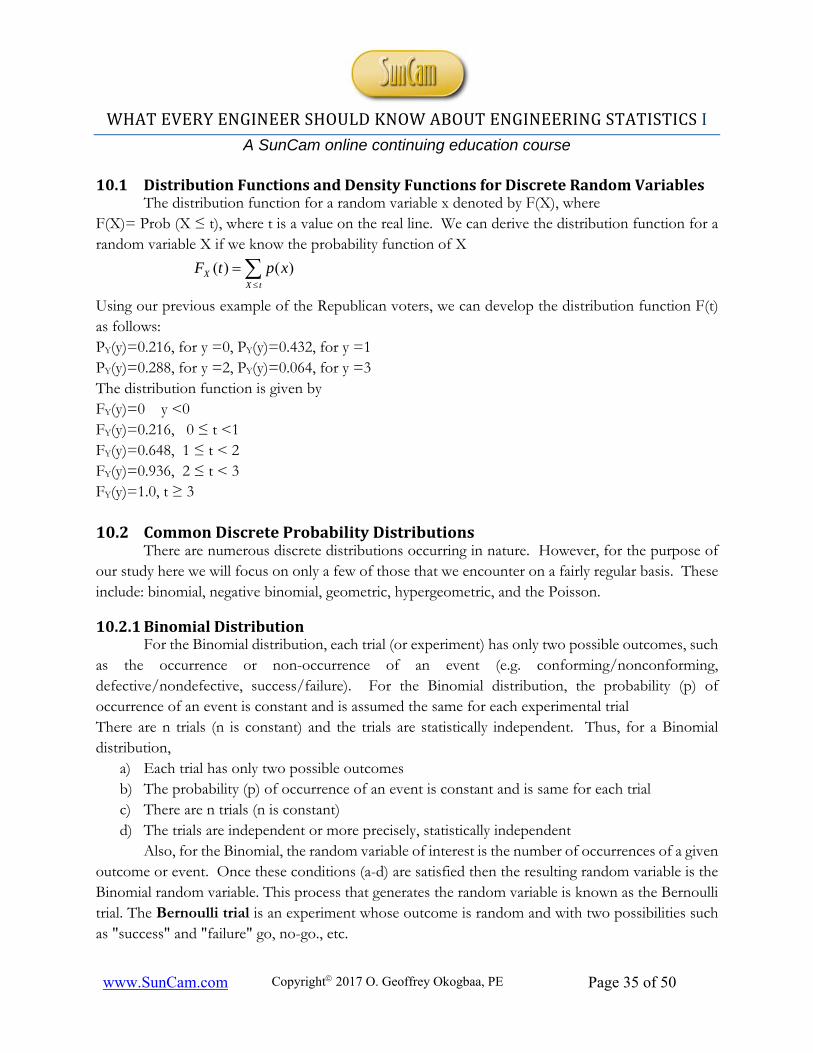
10.1 DistributionFunctionsandDensityFunctionsforDiscreteRandomVariablesThe distribution function for a random variable x denoted by F(X), where
F(X)= Prob (X ≤ t), where t is a value on the real line. We can derive the distribution function for a random variable X if we know the probability function of X
tX
X xptF )()(
Using our previous example of the Republican voters, we can develop the distribution function F(t) as follows: PY(y)=0.216, for y =0, PY(y)=0.432, for y =1 PY(y)=0.288, for y =2, PY(y)=0.064, for y =3 The distribution function is given by FY(y)=0 y <0 FY(y)=0.216, 0 ≤ t <1 FY(y)=0.648, 1 ≤ t < 2 FY(y)=0.936, 2 ≤ t < 3 FY(y)=1.0, t ≥ 3 10.2 CommonDiscreteProbabilityDistributions
There are numerous discrete distributions occurring in nature. However, for the purpose of our study here we will focus on only a few of those that we encounter on a fairly regular basis. These include: binomial, negative binomial, geometric, hypergeometric, and the Poisson.
10.2.1BinomialDistributionFor the Binomial distribution, each trial (or experiment) has only two possible outcomes, such
as the occurrence or non-occurrence of an event (e.g. conforming/nonconforming, defective/nondefective, success/failure). For the Binomial distribution, the probability (p) of occurrence of an event is constant and is assumed the same for each experimental trial There are n trials (n is constant) and the trials are statistically independent. Thus, for a Binomial distribution,
a) Each trial has only two possible outcomes b) The probability (p) of occurrence of an event is constant and is same for each trial c) There are n trials (n is constant) d) The trials are independent or more precisely, statistically independent
Also, for the Binomial, the random variable of interest is the number of occurrences of a given outcome or event. Once these conditions (a-d) are satisfied then the resulting random variable is the Binomial random variable. This process that generates the random variable is known as the Bernoulli trial. The Bernoulli trial is an experiment whose outcome is random and with two possibilities such as "success" and "failure" go, no-go., etc.
WHAT EVERY ENGINEER SHOULD KNOW ABOUT ENGINEERING STATISTICS I
A SunCam online continuing education course
www.SunCam.com Copyright 2017 O. Geoffrey Okogbaa, PE Page 36 of 50
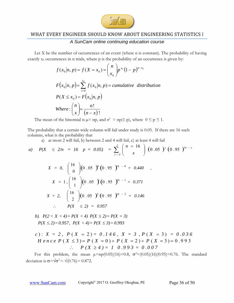
Let X be the number of occurrences of an event (where n is constant). The probability of having exactly x0 occurrences in n trials, where p is the probability of an occurrence is given by:
!
!:
,)(
),(,
1)(),(
00
000
000
0
00
xn
n
x
nWhere
pnxFxXP
ondistributicumulativepnxfpnxF
ppx
nxXfpnxf
x
i
xnx
The mean of the binomial is µ= np, and σ2 = np(1-p), where 0 ≤ p ≤ 1. The probability that a certain wide column will fail under study is 0.05. If there are 16 such columns, what is the probability that
a) at most 2 will fail, b) between 2 and 4 will fail, c) at least 4 will fail
xx2
0=x x
n = 0.05)=p 16=2/nP(X a)
1695.005.0
16
0.993 = 3)P(X = 4)<P(X0.957 = 2)P(X
3)=P(X = 2)P(X 4)<P(X = 4)<X<P(2 b)
,
.
) : ( 2 ) , , ( 3 )
( 3 ) ( 0 ) ( 2 ) ( 3 ) 0 . 9 9 3c X = 2 , P X = 0 . 1 4 6 X = 3 P X = 0 . 0 3 6
H e n c e P X P X P X P XP ( X 4 ) = 1 0 . 9 9 3 = 0 . 0 0 7
For this problem, the mean μ=np(0.05)(16)=0.8, 2=(0.05)(16)(0.95)=0.76. The standard
deviation is =2 = (0.76)= 0.872.
0.957 = 2)P(X
0.146 = 2,=X
0.371= ,=X
0.440 = 0,=X
2162
1161
0160
95.005.02
16
95.005.01
161
,95.005.00
16
WHAT EVERY ENGINEER SHOULD KNOW ABOUT ENGINEERING STATISTICS I
A SunCam online continuing education course
www.SunCam.com Copyright 2017 O. Geoffrey Okogbaa, PE Page 37 of 50
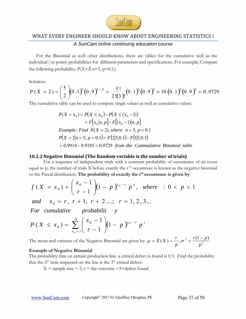
For the Binomial as well other distributions, there are tables for the cumulative well as the individual ( or point) probabilities for different parameters and specifications. For example; Compute
the following probability; P(X=2n=5, p=0.1); Solution:
0729.09.01.0109.01.0!3!2
!59.01.02
5)2( 3232252
XP
The cumulative table can be used to compute single values as well as cumulative values.
tableBinomialeCummulativthefrom
FFpnXP
pnwhereXPFindExample
pnxFpnxF
xXPxXPxXP
0729.09185.09914.0
1.0,511.0,521.0,52
1.0,5),2(:
,)1(,
)1()(
00
000
10.2.2NegativeBinomial(TheRandomvariableisthenumberoftrials)For a sequence of independent trials with a constant probability of occurrence of an event
equal to p, the number of trials X before exactly the r th occurrence is known as the negative binomial or the Pascal distribution. The probability of exactly the rth
occurrence is given by:
X
rx
rrx
rrx
ppr
xxXP
yprobabilitcumulativeFor
rrrrxand
pwhereppr
xxXf
0
0
0
11
1)(
,..3,2,1....;2,1,
10:,11
1)(
00
0
00
The mean and variance of the Negative Binomial are given by: 2
2 )1(,)(
p
pr
p
rXE
Example of Negative Binomial The probability that on certain production line, a critical defect is found is 0.3. Find the probability that the 5th item inspected on the line is the 3th critical defect.
X = sample size = 5, r = the outcome =3=defect found
WHAT EVERY ENGINEER SHOULD KNOW ABOUT ENGINEERING STATISTICS I
A SunCam online continuing education course
www.SunCam.com Copyright 2017 O. Geoffrey Okogbaa, PE Page 38 of 50
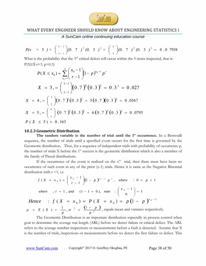
7938.037375 324
2
3215
13
0)(0.)(0. = )(0.)(0. = ) = P(x
What is the probability that the 3rd critical defect will occur within the 5 items inspected, that is:
P(X5r=3, p=0.3)
5
00
0
011
1)(
rx
rrx ppr
xxXP
027.03.03.07.0,3 33013
13
X
163.0)5(
0793.03.07.063.07.0,5
0567.03.07.033.07.0,4
32324
2
3313
2
XP
X
X
10.2.3GeometricDistributionThe random variable is the number of trial until the 1st occurrence. In a Bernoulli
sequence, the number of trials until a specified event occurs for the first time is governed by the Geometric distribution. Thus, for a sequence of independent trials with probability of occurrence p, the number of trials X before the 1st success is the geometric distribution which is also a member of the family of Pascal distributions.
If the occurrence of the event is realized on the xth trial, then there must have been no occurrence of such event in any of the prior (x-1) trials. Hence it is same as the Negative Binomial distribution with r =1, i.e
10
1:),011(,1;
10:,11
1)(
0
00
0
xnoteandrwhere
pwhereppr
xxXf rrx
100
01)()(: xppxXPxXfHence
22 1
,1
)(p
p
pXE
, equals mean and variance respectively.
The Geometric Distribution is an important distribution especially in process control when goal to determine the average run length (ARL) before we detect failure or critical defect. The ARL refers to the average number inspections or measurements before a fault is detected. Assume that X is the number of trials, inspections or measurements before we detect the first failure or defect. This
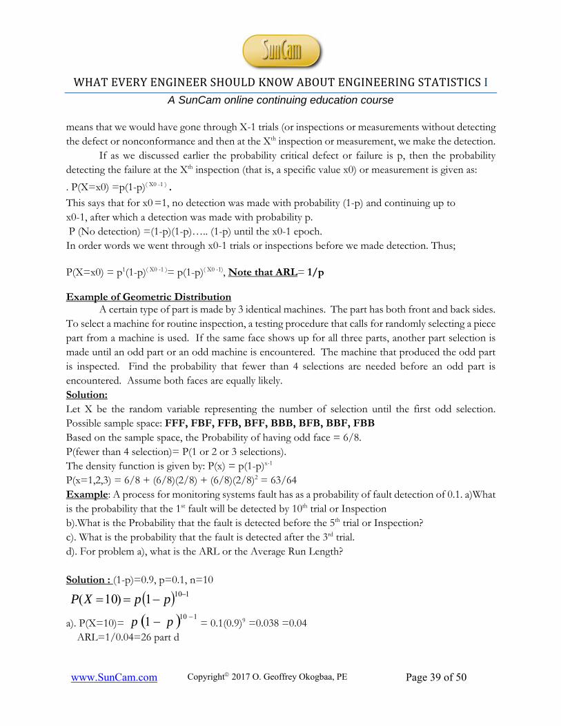
WHAT EVERY ENGINEER SHOULD KNOW ABOUT ENGINEERING STATISTICS I
A SunCam online continuing education course
www.SunCam.com Copyright 2017 O. Geoffrey Okogbaa, PE Page 39 of 50
means that we would have gone through X-1 trials (or inspections or measurements without detecting the defect or nonconformance and then at the Xth inspection or measurement, we make the detection.
If as we discussed earlier the probability critical defect or failure is p, then the probability detecting the failure at the Xth inspection (that is, a specific value x0) or measurement is given as:
. P(X=x0) =p(1-p)( X0 -1 ) . This says that for x0 =1, no detection was made with probability (1-p) and continuing up to x0-1, after which a detection was made with probability p. P (No detection) =(1-p)(1-p)….. (1-p) until the x0-1 epoch. In order words we went through x0-1 trials or inspections before we made detection. Thus; P(X=x0) = p1(1-p)( X0 -1 )= p(1-p)( X0 -1), Note that ARL= 1/p Example of Geometric Distribution
A certain type of part is made by 3 identical machines. The part has both front and back sides. To select a machine for routine inspection, a testing procedure that calls for randomly selecting a piece part from a machine is used. If the same face shows up for all three parts, another part selection is made until an odd part or an odd machine is encountered. The machine that produced the odd part is inspected. Find the probability that fewer than 4 selections are needed before an odd part is encountered. Assume both faces are equally likely. Solution: Let X be the random variable representing the number of selection until the first odd selection. Possible sample space: FFF, FBF, FFB, BFF, BBB, BFB, BBF, FBB Based on the sample space, the Probability of having odd face = 6/8. P(fewer than 4 selection)= P(1 or 2 or 3 selections). The density function is given by: P(x) = p(1-p)x-1 P(x=1,2,3) = 6/8 + (6/8)(2/8) + (6/8)(2/8)2 = 63/64 Example: A process for monitoring systems fault has as a probability of fault detection of 0.1. a)What is the probability that the 1st fault will be detected by 10th trial or Inspection b).What is the Probability that the fault is detected before the 5th trial or Inspection? c). What is the probability that the fault is detected after the 3rd trial. d). For problem a), what is the ARL or the Average Run Length? Solution : (1-p)=0.9, p=0.1, n=10
1101)10( ppXP
a). P(X=10)= 1101 pp = 0.1(0.9)9 =0.038 =0.04 ARL=1/0.04=26 part d
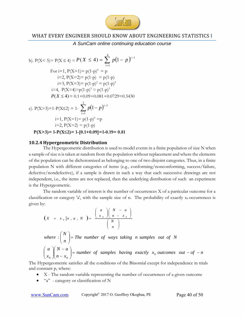
WHAT EVERY ENGINEER SHOULD KNOW ABOUT ENGINEERING STATISTICS I
A SunCam online continuing education course
www.SunCam.com Copyright 2017 O. Geoffrey Okogbaa, PE Page 40 of 50
b). P(X< 5)= P(X 4) =
4
1
11)4(i
ippXP
For i=1, P(X=1)= p(1-p)0 = p i=2, P(X=2)= p(1-p) = p(1-p) i=3, P(X=3)= p(1-p)2 = p(1-p)2
i=4, P(X=4)=p(1-p)3 = p(1-p)3 )4( XP = 0.1+0.09+0.081+0.0729=0.3430
c). P(X>3)=1-P(X2) = 1-
2
1
11i
ipp
i=1, P(X=1)= p(1-p)0 =p i=2, P(X=2) = p(1-p)
P(X>3)= 1-P(X2)= 1-[0.1+0.09]=1-0.19= 0.81
10.2.4HypergeometricDistributionThe Hypergeometric distribution is used to model events in a finite population of size N when
a sample of size n is taken at random from the population without replacement and where the elements of the population can be dichotomized as belonging to one of two disjoint categories. Thus, in a finite population N with different categories of items (e.g., conforming/nonconforming, success/failure, defective/nondefective), if a sample is drawn in such a way that each successive drawings are not independent, i.e., the items are not replaced, then the underlying distribution of such an experiment is the Hypergeometric.
The random variable of interest is the number of occurrences X of a particular outcome for a classification or category 'a', with the sample size of n. The probability of exactly x0 occurrences is given by:
n
N
xn
aN
x
a
NanxX 000 ,,
nofoutoutcomesxexactlyhavingsamplesofnumberxn
aN
x
a
NofoutsamplesntakingwaysofnumberThen
Nwhere
000
:
The Hypergeometric satisfies all the conditions of the Binomial except for independence in trials and constant p, where:
X - The random variable representing the number of occurrences of a given outcome “a” - category or classification of N
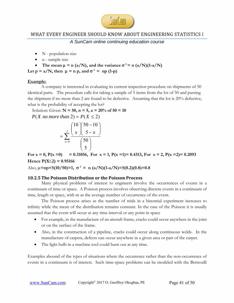
WHAT EVERY ENGINEER SHOULD KNOW ABOUT ENGINEERING STATISTICS I
A SunCam online continuing education course
www.SunCam.com Copyright 2017 O. Geoffrey Okogbaa, PE Page 41 of 50
N - population size n - sample size The mean = n (a/N), and the variance 2 = n (a/N)(1-a/N)
Let p = a/N, then = n p, and 2 = np (1-p) Example:
A company is interested in evaluating its current inspection procedure on shipments of 50 identical parts. The procedure calls for taking a sample of 5 items from the lot of 50 and passing the shipment if no more than 2 are found to be defective. Assuming that the lot is 20% defective, what is the probability of accepting the lot?
Solution: Given: N = 50, n = 5, a = 20% of 50 = 10
2
0
5
50
5
105010
)2()2(
x
xx
XPthanmorenoXP
For x = 0, P(x =0) = 0.31056, For x = 1, P(x =1)= 0.4313, For x = 2, P(x =2)= 0.2093
Hence P(X2) = 0.95166
Also, =np=5(10/50)=1, 2 = n (a/N)(1-a/N)=5(0.2)(0.8)=0.8
10.2.5ThePoissonDistributionorthePoissonProcessMany physical problems of interest to engineers involve the occurrences of events in a
continuum of time or space. A Poisson process involves observing discrete events in a continuum of time, length or space, with m as the average number of occurrence of the event.
The Poisson process arises as the number of trials in a binomial experiment increases to infinity while the mean of the distribution remains constant. In the case of the Poisson it is usually assumed that the event will occur at any time interval or any point in space
For example, in the manufacture of an aircraft frame, cracks could occur anywhere in the joint or on the surface of the frame.
Also, in the construction of a pipeline, cracks could occur along continuous welds. In the manufacture of carpets, defects can occur anywhere in a given area or part of the carpet.
The light bulb in a machine tool could burn out at any time.
Examples abound of the types of situations where the occurrence rather than the non-occurrence of events in a continuum is of interest. Such time-space problems can be modeled with the Bernoulli
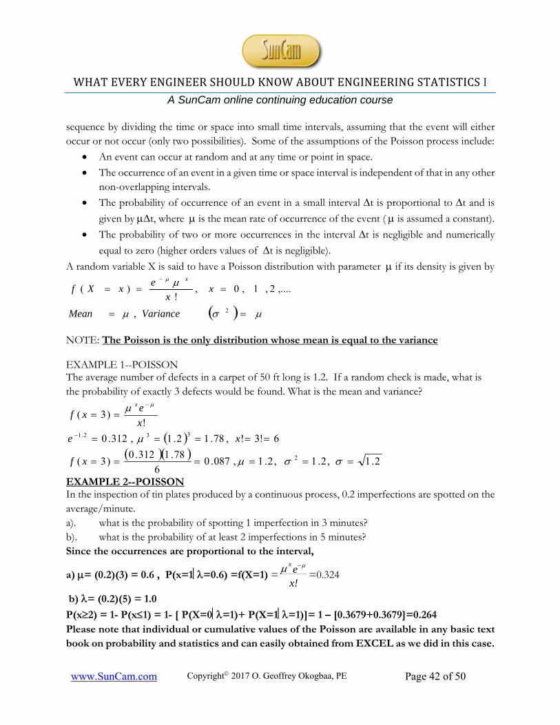
WHAT EVERY ENGINEER SHOULD KNOW ABOUT ENGINEERING STATISTICS I
A SunCam online continuing education course
www.SunCam.com Copyright 2017 O. Geoffrey Okogbaa, PE Page 42 of 50
sequence by dividing the time or space into small time intervals, assuming that the event will either occur or not occur (only two possibilities). Some of the assumptions of the Poisson process include:
An event can occur at random and at any time or point in space.
The occurrence of an event in a given time or space interval is independent of that in any other non-overlapping intervals.
The probability of occurrence of an event in a small interval t is proportional to t and is
given by t, where is the mean rate of occurrence of the event ( is assumed a constant).
The probability of two or more occurrences in the interval t is negligible and numerically
equal to zero (higher orders values of t is negligible).
A random variable X is said to have a Poisson distribution with parameter if its density is given by
2,
,....2,1,0,!
)(
VarianceMean
xx
exXf
x
NOTE: The Poisson is the only distribution whose mean is equal to the variance EXAMPLE 1--POISSON The average number of defects in a carpet of 50 ft long is 1.2. If a random check is made, what is the probability of exactly 3 defects would be found. What is the mean and variance?
2.1,2.1,2.1,087.06
78.1312.0)3(
6!3!,78.12.1,312.0
!)3(
2
332.1
xf
xe
x
exf
x
EXAMPLE 2--POISSON In the inspection of tin plates produced by a continuous process, 0.2 imperfections are spotted on the average/minute. a). what is the probability of spotting 1 imperfection in 3 minutes? b). what is the probability of at least 2 imperfections in 5 minutes? Since the occurrences are proportional to the interval,
a) = (0.2)(3) = 0.6 , P(x=1=0.6) =f(X=1) =x!e
x
=0.324
b) = (0.2)(5) = 1.0
P(x2) = 1- P(x1) = 1- [ P(X=0=1)+ P(X=1=1)]= 1 – [0.3679+0.3679]=0.264 Please note that individual or cumulative values of the Poisson are available in any basic text book on probability and statistics and can easily obtained from EXCEL as we did in this case.
WHAT EVERY ENGINEER SHOULD KNOW ABOUT ENGINEERING STATISTICS I
A SunCam online continuing education course
www.SunCam.com Copyright 2017 O. Geoffrey Okogbaa, PE Page 43 of 50
From the Poisson such a table
(a) P(x=1;), =(t)= (0.2)(3) = 0.6 , P(x=1) = F(1,0.6) - F(0,0.6) = 0.878 -0.549 = 0.324 (b) P(x=1) =(t)= (0.2)(5) = 1.0 P(x2) = 1- P(x) = 1- F(1,1)= 1 - 0.736 =0.264 ContinuousRandomVariables Let X be a random variable. Suppose that the range space of X consists of intervals rather than points (there are infinite numbers of points in the interval), then X is a continuous random variable– X may assume all values in the interval
Continuous Random variables are those that assume i) Any value on the interval on the real line R. For example, the weight of a container in a
filling operation ii) Any value in a half infinite interval on the real line (the strength of a component may
take values in the interval (0, infinity]. Let X be a random variable. The probability density function of X denoted by pdf is a function f satisfying the following: a). f(x) ≥ 0 for all X, XεRx , (b).
dxxxf )( , 222 )(
dxxfx
Example of the analyses of a general continuous random variable
Find a). The constant k b). Compute P(0.1 < x < 0.2), c). Compute P(x >0.5) d). Find the cumulative function F(x) and show the limits or boundaries e) Find the mean µ and the variance 2
Note for this data, the limits are (0,1], so: 1
0
)( dxxxf 21
0
22 )( dxxfx
11 32
0 0
0.20.2 32
0.1 0.1
0.50.5 32
0 0
1 3). (1 ) 1 1 1 1,
3 3 2
3 3). (0.1 0.2) (1 ) 0.15 0.0035 0.1465
2 2 3
3 3 5). ( 0.5) 1 ( 0.5) 1 (1 ) , 1
2 2 3 16
xa k x k x k k
xb P x x dx x
xc P x P x x dx x
1)( XR
xf
1)(,
xfgeneralIn
elsewhere
xxkxfGiven 0
10)1()(:
2
WHAT EVERY ENGINEER SHOULD KNOW ABOUT ENGINEERING STATISTICS I
A SunCam online continuing education course
www.SunCam.com Copyright 2017 O. Geoffrey Okogbaa, PE Page 44 of 50
3
2
3
). ( ) ( )
3 3( ) ( ) 1
2 2 3
0, ( ) 0
1, ( ) 1 1 1 0
0 0
3( ) 0 1
2
1 1
x
d F x f t dt
xF x f x dx x dx x C
for x F x
x F x C C
x
x xF x x
x
11 1 2 42
0 0 0
12 2 2
0
11 1 3 52 2 2
0 0 0
22
3 3 3 1 1 3) 1
2 2 2 4 2 2 4 8
3 3 3 1 1 3 2 11
2 2 3 5 2 3 5 2 15 5
1 3 1 9 64 45 19 1,
5 8 5 64 320 320
x xe xf x dx x x dx
x f x dx
x xx f x dx x x dx
9
320
11.1 CommonContinuousDistributions Among the continuous distributions that we will examine include: normal, the Uniform and the exponential. For each of these distributions we will provide details and examples that would make it easy for an engineer to identify them based on certain behaviors or characteristics that are observed in the process under study
11.1.1TheNormalDistribution All normal distributions are symmetric and have bell-shaped density curves with a single peak. To speak specifically of any normal distribution, two quantities have to be specified: the mean, where the peak of the density occurs, and the standard deviation, which indicates the spread or girth of the bell curve. Normal distributions are symmetric, unimodal and the mean, median, and mode are all equal. A normal distribution is perfectly symmetrical around its center. That is, the right side of the center is a mirror image of the left side. Some of the major characteristics include:
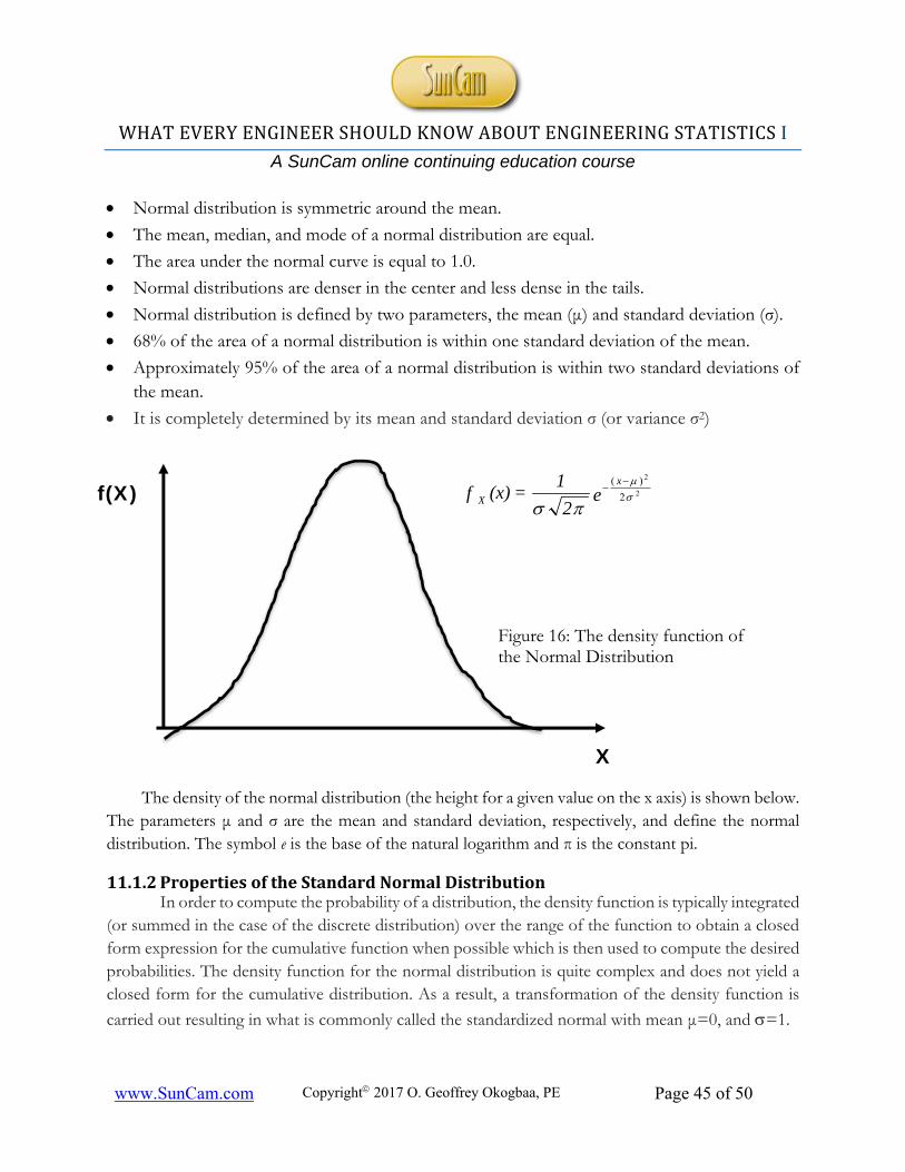
WHAT EVERY ENGINEER SHOULD KNOW ABOUT ENGINEERING STATISTICS I
A SunCam online continuing education course
www.SunCam.com Copyright 2017 O. Geoffrey Okogbaa, PE Page 45 of 50
Normal distribution is symmetric around the mean.
The mean, median, and mode of a normal distribution are equal.
The area under the normal curve is equal to 1.0.
Normal distributions are denser in the center and less dense in the tails.
Normal distribution is defined by two parameters, the mean (μ) and standard deviation (σ).
68% of the area of a normal distribution is within one standard deviation of the mean.
Approximately 95% of the area of a normal distribution is within two standard deviations of the mean.
It is completely determined by its mean and standard deviation σ (or variance σ2)
The density of the normal distribution (the height for a given value on the x axis) is shown below.
The parameters μ and σ are the mean and standard deviation, respectively, and define the normal distribution. The symbol e is the base of the natural logarithm and π is the constant pi.
11.1.2PropertiesoftheStandardNormalDistribution In order to compute the probability of a distribution, the density function is typically integrated (or summed in the case of the discrete distribution) over the range of the function to obtain a closed form expression for the cumulative function when possible which is then used to compute the desired probabilities. The density function for the normal distribution is quite complex and does not yield a closed form for the cumulative distribution. As a result, a transformation of the density function is
carried out resulting in what is commonly called the standardized normal with mean μ=0, and =1.
X
f(X)
Figure 16: The density function of the Normal Distribution
e2
1 = (x)f
x
X2
2
2
)(
WHAT EVERY ENGINEER SHOULD KNOW ABOUT ENGINEERING STATISTICS I
A SunCam online continuing education course
www.SunCam.com Copyright 2017 O. Geoffrey Okogbaa, PE Page 46 of 50
A new variable Z (defined as the number of standard deviations from the mean or the standard
deviate) results with values from - to + and the probability is evaluated based on the number of standard deviates away from the mean. Thus, the probability (or area) corresponding to a give number of standard deviation Z is give as Ф(Z). Due to symmetry, Ф(Z)=1- Ф(-Z).
by definition and due to the transformation
X
Z . Give Z (also called the Z- score) then one
can use the standard normal table determine the desired probabilities or areas. Tables of the standard normal are available in most statistics and probability texts. For the standard normal, the probability of the normal random variable X taking on a value less than x0 is cumulative distribution function is
defined as P(X<x 0 ) = z , where Z =[ ( x0 - μ)/] is the number of standard deviations between the mean and x0 . Note the following important relationship. Ф(Z)=1- Ф(-Z) Ф(1.28) =0.9 or 90%, Ф(-1.28)=0.1 or 10% Z0.1 = -Z0.9
Normal Distribution Examples Example 1.
Assume life in hours of a tube is normally distributed with N(200, 2). A purchaser requires at least
90% of the tubes to have lives exceeding 150 hr. What is the maximum value of under this condition.
Ф(-1.28) = 0.1 in the left tail (150<200). Z= -1.28, = 39.1
Since Z = (x-μ)/
-1.28 = (150-200)/ -1.28 = -50/ =50/1.28=39.1 Example 2. A manufacturer knows that the process for the diameters of the pistons he manufactures follows a
normal distribution with mean of 2.5 cm and standard deviation of 0.025 cm. If a customer has specification limits of 2.45 cm and 2.54 cm, what percentage of the manufacturers pistons will not meet the customer's specs.?
P(2.45 < x < 2.51) = P[ (2.45-2.5) / 0.025 < z < (2.51- 2.5) / 0.025 ] P(-2 < z < 2.4 ) = P( z < 2.4) - P( z < -2.0) = Ф (2.4) - Ф(-2.0) = 0.97932 - (1-0.97725), [ Note: Ф ( - z) = 1- Ф( z) if z > 0 ]. = 0.97932 - 0.02275 (From the Standard Normal Table in EXCEL) = 0.95657.
The proportion of pistons that would fall within the customer’s specs =95.6% Therefore, the percentage that would fall outside of specs is 100(1-0.95657) = 4.4%
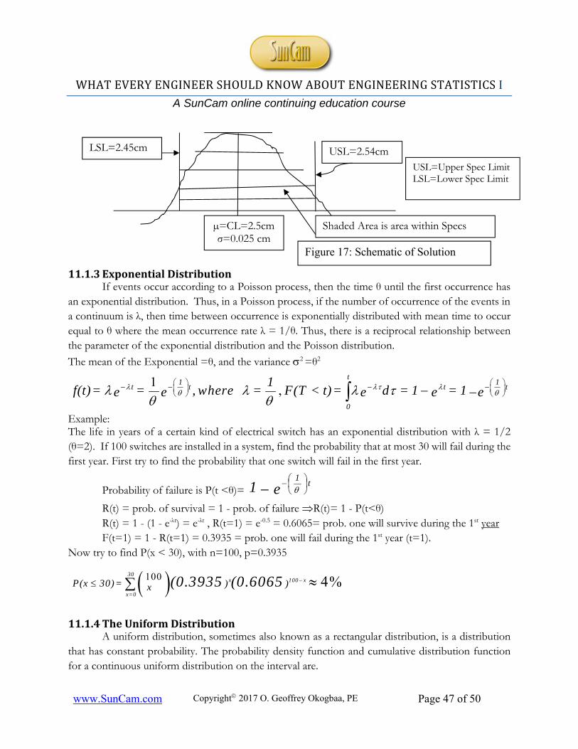
WHAT EVERY ENGINEER SHOULD KNOW ABOUT ENGINEERING STATISTICS I
A SunCam online continuing education course
www.SunCam.com Copyright 2017 O. Geoffrey Okogbaa, PE Page 47 of 50
11.1.3ExponentialDistribution If events occur according to a Poisson process, then the time θ until the first occurrence has an exponential distribution. Thus, in a Poisson process, if the number of occurrence of the events in a continuum is λ, then time between occurrence is exponentially distributed with mean time to occur equal to θ where the mean occurrence rate λ = 1/θ. Thus, there is a reciprocal relationship between the parameter of the exponential distribution and the Poisson distribution.
The mean of the Exponential =θ, and the variance 2 =θ2
1,
t1 1
t t t t
0
1f(t) = = , where = F(T < t) = d = 1 = 1 e e e e e
Example: The life in years of a certain kind of electrical switch has an exponential distribution with λ = 1/2 (θ=2). If 100 switches are installed in a system, find the probability that at most 30 will fail during the first year. First try to find the probability that one switch will fail in the first year.
Probability of failure is P(t <θ)= e 1 t1
R(t) = prob. of survival = 1 - prob. of failure R(t)= 1 - P(t<θ) R(t) = 1 - (1 - e-λt) = e-λt , R(t=1) = e-0.5 = 0.6065= prob. one will survive during the 1st year F(t=1) = 1 - R(t=1) = 0.3935 = prob. one will fail during the 1st year (t=1).
Now try to find P(x < 30), with n=100, p=0.3935
11.1.4TheUniformDistribution A uniform distribution, sometimes also known as a rectangular distribution, is a distribution that has constant probability. The probability density function and cumulative distribution function for a continuous uniform distribution on the interval are.
100 4%30
x 100 x
x=0
P(x 30) = ) )x (0.3935 (0.6065
USL=2.54cm LSL=2.45cm
µ=CL=2.5cm σ=0.025 cm
Shaded Area is area within Specs
USL=Upper Spec Limit LSL=Lower Spec Limit
Figure 17: Schematic of Solution
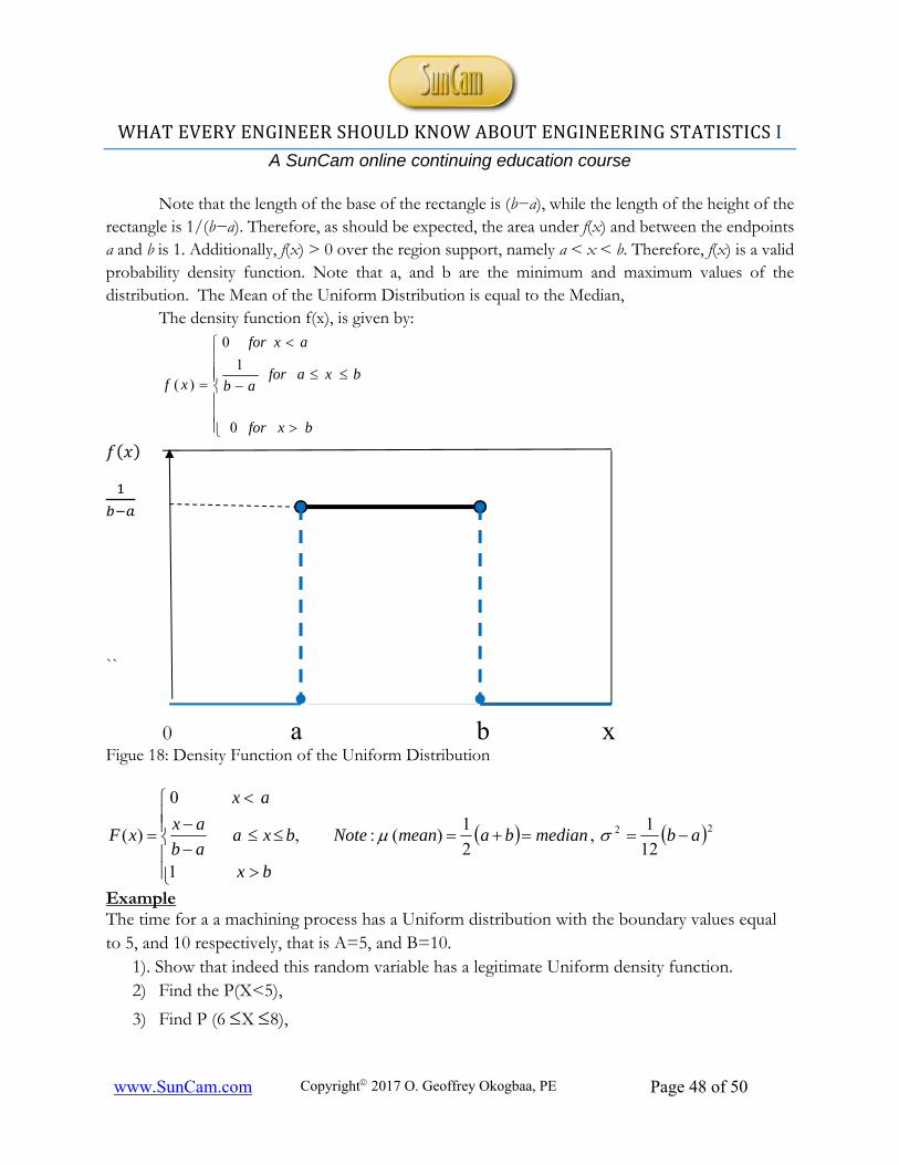
WHAT EVERY ENGINEER SHOULD KNOW ABOUT ENGINEERING STATISTICS I
A SunCam online continuing education course
www.SunCam.com Copyright 2017 O. Geoffrey Okogbaa, PE Page 48 of 50
Note that the length of the base of the rectangle is (b−a), while the length of the height of the rectangle is 1/(b−a). Therefore, as should be expected, the area under f(x) and between the endpoints a and b is 1. Additionally, f(x) > 0 over the region support, namely a < x < b. Therefore, f(x) is a valid probability density function. Note that a, and b are the minimum and maximum values of the distribution. The Mean of the Uniform Distribution is equal to the Median, The density function f(x), is given by:
bxfor
bxaforab
axfor
xf
0
1
0
)(
𝑓 𝑥
``
0 a b x Figue 18: Density Function of the Uniform Distribution
22
12
1,
2
1)(:,
1
0
)( abmedianbameanNote
bx
bxaab
ax
ax
xF
Example The time for a a machining process has a Uniform distribution with the boundary values equal to 5, and 10 respectively, that is A=5, and B=10.
1). Show that indeed this random variable has a legitimate Uniform density function. 2) Find the P(X<5),
3) Find P (6 X 8),
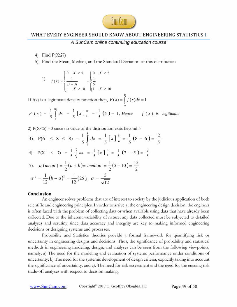
WHAT EVERY ENGINEER SHOULD KNOW ABOUT ENGINEERING STATISTICS I
A SunCam online continuing education course
www.SunCam.com Copyright 2017 O. Geoffrey Okogbaa, PE Page 49 of 50
4) Find P(X7) 5) Find the Mean, Median, and the Standard Deviation of this distribution
1).
1015
1
50
101
1
50
)(
X
X
XAB
X
xf
If f(x) is a legitimate density function then, B
A
dxxfxF 1)()(
legitimateisxfHencexdxxF )(,155
1
5
1
5
1)(
10
5
10
5
2) P(X<5) =0 since no value of the distribution exits beyond 5
5
268
5
1
5
1
5
1 =8) X P(63).
8
6
8
6
xdx
5
257
5
1
5
1
5
1 =7) P(X4).
5
5
7
5
xdx
12
5,25
12
1
12
12
15105
2
1
2
1)().5
22
ab
medianbamean
Conclusion
An engineer solves problems that are of interest to society by the judicious application of both scientific and engineering principles. In order to arrive at the engineering design decision, the engineer is often faced with the problem of collecting data or when available using data that have already been collected. Due to the inherent variability of nature, any data collected must be subjected to detailed analyses and scrutiny since data accuracy and integrity are key to making informed engineering decisions or designing systems and processes.
Probability and Statistics theories provide a formal framework for quantifying risk or uncertainty in engineering designs and decisions. Thus, the significance of probability and statistical methods in engineering modeling, design, and analyses can be seen from the following viewpoints, namely; a) The need for the modeling and evaluation of systems performance under conditions of uncertainty; b) The need for the systemic development of design criteria, explicitly taking into account the significance of uncertainty, and c). The need for risk assessment and the need for the ensuing risk trade-off analyses with respect to decision making.
WHAT EVERY ENGINEER SHOULD KNOW ABOUT ENGINEERING STATISTICS I
A SunCam online continuing education course
www.SunCam.com Copyright 2017 O. Geoffrey Okogbaa, PE Page 50 of 50
The reviews and materials presented herein are an attempt to give the engineer a very broad overview of the concepts of Probability and Statistics. Some details have been omitted especially if those do not contribute essentially to the understanding of the concepts. For example, tables for some of the well-known distributions have been left out because they are available online or in any basic Probability and Stat book. Numerical problems have been provided to help elucidate some of the concepts. REFERENCES1. Ang, A.H.-S. and Tang, W.H. (1975). Probability Concepts in Engineering Planning and Design,
Vol. 1, Basic Principles, John Wiley, New York. 2. Kelly Brown, 'A Terabyte of Storage Space: How Much is Too Much,' in The Information Umbrella,
Musings on Applied Information Management, University of Oregon, 2014. 3. “Data to Action,” A Harvard Business Review (HBR) Insight Center White Paper, Sponsored by
SAS, Inc., 2014, Harvard Business Publishing, Cambridge, M. 4. “Big Data Analytics, What it is and why it matters,” International Institute for Analytics, Thomas H.
Davenport and Jill Dyché, Copyright © Thomas H. Davenport and SAS, Institute Inc, 2013. 5. International Federation of Robotics (IFR), Executive Summary, World Robotics 2013-2015. 6. Nuclear Power Plants World-wide, Source European Nuclear Society, November 2016. 7. Johnson, R.., Miller, I. (2015), Miller & Freund's Probability & Statistics, 9th ed., Pearson Publishers,
Boston, MA, USA. 8. Vardeman, S. (1994), Statistics for Engineering problem solving, 1st ed., PWS Pub. Co, Boston, MA. 9. Montgomery, D.C., Runger, G., and Hubele, N. (1998), Engineering Statistics, 1st ed, John Wiley and
Sons, NY, USA. 10. Montgomery, D.C., and Runger, G. (2011), Applied Statistics and Probability for Engineers, 5th ed.,
John Wiley and Sons, NY. 11. Devore, J.L., (2012), Probability and Statistics for Engineering and the Sciences, 8th ed., Duxbury & Brooks/Cole, Boston, MA. 12. Ross, S. (1987), Introduction to Probability and Statistics for Engineers and Scientists, 1st ed., John
Wiley & Sons, NY. 13. Walpole, R., Meyers, R.H. (2002), Probability and Statistics for Engineers and Scientists, 7th ed.,
Prentice- Hall Inc., Upper Saddle River, NJ. 14. Hogg, R. Craig, A. (2004), Introduction to Mathematical Statistics, 6th ed., Prentice-Hall, Englewood Cliffs, NJ. 15. Larsen R.J., Marx M.L. (2012), Introduction to Mathematical Statistics and Its Applications, 5th ed.,
Prentice-Hall Englewood Cliffs, NJ. 16. DeGroot M.H., Schervish M.J. (2011), Probability and Statistics,4th ed., Addison Wesley, Boston, MA