o Electron Spin Resonance - Henri Menke Electron Spin Resonance Michael Schmid and Henri Menkey Gruppe M05, Fortgeschrittenenpraktikum, University of Stuttgart (November 10, 2014)

FP V24 (2015) FORTGESCHRITTENENPRAKTIKUM November 10, 2014

o

Electron Spin Resonance

Michael Schmid∗ and Henri Menke†

Gruppe M05, Fortgeschrittenenpraktikum, University of Stuttgart(November 10, 2014)

The present experiment is mainly divided in two parts. At first we want to characterise the modesof a reflex klystron, record the characteristic curve of the detector diode and measure the standingwave ratio for different experimental adaptations. Second we calibrate the magnetic field of theexperimental implementation of the electron spin resonance (ESR). Thereafter we investigate theESR spectrum of different probes and the hyperfine structure of Mn2+ and DPPH. Especially wewant to determine the Lande g-factors of Cu2+ and Mn2+ and analyse the spin-exchange in TEMPOsolutions.

BASICS

To understand why we need microwaves in this exper-iment let us look at the level splitting of an electron.The splitting energy is given by ∆E = geµBBres and isequivalent to the applied electromagnetic wave hν. Itfollows that ν = geµBBres/h which is roughly 9 GHz forreasonable fields of about 300 mT.

Microwaves

Electromagnetic waves in the range from 1 GHz to300 GHz (corresponding to a wavelength of 30 cm to 1 mm)are called microwaves. In everyday life microwaves arepresent in mobile communication such as WiFi, operatingat 2.4 GHz and 5 GHz (since 2013), and radar engineering.Before we discuss the generation of microwaves we repeatsome basics of electrodynamics to better understand prop-agation and refraction of microwaves.

Maxwell’s Equations

To describe electromagnetic waves in vacuum it is nec-essary to know the fundamental equations of electrody-namics

∇ ·B = 0 (1)

∇ ·E =%

ε0(2)

∇×E = −∂tB (3)

∇×B = µ0j + µ0ε0∂tE (4)

the Maxwell equations. Here B (E) is the magnetic(electric) field, % the charge density, j the current density,ε0 the permittivity of free space, and µ0 the permeabilityof free space. Equation (1) allows to find a vector potentialA that fulfils B = ∇×A (see vector calculus). With helpof equation (3) and the vector potential we can ensure theexistence of a scalar potential φ with −∇φ = E + ∂tA.

With help of the Lorenz gauge condition

∇ ·A− ε0µ0∂tφ = 0 (5)

and the help of equation (4) it is possible to identify waveequations for the potentials(

∆− 1

c2∂2t

)φ =

√µ0

ε0%, (6)(

∆− 1

c2∂2t

)A = µ0j. (7)

Using the D’Alembert operator and the covariant for-mulation of electrodynamics allows to find a much morebeautiful form of Maxwell’s equations, namely

∂µ∂µAν = µ0j

ν , (8)

where Aµ = (φ/c,A) and jµ = (c%, j) are four-vectors.It is an easy exercise to determine the wave equation

for E in vacuum

�E = 0. (9)

The solution for electric waves in vacuum are plane waves

E(r, t) = E0ei(k·r−ωt) (10)

with der dispersion relation ω = c|k|. If we want to solveMaxwell’s equation in waveguides we have to observeadditional boundary conditions.

Generation of Microwaves

To generate electromagnetic waves of any kind in acontrolled way a cavity is needed. A cavity has the advan-tage that we can precisely control which modes of a wavewe get. Furthermore, a switch between continuous waveand pulsed wave can be achieved using a cavity. Herewe will only use continuous wave, though. There a twokinds of cavities for the generation of microwaves whichare presented in the following: The two chamber klystronand the reflex klystron.

1


(a)

KA

l

H2H1

U0

− +

(b)

KR

H

− −+ +

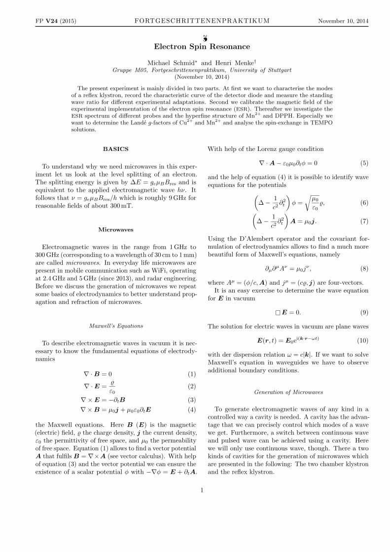
FIG. 1. (a) Sketch of a two chamber klystron, taken from [1,p. 479]. Electrons are generated at the cathode K and accel-erated by a positively charged slit. The resonator H1 appliesa velocity modulation, resonator H2 a density modulation.The backcoupling of both allows usage as cavity. (b) Sketchof a reflex klystron, also taken from [1, p. 479]. Electronsare again generated at the cathode K and accelerated by aslit but then reflected by the repeller R. This results in areversal of the direction of flight and, if the repeller voltagewas chosen appropriately, in a resonant mode in the cavity. Inthis experiment we use a reflex klystron.

Two Chamber Klystron: A sketch of a two chamberklystron can be viewed in figure 1 a). A hot cathode emitselectrons that are accelerated by a positively charged slitto energies in the range of several keV. The electron beamenters the first chamber H1. The electric field present inH1 accelerated or slows down the electrons depending ontheir velocity. This velocity modulation leads to formationof clusters with electrons of the same speed, which can beviewed as a density modulation. The second chamber isplaced at the maximum of the density amplitude wherethis oscillation produces a voltage in the walls of the

chamber with the same frequency as the mode in the firstchamber. The frequency depends on the geometry of theresonator and can thus not be influenced easily.

Reflex Klystron: A sketch of a reflex klystron is de-picted in figure 1 b). A reflex klystron only consists ofone resonator. Instead of the second resonator there is areflector electrode, which is negatively charged. Duringthe slowing down and accelerating in the opposite direc-tion a density modulation emerges. During the secondpass through the resonator the electrons exchange energywith the resonator mode. Only if the electrons have thecorrect velocity on reentering of the cavity (determinedby UR) they provide energy to the field by slowing down,else they absorb energy from the field to accelerate.

Microwaves in waveguides

Every linear structure that conveys electromagneticwaves is called waveguide. The waveguides used in theexperiment are hollow metal pipes. With the help ofMaxwell’s equations and boundary conditions determinedby the properties of the materials it is possible to analysethe behaviour of microwaves in waveguides and identifythe possible modes. Henceforth the waveguide is assumedto be aligned in z-direction. Electromagnetic waves prop-agating in waveguides are reflected on the walls and formstanding waves leading to a discrete spectrum of allowedmodes.

To identify the possible modes it is necessary to solvethe wave equation (9). Due to the alignment of thewaveguide we use the ansatz

E(r, t) = E0(x, y) cos(ωt− kzz) (11)

which yields

∂2xE + ∂2

yE +( ωc2− k2

z

)E = 0. (12)

The boundary conditions in waveguides demand a vanish-ing tangential component ofE on the walls (von Neumanncondition). This implies that the electric field E is alwaysperpendicular to the magnetic field B which is there-fore orientated tangentially to the conductive walls. Thisconditions are fulfilled if

kx =πn

a, ky =

πm

b(13)

and n,m ∈ N. The constants a and b describe the widthand height of the waveguide. Using Maxwell’s equationswe identify:

TE-Modes: Solutions that have no electric field in thedirection of propagation (E ⊥ ez) are called transverseelectric modes.

TM-Modes: Solutions that have no magnetic field inthe direction of propagation (B ⊥ ez) are called trans-verse magnetic modes.

2


TEM-Modes: Transverse electromagnetic modes haveneither an electric field nor a magnetic field component inthe direction of propagation. Due to Maxwell’s equationsthese solutions are not possible in hollow waveguides.However TEM-modes can propagate in coaxial cables orfree space.

To investigate the dispersion in hollow waveguides weuse ω = ck and the conditions (13)

kz =

√ω2

c2− π

(n2

a2+m2

b2

)=√k2 − k2

g . (14)

An undamped propagation in z-direction is only possibleif the threshold wavelength λg = 2π/kg is greater thanthe wavelength of the electromagnetic wave λ or kg ≥ k.The threshold wavelength is therefore given by

λg = 2

(n2

a2+m2

b2

)−1/2

. (15)

To compare the vacuum wavelength λv = c/ν with λgit is common to define an effective wavelength

λe ≡2π

kz= λv

(1− λ2

v

λ2g

)−1/2

. (16)

Obviously the wavelength of electromagnetic waves inhollow waveguides is greater than the wavelength of anelectromagnetic waves of the same frequency in vacuum.

Standing Waves: A standing wave is caused by the in-terference of two waves propagating in opposite directions(e.g. interference between an incoming and a reflectedwave). The two waves are described by

Ei(r, t) = E0 cos(ωt− kz) (17)

Er(r, t) = E0 cos(ωt+ kz). (18)

The interference of both waves is

E(r, t) = Ei(r, t) +Er(r, t)

= 2E0 sin(kz) cos(ωt) (19)

where we used some trigonometric identities. This func-tion of a standing wave is characterised by its nodes andantinodes. The gifted reader might have noticed that forstanding waves it is not possible to transport energy andtherefore they are impractical for our experiment.

Reflection of Waves

When a wave hits the end of a waveguide, whateverboundary condition applies, it is reflected. This is not ahard reflection where 100 % of the wave are scattered back-wards, but a transition from a regime of a first impedance

Z1 into a regime of another impedance Z2. In general theimpedance depends on the position inside the waveguide,i.e., Z = Z(r). For the vacuum we find Zvac =

√µ0/ε0.

For the transition Z1 → Z2 we find the reflection coeffi-cient

p =E(r)

E(i)=Z2 − Z1

Z2 + Z1

The indices (r) und (i) stand for fur reflected and incident,respectively. The reflection coefficient is p = 0 if Z2 = Z1.Therefore open end waveguides are capped by a terminalresistance. To keep the reflection factor small one triesto smoothly transfer waves from one guide to another, inthe case of microwaves using so called horn radiators.

Reflected waves inside a waveguide lead to (undesired)standing waves, as discussed above. Those standing wavesare in most cases not completely stationary, but are su-perimposed with propagating parts. To quantify theamount of superposition one defines the standing wave ra-tio (SWR) as the ratio of maximum and minimum electricfield amplitude

SWR ≡ Emax

Emin=|E(i)

1 |+ |E(r)1 |

|E(i)1 | − |E

(r)1 |

=1 + |p|1− |p|

(20)

with the just introduced reflection coefficient p. There aretwo limit cases worth mentioning: SWR = 1 ⇐⇒ |p| = 0corresponds to an ideal setup as there is no reflectionat all, whereas SWR = ∞ ⇐⇒ |p| = 1 resembles theworst case of total reflection, i.e. standing waves insidethe waveguide.

Determining the SWR

There are three different techniques to determine theSWR in a hollow waveguide, which are all presented inthe following. All of the are based on the insertion of aprobe into the waveguide.

Interlude on Damping: To quantify ratios using theDecibel scale one computes the logarithm of the ratioto base ten and multiplies the result with ten. Hence,10 dB corresponds to a tenfold increase, whereas 3 dBapproximately describes a doubling and 3 dB a halving.Formally one has

L(E1, E2) = 10 log10

(E2

1

E22

)dB

= 20 log10

(E1

E2

)dB

= 2 log10

(E1

E2

)B

Because the damping takes place over the whole extent ofthe waveguide, it is common to put it in relation to that.In most cases this is dB/10 m or dB/100 m.

3


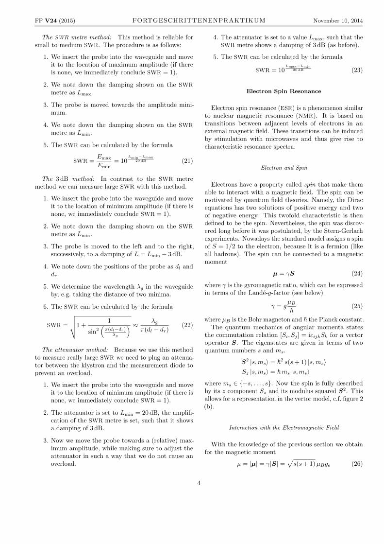
The SWR metre method: This method is reliable forsmall to medium SWR. The procedure is as follows:

1. We insert the probe into the waveguide and moveit to the location of maximum amplitude (if thereis none, we immediately conclude SWR = 1).

2. We note down the damping shown on the SWR

metre as Lmax.

3. The probe is moved towards the amplitude mini-mum.


metre as Lmin.

5. The SWR can be calculated by the formula

SWR =Emax

Emin= 10

Lmin−Lmax20 dB (21)

The 3 dB method: In contrast to the SWR metremethod we can measure large SWR with this method.

1. We insert the probe into the waveguide and moveit to the location of minimum amplitude (if there isnone, we immediately conclude SWR = 1).


metre as Lmin.

3. The probe is moved to the left and to the right,successively, to a damping of L = Lmin − 3 dB.

4. We note down the positions of the probe as dl anddr.

5. We determine the wavelength λg in the waveguideby, e.g. taking the distance of two minima.


SWR =

√√√√1 +1

sin2(π(dl−dr)

λg

) ≈ λgπ(dl − dr)

(22)

The attenuator method: Because we use this methodto measure really large SWR we need to plug an attenua-tor between the klystron and the measurement diode toprevent an overload.

1. We insert the probe into the waveguide and moveit to the location of minimum amplitude (if there isnone, we immediately conclude SWR = 1).

2. The attenuator is set to Lmin = 20 dB, the amplifi-cation of the SWR metre is set, such that it showsa damping of 3 dB.

3. Now we move the probe towards a (relative) max-imum amplitude, while making sure to adjust theattenuator in such a way that we do not cause anoverload.

4. The attenuator is set to a value Lmax, such that theSWR metre shows a damping of 3 dB (as before).


SWR = 10Lmax−Lmin

20 dB (23)

Electron Spin Resonance

Electron spin resonance (ESR) is a phenomenon similarto nuclear magnetic resonance (NMR). It is based ontransitions between adjacent levels of electrons in anexternal magnetic field. These transitions can be inducedby stimulation with microwaves and thus give rise tocharacteristic resonance spectra.

Electron and Spin

Electrons have a property called spin that make themable to interact with a magnetic field. The spin can bemotivated by quantum field theories. Namely, the Diracequations has two solutions of positive energy and twoof negative energy. This twofold characteristic is thendefined to be the spin. Nevertheless, the spin was discov-ered long before it was postulated, by the Stern-Gerlachexperiments. Nowadays the standard model assigns a spinof S = 1/2 to the electron, because it is a fermion (likeall hadrons). The spin can be connected to a magneticmoment

µ = γS (24)

where γ is the gyromagnetic ratio, which can be expressedin terms of the Lande-g-factor (see below)

γ = gµB~

(25)

where µB is the Bohr magneton and ~ the Planck constant.The quantum mechanics of angular momenta states

the commutation relation [Si, Sj ] = iεijkSk for a vectoroperator S. The eigenstates are given in terms of twoquantum numbers s and ms.

S2 |s,ms〉 = ~2 s(s+ 1) |s,ms〉Sz |s,ms〉 = ~ms |s,ms〉

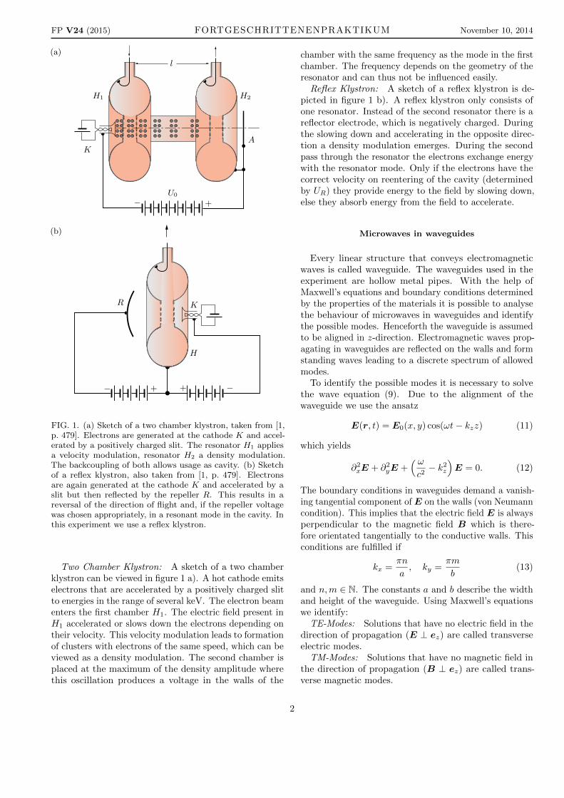
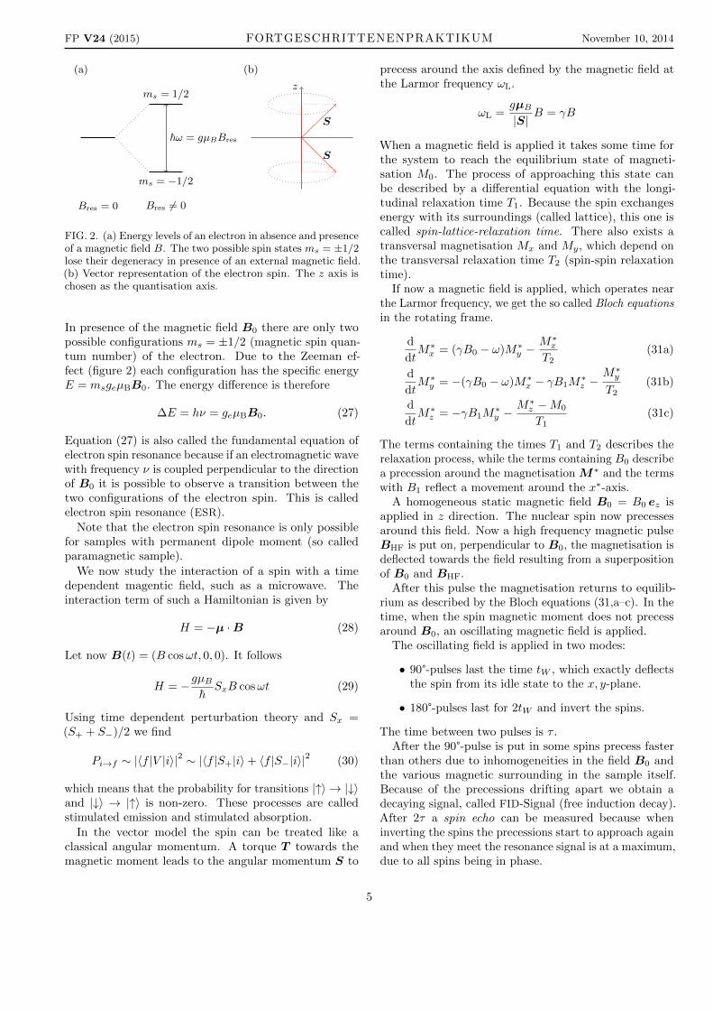
where ms ∈ {−s, . . . , s}. Now the spin is fully describedby its z component Sz and its modulus squared S2. Thisallows for a representation in the vector model, c.f. figure 2(b).

Interaction with the Electromagnetic Field

With the knowledge of the previous section we obtainfor the magnetic moment

µ = |µ| = γ|S| =√s(s+ 1)µBge (26)

4


(a)

Bres = 0 Bres 6= 0

ms = 1/2

ms = −1/2

~ω = gµBBres

(b)

z

S

S

FIG. 2. (a) Energy levels of an electron in absence and presenceof a magnetic field B. The two possible spin states ms = ±1/2lose their degeneracy in presence of an external magnetic field.(b) Vector representation of the electron spin. The z axis ischosen as the quantisation axis.

In presence of the magnetic field B0 there are only twopossible configurations ms = ±1/2 (magnetic spin quan-tum number) of the electron. Due to the Zeeman ef-fect (figure 2) each configuration has the specific energyE = msgeµBB0. The energy difference is therefore

∆E = hν = geµBB0. (27)

Equation (27) is also called the fundamental equation ofelectron spin resonance because if an electromagnetic wavewith frequency ν is coupled perpendicular to the directionof B0 it is possible to observe a transition between thetwo configurations of the electron spin. This is calledelectron spin resonance (ESR).

Note that the electron spin resonance is only possiblefor samples with permanent dipole moment (so calledparamagnetic sample).

We now study the interaction of a spin with a timedependent magentic field, such as a microwave. Theinteraction term of such a Hamiltonian is given by

H = −µ ·B (28)

Let now B(t) = (B cosωt, 0, 0). It follows

H = −gµB~SxB cosωt (29)

Using time dependent perturbation theory and Sx =(S+ + S−)/2 we find

Pi→f ∼ |〈f |V |i〉|2 ∼ |〈f |S+|i〉+ 〈f |S−|i〉|2 (30)

which means that the probability for transitions |↑〉 → |↓〉and |↓〉 → |↑〉 is non-zero. These processes are calledstimulated emission and stimulated absorption.

In the vector model the spin can be treated like aclassical angular momentum. A torque T towards themagnetic moment leads to the angular momentum S to

precess around the axis defined by the magnetic field atthe Larmor frequency ωL.

ωL =gµB|S|

B = γB

When a magnetic field is applied it takes some time forthe system to reach the equilibrium state of magneti-sation M0. The process of approaching this state canbe described by a differential equation with the longi-tudinal relaxation time T1. Because the spin exchangesenergy with its surroundings (called lattice), this one iscalled spin-lattice-relaxation time. There also exists atransversal magnetisation Mx and My, which depend onthe transversal relaxation time T2 (spin-spin relaxationtime).

If now a magnetic field is applied, which operates nearthe Larmor frequency, we get the so called Bloch equationsin the rotating frame.

d

dtM∗x = (γB0 − ω)M∗y −

M∗xT2

(31a)

d

dtM∗y = −(γB0 − ω)M∗x − γB1M

∗z −

M∗yT2

(31b)

d

dtM∗z = −γB1M

∗y −

M∗z −M0

T1(31c)

The terms containing the times T1 and T2 describes therelaxation process, while the terms containing B0 describea precession around the magnetisation M∗ and the termswith B1 reflect a movement around the x∗-axis.

A homogeneous static magnetic field B0 = B0 ez isapplied in z direction. The nuclear spin now precessesaround this field. Now a high frequency magnetic pulseBHF is put on, perpendicular to B0, the magnetisation isdeflected towards the field resulting from a superpositionof B0 and BHF.

After this pulse the magnetisation returns to equilib-rium as described by the Bloch equations (31,a–c). In thetime, when the spin magnetic moment does not precessaround B0, an oscillating magnetic field is applied.

The oscillating field is applied in two modes:

• 90°-pulses last the time tW , which exactly deflectsthe spin from its idle state to the x, y-plane.

• 180°-pulses last for 2tW and invert the spins.

The time between two pulses is τ .After the 90°-pulse is put in some spins precess faster

than others due to inhomogeneities in the field B0 andthe various magnetic surrounding in the sample itself.Because of the precessions drifting apart we obtain adecaying signal, called FID-Signal (free induction decay).After 2τ a spin echo can be measured because wheninverting the spins the precessions start to approach againand when they meet the resonance signal is at a maximum,due to all spins being in phase.

5


The Lande g-factor

In general the Lande g-factor isn’t a simple scalar.This is only true for free electrons. Because the g-factoris anisotropic in many crystals it is necessary to introducea symmetric Tensor g which is diagonalisable and has theform

g =

gxx 0 00 gyy 00 0 gzz

. (32)

The directions parallel to the eigenvectors of the eigenbasisare called principal axes.

In many physical problems the g Tensor has an addi-tional symmetry that allows gxx = gyy. Consequently weare able to define two further quantities

g‖ ≡ gzz, (33)

g⊥ ≡ gxx = gyy, (34)

that we have to determine in the experiment.

Let ez be the principal axis to g‖ of a crystal withaxial symmetry to ex and ey. The magnetic field B0 canbe described with spherical coordinates θ and ϕ. Withrespect to the additional symmetry gxx = gyy we canrewrite the Lande g-factor

g(θ, ϕ) =√g⊥ sin2 θ + g‖ cos2 θ. (35)

In the case of ez ‖ B0 the angle θ = 0 and g = g‖.Rotating the sample to ez ⊥ B0, which implies θ = π/2,allows to measure g = g⊥.

Hyperfine Structure

The hyperfine structure of an ESR spectrum, causedby the magnetic interaction of the momenta of neigh-bouring electrons and nuclei, describes a splitting of ESR

resonances of active electrons in multiple lines. The Hamil-tonian is than given by

H = HZ +HHFS

= −ge~µB

B0 · Sz + SAI, (36)

where HZ is the Zeeman interaction and A the hyperfinestructure tensor. Note that the Hamiltonian (36) onlycovers the interaction between one electron and one nu-cleus. To describe the interaction between more electronsand nuclei it is necessary to add some more terms. Onlyfor non-vanishing nuclear spin I the observation of hyper-fine splitting in ESR spectra is possible. More precisely

HHFS is given by

HHFS = HDipole +HIso

= −µ0geµBgIµI3π~

[[2(Sr)(rI)

|r|5− Sr

|r|3

]+

8πδ(r)

3SI

],

(37)

where terms subscripted with I belong to the nucleus.Dipole Interaction: HHFS describes the dipole inter-

action which depends on the relative orientation of thevector r between electron, nucleus and the external mag-netic field B0. This ansiotropy results in a hyperfinesplitting depending on the orientation of the sample inthe magnetic field.

Fermi Contact Interaction: HIso describes the fermicontact interaction which is the magnetic interaction be-tween an electron and an atomic nucleus where the elec-tron is assumed to be at the position of the nucleus. Thisinteraction is independent of the orientation of the samplein a magnetic field. Therefore this interaction is respon-sible for the hyperfine splitting in liquid samples. Thespin density is then given by |ψ(0)|2, where ψ(0) is theelectron wavefunction at the position of the nucleus.

Spin Exchange

In liquid ESR samples spin exchange describes a spindiffusion between paramagnetic molecules. It is causedby spin-spin interaction of two ESR active electrons ofdifferent molecules. This interaction appears when theorbitals of both electrons overlap. In fluids this is the casefor collisions of paramagnetic molecules. The Hamiltonianis then given by

HSS = ~J(r)S1S2, (38)

where J(r) is the exchange integral. The eigenstates ofthe Hamiltonian are given by the singlet and the threetriplet states. It is an easy task to determine these withthe help of the angular momentum algebra. Indeed, themolecules of the fluid are not in entangled states, but inproduct states |↑↑〉, |↓↓〉, etc. The two states of parallelspin are eigenstates of the aforementioned Hamiltonian.During a collision there might be a spin flip. This processis given by

A(↑) +B(↓) A(↓) +B(↑). (39)

The reaction rate is then given by ωe = kecAcB, wherecA and cB are the concentrations of species A and B,and ke is a rate constant. ke gives information about thequantum mechanical part of the spin exchange

ke = pkD. (40)

Here p is the mean efficiency of a collision, and kD thediffusion coefficient. Note that p depends on the exchange

6


integral J and the mean collision time τc. From non-hermitian quantum mechanics (NHQM) it can be derivedthat the line width of a resonance it proportional to thelife time of the corresponding state and hence dependson the kind of spin exchange.

Slow Spin Exchange: For slow spin exchange the reso-nance becomes wider and position shifted.

Moderate Spin Exchange: For moderate spin exchangethe resonances become one unified resonance.

Fast Spin Exchange: For fast spin exchange the widthof the unified resonances become narrower.

If there are more resonances in the measured data it isnecessary to use a multiple Lorentz-fit

L(ω) =∆ω2

ωe

I

ω2 + (ω2−∆ω2/4)2

ω2e

, (41)

where ω is the microwave frequency, ω = kec the exchangerate and ∆ω the distance of the lines if the spectrum onlyconsists of two lines. In the regime of slow spin exchangeit is possible to identify a linear dependency between theFWHM ∆B of the resonances and the concentration

∆B(c)−∆B(c = 0) ∝ kec. (42)

An explicit result is given by

kec =geµB~

∣∣∣∣ 1

1− ϕ

∣∣∣∣ (∆B(c)−∆B(c = 0)), (43)

where ϕ is the statistical measure of the investigatedresonance. The statistical measure ϕ is given by the ratiobetween the number of mI configurations of the observedresonance and the number of all possible configurations.

Spectral Lines

Resonance lines in spectra should in theory be perfectdelta peaks, but due to the inevitable interaction withthe environment the lines get broadened. This leads toa very important property of spectral lines viz. the linewidth. In our experiment the absorption curves can beapproximated by a Lorentzian

L(B) =I

1 +(

2∆B (B −Bres)

)2 (44)

with the intensity I, the centre Bres and the “full widthat half maximum” or FWHM ∆B.

Because the ESR spectra are recorded using effect mod-ulation of the magnetic field we always measure the deriva-tive of the signal, hence our spectral lines will have theform of a differential Lorentzian.

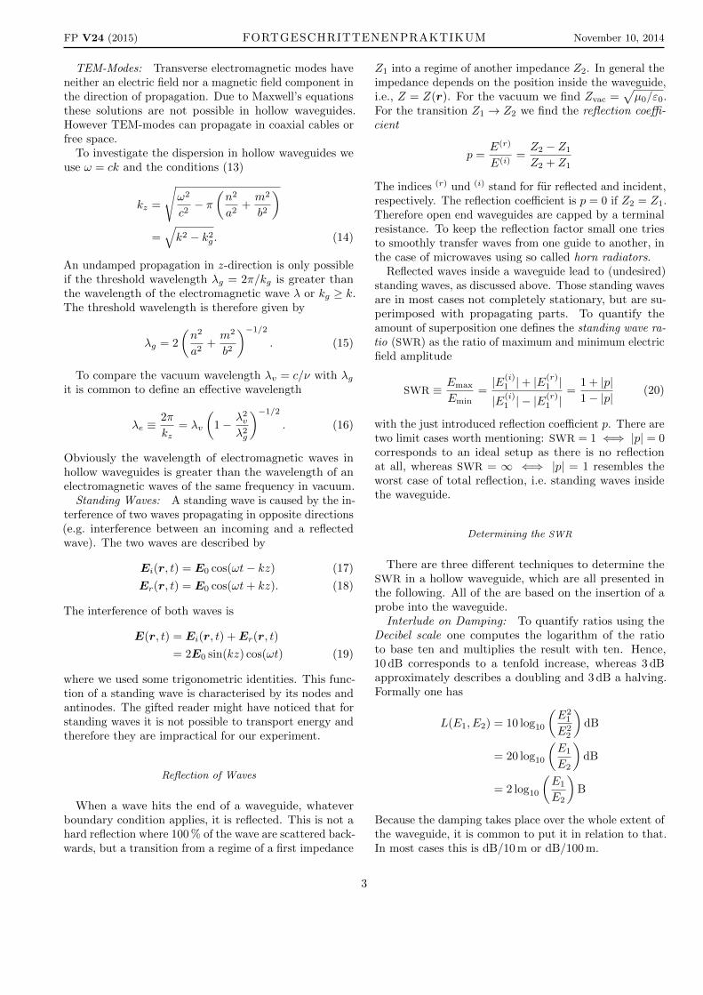
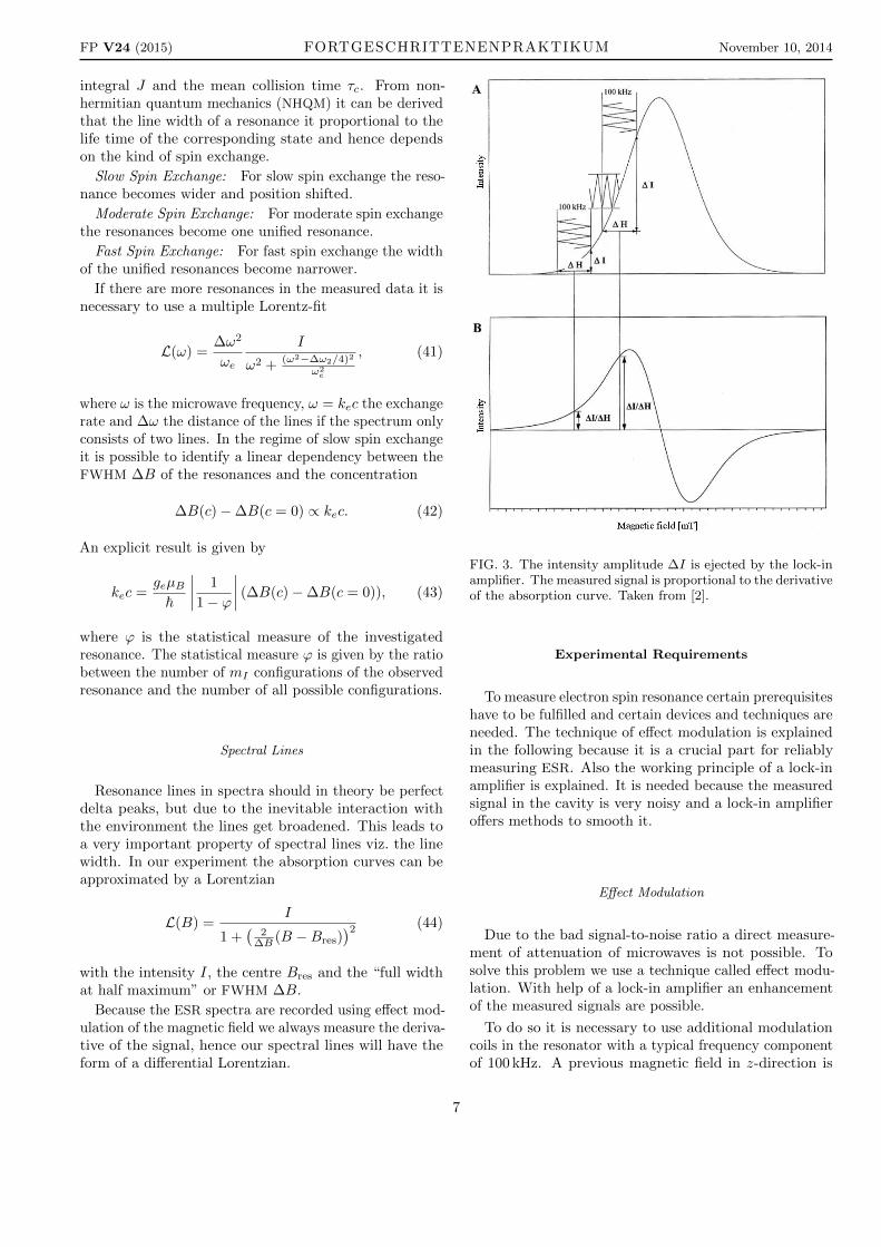
FIG. 3. The intensity amplitude ∆I is ejected by the lock-inamplifier. The measured signal is proportional to the derivativeof the absorption curve. Taken from [2].

Experimental Requirements

To measure electron spin resonance certain prerequisiteshave to be fulfilled and certain devices and techniques areneeded. The technique of effect modulation is explainedin the following because it is a crucial part for reliablymeasuring ESR. Also the working principle of a lock-inamplifier is explained. It is needed because the measuredsignal in the cavity is very noisy and a lock-in amplifieroffers methods to smooth it.

Effect Modulation

Due to the bad signal-to-noise ratio a direct measure-ment of attenuation of microwaves is not possible. Tosolve this problem we use a technique called effect modu-lation. With help of a lock-in amplifier an enhancementof the measured signals are possible.

To do so it is necessary to use additional modulationcoils in the resonator with a typical frequency componentof 100 kHz. A previous magnetic field in z-direction is

7


then modified such that it is given by

B(t) = Bstat + ∆B

(t

t0− 1

2

)+

1

2Bm sin(ωmt), (45)

where ωm is the modulation frequency which is muchfaster than the linear change of the magnetic field, Bmthe modulation amplitude which is small compared to thewidth of the resonance and ∆B is the measured timeframe,c.f. figure 3. The figure shows that the modulation of themagnetic field also causes a modulation of the absorbedmicrowave power. Disorders caused by other sources thanthe ESR absorption of the microwave are not modulated.It is also depicted that the issued voltage of the lock-inamplifier is proportional to the derivative of the absorptioncurve. The absorption curve is a result of numerical orelectronic integration.

Lock-In Amplifier

A lock-in amplifier is a technical device used to detectand measure small AC signals down to a few nanovolts.With their help it is possible to extract signals with knowncarrier waves from noisy environments. Therefore theyuse a technique known as phase-sensitive detection.

An common lock-in amplifier amplifies and then multi-plies the incoming signal

Usig = Usig,0 sin(ωsigt+ θsig) (46)

from an experiment (e.g. an oscillator) with a lock-inreference

Uref = Uref,0 sin(ωreft+ θref), (47)

where Usig,0 is the signal amplitude. Note that the refer-ence signal in the experiment is the signal of the magneticfield modulation and the incoming signal is the measuredmicrowave power excited from the magnetic field modula-tion. Multiplying both signals yield

UM = Usig,0Uref,0 sin(ωsigt+ θsig) sin(ωreft+ θref).

With the help of some trigonometrical identities we canrewrite the signal

UM =1

2

[U cos((ωsig − ωref)t+ θsig − θref)

− U cos((ωsig + ωref)t+ θsig + θref)], (48)

where U = Usig,0Usig,0. The signal UM is passed througha low pass filter which only let a signal pass if ωsig = ωref ,i.e. , the filtered output will be a very nice DC signal

UOut =1

2U cos(θsig − θref). (49)

To maximise the output signal UOut the condition (θsig −θref = 2πn and n ∈ N has to be fulfilled. This can beachieved with a manual phase shifting device or usinga second lock-in amplifier with an π/2 phase shifted fixreference signal. Unfortunately in the experimental set-uponly a manual phase shifting device is possible.

ANALYSIS

Experiments on ESR I

In this section we deal with experiments which areneeded in preparation for actual ESR spectra. Importantquantities to determine are the Q-factors of our samples.This can be done without any magnetic field. As all subse-quent measurements depend on a magnetic field, which isadjusted via its Hall voltage, we need to calibrate the Hallprobe using the well gauged DPPH. Next a set of optimalsystem parameters is to be found, such that the qualityof ESR spectra is maximised with respect to power ofthe microwave radiation, as well as modulation frequency,Hall voltage, and amplitude of the magnetic field, andultimately delay time of the lock-in amplifier. Afterwardsthe first ESR spectra are recorded to analyse the hyperfinestructure in DPPH depending on the concentration, andcompute the g-Tensor of CuSO4 and Mn2+.

Experimental Setup

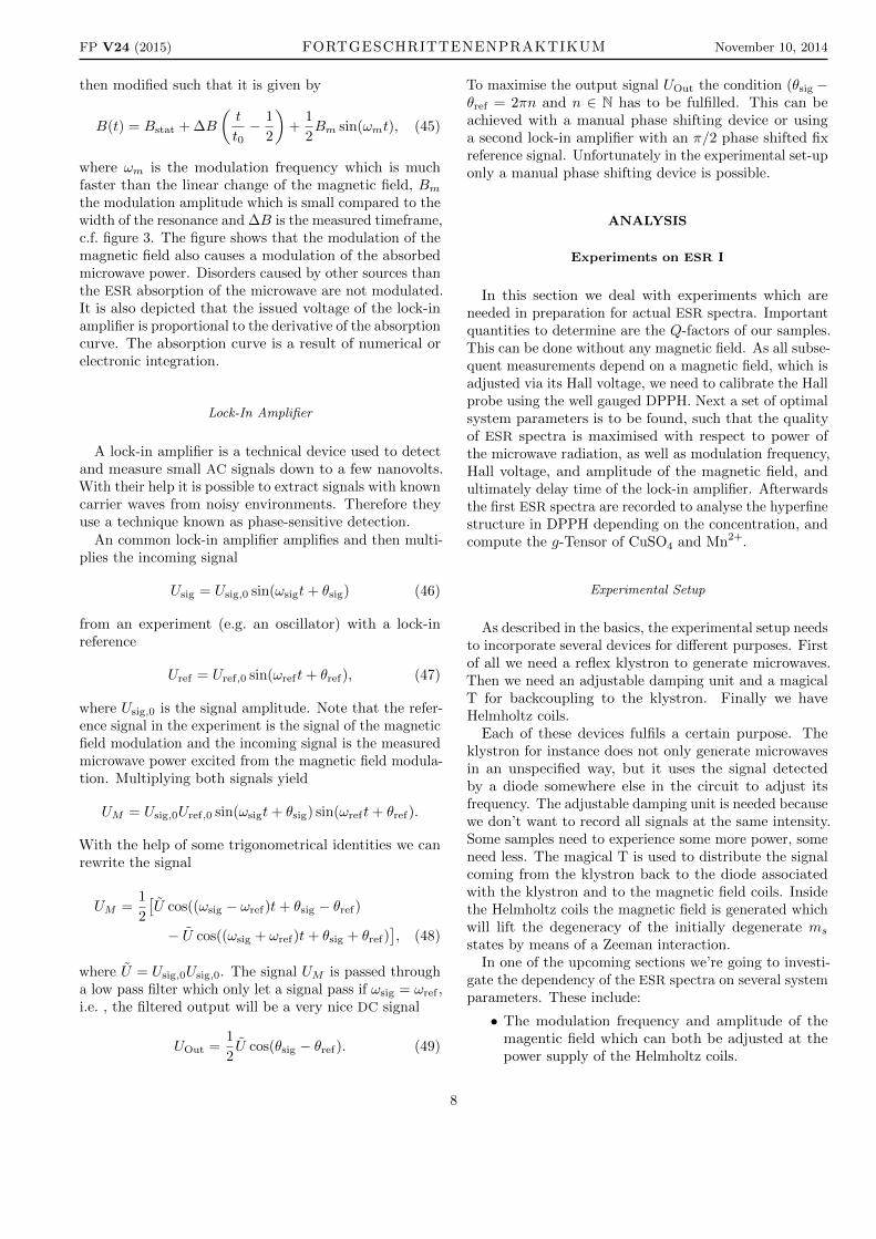
As described in the basics, the experimental setup needsto incorporate several devices for different purposes. Firstof all we need a reflex klystron to generate microwaves.Then we need an adjustable damping unit and a magicalT for backcoupling to the klystron. Finally we haveHelmholtz coils.

Each of these devices fulfils a certain purpose. Theklystron for instance does not only generate microwavesin an unspecified way, but it uses the signal detectedby a diode somewhere else in the circuit to adjust itsfrequency. The adjustable damping unit is needed becausewe don’t want to record all signals at the same intensity.Some samples need to experience some more power, someneed less. The magical T is used to distribute the signalcoming from the klystron back to the diode associatedwith the klystron and to the magnetic field coils. Insidethe Helmholtz coils the magnetic field is generated whichwill lift the degeneracy of the initially degenerate ms

states by means of a Zeeman interaction.In one of the upcoming sections we’re going to investi-

gate the dependency of the ESR spectra on several systemparameters. These include:

• The modulation frequency and amplitude of themagentic field which can both be adjusted at thepower supply of the Helmholtz coils.

8


FIG. 4. Photo of the experimental setup. Not all componentsare visible in the picture. The black can on the far left are theHelmholtz coils for the magnetic field. A little right to it wesee the magical T. In the middle is the adjustable dampingmodule and on the far left the klystron. The whole setup wasmuch larger and included all sorts of measurement devices andpower sources—these are not illustrated.

• The microwave power can be adjusted using theaforementioned damping unit.

• The integration time of the signal can be selectedon the lock-in amplifier.

Another free parameter was the magentic field sweepwhich was selected on the computer interface, but thishad no effect on the actual outcome of the measurement.

Quality of the resonator

The quality factor Q of a resonator characterises thebandwidth relative to its resonance frequency and thus isa dimensionless quantity. We use the definition

Q ≡ ν0

∆ν, (50)

where ν0 is the resonance frequency and ∆ν the bandwidth(FWHM). The higher the Q-factor, the lower are thedissipative losses in the resonator. The investigation ofthe different samples with ESR extract energy from themodes in the resonator and will lead to a decreasingquality factor.

In the following subsection we want to determine theQ-factor for an empty resonator and filled resonator withthe samples DPPH (poly), CuSO4 (poly) and Mn2+ (aq).To do so, it is necessary to adjust the klystron frequencyby modifying the resonator geometry. The goal of thisadjustment is to shift the absorption dip of the resonatorto the most powerful klystron mode. For this purpose weuse an oscilloscope. With help of an additional measure-ment resonator it is possible to detect the resonator mode.With help of a micrometre we can adjust the position of

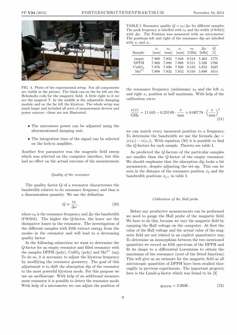
TABLE I. Resonator quality Q = ν0/∆ν for different samples.The peak frequency is labelled with ν0 and the width (FWHM)with ∆ν. The Position was measured with an micrometer.The positions left and right of the resonance dip are labelledwith xl and xr.

xl x0 xr ν0 ∆ν QSample [mm] [mm] [mm] [GHz] [kHz] [1]

empty 7.808 7.832 7.848 9.518 5.363 1775DPPH 7.868 7.888 7.908 9.511 5.326 1786CuSO4 7.876 7.896 7.920 9.510 5.852 1625Mn2+ 7.808 7.832 7.852 9.518 5.898 1614

the resonance frequency (minimum) x0 and the left xland right xr position at half maximum. With help of thecalibration curve

ν(x)

GHz= 11.045− 0.255 89 · x

mm+ 0.007 78 ·

( x

mm

)2

(51)

we can match every measured position to a frequency.To determine the bandwidth we use the formula ∆ν =|ν(xl)− ν(xr)|. With equation (50) it is possible to findthe Q-factors for each sample. Thereto see table I.

As predicted the Q-factors of the particular samplesare smaller than the Q-factor of the empty resonator.We should emphasise that the absorption dip looks a bitasymmetric, despite adjusting the set-up. This can beseen in the distance of the resonance position x0 and thebandwidth positions xl/r in table I.

Calibration of the Hall probe

Before any productive measurements can be performedwe need to gauge the Hall probe of the magnetic field.We have to do this, because we vary the magnetic field byramping the Hall voltage on the computer. At first thevalue of the Hall voltage and the actual value of the mag-netic field are not related in an explicit quantitative way.To determine an isomorphism between the two mentionedquantities we record an ESR spectrum of the DPPH andfit its shape to a differential Lorentzian to obtain themaximum of the resonance (root of the fitted function).This will give us an estimate for the magnetic field as allmicroscopic quantities of DPPH have been studied thor-oughly in previous experiments. The important propertyhere is the Lande-g-factor which was found to be [3]

gDPPH = 2.0036 . (52)

9


−8

−6

−4

−2

0

2

4

6

8

334 336 338 340 342

133 133.5 134 134.5 135 135.5 136 136.5 137D

iffer

enti

al

abso

rpti

on

dI/

dB

[a.u.]

Magentic field B [mT]

Hall voltage UH [mV]

B(UH) = 339 mT

UH = 135.13 mV

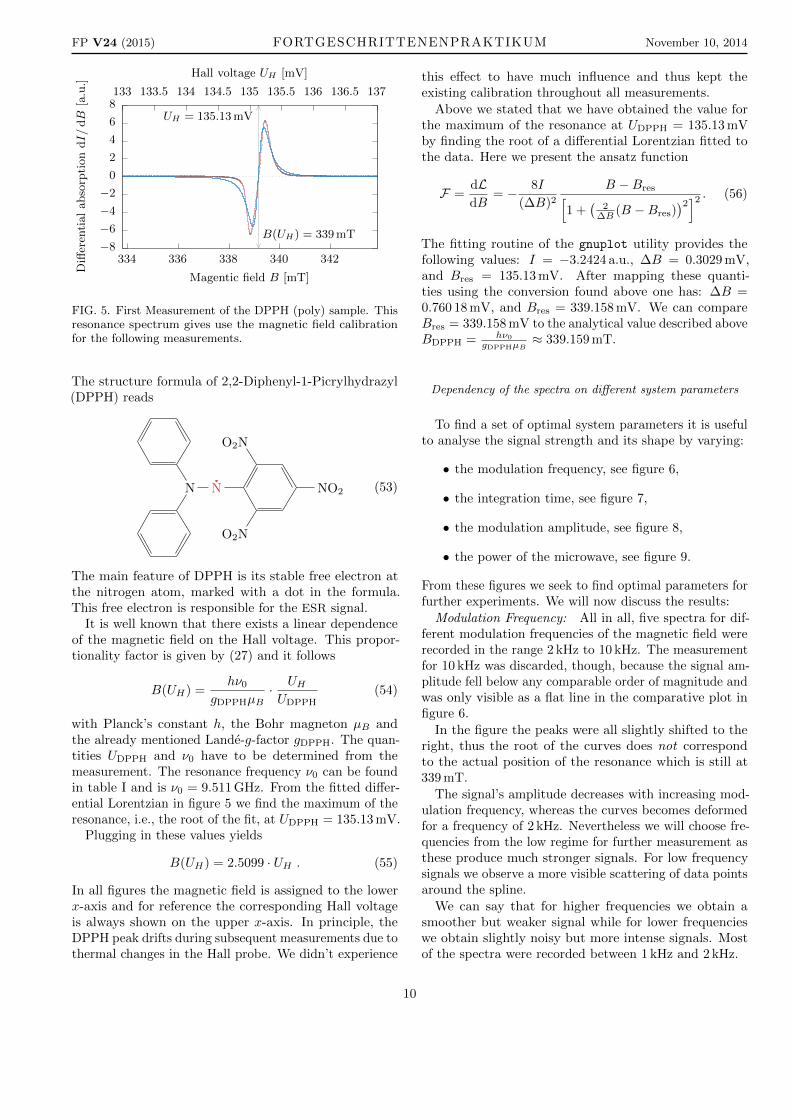
FIG. 5. First Measurement of the DPPH (poly) sample. Thisresonance spectrum gives use the magnetic field calibrationfor the following measurements.

The structure formula of 2,2-Diphenyl-1-Picrylhydrazyl(DPPH) reads

N N

NO2

NO2

NO2

(53)

The main feature of DPPH is its stable free electron atthe nitrogen atom, marked with a dot in the formula.This free electron is responsible for the ESR signal.

It is well known that there exists a linear dependenceof the magnetic field on the Hall voltage. This propor-tionality factor is given by (27) and it follows

B(UH) =hν0

gDPPHµB· UHUDPPH

(54)

with Planck’s constant h, the Bohr magneton µB andthe already mentioned Lande-g-factor gDPPH. The quan-tities UDPPH and ν0 have to be determined from themeasurement. The resonance frequency ν0 can be foundin table I and is ν0 = 9.511 GHz. From the fitted differ-ential Lorentzian in figure 5 we find the maximum of theresonance, i.e., the root of the fit, at UDPPH = 135.13 mV.

Plugging in these values yields

B(UH) = 2.5099 · UH . (55)

In all figures the magnetic field is assigned to the lowerx-axis and for reference the corresponding Hall voltageis always shown on the upper x-axis. In principle, theDPPH peak drifts during subsequent measurements due tothermal changes in the Hall probe. We didn’t experience

this effect to have much influence and thus kept theexisting calibration throughout all measurements.

Above we stated that we have obtained the value forthe maximum of the resonance at UDPPH = 135.13 mVby finding the root of a differential Lorentzian fitted tothe data. Here we present the ansatz function

F =dLdB

= − 8I

(∆B)2

B −Bres[1 +

(2

∆B (B −Bres))2]2 . (56)

The fitting routine of the gnuplot utility provides thefollowing values: I = −3.2424 a.u., ∆B = 0.3029 mV,and Bres = 135.13 mV. After mapping these quanti-ties using the conversion found above one has: ∆B =0.760 18 mV, and Bres = 339.158 mV. We can compareBres = 339.158 mV to the analytical value described aboveBDPPH = hν0

gDPPHµB≈ 339.159 mT.

Dependency of the spectra on different system parameters

To find a set of optimal system parameters it is usefulto analyse the signal strength and its shape by varying:

• the modulation frequency, see figure 6,

• the integration time, see figure 7,

• the modulation amplitude, see figure 8,

• the power of the microwave, see figure 9.

From these figures we seek to find optimal parameters forfurther experiments. We will now discuss the results:

Modulation Frequency: All in all, five spectra for dif-ferent modulation frequencies of the magnetic field wererecorded in the range 2 kHz to 10 kHz. The measurementfor 10 kHz was discarded, though, because the signal am-plitude fell below any comparable order of magnitude andwas only visible as a flat line in the comparative plot infigure 6.

In the figure the peaks were all slightly shifted to theright, thus the root of the curves does not correspondto the actual position of the resonance which is still at339 mT.

The signal’s amplitude decreases with increasing mod-ulation frequency, whereas the curves becomes deformedfor a frequency of 2 kHz. Nevertheless we will choose fre-quencies from the low regime for further measurement asthese produce much stronger signals. For low frequencysignals we observe a more visible scattering of data pointsaround the spline.

We can say that for higher frequencies we obtain asmoother but weaker signal while for lower frequencieswe obtain slightly noisy but more intense signals. Mostof the spectra were recorded between 1 kHz and 2 kHz.

10


−10

−8

−6

−4

−2

0

2

4

6

8

10

337 338 339 340 341 342 343

134 134.5 135 135.5 136 136.5 137D

iffer

enti

al

abso

rpti

on

dI/

dB

[a.u.]



2000 a.u.4000 a.u.5000 a.u.6000 a.u.8000 a.u.

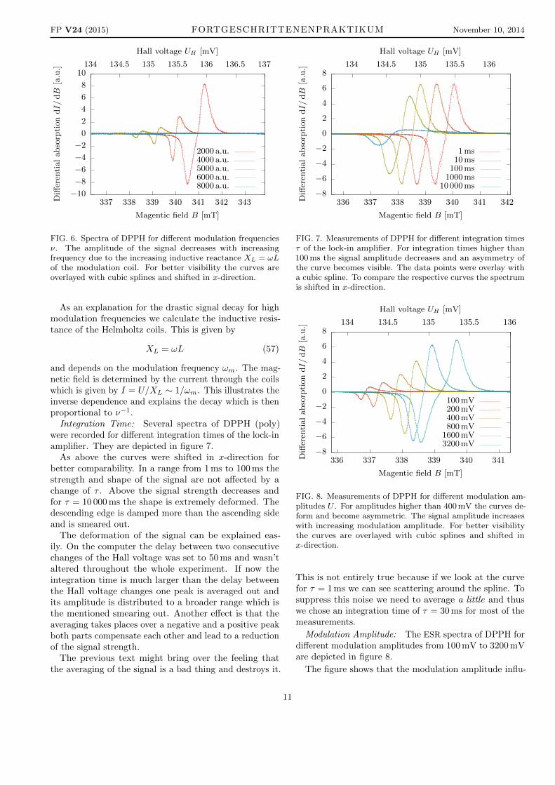
FIG. 6. Spectra of DPPH for different modulation frequenciesν. The amplitude of the signal decreases with increasingfrequency due to the increasing inductive reactance XL = ωLof the modulation coil. For better visibility the curves areoverlayed with cubic splines and shifted in x-direction.

As an explanation for the drastic signal decay for highmodulation frequencies we calculate the inductive resis-tance of the Helmholtz coils. This is given by

XL = ωL (57)

and depends on the modulation frequency ωm. The mag-netic field is determined by the current through the coilswhich is given by I = U/XL ∼ 1/ωm. This illustrates theinverse dependence and explains the decay which is thenproportional to ν−1.

Integration Time: Several spectra of DPPH (poly)were recorded for different integration times of the lock-inamplifier. They are depicted in figure 7.

As above the curves were shifted in x-direction forbetter comparability. In a range from 1 ms to 100 ms thestrength and shape of the signal are not affected by achange of τ . Above the signal strength decreases andfor τ = 10 000 ms the shape is extremely deformed. Thedescending edge is damped more than the ascending sideand is smeared out.

The deformation of the signal can be explained eas-ily. On the computer the delay between two consecutivechanges of the Hall voltage was set to 50 ms and wasn’taltered throughout the whole experiment. If now theintegration time is much larger than the delay betweenthe Hall voltage changes one peak is averaged out andits amplitude is distributed to a broader range which isthe mentioned smearing out. Another effect is that theaveraging takes places over a negative and a positive peakboth parts compensate each other and lead to a reductionof the signal strength.

The previous text might bring over the feeling thatthe averaging of the signal is a bad thing and destroys it.

−8

−6

−4

−2

0

2

4

6

8

336 337 338 339 340 341 342

134 134.5 135 135.5 136

Diff

eren

tial

abso

rpti

on

dI/

dB

[a.u.]



1 ms10 ms

100 ms1000 ms

10 000 ms

FIG. 7. Measurements of DPPH for different integration timesτ of the lock-in amplifier. For integration times higher than100 ms the signal amplitude decreases and an asymmetry ofthe curve becomes visible. The data points were overlay witha cubic spline. To compare the respective curves the spectrumis shifted in x-direction.

−8

−6

−4

−2

0

2

4

6

8

336 337 338 339 340 341

134 134.5 135 135.5 136

Diff

eren

tial

abso

rpti

on

dI/

dB

[a.u.]



100 mV200 mV400 mV800 mV

1600 mV3200 mV

FIG. 8. Measurements of DPPH for different modulation am-plitudes U . For amplitudes higher than 400 mV the curves de-form and become asymmetric. The signal amplitude increaseswith increasing modulation amplitude. For better visibilitythe curves are overlayed with cubic splines and shifted inx-direction.

This is not entirely true because if we look at the curvefor τ = 1 ms we can see scattering around the spline. Tosuppress this noise we need to average a little and thuswe chose an integration time of τ = 30 ms for most of themeasurements.

Modulation Amplitude: The ESR spectra of DPPH fordifferent modulation amplitudes from 100 mV to 3200 mVare depicted in figure 8.

The figure shows that the modulation amplitude influ-

11


−10

−8

−6

−4

−2

0

2

4

6

8

336 337 338 339 340

134 134.5 135 135.5D

iffer

enti

al

abso

rpti

on

dI/

dB

[a.u.]



10 dB12 dB14 dB16 dB18 dB

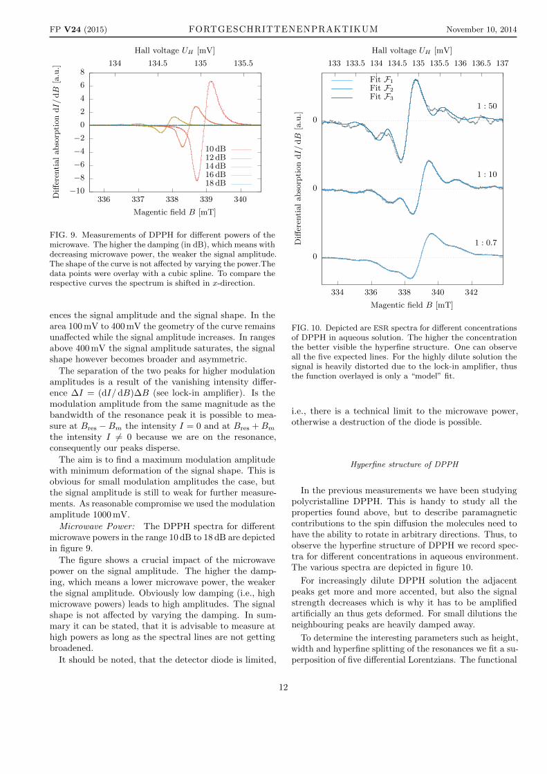
FIG. 9. Measurements of DPPH for different powers of themicrowave. The higher the damping (in dB), which means withdecreasing microwave power, the weaker the signal amplitude.The shape of the curve is not affected by varying the power.Thedata points were overlay with a cubic spline. To compare therespective curves the spectrum is shifted in x-direction.

ences the signal amplitude and the signal shape. In thearea 100 mV to 400 mV the geometry of the curve remainsunaffected while the signal amplitude increases. In rangesabove 400 mV the signal amplitude saturates, the signalshape however becomes broader and asymmetric.

The separation of the two peaks for higher modulationamplitudes is a result of the vanishing intensity differ-ence ∆I = (dI/dB)∆B (see lock-in amplifier). Is themodulation amplitude from the same magnitude as thebandwidth of the resonance peak it is possible to mea-sure at Bres −Bm the intensity I = 0 and at Bres +Bmthe intensity I 6= 0 because we are on the resonance,consequently our peaks disperse.

The aim is to find a maximum modulation amplitudewith minimum deformation of the signal shape. This isobvious for small modulation amplitudes the case, butthe signal amplitude is still to weak for further measure-ments. As reasonable compromise we used the modulationamplitude 1000 mV.

Microwave Power: The DPPH spectra for differentmicrowave powers in the range 10 dB to 18 dB are depictedin figure 9.

The figure shows a crucial impact of the microwavepower on the signal amplitude. The higher the damp-ing, which means a lower microwave power, the weakerthe signal amplitude. Obviously low damping (i.e., highmicrowave powers) leads to high amplitudes. The signalshape is not affected by varying the damping. In sum-mary it can be stated, that it is advisable to measure athigh powers as long as the spectral lines are not gettingbroadened.

It should be noted, that the detector diode is limited,

0

0

0

334 336 338 340 342

133 133.5 134 134.5 135 135.5 136 136.5 137

Diff

eren

tial

abso

rpti

on

dI/

dB

[a.u.]



1 : 0.7

1 : 10

1 : 50

Fit F1

Fit F2

Fit F3

FIG. 10. Depicted are ESR spectra for different concentrationsof DPPH in aqueous solution. The higher the concentrationthe better visible the hyperfine structure. One can observeall the five expected lines. For the highly dilute solution thesignal is heavily distorted due to the lock-in amplifier, thusthe function overlayed is only a “model” fit.

i.e., there is a technical limit to the microwave power,otherwise a destruction of the diode is possible.

Hyperfine structure of DPPH

In the previous measurements we have been studyingpolycristalline DPPH. This is handy to study all theproperties found above, but to describe paramagneticcontributions to the spin diffusion the molecules need tohave the ability to rotate in arbitrary directions. Thus, toobserve the hyperfine structure of DPPH we record spec-tra for different concentrations in aqueous environment.The various spectra are depicted in figure 10.

For increasingly dilute DPPH solution the adjacentpeaks get more and more accented, but also the signalstrength decreases which is why it has to be amplifiedartificially an thus gets deformed. For small dilutions theneighbouring peaks are heavily damped away.

To determine the interesting parameters such as height,width and hyperfine splitting of the resonances we fit a su-perposition of five differential Lorentzians. The functional

12


form is given by

F =dLdB

= −5∑i=1

8Ii(∆Bi)2

B −Bres,i[1 +

(2

∆Bi(B −Bres,i)

)2]2 .

(58)where the parameter for the width is composed of severalcomponents

Bres,i =

Bres + 2A1 for i = 1

Bres +A2 for i = 2

Bres for i = 3

Bres +A4 for i = 4

Bres + 2A5 for i = 5

(59)

This form helps us with the determination of the hyperfinesplitting because these are now parameters of the fit. Thefitted curves are overlayed with the data in figure 10. Forthe concentration 1 : 50 a “model” fit was imposed asone can see the data is not suited for good convergence,i.e. the fit parameters for this case are educated guessesbased on the assumption that the width of the peaks andthe hyperfine splitting should increase with decreasingconcentration. The values were then augmented from theother two measurements. The height of the peaks wasdrawn by eye.

The values for the fit parameters are listed in table II.The width of the resonances and the hyperfine splittingwere averaged over all five and four values, respectively.The approximate ratio of the intensity of the peaks canalso be found there.

For the ratio of the intensities we expect 1 : 2 : 3 : 2 : 1.This is, unfortunately, in no way met. Because even theerror has a huge scattering this has to be a systematicerror and cannot be explained using a statistical argument.Even though the ratio is so far off we can still drawconclusions from it. For example we can definitely factorout that two resonances have the same height, thus theelectron couples to at least two cores. Also, the fact thatthere are five resonances gives us 2(I1 + I2) + 1 = 5,yielding I1 = I2 = 1. Thus the electron couples to thenitrogen atoms because these have a nuclear spin of I = 1.

For the value of hyperfine splitting we choose the resultsof the fit to the 1 : 10 sample as this possesses the bestratio of convergence of the fit and spectral line width.We average over the four values, because the hyperfinesplitting should be equidistant for all reosnances.

ADPPH = 1.720 mT

the hyperfine splitting of DPPH reaches from 1.12 mT to1.73 mT as reported in [4]. This means that our valuesare within the range of possible results.

−8

−6

−4

−2

0

2

4

6

8

280 290 300 310 320 330 340 350

110 115 120 125 130 135 140

Diff

eren

tial

abso

rpti

on

dI/

dB

[a.u.]



g⊥ = 2.27

g‖ = 2.09

CuSO4

Fit F1

Fit F2

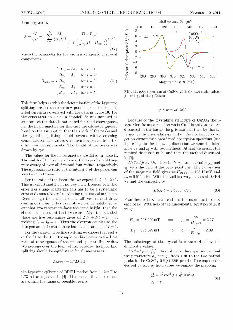
FIG. 11. ESR-spectrum of CuSO4 with the two main valuesg⊥ and g‖ of the g-Tensor.

g-Tensor of Cu2+

Because of the crystalline structure of CuSO4 the g-factor for the unpaired electron in Cu2+ is anisotropic. Asdiscussed in the basics the g-tensor can then be charac-terised by the eigenvalues g⊥ and g‖. As a consequence weget an asymmetric broadened absorption spectrum (seefigure 11). In the following discussion we want to deter-mine g⊥ and p‖ with two methods. At first we present themethod discussed in [5] and then the method discussedin [6].

Method from [5]: Like in [5] we can determine g⊥ andg‖ with the help of the peak positions. The calibrationof the magnetic field gives us UDPPH = 135.13 mV andν0 = 9.511 GHz. With the well known g-factors of DPPHwe find the connectivity

B(UH) = 2.5099 · UH . (60)

From figure 11 we can read out the magnetic fields toeach peak. With help of the fundamental equation of ESR

we get

B⊥ = 298.929 mT =⇒ g⊥ =hν

B⊥µB= 2.27,

B‖ = 325.049 mT =⇒ g‖ =hν

B‖µB= 2.09.

The anisotropy of the crystal is characterised by thedifferent g-values.

Method from [6]: According to the paper we can findthe parameters gα and gγ from a fit to the two partialpeaks in the CuSO4 ·5 H2O ESR profile. To compute thedesired g⊥ and g‖ from those we employ the mapping

g2α = g2

‖ cos2 ϕ+ g2⊥ sin2 ϕ

gγ = g⊥(61)

13


TABLE II. Listed below are the parameters of the fit (58) for the various concentrations of DPPH. In the last row of each tablethe estimated peak intensity ratio, the mean values of the FWHM, and the hyperfine splitting are presented. The centre of eachresonance is given in the top row.

1 : 0.7 – Bres = 338.96 mT

Ii ∆Bi Ai

[a.u.] [mT] [mT]

1 −0.127 1.291 1.7382 −0.749 1.757 1.4743 −6.519 2.381 –4 −0.472 1.676 1.7125 −0.073 1.201 1.867

1:6:51:4:1 1.661 1.698

1 : 10 – Bres = 338.95 mT

Ii ∆Bi Ai

[a.u.] [mT] [mT]

1 −0.366 1.461 1.7282 −1.274 1.526 1.4563 −5.816 1.794 –4 −0.884 1.583 1.7635 −0.288 1.896 1.933

1:3:16:3:1 1.652 1.720

1 : 50 – Bres = 338.20 mT

Ii ∆Bi Ai

[a.u.] [mT] [mT]

1 −0.347 1.512 1.7392 −1.709 1.319 1.4483 −7.704 1.590 –4 −1.397 1.474 1.7185 −0.447 1.869 1.875

1:5:22:4:1 1.553 1.695

where ϕ = 41° as extracted from table 1 in [6]. Accordingto (27) we need the magnetic field at the level transition,which is the zeros of the differential profile (i.e., peaksof the intensity profile). These can be obtained from afit to the two respective peaks and were extracted at thepoints Bαres = 302.851 mT and Bγres = 322.947 mT. Withf0 = 9.510 GHz we obtain

gα =hν0

BαresµB= 2.24 (62)

gγ =hµ0

BγresµB= 2.10 (63)

Now we apply the mapping introduced above (61) tocalculate the g-Tensor:

g⊥ = gγ = 2.10 (64)

gα =

√g2α − g2

⊥ sin2 ϕ

cos2 ϕ= 2.24 (65)

Comparing this to the literature values in table 1 in [6]g⊥ = 2.05 and g‖ = 2.38 yields the relative deviationsQ(g⊥, g⊥) = 2.4 % and Q(g‖, g‖) = 5.9 %. This is unfor-tunately not within the error range given in the paper.This might be due to the fact that we didn’t recalibratethe magnetic again and the thermal drift kicked in.

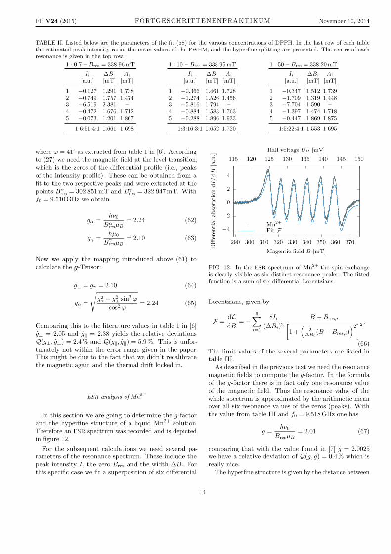
ESR analysis of Mn2+

In this section we are going to determine the g-factorand the hyperfine structure of a liquid Mn2+ solution.Therefore an ESR spectrum was recorded and is depictedin figure 12.

For the subsequent calculations we need several pa-rameters of the resonance spectrum. These include thepeak intensity I, the zero Bres and the width ∆B. Forthis specific case we fit a superposition of six differential

−4

−2

0

2

4

290 300 310 320 330 340 350 360 370

115 120 125 130 135 140 145 150

Diff

eren

tial

abso

rpti

on

dI/

dB

[a.u.]



Mn2+

Fit F

FIG. 12. In the ESR spectrum of Mn2+ the spin exchangeis clearly visible as six distinct resonance peaks. The fittedfunction is a sum of six differential Lorentzians.

Lorentzians, given by

F =dLdB

= −6∑i=1

8Ii(∆Bi)2

B −Bres,i[1 +

(2

∆Bi(B −Bres,i)

)2]2 .

(66)The limit values of the several parameters are listed intable III.

As described in the previous text we need the resonancemagnetic fields to compute the g-factor. In the formulaof the g-factor there is in fact only one resonance valueof the magnetic field. Thus the resonance value of thewhole spectrum is approximated by the arithmetic meanover all six resonance values of the zeros (peaks). Withthe value from table III and f0 = 9.518 GHz one has

g =hν0

BresµB= 2.01 (67)

comparing that with the value found in [7] g = 2.0025we have a relative deviation of Q(g, g) = 0.4 % which isreally nice.

The hyperfine structure is given by the distance between

14


TABLE III. Listed below are the parameters of the fit (66).The ratio of the respective intensities, the arithmetic mean ofthe width, the resonance values, and the hyperfine splittingare listed in the last row of the table. These are needed forfurther calculations.

Ii ∆Bi Bres,i Ai

[a.u.] [mT] [mT] [mT]

1 20.48 7.24 314.94 8.602 21.21 7.73 323.54 9.073 20.70 7.55 332.61 9.274 21.16 7.52 341.88 9.525 21.83 7.46 351.40 9.946 24.67 8.53 361.34 –

1:1:1:1:1:1 7.67 337.62 9.28

adjacent absorption peaks, i.e., zeros of the differentialabsorption. In theory all of those should be the same.This is obviously not met as can easily be seen fromtable III. Thus we present the arithmetic mean of allthose values as our hyperfine structure splitting.

A = 9.28 mT (68)

Here A3 can be compared to the literature value found in[8, p. 43] A3 = 8.69 mT which yields a relative deviationof Q(A3, A3) = 6.7 %.

Spin Density at the Core

The hyperfine splitting is readily connected with theFermi contact interaction. It describes the spin-spin cou-pling of the electron and the core at the position of thecore. Hence we can calculate the probability of presenceof the electron at the core using the measured values ofthe hyperfine splitting of DPPH and Mn2+. The termspin density is not chosen very wisely in this context asit does not describe a spacial density of “matter”, but aprobability density of presence of one particle at the core.This is denoted by |ψ(0)|2. The formula for this quantityis taken from [9].

|ψ(0)|2 =3

2

A

µ0gIµK(69)

with the Lande-factor gI of the core, the core magnetonµK and the magnetic field constant µ0.

With the values from the previous text we can deter-mine the spin density for DPPH and Mn2+. As a reminder,the values are

ADPPH = 1.72 mT (70)

AMn2+ = 9.28 mT (71)

Plugging these into the formula for the spin density,together with the constants gI,DPPH = 0.4038 and

gI,Mn2+ = 1.3819 one has:

|ψDPPH(0)|2 = 1.007 · 1030 m−3, (72)

|ψMn2+(0)|2 = 1.587 · 1030 m−3. (73)

In the case of Mn2+ the paramagnetic electrons are inthe d orbital and hence the presence of the electrons atthe core is zero. Consequently the Fermi contact inter-action is in this case not possible (only for s electrons).For electrons in the p, d, f ,. . . -orbitals the dipole-dipoleinteraction of the electrons and the nuclear moments is re-sponsible for the hyperfine splitting and the not vanishingvalue of |ψMn2+(0)|2 [9].

Experiments on ESR II

In the present section we seek to study the spin ex-change in TEMPO and its impact on the form of thespectral lines in an ESR spectrum. We are going to quan-tify the spin diffusion by analysing the line widths of thehyperfine splitting.

The substance in use it TEMPO, which is an acronymfor (2,2,6,6-Tetramethylpiperidin-1-yl)oxyl. The structureformula reads

CH3

CH3N

O

CH3

CH3

(74)

The unpaired electron of the oxygen is responsible forthe ESR signal. ESR spectra are recorded for differentconcentrations of TEMPO in toluene solution rangingfrom 0.25 mmol l−1 to 250 mmol l−1. As O has a nuclearspin of I = 0 the only coupling for the electron is possiblyto the adjacent N core with nuclear spin I = 1. Thus2 · 1 + 1 = 3 hyperfine peaks can be observed.

Dependency of the spectra on the TEMPO concentration

Visibility and line width of the hyperfine splitting iscritically dependent on the spin exchange rate, whichin turn is dependent on the concentration of the ESR

active substance. A plot of all measurements for varyingconcentration are shown in figure 13 in a waterfall plot. Itis visible that for decreasing concentration the amplitudedrops but also for c ≤ 25 mmol l−1 we find three resonancepeaks of approximately same height.

From these observations we feel confident to draw thefollowing conclusions:

• Slow Spin Exchange: For concentrations in therange of 0.25 mmol l−1 to 25 mmol l−1 we can see

15


0

0

0

0

0

0

0

0

0

332 333 334 335 336 337

132 132.5 133 133.5 134 134.5D

iffer

enti

al

abso

rpti

on

dI/

dB

[a.u.]



250 mmoll

175 mmoll

125 mmoll

83 mmoll

50 mmoll

25 mmoll

10 mmoll

5 mmoll

0.25 mmoll

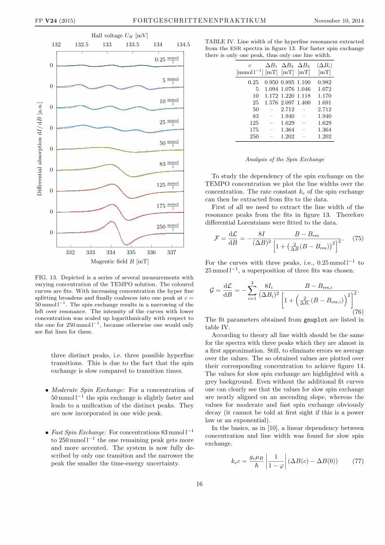
FIG. 13. Depicted is a series of several measurements withvarying concentration of the TEMPO solution. The colouredcurves are fits. With increasing concentration the hyper finesplitting broadens and finally coalesces into one peak at c =50 mmol l−1. The spin exchange results in a narrowing of theleft over resonance. The intensity of the curves with lowerconcentration was scaled up logarithmically with respect tothe one for 250 mmol l−1, because otherwise one would onlysee flat lines for these.

three distinct peaks, i.e. three possible hyperfinetransitions. This is due to the fact that the spinexchange is slow compared to transition times.

• Moderate Spin Exchange: For a concentration of50 mmol l−1 the spin exchange is slightly faster andleads to a unification of the distinct peaks. Theyare now incorporated in one wide peak.

• Fast Spin Exchange: For concentrations 83 mmol l−1

to 250 mmol l−1 the one remaining peak gets moreand more accented. The system is now fully de-scribed by only one transition and the narrower thepeak the smaller the time-energy uncertainty.

TABLE IV. Line width of the hyperfine resonances extractedfrom the ESR spectra in figure 13. For faster spin exchangethere is only one peak, thus only one line width.

c ∆B1 ∆B2 ∆B3 〈∆Bi〉[mmol l−1] [mT] [mT] [mT] [mT]

0.25 0.950 0.895 1.100 0.9825 1.094 1.076 1.046 1.072

10 1.172 1.220 1.118 1.17025 1.576 2.097 1.400 1.69150 – 2.712 – 2.71283 – 1.940 – 1.940

125 – 1.629 – 1.629175 – 1.364 – 1.364250 – 1.202 – 1.202

Analysis of the Spin Exchange

To study the dependency of the spin exchange on theTEMPO concentration we plot the line widths over theconcentration. The rate constant ke of the spin exchangecan then be extracted from fits to the data.

First of all we need to extract the line width of theresonance peaks from the fits in figure 13. Thereforedifferential Lorentzians were fitted to the data.

F =dLdB

= − 8I

(∆B)2

B −Bres[1 +

(2

∆B (B −Bres))2]2 . (75)

For the curves with three peaks, i.e., 0.25 mmol l−1 to25 mmol l−1, a superposition of three fits was chosen.

G =dLdB

= −3∑i=1

8Ii(∆Bi)2

B −Bres,i[1 +

(2

∆Bi(B −Bres,i)

)2]2 .

(76)The fit parameters obtained from gnuplot are listed intable IV.

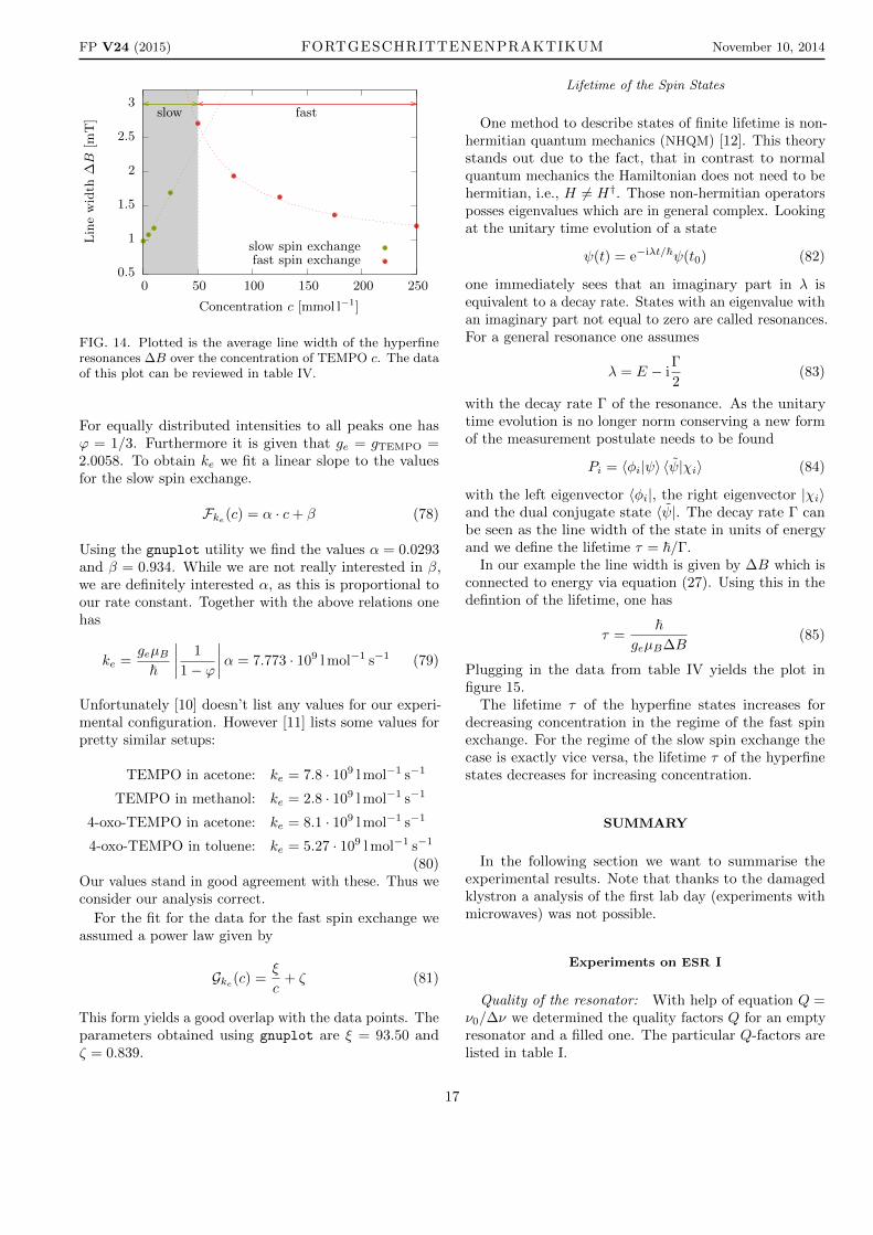
According to theory all line width should be the samefor the spectra with three peaks which they are almost ina first approximation. Still, to eliminate errors we averageover the values. The so obtained values are plotted overtheir corresponding concentration to achieve figure 14.The values for slow spin exchange are highlighted with agrey background. Even without the additional fit curvesone can clearly see that the values for slow spin exchangeare neatly aligned on an ascending slope, whereas thevalues for moderate and fast spin exchange obviouslydecay (it cannot be told at first sight if this is a powerlaw or an exponential).

In the basics, as in [10], a linear dependency betweenconcentration and line width was found for slow spinexchange.

kec =geµB~

∣∣∣∣ 1

1− ϕ

∣∣∣∣ (∆B(c)−∆B(0)) (77)

16


0.5

1

1.5

2

2.5

3

0 50 100 150 200 250

Lin

ew

idth

∆B

[mT

]

Concentration c [mmol l−1]

slow spin exchangefast spin exchange

slow fast

FIG. 14. Plotted is the average line width of the hyperfineresonances ∆B over the concentration of TEMPO c. The dataof this plot can be reviewed in table IV.

For equally distributed intensities to all peaks one hasϕ = 1/3. Furthermore it is given that ge = gTEMPO =2.0058. To obtain ke we fit a linear slope to the valuesfor the slow spin exchange.

Fke(c) = α · c+ β (78)

Using the gnuplot utility we find the values α = 0.0293and β = 0.934. While we are not really interested in β,we are definitely interested α, as this is proportional toour rate constant. Together with the above relations onehas

ke =geµB~

∣∣∣∣ 1

1− ϕ

∣∣∣∣α = 7.773 · 109 l mol−1 s−1 (79)

Unfortunately [10] doesn’t list any values for our experi-mental configuration. However [11] lists some values forpretty similar setups:

TEMPO in acetone: ke = 7.8 · 109 l mol−1 s−1

TEMPO in methanol: ke = 2.8 · 109 l mol−1 s−1

4-oxo-TEMPO in acetone: ke = 8.1 · 109 l mol−1 s−1

4-oxo-TEMPO in toluene: ke = 5.27 · 109 l mol−1 s−1

(80)Our values stand in good agreement with these. Thus weconsider our analysis correct.

For the fit for the data for the fast spin exchange weassumed a power law given by

Gke(c) =ξ

c+ ζ (81)

This form yields a good overlap with the data points. Theparameters obtained using gnuplot are ξ = 93.50 andζ = 0.839.

Lifetime of the Spin States

One method to describe states of finite lifetime is non-hermitian quantum mechanics (NHQM) [12]. This theorystands out due to the fact, that in contrast to normalquantum mechanics the Hamiltonian does not need to behermitian, i.e., H 6= H†. Those non-hermitian operatorsposses eigenvalues which are in general complex. Lookingat the unitary time evolution of a state

ψ(t) = e−iλt/~ψ(t0) (82)

one immediately sees that an imaginary part in λ isequivalent to a decay rate. States with an eigenvalue withan imaginary part not equal to zero are called resonances.For a general resonance one assumes

λ = E − iΓ

2(83)

with the decay rate Γ of the resonance. As the unitarytime evolution is no longer norm conserving a new formof the measurement postulate needs to be found

Pi = 〈φi|ψ〉〈ψ|χi〉 (84)

with the left eigenvector 〈φi|, the right eigenvector |χi〉and the dual conjugate state 〈ψ|. The decay rate Γ canbe seen as the line width of the state in units of energyand we define the lifetime τ = ~/Γ.

In our example the line width is given by ∆B which isconnected to energy via equation (27). Using this in thedefintion of the lifetime, one has

τ =~

geµB∆B(85)

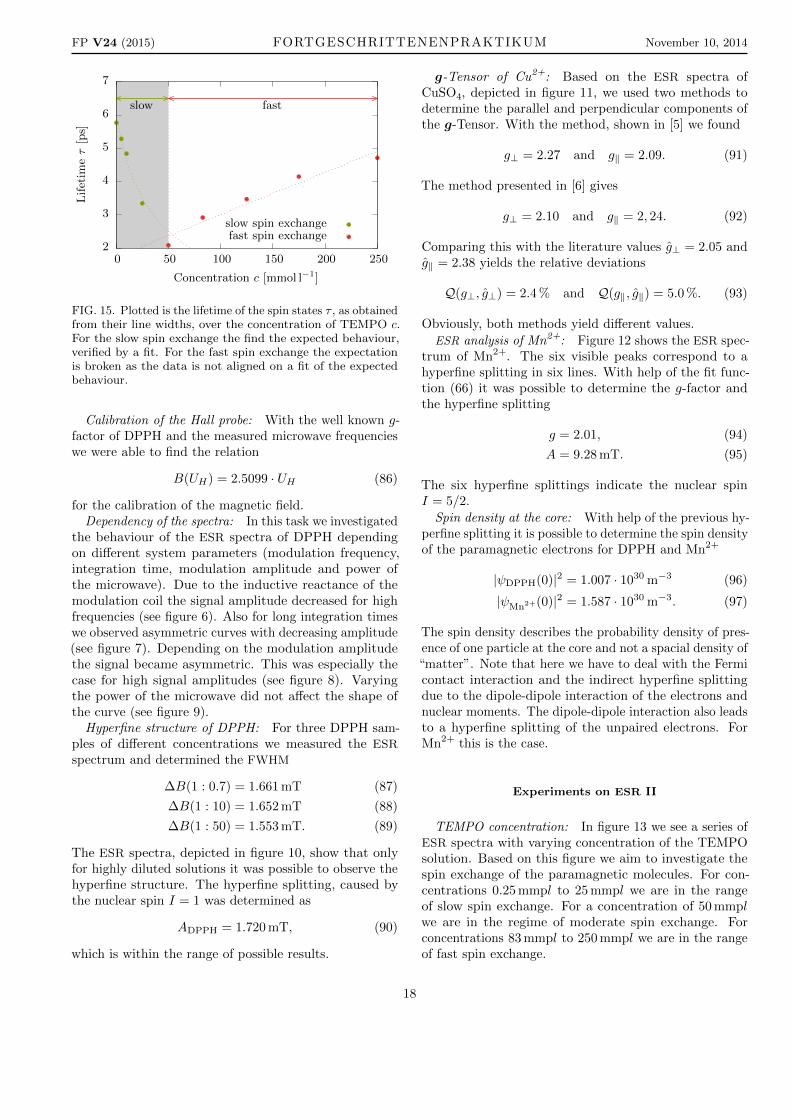
Plugging in the data from table IV yields the plot infigure 15.

The lifetime τ of the hyperfine states increases fordecreasing concentration in the regime of the fast spinexchange. For the regime of the slow spin exchange thecase is exactly vice versa, the lifetime τ of the hyperfinestates decreases for increasing concentration.

SUMMARY

In the following section we want to summarise theexperimental results. Note that thanks to the damagedklystron a analysis of the first lab day (experiments withmicrowaves) was not possible.

Experiments on ESR I

Quality of the resonator: With help of equation Q =ν0/∆ν we determined the quality factors Q for an emptyresonator and a filled one. The particular Q-factors arelisted in table I.

17


2

3

4

5

6

7

0 50 100 150 200 250

Lif

etim

eτ

[ps]

Concentration c [mmol l−1]

slow spin exchangefast spin exchange

slow fast

FIG. 15. Plotted is the lifetime of the spin states τ , as obtainedfrom their line widths, over the concentration of TEMPO c.For the slow spin exchange the find the expected behaviour,verified by a fit. For the fast spin exchange the expectationis broken as the data is not aligned on a fit of the expectedbehaviour.

Calibration of the Hall probe: With the well known g-factor of DPPH and the measured microwave frequencieswe were able to find the relation

B(UH) = 2.5099 · UH (86)

for the calibration of the magnetic field.Dependency of the spectra: In this task we investigated

the behaviour of the ESR spectra of DPPH dependingon different system parameters (modulation frequency,integration time, modulation amplitude and power ofthe microwave). Due to the inductive reactance of themodulation coil the signal amplitude decreased for highfrequencies (see figure 6). Also for long integration timeswe observed asymmetric curves with decreasing amplitude(see figure 7). Depending on the modulation amplitudethe signal became asymmetric. This was especially thecase for high signal amplitudes (see figure 8). Varyingthe power of the microwave did not affect the shape ofthe curve (see figure 9).

Hyperfine structure of DPPH: For three DPPH sam-ples of different concentrations we measured the ESR

spectrum and determined the FWHM

∆B(1 : 0.7) = 1.661 mT (87)

∆B(1 : 10) = 1.652 mT (88)

∆B(1 : 50) = 1.553 mT. (89)

The ESR spectra, depicted in figure 10, show that onlyfor highly diluted solutions it was possible to observe thehyperfine structure. The hyperfine splitting, caused bythe nuclear spin I = 1 was determined as

ADPPH = 1.720 mT, (90)

which is within the range of possible results.

g-Tensor of Cu2+: Based on the ESR spectra ofCuSO4, depicted in figure 11, we used two methods todetermine the parallel and perpendicular components ofthe g-Tensor. With the method, shown in [5] we found

g⊥ = 2.27 and g‖ = 2.09. (91)

The method presented in [6] gives

g⊥ = 2.10 and g‖ = 2, 24. (92)

Comparing this with the literature values g⊥ = 2.05 andg‖ = 2.38 yields the relative deviations

Q(g⊥, g⊥) = 2.4 % and Q(g‖, g‖) = 5.0 %. (93)

Obviously, both methods yield different values.

ESR analysis of Mn2+: Figure 12 shows the ESR spec-trum of Mn2+. The six visible peaks correspond to ahyperfine splitting in six lines. With help of the fit func-tion (66) it was possible to determine the g-factor andthe hyperfine splitting

g = 2.01, (94)

A = 9.28 mT. (95)

The six hyperfine splittings indicate the nuclear spinI = 5/2.

Spin density at the core: With help of the previous hy-perfine splitting it is possible to determine the spin densityof the paramagnetic electrons for DPPH and Mn2+

|ψDPPH(0)|2 = 1.007 · 1030 m−3 (96)

|ψMn2+(0)|2 = 1.587 · 1030 m−3. (97)

The spin density describes the probability density of pres-ence of one particle at the core and not a spacial density of“matter”. Note that here we have to deal with the Fermicontact interaction and the indirect hyperfine splittingdue to the dipole-dipole interaction of the electrons andnuclear moments. The dipole-dipole interaction also leadsto a hyperfine splitting of the unpaired electrons. ForMn2+ this is the case.

Experiments on ESR II

TEMPO concentration: In figure 13 we see a series ofESR spectra with varying concentration of the TEMPOsolution. Based on this figure we aim to investigate thespin exchange of the paramagnetic molecules. For con-centrations 0.25 mmpl to 25 mmpl we are in the rangeof slow spin exchange. For a concentration of 50 mmplwe are in the regime of moderate spin exchange. Forconcentrations 83 mmpl to 250 mmpl we are in the rangeof fast spin exchange.

18


Spin Exchange: Next, we plotted the average linewidth of the hyperfine resonances over the concentra-tions of TEMPO to determine the rate constant ke. Withhelp of equation 77 and an additional linear fit we found

ke = 7.773 · 109 l mol−1 s−1. (98)

which is within the range of possible results.Lifetime of the Spin States: In figure 15 the lifetime

of the spin states is plotted over the concentration ofTEMPO. With help of non-hermitian quantum mechanics(NHQM) we derived a term for the lifetime

τ =~

geµB∆B. (99)

The regime of slow spin exchange decreases form 6 ps to2.5 ps and transfer to the regime of fast spin exchange.Hence the lifetime τ decreases with increasing concentra-tion and vice versa for increasing τ .

APPENDIX

In this section you will find some formulas used in thereport which were not explained in the basics, becausethey are not related to ESR in any way. Furthermore youmay find comments on particular aspects of the reportwhich are not of scientific nature.

Arithmetic Mean: The arithmetic mean of a series isdefined as a sum over all members of the series dividedby the number of members. Let s = {si | 1 < i < N},then the arithmetic mean is given by

s ≡ 1

N

N∑i=1

si . (100)

Relative Deviation: The relative deviation is a measurefor the difference between two values and is given inpercent. Suppose a and b are measured values for thesame quantity and thus have the same unit. Their relativedeviation is given by

Q(a, b) =a− bb· 100 % . (101)

Constants: If not stated otherwise physical constantsare taken from [13].

∗ Michael [email protected]† [email protected]

[1] D. Meschede, Gerthsen Physik , 24th ed. (Springer Verlag,2007).

[2] W. Balter and L. W. Kroh, Schnellmethoden zurBeurteilung von Lebensmitteln und ihren Rohstoffen (Behr,2004).

[3] J. Davies, B. Gilbert, K. McLauchlan, and S. Eaton,Electron Paramagnetic Resonance, Specialist PeriodicalReports (Royal Society of Chemistry, 2000).

[4] R. W. Holmberg, A Paramagnetic Resonance Study ofHyperfine Interactions in Single Crystals Containing α,α-diphenyl-β-picrylhydrazyl., Tech. Rep. W-740.5-eng-26(Oak Ridge National Laboratories, 1961).

[5] F. K. Kneubuhl, The Journal of Chemical Physics 33,1074 (1960).

[6] R. D. Arnold and A. F. Kip, Phys. Rev. 75, 1199 (1949).[7] L. Turyanska, R. J. A. Hill, O. Makarovsky, F. Moro,

A. N. Knott, O. J. Larkin, A. Patane, A. Meaney, P. C. M.Christianen, M. W. Fay, and R. J. Curry, Nanoscale 6,8919 (2014).

[8] M. Zimmerman and N. Whitehead, New Applications ofElectron Spin Resonance: Dating, Dosimetry and Mi-croscopy (World Scientific, 1993).

[9] H. Haken and H. C. Wolf, Molekulphysik und Quanten-chemie, 5th ed. (Springer Verlag, 2005).

[10] Y. Molin, K. Salikhov, and K. Zamaraev, Spin Exchange:Principles and Applications in Chemistry and Biology,Springer Series in Chemical Physics (Springer Berlin Hei-delberg, 2012).

[11] G. Grampp and K. Rasmussen, Nitroxides – Theory, Ex-periment and Applications, (2012), 10.5772/39131.

[12] N. Moiseyev, Non-Hermitian Quantum Mechanics (Cam-bridge University Press, 2011).

[13] P. J. Mohr, B. N. Taylor, and D. B. Newell, Rev. Mod.Phys. 84, 1527 (2012).

19

Documents

o Electron Spin Resonance - Henri Menke Electron Spin Resonance Michael Schmid and Henri Menkey Gruppe M05, Fortgeschrittenenpraktikum, University of Stuttgart (November 10, 2014)