Embed Size (px)
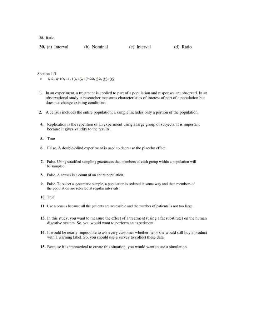
Citation preview
Section 1.1
o —1-10, 11, 13, 14, 17, 19, 21, 29, 30, 32, 33, 36, 38, 40, 41, 46, 47
CHAPTER
Introduction to Statistics
1 Copyright © 2012 Pearson Education, Inc. Publishing as Prentice Hall.
1
1.1 AN OVERVIEW OF STATISTICS 1.1 Try It Yourself Solutions 1a. The population consists of the prices per gallon of regular gasoline at all gasoline stations in the
United States. The sample consists of the prices per gallon of regular gasoline at the 900 surveyed stations.
b. The data set consists of the 900 prices. 2a. Because the numerical measure of $2,655,395,194 is based on the entire collection of player’s
salaries, it is from a population. b. Because the numerical measure is a characteristic of a population, it is a parameter. 3a. Descriptive statistics involve the statement “76% of women and 60% of men had a physical
examination within the previous year.” b. An inference drawn from the study is that a higher percentage of women had a physical
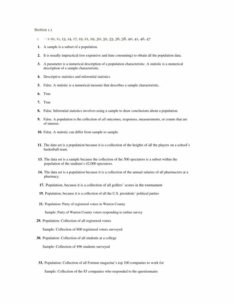
examination within the previous year. 1.1 EXERCISE SOLUTIONS 1. A sample is a subset of a population. 2. It is usually impractical (too expensive and time consuming) to obtain all the population data. 3. A parameter is a numerical description of a population characteristic. A statistic is a numerical
description of a sample characteristic. 4. Descriptive statistics and inferential statistics 5. False. A statistic is a numerical measure that describes a sample characteristic. 6. True 7. True 8. False. Inferential statistics involves using a sample to draw conclusions about a population. 9. False. A population is the collection of all outcomes, responses, measurements, or counts that are
of interest. 10. False. A statistic can differ from sample to sample. 2 CHAPTER 1 Ň INTRODUCTION TO STATISTICS
Copyright © 2012 Pearson Education, Inc. Publishing as Prentice Hall.
11. The data set is a population because it is a collection of the heights of all the players on a school’s basketball team.
12. The data set is a population because it is a collection of the energy collected from all the wind
turbines on the wind farm. 13. The data set is a sample because the collection of the 500 spectators is a subset within the
population of the stadium’s 42,000 spectators. 14. The data set is a population because it is a collection of the annual salaries of all pharmacists at a
pharmacy. 15. Sample, because the collection of the 20 patients is a subset within the population 16. The data set is a population since it is a collection of the number of televisions in all U.S.
households. 17. Population, because it is a collection of all golfers’ scores in the tournament 18. Sample, because only the age of every third person entering the clothing store is recorded 19. Population, because it is a collection of all the U.S. presidents’ political parties 20. Sample, because the collection of the 10 soil contamination levels is a subset in the population 21. Population: Party of registered voters in Warren County Sample: Party of Warren County voters responding to online survey 22. Population: All students who donate at a blood drive Sample: The students who donate and have type O+ blood 23. Population: Ages of adults in the United States who own cellular phones Sample: Ages of adults in the United States who own Samsung cellular phones 24. Population: Income of all homeowners in Texas Sample: Income of homeowners in Texas with mortgages 25. Population: Collection of all adults in the United States Sample: Collection of 1000 adults surveyed 26. Population: Collection of all infants in Italy Sample: Collection of 33,043 infants in the study
2 CHAPTER 1 Ň INTRODUCTION TO STATISTICS
Copyright © 2012 Pearson Education, Inc. Publishing as Prentice Hall.
11. The data set is a population because it is a collection of the heights of all the players on a school’s basketball team.
12. The data set is a population because it is a collection of the energy collected from all the wind
turbines on the wind farm. 13. The data set is a sample because the collection of the 500 spectators is a subset within the
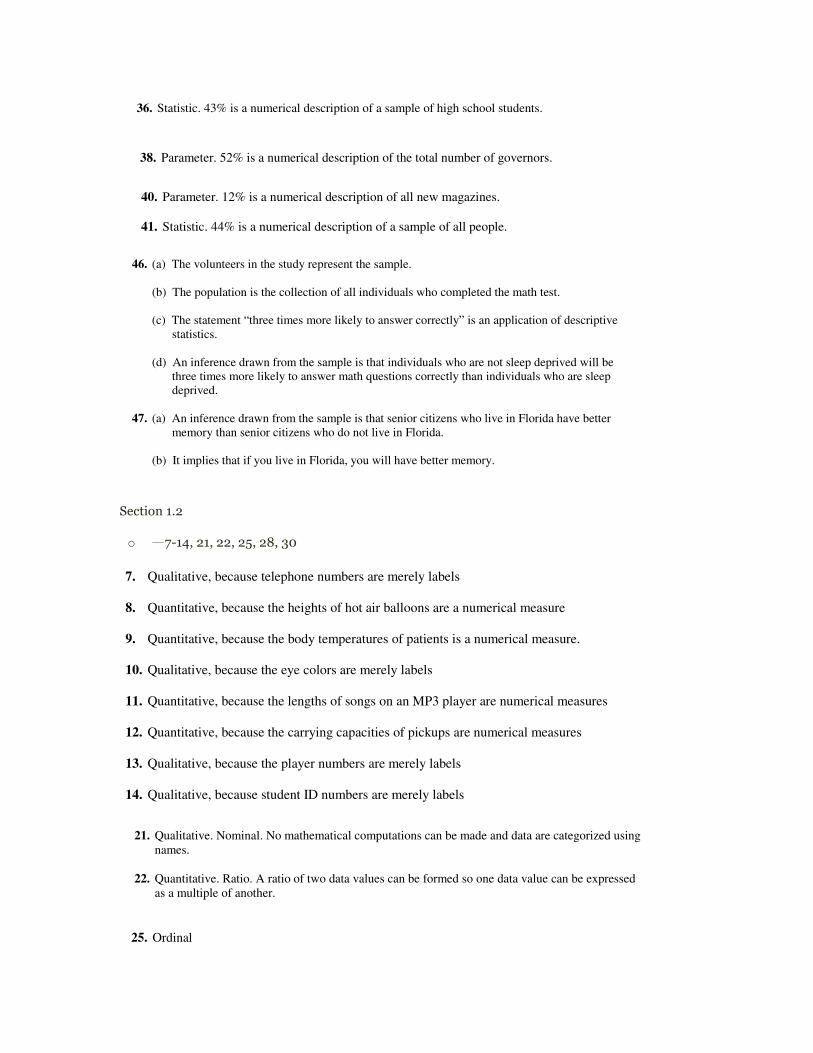
population of the stadium’s 42,000 spectators. 14. The data set is a population because it is a collection of the annual salaries of all pharmacists at a
pharmacy. 15. Sample, because the collection of the 20 patients is a subset within the population 16. The data set is a population since it is a collection of the number of televisions in all U.S.
households. 17. Population, because it is a collection of all golfers’ scores in the tournament 18. Sample, because only the age of every third person entering the clothing store is recorded 19. Population, because it is a collection of all the U.S. presidents’ political parties 20. Sample, because the collection of the 10 soil contamination levels is a subset in the population 21. Population: Party of registered voters in Warren County Sample: Party of Warren County voters responding to online survey 22. Population: All students who donate at a blood drive Sample: The students who donate and have type O+ blood 23. Population: Ages of adults in the United States who own cellular phones Sample: Ages of adults in the United States who own Samsung cellular phones 24. Population: Income of all homeowners in Texas Sample: Income of homeowners in Texas with mortgages 25. Population: Collection of all adults in the United States Sample: Collection of 1000 adults surveyed 26. Population: Collection of all infants in Italy Sample: Collection of 33,043 infants in the study
CHAPTER 1 Ň INTRODUCTION TO STATISTICS 3
Copyright © 2012 Pearson Education, Inc. Publishing as Prentice Hall.
27. Population: Collection of all adults in the U.S. Sample: Collection of 1442 adults surveyed 28. Population: Collection of all people Sample: Collection of 1600 people surveyed 29. Population: Collection of all registered voters Sample: Collection of 800 registered voters surveyed 30. Population: Collection of all students at a college Sample: Collection of 496 students surveyed 31. Population: Collection of all women in the U.S. Sample: Collection of the 546 U.S. women surveyed 32. Population: Collection of all U.S. vacationers Sample: Collection of the 791 vacationers surveyed 33. Population: Collection of all Fortune magazine’s top 100 companies to work for Sample: Collection of the 85 companies who responded to the questionnaire 34. Population: Collection of all light bulbs from the day’s production Sample: Collection of the 20 light bulbs selected from the day’s production 35. Statistic. The value $68,000 is a numerical description of a sample of annual salaries. 36. Statistic. 43% is a numerical description of a sample of high school students. 37. Parameter. The 62 surviving passengers out of 97 total passengers is a numerical description of
all of the passengers of the Hindenburg that survived. 38. Parameter. 52% is a numerical description of the total number of governors. 39. Statistic. 8% is a numerical description of a sample of computer users. 40. Parameter. 12% is a numerical description of all new magazines. 41. Statistic. 44% is a numerical description of a sample of all people. 42. Parameter. 21.0 is a numerical description of ACT scores for all graduates.
Section 1.2
o —7-14, 21, 22, 25, 28, 30
CHAPTER 1 Ň INTRODUCTION TO STATISTICS 3
Copyright © 2012 Pearson Education, Inc. Publishing as Prentice Hall.
27. Population: Collection of all adults in the U.S. Sample: Collection of 1442 adults surveyed 28. Population: Collection of all people Sample: Collection of 1600 people surveyed 29. Population: Collection of all registered voters Sample: Collection of 800 registered voters surveyed 30. Population: Collection of all students at a college Sample: Collection of 496 students surveyed 31. Population: Collection of all women in the U.S. Sample: Collection of the 546 U.S. women surveyed 32. Population: Collection of all U.S. vacationers Sample: Collection of the 791 vacationers surveyed 33. Population: Collection of all Fortune magazine’s top 100 companies to work for Sample: Collection of the 85 companies who responded to the questionnaire 34. Population: Collection of all light bulbs from the day’s production Sample: Collection of the 20 light bulbs selected from the day’s production 35. Statistic. The value $68,000 is a numerical description of a sample of annual salaries. 36. Statistic. 43% is a numerical description of a sample of high school students. 37. Parameter. The 62 surviving passengers out of 97 total passengers is a numerical description of
all of the passengers of the Hindenburg that survived. 38. Parameter. 52% is a numerical description of the total number of governors. 39. Statistic. 8% is a numerical description of a sample of computer users. 40. Parameter. 12% is a numerical description of all new magazines. 41. Statistic. 44% is a numerical description of a sample of all people. 42. Parameter. 21.0 is a numerical description of ACT scores for all graduates.
4 CHAPTER 1 Ň INTRODUCTION TO STATISTICS
Copyright © 2012 Pearson Education, Inc. Publishing as Prentice Hall.
43. The statement “56% are the primary investors in their household” is an application of descriptive statistics.
An inference drawn from the sample is that an association exists between U.S. women and being
the primary investor in their household. 44. The statement “spending at least $2000 for their next vacation” is an example of descriptive
statistics. An inference drawn from the sample is that United States vacationers are associated with
spending more than $2000 for their next vacation. 45. Answers will vary. 46. (a) The volunteers in the study represent the sample. (b) The population is the collection of all individuals who completed the math test. (c) The statement “three times more likely to answer correctly” is an application of descriptive
statistics. (d) An inference drawn from the sample is that individuals who are not sleep deprived will be
three times more likely to answer math questions correctly than individuals who are sleep deprived.
47. (a) An inference drawn from the sample is that senior citizens who live in Florida have better
memory than senior citizens who do not live in Florida. (b) It implies that if you live in Florida, you will have better memory. 48. (a) An inference drawn from the sample is that the obesity rate among boys ages 2 to 19 is
increasing. (b) It implies the same trend will continue in future years. 49. Answers will vary.
1.2 DATA CLASSIFICATION 1.2 Try It Yourself Solutions 1a. One data set contains names of cities and the other contains city populations. b. City: Nonnumerical Population: Numerical c. City: Qualitative Population: Quantitative
CHAPTER 1 Ň INTRODUCTION TO STATISTICS 5
Copyright © 2012 Pearson Education, Inc. Publishing as Prentice Hall.
2a. (1) The final standings represent a ranking of basketball teams. (2) The collection of phone numbers represents labels. No mathematical computations can be
made. b. (1) Ordinal, because the data can be put in order (2) Nominal, because you cannot make calculations on the data 3a. (1) The data set is the collection of body temperatures. (2) The data set is the collection of heart rates. b. (1) Interval, because the data can be ordered and meaningful differences can be calculated, but it
does not make sense writing a ratio using the temperatures (2) Ratio, because the data can be ordered, can be written as a ratio, you can calculate
meaningful differences, and the data set contains an inherent zero 1.2 EXERCISE SOLUTIONS 1. Nominal and ordinal 2. Ordinal, interval, and ratio 3. False. Data at the ordinal level can be qualitative or quantitative. 4. False. For data at the interval level, you can calculate meaningful differences between data
entries. You cannot calculate meaningful differences at the nominal or ordinal level. 5. False. More types of calculations can be performed with data at the interval level than with data at
the nominal level. 6. False. Data at the ratio level can be placed in a meaningful order. 7. Qualitative, because telephone numbers are merely labels 8. Quantitative, because the heights of hot air balloons are a numerical measure 9. Quantitative, because the body temperatures of patients is a numerical measure. 10. Qualitative, because the eye colors are merely labels 11. Quantitative, because the lengths of songs on an MP3 player are numerical measures 12. Quantitative, because the carrying capacities of pickups are numerical measures 13. Qualitative, because the player numbers are merely labels 14. Qualitative, because student ID numbers are merely labels
6 CHAPTER 1 Ň INTRODUCTION TO STATISTICS
Copyright © 2012 Pearson Education, Inc. Publishing as Prentice Hall.
15. Quantitative, because weights of infants are a numerical measure 16. Qualitative, because species of trees are merely labels 17. Qualitative, because the poll results are merely responses 18. Quantitative, because wait times at a grocery store are a numerical measure 19. Qualitative. Ordinal. Data can be arranged in order, but differences between data entries make no
sense. 20. Qualitative. Nominal. No mathematical computations can be made and data are categorized using
names. 21. Qualitative. Nominal. No mathematical computations can be made and data are categorized using
names. 22. Quantitative. Ratio. A ratio of two data values can be formed so one data value can be expressed
as a multiple of another. 23. Qualitative. Ordinal. The data can be arranged in order, but differences between data entries are
not meaningful. 24. Quantitative. Ratio. The ratio of two data values can be formed so one data value can be
expressed as a multiple of another. 25. Ordinal 26. Ratio 27. Nominal 28. Ratio 29. (a) Interval (b) Nominal (c) Ratio (d) Ordinal 30. (a) Interval (b) Nominal (c) Interval (d) Ratio 31. An inherent zero is a zero that implies “none.” Answers will vary. 32. Answers will vary.
1.3 DATA COLLECTION AND EXPERIMENTAL DESIGN 1.3 Try It Yourself Solutions 1a. (1) Focus: Effect of exercise on relieving depression (2) Focus: Success of graduates
Section 1.3 o 1, 2, 4-10, 11, 13, 15, 17-22, 32, 33, 35
6 CHAPTER 1 Ň INTRODUCTION TO STATISTICS
Copyright © 2012 Pearson Education, Inc. Publishing as Prentice Hall.
15. Quantitative, because weights of infants are a numerical measure 16. Qualitative, because species of trees are merely labels 17. Qualitative, because the poll results are merely responses 18. Quantitative, because wait times at a grocery store are a numerical measure 19. Qualitative. Ordinal. Data can be arranged in order, but differences between data entries make no
sense. 20. Qualitative. Nominal. No mathematical computations can be made and data are categorized using
names. 21. Qualitative. Nominal. No mathematical computations can be made and data are categorized using
names. 22. Quantitative. Ratio. A ratio of two data values can be formed so one data value can be expressed
as a multiple of another. 23. Qualitative. Ordinal. The data can be arranged in order, but differences between data entries are
not meaningful. 24. Quantitative. Ratio. The ratio of two data values can be formed so one data value can be
expressed as a multiple of another. 25. Ordinal 26. Ratio 27. Nominal 28. Ratio 29. (a) Interval (b) Nominal (c) Ratio (d) Ordinal 30. (a) Interval (b) Nominal (c) Interval (d) Ratio 31. An inherent zero is a zero that implies “none.” Answers will vary. 32. Answers will vary.
1.3 DATA COLLECTION AND EXPERIMENTAL DESIGN 1.3 Try It Yourself Solutions 1a. (1) Focus: Effect of exercise on relieving depression (2) Focus: Success of graduates
CHAPTER 1 Ň INTRODUCTION TO STATISTICS 7
Copyright © 2012 Pearson Education, Inc. Publishing as Prentice Hall.
b. (1) Population: Collection of all people with depression (2) Population: Collection of all university graduates at this large university c. (1) Experiment (2) Survey 2a. There is no way to tell why people quit smoking. They could have quit smoking either from the
gum or from watching the DVD. b. Two experiments could be done; one using the gum and the other using the DVD. 3a. Example: start with the first digits 92630782 … b. 92 63 07 82 40 19 26 c. 63, 7, 40, 19, 26 4a. (1) The sample was selected by only using the students in a randomly chosen class. Cluster
sampling (2) The sample was selected by numbering each student in the school, randomly choosing a
starting number, and selecting students at regular intervals from the starting number. Systematic sampling
b. (1) The sample may be biased because some classes may be more familiar with stem cell
research than other classes and have stronger opinions. (2) The sample may be biased if there is any regularly occurring pattern in the data. 1.3 EXERCISE SOLUTIONS 1. In an experiment, a treatment is applied to part of a population and responses are observed. In an
observational study, a researcher measures characteristics of interest of part of a population but does not change existing conditions.
2. A census includes the entire population; a sample includes only a portion of the population. 3. In a random sample, every member of the population has an equal chance of being selected. In a
simple random sample, every possible sample of the same size has an equal chance of being selected.
4. Replication is the repetition of an experiment using a large group of subjects. It is important
because it gives validity to the results. 5. True 6. False. A double-blind experiment is used to decrease the placebo effect.
CHAPTER 1 Ň INTRODUCTION TO STATISTICS 7
Copyright © 2012 Pearson Education, Inc. Publishing as Prentice Hall.
b. (1) Population: Collection of all people with depression (2) Population: Collection of all university graduates at this large university c. (1) Experiment (2) Survey 2a. There is no way to tell why people quit smoking. They could have quit smoking either from the
gum or from watching the DVD. b. Two experiments could be done; one using the gum and the other using the DVD. 3a. Example: start with the first digits 92630782 … b. 92 63 07 82 40 19 26 c. 63, 7, 40, 19, 26 4a. (1) The sample was selected by only using the students in a randomly chosen class. Cluster
sampling (2) The sample was selected by numbering each student in the school, randomly choosing a
starting number, and selecting students at regular intervals from the starting number. Systematic sampling
b. (1) The sample may be biased because some classes may be more familiar with stem cell
research than other classes and have stronger opinions. (2) The sample may be biased if there is any regularly occurring pattern in the data. 1.3 EXERCISE SOLUTIONS 1. In an experiment, a treatment is applied to part of a population and responses are observed. In an
observational study, a researcher measures characteristics of interest of part of a population but does not change existing conditions.
2. A census includes the entire population; a sample includes only a portion of the population. 3. In a random sample, every member of the population has an equal chance of being selected. In a
simple random sample, every possible sample of the same size has an equal chance of being selected.
4. Replication is the repetition of an experiment using a large group of subjects. It is important
because it gives validity to the results. 5. True 6. False. A double-blind experiment is used to decrease the placebo effect. 8 CHAPTER 1 Ň INTRODUCTION TO STATISTICS
Copyright © 2012 Pearson Education, Inc. Publishing as Prentice Hall.
7. False. Using stratified sampling guarantees that members of each group within a population will be sampled.
8. False. A census is a count of an entire population. 9. False. To select a systematic sample, a population is ordered in some way and then members of
the population are selected at regular intervals. 10. True 11. Use a census because all the patients are accessible and the number of patients is not too large. 12. Perform an observational study because you want to observe and record motorcycle helmet usage. 13. In this study, you want to measure the effect of a treatment (using a fat substitute) on the human
digestive system. So, you would want to perform an experiment. 14. It would be nearly impossible to ask every customer whether he or she would still buy a product
with a warning label. So, you should use a survey to collect these data. 15. Because it is impractical to create this situation, you would want to use a simulation. 16. Perform an observational study because you want to observe and record how often people wash
their hands in public restrooms. 17. (a) The experimental units are the 30–35 year old females being given the treatment. One
treatment is used. (b) A problem with the design is that there may be some bias on the part of the researchers if he
or she knows which patients were given the real drug. A way to eliminate this problem would be to make the study into a double-blind experiment.
(c) The study would be a double-blind study if the researcher did not know which patients
received the real drug or the placebo. 18. (a) The experimental units are the 80 people with early signs of arthritis. One treatment is used. (b) A problem with the design is that the sample size is small. The experiment could be
replicated to increase validity. (c) In a placebo-controlled double-blind experiment, neither the subject nor the experimenter
knows whether the subject is receiving a treatment or a placebo. The experimenter is informed after all the data have been collected.
(d) The group could be randomly split into 20 males or 20 females in each treatment group. 19. Each U.S. telephone number has an equal chance of being dialed and all samples of 1400 phone
numbers have an equal chance of being selected, so this is a simple random sample. Telephone sampling only samples those individuals who have telephones, are available, and are willing to respond, so this is a possible source of bias.
8 CHAPTER 1 Ň INTRODUCTION TO STATISTICS
Copyright © 2012 Pearson Education, Inc. Publishing as Prentice Hall.
7. False. Using stratified sampling guarantees that members of each group within a population will be sampled.
8. False. A census is a count of an entire population. 9. False. To select a systematic sample, a population is ordered in some way and then members of
the population are selected at regular intervals. 10. True 11. Use a census because all the patients are accessible and the number of patients is not too large. 12. Perform an observational study because you want to observe and record motorcycle helmet usage. 13. In this study, you want to measure the effect of a treatment (using a fat substitute) on the human
digestive system. So, you would want to perform an experiment. 14. It would be nearly impossible to ask every customer whether he or she would still buy a product
with a warning label. So, you should use a survey to collect these data. 15. Because it is impractical to create this situation, you would want to use a simulation. 16. Perform an observational study because you want to observe and record how often people wash
their hands in public restrooms. 17. (a) The experimental units are the 30–35 year old females being given the treatment. One
treatment is used. (b) A problem with the design is that there may be some bias on the part of the researchers if he
or she knows which patients were given the real drug. A way to eliminate this problem would be to make the study into a double-blind experiment.
(c) The study would be a double-blind study if the researcher did not know which patients
received the real drug or the placebo. 18. (a) The experimental units are the 80 people with early signs of arthritis. One treatment is used. (b) A problem with the design is that the sample size is small. The experiment could be
replicated to increase validity. (c) In a placebo-controlled double-blind experiment, neither the subject nor the experimenter
knows whether the subject is receiving a treatment or a placebo. The experimenter is informed after all the data have been collected.
(d) The group could be randomly split into 20 males or 20 females in each treatment group. 19. Each U.S. telephone number has an equal chance of being dialed and all samples of 1400 phone
numbers have an equal chance of being selected, so this is a simple random sample. Telephone sampling only samples those individuals who have telephones, are available, and are willing to respond, so this is a possible source of bias.
CHAPTER 1 Ň INTRODUCTION TO STATISTICS 9
Copyright © 2012 Pearson Education, Inc. Publishing as Prentice Hall.
20. Because the persons are divided into strata (rural and urban), and a sample is selected from each stratum, this is a stratified sample.
21. Because the students were chosen due to their convenience of location (leaving the library), this is
a convenience sample. Bias may enter into the sample because the students sampled may not be representative of the population of students. For example, there may be an association between time spent at the library and drinking habits.
22. Because the disaster area was divided into grids and thirty grids were then entirely selected, this
is a cluster sample. Certain grids may have been much more severely damaged than others, so this is a possible source of bias.
23. Simple random sampling is used because each customer has an equal chance of being contacted,
and all samples of 580 customers have an equal chance of being selected. 24. Systematic sampling is used because every tenth person entering the shopping mall is sampled. It
is possible for bias to enter the sample if, for some reason, there is a regular pattern to people entering the shopping mall.
25. Because a sample is taken from each one-acre subplot (stratum), this is a stratified sample. 26. Each telephone has an equal chance of being dialed and all samples of 1012 phone numbers have
an equal chance of being selected, so this is a simple random sample. Telephone sampling only samples those individuals who have telephones and are willing to respond, so this is a possible source of bias.
27. Answers will vary. 28. Answers will vary. 29. Answers will vary. 30. Answers will vary. 31. Census, because it is relatively easy to obtain the ages of the 115 residents 32. Sampling, because the population of subscribers is too large to easily record their favorite movie
type. Random sampling would be advised since it would be too easy to randomly select subscribers then record their favorite movie type.
33. Question is biased because it already suggests that eating whole-grain foods is good for you. The
question might be rewritten as “How does eating whole-grain foods affect your health?” 34. Question is biased because it already suggests that text messaging while driving increases the risk
of a crash. The question might be rewritten as “Does text messaging while driving increase the risk of a crash?”
35. Question is unbiased because it does not imply how much exercise is good or bad.
Section 2.1—
o 1, 2, 3, 21, 25, 34, 37
CHAPTER 2 Ň DESCRIPTIVE STATISTICS 17
Copyright © 2012 Pearson Education, Inc. Publishing as Prentice Hall.
5abc.
6a. Use upper class boundaries for the horizontal scale and cumulative frequency for the vertical
scale. b. See part (c). c.
d. Approximately 40 of the 50 richest people are 80 years or younger. e. Answers will vary. 7ab.
2.1 EXERCISE SOLUTIONS 1. Organizing the data into a frequency distribution may make patterns within the data more evident.
Sometimes it is easier to identify patterns of a data set by looking at a graph of the frequency distribution.
2. If there are too few or too many classes, it may be difficult to detect patterns because the data are
too condensed or too spread out. 3. Class limits determine which numbers can belong to that class. Class boundaries are the numbers that separate classes without forming gaps between them.
20 CHAPTER 2 Ň DESCRIPTIVE STATISTICS
Copyright © 2012 Pearson Education, Inc. Publishing as Prentice Hall.
19a. Number of classes = 7 b. Least frequency 10 c. Greatest frequency 300 d. Class width = 10 20a. Number of classes = 7 b. Least frequency 100 c. Greatest frequency 900 d. Class width = 5 21a. 50 b. 22.5-23.5 pounds 22a. 50 b. 64-66 inches 23a. 42 b. 29.5 pounds c. 35 d. 2 24a. 48 b. 66 inches c. 20 d. 6 25a. Class with greatest relative frequency: 8-9 inches Class with least relative frequency: 17-18 inches b. Greatest relative frequency 0.195 Least relative frequency 0.005 c. Approximately 0.015 26a. Class with greatest relative frequency: 19-20 minutes Class with least relative frequency: 21-22 minutes b. Greatest relative frequency 40% Least relative frequency 2% c. Approximately 33% 27. Class with greatest frequency: 29.5-32.5 Classes with least frequency: 11.5-14.5 and 38.5-41.5 28. Class with greatest frequency: 7.75-8.25 Class with least frequency: 6.25-6.75
29. Class width = Range
Number of classes =
39 05�
= 7.8 8º
Class Frequency, f Midpoint Relative frequency
Cumulative frequency
0-7 8 3.5 0.32 8 8-15 8 11.5 0.32 16 16-23 3 19.5 0.12 19 24-31 3 27.5 0.12 22 32-39 3 35.5 0.12 25
25f �� 1fn��
Classes with greatest frequency: 0-7, 8-15 Classes with least frequency: 16-23, 24-31, 32-39
22 CHAPTER 2 Ň DESCRIPTIVE STATISTICS
Copyright © 2012 Pearson Education, Inc. Publishing as Prentice Hall.
The graph shows that most of the pungencies of the peppers were between 36 and 43 Scoville
units. (Answers will vary.)
33. Class width = Range
Number of classes =
514 2918�
= 27.875 28º
Class Frequency, f Midpoint Relative frequency
Cumulative frequency
291-318 5 304.5 0.1667 5 319-346 4 332.5 0.1333 9 347-374 3 360.5 0.1000 12 375-402 5 388.5 0.1667 17 403-430 6 416.5 0.2000 23 431-458 4 444.5 0.1333 27 459-486 1 472.5 0.0333 28 487-514 2 500.5 0.0667 30
30f �� 1fn��
The graph shows that the most frequent reaction times were between 403 and 430 milliseconds.
(Answers will vary.)
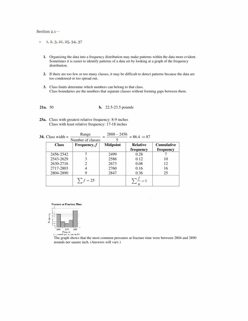
34. Class width = Range
Number of classes =
2888 24565�
= 86.4 87º
Class Frequency, f Midpoint Relative frequency
Cumulative frequency
2456-2542 7 2499 0.28 7 2543-2629 3 2586 0.12 10 2630-2716 2 2673 0.08 12 2717-2803 4 2760 0.16 16 2804-2890 9 2847 0.36 25
25f �� 1fn��
CHAPTER 2 Ň DESCRIPTIVE STATISTICS 23
Copyright © 2012 Pearson Education, Inc. Publishing as Prentice Hall.
The graph shows that the most common pressures at fracture time were between 2804 and 2890
pounds per square inch. (Answers will vary.)
35. Class width = Range
Number of classes =
55 245�
= 6.2 7º
Class Frequency, f Midpoint Relative frequency
Cumulative frequency
24-30 9 27 0.30 9 31-37 8 34 0.27 17 38-44 10 41 0.33 27 45-51 2 48 0.07 29 52-58 1 55 0.03 30
30f �� 1fn��
Class with greatest relative frequency: 38-44 Class with least relative frequency: 52-58
36. Class width = Range
Number of classes =
80 105�
= 14 15º
Class Frequency, f Midpoint Relative frequency
Cumulative frequency
10-24 11 17 0.3438 11 25-39 9 32 0.2813 20 40-54 6 47 0.1875 26 55-69 2 62 0.0625 28 70-84 4 77 0.1250 32
32f �� 1fnx�

Section 2.2
o 1, 5-8, 17, 23, 30, 34, 35-38
24 CHAPTER 2 Ň DESCRIPTIVE STATISTICS
Copyright © 2012 Pearson Education, Inc. Publishing as Prentice Hall.
Class with greatest relative frequency: 10-24 Class with least relative frequency: 55-69
37. Class width = Range
Number of classes =
462 1385�
= 64.8 65º
Class Frequency, f Midpoint Relative frequency
Cumulative frequency
138-202 12 170 0.46 12 203-267 6 235 0.23 18 268-332 4 300 0.15 22 333-397 1 365 0.04 23 398-462 3 430 0.12 26
26f �� 1fn��
Class with greatest relative frequency: 138-202 Class with least relative frequency: 333-397
38. Class width = Range
Number of classes =
14 65�
= 1.6 2º
Class Frequency, f Midpoint Relative frequency
Cumulative frequency
6-7 3 6.5 0.12 3 8-9 10 8.5 0.38 13
10-11 6 10.5 0.23 19 12-13 6 12.5 0.23 25 14-15 1 14.5 0.04 26
26f �� 1fn��
32 CHAPTER 2 Ň DESCRIPTIVE STATISTICS
Copyright © 2012 Pearson Education, Inc. Publishing as Prentice Hall.
5a. Cause Frequency, f Auto Dealers 14,668 Auto Repair 9,728 Home Furnishing 7,792 Computer Sales 5,733 Dry Cleaning 4,649
b.
c. It appears that the auto industry (dealers and repair shops) account for the largest portion of
complaints filed at the BBB. (Answers will very.) 6a, b.
c. It appears that the longer an employee is with the company, the larger the employee’s salary will
be. 7a, b.
c. The average bill increased from 1998 to 2004, then it hovered around $50.00 from 2004 to 2008. 2.2 EXERCISE SOLUTIONS 1. Quantitative: stem-and-leaf plot, dot plot, histogram, time series chart, scatter plot. Qualitative: pie chart, Pareto chart 2. Unlike the histogram, the stem-and-leaf plot still contains the original data values. However,
some data are difficult to organize in a stem-and-leaf plot.
CHAPTER 2 Ň DESCRIPTIVE STATISTICS 33
Copyright © 2012 Pearson Education, Inc. Publishing as Prentice Hall.
3. Both the stem-and-leaf plot and the dot plot allow you to see how data are distributed, determine specific data entries, and identify unusual data values.
4. In a Pareto chart, the height of each bar represents frequency or relative frequency and the bars
are positioned in order of decreasing height with the tallest bar positioned at the left. 5. b 6. d 7. a 8. c 9. 27, 32, 41, 43, 43, 44, 47, 47, 48, 50, 51, 51, 52, 53, 53, 53, 54, 54, 54, 54, 55, 56, 56, 58, 59, 68,
68, 68, 73, 78, 78, 85 Max: 85 Min: 27 10. 12.9, 13.3, 13.6, 13.7, 13.7, 14.1, 14.1, 14.1, 14.1, 14.3, 14.4, 14.4, 14.6, 14.9, 14.9, 15.0, 15.0,
15.0, 15.1, 15.2, 15.4, 15.6, 15.7, 15.8, 15.8, 15.8, 15.9, 16.1, 16.6, 16.7 Max: 16.7 Min: 12.9 11. 13, 13, 14, 14, 14, 15, 15, 15, 15, 15, 16, 17, 17, 18, 19 Max: 19 Min: 13 12. 214, 214, 214, 216, 216, 217, 218, 218, 220, 221, 223, 224, 225, 225, 227, 228, 228, 228, 228,
230, 230, 231, 235, 237, 239 Max: 239 Min: 214 13. Sample answer: Users spend the most amount of time on MySpace and the least amount of time
on Twitter. Answers will vary. 14. Sample answer: Motor vehicle thefts decreased between 2003 and 2008. Answers will vary. 15. Answers will vary. Sample answer: Tailgaters irk drivers the most, while too cautious drivers irk
drivers the least. 16. Answers will vary. Sample answer: The most frequent incident occurring while driving and using
a cell phone is swerving. Twice as many people “sped up” than “cut off a car.” 17. Key: 6 7 67�
6 7 8
7 3 5 5 6 9
0 0 2 3 5 5 7 7 88
0 1 1 1 2 4 5 59
It appears that most grades for the biology midterm were in the 80s or 90s. (Answers will vary.)
CHAPTER 2 Ň DESCRIPTIVE STATISTICS 35
Copyright © 2012 Pearson Education, Inc. Publishing as Prentice Hall.
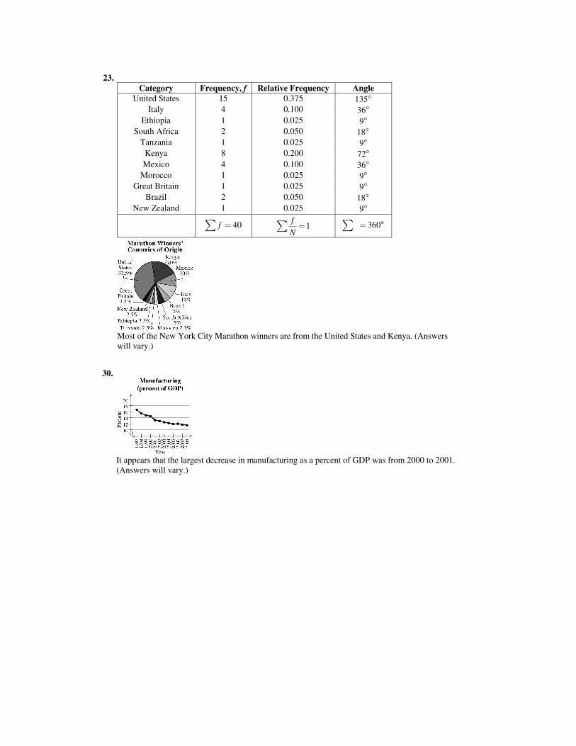
23. Category Frequency, f Relative Frequency Angle
United States 15 0.375 135n Italy 4 0.100 36n
Ethiopia 1 0.025 9n South Africa 2 0.050 18n
Tanzania 1 0.025 9n Kenya 8 0.200 72n Mexico 4 0.100 36n
Morocco 1 0.025 9n Great Britain 1 0.025 9n
Brazil 2 0.050 18n New Zealand 1 0.025 9n
40f �� 1fN
�� 360� n�
Most of the New York City Marathon winners are from the United States and Kenya. (Answers
will vary.) 24.
Category Frequency, f Relative Frequency Angle Science, aeronautics, exploration 8947 0.479 172.4n
Space operations 6176 0.331 119.2n Education 126 0.007 2.5n
Cross-agency support 3401 0.182 65.5n Inspector general 36 0.002 0.7n
18,686f �� 1fN
x� 360x n�
It appears that most of NASA’s budget was spent on science, aeronautics, and exploration.
(Answers will vary.)
CHAPTER 2 Ň DESCRIPTIVE STATISTICS 37
Copyright © 2012 Pearson Education, Inc. Publishing as Prentice Hall.
29.
It appears that it was hottest from May 7 to May 11. (Answers will vary.) 30.
It appears that the largest decrease in manufacturing as a percent of GDP was from 2000 to 2001.
(Answers will vary.) 31. Variable: Scores Key: 5 5 5.5�
5 5
6 2
6 8
7 0 1
7 5 6
0 2 38
5 6 7 8 8 98
0 3 39
5 5 8 99
010
It appears that most scores on the final exam in economics were in the 80’s and 90’s. (Answers will vary.)
CHAPTER 2 Ň DESCRIPTIVE STATISTICS 39
Copyright © 2012 Pearson Education, Inc. Publishing as Prentice Hall.
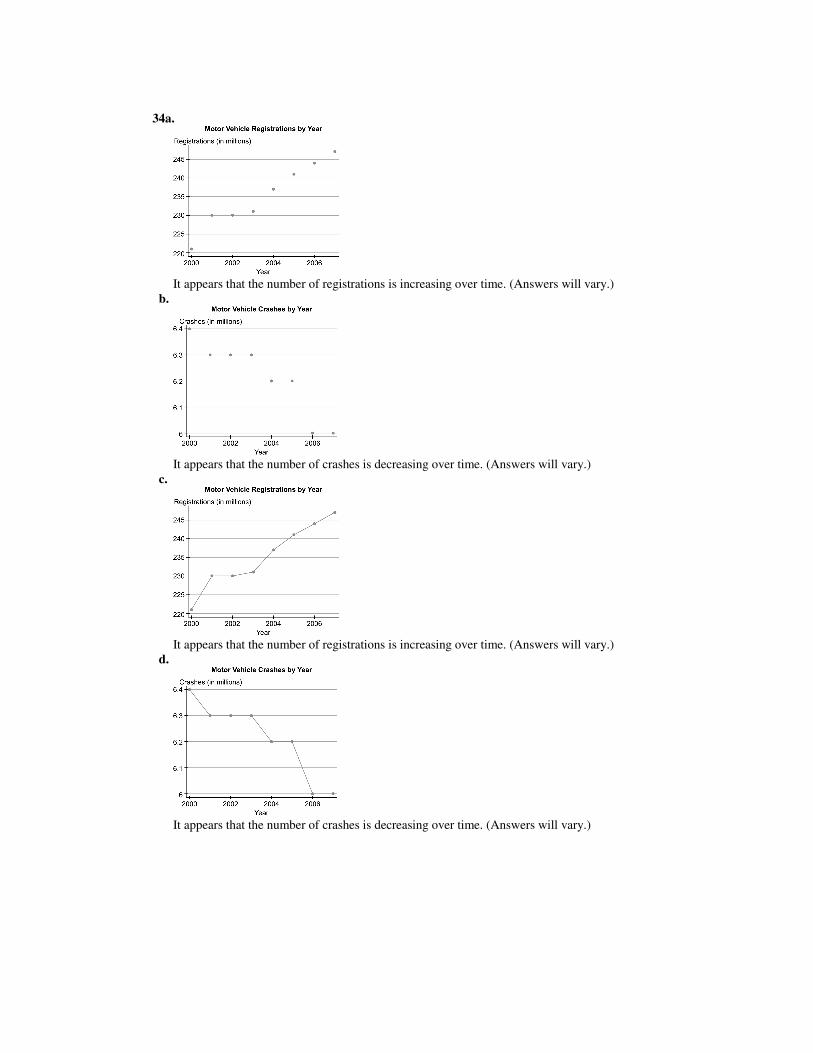
34a.
It appears that the number of registrations is increasing over time. (Answers will vary.) b.
It appears that the number of crashes is decreasing over time. (Answers will vary.) c.
It appears that the number of registrations is increasing over time. (Answers will vary.) d.
It appears that the number of crashes is decreasing over time. (Answers will vary.)
40 CHAPTER 2 Ň DESCRIPTIVE STATISTICS
Copyright © 2012 Pearson Education, Inc. Publishing as Prentice Hall.
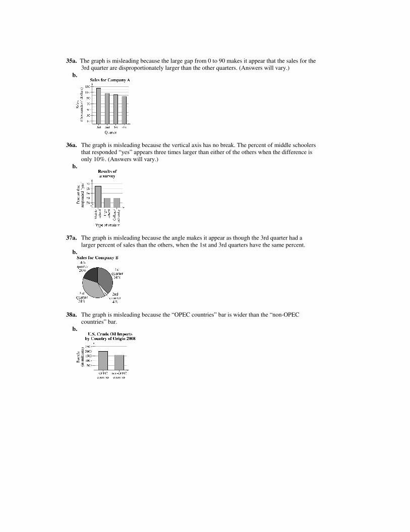
35a. The graph is misleading because the large gap from 0 to 90 makes it appear that the sales for the 3rd quarter are disproportionately larger than the other quarters. (Answers will vary.)
b.
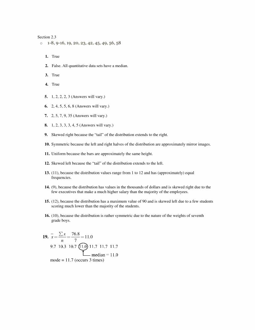
36a. The graph is misleading because the vertical axis has no break. The percent of middle schoolers
that responded “yes” appears three times larger than either of the others when the difference is only 10%. (Answers will vary.)
b.
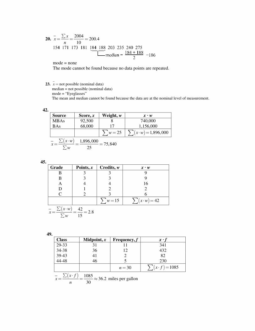
37a. The graph is misleading because the angle makes it appear as though the 3rd quarter had a
larger percent of sales than the others, when the 1st and 3rd quarters have the same percent. b.
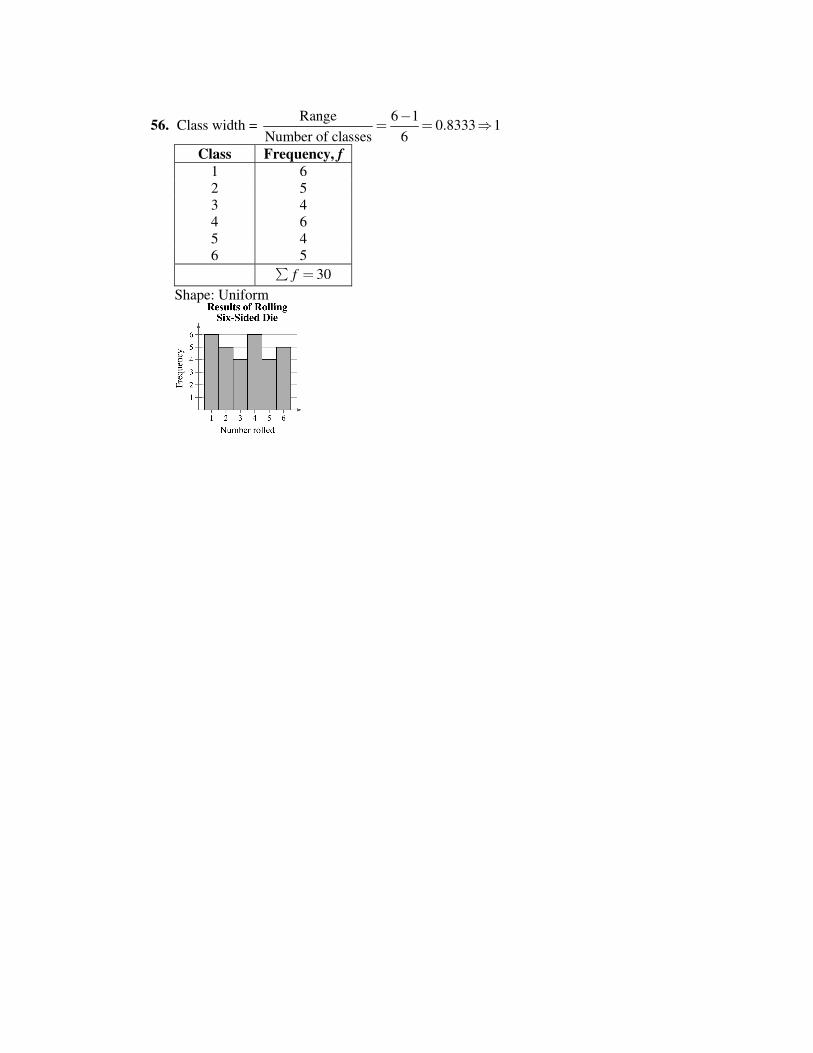
38a. The graph is misleading because the “OPEC countries” bar is wider than the “non-OPEC
countries” bar. b.
39a. At Law Firm A, the lowest salary was $90,000 and the highest salary was $203,000. At Law
Firm B, the lowest salary was $90,000 and the highest salary was $190,000. b. There are 30 lawyers at Law Firm A and 32 lawyers at Law Firm B.
Section 2.3 o 1-8, 9-16, 19, 20, 23, 42, 45, 49, 56, 58
42 CHAPTER 2 Ň DESCRIPTIVE STATISTICS
Copyright © 2012 Pearson Education, Inc. Publishing as Prentice Hall.
b. The mode of the responses to the survey is “Yes.” In this sample, there were more people who thought public cell phone conversations were rude than people who did not or had no opinion.
6a. 410
21.619
xx
n�
� � x
median = 21 mode = 20 b. The mean in Example 6 ( 23.8x x ) was heavily influenced by the entry 65. Neither the median
nor the mode was affected as much by the entry 65. 7a, b.
Source Score, x Weight, w x · w Test mean 86 0.50 43.0 Midterm 96 0.15 14.4 Final exam 98 0.20 19.6 Computer lab 98 0.10 9.8 Homework 100 0.05 5.0 1w�� 91.8x w¸ ��
c. 91.8
91.81
x wx
w
� ¸� � �
�
d. The weighted mean for the course is 91.8. So, you did get an A. 8a, b, c.
Class Midpoint, x Frequency, f x · f 35-41 38 2 76 42-48 45 5 225 49-55 52 7 364 56-62 59 7 413 63-69 66 10 660 70-76 73 5 365 77-83 80 8 640 84-90 87 6 552
N = 50 3265x f¸ ��
d. 3265
65.350
x f
NN
� ¸� � �
The mean age of the 50 richest people is 65.3 2.3 EXERCISE SOLUTIONS 1. True 2. False. All quantitative data sets have a median. 3. True 4. True
CHAPTER 2 Ň DESCRIPTIVE STATISTICS 43
Copyright © 2012 Pearson Education, Inc. Publishing as Prentice Hall.
5. 1, 2, 2, 2, 3 (Answers will vary.) 6. 2, 4, 5, 5, 6, 8 (Answers will vary.) 7. 2, 5, 7, 9, 35 (Answers will vary.) 8. 1, 2, 3, 3, 3, 4, 5 (Answers will vary.) 9. Skewed right because the “tail” of the distribution extends to the right. 10. Symmetric because the left and right halves of the distribution are approximately mirror images. 11. Uniform because the bars are approximately the same height. 12. Skewed left because the “tail” of the distribution extends to the left. 13. (11), because the distribution values range from 1 to 12 and has (approximately) equal
frequencies. 14. (9), because the distribution has values in the thousands of dollars and is skewed right due to the
few executives that make a much higher salary than the majority of the employees. 15. (12), because the distribution has a maximum value of 90 and is skewed left due to a few students
scoring much lower than the majority of the students. 16. (10), because the distribution is rather symmetric due to the nature of the weights of seventh
grade boys.
17. 64
4.913
xx
n�
� � x
mode = 4 (occurs 3 times)
18. 396
39.610
xx
n�
� � �
mode = 39 (occurs 3 times)
19. 76.8
11.07
xx
n�
� � �
mode = 11.7 (occurs 3 times)
44 CHAPTER 2 Ň DESCRIPTIVE STATISTICS
Copyright © 2012 Pearson Education, Inc. Publishing as Prentice Hall.
20. 2004
200.410
xx
n�
� � �
mode = none The mode cannot be found because no data points are repeated.
21. 686.8
21.4632
xx
n�
� � �
mode = 20.4 (occurs 2 times)
22. 1223
61.220
xx
n�
� � �
mode = 80, 125 The modes do not represent the center of the data set because they are large values compared to
the rest of the data. 23. x � not possible (nominal data) median = not possible (nominal data) mode = “Eyeglasses” The mean and median cannot be found because the data are at the nominal level of measurement. 24. x � not possible (nominal data) median = not possible (nominal data) mode = “Money needed” The mean and median cannot be found because the data are at the nominal level of measurement.
25. 1194.4
170.637
xx
n�
� � x
mode = none The mode cannot be found because no data points are repeated. 26. x � not possible (nominal data) median = not possible (nominal data) mode = “Mashed” The mean and median cannot be found because the data are at the nominal level of measurement.
CHAPTER 2 Ň DESCRIPTIVE STATISTICS 47
Copyright © 2012 Pearson Education, Inc. Publishing as Prentice Hall.
41. Source Score, x Weight, w x · w Homework 85 0.05 4.25 Quiz 80 0.35 28 Project 100 0.20 20 Speech 90 0.15 13.5 Final exam 93 0.25 23.25 1w�� 89x w¸ ��
89
891
x wx
w
� ¸� � �
�
42.
Source Score, x Weight, w x · w MBAs 92,500 8 740,000 BAs 68,000 17 1,156,000 25w�� 1,896,000x w¸ ��
1,896,000
75,84025
x wx
w
� ¸� � �
�
43.
Balance, x Days, w x · w $523 24 12,552 $2415 2 4830 $250 4 1000 30w�� 18,382x w¸ ��
18,382
$612.7330
x wx
w
� ¸� � x
�
44.
Balance, x Days, w x · w $759 15 11,385 $1985 5 9925 $1410 5 7050 $348 6 2088 31w�� 30,448x w¸ ��
30,448
$982.1931
x wx
w
� ¸� � x
�
48 CHAPTER 2 Ň DESCRIPTIVE STATISTICS
Copyright © 2012 Pearson Education, Inc. Publishing as Prentice Hall.
45. Grade Points, x Credits, w x · w
B 3 3 9 B 3 3 9 A 4 4 16 D 1 2 2 C 2 3 6
15w�� 42x w¸ ��
42
2.815
x wx
w
� ¸� � �
�
46.
Source Score, x Weight, w x · w Engineering 85 9 765 Business 81 13 1053 Math 90 5 450 27w�� 2268x w¸ ��
2268
8427
x wx
w
� ¸� � �
�
47.
Source Score, x Weight, w x · w Homework 85 0.05 4.25 Quiz 80 0.35 28 Project 100 0.20 20 Speech 90 0.15 13.5 Final exam 85 0.25 21.25 1w�� 87x w¸ ��
87
871
x wx
w
� ¸� � �
�
48.
Grade Points, x Credits, w x · w A 4 3 12 B 3 3 9 A 4 4 16 D 1 2 2 C 2 3 6
15w�� 45x w¸ ��
45
315
x wx
w
� ¸� � �
�
CHAPTER 2 Ň DESCRIPTIVE STATISTICS 49
Copyright © 2012 Pearson Education, Inc. Publishing as Prentice Hall.
49. Class Midpoint, x Frequency, f x · f 29-33 31 11 341 34-38 36 12 432 39-43 41 2 82 44-48 46 5 230
30n � 1085x f¸ ��
1085
36.230
x fx
n
� ¸� � x miles per gallon
50.
Class Midpoint, x Frequency, f x · f 22-27 24.5 16 392 28-33 30.5 2 61 34-39 36.5 2 73 40-45 42.5 3 127.5 46-51 48.5 1 48.5
24n � 702x f¸ ��
702
29.324
x fx
n
� ¸� � x miles per gallon
51.
Class Midpoint, x Frequency, f x · f 0-9 4.5 55 247.5 10-19 14.5 70 1015 20-29 24.5 35 857.5 30-39 34.5 56 1932 40-49 44.5 74 3293 50-59 54.5 42 2289 60-69 64.5 38 2451 70-79 74.5 17 1266.5 80-89 84.5 10 845
397n � 14,196.5x f¸ ��
14,196.5
35.8397
x fx
n
� ¸� � x years old
CHAPTER 2 Ň DESCRIPTIVE STATISTICS 51
Copyright © 2012 Pearson Education, Inc. Publishing as Prentice Hall.
55. Range 76 62
Class width = 2.8 3Number of classes 5
�� � º
Class Midpoint Frequency, f 62-64 63 3 65-67 66 7 68-70 69 9 71-73 72 8 74-76 75 3 30f� �
Shape: Symmetric
56. Range 6 1
Class width = 0.8333 1Number of classes 6
�� � º
Class Frequency, f 1 6 2 5 3 4 4 6 5 4 6 5
30f� � Shape: Uniform
Section 2.4 o 1-10, 11, 13, 19, 21, 22, 23, 31,32, 33, 38
CHAPTER 2 Ň DESCRIPTIVE STATISTICS 57
Copyright © 2012 Pearson Education, Inc. Publishing as Prentice Hall.
c.
�x x �2
x x �2
x x f
–1.7 2.89 28.90 –0.7 0.49 9.31 0.3 0.09 0.63 1.3 1.69 11.83 2.3 5.29 26.45 3.3 10.89 10.89 4.3 18.49 18.49
2106.5x x f� ��
d. 2
106.51.5
1 49
x x fs
n
� �� � x
�
10a.
Class x f xf 1-99 49.5 380 18,810
100-199 149.5 230 34,385 200-299 249.5 210 52,395 300-399 349.5 50 17,475 400-499 449.5 60 26,970
500+ 650 70 45,500 n =
1000 195,535xf ��
b. 195,535
195.51000
xfx
n�
� � x
c.
�x x �2
x x �2
x x f
–146 21,316 8,100,080 –46 2116 486,680 54 2916 612,360 154 23,716 1,185,800 254 64,516 3,870,960
454.5 206,570.25 14,459,917.5
228,715,797.5x x f� ��
d. 2
28,715,797.5169.5
1 999
x x fs
n
� �� � x
�
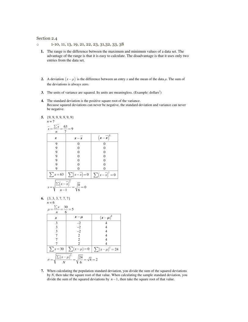
2.4 EXERCISE SOLUTIONS 1. The range is the difference between the maximum and minimum values of a data set. The
advantage of the range is that it is easy to calculate. The disadvantage is that it uses only two entries from the data set.
58 CHAPTER 2 Ň DESCRIPTIVE STATISTICS
Copyright © 2012 Pearson Education, Inc. Publishing as Prentice Hall.
2. A deviation x N� is the difference between an entry x and the mean of the data µ. The sum of the deviations is always zero.
3. The units of variance are squared. Its units are meaningless. (Example: dollars2) 4. The standard deviation is the positive square root of the variance. Because squared deviations can never be negative, the standard deviation and variance can never
be negative. 5. {9, 9, 9, 9, 9, 9, 9} n = 7
63
97
xx
n�
� � �
x �x x �2
x x
9 0 0 9 0 0 9 0 0 9 0 0 9 0 0 9 0 0 9 0 0
63x �� 0x x� �� 20x x� ��
2
00
1 6
x xs
n
� �� � �
�
6. {3, 3, 3, 7, 7, 7} n = 6
30
56
xn
N�
� � �
x �x N � 2x N 3 –2 4 3 –2 4 3 –2 4 7 2 4 7 2 4 7 2 4
30x �� 0x N� �� 224x N� ��
2
244 2
6
x
N
NT
� �� � � �
7. When calculating the population standard deviation, you divide the sum of the squared deviations
by N, then take the square root of that value. When calculating the sample standard deviation, you divide the sum of the squared deviations by 1n� , then take the square root of that value.
CHAPTER 2 Ň DESCRIPTIVE STATISTICS 59
Copyright © 2012 Pearson Education, Inc. Publishing as Prentice Hall.
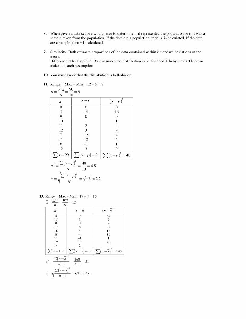
8. When given a data set one would have to determine if it represented the population or if it was a sample taken from the population. If the data are a population, then T is calculated. If the data are a sample, then s is calculated.
9. Similarity: Both estimate proportions of the data contained within k standard deviations of the
mean. Difference: The Empirical Rule assumes the distribution is bell-shaped. Chebychev’s Theorem
makes no such assumption. 10. You must know that the distribution is bell-shaped. 11. Range = Max – Min = 12 – 5 = 7
90
910
xN
N�
� � �
x �x N � 2x N 9 0 0 5 –4 16 9 0 0
10 1 1 11 2 4 12 3 9 7 –2 4 7 –2 4 8 –1 1
12 3 9 90x �� 0x N� �� 2
48x N� ��
2
2 484.8
10
x
N
NT
� �� � �
2
4.8 2.2x
N
NT
� �� � x
60 CHAPTER 2 Ň DESCRIPTIVE STATISTICS
Copyright © 2012 Pearson Education, Inc. Publishing as Prentice Hall.
12. Range = Max – Min = 25 – 15 = 10
266
1914
xN
N�
� � �
x �x N � 2x N 18 –1 1 20 1 1 19 0 0 21 2 4 19 0 0 17 –2 4 15 –4 16 17 –2 4 25 6 36 22 3 9 19 0 0 20 1 1 16 –3 9 18 –1 1
90x �� 0x N� �� 286x N� ��
2
2 866.1
14
x
N
NT
� �� � x
2
862.5
14
x
N
NT
� �� � x
13. Range = Max – Min = 19 – 4 = 15
108
129
xx
n�
� � �
x �x x �2
x x
4 –8 64 15 3 9 9 –3 9
12 0 0 16 4 16 8 –4 16
11 –1 1 19 7 49 14 2 4
108x�� 0x x� �� 2168x x� ��
2
2 16821
1 9 1
x xs
n
� �� � �
� �
2
21 4.61
x xs
n
� �� � x
�
CHAPTER 2 Ň DESCRIPTIVE STATISTICS 61
Copyright © 2012 Pearson Education, Inc. Publishing as Prentice Hall.
14. Range = Max – Min = 28 – 7 = 21
238
18.313
xx
n�
� � x
x �x x �2
x x
28 9.7 94.09 25 6.7 44.89 21 2.7 7.29 15 –3.3 10.89 7 –11.3 127.69 14 –4.3 18.49 9 –9.3 86.49 27 8.7 75.69 21 2.7 7.29 24 5.7 32.49 14 –4.3 18.49 17 –1.3 1.69 16 –2.3 5.29
238x �� 0x x� x� 2530.77x x� ��
2
2 530.7744.2
1 13 1
x xs
n
� �� � x
� �
2
530.776.7
1 12
x xs
n
� �� � x
�
15. Range = Max – Min = 96 – 23 = 73 16. Range = Max – Min = 34 – 24 = 10 17. Range = Max – Min = 98 – 74 = 24 18. Range = Max – Min = 6.7 – 0.5 = 6.2 19a. Range = Max – Min = 38.5 – 20.7 = 17.8 b. Range = Max – Min = 60.5 – 20.7 = 39.8 20. Changing the maximum value of the data set greatly affects the range. 21. Graph (a) has a standard deviation of 24 and graph (b) has a standard deviation of 16 because
graph (a) has more variability. 22. Graph (a) has a standard deviation of 2.4 and graph (b) has a standard deviation of 5 because
graph (b) has more variability. 23. Company B. An offer of $33,000 is two standard deviations from the mean of Company A’s
starting salaries, which makes it unlikely. The same offer is within one standard deviation of the mean of Company B’s starting salaries, which makes the offer likely.
CHAPTER 2 Ň DESCRIPTIVE STATISTICS 67
Copyright © 2012 Pearson Education, Inc. Publishing as Prentice Hall.
2
0.004676890.02418
1 8
x xs
n
� �� � x
�
b. It appears form the data that the batting averages for Team A are more variable than the batting averages for Team B. The batting averages for Team A have a higher mean and a higher median than those for Team B.
29a. Greatest sample standard deviation: (ii) Data set (ii) has more entries that are farther away from the mean. Least sample standard deviation: (iii) Data set (iii) has more entries that are close to the mean. b. The three data sets have the same mean but have different standard deviations. 30a. Greatest sample standard deviation: (i) Data set (i) has more entries that are farther away from the mean. Least sample standard deviation: (iii) Data set (iii) has more entries that are close to the mean. b. The three data sets have the same mean, median, and mode, but have different standard
deviations. 31a. Greatest sample standard deviation: (ii) Data set (ii) has more entries that are farther away from the mean. Least sample standard deviation: (iii) Data set (iii) has more entries that are close to the mean. b. The three data sets have the same mean, median, and mode, but have different standard
deviations. 32a. Greatest sample standard deviation: (iii) Data set (iii) has more entries that are farther away from the mean. Least sample standard deviation: (i) Data set (i) has more entries that are close to the mean. b. The three data sets have the same mean and median but have different modes and standard
deviations.
33. 1300, 1700 1500 1 200 , 1500 1 200 , x s x sl � � l � �
68% of the farms have values between $1300 and $1700 per acre. 34. 95% of the data falls between 2x s� and 2x s� . 2 2400 2 450 1500x s� � � �
2 2400 2 450 3300x s� � � � 95% of the farms have values between $1500 and $3300 per acre. 35a. 75n � 68%(75) = (0.68)(75) 51 farms have values between $1300 and $1700 per acre. b. 25n � 68%(25) = (0.68)(25) 17 farms have values between $1300 and $1700 per acre.
68 CHAPTER 2 Ň DESCRIPTIVE STATISTICS
Copyright © 2012 Pearson Education, Inc. Publishing as Prentice Hall.
36a. 40n � 95%(40) = (0.95)(40) 38 farms have values between $1500 and $3300 per acre. b. 20n � 95%(20) = (0.95)(20) 19 farms have values between $1500 and $3300 per acre. 37. 1500x� 200s � {$950, $1000, $2000, $2180} are outliers. They are more than 2 standard deviations from the
mean (1100, 1900). $2180 is very unusual because it is more than 3 standard deviations from the mean.
38. 2400x� 450s � {$1045, $1490, $3325, $3800} are outliers. They are more than 2 standard deviations from the
mean (1500, 3300). $1045 and $3800 are very unusual because they are more than 3 standard deviations from the mean.
39. 2 , 2 1.14, 5.5x s x s� � l are 2 standard deviations from the mean.
22
1 1 11 1 1 0.75
42k� � � � � � ºAt least 75% of the eruption times lie between 1.14 and 5.5
minutes. If n = 32, at least (0.75)(32) = 24 eruptions will lie between 1.14 and 5.5 minutes.
40. 22
1 1 11 1 1 0.75
42k� � � � � �
At least 75% of the 400-meter dash times lie within 2 standard deviations of the mean.
2 , 2 54.97, 59.17x s x s� � l
At least 75% of the 400-meter dash times lie between 54.97 and 59.17 seconds. 41.
x f xf �x x �
2x x �
2x x f
0 5 0 –2.1 4.41 22.05 1 11 11 –1.1 1.21 13.31 2 7 14 –0.1 0.01 0.07 3 10 30 0.9 0.81 8.10 4 7 28 1.9 3.61 25.27
n = 40 83xf �� 268.8x x f� ��
83
2.140
xfx
n�
� � x
2
68.81.3
1 39
x x fs
n
� �� � x
�
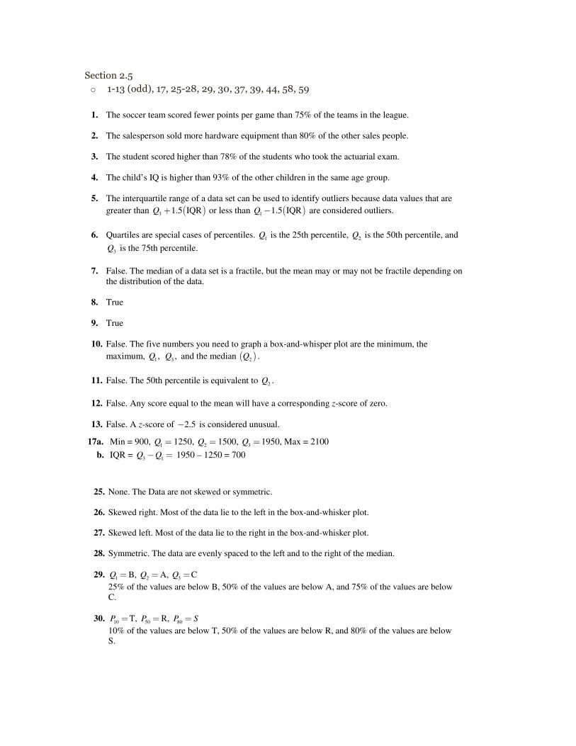
Section 2.5 o 1-13 (odd), 17, 25-28, 29, 30, 37, 39, 44, 58, 59
78 CHAPTER 2 Ň DESCRIPTIVE STATISTICS
Copyright © 2012 Pearson Education, Inc. Publishing as Prentice Hall.
7a. Best actor: 43.7, 8.7N T� � Best actress: 35.9, 11.4N T� �
b. Sean Penn: 48 43.7
48: 0.498.7
xx z
NT� �
� � � x
Kate Winslet: 33 35.9
33: 0.2511.4
xx z
NT� �
� � � x�
c. Sean Penn’s age is 0.49 standard deviation above the mean of the best actors. Kate Winslet’s age is 0.25� standard deviation below the mean of the best actresses. Neither actor’s age is unusual.
2.5 EXERCISE SOLUTIONS 1. The soccer team scored fewer points per game than 75% of the teams in the league. 2. The salesperson sold more hardware equipment than 80% of the other sales people. 3. The student scored higher than 78% of the students who took the actuarial exam. 4. The child’s IQ is higher than 93% of the other children in the same age group. 5. The interquartile range of a data set can be used to identify outliers because data values that are
greater than 3 1.5 IQRQ � or less than 1 1.5 IQRQ � are considered outliers. 6. Quartiles are special cases of percentiles. 1Q is the 25th percentile, 2Q is the 50th percentile, and
3Q is the 75th percentile. 7. False. The median of a data set is a fractile, but the mean may or may not be fractile depending on
the distribution of the data. 8. True 9. True 10. False. The five numbers you need to graph a box-and-whisper plot are the minimum, the
maximum, 1,Q 3 ,Q and the median 2Q . 11. False. The 50th percentile is equivalent to 2Q . 12. False. Any score equal to the mean will have a corresponding z-score of zero. 13. False. A z-score of 2.5� is considered unusual. 14. True 15a. Min = 10, 1Q � 13, 2Q � 15, 3Q �17, Max = 20 b. IQR = 3 1Q Q� � 17 – 13 = 4 16a. Min = 100, 1Q � 130, 2Q � 205, 3Q �270, Max = 320
CHAPTER 2 Ň DESCRIPTIVE STATISTICS 79
Copyright © 2012 Pearson Education, Inc. Publishing as Prentice Hall.
b. IQR = 3 1Q Q� � 270 – 130 = 140 17a. Min = 900, 1Q � 1250, 2Q � 1500, 3Q �1950, Max = 2100 b. IQR = 3 1Q Q� � 1950 – 1250 = 700 18a. Min = 25, 1Q � 50, 2Q � 65, 3Q �70, Max = 85 b. IQR = 3 1Q Q� � 70 – 50 = 20 19a. Min = 1.9� , 1Q � 0.5� , 2Q � 0.1, 3Q �0.7, Max = 2.1
b. IQR = 3 1Q Q� � 0.7 0.5� � = 1.2 20a. Min = 1.3� , 1Q � 0.3� , 2Q � 0.2, 3Q �0.4, Max = 2.1
b. IQR = 3 1Q Q� � 0.4 0.3� � = 0.7 21a.
Min = 24, 1Q � 28, 2Q � 35, 3Q �41, Max = 60 b.
22a.
Min = 150, 1Q � 172, 2Q � 177, 3Q �180, Max = 182 b.
23a.
Min = 1, 1Q � 4.5, 2Q � 6, 3Q �7.5, Max = 9
80 CHAPTER 2 Ň DESCRIPTIVE STATISTICS
Copyright © 2012 Pearson Education, Inc. Publishing as Prentice Hall.
b.
24a.
Min = 1, 1Q � 3, 2Q � 5, 3Q �8, Max = 9 b.
25. None. The Data are not skewed or symmetric. 26. Skewed right. Most of the data lie to the left in the box-and-whisker plot. 27. Skewed left. Most of the data lie to the right in the box-and-whisker plot. 28. Symmetric. The data are evenly spaced to the left and to the right of the median. 29. 1Q � B, 2Q � A, 3Q �C 25% of the values are below B, 50% of the values are below A, and 75% of the values are below
C. 30. 10P �T, 50P � R, 80P S� 10% of the values are below T, 50% of the values are below R, and 80% of the values are below
S. 31a. 1Q � 2, 2Q � 4, 3Q �5 b.
32a. 1Q � 2, 2Q � 4.5, 3Q �6.5
CHAPTER 2 Ň DESCRIPTIVE STATISTICS 81
Copyright © 2012 Pearson Education, Inc. Publishing as Prentice Hall.
b.
33a. 1Q � 3, 2Q � 3.85, 3Q �5.2 b.
34a. 1Q � 15.125, 2Q � 15.8, 3Q �17.65 b.
35a. 5 b. 50% c. 25% 36a. $17.65 b. 50% c. 50% 37. A 1.43zº �� B 0zº � C 2.14zº � The z-score 2.14 is unusual because it is so large. 38. A 1.54zº �� B 0.77zº � C 1.54zº � None of the z-scores are unusual.
39a. Statistics: 75 63
75 1.717
xx z
NT� �
� º � � x
Biology: 25 23
25 0.513.9
xx z
NT� �
� º � � x
b. The student had a better score on the statistics test.
82 CHAPTER 2 Ň DESCRIPTIVE STATISTICS
Copyright © 2012 Pearson Education, Inc. Publishing as Prentice Hall.
40a. Statistics: 60 63
60 0.437
xx z
NT� �
� º � � x�
Biology: 22 23
22 0.263.9
xx z
NT� �
� º � � x�
b. The student had a better score on the biology test.
41a. Statistics: 78 63
78 2.147
xx z
NT� �
� º � � x
Biology: 29 23
29 1.543.9
xx z
NT� �
� º � � x
b. The student had a better score on the statistics test.
42a. Statistics: 63 63
63 07
xx z
NT� �
� º � � �
Biology: 23 23
23 03.9
xx z
NT� �
� º � � �
b. The student performed equally well on the two tests.
43a. 34,000 35,000
34,000 0.442,250
xx z
NT� �
� º � � x�
37,000 35,000
37,000 0.892,250
xx z
NT� �
� º � � x
30,000 35,000
30,000 2.222,250
xx z
NT� �
� º � � x�
The tire with a life span of 30,000 miles has an unusually short life span.
b. 30,500 35,000
30,500 22,250
xx z
NT� �
� º � � �� º 2.5th percentile
37,250 35,000
37,250 12,250
xx z
NT� �
� º � � � º84th percentile
35,000 35,000
35,000 02,250
xx z
NT� �
� º � � � º 50th percentile
44a. 34 33
34 0.254
xx z
NT� �
� º � � �
30 33
30 0.754
xx z
NT� �
� º � � ��
42 33
42 2.254
xx z
NT� �
� º � � �
The fruit fly with a life span of 42 days has an unusually long life span.
b. 29 33
29 14
xx z
NT� �
� º � � �� º 16th percentile
41 33
41 24
xx z
NT� �
� º � � � º 97.5th percentile
25 33
25 24
xx z
NT� �
� º � � �� º 2.5th percentile
CHAPTER 2 Ň DESCRIPTIVE STATISTICS 85
Copyright © 2012 Pearson Education, Inc. Publishing as Prentice Hall.
58. PercentileNumber of data values less than
100Total number of data values
3100 4th percentile
73
x� ¸
� ¸ x
59. PercentileNumber of data values less than
100Total number of data values
30100 41st percentile
73
x� ¸
� ¸ x
60a.
1Q � 9, 2Q � 11, 3Q �13 IQR 3 1 13 9 4Q Q� � � � � 1.5 IQR 6q �
1
3
1.5 IQR 9 6 3
1.5 IQR 13 6 19
Q
Q
� q � � �
� q � � �
Any values less than 6 or greater than 19 is an outlier. So, 2 and 24 are outliers. b.
61a.
1Q � 73, 2Q � 75, 3Q �79 IQR 3 1 79 73 6Q Q� � � � � 1.5 IQR 9q �
1
3
1.5 IQR 73 9 64
1.5 IQR 79 9 88
Q
Q
� q � � �
� q � � �
Any values less than 64 or greater than 88 is an outlier. So, 62 and 95 are outliers. b.


![[PPT]Codes and Conventions of Film Musicals - North …facweb.northseattle.edu/jclapp/HUM 110/Handouts and... · Web viewCodes and Conventions of Film Musicals Introduction to American](https://img.pdfslide.us/doc/110x75/5acee6627f8b9a8b1e8c0b47/pptcodes-and-conventions-of-film-musicals-north-110handouts-andweb-viewcodes.jpg)