Embed Size (px)
Citation preview
Report
Palmerston North Area Traffic Model - Model Development and Validation Report Prepared for By Beca Ltd (Beca) 77-330-577
23 December 2014
© Beca 2014 (unless Beca has expressly agreed otherwise with the Client in writing).
This report has been prepared by Beca on the specific instructions of our Client. It is solely for our Client’s use for the purpose for which it is intended in accordance with the agreed scope of work. Any use or reliance by any person contrary to the above, to which Beca has not given its prior written consent, is at that person's own risk.
Palmerston North Area Traffic Model - Model Development and Validation Report
Beca // 23 December 2014 3818357 // NZ1-9382215-56 0.56
Revision History
Revision Nº Prepared By Description Date
A Nyan Aung Lin A draft for client and peer reviewer 15/08/2014
B Nyan Aung Lin Revised with peer review’s comments
19/11/2014
C Nyan Aung Lin Revised in response to Peer Review Report
23/12/2014
Document Acceptance
Action Name Signed Date
Prepared by Nyan Aung Lin
Reviewed by Alan Kerr
Approved by Andrew Murray
on behalf of Beca Ltd
Palmerston North Area Traffic Model - Model Development and Validation Report
Beca // 23 December 2014 // Page 1 3818357 // NZ1-9382215-56 0.56
Table of Contents 1 Introduction .......................................................................................................... 4
1.1 Purpose ........................................................................................................................ 4 1.2 General Model Purpose and Type ............................................................................... 4 1.3 Functionality ................................................................................................................. 4 1.4 Guiding Principles ........................................................................................................ 4 1.5 Report Structure ........................................................................................................... 5
2 Data Sources and Requirements ......................................................................... 6 2.1 Land Use/Demographic Data ....................................................................................... 6 2.2 Origin/Destination Travel Data ..................................................................................... 6 2.3 Network Data ............................................................................................................... 6 2.4 Traffic Flow Data .......................................................................................................... 6 2.5 Journey Time Data ....................................................................................................... 9
3 Base Model Specification .................................................................................. 10 3.1 Model Structure .......................................................................................................... 10 3.2 Model Extent .............................................................................................................. 11 3.3 Zone System .............................................................................................................. 12 3.4 Network Representation ............................................................................................ 13 3.5 Base Year and Time Periods ..................................................................................... 16 3.6 Expansion factors ....................................................................................................... 19 3.7 Trip Purposes ............................................................................................................. 19 3.8 Household Structure Model ....................................................................................... 20
4 Trip Generation Model ........................................................................................ 22 4.1 Base Year Land Use Data ......................................................................................... 22 4.2 Trip Production/Attraction Models .............................................................................. 22 4.3 External Models ......................................................................................................... 26 4.4 Airport Model .............................................................................................................. 26
5 Trip Distribution Model ....................................................................................... 27 5.1 Model Form ................................................................................................................ 27 5.2 Impedance Function................................................................................................... 27 5.3 Generalised Cost ....................................................................................................... 27 5.4 Time, Distance and Toll Skims .................................................................................. 28 5.5 Demand/Supply Convergence ................................................................................... 29 5.6 Calibration of HBW Distribution Model....................................................................... 29 5.7 Sector to Sector K Factor ........................................................................................... 34 5.8 Adopted Distribution Parameters ............................................................................... 35
6 Time Period Model .............................................................................................. 37 6.1 Model Form ................................................................................................................ 37 6.2 Period and Direction Factors ..................................................................................... 37
Palmerston North Area Traffic Model - Model Development and Validation Report
Beca // 23 December 2014 // Page 2 3818357 // NZ1-9382215-56 0.56
6.3 Peak Hour Demands .................................................................................................. 39
7 Assignment Model .............................................................................................. 40 7.1 Model Form ................................................................................................................ 40 7.2 Generalised Cost for Path Building ............................................................................ 40
8 Model Calibration and Validation Methodology ................................................ 42 8.1 Calibration Approach.................................................................................................. 42 8.2 Key Validation Checks ............................................................................................... 42
9 Matrix Estimation Process ................................................................................. 43 9.1 Light Vehicle Matrix Adjustment ................................................................................. 43 9.2 Commercial Vehicle Matrix Development .................................................................. 51
10 Model Validation Results.................................................................................... 53 10.1 Statistical Tests .......................................................................................................... 53 10.2 Flow Validation ........................................................................................................... 55 10.3 Turning Flow Validation ............................................................................................. 60 10.4 Travel Time Validation ............................................................................................... 63 10.5 Heavy Vehicle Validation ........................................................................................... 69 10.6 Convergence .............................................................................................................. 72
11 Conclusions ........................................................................................................ 72
Palmerston North Area Traffic Model - Model Development and Validation Report
Beca // 23 December 2014 // Page 3 3818357 // NZ1-9382215-56 0.56
Executive Summary
This document sets out the work undertaken to develop a traffic model of Palmerston North city and the surrounding area (the Palmerston North Area Traffic Model, PNATM). This is the second significant deliverable for this project, the first being the model scoping report, delivered in January 2014. This report only relates to the base year model development and validation process. The future year model development and forecasting process will be documented in a separate report.
A previous model had been developed for Palmerston North using the T model software. This model was used as a basis for the development of PNATM. A significant amount of data collection and analysis was also undertaken by Palmerston North City Council (PNCC) and Beca. New cost effective data collection techniques were adopted, including using commercial GPS data and Bluetooth vehicle tracking.
A three stage traffic model has been developed using the CUBE VOYAGER software. The model consists of 212 zones, and a series of links and nodes (representing road links and intersections respectively). The model reflects a base year of 2013 and covers AM, PM and interpeak periods.
Demand matrices have been produced for light and heavy vehicles using a combination of observed data and synthetic matrix development. These have been calibrated using count and turn data.
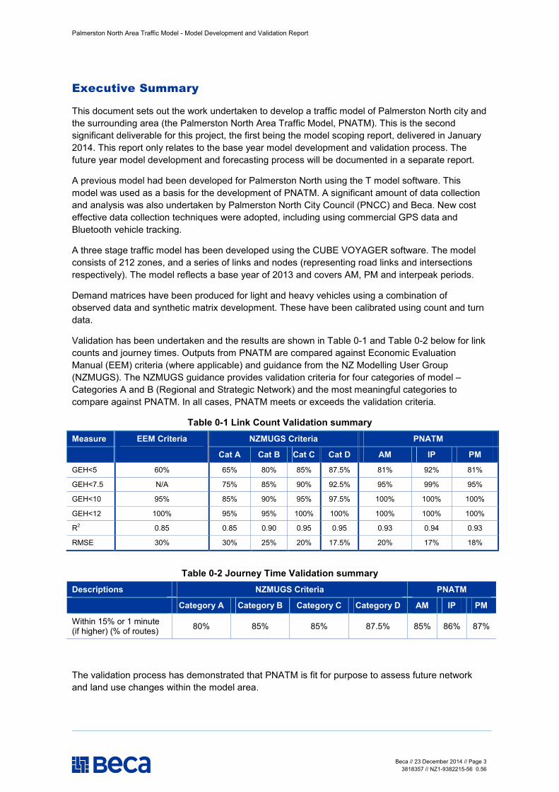
Validation has been undertaken and the results are shown in Table 0-1 and Table 0-2 below for link counts and journey times. Outputs from PNATM are compared against Economic Evaluation Manual (EEM) criteria (where applicable) and guidance from the NZ Modelling User Group (NZMUGS). The NZMUGS guidance provides validation criteria for four categories of model – Categories A and B (Regional and Strategic Network) and the most meaningful categories to compare against PNATM. In all cases, PNATM meets or exceeds the validation criteria.
Table 0-1 Link Count Validation summary Measure EEM Criteria NZMUGS Criteria PNATM
Cat A Cat B Cat C Cat D AM IP PM
GEH<5 60% 65% 80% 85% 87.5% 81% 92% 81%
GEH<7.5 N/A 75% 85% 90% 92.5% 95% 99% 95%
GEH<10 95% 85% 90% 95% 97.5% 100% 100% 100%
GEH<12 100% 95% 95% 100% 100% 100% 100% 100%
R2 0.85 0.85 0.90 0.95 0.95 0.93 0.94 0.93
RMSE 30% 30% 25% 20% 17.5% 20% 17% 18%
Table 0-2 Journey Time Validation summary
Descriptions NZMUGS Criteria PNATM
Category A Category B Category C Category D AM IP PM
Within 15% or 1 minute (if higher) (% of routes) 80% 85% 85% 87.5% 85% 86% 87%
The validation process has demonstrated that PNATM is fit for purpose to assess future network and land use changes within the model area.

Palmerston North Area Traffic Model - Model Development and Validation Report
Beca // 23 December 2014 // Page 4 3818357 // NZ1-9382215-56 0.56
1 Introduction
1.1 Purpose
This report outlines the structure, specification and validation for the Palmerston North Area Traffic Model (PNATM). The PNATM has been developed to provide traffic predictions for the Palmerston North City for use in local and regional transport planning.
The model was developed in accordance with the scoping report, “Palmerston North Area Traffic Model – Model Scoping and Specification, Beca, January2014”, which was issued to PNCC and the Peer Reviewer, Tim Kelly. The scoping report also describes the previous version of the model “T Model” and discusses its functionalities and limitations.
1.2 General Model Purpose and Type
Based on the RFT and subsequent discussions with PNCC staff, we have assessed the broad purpose of the model to be to provide predictions of current and future traffic flows and network performance in the study area. Although intended for general transport planning purposes, it is expected that the model would form the basis for development of models for more detailed analysis of specific projects.
1.3 Functionality
We have assessed the key functional requirements of the model as follows:
n Provide a reliable replication of existing traffic patterns and network performance, suitable to the purpose of the model;
n Relate traffic flows directly to input land use data; n Provide predictions of changes in traffic flows and patterns in future years, in response to
changes in land use or the network; n Provide strong analysis and graphical output capabilities along with a good GIS interface (for
both inputs and outputs); and n Provide a basis for more detailed models of specific projects.
1.4 Guiding Principles
The model has been developed with consideration of some key guiding principles, including:
n Seek to be transparent and usable by other modellers (as much as is feasible for such models); n Use common software and techniques where feasible; n Be based on common NZ modelling practice; n Keep it simple. This means a focus on the key functional requirements without overly complex
model functionality, especially in areas not critical to this context; and n Recognise that some judgement call will be required in the model design, but that these should
be based on appropriate reasons and decided in consultation with the peer reviewer.

Palmerston North Area Traffic Model - Model Development and Validation Report
Beca // 23 December 2014 // Page 5 3818357 // NZ1-9382215-56 0.56
1.5 Report Structure
The remainder of this report is structured as follows:
Chapter 2 Describes the data available for the model development
Chapter 3 Details the general specification and structure of the model
Chapter 4 Describes the Trip Generation Model
Chapter 5 Describes the Trip Distribution Model
Chapter 6 Describes the Time Period Model
Chapter 7 Describes the Assignment Model
Chapter 8 Describes the Calibration/Validation Methodology
Chapter 9 Describes the matrix adjustment process
Chapter 10 Describes the model validation results
Chapter 11 Describes the summary and conclusions of this report

Palmerston North Area Traffic Model - Model Development and Validation Report
Beca // 23 December 2014 // Page 6 3818357 // NZ1-9382215-56 0.56
2 Data Sources and Requirements
This chapter outlines the data requirements, the available data and identifies requirements for new data collected as part of this study.
2.1 Land Use/Demographic Data
The most up to date census data was collected in 2013 and has represented a key input to the model. The census data used includes population, household and employment data. ,. School roll data is available and has been sourced from the ‘schools directory’ on the Ministry of Education website, however the tertiary directory does not include roll information. This was sourced directly from PNCC and Massey University.
2.2 Origin/Destination Travel Data
The key source of origin-destination data was the census Journey to work (JTW) data. Statistics New Zealand typically supplies this at census area unit (CAU) level. In order to inform the model, this was further disaggregated to meshblock level from the population and employment data, then aggregated to traffic zones. Although a very good source of travel data, this only applies to the commuter trip.
The electronic road user charges (ERUC) data (as implemented in TeamView Clarity) has been used to estimate truck matrices. Although some light (diesel) vehicles are captured in this data, it is predominantly sourced from trucks (approximately 40% of heavy vehicle RUC is captured through the ERUC system).
Project specific origin-destination surveys were not undertaken for this study. The model generates ‘synthetic’ matrices from trip generation and distribution modules so it does not need the survey data to build the matrices.
The synthetic model, however, does not generate external-to-external (‘through’) traffic as that is not a function of internal land use. The old traffic model includes a through-traffic matrix, derived from origin-destination surveys in the late 1990’s. GPS-derived data from TeamView Clarity has been used to estimate through truck movements, and specific Bluetooth device has been used to collect information on key external to external trips. A separate report has been produced on the Bluetooth approach and the results as used in the model.
2.3 Network Data
The model networks have been developed from a range of sources, including the previous model, GIS road centreline data, SCATS signal phasing data, site visits and aerial photos.
2.4 Traffic Flow Data
PNCC have an extensive data set of traffic counts, which have been the main source of traffic data for this model build. These have been augmented by similar data from NZTA and the Manawatu District Council.
We have identified six sets of traffic counts as follows:
n Counts from PNCC’s standard count program n Special PNCC counts done to coincide with 2013 census period n PNCC ‘special’ counts on low-volume roads
Palmerston North Area Traffic Model - Model Development and Validation Report
Beca // 23 December 2014 // Page 7 3818357 // NZ1-9382215-56 0.56
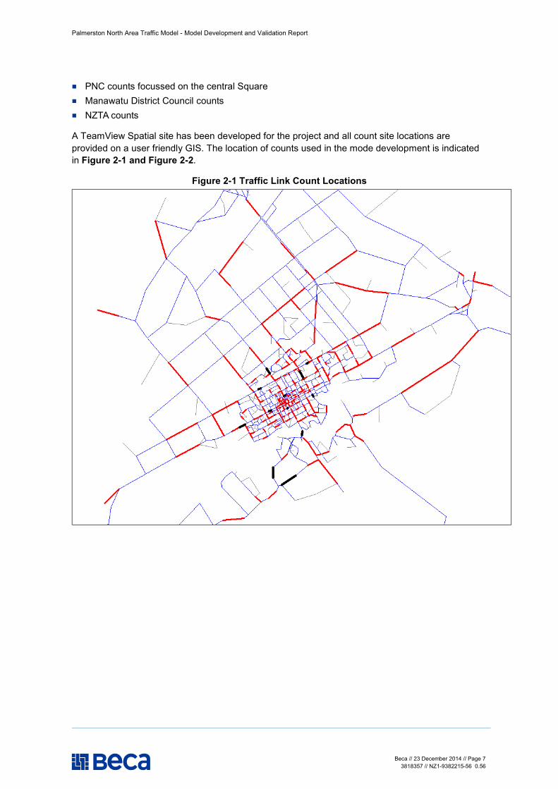
n PNC counts focussed on the central Square n Manawatu District Council counts n NZTA counts
A TeamView Spatial site has been developed for the project and all count site locations are provided on a user friendly GIS. The location of counts used in the mode development is indicated in Figure 2-1 and Figure 2-2.
Figure 2-1 Traffic Link Count Locations
Palmerston North Area Traffic Model - Model Development and Validation Report
Beca // 23 December 2014 // Page 8 3818357 // NZ1-9382215-56 0.56
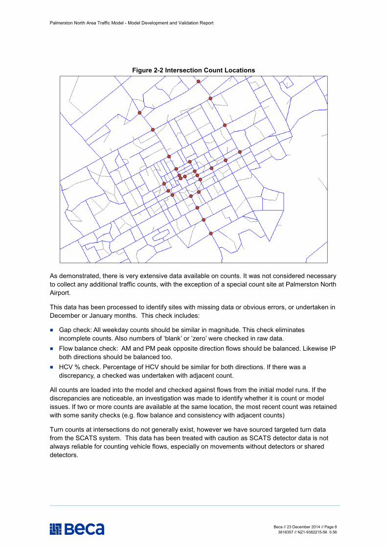
Figure 2-2 Intersection Count Locations
As demonstrated, there is very extensive data available on counts. It was not considered necessary to collect any additional traffic counts, with the exception of a special count site at Palmerston North Airport.
This data has been processed to identify sites with missing data or obvious errors, or undertaken in December or January months. This check includes:
n Gap check: All weekday counts should be similar in magnitude. This check eliminates incomplete counts. Also numbers of ‘blank’ or ’zero’ were checked in raw data.
n Flow balance check: AM and PM peak opposite direction flows should be balanced. Likewise IP both directions should be balanced too.
n HCV % check. Percentage of HCV should be similar for both directions. If there was a discrepancy, a checked was undertaken with adjacent count.
All counts are loaded into the model and checked against flows from the initial model runs. If the discrepancies are noticeable, an investigation was made to identify whether it is count or model issues. If two or more counts are available at the same location, the most recent count was retained with some sanity checks (e.g. flow balance and consistency with adjacent counts)
Turn counts at intersections do not generally exist, however we have sourced targeted turn data from the SCATS system. This data has been treated with caution as SCATS detector data is not always reliable for counting vehicle flows, especially on movements without detectors or shared detectors.
Palmerston North Area Traffic Model - Model Development and Validation Report
Beca // 23 December 2014 // Page 9 3818357 // NZ1-9382215-56 0.56
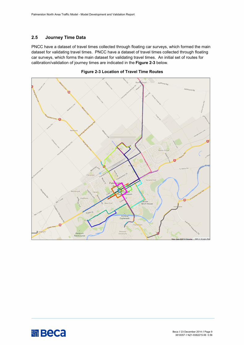
2.5 Journey Time Data
PNCC have a dataset of travel times collected through floating car surveys, which formed the main dataset for validating travel times. PNCC have a dataset of travel times collected through floating car surveys, which forms the main dataset for validating travel times. An initial set of routes for calibration/validation of journey times are indicated in the Figure 2-3 below.
Figure 2-3 Location of Travel Time Routes
Palmerston North Area Traffic Model - Model Development and Validation Report
Beca // 23 December 2014 // Page 10 3818357 // NZ1-9382215-56 0.56
3 Base Model Specification
This chapter describes the general model structure and specifies its key components.
3.1 Model Structure
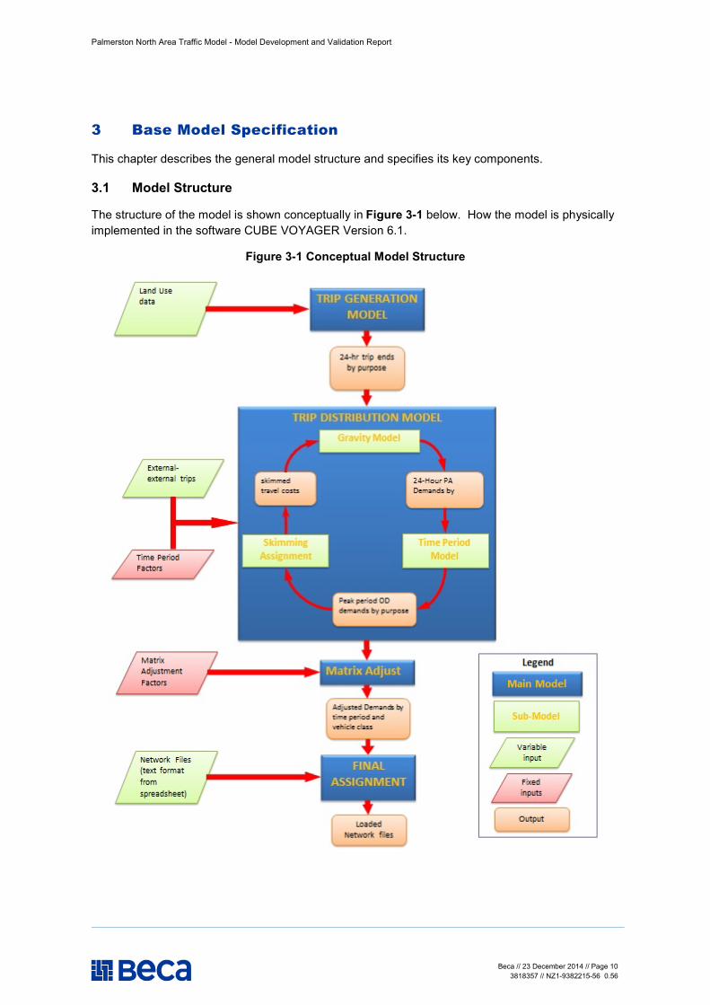
The structure of the model is shown conceptually in Figure 3-1 below. How the model is physically implemented in the software CUBE VOYAGER Version 6.1.
Figure 3-1 Conceptual Model Structure
Palmerston North Area Traffic Model - Model Development and Validation Report
Beca // 23 December 2014 // Page 11 3818357 // NZ1-9382215-56 0.56
3.2 Model Extent
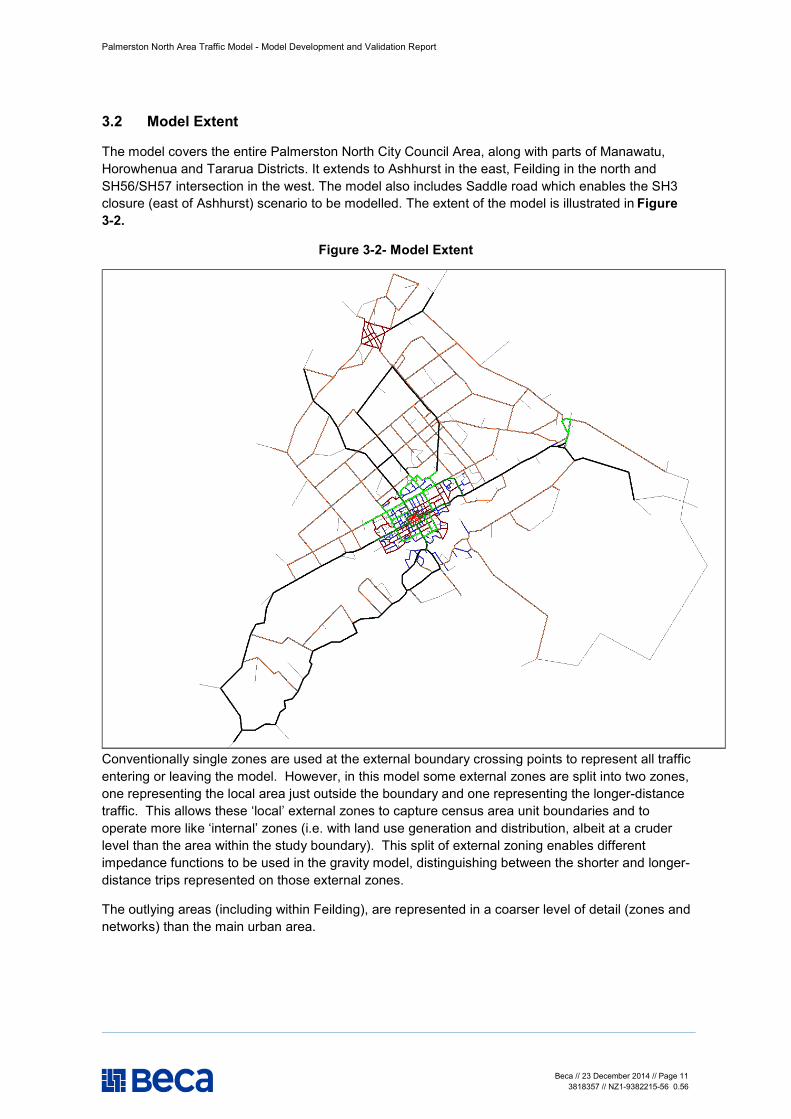
The model covers the entire Palmerston North City Council Area, along with parts of Manawatu, Horowhenua and Tararua Districts. It extends to Ashhurst in the east, Feilding in the north and SH56/SH57 intersection in the west. The model also includes Saddle road which enables the SH3 closure (east of Ashhurst) scenario to be modelled. The extent of the model is illustrated in Figure 3-2.
Figure 3-2- Model Extent
Conventionally single zones are used at the external boundary crossing points to represent all traffic entering or leaving the model. However, in this model some external zones are split into two zones, one representing the local area just outside the boundary and one representing the longer-distance traffic. This allows these ‘local’ external zones to capture census area unit boundaries and to operate more like ‘internal’ zones (i.e. with land use generation and distribution, albeit at a cruder level than the area within the study boundary). This split of external zoning enables different impedance functions to be used in the gravity model, distinguishing between the shorter and longer-distance trips represented on those external zones.
The outlying areas (including within Feilding), are represented in a coarser level of detail (zones and networks) than the main urban area.
Palmerston North Area Traffic Model - Model Development and Validation Report
Beca // 23 December 2014 // Page 12 3818357 // NZ1-9382215-56 0.56
3.3 Zone System
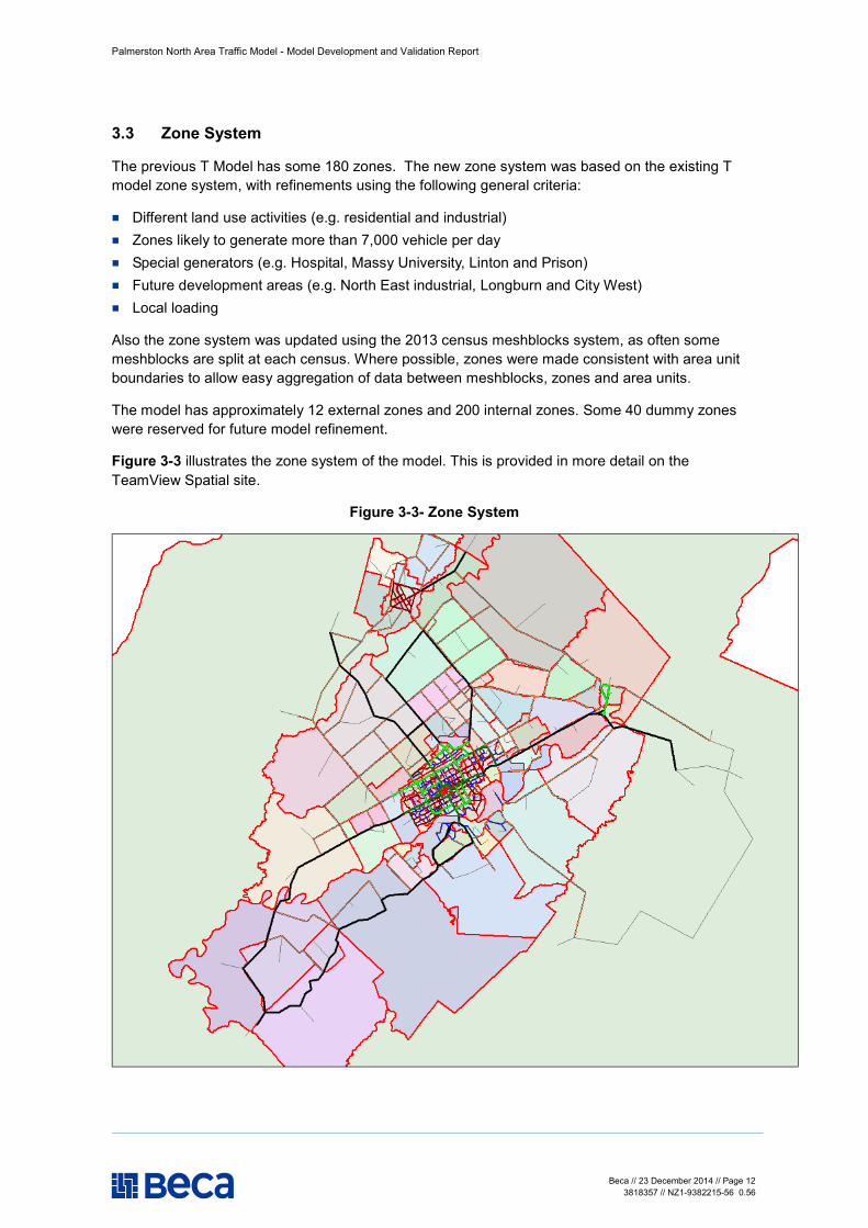
The previous T Model has some 180 zones. The new zone system was based on the existing T model zone system, with refinements using the following general criteria:
n Different land use activities (e.g. residential and industrial) n Zones likely to generate more than 7,000 vehicle per day n Special generators (e.g. Hospital, Massy University, Linton and Prison) n Future development areas (e.g. North East industrial, Longburn and City West) n Local loading
Also the zone system was updated using the 2013 census meshblocks system, as often some meshblocks are split at each census. Where possible, zones were made consistent with area unit boundaries to allow easy aggregation of data between meshblocks, zones and area units.
The model has approximately 12 external zones and 200 internal zones. Some 40 dummy zones were reserved for future model refinement.
Figure 3-3 illustrates the zone system of the model. This is provided in more detail on the TeamView Spatial site.
Figure 3-3- Zone System
Palmerston North Area Traffic Model - Model Development and Validation Report
Beca // 23 December 2014 // Page 13 3818357 // NZ1-9382215-56 0.56
3.4 Network Representation
The model represents network performance via speed-flow curves applied on links and with explicit, turn-level modelling of intersection delays.
3.4.1 Flow and Capacity Units
The model operates using flow units of vehicles rather than passenger-car units (pcus). The link capacities were coded in vehicles per hour.
3.4.2 Link Types and Parameters
In order to provide consistent coding of similar sections of road, a link-type classification system was developed. All links were classified in terms of their road environment and given a relevant link type code. These link type classifications were used to allocate the parameters of the speed flow curves (e.g. free speed and capacity) and any relevant routing parameters (e.g. site specific weightings to reflect influences on route choice other than time and distance, such as signage, comfort etc).
The speed-flow functions require a ‘free-speed’ (typical speed with no other vehicles interrupting travel) rather than a speed limit. The free speeds were coded based on the speed limit, generally slightly higher for higher-standard roads and slightly lower for access or residential-type roads. Those relationships were adjusted during the model calibration process but a consistent approach using the link type classification was used rather than only adjusting the sample of roads for which travel time data is available.
3.4.3 Speed-Flow Curves
The speed-flow curves are based on the Akcelik speed-flow functions, as used in the Auckland, Christchurch, Wellington, Tauranga and Hibiscus Coast models. These were applied as a mathematical function in the model, rather than defined curves/lookup tables. This means that a single function can be used, with individual link parameters coded on each individual link. The function was actually implemented as a volume-delay function that predicts travel time, however these are readily equated to speed-flow curves.
The Akcelik function is as follows:
+−+−+=
f
Af rQt
xJxxrtt0
20
8)1()1(25.01
where : t= average travel time, in seconds per km;
t0= minimum (zero-flow) travel time; JA = Curve Parameter; x=q/Q = degree of saturation, Tf = Analysis Flow Period, taken as 1 hour; q = demand (arrival) Flow rate; Q = capacity (veh/hr); rf=ratio of flow period Tf, to minimum travel time t0 (rf=Tf/t0)
Each individual link therefore has three attributes coded:
n the number of lanes and the lane capacity (vehicles per hour per lane), which are multiplied to get the capacity (Q);
Palmerston North Area Traffic Model - Model Development and Validation Report
Beca // 23 December 2014 // Page 14 3818357 // NZ1-9382215-56 0.56
n the free speed, which gets converted to free-time (t0) n the ‘friction’ factor (JA), which were coded based on the road type and environment.
As noted above, consistency of link parameters was generally used for all roads within a defined link type. However, some deviations from those standard parameters were used for specific environmental factors. For example, an arterial road might have a short section of tight radius curves for which a lower free speed is appropriate. This was still coded as an arterial link type (to avoid having too many link types which makes coding more complex), but with a free speed coded lower than the generic free speed for arterial roads.
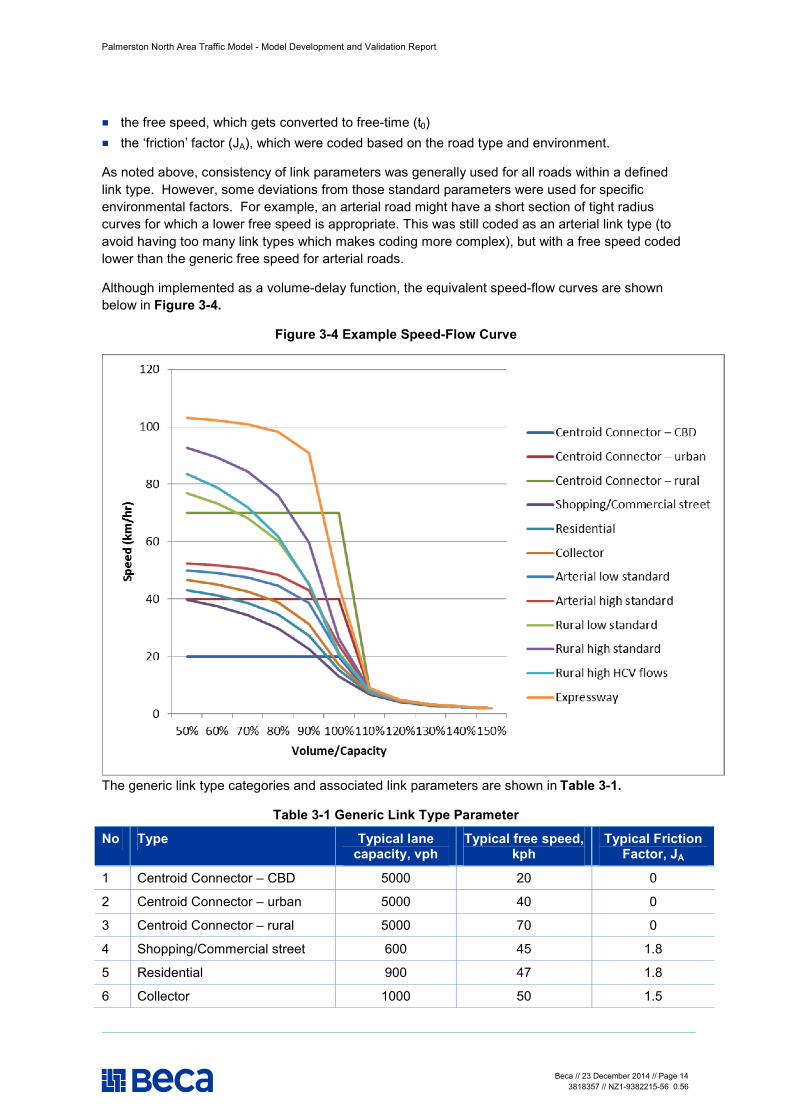
Although implemented as a volume-delay function, the equivalent speed-flow curves are shown below in Figure 3-4.
Figure 3-4 Example Speed-Flow Curve
The generic link type categories and associated link parameters are shown in Table 3-1.
Table 3-1 Generic Link Type Parameter
No Type Typical lane capacity, vph
Typical free speed, kph
Typical Friction Factor, JA
1 Centroid Connector – CBD 5000 20 0
2 Centroid Connector – urban 5000 40 0
3 Centroid Connector – rural 5000 70 0
4 Shopping/Commercial street 600 45 1.8
5 Residential 900 47 1.8
6 Collector 1000 50 1.5
Palmerston North Area Traffic Model - Model Development and Validation Report
Beca // 23 December 2014 // Page 15 3818357 // NZ1-9382215-56 0.56
No Type Typical lane capacity, vph
Typical free speed, kph
Typical Friction Factor, JA
7 Arterial low standard 1250 52 1
8 Arterial high standard 1450 54 0.8
9 Rural low standard 1200 85 1.5
10 Rural high standard 1500 100 1.2
11 Rural high HCV flows 1100 95 1.6
12 Expressway 1800 105 0.3
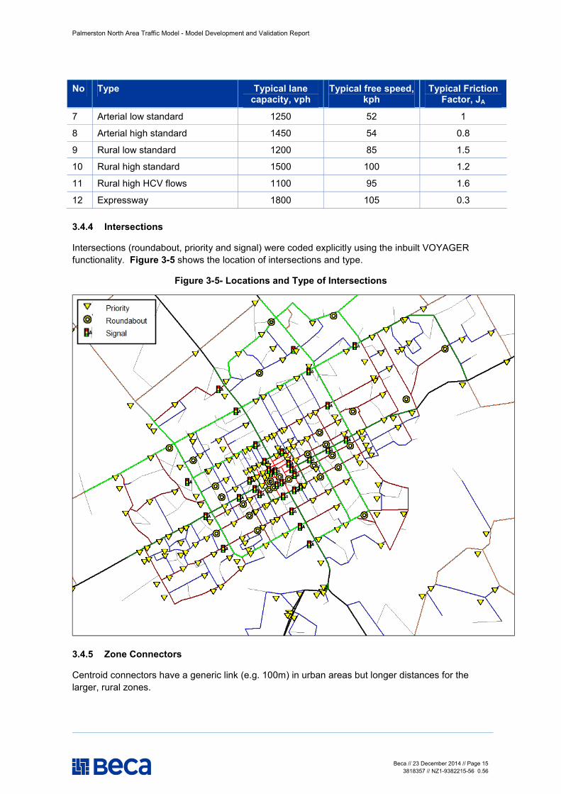
3.4.4 Intersections
Intersections (roundabout, priority and signal) were coded explicitly using the inbuilt VOYAGER functionality. Figure 3-5 shows the location of intersections and type.
Figure 3-5- Locations and Type of Intersections
3.4.5 Zone Connectors
Centroid connectors have a generic link (e.g. 100m) in urban areas but longer distances for the larger, rural zones.

Palmerston North Area Traffic Model - Model Development and Validation Report
Beca // 23 December 2014 // Page 16 3818357 // NZ1-9382215-56 0.56
Centroid connectors use fixed-speeds rather than speed-flow functions because they do not represent real roads for which speed and capacities can be assessed. However, higher speeds were used for longer-distance connectors, such as in rural areas.
3.5 Base Year and Time Periods
The base model year is 2013, using 2013 census land use data and network representation, and calibrated/validated to 2013 traffic data.
The model represents a ‘typical’ weekday, outside the summer holiday period. Peak period models were developed to represent the weekday AM, Interpeak and PM peak periods.
The effect of schools and the university mean that traffic conditions during summer periods are different than the rest of the year. Subsequently, the model represents the ‘academic year’. Traffic data from December and January was therefore not used as an input, or for calibration/validation except in exceptional circumstances. Although the tertiary term does not start until closer to March, the schools are well underway so February is included. Similarly, November was included even though some tertiary students may be finishing and some secondary students would have altered trip patterns due to external exams. To remove February and November would mean excluding an extensive amount of useful count data and also make the model representative of a much shorter part of a year.
The model therefore represents February-November (inclusive).
Three key items were considered in defining time periods:
n To include similar dominant trip types (e.g. commuting) together. This would suggest reasonably long peak periods (e.g. 2-hours);
n The need to represent the peak traffic periods. This would suggest fairly short time periods that represented the true peak rather than being averaged across a long period (which would dampen the true peak effects); and
n Although the demand models can represent any defined period, the assignment models need to operate with 1-hour flows.
To address these somewhat contradictory objectives, different time periods are defined for the demand and assignment models as follows:
n The demand models (which create trip matrices), cover 2-hour peak periods to capture similar trip types. The use of 2-hour demand periods also assists easier comparison of model parameters with other models, most of which use 2-hour periods; and
n The assignment models are 1-hour peak period models. Importantly, these represent the peak within the demand periods, rather than the average of the demand periods.
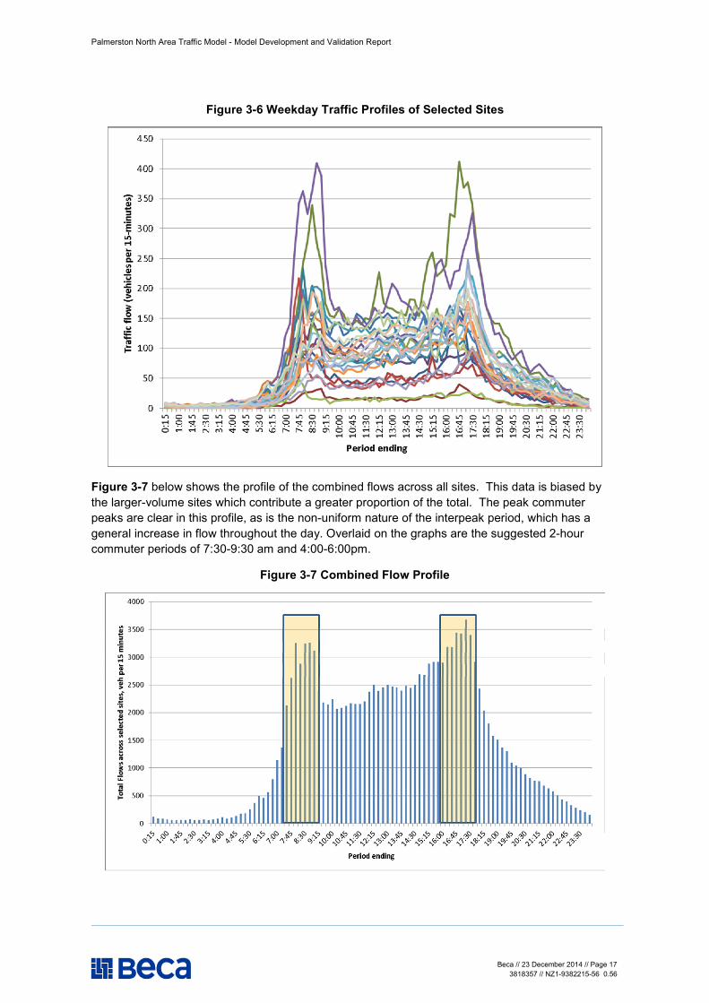
The time periods were selected by analysis of a selection of traffic count data. Thirteen sites were selected across the study area and the 15-minute traffic profiles analysed. Twelve of those sites had data for each direction while one had only combined 2-way data. Overall this gave 25 directional profiles. The locations of these counts are shown in Figure 2-1 with black colour. Figure 3-6 below shows the weekday profile of all 25 sites. This data indicates both large variations in the traffic flows but also variations in the shape of the peak profiles.
Palmerston North Area Traffic Model - Model Development and Validation Report
Beca // 23 December 2014 // Page 17 3818357 // NZ1-9382215-56 0.56
Figure 3-6 Weekday Traffic Profiles of Selected Sites
Figure 3-7 below shows the profile of the combined flows across all sites. This data is biased by the larger-volume sites which contribute a greater proportion of the total. The peak commuter peaks are clear in this profile, as is the non-uniform nature of the interpeak period, which has a general increase in flow throughout the day. Overlaid on the graphs are the suggested 2-hour commuter periods of 7:30-9:30 am and 4:00-6:00pm.
Figure 3-7 Combined Flow Profile
Palmerston North Area Traffic Model - Model Development and Validation Report
Beca // 23 December 2014 // Page 18 3818357 // NZ1-9382215-56 0.56
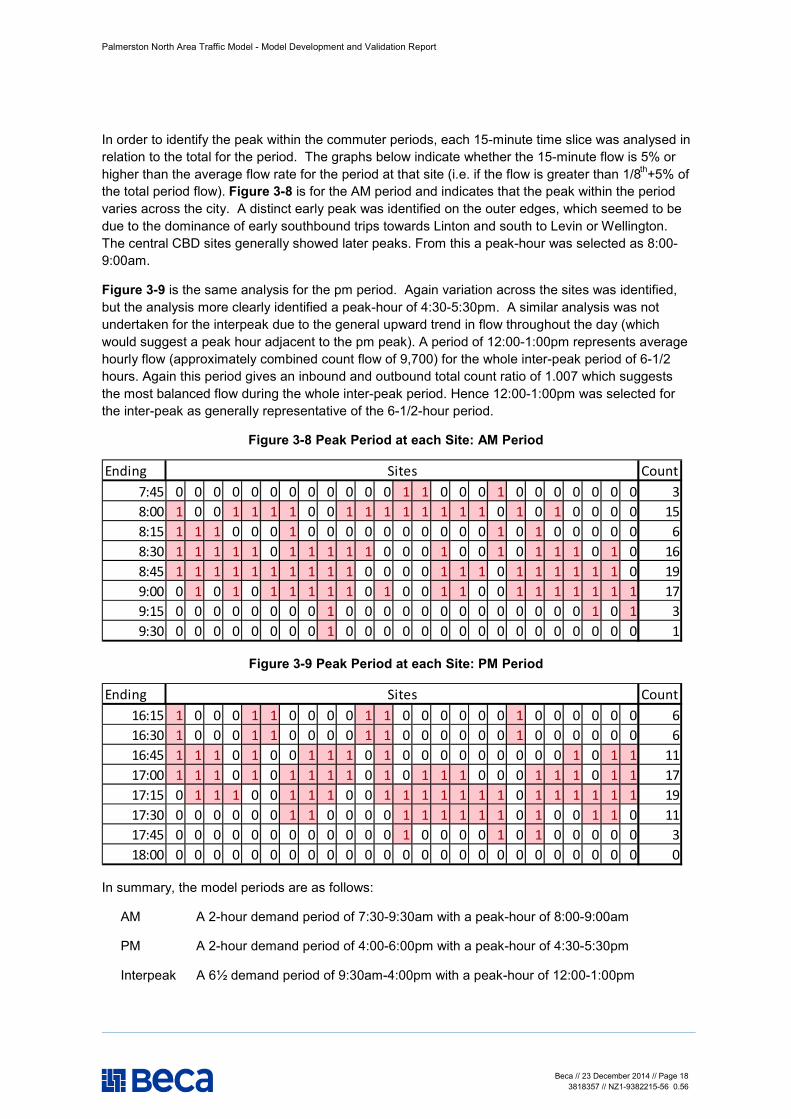
In order to identify the peak within the commuter periods, each 15-minute time slice was analysed in relation to the total for the period. The graphs below indicate whether the 15-minute flow is 5% or higher than the average flow rate for the period at that site (i.e. if the flow is greater than 1/8th+5% of the total period flow). Figure 3-8 is for the AM period and indicates that the peak within the period varies across the city. A distinct early peak was identified on the outer edges, which seemed to be due to the dominance of early southbound trips towards Linton and south to Levin or Wellington. The central CBD sites generally showed later peaks. From this a peak-hour was selected as 8:00-9:00am.
Figure 3-9 is the same analysis for the pm period. Again variation across the sites was identified, but the analysis more clearly identified a peak-hour of 4:30-5:30pm. A similar analysis was not undertaken for the interpeak due to the general upward trend in flow throughout the day (which would suggest a peak hour adjacent to the pm peak). A period of 12:00-1:00pm represents average hourly flow (approximately combined count flow of 9,700) for the whole inter-peak period of 6-1/2 hours. Again this period gives an inbound and outbound total count ratio of 1.007 which suggests the most balanced flow during the whole inter-peak period. Hence 12:00-1:00pm was selected for the inter-peak as generally representative of the 6-1/2-hour period.
Figure 3-8 Peak Period at each Site: AM Period
Ending Count7:45 0 0 0 0 0 0 0 0 0 0 0 0 1 1 0 0 0 1 0 0 0 0 0 0 0 38:00 1 0 0 1 1 1 1 0 0 1 1 1 1 1 1 1 1 0 1 0 1 0 0 0 0 158:15 1 1 1 0 0 0 1 0 0 0 0 0 0 0 0 0 0 1 0 1 0 0 0 0 0 68:30 1 1 1 1 1 0 1 1 1 1 1 0 0 0 1 0 0 1 0 1 1 1 0 1 0 168:45 1 1 1 1 1 1 1 1 1 1 0 0 0 0 1 1 1 0 1 1 1 1 1 1 0 199:00 0 1 0 1 0 1 1 1 1 1 0 1 0 0 1 1 0 0 1 1 1 1 1 1 1 179:15 0 0 0 0 0 0 0 0 1 0 0 0 0 0 0 0 0 0 0 0 0 0 1 0 1 39:30 0 0 0 0 0 0 0 0 1 0 0 0 0 0 0 0 0 0 0 0 0 0 0 0 0 1
Sites
Figure 3-9 Peak Period at each Site: PM Period
Ending Count16:15 1 0 0 0 1 1 0 0 0 0 1 1 0 0 0 0 0 0 1 0 0 0 0 0 0 616:30 1 0 0 0 1 1 0 0 0 0 1 1 0 0 0 0 0 0 1 0 0 0 0 0 0 616:45 1 1 1 0 1 0 0 1 1 1 0 1 0 0 0 0 0 0 0 0 0 1 0 1 1 1117:00 1 1 1 0 1 0 1 1 1 1 0 1 0 1 1 1 0 0 0 1 1 1 0 1 1 1717:15 0 1 1 1 0 0 1 1 1 0 0 1 1 1 1 1 1 1 0 1 1 1 1 1 1 1917:30 0 0 0 0 0 0 1 1 0 0 0 0 1 1 1 1 1 1 0 1 0 0 1 1 0 1117:45 0 0 0 0 0 0 0 0 0 0 0 0 1 0 0 0 0 1 0 1 0 0 0 0 0 318:00 0 0 0 0 0 0 0 0 0 0 0 0 0 0 0 0 0 0 0 0 0 0 0 0 0 0
Sites
In summary, the model periods are as follows:
AM A 2-hour demand period of 7:30-9:30am with a peak-hour of 8:00-9:00am
PM A 2-hour demand period of 4:00-6:00pm with a peak-hour of 4:30-5:30pm
Interpeak A 6½ demand period of 9:30am-4:00pm with a peak-hour of 12:00-1:00pm
Palmerston North Area Traffic Model - Model Development and Validation Report
Beca // 23 December 2014 // Page 19 3818357 // NZ1-9382215-56 0.56
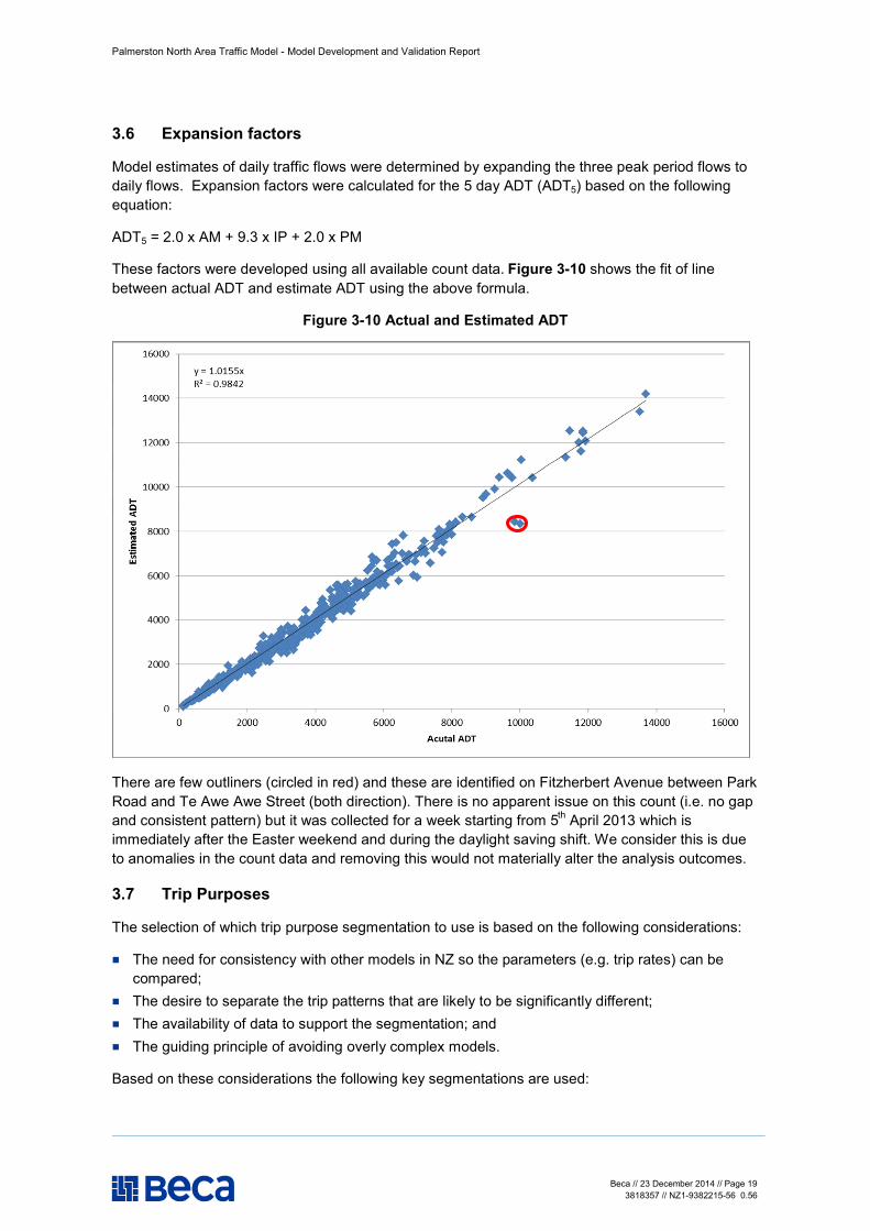
3.6 Expansion factors
Model estimates of daily traffic flows were determined by expanding the three peak period flows to daily flows. Expansion factors were calculated for the 5 day ADT (ADT5) based on the following equation:
ADT5 = 2.0 x AM + 9.3 x IP + 2.0 x PM
These factors were developed using all available count data. Figure 3-10 shows the fit of line between actual ADT and estimate ADT using the above formula.
Figure 3-10 Actual and Estimated ADT
There are few outliners (circled in red) and these are identified on Fitzherbert Avenue between Park Road and Te Awe Awe Street (both direction). There is no apparent issue on this count (i.e. no gap and consistent pattern) but it was collected for a week starting from 5th April 2013 which is immediately after the Easter weekend and during the daylight saving shift. We consider this is due to anomalies in the count data and removing this would not materially alter the analysis outcomes.
3.7 Trip Purposes
The selection of which trip purpose segmentation to use is based on the following considerations:
n The need for consistency with other models in NZ so the parameters (e.g. trip rates) can be compared;
n The desire to separate the trip patterns that are likely to be significantly different; n The availability of data to support the segmentation; and n The guiding principle of avoiding overly complex models.
Based on these considerations the following key segmentations are used:
Palmerston North Area Traffic Model - Model Development and Validation Report
Beca // 23 December 2014 // Page 20 3818357 // NZ1-9382215-56 0.56
n Home Based Work (HBW). These commuter trips are distinct from other trips and there is good information available through census Journey To Work data;
n Home Based Education (HBE). Again these trips are distinct in their destinations and timing of travel, and are especially important in regard to the influence of Massey University;
n Heavy Commercial Vehicles (HCV). These are distinct in terms of the vehicle characteristics and there is a desire to be able to identify forecasts for such vehicles separately from light vehicles. Although it is a vehicle class rather than a trip purpose, the vast majority of truck movements are for commercial purposes. Information for this class of vehicles is available in both traffic counts and from the eruc GPS data;
n Employers Business (EB). Although these are not distinguishable in the traffic count data, it can be useful to estimate these trips separately for economic analysis and most other models include model parameters for this purpose. These are non-home based trips;
n Home Based Shopping Trips (HBS). These trips are distinguished by the time of travel and typical parameters can be sourced as most similar models include this segmentation;
n Home Based Other trips (HBO). This purpose is common to most models of this type and generally has the most number of trips as it is a kind of ‘catch-all’ of all other trips. These are normally modelled separately for home-based and non-home based;
n Non-Home Based Other trips (NHBO).
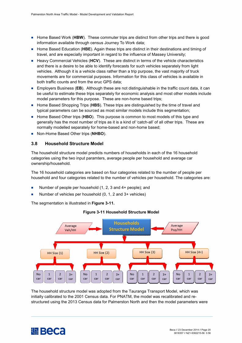
3.8 Household Structure Model
The household structure model predicts numbers of households in each of the 16 household categories using the two input paramters, average people per household and average car ownership/household.
The 16 household categories are based on four categories related to the number of people per household and four categories related to the number of vehicles per household. The categories are:
n Number of people per household (1, 2, 3 and 4+ people); and n Number of vehicles per household (0, 1, 2 and 3+ vehicles)
The segmentation is illustrated in Figure 3-11.
Figure 3-11 Household Structure Model
The household structure model was adopted from the Tauranga Transport Model, which was initially calibrated to the 2001 Census data. For PNATM, the model was recalibrated and re-structured using the 2013 Census data for Palmerston North and then the model parameters were
Palmerston North Area Traffic Model - Model Development and Validation Report
Beca // 23 December 2014 // Page 21 3818357 // NZ1-9382215-56 0.56
re-estimated. Due to the privacy issue, 16 household category information was available only at CAU level and used for the recalibration.
The model works in two steps; first it estimates the total numbers for household for each household size category, then it splits into different level of car ownership within each household size.
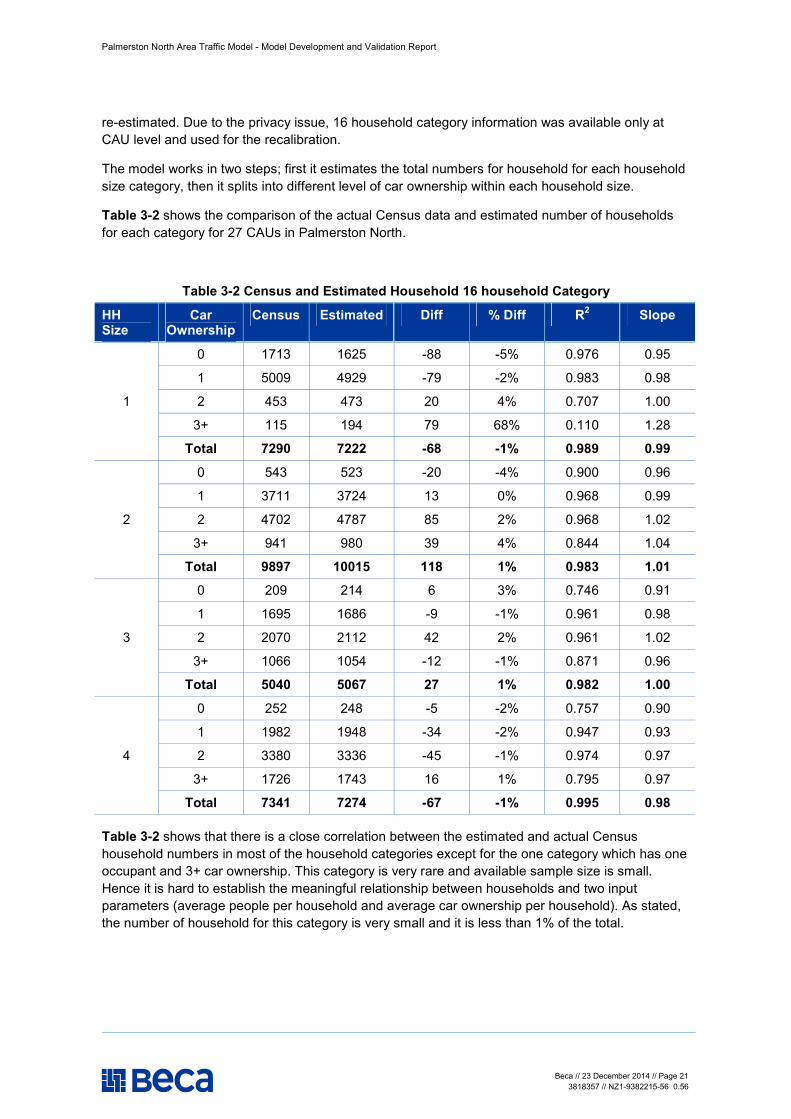
Table 3-2 shows the comparison of the actual Census data and estimated number of households for each category for 27 CAUs in Palmerston North.
Table 3-2 Census and Estimated Household 16 household Category
HH Size
Car Ownership
Census Estimated Diff % Diff R2 Slope
1
0 1713 1625 -88 -5% 0.976 0.95
1 5009 4929 -79 -2% 0.983 0.98
2 453 473 20 4% 0.707 1.00
3+ 115 194 79 68% 0.110 1.28
Total 7290 7222 -68 -1% 0.989 0.99
2
0 543 523 -20 -4% 0.900 0.96
1 3711 3724 13 0% 0.968 0.99
2 4702 4787 85 2% 0.968 1.02
3+ 941 980 39 4% 0.844 1.04
Total 9897 10015 118 1% 0.983 1.01
3
0 209 214 6 3% 0.746 0.91
1 1695 1686 -9 -1% 0.961 0.98
2 2070 2112 42 2% 0.961 1.02
3+ 1066 1054 -12 -1% 0.871 0.96
Total 5040 5067 27 1% 0.982 1.00
4
0 252 248 -5 -2% 0.757 0.90
1 1982 1948 -34 -2% 0.947 0.93
2 3380 3336 -45 -1% 0.974 0.97
3+ 1726 1743 16 1% 0.795 0.97
Total 7341 7274 -67 -1% 0.995 0.98
Table 3-2 shows that there is a close correlation between the estimated and actual Census household numbers in most of the household categories except for the one category which has one occupant and 3+ car ownership. This category is very rare and available sample size is small. Hence it is hard to establish the meaningful relationship between households and two input parameters (average people per household and average car ownership per household). As stated, the number of household for this category is very small and it is less than 1% of the total.

Palmerston North Area Traffic Model - Model Development and Validation Report
Beca // 23 December 2014 // Page 22 3818357 // NZ1-9382215-56 0.56
4 Trip Generation Model
The main inputs to the traffic generation model were from the 2013 census land use data which includes total population, households, employment, primary, secondary and young adult age. In addition, school roll information for primary, secondary and tertiary students was used.
4.1 Base Year Land Use Data
The household and employment data was obtained from the 2013 census and was used directly in the development of the base year model. The following processing was undertaken for the base demographic data:
n Household data were aggregated to the model travel zones from meshblock level; n Employment data (Retail, Agriculture, Industry, Education and Services) was also generated
from Census 2013 using ANZSIC96 classification. Due to privacy issues, this data at meshblock level is generally not available for each employment category. Hence the proportion of each employment category was calculated at CAU level (for each CAU) then applied to the meshblock employment total to estimate the employment splits. Then they are aggregated to the model travel zones.
n School enrolment data was provided by PNCC and aggregated to the model travel zones; n The population of primary and secondary school age was determined from the census data. Due
to the privacy issue, a similar process (as in the employment data) was undertaken to estimate the school age at meshblock level and then aggregated to the model travel zones.
The land use data used for PNATM in the base year are as follows:
n Population – 99,609 people; n Households – 36,993 homes; n Total numbers of car – 59,966 cars; n Retail employment – 10,698 employees; n Agriculture employment – 1,625 employees; n Industrial employment – 7,515 employees; n Education employment – 5,028 employees; n Service employment – 18,428 employees; n Total employment – 43,293 employees; n Primary + Secondary school age (5-17.5yr) – 18,926 (19% of total population) n Young Adult, Tertiary (17.5-24yr) – 11,328 (11% of total population) n Primary school roll – 10,648 students; n Secondary school roll – 7,380 students; and n Tertiary school roll – 14,721 students.
4.2 Trip Production/Attraction Models
The trip generation model was developed in a spreadsheet for greater transparency and manipulation of inputs. The model used the outputs from the household structure model and trip productions are a function of 16 household categories and their related trip rates. Trips rates were initially adopted from the Tauranga Transport Model and then further recalibrated to local count data and census data. The general form is as follows:
Palmerston North Area Traffic Model - Model Development and Validation Report
Beca // 23 December 2014 // Page 23 3818357 // NZ1-9382215-56 0.56
n The HBW, HBS and HBO production models was based on household data with attraction models based on employment data;
n The HCV use the same trip rates for production and attractions. These are based primarily on employment data but with a low trip rate was also applied to household numbers (to represent home deliveries, tradesmen etc);
n The NHBO and EB also use the same trip rates for production and attraction. These models are based on both employment and household data. The production models is based on household data, however these are only used to control the total number of such trips made. Then in the attraction model, employment data was used to estimate the trip then adjusted to match the total numbers of trips predicted by the production model;
n The HBE purpose is based on separate production/attraction models for primary, secondary and tertiary education. The productions are estimated from the population in each zone estimated to be of primary /secondary and tertiary age. Then attractions are based on the school rolls.
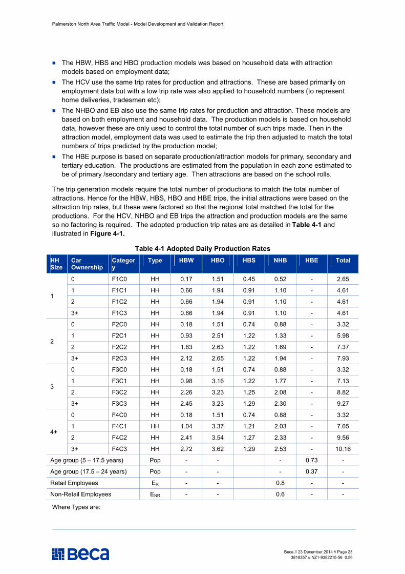
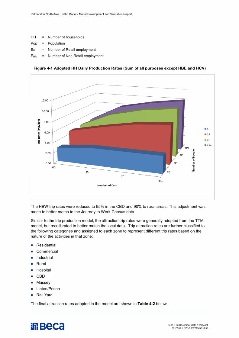
The trip generation models require the total number of productions to match the total number of attractions. Hence for the HBW, HBS, HBO and HBE trips, the initial attractions were based on the attraction trip rates, but these were factored so that the regional total matched the total for the productions. For the HCV, NHBO and EB trips the attraction and production models are the same so no factoring is required. The adopted production trip rates are as detailed in Table 4-1 and illustrated in Figure 4-1.
Table 4-1 Adopted Daily Production Rates HH Size
Car Ownership
Category
Type HBW HBO HBS NHB HBE Total
1
0 F1C0 HH 0.17 1.51 0.45 0.52 - 2.65
1 F1C1 HH 0.66 1.94 0.91 1.10 - 4.61
2 F1C2 HH 0.66 1.94 0.91 1.10 - 4.61
3+ F1C3 HH 0.66 1.94 0.91 1.10 - 4.61
2
0 F2C0 HH 0.18 1.51 0.74 0.88 - 3.32
1 F2C1 HH 0.93 2.51 1.22 1.33 - 5.98
2 F2C2 HH 1.83 2.63 1.22 1.69 - 7.37
3+ F2C3 HH 2.12 2.65 1.22 1.94 - 7.93
3
0 F3C0 HH 0.18 1.51 0.74 0.88 - 3.32
1 F3C1 HH 0.98 3.16 1.22 1.77 - 7.13
2 F3C2 HH 2.26 3.23 1.25 2.08 - 8.82
3+ F3C3 HH 2.45 3.23 1.29 2.30 - 9.27
4+
0 F4C0 HH 0.18 1.51 0.74 0.88 - 3.32
1 F4C1 HH 1.04 3.37 1.21 2.03 - 7.65
2 F4C2 HH 2.41 3.54 1.27 2.33 - 9.56
3+ F4C3 HH 2.72 3.62 1.29 2.53 - 10.16
Age group (5 – 17.5 years) Pop - - - 0.73 -
Age group (17.5 – 24 years) Pop - - - 0.37 -
Retail Employees ER - - 0.8 - -
Non-Retail Employees ENR - - 0.6 - -
Where Types are:
Palmerston North Area Traffic Model - Model Development and Validation Report
Beca // 23 December 2014 // Page 24 3818357 // NZ1-9382215-56 0.56
HH = Number of households
Pop = Population
ER = Number of Retail employment
ENR = Number of Non-Retail employment
Figure 4-1 Adopted HH Daily Production Rates (Sum of all purposes except HBE and HCV)
The HBW trip rates were reduced to 95% in the CBD and 90% to rural areas. This adjustment was made to better match to the Journey to Work Census data.
Similar to the trip production model, the attraction trip rates were generally adopted from the TTM model, but recalibrated to better match the local data. Trip attraction rates are further classified to the following categories and assigned to each zone to represent different trip rates based on the nature of the activities in that zone:
n Residential n Commercial n Industrial n Rural n Hospital n CBD n Massey n Linton/Prison n Rail Yard
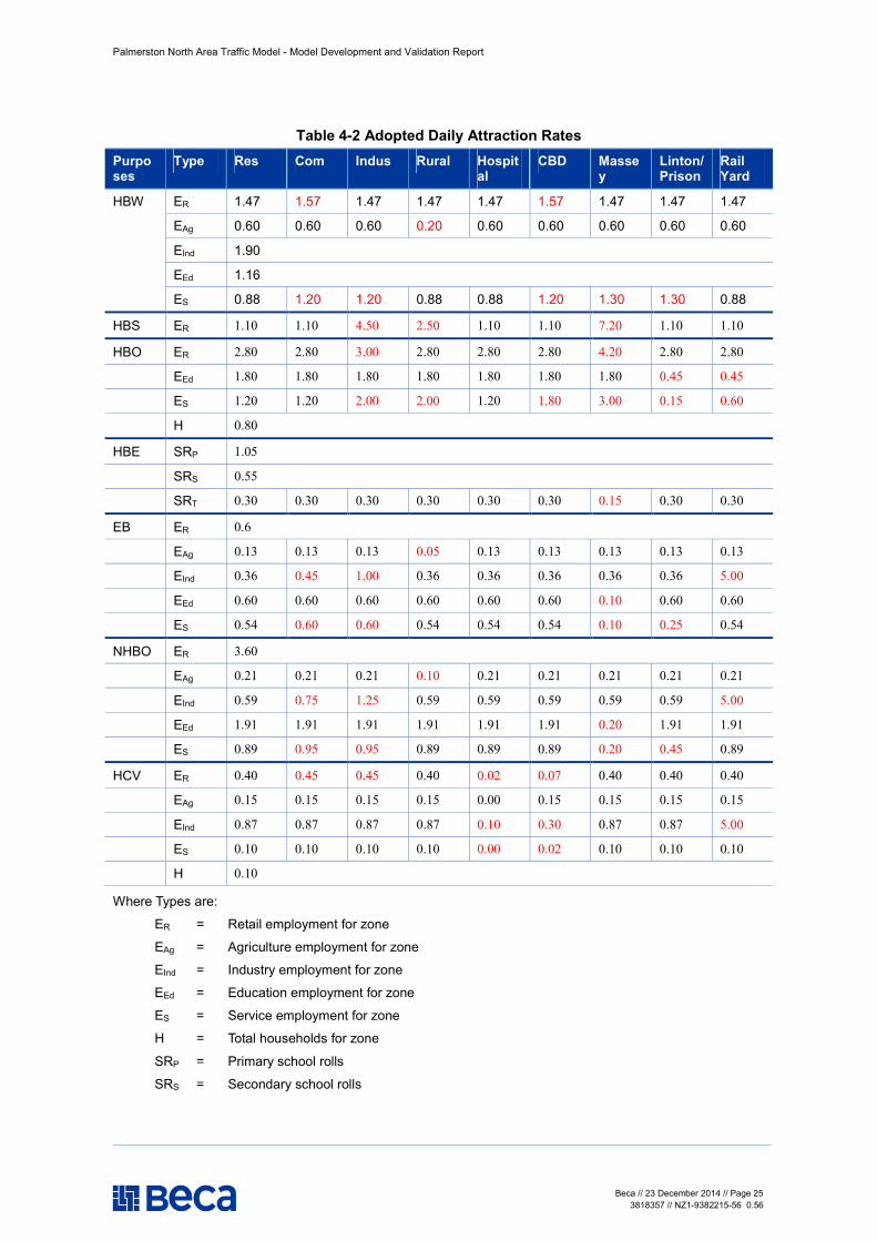
The final attraction rates adopted in the model are shown in Table 4-2 below.
Palmerston North Area Traffic Model - Model Development and Validation Report
Beca // 23 December 2014 // Page 25 3818357 // NZ1-9382215-56 0.56
Table 4-2 Adopted Daily Attraction Rates Purposes
Type Res Com Indus Rural Hospital
CBD Massey
Linton/Prison
Rail Yard
HBW ER 1.47 1.57 1.47 1.47 1.47 1.57 1.47 1.47 1.47
EAg 0.60 0.60 0.60 0.20 0.60 0.60 0.60 0.60 0.60
EInd 1.90
EEd 1.16
ES 0.88 1.20 1.20 0.88 0.88 1.20 1.30 1.30 0.88
HBS ER 1.10 1.10 4.50 2.50 1.10 1.10 7.20 1.10 1.10
HBO ER 2.80 2.80 3.00 2.80 2.80 2.80 4.20 2.80 2.80
EEd 1.80 1.80 1.80 1.80 1.80 1.80 1.80 0.45 0.45
ES 1.20 1.20 2.00 2.00 1.20 1.80 3.00 0.15 0.60
H 0.80
HBE SRP 1.05
SRS 0.55
SRT 0.30 0.30 0.30 0.30 0.30 0.30 0.15 0.30 0.30
EB ER 0.6
EAg 0.13 0.13 0.13 0.05 0.13 0.13 0.13 0.13 0.13
EInd 0.36 0.45 1.00 0.36 0.36 0.36 0.36 0.36 5.00
EEd 0.60 0.60 0.60 0.60 0.60 0.60 0.10 0.60 0.60
ES 0.54 0.60 0.60 0.54 0.54 0.54 0.10 0.25 0.54
NHBO ER 3.60
EAg 0.21 0.21 0.21 0.10 0.21 0.21 0.21 0.21 0.21
EInd 0.59 0.75 1.25 0.59 0.59 0.59 0.59 0.59 5.00
EEd 1.91 1.91 1.91 1.91 1.91 1.91 0.20 1.91 1.91
ES 0.89 0.95 0.95 0.89 0.89 0.89 0.20 0.45 0.89
HCV ER 0.40 0.45 0.45 0.40 0.02 0.07 0.40 0.40 0.40
EAg 0.15 0.15 0.15 0.15 0.00 0.15 0.15 0.15 0.15
EInd 0.87 0.87 0.87 0.87 0.10 0.30 0.87 0.87 5.00
ES 0.10 0.10 0.10 0.10 0.00 0.02 0.10 0.10 0.10
H 0.10
Where Types are:
ER = Retail employment for zone
EAg = Agriculture employment for zone
EInd = Industry employment for zone
EEd = Education employment for zone
ES = Service employment for zone
H = Total households for zone
SRP = Primary school rolls
SRS = Secondary school rolls
Palmerston North Area Traffic Model - Model Development and Validation Report
Beca // 23 December 2014 // Page 26 3818357 // NZ1-9382215-56 0.56
Resulting attraction trips were adjusted to match the trip production totals. Adjustment factors are provided in Table 4-3.
Table 4-3 Adjustment Factors for Attraction Trips HBW HBS HBO HBE NHB-EB NHB-O
1.01 0.96 0.96 1.00 0.98 0.98
4.3 External Models
Two types of ‘external’ trips are used in the model as follows:
n External-to-external (‘through’) trips; n External-internal or internal-external trips; and
4.3.1 Through Traffic
Two sources of data have been used to develop an external to external matrix, namely commercial GPS and Bluetooth survey data. The HCV through matrix was generated from the commercial GPS data which includes all external zones. From the Bluetooth survey, an all vehicle matrix was developed but this is only for the selected four external zones (4x4 matrix) where Bluetooth units were deployed. Details of the Bluetooth survey are documented and provided in Appendix A.
To develop a complete all vehicle external matrix, the Bluetooth data had been used for four external zones. The total vehicle matrix heading to/from the remaining external zones was estimated by expanding the commercial GPS matrix by the HCV percentage at each external entry point.
The estimated all vehicles through matrix is 2,600 trips per day which is approximately 1% of the total vehicle matrix of the model.
4.3.2 External-Internal Trips
The external-internal (and reverse) trips were included directly in the generation/distribution models. Trip ends (in 24-hour production/attraction format) were developed by using the through traffic matrix and external count data. This gives trip ends at each external point by HCV and Light vehicles. The external trip ends for the HBW purpose were derived from the census JTW data. The remaining trip purposes are segmented using the global model split factors.
The internal-external trips, which represent trips entering or leaving the model, were then included in the trip generation spreadsheet to produce trip ends for the distribution model.
4.4 Airport Model
The initial analysis showed that there was very weak correlation between the land use activities and trip generations at airport. To get the appropriate generation from the airport, the trip rates are needed to be approximately 10 times higher than those of other normal zones. Hence trip generation from the airport would be highly sensitive to land use changes. This could create potential issues in future year models where changes in land use are assessed.
Hence, in the trip generation model, land use activities (mainly employment) in the airport zone were not used. Instead the trip ends were generated based on the special traffic count (at the entrance of the airport) and then these were included in the trip generation spreadsheet (similar to external to internal trips).
Palmerston North Area Traffic Model - Model Development and Validation Report
Beca // 23 December 2014 // Page 27 3818357 // NZ1-9382215-56 0.56
5 Trip Distribution Model
5.1 Model Form
The distribution model allocates zonal trip productions to destination zones. A doubly-constrained gravity model was used for this purpose, operated at a 24-hour level, which is a typical model form. The model form is as follows:
ijijjijiij KCFAPbaT )(=
where: Tij = Trips from zone I to zone j
Pi = Productions form zone I
Aj = Attractions to zone j
F(Cij) = A cost deterrence (impedance) function
Cij = the generalised cost between zone i and zone j
ai, bj = row and column balancing factors
Kij = area-specific adjustment factors
5.2 Impedance Function
The impedance function controls the sensitivity to trip costs and was defined as follows:
( )ijxCij eCF =)(
where: x is calibration constants and C is the generalised cost described above.
5.3 Generalised Cost
The defined generalised cost function included time, Vehicle Operating Costs (VOC) and toll costs. The VOC and toll monetary costs were converted to generalised minutes using Values of Time (VoT). The VoT was adopted form the HBC model. The generalised cost was hence:
ijijijij TOLLTLDISTDTIMETGC ×+×+×=
Where:
GCij = generalised cost of travel from zone i to zone j, used in the distribution model
T = weight on time
TIMEij = travel time (minutes) between zone i and zone j
D = weight on travel distance, representing a vehicle operating cost
DISTij = travel distance (km) between zone i and zone j
TL = weight applied to monetary toll
TOLLij = toll cost (cents), between zone i and zone j
Palmerston North Area Traffic Model - Model Development and Validation Report
Beca // 23 December 2014 // Page 28 3818357 // NZ1-9382215-56 0.56
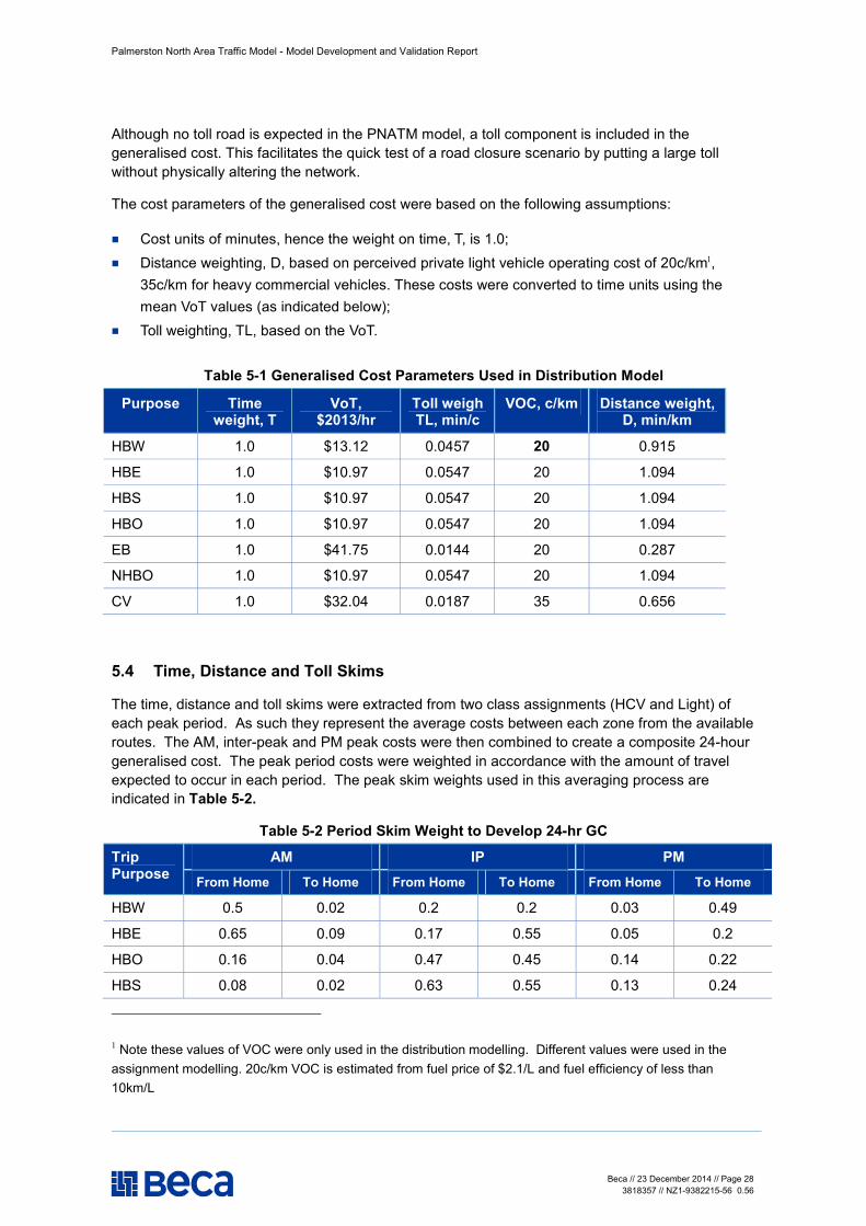
Although no toll road is expected in the PNATM model, a toll component is included in the generalised cost. This facilitates the quick test of a road closure scenario by putting a large toll without physically altering the network.
The cost parameters of the generalised cost were based on the following assumptions:
n Cost units of minutes, hence the weight on time, T, is 1.0; n Distance weighting, D, based on perceived private light vehicle operating cost of 20c/km1,
35c/km for heavy commercial vehicles. These costs were converted to time units using the mean VoT values (as indicated below);
n Toll weighting, TL, based on the VoT.
Table 5-1 Generalised Cost Parameters Used in Distribution Model
Purpose Time weight, T
VoT, $2013/hr
Toll weigh TL, min/c
VOC, c/km Distance weight, D, min/km
HBW 1.0 $13.12 0.0457 20 0.915
HBE 1.0 $10.97 0.0547 20 1.094
HBS 1.0 $10.97 0.0547 20 1.094
HBO 1.0 $10.97 0.0547 20 1.094
EB 1.0 $41.75 0.0144 20 0.287
NHBO 1.0 $10.97 0.0547 20 1.094
CV 1.0 $32.04 0.0187 35 0.656
5.4 Time, Distance and Toll Skims
The time, distance and toll skims were extracted from two class assignments (HCV and Light) of each peak period. As such they represent the average costs between each zone from the available routes. The AM, inter-peak and PM peak costs were then combined to create a composite 24-hour generalised cost. The peak period costs were weighted in accordance with the amount of travel expected to occur in each period. The peak skim weights used in this averaging process are indicated in Table 5-2.
Table 5-2 Period Skim Weight to Develop 24-hr GC
Trip Purpose
AM IP PM From Home To Home From Home To Home From Home To Home
HBW 0.5 0.02 0.2 0.2 0.03 0.49
HBE 0.65 0.09 0.17 0.55 0.05 0.2
HBO 0.16 0.04 0.47 0.45 0.14 0.22
HBS 0.08 0.02 0.63 0.55 0.13 0.24
1 Note these values of VOC were only used in the distribution modelling. Different values were used in the assignment modelling. 20c/km VOC is estimated from fuel price of $2.1/L and fuel efficiency of less than 10km/L
Palmerston North Area Traffic Model - Model Development and Validation Report
Beca // 23 December 2014 // Page 29 3818357 // NZ1-9382215-56 0.56
Trip Purpose
AM IP PM From Home To Home From Home To Home From Home To Home
EB 0.15 0.58 0.12
NHBO 0.13 0.58 0.14
HCV 0.17 0.51 0.15
5.4.1 Access, Intra-Zonal and External Costs
Intra-zonal costs were set as 50% of the cost to the nearest neighbour zone. External-to-external costs were set to ‘999999’ to exclude any such trip making in the distribution models.
5.5 Demand/Supply Convergence
The demand model requires updating of the travel costs as the trip demands are created. This requires iterations of the gravity and assignment models until satisfactory convergence is achieved. Maximum iteration was set to ten and a convergence criterion is 0.1% of changes in vehicle cost between current and previous iteration. A cost damping process was also introduced between iterations to speed convergence.
5.6 Calibration of HBW Distribution Model
The impedance functions control distribution of the trips and they are unique based on the geographical layouts of the models. Impedance functions calibrated in other models may not be appropriate for the PNATM. As such a local calibration was undertaken using the JTW census data which is a good data source for travel patterns of commuter (HBW) trips.
It is aware that the JTW data is collected only for the census day and the data may not be a true representation of JTW travel patterns. However, in the lack of other available data, the JTW census data was used for calibration of HBW travel patterns which is a common practice in other similar models.
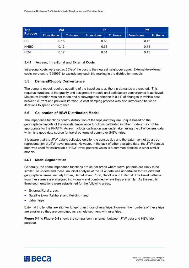
5.6.1 Model Segmentation
Generally, the same impedance functions are set for areas where travel patterns are likely to be similar. To understand these, an initial analysis of the JTW data was undertaken for five different geographical areas; namely Urban, Semi-Urban, Rural, Satellite and External. The travel patterns from these areas are analysed individually and combined where they are similar. As the results, three segmentations were established for the following areas;
n External/Rural areas; n Satellite town (Ashhurst and Feilding); and n Urban trips.
External trip lengths are slighter longer than those of rural trips. However the numbers of these trips are smaller so they are combined as a single segment with rural trips.
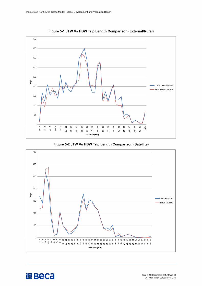
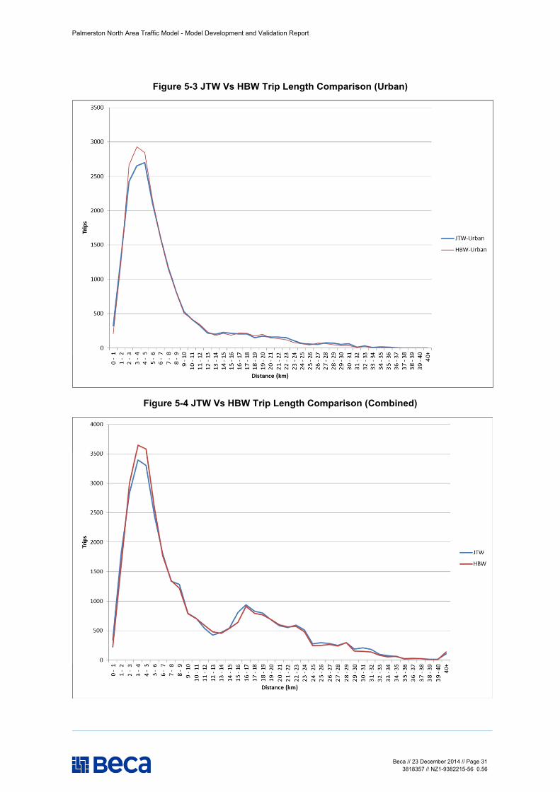
Figure 5-1 to Figure 5-4 shows the comparison trip length between JTW data and HBW trip purpose.
Palmerston North Area Traffic Model - Model Development and Validation Report
Beca // 23 December 2014 // Page 30 3818357 // NZ1-9382215-56 0.56
Figure 5-1 JTW Vs HBW Trip Length Comparison (External/Rural)
Figure 5-2 JTW Vs HBW Trip Length Comparison (Satellite)
Palmerston North Area Traffic Model - Model Development and Validation Report
Beca // 23 December 2014 // Page 31 3818357 // NZ1-9382215-56 0.56
Figure 5-3 JTW Vs HBW Trip Length Comparison (Urban)
Figure 5-4 JTW Vs HBW Trip Length Comparison (Combined)
Palmerston North Area Traffic Model - Model Development and Validation Report
Beca // 23 December 2014 // Page 32 3818357 // NZ1-9382215-56 0.56
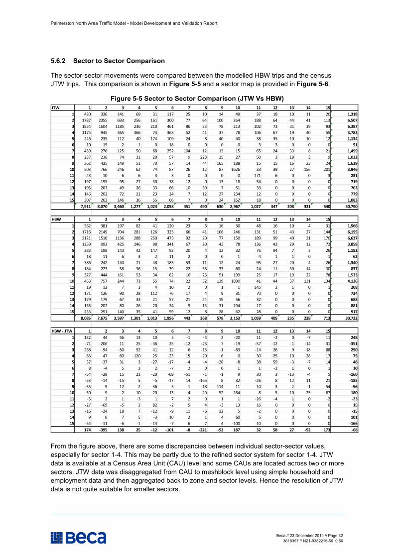
5.6.2 Sector to Sector Comparison
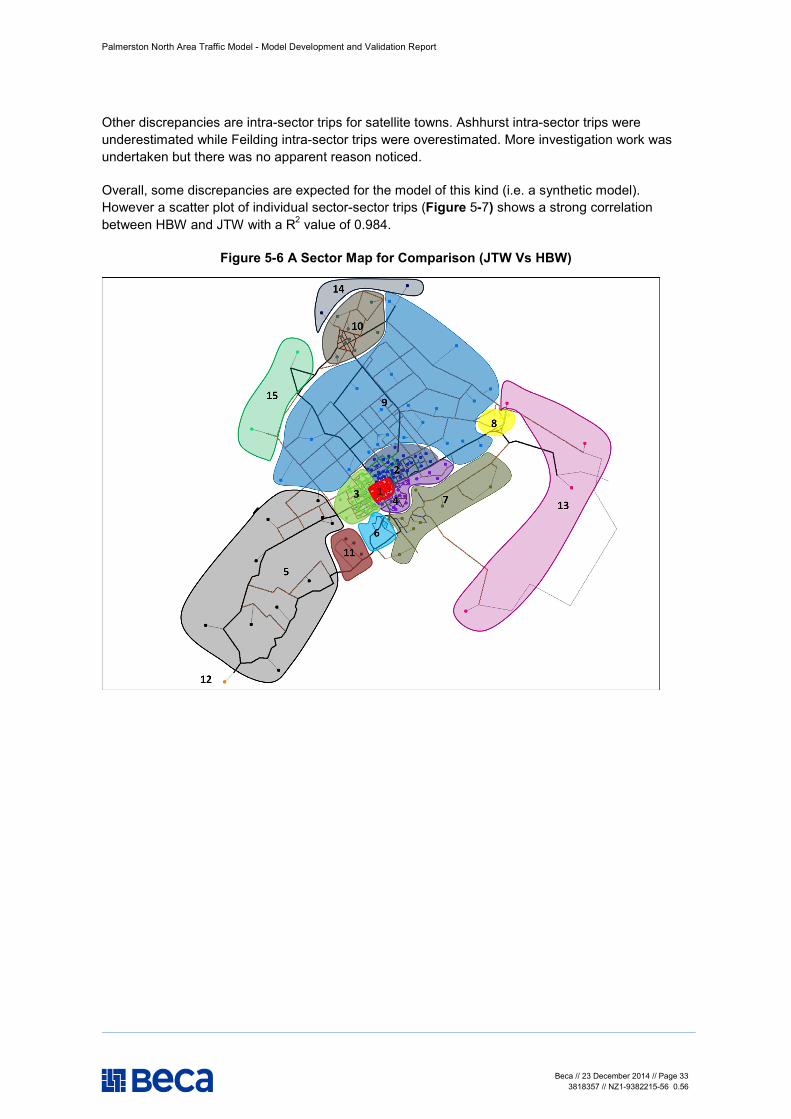
The sector-sector movements were compared between the modelled HBW trips and the census JTW trips. This comparison is shown in Figure 5-5 and a sector map is provided in Figure 5-6.
Figure 5-5 Sector to Sector Comparison (JTW Vs HBW) JTW 1 2 3 4 5 6 7 8 9 10 11 12 13 14 15
1 430 336 141 69 31 117 25 10 14 49 37 18 10 11 20 1,3182 1787 2355 693 256 161 300 77 64 100 264 188 64 44 41 113 6,5073 1854 1604 1185 236 210 461 86 33 78 213 202 73 31 39 83 6,3874 1175 945 365 366 73 363 52 41 37 78 106 67 19 40 55 3,7835 246 235 112 40 174 109 24 8 40 40 38 35 10 10 12 1,1346 10 15 2 1 0 18 0 0 0 0 3 3 0 0 0 517 439 270 125 50 68 252 104 12 13 15 65 24 33 8 21 1,4998 237 236 74 31 20 57 9 223 25 27 50 3 18 3 9 1,0229 362 435 149 51 70 57 14 44 165 188 15 15 16 23 24 1,629
10 503 766 246 62 74 87 26 12 87 1626 33 39 27 156 201 3,94611 23 10 6 6 3 3 0 0 0 0 171 6 0 0 3 23112 197 195 95 27 30 78 12 0 13 18 54 0 0 0 0 71913 195 203 49 26 33 66 10 30 7 51 33 0 0 0 0 70314 146 202 72 21 23 24 7 12 27 234 12 0 0 0 0 77915 307 262 146 36 55 66 7 0 24 162 18 0 0 0 0 1,083
7,911 8,070 3,460 1,277 1,024 2,058 451 490 630 2,967 1,027 347 208 331 540 30,790
HBW 1 2 3 4 5 6 7 8 9 10 11 12 13 14 151 562 381 197 82 41 120 23 6 16 30 48 16 10 4 31 1,5662 1716 2149 704 281 126 325 66 41 106 246 131 51 43 27 144 6,1553 2121 1510 1136 288 250 473 92 20 77 150 189 99 40 21 170 6,6374 1259 992 425 246 98 341 67 20 43 78 136 42 29 12 72 3,8585 283 198 143 42 147 93 20 4 12 32 76 94 7 3 26 1,1826 18 11 6 3 2 11 2 0 0 1 4 1 1 0 1 627 386 242 140 71 48 183 53 11 12 24 95 27 20 4 26 1,3408 184 223 58 36 15 39 22 58 33 60 24 11 30 14 30 8379 327 444 161 53 34 62 16 26 51 199 25 17 19 22 78 1,533
10 453 757 244 73 55 74 22 32 139 1890 41 44 37 131 134 4,12611 19 12 7 3 4 10 2 0 1 1 145 2 1 0 1 20812 171 126 90 28 112 76 17 4 9 31 70 0 0 0 0 73413 179 179 67 33 21 57 21 24 19 56 32 0 0 0 0 68814 155 202 80 26 20 34 9 13 31 294 17 0 0 0 0 88115 253 251 140 35 41 59 12 8 28 62 28 0 0 0 0 917
8,085 7,675 3,597 1,301 1,013 1,956 443 268 578 3,153 1,059 405 235 238 713 30,722
HBW - JTW 1 2 3 4 5 6 7 8 9 10 11 12 13 14 151 132 44 56 13 10 3 -1 -4 2 -20 11 -2 0 -7 11 2482 -71 -206 11 25 -36 25 -12 -23 7 -19 -57 -12 -1 -14 31 -3513 268 -94 -50 52 41 12 6 -13 -1 -63 -14 26 9 -18 88 2504 83 47 60 -120 25 -23 15 -20 6 0 30 -25 10 -28 17 755 37 -37 31 3 -27 -17 -4 -4 -28 -8 38 59 -3 -7 14 486 8 -4 5 3 2 -7 2 0 0 1 1 -2 1 0 1 107 -54 -29 15 21 -20 -69 -51 -1 -1 9 30 3 -13 -4 5 -1608 -53 -14 -15 5 -5 -17 14 -165 8 32 -26 8 12 11 21 -1859 -35 9 12 2 -36 5 1 -18 -114 11 10 3 2 -1 54 -96
10 -50 -9 -2 10 -20 -13 -4 20 52 264 8 5 10 -25 -67 18011 -5 2 1 -3 1 7 2 0 1 1 -26 -4 1 0 -2 -2312 -27 -69 -5 2 82 -2 5 4 -3 13 16 0 0 0 0 1513 -16 -24 18 7 -12 -9 11 -6 12 5 -2 0 0 0 0 -1514 9 0 7 5 -3 10 2 1 4 60 5 0 0 0 0 10115 -54 -11 -6 -1 -14 -7 6 7 4 -100 10 0 0 0 0 -166
174 -395 138 25 -12 -101 -8 -221 -52 187 32 58 27 -92 173 -68
From the figure above, there are some discrepancies between individual sector-sector values, especially for sector 1-4. This may be partly due to the refined sector system for sector 1-4. JTW data is available at a Census Area Unit (CAU) level and some CAUs are located across two or more sectors. JTW data was disaggregated from CAU to meshblock level using simple household and employment data and then aggregated back to zone and sector levels. Hence the resolution of JTW data is not quite suitable for smaller sectors.
Palmerston North Area Traffic Model - Model Development and Validation Report
Beca // 23 December 2014 // Page 33 3818357 // NZ1-9382215-56 0.56
Other discrepancies are intra-sector trips for satellite towns. Ashhurst intra-sector trips were underestimated while Feilding intra-sector trips were overestimated. More investigation work was undertaken but there was no apparent reason noticed.
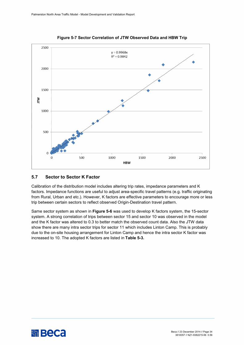
Overall, some discrepancies are expected for the model of this kind (i.e. a synthetic model). However a scatter plot of individual sector-sector trips (Figure 5-7) shows a strong correlation between HBW and JTW with a R2 value of 0.984.
Figure 5-6 A Sector Map for Comparison (JTW Vs HBW)
Palmerston North Area Traffic Model - Model Development and Validation Report
Beca // 23 December 2014 // Page 34 3818357 // NZ1-9382215-56 0.56
Figure 5-7 Sector Correlation of JTW Observed Data and HBW Trip
5.7 Sector to Sector K Factor
Calibration of the distribution model includes altering trip rates, impedance parameters and K factors. Impedance functions are useful to adjust area-specific travel patterns (e.g. traffic originating from Rural, Urban and etc.). However, K factors are effective parameters to encourage more or less trip between certain sectors to reflect observed Origin-Destination travel pattern.
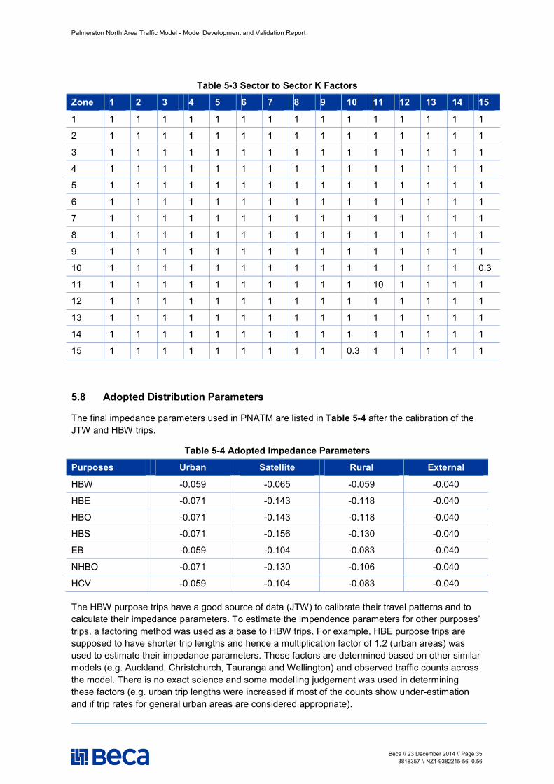
Same sector system as shown in Figure 5-6 was used to develop K factors system, the 15-sector system. A strong correlation of trips between sector 15 and sector 10 was observed in the model and the K factor was altered to 0.3 to better match the observed count data. Also the JTW data show there are many intra sector trips for sector 11 which includes Linton Camp. This is probably due to the on-site housing arrangement for Linton Camp and hence the intra sector K factor was increased to 10. The adopted K factors are listed in Table 5-3.
Palmerston North Area Traffic Model - Model Development and Validation Report
Beca // 23 December 2014 // Page 35 3818357 // NZ1-9382215-56 0.56
Table 5-3 Sector to Sector K Factors
Zone 1 2 3 4 5 6 7 8 9 10 11 12 13 14 15
1 1 1 1 1 1 1 1 1 1 1 1 1 1 1 1
2 1 1 1 1 1 1 1 1 1 1 1 1 1 1 1
3 1 1 1 1 1 1 1 1 1 1 1 1 1 1 1
4 1 1 1 1 1 1 1 1 1 1 1 1 1 1 1
5 1 1 1 1 1 1 1 1 1 1 1 1 1 1 1
6 1 1 1 1 1 1 1 1 1 1 1 1 1 1 1
7 1 1 1 1 1 1 1 1 1 1 1 1 1 1 1
8 1 1 1 1 1 1 1 1 1 1 1 1 1 1 1
9 1 1 1 1 1 1 1 1 1 1 1 1 1 1 1
10 1 1 1 1 1 1 1 1 1 1 1 1 1 1 0.3
11 1 1 1 1 1 1 1 1 1 1 10 1 1 1 1
12 1 1 1 1 1 1 1 1 1 1 1 1 1 1 1
13 1 1 1 1 1 1 1 1 1 1 1 1 1 1 1
14 1 1 1 1 1 1 1 1 1 1 1 1 1 1 1
15 1 1 1 1 1 1 1 1 1 0.3 1 1 1 1 1
5.8 Adopted Distribution Parameters
The final impedance parameters used in PNATM are listed in Table 5-4 after the calibration of the JTW and HBW trips.
Table 5-4 Adopted Impedance Parameters
Purposes Urban Satellite Rural External
HBW -0.059 -0.065 -0.059 -0.040
HBE -0.071 -0.143 -0.118 -0.040
HBO -0.071 -0.143 -0.118 -0.040
HBS -0.071 -0.156 -0.130 -0.040
EB -0.059 -0.104 -0.083 -0.040
NHBO -0.071 -0.130 -0.106 -0.040
HCV -0.059 -0.104 -0.083 -0.040
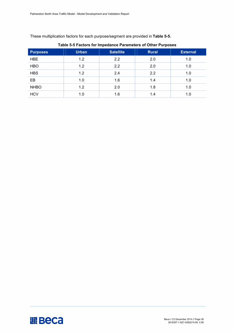
The HBW purpose trips have a good source of data (JTW) to calibrate their travel patterns and to calculate their impedance parameters. To estimate the impendence parameters for other purposes’ trips, a factoring method was used as a base to HBW trips. For example, HBE purpose trips are supposed to have shorter trip lengths and hence a multiplication factor of 1.2 (urban areas) was used to estimate their impedance parameters. These factors are determined based on other similar models (e.g. Auckland, Christchurch, Tauranga and Wellington) and observed traffic counts across the model. There is no exact science and some modelling judgement was used in determining these factors (e.g. urban trip lengths were increased if most of the counts show under-estimation and if trip rates for general urban areas are considered appropriate).
Palmerston North Area Traffic Model - Model Development and Validation Report
Beca // 23 December 2014 // Page 36 3818357 // NZ1-9382215-56 0.56
These multiplication factors for each purpose/segment are provided in Table 5-5.
Table 5-5 Factors for Impedance Parameters of Other Purposes
Purposes Urban Satellite Rural External
HBE 1.2 2.2 2.0 1.0
HBO 1.2 2.2 2.0 1.0
HBS 1.2 2.4 2.2 1.0
EB 1.0 1.6 1.4 1.0
NHBO 1.2 2.0 1.8 1.0
HCV 1.0 1.6 1.4 1.0
Palmerston North Area Traffic Model - Model Development and Validation Report
Beca // 23 December 2014 // Page 37 3818357 // NZ1-9382215-56 0.56
6 Time Period Model
6.1 Model Form
The gravity models output 24-hour Production-Attraction matrices which the Time Period Model converts to peak period Origin-Destination matrices. This is done using time period and direction factors adopted from other models and adjusted to match local count data.
The time period model has two components, firstly a process to determine the peak period demands from the 24-hour demands, and secondly to estimate peak-hour demands from the peak period demands.
The period demands are derived as follows:
24 hour trip matrix in P/A form is pijT
From home trip matrix is p
ijpf
ij TT 21=
To home trip matrix is p
ijjipr
ij TTT ′== 21
21
The matrix for any time period t, is constructed from the formula:
prij
prt
pfij
pft
pijt TTT ×Ρ+×Ρ=
6.2 Period and Direction Factors
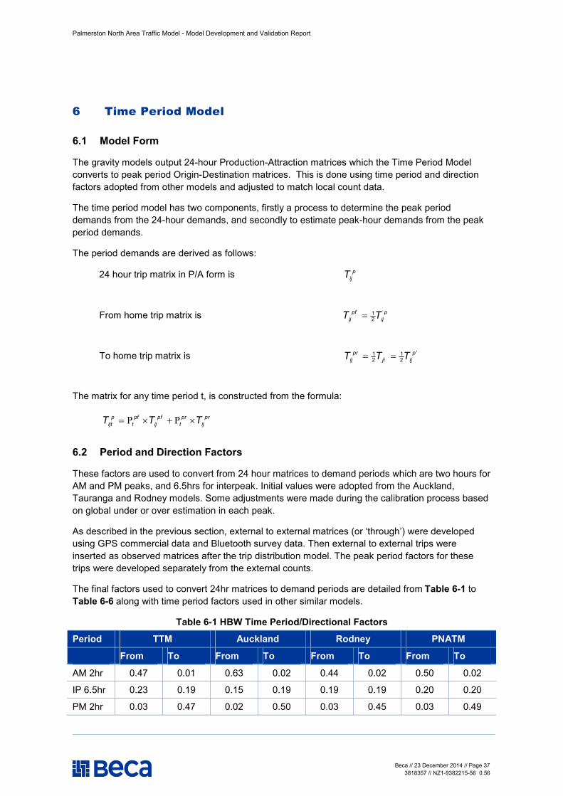
These factors are used to convert from 24 hour matrices to demand periods which are two hours for AM and PM peaks, and 6.5hrs for interpeak. Initial values were adopted from the Auckland, Tauranga and Rodney models. Some adjustments were made during the calibration process based on global under or over estimation in each peak.
As described in the previous section, external to external matrices (or ‘through’) were developed using GPS commercial data and Bluetooth survey data. Then external to external trips were inserted as observed matrices after the trip distribution model. The peak period factors for these trips were developed separately from the external counts.
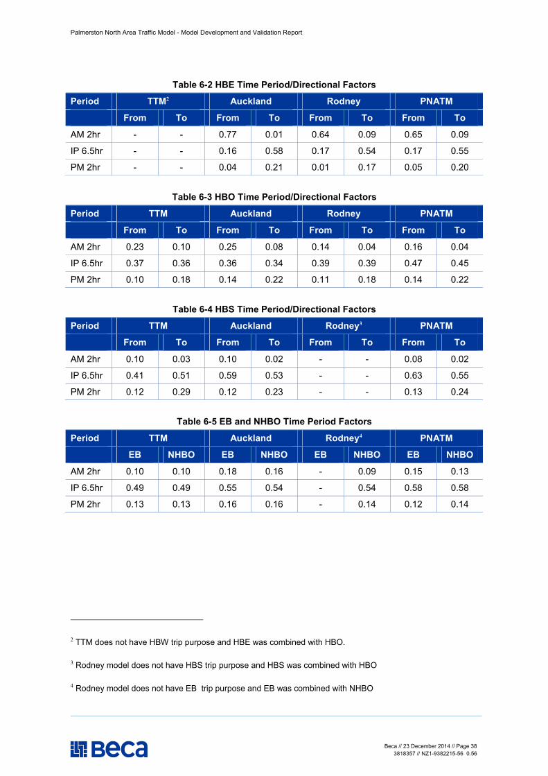
The final factors used to convert 24hr matrices to demand periods are detailed from Table 6-1 to Table 6-6 along with time period factors used in other similar models.
Table 6-1 HBW Time Period/Directional Factors
Period TTM Auckland Rodney PNATM
From To From To From To From To
AM 2hr 0.47 0.01 0.63 0.02 0.44 0.02 0.50 0.02
IP 6.5hr 0.23 0.19 0.15 0.19 0.19 0.19 0.20 0.20
PM 2hr 0.03 0.47 0.02 0.50 0.03 0.45 0.03 0.49
Palmerston North Area Traffic Model - Model Development and Validation Report
Beca // 23 December 2014 // Page 38 3818357 // NZ1-9382215-56 0.56
Table 6-2 HBE Time Period/Directional Factors
Period TTM2 Auckland Rodney PNATM
From To From To From To From To
AM 2hr - - 0.77 0.01 0.64 0.09 0.65 0.09
IP 6.5hr - - 0.16 0.58 0.17 0.54 0.17 0.55
PM 2hr - - 0.04 0.21 0.01 0.17 0.05 0.20
Table 6-3 HBO Time Period/Directional Factors
Period TTM Auckland Rodney PNATM
From To From To From To From To
AM 2hr 0.23 0.10 0.25 0.08 0.14 0.04 0.16 0.04
IP 6.5hr 0.37 0.36 0.36 0.34 0.39 0.39 0.47 0.45
PM 2hr 0.10 0.18 0.14 0.22 0.11 0.18 0.14 0.22
Table 6-4 HBS Time Period/Directional Factors
Period TTM Auckland Rodney3 PNATM
From To From To From To From To
AM 2hr 0.10 0.03 0.10 0.02 - - 0.08 0.02
IP 6.5hr 0.41 0.51 0.59 0.53 - - 0.63 0.55
PM 2hr 0.12 0.29 0.12 0.23 - - 0.13 0.24
Table 6-5 EB and NHBO Time Period Factors
Period TTM Auckland Rodney4 PNATM
EB NHBO EB NHBO EB NHBO EB NHBO
AM 2hr 0.10 0.10 0.18 0.16 - 0.09 0.15 0.13
IP 6.5hr 0.49 0.49 0.55 0.54 - 0.54 0.58 0.58
PM 2hr 0.13 0.13 0.16 0.16 - 0.14 0.12 0.14
2 TTM does not have HBW trip purpose and HBE was combined with HBO.
3 Rodney model does not have HBS trip purpose and HBS was combined with HBO
4 Rodney model does not have EB trip purpose and EB was combined with NHBO
Palmerston North Area Traffic Model - Model Development and Validation Report
Beca // 23 December 2014 // Page 39 3818357 // NZ1-9382215-56 0.56
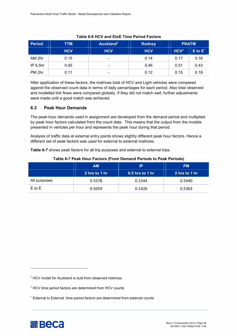
Table 6-6 HCV and EtoE Time Period Factors
Period TTM Auckland5 Rodney PNATM
HCV HCV HCV HCV6 E to E7
AM 2hr 0.15 - 0.14 0.17 0.16
IP 6.5hr 0.45 - 0.46 0.51 0.43
PM 2hr 0.11 - 0.12 0.15 0.18
After application of these factors, the matrices total of HCV and Light vehicles were compared against the observed count data in terms of daily percentages for each period. Also total observed and modelled link flows were compared globally. If they did not match well, further adjustments were made until a good match was achieved.
6.3 Peak Hour Demands
The peak-hour demands used in assignment are developed from the demand period and multiplied by peak hour factors calculated from the count data. This means that the output from the models presented in vehicles per hour and represents the peak hour during that period.
Analysis of traffic data at external entry points shows slightly different peak hour factors. Hence a different set of peak factors was used for external to external matrices.
Table 6-7 shows peak factors for all trip purposes and external to external trips.
Table 6-7 Peak Hour Factors (From Demand Periods to Peak Periods)
AM IP PM
2 hrs to 1 hr 6.5 hrs to 1 hr 2 hrs to 1 hr
All purposes 0.5578 0.1544 0.5440
E to E 0.5059 0.1426 0.5363
5 HCV model for Auckland is built from observed matrices.
6 HCV time period factors are determined from HCV counts
7 External to External time period factors are determined from external counts
Palmerston North Area Traffic Model - Model Development and Validation Report
Beca // 23 December 2014 // Page 40 3818357 // NZ1-9382215-56 0.56
7 Assignment Model
7.1 Model Form
Both assignment models in demand creation and final assignment module use two-class assignments for each period. Light and heavy vehicle matrices are assigned individually using differing path building parameters.
The assignment model applies the following iterative process:
n Least cost (All-or-Nothing) path building based on generalised cost; and n Capacity restraint using explicit junction delay modelling, speed-flow curves and volume-
averaging of flows.
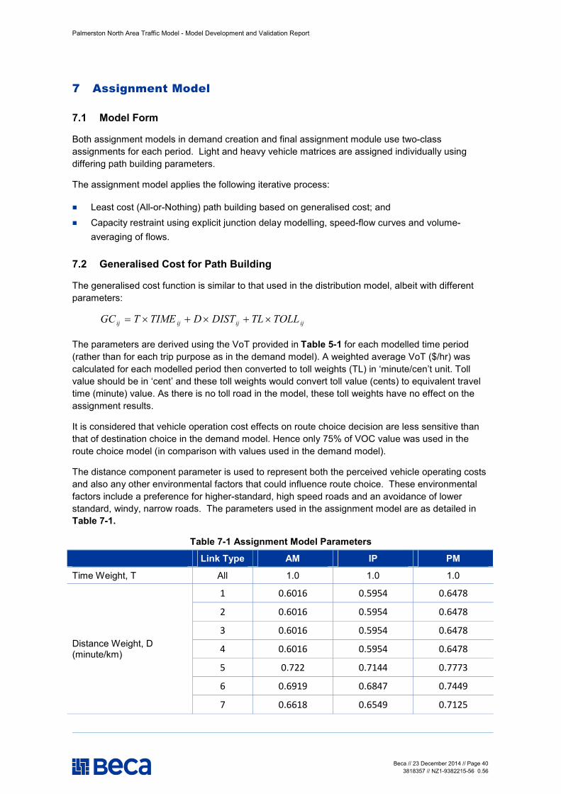
7.2 Generalised Cost for Path Building
The generalised cost function is similar to that used in the distribution model, albeit with different parameters:
ijijijij TOLLTLDISTDTIMETGC ×+×+×=
The parameters are derived using the VoT provided in Table 5-1 for each modelled time period (rather than for each trip purpose as in the demand model). A weighted average VoT ($/hr) was calculated for each modelled period then converted to toll weights (TL) in ‘minute/cen’t unit. Toll value should be in ‘cent’ and these toll weights would convert toll value (cents) to equivalent travel time (minute) value. As there is no toll road in the model, these toll weights have no effect on the assignment results.
It is considered that vehicle operation cost effects on route choice decision are less sensitive than that of destination choice in the demand model. Hence only 75% of VOC value was used in the route choice model (in comparison with values used in the demand model).
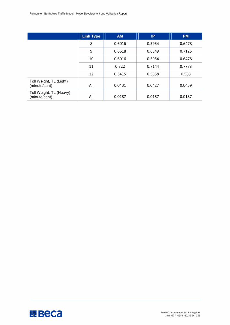
The distance component parameter is used to represent both the perceived vehicle operating costs and also any other environmental factors that could influence route choice. These environmental factors include a preference for higher-standard, high speed roads and an avoidance of lower standard, windy, narrow roads. The parameters used in the assignment model are as detailed in Table 7-1.
Table 7-1 Assignment Model Parameters
Link Type AM IP PM
Time Weight, T All 1.0 1.0 1.0
Distance Weight, D (minute/km)
1 0.6016 0.5954 0.6478
2 0.6016 0.5954 0.6478
3 0.6016 0.5954 0.6478
4 0.6016 0.5954 0.6478
5 0.722 0.7144 0.7773
6 0.6919 0.6847 0.7449
7 0.6618 0.6549 0.7125
Palmerston North Area Traffic Model - Model Development and Validation Report
Beca // 23 December 2014 // Page 41 3818357 // NZ1-9382215-56 0.56
Link Type AM IP PM
8 0.6016 0.5954 0.6478
9 0.6618 0.6549 0.7125
10 0.6016 0.5954 0.6478
11 0.722 0.7144 0.7773
12 0.5415 0.5358 0.583
Toll Weight, TL (Light) (minute/cent) All 0.0431 0.0427 0.0459
Toll Weight, TL (Heavy) (minute/cent) All 0.0187 0.0187 0.0187

Palmerston North Area Traffic Model - Model Development and Validation Report
Beca // 23 December 2014 // Page 42 3818357 // NZ1-9382215-56 0.56
8 Model Calibration and Validation Methodology
This chapter discusses the approach to model calibration/validation process.
The initial stage in this process was to undertake an independent internal review of model network coding, and demand inputs. This was undertaken by an experienced modeller independent from the project team. Input parameters were also shared with the peer reviewer, Tim Kelly.
In this context, model calibration is referred to as the process in which the network coding, delay parameters and demands were adjusted to match observed data. Validation is the process in which the resulting traffic flows, delays and speeds were compared to data not used in calibration.
8.1 Calibration Approach
The philosophy was to obtain satisfactory replication of base year (2013) conditions without excessive change to the demands. The main steps in the process were as follows:
n Start with the unmodified synthetic demands; n Calibrate the network speeds/assignment; n Make reasonable and realistic adjustments to the networks; n Check of the network and intersection coding where there are large delays; n Review of the locations of zone connectors and split of traffic (for multiple connectors) ; n Adjust the matrix using matrix estimation (this was minimal to start with); n Review network speed and assignment: n Make reasonable and realistic adjustments to the network; n Test different levels of matrix estimation; and n Review the effects of matrix estimation.
8.2 Key Validation Checks
The ‘fit’ of the model to observed data includes the following comparisons:
n Screenline vehicle flow totals by period and direction n Individual link vehicle flow totals by period and direction n HCV flows. Given the generally low proportion of HCV’s, these comparisons focus on daily
flows, however comparisons at peak period levels were also included n Turning flows at key junctions n Travel times on key routes

Palmerston North Area Traffic Model - Model Development and Validation Report
Beca // 23 December 2014 // Page 43 3818357 // NZ1-9382215-56 0.56
9 Matrix Estimation Process
The three stages of the modelling process, namely generation, distribution and assignment models are based on mathematical formulae. They produce synthetic trip matrices and assign traffic loadings to replicate complex human travel behaviour. Regarding trip generation, an average trip rate for each activity type has been used while there would be some variations in generation within the same activity type. Likewise distribution travel patterns are complex and vary between zones. Again, assignment models follow the least cost path and sometimes people do not necessarily travel on least cost routes. Studies suggest some 20% of route choices behaviours cannot be explained solely by minimum travel time and distance.
It has been recognised that such models are likely to have some discrepancies with observed data and would need some adjustments to the resulting trip tables to replicate observed conditions. The level of adjustment required is dependent on the required level of accuracy of the model and the quality of synthetic matrices. The General approach for the development of PNATM was to minimise the matrix adjustment while producing a high accuracy model to be fit for purpose for the studies of strategic and major urban area projects. Hence most of the efforts in model development were used to produce high quality synthetic matrices.
9.1 Light Vehicle Matrix Adjustment
The intention was to minimise the scale and effect of the final matrix adjustments. The matrix estimation process did not use all the count data, keeping a set of data independent for validation purposes. VOYAGER’s advanced matrix estimation process has been used which allows inclusion of trip-end data into the estimation (to lessen large-scale changes to zone totals) and the ability to estimate across screenline totals rather than just on individual links.
Before the matrix estimation process was undertaken, assignment (i.e. network) issues were identified and fixed to minimise undesired changes in matrices. This was undertaken in the interpeak model where unbalanced link flows are observed and issues could be identified. Also intersection coding was checked where large intersection delays were noticed.
After network issues were considered to be addressed, automated matrix estimation processes were used to adjust the peak period light matrices to observed data. This was done using the ANALYST component of the VOYAGER software which adjusts the trip tables to match screenline and link flows. To minimise the adjustments, the following measure have been undertaken:
n Synthetic matrix trip end totals were included in the estimation process with a higher confidence weight (compared to each cell in synthetic matrix) to minimise the changes in trip end totals.
n Screenline total was included where possible. Hence an estimation process targeted to match the total rather than individual link to avoid fixing assignment issues.
n Also a manual matrix adjustment process was introduced where changes in tripends were capped at +/-20%.
To understand the numbers of screenline and link counts required in the matrix estimation process, three levels of matrix estimation were undertaken.
n ME1: Screenline totals8 only (as shown in Figure 9-1) which are some 11% of total count data.
8 Only the total flow on a screenline is targeted, not the flow on individual links within that screenline.
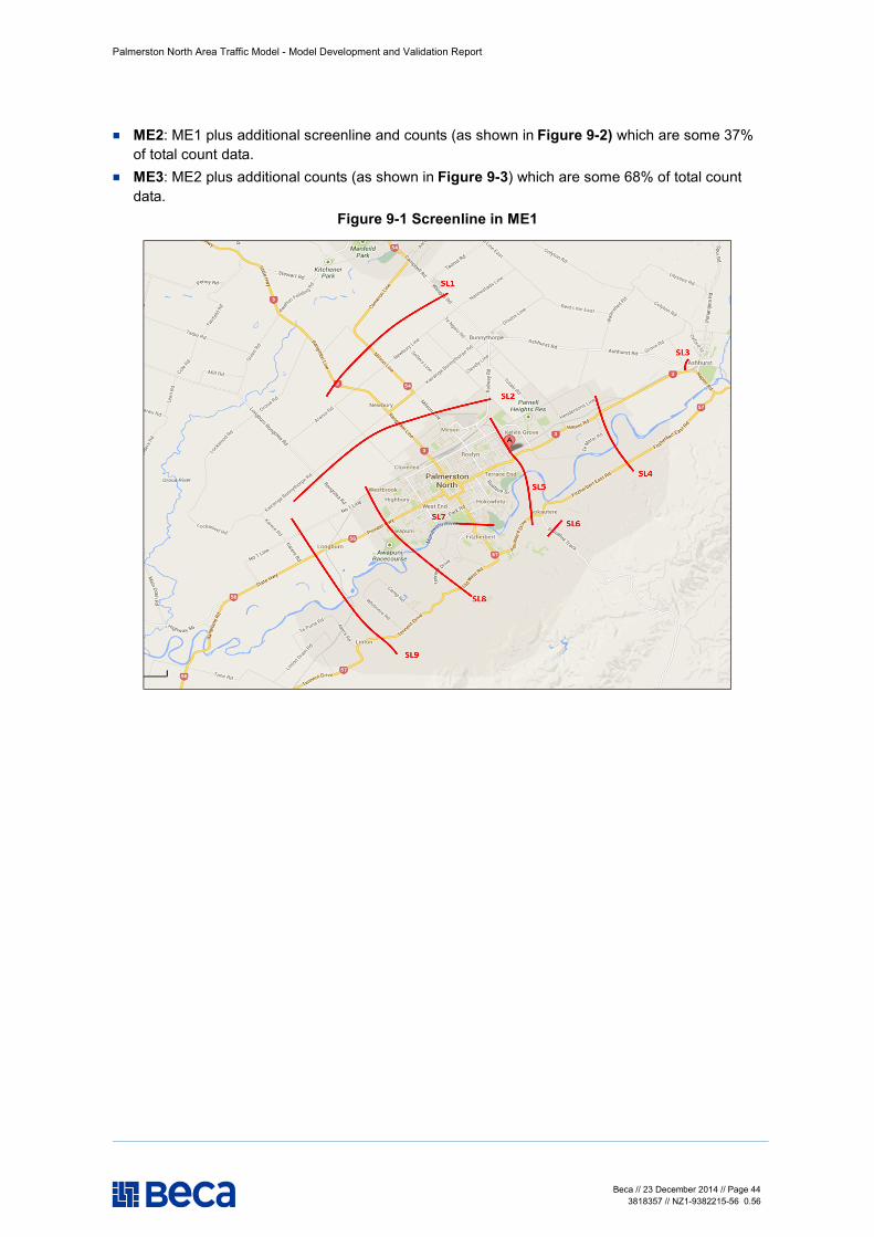
Palmerston North Area Traffic Model - Model Development and Validation Report
Beca // 23 December 2014 // Page 44 3818357 // NZ1-9382215-56 0.56
n ME2: ME1 plus additional screenline and counts (as shown in Figure 9-2) which are some 37% of total count data.
n ME3: ME2 plus additional counts (as shown in Figure 9-3) which are some 68% of total count data.
Figure 9-1 Screenline in ME1
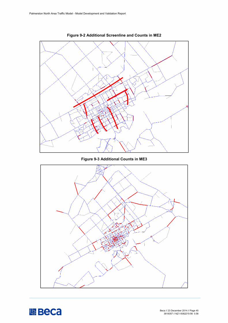
Palmerston North Area Traffic Model - Model Development and Validation Report
Beca // 23 December 2014 // Page 45 3818357 // NZ1-9382215-56 0.56
Figure 9-2 Additional Screenline and Counts in ME2
Figure 9-3 Additional Counts in ME3
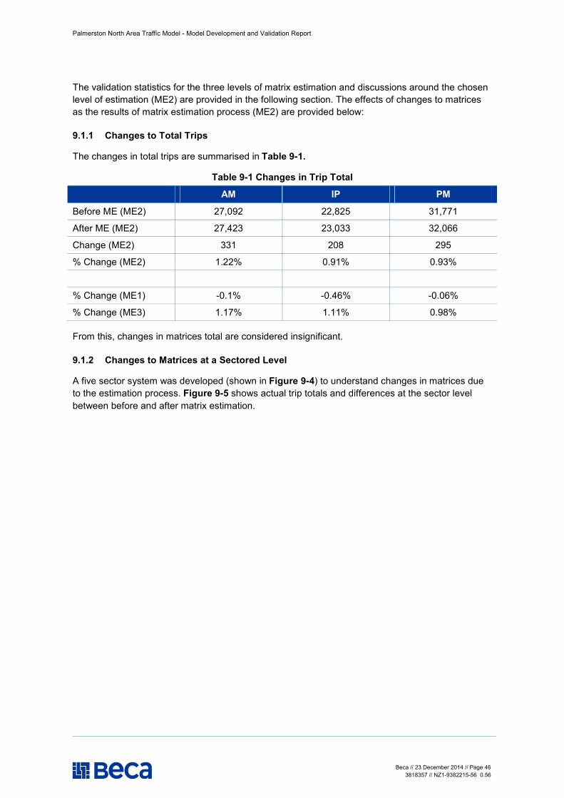
Palmerston North Area Traffic Model - Model Development and Validation Report
Beca // 23 December 2014 // Page 46 3818357 // NZ1-9382215-56 0.56
The validation statistics for the three levels of matrix estimation and discussions around the chosen level of estimation (ME2) are provided in the following section. The effects of changes to matrices as the results of matrix estimation process (ME2) are provided below:
9.1.1 Changes to Total Trips
The changes in total trips are summarised in Table 9-1.
Table 9-1 Changes in Trip Total
AM IP PM
Before ME (ME2) 27,092 22,825 31,771
After ME (ME2) 27,423 23,033 32,066
Change (ME2) 331 208 295
% Change (ME2) 1.22% 0.91% 0.93%
% Change (ME1) -0.1% -0.46% -0.06%
% Change (ME3) 1.17% 1.11% 0.98%
From this, changes in matrices total are considered insignificant.
9.1.2 Changes to Matrices at a Sectored Level
A five sector system was developed (shown in Figure 9-4) to understand changes in matrices due to the estimation process. Figure 9-5 shows actual trip totals and differences at the sector level between before and after matrix estimation.
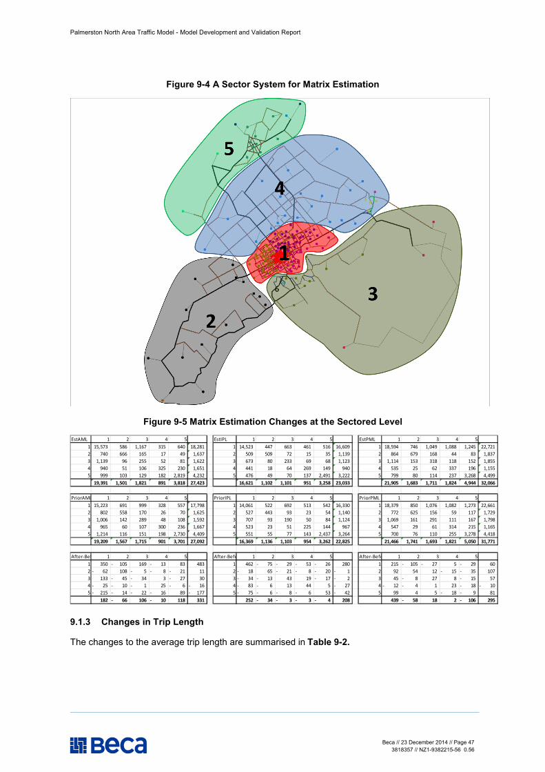
Palmerston North Area Traffic Model - Model Development and Validation Report
Beca // 23 December 2014 // Page 47 3818357 // NZ1-9382215-56 0.56
Figure 9-4 A Sector System for Matrix Estimation
Figure 9-5 Matrix Estimation Changes at the Sectored Level
EstAML 1 2 3 4 5 EstIPL 1 2 3 4 5 EstPML 1 2 3 4 51 15,573 586 1,167 315 640 18,281 1 14,523 447 663 461 516 16,609 1 18,594 746 1,049 1,088 1,245 22,721 2 740 666 165 17 49 1,637 2 509 509 72 15 35 1,139 2 864 679 168 44 83 1,837 3 1,139 96 255 52 81 1,622 3 673 80 233 69 68 1,123 3 1,114 153 318 118 152 1,855 4 940 51 106 325 230 1,651 4 441 18 64 269 149 940 4 535 25 62 337 196 1,155 5 999 103 129 182 2,819 4,232 5 476 49 70 137 2,491 3,222 5 799 80 114 237 3,268 4,499
19,391 1,501 1,821 891 3,818 27,423 16,621 1,102 1,101 951 3,258 23,033 21,905 1,683 1,711 1,824 4,944 32,066
PriorAML 1 2 3 4 5 PriorIPL 1 2 3 4 5 PriorPML 1 2 3 4 51 15,223 691 999 328 557 17,798 1 14,061 522 692 513 542 16,330 1 18,379 850 1,076 1,082 1,273 22,661 2 802 558 170 26 70 1,625 2 527 443 93 23 54 1,140 2 772 625 156 59 117 1,729 3 1,006 142 289 48 108 1,592 3 707 93 190 50 84 1,124 3 1,069 161 291 111 167 1,798 4 965 60 107 300 236 1,667 4 523 23 51 225 144 967 4 547 29 61 314 215 1,165 5 1,214 116 151 198 2,730 4,409 5 551 55 77 143 2,437 3,264 5 700 76 110 255 3,278 4,418
19,209 1,567 1,715 901 3,701 27,092 16,369 1,136 1,103 954 3,262 22,825 21,466 1,741 1,693 1,821 5,050 31,771
After-Before 1 2 3 4 5 After-Before 1 2 3 4 5 After-Before 1 2 3 4 51 350 105- 169 13- 83 483 1 462 75- 29- 53- 26- 280 1 215 105- 27- 5 29- 60 2 62- 108 5- 8- 21- 11 2 18- 65 21- 8- 20- 1- 2 92 54 12 15- 35- 107 3 133 45- 34- 3 27- 30 3 34- 13- 43 19 17- 2- 3 45 8- 27 8 15- 57 4 25- 10- 1- 25 6- 16- 4 83- 6- 13 44 5 27- 4 12- 4- 1 23 18- 10- 5 215- 14- 22- 16- 89 177- 5 75- 6- 8- 6- 53 42- 5 99 4 5 18- 9- 81
182 66- 106 10- 118 331 252 34- 3- 3- 4- 208 439 58- 18 2 106- 295
9.1.3 Changes in Trip Length
The changes to the average trip length are summarised in Table 9-2.
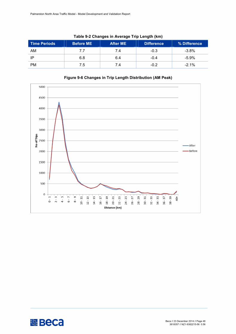
Palmerston North Area Traffic Model - Model Development and Validation Report
Beca // 23 December 2014 // Page 48 3818357 // NZ1-9382215-56 0.56
Table 9-2 Changes in Average Trip Length (km)
Time Periods Before ME After ME Difference % Difference
AM 7.7 7.4 -0.3 -3.8%
IP 6.8 6.4 -0.4 -5.9%
PM 7.5 7.4 -0.2 -2.1%
Figure 9-6 Changes in Trip Length Distribution (AM Peak)
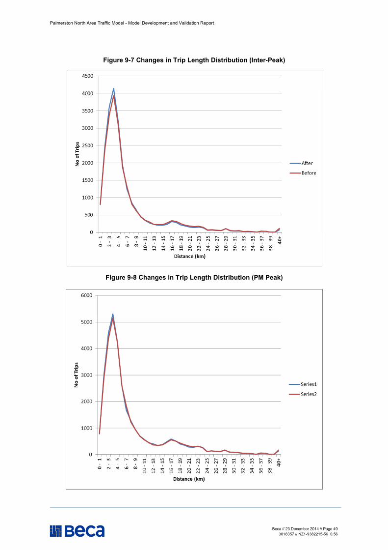
Palmerston North Area Traffic Model - Model Development and Validation Report
Beca // 23 December 2014 // Page 49 3818357 // NZ1-9382215-56 0.56
Figure 9-7 Changes in Trip Length Distribution (Inter-Peak)
Figure 9-8 Changes in Trip Length Distribution (PM Peak)
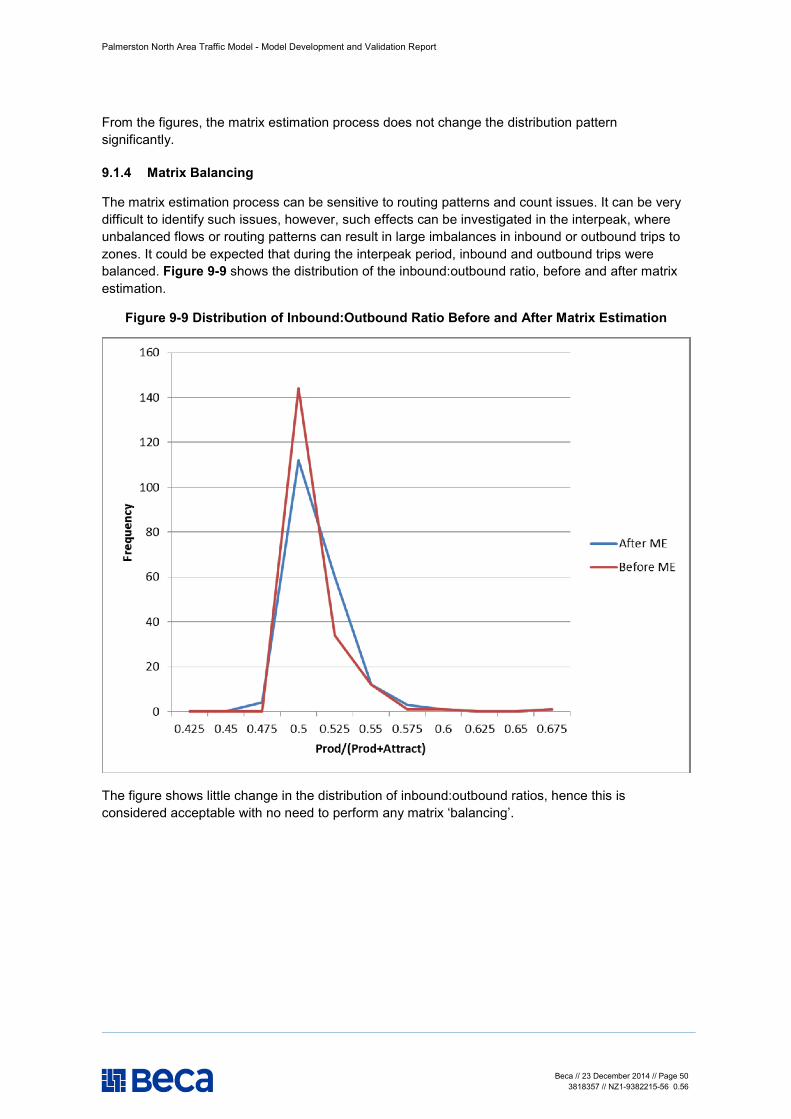
Palmerston North Area Traffic Model - Model Development and Validation Report
Beca // 23 December 2014 // Page 50 3818357 // NZ1-9382215-56 0.56
From the figures, the matrix estimation process does not change the distribution pattern significantly.
9.1.4 Matrix Balancing
The matrix estimation process can be sensitive to routing patterns and count issues. It can be very difficult to identify such issues, however, such effects can be investigated in the interpeak, where unbalanced flows or routing patterns can result in large imbalances in inbound or outbound trips to zones. It could be expected that during the interpeak period, inbound and outbound trips were balanced. Figure 9-9 shows the distribution of the inbound:outbound ratio, before and after matrix estimation.
Figure 9-9 Distribution of Inbound:Outbound Ratio Before and After Matrix Estimation
The figure shows little change in the distribution of inbound:outbound ratios, hence this is considered acceptable with no need to perform any matrix ‘balancing’.
Palmerston North Area Traffic Model - Model Development and Validation Report
Beca // 23 December 2014 // Page 51 3818357 // NZ1-9382215-56 0.56
9.2 Commercial Vehicle Matrix Development
A hybrid approach was used where both synthetic HCV matrix and commercial GPS data were utilised to generate the final HCV matrices. A matrix of daily truck movements was estimated from commercial GPS data. A synthetic model was also developed with trip rates and gravity model parameters calibrated to the observed matrix.
9.2.1 Commercial GPS Data
Due to recent advancements in technology, there is now significantly more data available regarding the movement of commercial vehicles around the network. Much of this is based on fleet GPS data which is able to track the movement of individual vehicles to a high level of accuracy. This data is able to be distilled into a table of trips which, in turn, can be converted into an origin-destination matrix. A data analytics application has been developed by Beca for the NZ Transport Agency (Teamview Clarity) that converts raw GPS data into trips tables and matrices for use in modelling. This was then modified to correlate to the zone system developed for Palmerston North.
The Teamview Clarity dataset, however, only includes a sample of the total commercial vehicle fleet (typically between 6% and 20%). Furthermore, the sample size is not consistent with some geographical areas better represented than others. In other words, it might be expected that close to 100% of all commercial vehicles may be captured for one meshblock (or model zone), whereas the sample size for an adjacent zone may be only 5% or 10%. Preliminary analysis of the dataset for the area around Palmerston North suggests a better than average sample size across the region, however local variability is still anticipated.
A trip definition model has been used in developing the HCV matrix. This assumes a trip features a minimum of 500m distanced travel and 2.5 minutes stop time at the end (this eliminates the effect of very short trips within yards and delays caused by traffic signals causing erroneous trips to be reported). External to external and external to internal (and reverse direction) trips are also included in the HCV matrix.
9.2.2 Synthetic HCV Matrix
Similar to other model’s trip purposes (e.g. HBW, HBS and etc...), HCV trip matrices were generated using trip rates and gravity parameters documented in the previous sections. These rates and parameters were adopted initially from the Tauranga model. These are further calibrated to local data (e.g. to match global daily HCV counts for the Palmerston North region). Also local adjustments have been undertaken (e.g. HCV trip rates for industrial type zones were increased as initial model runs show Tremaine Avenue has underestimation of HCV traffic).
9.2.3 A Hybrid Approach
Due to local variability or sampling issues of commercial GPS data, it was considered that the synthetic matrix would provide higher confidence in trip end totals. However, the GPS data would give a better distribution of HCV trips as it was based on the actual HCV movement data. From this, the following steps were taken to estimate the HCV matrix.
n Based on the analysis of commercial GPS and count data at the model external points, the sample rate is estimated to be some 20~25%.
n Hence the initial expansion factor of ‘4’ was applied to the Commercial GPS matrix. Then the matrix was loaded to the model.
n Initial matrix furnessing was undertaken for the Commercial GPS matrix to match the synthetic matrix’s trip ends. The purpose is to resolve the local variability sampling issue.
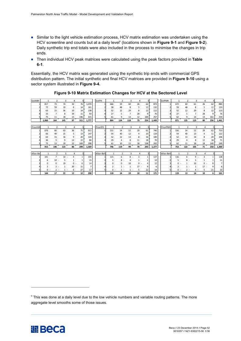
Palmerston North Area Traffic Model - Model Development and Validation Report
Beca // 23 December 2014 // Page 52 3818357 // NZ1-9382215-56 0.56
n Similar to the light vehicle estimation process, HCV matrix estimation was undertaken using the HCV screenline and counts but at a daily level9 (locations shown in Figure 9-1 and Figure 9-2). Daily synthetic trip end totals were also included in the process to minimise the changes in trip ends.
n Then individual HCV peak matrices were calculated using the peak factors provided in Table 6-1.
Essentially, the HCV matrix was generated using the synthetic trip ends with commercial GPS distribution pattern. The initial synthetic and final HCV matrices are provided in Figure 9-10 using a sector system illustrated in Figure 9-4.
Figure 9-10 Matrix Estimation Changes for HCV at the Sectored Level
EstAMH 1 2 3 4 5 EstIPH 1 2 3 4 5 EstPMH 1 2 3 4 51 817 73 74 32 76 1,070 1 666 59 60 26 62 873 1 672 60 61 26 62 880 2 72 59 10 6 14 161 2 58 48 8 5 12 132 2 59 48 8 5 12 133 3 63 15 36 10 14 138 3 52 12 29 8 12 112 3 52 12 29 8 12 113 4 33 7 8 34 11 93 4 27 5 7 28 9 76 4 27 5 7 28 9 76 5 75 11 18 15 196 315 5 61 9 14 12 160 257 5 62 9 14 13 161 259
1,060 164 145 97 311 1,777 864 134 118 79 254 1,449 871 135 119 80 256 1,461
PriorAMH 1 2 3 4 5 PriorIPH 1 2 3 4 5 PriorPMH 1 2 3 4 51 676 66 63 36 75 915 1 551 54 52 29 61 746 1 556 54 52 29 62 753 2 66 49 15 5 13 147 2 54 40 12 4 10 119 2 54 40 13 4 11 122 3 63 15 16 9 20 124 3 52 12 13 8 16 100 3 52 13 14 8 20 106 4 36 5 9 14 22 86 4 29 4 8 11 18 70 4 29 4 8 12 18 71 5 75 13 19 22 169 298 5 61 10 15 18 138 242 5 62 11 18 18 140 249
915 146 123 86 299 1,569 746 119 99 70 243 1,277 753 122 105 71 250 1,300
After-Before 1 2 3 4 5 After-Before 1 2 3 4 5 After-Before 1 2 3 4 51 141 7 10 4- 1 155 1 115 6 8 3- 1 127 1 116 6 9 3- 1 128 2 6 10 5- 1 1 15 2 5 8 4- 1 1 12 2 5 8 5- 1 1 11 3 0 0 19 0 6- 14 3 0 0 16 0 4- 12 3 0 1- 16 0 8- 7 4 2- 2 1- 20 11- 7 4 2- 1 1- 17 9- 6 4 2- 1 1- 17 9- 6 5 0- 2- 1- 6- 27 17 5 0- 1- 1- 5- 22 14 5 0- 2- 4- 5- 21 10
144 17 22 12 12 208 118 14 19 10 11 171 119 13 14 10 6 161
9 This was done at a daily level due to the low vehicle numbers and variable routing patterns. The more aggregate level smooths some of those issues.

Palmerston North Area Traffic Model - Model Development and Validation Report
Beca // 23 December 2014 // Page 53 3818357 // NZ1-9382215-56 0.56
10 Model Validation Results
This chapter discusses the results of the validation10 that has been undertaken.
10.1 Statistical Tests
The statistical tests and measurements to compare the model against observed data are based on common practice in NZ as well as appropriate guidelines such as the NZ Transport Agency’s Economic Evaluation Manual (EEM) and the draft guidelines produced by the NZ Modelling User Group (NZMUGS).
It should be noted that the NZMUGS criteria are in a draft state. Following this validation exercise, Beca suggested some changes to the criteria. This is likely to alter the criteria in the final release of the guidelines. Hence the NZMUGS criteria were used as a guide only to understand the level of model validation achieved.
10.1.1 Link Flow Comparison
The comparison of the modelled and the observed flows was undertaken using the following statistical tests:
n Actual and percentage difference between the modelled and the observed flows n RMSE (Root Mean Square Error). This is a global model test and the EEM suggests a target
value less than 30% n R2 (correlation co-efficient). This is also a global measure with EEM suggested targets of >0.85
in the wider model and >0.95 in the key study area. n GEH. This measure is calculated for each link and screenline. The EEM suggests the following
criteria for an acceptable fit of the model: – Individual links: § 60% with GEH<5 § 95% with GEH<10 § 100% with GEH<100
NZMUGS has different sets of criteria based on different types of the model category. The model categories comparable to the PNATM are:
n Category A – Regional n Category B - Strategic Network n Category C – Urban area n Category D – NZ Transport Agency Project
The definitions of these model categories are sourced from the NZMUGS Guideline as below:
“Model Type A: Regional Transport model (3, 4 or more Stage or Activity Based)
10 Some comparisons are against counts used in matrix estimation, which would be better described as calibration than validation. However for simplicity the terms are interchangeable here.
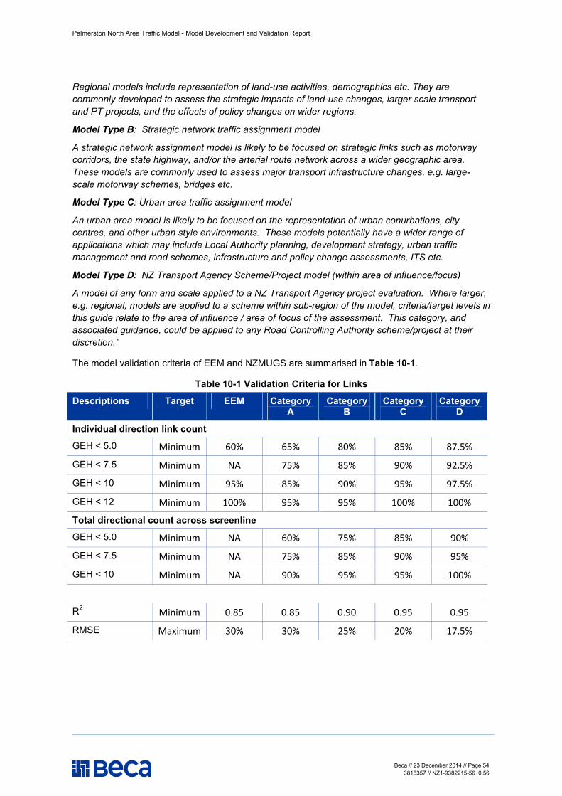
Palmerston North Area Traffic Model - Model Development and Validation Report
Beca // 23 December 2014 // Page 54 3818357 // NZ1-9382215-56 0.56
Regional models include representation of land-use activities, demographics etc. They are commonly developed to assess the strategic impacts of land-use changes, larger scale transport and PT projects, and the effects of policy changes on wider regions.
Model Type B: Strategic network traffic assignment model
A strategic network assignment model is likely to be focused on strategic links such as motorway corridors, the state highway, and/or the arterial route network across a wider geographic area. These models are commonly used to assess major transport infrastructure changes, e.g. large-scale motorway schemes, bridges etc.
Model Type C: Urban area traffic assignment model
An urban area model is likely to be focused on the representation of urban conurbations, city centres, and other urban style environments. These models potentially have a wider range of applications which may include Local Authority planning, development strategy, urban traffic management and road schemes, infrastructure and policy change assessments, ITS etc.
Model Type D: NZ Transport Agency Scheme/Project model (within area of influence/focus)
A model of any form and scale applied to a NZ Transport Agency project evaluation. Where larger, e.g. regional, models are applied to a scheme within sub-region of the model, criteria/target levels in this guide relate to the area of influence / area of focus of the assessment. This category, and associated guidance, could be applied to any Road Controlling Authority scheme/project at their discretion.”
The model validation criteria of EEM and NZMUGS are summarised in Table 10-1.
Table 10-1 Validation Criteria for Links
Descriptions Target EEM Category A
Category B
Category C
Category D
Individual direction link count
GEH < 5.0 Minimum 60% 65% 80% 85% 87.5%
GEH < 7.5 Minimum NA 75% 85% 90% 92.5%
GEH < 10 Minimum 95% 85% 90% 95% 97.5%
GEH < 12 Minimum 100% 95% 95% 100% 100%
Total directional count across screenline
GEH < 5.0 Minimum NA 60% 75% 85% 90%
GEH < 7.5 Minimum NA 75% 85% 90% 95%
GEH < 10 Minimum NA 90% 95% 95% 100%
R2 Minimum 0.85 0.85 0.90 0.95 0.95
RMSE Maximum 30% 30% 25% 20% 17.5%
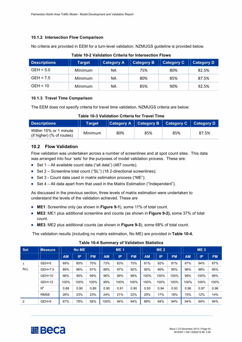
Palmerston North Area Traffic Model - Model Development and Validation Report
Beca // 23 December 2014 // Page 55 3818357 // NZ1-9382215-56 0.56
10.1.2 Intersection Flow Comparison
No criteria are provided in EEM for a turn-level validation. NZMUGS guideline is provided below.
Table 10-2 Validation Criteria for Intersection Flows
Descriptions Target Category A Category B Category C Category D
GEH < 5.0 Minimum NA 75% 80% 82.5%
GEH < 7.5 Minimum NA 80% 85% 87.5%
GEH < 10 Minimum NA 85% 90% 92.5%
10.1.3 Travel Time Comparison
The EEM does not specify criteria for travel time validation. NZMUGS criteria are below:
Table 10-3 Validation Criteria for Travel Time
Descriptions Target Category A Category B Category C Category D
Within 15% or 1 minute (if higher) (% of routes) Minimum 80% 85% 85% 87.5%
10.2 Flow Validation Flow validation was undertaken across a number of screenlines and at spot count sites. This data was arranged into four ‘sets’ for the purposes of model validation process. These are: n Set 1 – All available count data (“all data”) (487 counts); n Set 2 – Screenline total count (“SL”) (18 2-directional screenlines); n Set 3 - Count data used in matrix estimation process (“ME”); n Set 4 – All data apart from that used in the Matrix Estimation (“Independent”).
As discussed in the previous section, three levels of matrix estimation were undertaken to understand the levels of the validation achieved. These are
n ME1: Screenline only (as shown in Figure 9-1), some 11% of total count. n ME2: ME1 plus additional screenline and counts (as shown in Figure 9-2), some 37% of total
count. n ME3: ME2 plus additional counts (as shown in Figure 9-3), some 68% of total count.
The validation results (including no matrix estimation, No ME) are provided in Table 10-4.
Table 10-4 Summary of Validation Statistics Set Measure No ME ME 1 ME 2 ME 3
AM IP PM AM IP PM AM IP PM AM IP PM
1 ALL
GEH<5 69% 80% 70% 73% 83% 75% 81% 92% 81% 87% 94% 87%
GEH<7.5 89% 96% 91% 89% 97% 92% 95% 99% 95% 96% 98% 95%
GEH<10 96% 99% 99% 96% 99% 98% 100% 100% 100% 99% 100% 99%
GEH<12 100% 100% 100% 99% 100% 100% 100% 100% 100% 100% 100% 100%
R2 0.88 0.90 0.89 0.90 0.91 0.90 0.93 0.94 0.93 0.96 0.97 0.96
RMSE 26% 23% 23% 24% 21% 22% 20% 17% 18% 15% 12% 14%
2 GEH<5 67% 78% 56% 100% 94% 94% 89% 94% 94% 94% 94% 94%
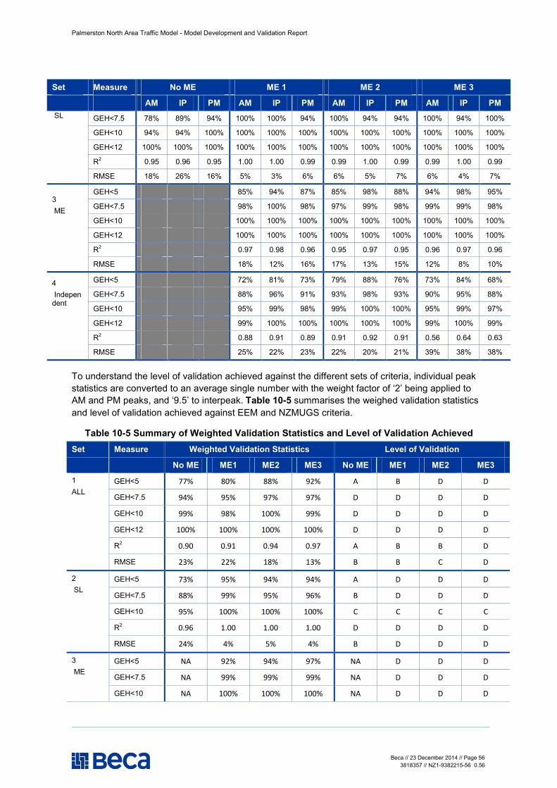
Palmerston North Area Traffic Model - Model Development and Validation Report
Beca // 23 December 2014 // Page 56 3818357 // NZ1-9382215-56 0.56
Set Measure No ME ME 1 ME 2 ME 3
AM IP PM AM IP PM AM IP PM AM IP PM SL
GEH<7.5 78% 89% 94% 100% 100% 94% 100% 94% 94% 100% 94% 100%
GEH<10 94% 94% 100% 100% 100% 100% 100% 100% 100% 100% 100% 100%
GEH<12 100% 100% 100% 100% 100% 100% 100% 100% 100% 100% 100% 100%
R2 0.95 0.96 0.95 1.00 1.00 0.99 0.99 1.00 0.99 0.99 1.00 0.99
RMSE 18% 26% 16% 5% 3% 6% 6% 5% 7% 6% 4% 7%
3 ME
GEH<5 85% 94% 87% 85% 98% 88% 94% 98% 95%
GEH<7.5 98% 100% 98% 97% 99% 98% 99% 99% 98%
GEH<10 100% 100% 100% 100% 100% 100% 100% 100% 100%
GEH<12 100% 100% 100% 100% 100% 100% 100% 100% 100%
R2 0.97 0.98 0.96 0.95 0.97 0.95 0.96 0.97 0.96
RMSE 18% 12% 16% 17% 13% 15% 12% 8% 10%
4 Independent
GEH<5 72% 81% 73% 79% 88% 76% 73% 84% 68%
GEH<7.5 88% 96% 91% 93% 98% 93% 90% 95% 88%
GEH<10 95% 99% 98% 99% 100% 100% 95% 99% 97%
GEH<12 99% 100% 100% 100% 100% 100% 99% 100% 99%
R2 0.88 0.91 0.89 0.91 0.92 0.91 0.56 0.64 0.63
RMSE 25% 22% 23% 22% 20% 21% 39% 38% 38%
To understand the level of validation achieved against the different sets of criteria, individual peak statistics are converted to an average single number with the weight factor of ‘2’ being applied to AM and PM peaks, and ‘9.5’ to interpeak. Table 10-5 summarises the weighed validation statistics and level of validation achieved against EEM and NZMUGS criteria.
Table 10-5 Summary of Weighted Validation Statistics and Level of Validation Achieved Set Measure Weighted Validation Statistics Level of Validation
No ME ME1 ME2 ME3 No ME ME1 ME2 ME3
1 ALL
GEH<5 77% 80% 88% 92% A B D D
GEH<7.5 94% 95% 97% 97% D D D D
GEH<10 99% 98% 100% 99% D D D D
GEH<12 100% 100% 100% 100% D D D D
R2 0.90 0.91 0.94 0.97 A B B D
RMSE 23% 22% 18% 13% B B C D
2 SL
GEH<5 73% 95% 94% 94% A D D D
GEH<7.5 88% 99% 95% 96% B D D D
GEH<10 95% 100% 100% 100% C C C C
R2 0.96 1.00 1.00 1.00 D D D D
RMSE 24% 4% 5% 4% B D D D
3 ME
GEH<5 NA 92% 94% 97% NA D D D
GEH<7.5 NA 99% 99% 99% NA D D D
GEH<10 NA 100% 100% 100% NA D D D
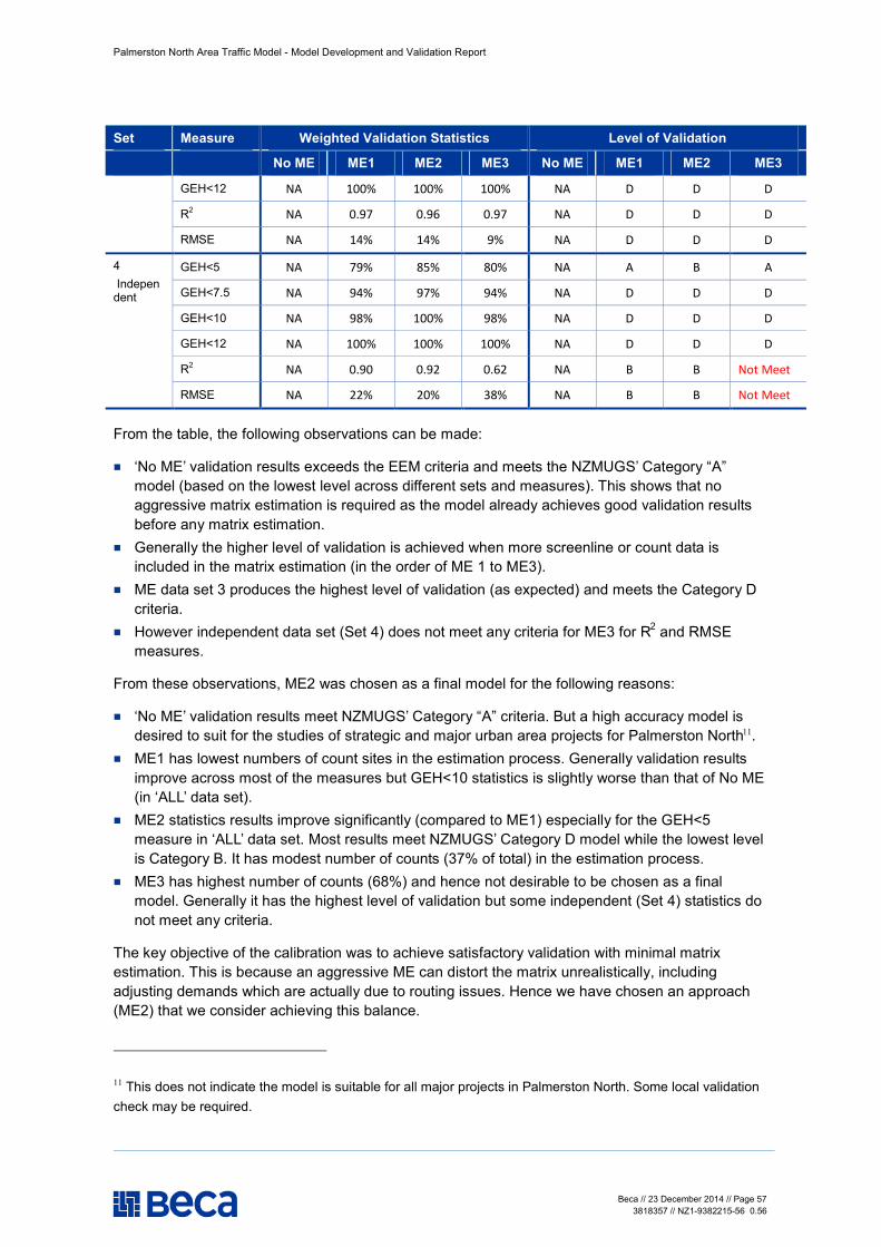
Palmerston North Area Traffic Model - Model Development and Validation Report
Beca // 23 December 2014 // Page 57 3818357 // NZ1-9382215-56 0.56
Set Measure Weighted Validation Statistics Level of Validation
No ME ME1 ME2 ME3 No ME ME1 ME2 ME3
GEH<12 NA 100% 100% 100% NA D D D
R2 NA 0.97 0.96 0.97 NA D D D
RMSE NA 14% 14% 9% NA D D D
4 Independent
GEH<5 NA 79% 85% 80% NA A B A
GEH<7.5 NA 94% 97% 94% NA D D D
GEH<10 NA 98% 100% 98% NA D D D
GEH<12 NA 100% 100% 100% NA D D D
R2 NA 0.90 0.92 0.62 NA B B Not Meet
RMSE NA 22% 20% 38% NA B B Not Meet
From the table, the following observations can be made:
n ‘No ME’ validation results exceeds the EEM criteria and meets the NZMUGS’ Category “A” model (based on the lowest level across different sets and measures). This shows that no aggressive matrix estimation is required as the model already achieves good validation results before any matrix estimation.
n Generally the higher level of validation is achieved when more screenline or count data is included in the matrix estimation (in the order of ME 1 to ME3).
n ME data set 3 produces the highest level of validation (as expected) and meets the Category D criteria.
n However independent data set (Set 4) does not meet any criteria for ME3 for R2 and RMSE measures.
From these observations, ME2 was chosen as a final model for the following reasons:
n ‘No ME’ validation results meet NZMUGS’ Category “A” criteria. But a high accuracy model is desired to suit for the studies of strategic and major urban area projects for Palmerston North11.
n ME1 has lowest numbers of count sites in the estimation process. Generally validation results improve across most of the measures but GEH<10 statistics is slightly worse than that of No ME (in ‘ALL’ data set).
n ME2 statistics results improve significantly (compared to ME1) especially for the GEH<5 measure in ‘ALL’ data set. Most results meet NZMUGS’ Category D model while the lowest level is Category B. It has modest number of counts (37% of total) in the estimation process.
n ME3 has highest number of counts (68%) and hence not desirable to be chosen as a final model. Generally it has the highest level of validation but some independent (Set 4) statistics do not meet any criteria.
The key objective of the calibration was to achieve satisfactory validation with minimal matrix estimation. This is because an aggressive ME can distort the matrix unrealistically, including adjusting demands which are actually due to routing issues. Hence we have chosen an approach (ME2) that we consider achieving this balance.
11 This does not indicate the model is suitable for all major projects in Palmerston North. Some local validation check may be required.
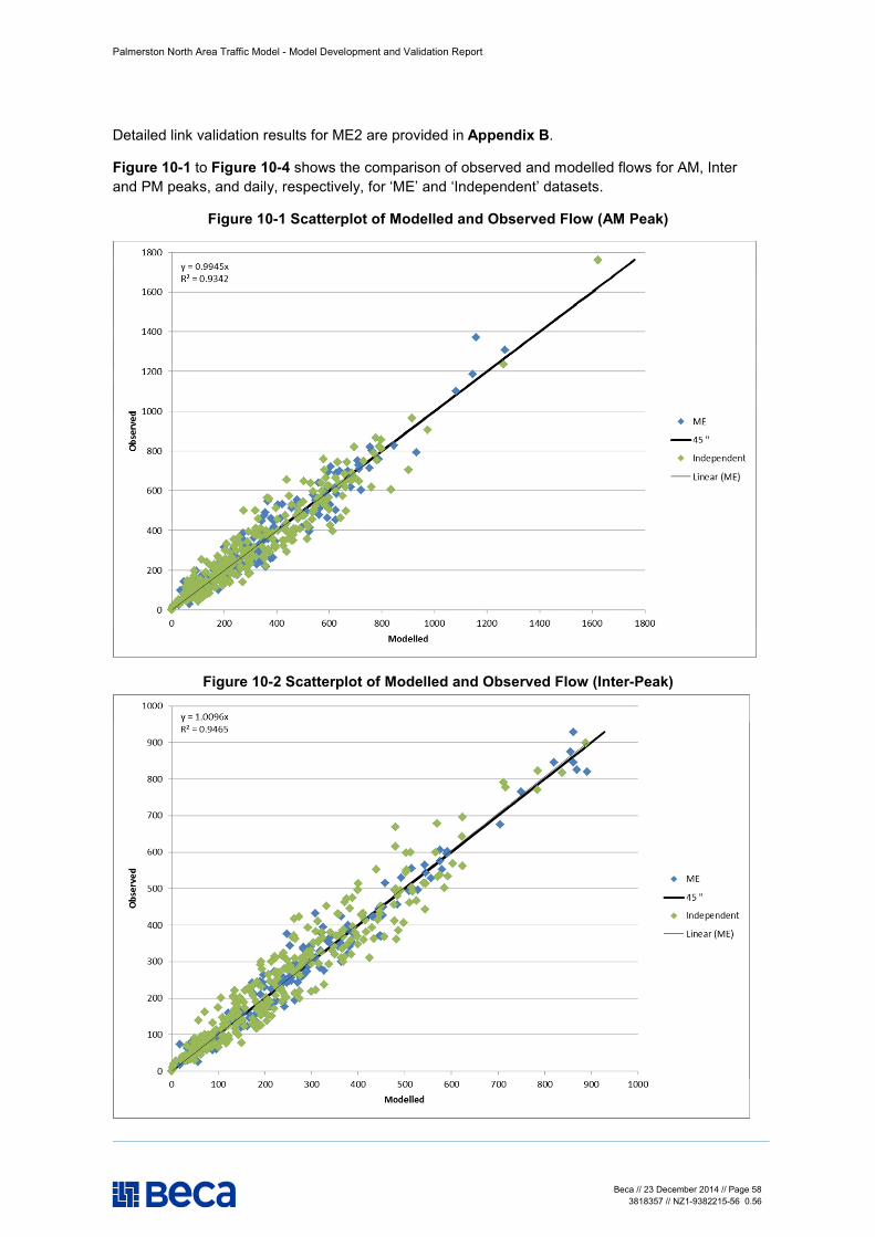
Palmerston North Area Traffic Model - Model Development and Validation Report
Beca // 23 December 2014 // Page 58 3818357 // NZ1-9382215-56 0.56
Detailed link validation results for ME2 are provided in Appendix B.
Figure 10-1 to Figure 10-4 shows the comparison of observed and modelled flows for AM, Inter and PM peaks, and daily, respectively, for ‘ME’ and ‘Independent’ datasets.
Figure 10-1 Scatterplot of Modelled and Observed Flow (AM Peak)
Figure 10-2 Scatterplot of Modelled and Observed Flow (Inter-Peak)
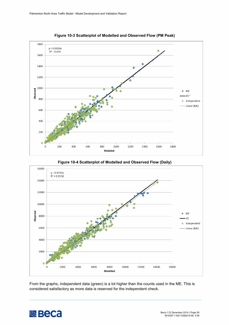
Palmerston North Area Traffic Model - Model Development and Validation Report
Beca // 23 December 2014 // Page 59 3818357 // NZ1-9382215-56 0.56
Figure 10-3 Scatterplot of Modelled and Observed Flow (PM Peak)
Figure 10-4 Scatterplot of Modelled and Observed Flow (Daily)
From the graphs, independent data (green) is a lot higher than the counts used in the ME. This is considered satisfactory as more data is reserved for the independent check.
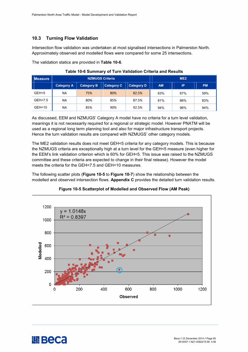
Palmerston North Area Traffic Model - Model Development and Validation Report
Beca // 23 December 2014 // Page 60 3818357 // NZ1-9382215-56 0.56
10.3 Turning Flow Validation
Intersection flow validation was undertaken at most signalised intersections in Palmerston North. Approximately observed and modelled flows were compared for some 25 intersections.
The validation statics are provided in Table 10-6.
Table 10-6 Summary of Turn Validation Criteria and Results Measure NZMUGS Criteria ME2
Category A Category B Category C Category D AM IP PM
GEH<5 NA 75% 80% 82.5% 63% 67% 59%
GEH<7.5 NA 80% 85% 87.5% 81% 86% 83%
GEH<10 NA 85% 90% 92.5% 94% 96% 94%
As discussed, EEM and NZMUGS’ Category A model have no criteria for a turn level validation, meanings it is not necessarily required for a regional or strategic model. However PNATM will be used as a regional long term planning tool and also for major infrastructure transport projects. Hence the turn validation results are compared with NZMUGS’ other category models.
The ME2 validation results does not meet GEH<5 criteria for any category models. This is because the NZMUGS criteria are exceptionally high at a turn level for the GEH<5 measure (even higher for the EEM’s link validation criterion which is 60% for GEH<5. This issue was raised to the NZMUGS committee and these criteria are expected to change in their final release). However the model meets the criteria for the GEH<7.5 and GEH<10 measures.
The following scatter plots (Figure 10-5 to Figure 10-7) show the relationship between the modelled and observed intersection flows. Appendix C provides the detailed turn validation results.
Figure 10-5 Scatterplot of Modelled and Observed Flow (AM Peak)
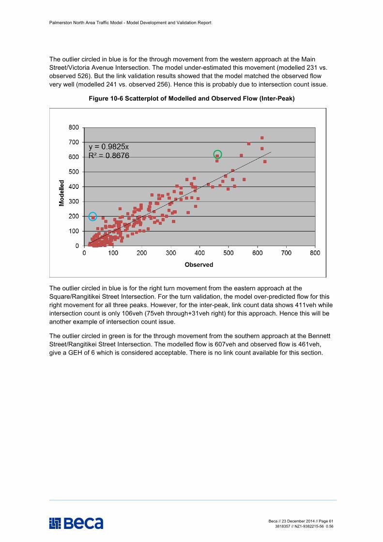
Palmerston North Area Traffic Model - Model Development and Validation Report
Beca // 23 December 2014 // Page 61 3818357 // NZ1-9382215-56 0.56
The outlier circled in blue is for the through movement from the western approach at the Main Street/Victoria Avenue Intersection. The model under-estimated this movement (modelled 231 vs. observed 526). But the link validation results showed that the model matched the observed flow very well (modelled 241 vs. observed 256). Hence this is probably due to intersection count issue.
Figure 10-6 Scatterplot of Modelled and Observed Flow (Inter-Peak)
The outlier circled in blue is for the right turn movement from the eastern approach at the Square/Rangitikei Street Intersection. For the turn validation, the model over-predicted flow for this right movement for all three peaks. However, for the inter-peak, link count data shows 411veh while intersection count is only 106veh (75veh through+31veh right) for this approach. Hence this will be another example of intersection count issue.
The outlier circled in green is for the through movement from the southern approach at the Bennett Street/Rangitikei Street Intersection. The modelled flow is 607veh and observed flow is 461veh, give a GEH of 6 which is considered acceptable. There is no link count available for this section.
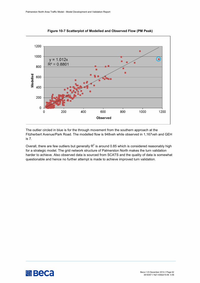
Palmerston North Area Traffic Model - Model Development and Validation Report
Beca // 23 December 2014 // Page 62 3818357 // NZ1-9382215-56 0.56
Figure 10-7 Scatterplot of Modelled and Observed Flow (PM Peak)
The outlier circled in blue is for the through movement from the southern approach at the Fitzherbert Avenue/Park Road. The modelled flow is 948veh while observed in 1,167veh and GEH is 7.
Overall, there are few outliers but generally R2 is around 0.85 which is considered reasonably high for a strategic model. The grid network structure of Palmerston North makes the turn validation harder to achieve. Also observed data is sourced from SCATS and the quality of data is somewhat questionable and hence no further attempt is made to achieve improved turn validation.
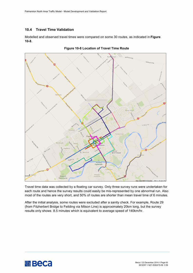
Palmerston North Area Traffic Model - Model Development and Validation Report
Beca // 23 December 2014 // Page 63 3818357 // NZ1-9382215-56 0.56
10.4 Travel Time Validation
Modelled and observed travel times were compared on some 30 routes, as indicated in Figure 10-8.
Figure 10-8 Location of Travel Time Route
Travel time data was collected by a floating car survey. Only three survey runs were undertaken for each route and hence the survey results could easily be mis-represented by one abnormal run. Also most of the routes are very short, and 50% of routes are shorter than mean travel time of 6 minutes.
After the initial analysis, some routes were excluded after a sanity check. For example, Route 29 (from Fitzherbert Bridge to Feilding via Milson Line) is approximately 20km long, but the survey results only shows 8.5 minutes which is equivalent to average speed of 140km/hr.
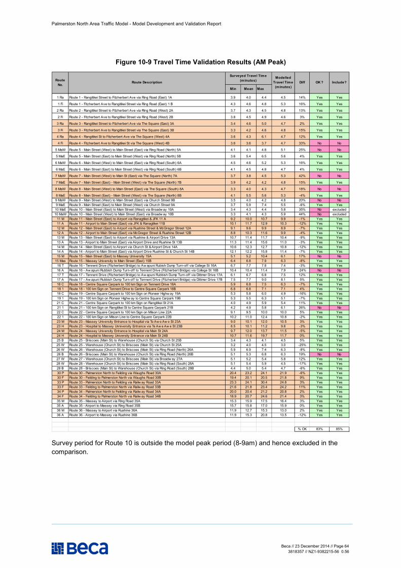
Palmerston North Area Traffic Model - Model Development and Validation Report
Beca // 23 December 2014 // Page 64 3818357 // NZ1-9382215-56 0.56
Figure 10-9 Travel Time Validation Results (AM Peak)
Surveyed Travel Time (minutes)
Min Mean Max
1 Ra Route 1 - Rangitikei Street to Fitzherbert Ave via Ring Road (East) 1A 3.9 4.0 4.4 4.5 14% Yes Yes
1 Fi Route 1 - Fitzherbert Ave to Rangitikei Street via Ring Road (East) 1 B 4.3 4.6 4.8 5.3 16% Yes Yes
2 Ra Route 2 - Rangitikei Street to Fitzherbert Ave via Ring Road (West) 2A 3.7 4.3 4.5 4.8 13% Yes Yes
2 Fi Route 2 - Fitzherbert Ave to Rangitikei Street via Ring Road (West) 2B 3.8 4.5 4.9 4.6 3% Yes Yes
3 Ra Route 3 - Rangitikei Street to Fitzherbert Ave via The Square (East) 3A 3.4 4.6 5.0 4.7 2% Yes Yes
3 Fi Route 3 - Fitzherbert Ave to Rangitikei Street via The Square (East) 3B 3.3 4.2 4.6 4.8 15% Yes Yes
4 Ra Route 4 - Rangitikei St to Fitzherbert Ave via The Square (West) 4A 3.6 4.3 6.1 4.7 12% Yes Yes
4 Fi Route 4 - Fitzherbert Ave to Rangitikei St via The Square (West) 4B 3.6 3.6 3.7 4.7 33% No No
5 MaW Route 5 - Main Street (West) to Main Street (East) via Ring Road (North) 5A 4.1 4.1 4.8 5.1 25% No No
5 MaE Route 5 - Main Street (East) to Main Street (West) via Ring Road (North) 5B 3.6 5.4 6.5 5.6 4% Yes Yes
6 MaW Route 6 - Main Street (West) to Main Street (East) via Ring Road (South) 6A 4.5 4.6 5.2 5.3 16% Yes Yes
6 MaE Route 6 - Main Street (East) to Main Street (West) via Ring Road (South) 6B 4.1 4.5 4.8 4.7 4% Yes Yes
7 MaW Route 7 - Main Street (West) to Main St (East) via The Square (North) 7A 3.7 3.8 4.5 5.3 42% No No
7 MaE Route 7 - Main Street (East) - Main Street (West) via The Square (North) 7B 3.9 4.2 4.2 4.8 15% Yes Yes
8 MaW Route 8 - Main Street (West) to Main Street (East) via The Square (South) 8A 3.3 4.0 4.3 4.7 18% No No
8 MaE Route 8 - Main Street (East) - Main Street (West) via The Square (North) 8B 4.1 5.5 5.6 5.3 -4% Yes Yes9 MaW Route 9 - Main Street (West) to Main Street (East) via Church Street 9B 3.5 4.0 4.2 4.8 20% No No9 MaE Route 9 - Main Street (East) to Main Street (West) via Church Street 9A 3.7 5.9 7.4 5.5 -6% Yes Yes
10 MaE Route 10 - Main Street (East) to Main Street (West) via Broadw ay 10A 3.4 4.3 4.4 5.8 35% No excluded10 MaW Route 10 - Main Street (West) to Main Street (East) via Broadw ay 10B 3.3 4.1 4.3 5.9 44% No excluded
11 M Route 11 - Main Street (East) to Airport via Ranagtikei & JFK 11 A 9.2 10.0 10.7 9.9 -1% Yes Yes11 A Route 11 - Airport to Main Street (East) via JFK & Ranagtikei 11B 10.1 11.7 12.9 10.3 -12% Yes Yes12 M Route 12 - Main Street (East) to Airport via Ruahine Street & McGregor Street 12A 9.1 9.6 9.9 8.9 -7% Yes Yes12 A Route 12 - Airport to Main Street (East) via McGregor Street & Ruahine Street 12B 8.8 10.3 11.6 9.9 -4% Yes Yes13 M Route 13 - Main Street (East) to Airport via Ruahine & Airport Drive 13A 10.7 11.4 11.7 10.4 -9% Yes Yes13 A Route 13 - Airport to Main Street (East) via Airport Drive and Ruahine St 13B 11.3 11.4 15.6 11.0 -3% Yes Yes14 M Route 14 - Main Street (East) to Airport via Church St & Airport Drive 14A 10.6 12.3 12.7 10.8 -12% Yes Yes14 A Route 14 - Airport to Main Street (East) via Airport Drive Ruahine St & Church St 14B 12.1 12.2 15.8 11.4 -7% Yes Yes15 M Route 15 - Main Street (East) to Massey University 15A 5.1 5.2 10.4 6.1 17% No No
15 Mas Route 15 - Massey University to Main Street (East) 15B 6.4 6.8 7.9 6.3 -8% Yes Yes16 T Route 16 - Tennent Drive (Fitzherbert Bridge) to Aw apuni Rubish Dump Turn-off via College St 16A 6.7 7.7 7.8 7.4 -3% Yes Yes16 A Route 16 - Aw apuni Rubbish Dump Turn-off to Tennent Drive (Fitzherbert Bridge) via College St 16B 10.4 10.4 11.4 7.9 -24% No No17 T Route 17 - Tennent Drive (Fitzherbert Bridge) to Aw apuni Rubbish Dump Turn-off via Dittmer Drive 17A 6.1 6.7 6.8 7.5 12% Yes Yes17 A Route 17 - Aw apuni Rubbish Dump Turn-off to Tennent Drive (Fitzherbert Bridge) via Dittmer Drive 17B 7.5 7.7 9.0 8.1 5% Yes Yes18 C Route 18 - Centre Square Carpark to 100 km Sign on Tennent Drive 18A 5.9 6.8 7.5 6.3 -7% Yes Yes18 1 Route 18 - 100 km Sign on Tennent Drive to Centre Square Carpark 18B 6.8 6.8 7.1 7.1 4% Yes Yes19 C Route 19 - Centre Square Carpark to 100 km Sign on Pioneer Highw ay 19A 5.3 5.8 6.0 4.9 -16% Yes Yes19 1 Route 19 - 100 km Sign on Pioneer Highw ay to Centre Square Carpark 19B 5.3 5.5 6.3 5.1 -7% Yes Yes21 C Route 21 - Centre Square Carpark to 100 km Sign on Rangitikei St 21A 4.0 4.9 5.9 5.4 11% Yes Yes21 1 Route 21 - 100 km Sign on Rangitikei St to Centre Square Carpark 21B 4.2 4.9 5.8 6.1 26% No No22 C Route 22 - Centre Square Carpark to 100 km Sign on Milson Line 22A 9.1 9.5 10.0 10.0 5% Yes Yes22 1 Route 22 - 100 km Sign on Milson Line to Centre Square Carpark 22B 10.2 11.0 12.4 10.8 -2% Yes Yes23 M Route 23 - Massey University Entrance to Hospital via Te Aw e Aw e St 23A 9.0 10.1 12.0 10.5 3% Yes Yes23 H Route 23 - Hospital to Massey Unniversity Entrance via Te Aw e Aw e St 23B 8.5 10.1 11.2 9.8 -3% Yes Yes24 M Route 24 - Massey University Entrance to Hospital via Main St 24A 9.7 12.0 13.7 11.5 -5% Yes Yes24 H Route 24 - Hospital to Massey University Entrance via Main St 24B 10.7 11.6 19.7 11.7 0% Yes Yes25 B Route 25 - Briscoes (Main St) to Warehouse (Church St) via Church St 25B 3.4 4.3 4.1 4.5 5% Yes Yes25 W Route 25 - Warehouse (Church St) to Briscoes (Main St) via Church St 25A 3.2 4.0 4.5 3.0 -25% Yes Yes26 W Route 26 - Warehouse (Church St) to Briscoes (Main St) via Ring Road (North) 26A 5.9 6.9 7.4 6.3 -8% Yes Yes26 B Route 26 - Briscoes (Main St) to Warehouse (Church St) via Ring Road (North) 26B 5.1 5.3 6.8 6.3 19% No No27 W Route 27 - Warehouse (Church St) to Briscoes (Main St) via Broadw ay 27A 5.1 5.2 5.4 5.8 12% Yes Yes28 W Route 28 - Warehouse (Church St) to Briscoes (Main St) via Ring Road (South) 28A 5.1 5.4 5.9 4.5 -17% Yes Yes28 B Route 28 - Briscoes (Main St) to Warehouse (Church St) via Ring Road (South) 28B 4.4 5.0 5.4 4.7 -6% Yes Yes30 P Route 30 - Palmerston North to Feilding via Waughs Road 30A 20.4 23.2 24.1 21.9 -6% Yes Yes30 F Route 30 - Feilding to Palmerston North via Waughs Road 30B 19.4 20.1 20.5 21.8 9% Yes Yes33 P Route 33 - Palmerston North to Feilding via Railw ay Road 33A 23.3 24.1 30.4 24.8 3% Yes Yes33 F Route 33 - Feilding to Palmerston North via Railw ay Road 33B 21.6 21.8 23.4 24.2 11% Yes Yes34 P Route 34 - Palmerston North to Feilding via Railw ay Road 34A 20.0 20.4 21.2 20.8 2% Yes Yes34 F Route 34 - Feilding to Palmerston North via Railw ay Road 34B 18.9 20.7 24.6 21.4 3% Yes Yes35 M Route 35 - Massey to Airport via Ring Road 35A 15.3 15.9 17.5 16.4 3% Yes Yes35 A Route 35 - Airport to Massey via Ring Road 35B 15.7 15.8 17.0 15.9 0% Yes Yes36 M Route 36 - Massey to Airport via Ruahine 36A 11.9 12.7 15.3 13.0 2% Yes Yes36 A Route 36 - Airport to Massey via Ruahine 36B 11.9 15.3 20.8 13.5 -12% Yes Yes
% OK 83% 85%
Include?OK ?DiffModelled
Travel Time (minutes)
Route No.
Route Description
Survey period for Route 10 is outside the model peak period (8-9am) and hence excluded in the comparison.
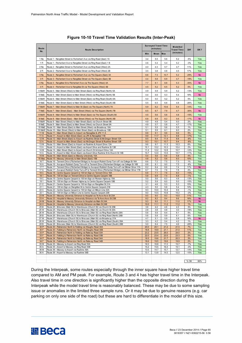
Palmerston North Area Traffic Model - Model Development and Validation Report
Beca // 23 December 2014 // Page 65 3818357 // NZ1-9382215-56 0.56
Figure 10-10 Travel Time Validation Results (Inter-Peak)
Surveyed Travel Time (m inutes)
Min Mean Max
1 Ra Route 1 - Rangitikei Street to Fitzherbert Ave via Ring Road (East) 1A 3.4 5.5 5.6 5.2 -5% Yes
1 Fi Route 1 - Fitzherbert Ave to Rangitikei Street via Ring Road (East) 1 B 4.6 5.4 5.4 5.2 -3% Yes
2 Ra Route 2 - Rangitikei Street to Fitzherbert Ave via Ring Road (West) 2A 4.0 4.3 5.7 4.7 11% Yes
2 Fi Route 2 - Fitzherbert Ave to Rangitikei Street via Ring Road (West) 2B 3.5 3.8 4.8 4.5 17% Yes
3 Ra Route 3 - Rangitikei Street to Fitzherbert Ave via The Square (East) 3A 6.6 7.3 10.7 5.2 -29% No
3 Fi Route 3 - Fitzherbert Ave to Rangitikei Street via The Square (East) 3B 4.4 5.8 6.9 4.7 -19% Yes
4 Ra Route 4 - Rangitikei St to Fitzherbert Ave via The Square (West) 4A 7.7 8.1 8.8 5.3 -35% No
4 Fi Route 4 - Fitzherbert Ave to Rangitikei St via The Square (West) 4B 4.5 5.2 6.5 5.2 0% Yes
5 MaW Route 5 - Main Street (West) to Main Street (East) via Ring Road (North) 5A 4.9 5.9 5.9 5.2 -13% Yes
5 MaE Route 5 - Main Street (East) to Main Street (West) via Ring Road (North) 5B 4.4 4.6 5.3 5.4 18% No
6 MaW Route 6 - Main Street (West) to Main Street (East) via Ring Road (South) 6A 5.0 5.0 5.2 5.2 5% Yes
6 MaE Route 6 - Main Street (East) to Main Street (West) via Ring Road (South) 6B 5.5 6.5 6.8 4.8 -26% Yes
7 MaW Route 7 - Main Street (West) to Main St (East) via The Square (North) 7A 5.9 6.2 10.6 5.4 -14% Yes
7 MaE Route 7 - Main Street (East) - Main Street (West) via The Square (North) 7B 6.5 6.7 7.9 4.7 -30% No
8 MaW Route 8 - Main Street (West) to Main Street (East) via The Square (South) 8A 4.5 5.6 5.8 4.8 -15% Yes
8 MaE Route 8 - Main Street (East) - Main Street (West) via The Square (North) 8B 6.8 6.8 8.2 5.6 -17% No9 MaW Route 9 - Main Street (West) to Main Street (East) via Church Street 9B 4.9 4.9 5.4 5.0 2% Yes9 MaE Route 9 - Main Street (East) to Main Street (West) via Church Street 9A 4.9 5.7 5.8 4.7 -17% Yes10 MaE Route 10 - Main Street (East) to Main Street (West) via Broadw ay 10A 5.1 5.5 5.6 5.5 1% Yes10 MaW Route 10 - Main Street (West) to Main Street (East) via Broadw ay 10B 5.1 5.9 6.1 6.0 2% Yes
11 M Route 11 - Main Street (East) to Airport via Ranagtikei & JFK 11 A 8.8 9.1 9.6 9.6 5% Yes11 A Route 11 - Airport to Main Street (East) via JFK & Ranagtikei 11B 9.9 11.7 12.1 9.8 -17% Yes12 M Route 12 - Main Street (East) to Airport via Ruahine Street & McGregor Street 12A 8.5 9.4 11.4 8.8 -6% Yes12 A Route 12 - Airport to Main Street (East) via McGregor Street & Ruahine Street 12B 9.3 10.1 10.7 9.4 -8% Yes13 M Route 13 - Main Street (East) to Airport via Ruahine & Airport Drive 13A 9.6 9.7 11.3 10.3 6% Yes13 A Route 13 - Airport to Main Street (East) via Airport Drive and Ruahine St 13B 10.1 10.2 10.3 10.4 2% Yes14 M Route 14 - Main Street (East) to Airport via Church St & Airport Drive 14A 11.4 12.2 12.8 10.7 -12% Yes14 A Route 14 - Airport to Main Street (East) via Airport Drive Ruahine St & Church St 14B 10.7 12.0 13.5 10.7 -11% Yes15 M Route 15 - Main Street (East) to Massey University 15A 5.4 5.6 6.6 5.8 4% Yes
15 Mas Route 15 - Massey University to Main Street (East) 15B 4.8 5.2 5.6 6.0 15% Yes16 T Route 16 - Tennent Drive (Fitzherbert Bridge) to Aw apuni Rubish Dump Turn-off via College St 16A 6.6 7.2 7.5 7.3 1% Yes16 A Route 16 - Aw apuni Rubbish Dump Turn-off to Tennent Drive (Fitzherbert Bridge) via College St 16B 6.8 8.1 9.0 7.5 -8% Yes17 T Route 17 - Tennent Drive (Fitzherbert Bridge) to Aw apuni Rubbish Dump Turn-off via Dittmer Drive 17A 6.2 6.4 6.6 7.4 17% No17 A Route 17 - Aw apuni Rubbish Dump Turn-off to Tennent Drive (Fitzherbert Bridge) via Dittmer Drive 17B 6.7 7.5 7.6 7.8 4% Yes18 C Route 18 - Centre Square Carpark to 100 km Sign on Tennent Drive 18A 6.8 7.1 7.6 6.0 -15% Yes18 1 Route 18 - 100 km Sign on Tennent Drive to Centre Square Carpark 18B 5.8 6.9 7.4 6.8 -1% Yes19 C Route 19 - Centre Square Carpark to 100 km Sign on Pioneer Highw ay 19A 5.0 5.6 6.3 4.9 -13% Yes19 1 Route 19 - 100 km Sign on Pioneer Highw ay to Centre Square Carpark 19B 5.2 5.9 6.0 5.0 -15% Yes21 C Route 21 - Centre Square Carpark to 100 km Sign on Rangitikei St 21A 3.1 4.6 5.3 5.3 15% Yes21 1 Route 21 - 100 km Sign on Rangitikei St to Centre Square Carpark 21B 4.3 5.0 5.8 5.4 10% Yes22 C Route 22 - Centre Square Carpark to 100 km Sign on Milson Line 22A 9.3 10.0 10.4 9.9 -1% Yes22 1 Route 22 - 100 km Sign on Milson Line to Centre Square Carpark 22B 9.0 10.5 10.8 10.2 -3% Yes23 M Route 23 - Massey University Entrance to Hospital via Te Aw e Aw e St 23A 8.5 9.0 9.3 10.0 11% Yes23 H Route 23 - Hospital to Massey Unniversity Entrance via Te Aw e Aw e St 23B 8.2 8.2 9.4 9.6 16% No24 M Route 24 - Massey University Entrance to Hospital via Main St 24A 9.3 9.5 11.1 11.0 17% No24 H Route 24 - Hospital to Massey University Entrance via Main St 24B 10.0 11.1 11.2 11.2 1% Yes25 B Route 25 - Briscoes (Main St) to Warehouse (Church St) via Church St 25B 3.6 4.2 4.6 4.3 3% Yes25 W Route 25 - Warehouse (Church St) to Briscoes (Main St) via Church St 25A 2.8 3.8 4.8 3.0 -19% Yes26 W Route 26 - Warehouse (Church St) to Briscoes (Main St) via Ring Road (North) 26A 5.6 5.9 6.4 6.1 5% Yes26 B Route 26 - Briscoes (Main St) to Warehouse (Church St) via Ring Road (North) 26B 5.6 5.8 5.9 6.1 6% Yes27 W Route 27 - Warehouse (Church St) to Briscoes (Main St) via Broadw ay 27A 4.7 5.1 5.9 5.9 16% No28 W Route 28 - Warehouse (Church St) to Briscoes (Main St) via Ring Road (South) 28A 3.3 4.2 5.4 4.2 1% Yes28 B Route 28 - Briscoes (Main St) to Warehouse (Church St) via Ring Road (South) 28B 5.0 6.4 7.5 4.6 -28% Yes30 P Route 30 - Palmerston North to Feilding via Waughs Road 30A 20.0 20.1 21.2 21.5 7% Yes30 F Route 30 - Feilding to Palmerston North via Waughs Road 30B 18.8 18.9 21.1 21.0 11% Yes33 P Route 33 - Palmerston North to Feilding via Railw ay Road 33A 23.2 23.5 26.0 24.0 2% Yes33 F Route 33 - Feilding to Palmerston North via Railw ay Road 33B 22.0 23.4 23.5 23.3 0% Yes34 P Route 34 - Palmerston North to Feilding via Railw ay Road 34A 18.5 19.6 21.7 20.3 3% Yes34 F Route 34 - Feilding to Palmerston North via Railw ay Road 34B 18.6 19.5 19.6 19.9 2% Yes35 M Route 35 - Massey to Airport via Ring Road 35A 16.5 16.8 17.2 15.7 -7% Yes35 A Route 35 - Airport to Massey via Ring Road 35B 15.2 15.5 16.4 15.1 -3% Yes36 M Route 36 - Massey to Airport via Ruahine 36A 13.5 14.7 15.7 12.7 -14% Yes36 A Route 36 - Airport to Massey via Ruahine 36B 13.1 13.9 14.5 12.5 -10% Yes
% OK 86%
OK ?DiffModelled
Travel Tim e (minutes)
Route No.
Route Description
During the Interpeak, some routes especially through the inner square have higher travel time compared to AM and PM peak. For example, Route 3 and 4 has higher travel time in the Interpeak. Also travel time in one direction is significantly higher than the opposite direction during the Interpeak while the model travel time is reasonably balanced. These may be due to some sampling issue or anomalies in the limited three sample runs. Or it may be due to genuine reasons (e.g. car parking on only one side of the road) but these are hard to differentiate in the model of this size.
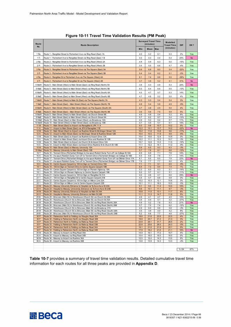
Palmerston North Area Traffic Model - Model Development and Validation Report
Beca // 23 December 2014 // Page 66 3818357 // NZ1-9382215-56 0.56
Figure 10-11 Travel Time Validation Results (PM Peak) Surveyed Travel Time
(minutes)
Min Mean Max
1 Ra Route 1 - Rangitikei Street to Fitzherbert Ave via Ring Road (East) 1A 4.0 5.2 6.1 5.3 2% Yes
1 Fi Route 1 - Fitzherbert Ave to Rangitikei Street via Ring Road (East) 1 B 4.0 4.3 4.4 5.4 25% No
2 Ra Route 2 - Rangitikei Street to Fitzherbert Ave via Ring Road (West) 2A 4.9 5.9 6.3 5.0 -15% Yes
2 Fi Route 2 - Fitzherbert Ave to Rangitikei Street via Ring Road (West) 2B 3.4 5.0 6.6 4.7 -6% Yes
3 Ra Route 3 - Rangitikei Street to Fitzherbert Ave via The Square (East) 3A 5.6 6.9 8.0 5.4 -22% Yes
3 Fi Route 3 - Fitzherbert Ave to Rangitikei Street via The Square (East) 3B 5.4 5.4 6.2 5.1 -5% Yes
4 Ra Route 4 - Rangitikei St to Fitzherbert Ave via The Square (West) 4A 6.1 7.4 8.6 5.5 -26% Yes
4 Fi Route 4 - Fitzherbert Ave to Rangitikei St via The Square (West) 4B 3.7 3.9 5.2 5.1 31% No
5 MaW Route 5 - Main Street (West) to Main Street (East) via Ring Road (North) 5A 3.8 4.3 4.8 5.3 24% No
5 MaE Route 5 - Main Street (East) to Main Street (West) via Ring Road (North) 5B 6.0 6.4 6.6 5.5 -13% Yes
6 MaW Route 6 - Main Street (West) to Main Street (East) via Ring Road (South) 6A 4.5 4.7 5.7 5.3 14% Yes
6 MaE Route 6 - Main Street (East) to Main Street (West) via Ring Road (South) 6B 4.7 4.8 5.2 5.0 4% Yes
7 MaW Route 7 - Main Street (West) to Main St (East) via The Square (North) 7A 4.3 5.3 5.4 5.4 3% Yes
7 MaE Route 7 - Main Street (East) - Main Street (West) via The Square (North) 7B 4.8 5.4 5.8 4.9 -9% Yes
8 MaW Route 8 - Main Street (West) to Main Street (East) via The Square (South) 8A 4.7 4.8 4.9 5.0 4% Yes
8 MaE Route 8 - Main Street (East) - Main Street (West) via The Square (North) 8B 3.6 5.6 7.5 5.9 5% Yes9 MaW Route 9 - Main Street (West) to Main Street (East) via Church Street 9B 4.9 4.9 5.4 5.3 8% Yes9 MaE Route 9 - Main Street (East) to Main Street (West) via Church Street 9A 5.7 6.2 8.7 5.4 -13% Yes
10 MaE Route 10 - Main Street (East) to Main Street (West) via Broadw ay 10A 4.9 5.2 5.4 5.7 11% Yes10 MaW Route 10 - Main Street (West) to Main Street (East) via Broadw ay 10B 4.7 5.5 5.7 6.1 10% Yes
11 M Route 11 - Main Street (East) to Airport via Ranagtikei & JFK 11 A 9.3 9.8 10.7 10.2 5% Yes11 A Route 11 - Airport to Main Street (East) via JFK & Ranagtikei 11B 12.2 13.1 13.7 10.2 -22% No12 M Route 12 - Main Street (East) to Airport via Ruahine Street & McGregor Street 12A 10.2 11.6 13.8 9.6 -17% Yes12 A Route 12 - Airport to Main Street (East) via McGregor Street & Ruahine Street 12B 10.4 10.5 11.9 9.9 -6% Yes13 M Route 13 - Main Street (East) to Airport via Ruahine & Airport Drive 13A 10.4 10.6 12.4 10.9 3% Yes13 A Route 13 - Airport to Main Street (East) via Airport Drive and Ruahine St 13B 10.2 11.1 12.3 10.7 -3% Yes14 M Route 14 - Main Street (East) to Airport via Church St & Airport Drive 14A 10.7 12.8 13.3 11.5 -10% Yes14 A Route 14 - Airport to Main Street (East) via Airport Drive Ruahine St & Church St 14B 11.1 12.2 14.1 11.2 -8% Yes15 M Route 15 - Main Street (East) to Massey University 15A 5.8 6.5 8.3 6.3 -3% Yes
15 Mas Route 15 - Massey University to Main Street (East) 15B 5.7 7.6 8.1 6.6 -13% Yes16 T Route 16 - Tennent Drive (Fitzherbert Bridge) to Aw apuni Rubish Dump Turn-off via College St 16A 6.9 6.9 7.1 7.8 14% Yes16 A Route 16 - Aw apuni Rubbish Dump Turn-off to Tennent Drive (Fitzherbert Bridge) via College St 16B 6.5 6.8 7.8 7.7 14% Yes17 T Route 17 - Tennent Drive (Fitzherbert Bridge) to Aw apuni Rubbish Dump Turn-off via Dittmer Drive 17A 6.1 6.5 6.5 7.9 22% No17 A Route 17 - Aw apuni Rubbish Dump Turn-off to Tennent Drive (Fitzherbert Bridge) via Dittmer Drive 17B 7.6 7.7 7.7 8.0 4% Yes18 C Route 18 - Centre Square Carpark to 100 km Sign on Tennent Drive 18A 7.1 7.1 9.1 6.5 -9% Yes18 1 Route 18 - 100 km Sign on Tennent Drive to Centre Square Carpark 18B 6.4 7.3 8.4 7.4 1% Yes19 C Route 19 - Centre Square Carpark to 100 km Sign on Pioneer Highw ay 19A 5.3 6.0 6.3 5.1 -14% Yes19 1 Route 19 - 100 km Sign on Pioneer Highw ay to Centre Square Carpark 19B 5.0 5.7 6.1 5.1 -11% Yes21 C Route 21 - Centre Square Carpark to 100 km Sign on Rangitikei St 21A 4.0 4.6 4.7 6.0 29% No21 1 Route 21 - 100 km Sign on Rangitikei St to Centre Square Carpark 21B 4.4 5.7 6.8 5.9 3% Yes22 C Route 22 - Centre Square Carpark to 100 km Sign on Milson Line 22A 10.2 10.3 12.1 10.6 3% Yes22 1 Route 22 - 100 km Sign on Milson Line to Centre Square Carpark 22B 10.1 11.1 18.3 10.5 -5% Yes23 M Route 23 - Massey University Entrance to Hospital via Te Aw e Aw e St 23A 9.1 9.5 11.4 10.5 10% Yes23 H Route 23 - Hospital to Massey Unniversity Entrance via Te Aw e Aw e St 23B 9.6 10.1 11.1 9.7 -3% Yes24 M Route 24 - Massey University Entrance to Hospital via Main St 24A 10.8 11.0 13.1 11.7 6% Yes24 H Route 24 - Hospital to Massey University Entrance via Main St 24B 11.1 11.3 14.7 11.8 5% Yes25 B Route 25 - Briscoes (Main St) to Warehouse (Church St) via Church St 25B 4.6 4.1 4.7 4.5 10% Yes25 W Route 25 - Warehouse (Church St) to Briscoes (Main St) via Church St 25A 3.4 4.4 5.1 3.2 -27% Yes26 W Route 26 - Warehouse (Church St) to Briscoes (Main St) via Ring Road (North) 26A 4.9 5.2 7.8 6.3 21% No26 B Route 26 - Briscoes (Main St) to Warehouse (Church St) via Ring Road (North) 26B 5.7 7.0 7.4 6.2 -12% Yes27 W Route 27 - Warehouse (Church St) to Briscoes (Main St) via Broadw ay 27A 4.9 6.0 6.6 5.8 -3% Yes28 W Route 28 - Warehouse (Church St) to Briscoes (Main St) via Ring Road (South) 28A 3.5 3.9 4.0 4.2 9% Yes28 B Route 28 - Briscoes (Main St) to Warehouse (Church St) via Ring Road (South) 28B 5.2 6.6 7.7 4.8 -27% Yes30 P Route 30 - Palmerston North to Feilding via Waughs Road 30A 18.6 21.6 22.6 22.5 4% Yes30 F Route 30 - Feilding to Palmerston North via Waughs Road 30B 19.8 20.7 21.2 21.3 3% Yes33 P Route 33 - Palmerston North to Feilding via Railw ay Road 33A 23.8 26.1 31.7 26.5 2% Yes33 F Route 33 - Feilding to Palmerston North via Railw ay Road 33B 22.8 25.6 29.3 24.3 -5% Yes34 P Route 34 - Palmerston North to Feilding via Railw ay Road 34A 19.1 21.0 21.9 22.1 5% Yes34 F Route 34 - Feilding to Palmerston North via Railw ay Road 34B 17.9 18.2 21.6 21.1 16% No35 M Route 35 - Massey to Airport via Ring Road 35A 14.9 16.1 17.2 16.7 4% Yes35 A Route 35 - Airport to Massey via Ring Road 35B 15.4 16.0 16.5 16.0 0% Yes36 M Route 36 - Massey to Airport via Ruahine 36A 12.5 12.4 14.3 13.5 9% Yes36 A Route 36 - Airport to Massey via Ruahine 36B 13.8 13.9 14.3 13.3 -4% Yes
% OK 87%
OK ?DiffModelled
Travel Time (minutes)
Route No.
Route Description
Table 10-7 provides a summary of travel time validation results. Detailed cumulative travel time information for each routes for all three peaks are provided in Appendix D.
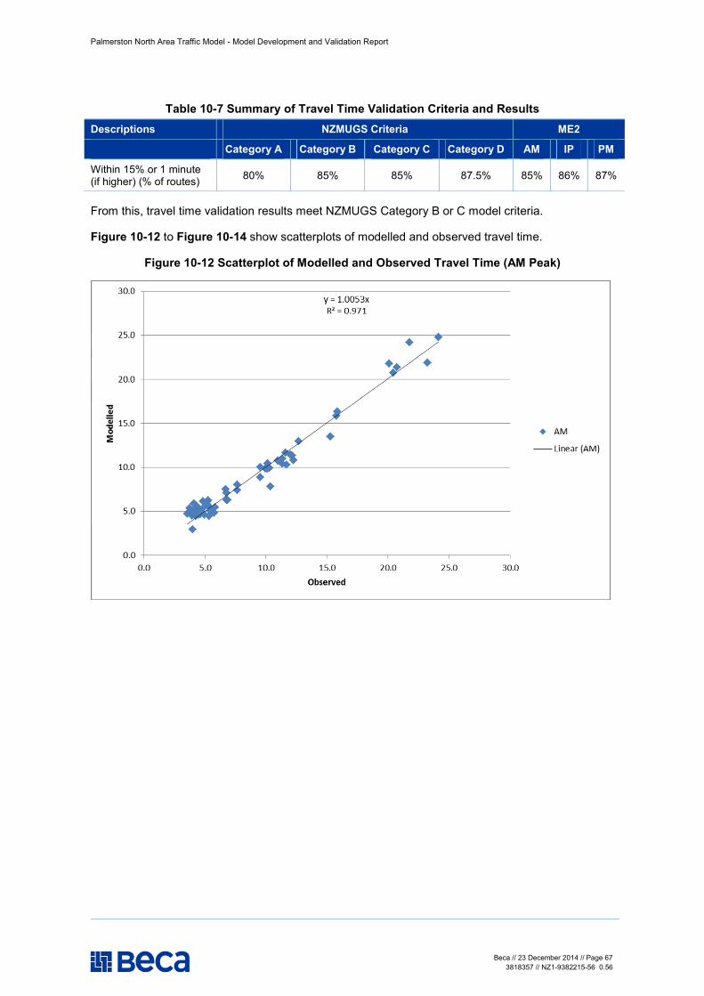
Palmerston North Area Traffic Model - Model Development and Validation Report
Beca // 23 December 2014 // Page 67 3818357 // NZ1-9382215-56 0.56
Table 10-7 Summary of Travel Time Validation Criteria and Results Descriptions NZMUGS Criteria ME2
Category A Category B Category C Category D AM IP PM
Within 15% or 1 minute (if higher) (% of routes) 80% 85% 85% 87.5% 85% 86% 87%
From this, travel time validation results meet NZMUGS Category B or C model criteria.
Figure 10-12 to Figure 10-14 show scatterplots of modelled and observed travel time.
Figure 10-12 Scatterplot of Modelled and Observed Travel Time (AM Peak)
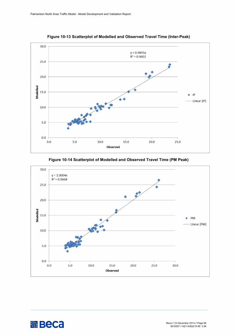
Palmerston North Area Traffic Model - Model Development and Validation Report
Beca // 23 December 2014 // Page 68 3818357 // NZ1-9382215-56 0.56
Figure 10-13 Scatterplot of Modelled and Observed Travel Time (Inter-Peak)
Figure 10-14 Scatterplot of Modelled and Observed Travel Time (PM Peak)
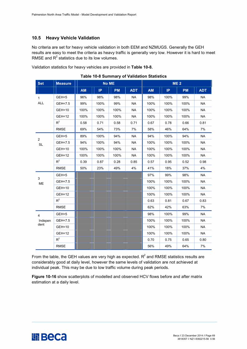
Palmerston North Area Traffic Model - Model Development and Validation Report
Beca // 23 December 2014 // Page 69 3818357 // NZ1-9382215-56 0.56
10.5 Heavy Vehicle Validation
No criteria are set for heavy vehicle validation in both EEM and NZMUGS. Generally the GEH results are easy to meet the criteria as heavy traffic is generally very low. However it is hard to meet RMSE and R2 statistics due to its low volumes.
Validation statistics for heavy vehicles are provided in Table 10-8.
Table 10-8 Summary of Validation Statistics Set Measure No ME ME 2
AM IP PM ADT AM IP PM ADT
1 ALL
GEH<5 96% 98% 98% NA 98% 100% 99% NA
GEH<7.5 99% 100% 99% NA 100% 100% 100% NA
GEH<10 100% 100% 100% NA 100% 100% 100% NA
GEH<12 100% 100% 100% NA 100% 100% 100% NA
R2 0.58 0.71 0.58 0.71 0.67 0.78 0.66 0.81
RMSE 69% 54% 73% 7% 58% 46% 64% 7%
2 SL
GEH<5 89% 100% 94% NA 94% 100% 94% NA
GEH<7.5 94% 100% 94% NA 100% 100% 100% NA
GEH<10 100% 100% 100% NA 100% 100% 100% NA
GEH<12 100% 100% 100% NA 100% 100% 100% NA
R2 0.39 0.87 0.28 0.85 0.57 0.95 0.52 0.98
RMSE 50% 23% 49% 4% 41% 18% 37% 4%
3 ME
GEH<5 97% 99% 98% NA
GEH<7.5 100% 100% 100% NA
GEH<10 100% 100% 100% NA
GEH<12 100% 100% 100% NA
R2 0.63 0.81 0.67 0.83
RMSE 62% 42% 63% 7%
4 Independent
GEH<5 98% 100% 99% NA
GEH<7.5 100% 100% 100% NA
GEH<10 100% 100% 100% NA
GEH<12 100% 100% 100% NA
R2 0.70 0.75 0.65 0.80
RMSE 56% 49% 64% 7%
From the table, the GEH values are very high as expected. R2 and RMSE statistics results are considerably good at daily level, however the same levels of validation are not achieved at individual peak. This may be due to low traffic volume during peak periods.
Figure 10-16 show scatterplots of modelled and observed HCV flows before and after matrix estimation at a daily level.
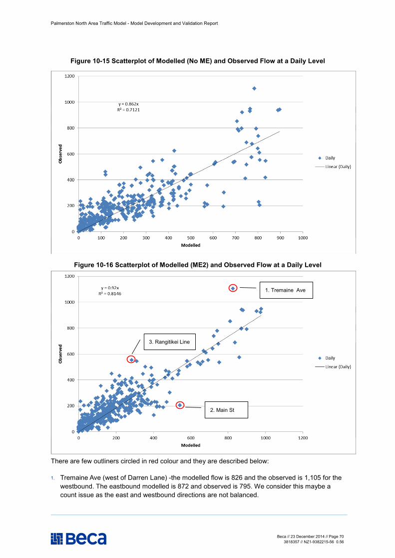
Palmerston North Area Traffic Model - Model Development and Validation Report
Beca // 23 December 2014 // Page 70 3818357 // NZ1-9382215-56 0.56
Figure 10-15 Scatterplot of Modelled (No ME) and Observed Flow at a Daily Level
Figure 10-16 Scatterplot of Modelled (ME2) and Observed Flow at a Daily Level
There are few outliners circled in red colour and they are described below:
1. Tremaine Ave (west of Darren Lane) -the modelled flow is 826 and the observed is 1,105 for the westbound. The eastbound modelled is 872 and observed is 795. We consider this maybe a count issue as the east and westbound directions are not balanced.
1. Tremaine Ave
2. Main St
3. Rangitikei Line
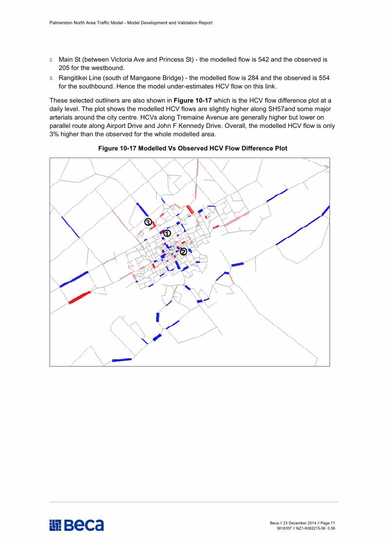
Palmerston North Area Traffic Model - Model Development and Validation Report
Beca // 23 December 2014 // Page 71 3818357 // NZ1-9382215-56 0.56
2. Main St (between Victoria Ave and Princess St) - the modelled flow is 542 and the observed is 205 for the westbound.
3. Rangitikei Line (south of Mangaone Bridge) - the modelled flow is 284 and the observed is 554 for the southbound. Hence the model under-estimates HCV flow on this link.
These selected outliners are also shown in Figure 10-17 which is the HCV flow difference plot at a daily level. The plot shows the modelled HCV flows are slightly higher along SH57and some major arterials around the city centre. HCVs along Tremaine Avenue are generally higher but lower on parallel route along Airport Drive and John F Kennedy Drive. Overall, the modelled HCV flow is only 3% higher than the observed for the whole modelled area.
Figure 10-17 Modelled Vs Observed HCV Flow Difference Plot
1
2
3

Palmerston North Area Traffic Model - Model Development and Validation Report
Beca // 23 December 2014 // Page 72 3818357 // NZ1-9382215-56 0.56
10.6 Convergence
The convergence of the model assignment iterations was measured by different criteria but convergence is mainly achieved by relative gap. Relative gap is widely used as a convergence criterion in most of the modelling software packages.
The relative gaps for the base year assignment are shown in Table 10-9.
Table 10-9 Convergence Statistics of Assignment Iterations
Converged by AM IP PM
Relative Gap 0.198% 0.193% 0.154%
Relative gap is the difference between the total travel time on the network and the total travel time on the shortest paths for the current iteration, divided by the total travel time on the network. This measures the proximity of current iteration travel time to ideal shortest route time (equilibrium).
Currently the models run approximately 15 iterations which is less than the maximum number of iterations, 40. For a relatively small project where the model stability is critical, the relative gap can be increased to 0.01% (0.0001). However tightening the convergence criteria will increase the model run time.
11 Conclusions
This report sets out the inputs and process used to develop the Palmerston North Area Traffic Model. It also sets out the results of the validation process. In general, the model validates well, with very limited Matrix Estimation required. This provides confidence that the model accurately reflects current traffic patterns in Palmerston North and forms a sound basis for forecasting.
The next (and final) stage in this project is to undertake network and land use forecasting using the model. The stage will consist of engagement with Council officers to identify committed and potential changes that can be incorporated into future year versions of the model.